A Study of Exclusive Charmless Semileptonic $B$ Decays and
Extraction of $|V_{ub}|$ at CLEO

Abstract

We have studied semileptonic $B$ decay to the exclusive charmless states $\pi$, $\rho/\omega$, $\eta$ and $\eta^{\prime}$ using the full 15.5 fb^-1 CLEO $\Upsilon(4S)$ sample, with measurements performed in subregions of phase space to minimize dependence on a priori knowledge of the form factors involved. We find total branching fractions ${\cal B}(B^{0}\to\pi^{-}\ell^{+}\nu)=(1.37\pm 0.15_{\text{stat}}\pm 0.11_{\text{sys}})\times 10^{-4}$ and ${\cal B}(B^{0}\to\rho^{-}\ell^{+}\nu)=(2.93\pm 0.37_{\text{stat}}\pm 0.37_{\text{sys}})\times 10^{-4}.$ We find evidence for $B^{+}\to\eta^{\prime}\ell^{+}\nu$, with ${\cal B}(B^{+}\to\eta^{\prime}\ell^{+}\nu)=(2.66\pm\pm 0.80_{\text{stat}}\pm 0.56_{\text{sys}})\times 10^{-4}$ and $1.20\times 10^{-4}<{\cal B}(B^{+}\to\eta^{\prime}\ell^{+}\nu)<4.46\times 10^{-4}$ (90% CL). We also limit ${\cal B}(B^{+}\to\eta\ell^{+}\nu)<1.01\times 10^{-4}$ (90% CL). By combining our $B\to\pi\ell\nu$ information with unquenched lattice calculations, we find $|V_{ub}|=(3.6\pm 0.4_{\text{stat}}\pm 0.2_{\text{sys}}{}^{+0.6}_{-0.4\text{thy}})\times 10^{-3}$.

I Introduction

$V_{ub}$ remains one of the most poorly constrained parameters of the Cabibbo-Kobayashi-Maskawa (CKM) matrix bb:CKM . Its magnitude, $|V_{ub}|$, plays a central role in testing the consistency of the CKM matrix in $B$ and $K$ meson decay processes. Inconsistency would signal existence of new classes of fundamental particles or forces. A precise determination of $|V_{ub}|$ has been the subject of considerable theoretical and experimental effort for well over a decade, and remains one of the highest priorities of flavor physics.

Measurements of exclusive charmless semileptonic decays $B\to X_{u}\ell\nu$ bb:cleoprl77y1996 ; bb:lange_cleo_exclusive ; bb:Athar:2003yg ; bb:BABARy2005 ; bb:BABARy2006 ; bb:BABARy2007 ; bb:BELLEy2007 provide a route to the determination of $|V_{ub}|$ with experimental and theoretical uncertainties complementary to the current inclusive techniques bb:PDG_vub_minireview . The primary challenge facing all measurements of semileptonic $b\to u\ell\nu$ decay is separation of the signal from the much larger $b\to c\ell\nu$ background. Exclusive $b\to u\ell\nu$ decays provide unique kinematic constraints for this purpose, particularly if a reliable estimate of the neutrino four-momentum is obtained.

In addition to the experimental challenges facing the exclusive measurements, extraction of $|V_{ub}|$ requires knowledge of the form factors that govern the dynamics of these decays. The form factors contribute both to the variation of rate, or shape, over phase space and to the overall rate via the form factor normalization. The form factors are inherently nonperturbative QCD quantities and considerable effort has been devoted to their calculation. A major recent theoretical advance has come in the form of predictions from unquenched lattice QCD (LQCD) calculations  HPQCD_2006 , which provide predictions with uncertainties claimed to be at the 10% level for $B\to\pi\ell\nu$. Light Cone Sum Rules (LCSR) techniques also provide predictions for the $B\to\pi\ell\nu$  ball_2005 and $B\to\rho\ell\nu$ form factors ball04 .

For the extraction of $|V_{ub}|$, we consider semileptonic decays to the pseudoscalar final states $\pi^{-}\ell^{+}\nu$ and $\pi^{0}\ell^{+}\nu$, for which we have the unquenched lattice QCD predictions. We also investigate the decays to vector final states $\rho^{-}\ell^{+}\nu$, $\rho^{0}\ell^{+}\nu$, and $\omega\ell^{+}\nu$. An accurate determination of the decay rate to vector final states is necessary for quantifying cross feed into the $B\to\pi\ell\nu$ rate that is ultimately used to extract $|V_{ub}|$.

In addition, we search for $B^{+}\to\eta\ell^{+}\nu$ and $B^{+}\to\eta^{\prime}\ell^{+}\nu$. Because semileptonic decays involve only a single hadronic current, they additionally offer a probe of the QCD phenomena underlying fully hadronic decay. In particular, the $B\to\eta\ell^{+}\nu$ and $B\to\eta^{\prime}\ell^{+}\nu$ decays probe the singlet or QCD anomaly component of the $\eta^{\prime}$ meson etap:FKS . This component may be responsible for the unexpectedly high branching fractions observed in $B\to\eta^{\prime}X_{s}$ decays etap:cleo:etapxs ; etap:babar:etapxs ; etap:belle:etapxs . A measurement of $\mathcal{B}(B^{+}\to\eta\ell^{+}\nu)$ was included in previous CLEO studies bb:Athar:2003yg , and in 2006, BaBar released preliminary upper limits for both $B\to\eta\ell\nu$ and $B\to\eta^{\prime}\ell\nu$ branching fractions BaBar_eta_ichep06 .

This paper describes the CLEO studies of these seven exclusive $b\to u\ell\nu$ decay modes. The excellent hermeticity of the CLEO detector and the symmetric $e^{+}e^{-}$ beam configuration of the Cornell Electron Storage Ring (CESR) allows for precise determination of the neutrino four-momentum. In contrast to asymmetric $B$ factories, the lack of a center of mass boost along the beam direction enhances the fraction of $\Upsilon(4S)\to B\bar{B}$ events in which all particles are contained in the detector fiducial region. This allows more stringent selection criteria to be placed on the reconstructed neutrino that improve neutrino resolution without degrading efficiency. This ultimately results in a cleaner separation between signal and background that enables measurements of exclusive semileptonic rates at CLEO to be competitive with higher statistics analyses carried out at asymmetric $B$ factories.

We study all seven decay modes simultaneously, extracting independent measurements in subregions of phase space in order to minimize a priori dependence on form factor shape predictions. While the general method is similar to the previous CLEO study bb:Athar:2003yg , the current analysis further reduces the sensitivity to the decay form factors by decreasing the lower bound on the charged-lepton momentum requirement for the vector modes from $1.5$ GeV/$c$ to $1.0$ (1.2) GeV/$c$ for electrons (muons) and, in addition, measuring partial rates for vector modes in bins of lepton decay angle. Furthermore, our measurements of the rates over the $\rho\ell\nu$ phase space allow us to test the validity of form factor shape calculations in that mode.

To increase signal efficiency, we have also modified the phase-space binning in the region of high meson recoil momentum, where continuum $e^{+}e^{-}\to q\bar{q}$ backgrounds contribute.

This analysis utilizes a total of $15.4\times 10^{6}$ $B\overline{B}$ decays obtained at the $\Upsilon(4S)$, a relative increase of 60% from the previous CLEO analysis bb:Athar:2003yg . The results presented here supersede those of the previous analysis.

The paper is organized as follows. Sections II and III discuss the role of form factors for extraction of $|V_{ub}|$ and the relation of the QCD anomaly to the $B\to\eta\ell\nu$ and $B\to\eta^{\prime}\ell\nu$ branching fractions. Section IV describes our reconstruction technique. Section V describes our fitting method, fit components, and fit results. Section VI describes the systematic uncertainties. Section VII interprets the results. Throughout the paper, charge conjugate modes are implied. A more detailed description of the analysis technique can be found in Reference bb:mrs43_thesis .

II Exclusive Charmless Semileptonic Decays

Figure 1: Predictions for $d\Gamma(B\to\pi\ell\nu)/dq^{2}$ for a variety form factor calculation techniques HPQCD_2006 ; spd ; isgw2 ; ball_2005 illustrate the range of variation of the predicted $q^{2}$–dependence.

Figure 2: Predictions for $d\Gamma(B\to\rho\ell\nu)/dq^{2}$ (left) and $d\Gamma(B\to\rho\ell\nu)/d\cos\theta_{Wl}$ (right) for a variety of form factor calculation techniques ball04 ; meli ; isgw2 ; ukqcd98 illustrate the range of variation of the predicted $q^{2}$ and $\cos\theta_{Wl}$ dependence.

For $B\to V_{u}\ell\nu$, where $V_{u}$ is a charmless vector meson, the partial width is

$$\frac{d\Gamma}{dq^{2}\,dC_{\theta}}=\kappa kq^{2}\left[S^{2}_{\theta}H_{0}^{2}+\frac{C_{-}^{2}H_{+}^{2}+C_{+}^{2}H_{-}^{2}}{2}\right].$$ (1)

Here, $\kappa=\frac{|V_{ub}|^{2}G_{F}^{2}}{128\pi^{3}M_{B}^{2}}$, $k$ is the $V_{u}$ momentum, $q^{2}$ is the mass squared of the virtual $W$ ($W^{*}$), $C_{\theta}$ ($S_{\theta}$) is the cosine (sine) of the angle $\theta_{Wl}$ between the charged lepton in the $W^{*}$ rest frame and the $W^{*}$ in the $B$ rest frame, and $C_{\pm}=1\pm C_{\theta}$. $H_{\pm}$ and $H_{0}$ are the magnitudes of the $W$ helicity amplitudes, which can be expressed in the massless lepton limit in terms of three $q^{2}$–dependent form factors Gilman_and_Singleton , $g$, $a_{+}$, and $f$, as

$$\left|H_{\pm}\right|^{2}=\left[f\left(q^{2}\right)\mp 2M_{B}kg\left(q^{2}\right)\right]^{2}$$ (2)

(3)

$$\left|H_{0}\right|^{2}=\frac{M_{B}^{4}}{4q^{2}M_{V_{u}}^{2}}\times$$

$$\Bigg{[}\left(1-\frac{M_{V_{u}}^{2}+q^{2}}{M_{B}^{2}}\right)f(q^{2})+4k^{2}a_{+}(q^{2})\Bigg{]}.$$

For a final state pseudoscalar meson $P_{u}$, $H_{\pm}=0$, and the rate depends on a single form factor $f_{+}(q^{2})$:

$$\frac{d\Gamma\left(B\to P_{u}\ell\nu\right)}{dq^{2}}=\left|V_{ub}\right|^{2}\frac{G_{F}^{2}}{24\pi^{3}}k^{3}\left|f_{+}\left(q^{2}\right)\right|^{2}.$$ (4)

The structure of the differential decay rates allows us to draw some general conclusions regarding the properties of the semileptonic decay modes studied here. For the $\rho(\omega)\ell\nu$ transitions, the left-handed, $V-A$, nature of the charged current at the quark level manifests itself at the hadronic level as $|H_{-}|>|H_{+}|$. The $H_{-}$ contribution is also expected to dominate the $H_{0}$ contribution, leading to a forward-peaked distribution for $\cos\theta_{Wl}$. The pseudoscalar modes exhibit a $\sin^{2}\theta_{Wl}$ dependence, independent of the form factor since the rate is independent of $\theta_{Wl}$. They also depend on an extra factor of $p_{X_{u}}^{2}$, which suppresses the rate near $q^{2}_{\text{max}}$ ($p_{X_{u}}=0$). Taken together, these two effects give the pseudoscalar modes a softer charged lepton momentum spectrum than the vector modes.

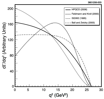
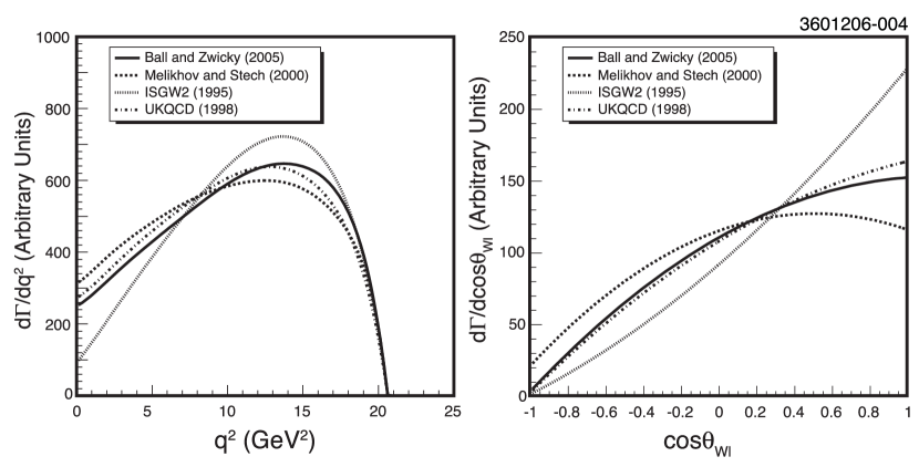
Recent results for $f_{+}(q^{2})$ from lattice calculations with dynamical quarks HPQCD_2006 provide a marked theoretical advance in form factor calculations. However, significant theoretical uncertainties still remain in the $q^{2}$ dependence of the form factors, particularly in the non-$\pi\ell\nu$ decay modes. Figures 1 and 2 illustrate the variation of form factor predictions for a variety of theoretical techniques. The effect of these uncertainties on the total rate measurements can be mitigated by measuring partial rates in several regions of phase space.

In the $\pi\ell\nu$ modes the rates extracted in our chosen $q^{2}$ intervals will be largely independent of the assumed form factor shapes. In the vector modes, however, the three form factors interfere and uncertainties in this interference, particularly for $\cos\theta_{Wl}<0$, lead to a form factor systematic uncertainty. To reduce this uncertainty, we have included the $\cos\theta_{Wl}<0$ data in the fit, rather than relying on our assumed form factors to extrapolate into this region. There is substantial cross feed from the $\cos\theta_{Wl}<0$ region of $B\to\rho\ell\nu$ phase space into the reconstructed $B\to\pi\ell\nu$ decays. As a result, the the largest form factor systematic uncertainty in the previous CLEO $B\to\pi\ell\nu$ measurement arose from the $B\to\rho\ell\nu$ mode. Our improved measurements over a larger region of phase space better constrain the $B\to\rho\ell\nu$ rate and reduce this systematic uncertainty by roughly an order of magnitude.

III QCD Anomaly in $B\to\eta^{(\prime)}\ell\nu$

As mentioned in the introduction, we can check for consistency and probe for new information in quark symmetries by measuring the $B\to\eta\ell\nu$ and $B\to\eta^{\prime}\ell\nu$ branching fractions. Branching fraction measurements for $B\to\eta^{\prime}X_{s}$ cleo_etapk_1997 ; etap:cleo:etapxs ; etap:babar:etapxs ; etap:belle:etapxs yield larger than expected results, indicating extra couplings in the $B\to\eta^{\prime}$ form factor. Measurements at CLEO of $\eta^{\prime}$ production in $\Upsilon(1S)$ decays Artuso:2002px limit the contribution of the $\eta^{\prime}\to g^{*}g$ form factor to the anomalously high $B\to\eta^{\prime}X_{s}$ rate. This unexpected rate may be accounted for by the additional QCD Anomaly QCDAnomalyDefinition contribution to the $\eta^{\prime}$ axial vector current, which can be cleanly measured in semileptonic decays etap:CSK . The QCD Anomaly provides additional gluon couplings to singlet states, but no additional couplings to non-singlet states.

The $SU(3)$ octet of the u, d, and s quarks contain the $\pi^{-}$, $\pi^{+}$, $K^{0}$, $K^{-}$, $K^{+}$ mesons as well as sums of the $\pi^{0}$ with the octet triplet $\eta^{8}\equiv\frac{1}{\sqrt{6}}(\bar{u}u+\bar{d}d-2\bar{s}s)$. The singlet of this symmetry is $\eta^{0}\equiv\frac{1}{\sqrt{3}}(\bar{u}u+\bar{d}d+\bar{s}s)$. The physical $\eta$ and $\eta^{\prime}$ mesons appear to be primarily made up of combinations of the $\eta^{0}$ singlet state and the $\eta^{8}$ triplet state. Since the $\eta$ mass is so much closer to the $K$ masses, it is primarily $\eta^{8}$. The $\eta^{\prime}$ is mostly the $\eta^{0}$ singlet, which possesses the strong gluon couplings in the axial vector current. A measurement of the ratio of $\mathcal{B}(B\to\eta^{\prime}\ell\nu)$ to $\mathcal{B}(B\to\eta\ell\nu)$ provides experimental input needed to extract the strength of these gluon couplings.

Once the sizes of these couplings have been determined for a particular model using the semileptonic $B\to\eta\ell\nu$ and $B\to\eta^{\prime}\ell\nu$ decays, the same form factor parameterization can be used to check for consistency with the $B\to\eta^{\prime}X_{s}$ decays (see section VII.3.)

IV Event Reconstruction and Selection

This study utilizes the full 15.5 fb^-1 set of data collected at the $\Upsilon(4S)$ with the CLEO II Kubota:1991ww , CLEO II.5 Hill:1998ea and CLEO III Peterson:2002sk detectors at CESR. The analysis rests upon associating the missing energy and momentum in each event with the neutrino four-momentum, an approach enabled by the excellent hermeticity and resolution of the CLEO detectors. Charged particles are detected over at least 93% of the total solid angle for all three detector configurations, and are measured in a solenoidal magnetic field with a momentum resolution of 0.6% at 2 GeV/$c$. Photons and electrons are detected in a CsI(Tl) electromagnetic calorimeter that covers 98% of the $4\pi$ solid angle. A typical $\pi^{0}$ mass resolution is 6 MeV$/c^{2}$. Unless otherwise noted, all kinematic quantities are measured in the laboratory frame.

Electrons satisfying $p>200\text{ MeV}/c$ are identified over 90% of the solid angle by using the ratio of energy deposited in the calorimeter to track momentum in conjunction with specific ionization ($dE/dx$) information from the main drift chamber, shower shape information, and the difference between extrapolated track position and the cluster centroid. Depending on detector configuration, either time-of-flight (CLEO II/II.5) or Ring Imaging Čerenkov Artuso:2005dc (CLEO III) measurements provide additional $e^{\pm}/K^{\pm}$ separation.

Particles in the polar angle range $|\cos\theta|<0.85~{}(0.65)$ that register hits in counters beyond five interaction lengths are accepted as signal muons with the CLEO II/II.5 (CLEO III) detector configurations. Those with $|\cos\theta|<0.71$ and hits between three and five interaction lengths are used in a multiple-lepton veto, discussed below.

We restrict signal electron and muon candidates to the momentum interval $1.0<p<2.8\text{ GeV}/c$ and $1.2<p<2.8\text{ GeV}/c$, respectively. The lower limits are determined by excessive background contributions for electrons, and by identification efficiency for muons. We also require that the lepton candidate tracks have signals from at least 40% of their potential drift chamber layers and are consistent with originating from the beam spot.

Momentum-dependent lepton identification efficiencies and the rates for hadrons being misidentified as a lepton (“fake rates”) for both electrons and muons are measured in data by examining the rate at which the decay products from cleanly identified $\Lambda\to p\pi^{-}$, $K^{0}_{S}\to\pi^{+}\pi^{-}$, and $D^{*+}\to\pi^{+}D^{0}\to\pi^{+}K^{-}\pi^{+}$ decays satisfy lepton identification criteria. Within the signal electron fiducial and momentum regions, the identification efficiency exceeds 90% while the fake rate is about $0.1\%$. For signal muons above 1.5 GeV$/c$, the identification efficiency also averages above 90%. For muons below 1.5 GeV$/c$, the five interaction length requirement causes the efficiency to fall rapidly to about 30% at the lowest momentum of 1.2 GeV$/c$. The muon fake rate is about 1%. The measured efficiencies and fake rates are employed in all Monte Carlo (MC) simulations.

Each charged track that is not identified as an electron or muon is assigned the most probable of the pion, kaon or proton mass hypotheses. The probability for each mass hypothesis is formed from an identification likelihood, based upon the specific ionization measurements in the drift chamber and either the time-of-flight or Čerenkov photon angle measurements, and the relative production fractions for pions, kaons and protons at that momentum in generic $B$ meson decay.

To reconstruct the undetected neutrino we associate the neutrino four-momentum $p_{\nu}$ with the missing four-momentum $p_{\mathrm{miss}}$. In the process $e^{+}e^{-}\to\Upsilon(4S)\to B\bar{B}$, the total energy of the beams is imparted to the $B\bar{B}$ system; at CESR that system is very nearly at rest because beam energies are symmetric and the beam crossing angle is small ($\approx$ 2 mrad). The missing four-momentum in an event is given by $p_{\mathrm{miss}}=(E_{\mathrm{miss}},\vec{p}_{\mathrm{miss}})=p_{\mathrm{total}}-\sum p_{\mathrm{charged}}-\sum p_{\mathrm{neutral}}$, where the event four-momentum $p_{\mathrm{total}}$ is known from the energy and crossing angle of the CESR beams and $p_{\mathrm{charged}}$ and $p_{\mathrm{neutral}}$ are the four-momenta of charged and neutral particles explicitly reconstructed by the detector. Charged and neutral particles pass selection criteria designed to achieve the best possible $|\vec{p}_{\mathrm{miss}}|$ resolution by balancing the efficiency for detecting true particles against the rejection of false ones.

For the charged four-momentum sum $\sum p_{\mathrm{charged}}$, optimal selection is achieved with topological criteria that minimize multiple-counting resulting from low-momentum tracks that curl in the magnetic field, charged particles that decay in flight or interact within the detector, and spurious tracks. Tracks that are actually segments of a single low transverse momentum “curling” particle can be mis-reconstructed as two (or more) separate outgoing tracks with opposite charge and roughly equal momentum. These tracks are identified by selecting oppositely charged track pairs whose innermost and outermost diametric radii each match within 14 cm and whose separation in $\phi$ is within 180${}^{\circ}\pm 20^{\circ}$. We choose the track segment that will best represent the original charged particle based on track quality and distance of closest approach information. We employ similar algorithms to identify particles that curl more than once, creating three or more track segments. We also identify tracks that have scattered or decayed in the drift chamber, causing the original track to end and one or more tracks to begin in a new direction. We keep only the track segment with the majority of its hits before the interaction point. Spurious tracks are identified by their low hit density and/or low number of overall hits, and rejected.

For the neutral four-momentum sum, $\sum p_{\mathrm{neutral}}$, clusters resulting from the interactions of charged hadrons must be avoided. As a first step, calorimeter showers passing the standard CLEO proximity-matching (within 15 cm of a charged track) are eliminated. Optimization studies also revealed that all showers under 50 MeV should be eliminated. The processes that result in separately reconstructed showers (“splitoffs”) within about 25^∘ of a proximity-matched shower tend to result in an energy distribution over the $3\times 3$ central array of the splitoff shower that “points back” to the core hadronic shower. We combine this pointing information with the ratio of energies in the $3\times 3$ to $5\times 5$ arrays of crystals, whether the shower forms a good $\pi^{0}$, and the MC predictions for relative energy spectra for true photons versus splitoff showers to provide an optimal suppression of the splitoff contribution.

Signal MC events show a $|\vec{p}_{\text{miss}}|$ resolution of $\approx 0.1$ GeV/$c$ and an $E_{\text{miss}}$ resolution of $\approx 0.2$ GeV after all analysis cuts.

To further enhance the association of the missing momentum with an undetected neutrino in our final event sample, we require that the missing mass, $M^{2}_{\text{miss}}\equiv E^{2}_{\text{miss}}-|\vec{p}_{\text{miss}}|^{2}$, be consistent within resolution with a massless neutrino. Specifically, since the $M^{2}_{\text{miss}}$ resolution scales as $\sim 2E_{\text{miss}}/\sigma_{E_{\text{miss}}}$, for each exclusive $B\to X_{u}\ell\nu$ mode we reconstruct, we require $M^{2}_{\text{miss}}/2E_{\text{miss}}$, with typical ranges of $-0.5<M^{2}_{\text{miss}}/2E_{\text{miss}}<0.3\ \text{GeV}$. The criterion was optimized for each decay mode using independent samples of MC simluations for signal and background processes.

Association of the missing four-momentum with the neutrino four-momentum is only valid if the event contains no more than one neutrino and all true particles are detected. For events with additional missing particles or double-counted particles, the signal modes tend not to reconstruct properly, while background processes tend to smear into our sensitive regions. Hence it is worthwhile to reject events in which missing particles are likely. We exclude events containing more than one identified lepton, which indicates an increased likelihood for multiple neutrinos.

We require the angle of the missing momentum with respect to the beam axis satisfy $|\cos\theta|<0.96$. In addition to suppressing events in which particles exited the detector along the beam line, this requirement also suppresses events resulting from a collision of radiated photons from the beams. These two-photon events are background to $B\bar{B}$ events and are typically characterized by a large missing momentum along the beam axis.

A nonzero net charge $Q$ indicates at least one missed or doubly counted charged particle. The $Q=0$ sample offers the greatest purity. For the pseudoscalar modes, use of the $|Q|=1$ in addition to the $Q=0$ sample offers a statistical advantage. Events from the subset in which a very soft pion from a $D^{*}$ decay was not reconstructed in particular have only a modestly distorted missing momentum. While we retain the $|Q|=1$ sample, we treat it separately from $Q=0$ sample in reconstruction and fitting so that the statistical power of the latter sample, with its better signal to background ratio, is not diluted. For the vector modes, which have the poorest signal to background ratios, we require $Q=0$ because systematic errors associated with the normalization of the larger background in the $|Q|=1$ sample outweigh the statistical benefits.

After our selection criteria, the remaining $b\to c\ell\nu$ background events are dominated by events that contain either a $K_{L}$ meson or an additional neutrino that is roughly collinear with the signal neutrino.

With an estimate of the neutrino four-momentum in hand, we can employ full reconstruction of our signal modes. Because the resolution on $E_{\text{miss}}$ is so much larger than that for $|\vec{p}_{\text{miss}}|$, we use $(E_{\nu},\vec{p}_{\nu})=(|\vec{p}_{\text{miss}}|,\vec{p}_{\text{miss}})$ for full reconstruction. The neutrino combined with the signal charged lepton ($\ell$) and hadron ($h$) should satisfy, within resolution, the constraints on energy, $\Delta E\equiv(E_{\nu}+E_{\ell}+E_{h})-E_{\text{beam}}\approx 0$, and on momentum, $M_{h\ell\nu}\equiv[E_{\text{beam}}^{2}-|\alpha\vec{p}_{\nu}+\vec{p}_{\ell}+\vec{p}_{h}|^{2}]^{\frac{1}{2}}\approx M_{B}$, where $\alpha$, a momentum scaling factor, is chosen such that $\alpha E_{\nu}+E_{\ell}+E_{h}-E_{\text{beam}}=0$. The neutrino momentum resolution dominates the $\Delta E$ resolution, so the momentum scaling corrects for the mismeasurement of the magnitude of the neutrino momentum in the $M_{h\ell\nu}$ calculation. This correction also reduces the correlation between $M_{h\ell\nu}$ and $\Delta E$ mismeasurement. Uncertainty in the neutrino direction remains as the dominant source of smearing in this mass calculation.

We reconstruct $q^{2}=M_{W^{*}}^{2}=(p_{\nu}+p_{\ell})^{2}$ for each decay from the reconstructed charged lepton four–momentum and the missing momentum. In addition to using the scaled reconstructed momentum $\alpha\vec{p}_{\nu}$ described above, the direction of the missing momentum is changed through the smallest angle consistent with forcing $M_{h\ell\nu}=M_{B}$. This procedure results in a $q^{2}$ resolution of 0.3 GeV², independent of $q^{2}$.

A signal charged $\pi^{+}$ candidate must have the pion hypothesis as its most probable particle ID outcome, and it must not be a daughter in any reconstructed $K_{s}$ decay. A $\pi^{0}$ candidate must have a $\gamma\gamma$ mass within 2 standard deviations of the $\pi^{0}$ mass and an energy greater than $250\text{ MeV}$. Each daughter shower must have an energy greater than $30\text{ MeV}$. Combinatoric background levels outstrip efficiency gains below either of these requirements.

Reconstructed $\rho^{0}\to\pi^{+}\pi^{-}$ and $\rho^{+}\to\pi^{+}\pi^{0}$ candidates are accepted within 285 MeV$/c^{2}$ of the nominal $\rho$ mass to accommodate the broad $\rho$ resonance width. The $\pi\pi$ mass ranges are divided into three 95 MeV$/c^{2}$ intervals for the remainder of the reconstruction and fitting. We accept $\omega$ candidates, reconstructed via its $\pi^{+}\pi^{-}\pi^{0}$ decay, within 30 MeV$/c^{2}$ of the nominal $\omega$ mass, and, similar to the $\rho$ modes, the $\pi^{+}\pi^{-}\pi^{0}$ invariant mass region is divided into three equal intervals of 10 MeV$/c^{2}$. This division in both modes makes the fit sensitive to signal through rough $\rho/\omega$ line shape information. Except where noted, plots in this paper will include data from only the invariant mass interval centered on the resonance mass although data from all three regions are included in the fit.

We reconstruct $\eta$ in both the $\gamma\gamma$ and the $\pi^{+}\pi^{-}\pi^{0}$ decay modes. For $\gamma\gamma$, we require the reconstructed mass to be within 2 standard deviations (about 26 MeV$/c^{2}$) of the $\eta$ mass and each shower to have $\cos\theta<0.81$ relative to the beam pipe. Showers within a reconstructed $\pi^{0}$ are vetoed. For the $\eta\to\pi^{+}\pi^{-}\pi^{0}$ submode, the $\pi^{0}$ must be within 2 standard deviations of the $\pi^{0}$ mass and statisfy $E_{\pi^{0}}>225$ MeV. To reduce combinatoric backgrounds, the invariant mass of the two charged pion tracks must satisfy $M_{\pi\pi}<M_{\eta}-M_{\pi^{0}}+0.05$ GeV$/c^{2}$.

Figure 3: The shape of the mass of the $\rho$ in $B\to\rho\ell\nu$ and $\eta^{\prime}\to\rho\gamma$. Limited phase space in $\eta^{\prime}\to\rho\gamma$ produces the asymmetry about the nominal $\rho$ mass in this mode. Histograms are normalized to equal area.

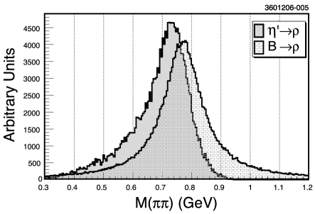
The $\eta^{\prime}$ mode is reconstructed in $\eta^{\prime}\to\rho\gamma$ and $\eta^{\prime}\to\eta\pi\pi;~{}\eta\to\gamma\gamma$. Selection criteria are optimized separately based on the event net charge and $q^{2}$ where we distinguish between $q^{2}>10~{}\text{GeV}^{2}$ and $q^{2}<10~{}\text{GeV}^{2}$. Here we specify the requirements for the $Q=0$ and $q^{2}<10~{}\text{GeV}^{2}$ sample, for which we have the greatest sensitivity. For $\eta^{\prime}\to\rho\gamma$, combinatoric backgrounds are reduced by requiring $\theta_{\pi\gamma}$, the angle between a pion and the photon in the $\rho$ rest frame, to satisfy $|\cos\theta_{\pi\gamma}|<0.925$. Photons from $\pi^{0}$ candidates were vetoed. We accept $\rho$ candidates within the mass range 0.3 to 0.9 GeV$/c^{2}$, where the range is subdivided into four roughly equal mass bins. Note that phase space restrictions in $\eta^{\prime}\to\rho\gamma$ distort the $\rho$ line shape at high $\pi\pi$ mass (Figure 3). The line shape falls rapidly to zero at $M_{\pi\pi}=0.9$ GeV$/c^{2}$, so the largest mass bin, $0.78$ GeV/$c^{2}~{}-~{}0.9$ GeV$/c^{2}$, is expected to have relatively little signal. That mass region is primarily used in the fit to constrain the background level at lower mass. The reconstructed $\eta^{\prime}$ mass must be within 2.5 standard deviations of the nominal $\eta^{\prime}$ mass.

For the $\eta^{\prime}\to\eta\pi\pi~{}(\eta\to\gamma\gamma)$ mode, the $\eta$ daughter photons must satisfy the same criteria as the $\eta$ in $\eta\ell\nu$. We also require $E_{\eta}>300$ MeV. Finally, we require the reconstructed $\eta^{\prime}$ and $\eta$ masses to satisfy $(\sigma^{2}_{\eta^{\prime}}+\sigma^{2}_{\eta})^{1/2}<3.75$, where $\sigma_{\eta(\eta^{\prime})}$ is the number of standard deviations of the reconstructed mass away from the nominal mass.

We minimize multiple candidates per event to simplify statistical interpretation. Within each $\pi$, $\eta$ or $\eta^{\prime}\to\eta\pi^{+}\pi^{-}$ mode, we allow only one candidate within the region $5.175\leq M_{h\ell\nu}<5.2875$ GeV/$c^{2}$ and $-0.75<\Delta E<0.25$ GeV used in the fit (Section V). Within a mode, multiple candidates are resolved by choosing the one with the smallest $|\Delta E|$. For the vector and the $\eta^{\prime}\to\pi^{+}\pi^{-}\gamma$ modes, the $|\Delta E|$ criterion combined with large combinatorics outside the signal region can induce a severe efficiency loss. To mitigate that loss, we select the best candidate separately within each of the individual $M_{\pi\pi}$ or $M_{3\pi}$ ranges. The $|\Delta E|$ criterion induces only very slight peaking in backgrounds, which is modeled by the MC generated distributions used to fit the data.

Figure 4: A comparison of $\left|\hat{t}_{\text{cand}}\cdot\hat{t}_{\text{ROE}}\right|$ for $B\to\pi\ell\nu$ signal MC (shaded) and off-resonance continuum data (open).

Figure 5: A comparison of $R2$ for $B\to\pi\ell\nu$ signal MC (shaded) and off-resonance continuum data (open).

Backgrounds arise from the $e^{+}e^{-}\to q\bar{q}$ and $e^{+}e^{-}\to\tau^{+}\tau^{-}$ continuum, fake leptons, $b\to c\ell\nu$, and $B\to X_{u}\ell\nu$ modes other than the signal modes. Backgrounds from continuum processes make up approximately 75% of the total cross section at the $\Upsilon(4S)$ energy. The continuum processes typically produce two collinear jets of hadrons, and the jet-like shape of the continuum events can be used to separate those events from the isotropic $B\bar{B}$ resonance events. To do this, we employ a Fisher Discriminant fishorig constructed from twelve variables that describe event shape.

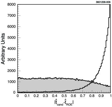
The first input variable is $\left|\hat{t}_{\text{cand}}\cdot\hat{t}_{\text{ROE}}\right|$, where $\hat{t}_{\text{cand}}$ is the thrust axis obtained using our candidate particles (excluding the neutrino), and $\hat{t}_{\text{ROE}}$ that for the remaining particles in the event. Continuum events typically have hadrons collimated into jets and therefore $\left|\hat{t}_{\text{cand}}\cdot\hat{t}_{\text{ROE}}\right|$ will peak near one (shown in Figure 4). For $\Upsilon(4S)\to B\bar{B}$, the $B$ mesons are nearly at rest and the thrust directions from the two $B$ decays will be uncorrelated; therefore $\left|\hat{t}_{\text{cand}}\cdot\hat{t}_{\text{ROE}}\right|$ will be uniformly distributed.

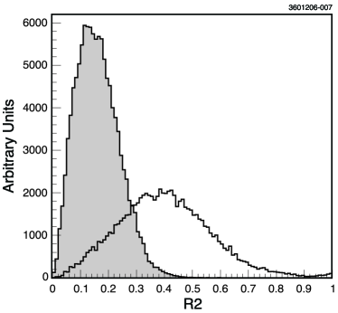
We also use the ratio of the second to zeroth Fox-Wolfram moments bb:fox_wolfram , $R2\equiv H_{2}/H_{0}$. The jet structure present in continuum events enhances the second moment and therefore the ratio $R2$ tends to one for jet-like continuum events and to zero for isotropic $B\bar{B}$ event (Figure 5).

These two variables provide the main discrimination between $B\bar{B}$ and continuum events. To gain further discriminating power we also consider the angle $\theta$ between the thrust axis of the entire event, $\hat{t}_{\text{event}}$, and the beam axis. For $B\bar{B}$ events this variable will be randomly distributed, while for continuum events the $\hat{t}_{\text{event}}$ will align with the jet axis and be distributed with approximately the $1+\cos^{2}\theta$ dependence of the cross section for $e^{+}e^{-}\to q\bar{q}$.

The remaining nine variables track the momentum flow of the event into nine forward-backward cones about the event thrust axis, each spanning 10^∘ in polar angle from the thrust axis. We optimize the continuum suppression criterion for each mode (and each subregion of phase space for each mode) separately. Due to their jet-like nature, continuum backgrounds typically reconstruct with low $q^{2}$ and can be largely isolated at $q^{2}<2$ GeV². The continuum suppression has an efficiency of roughly 15% for continuum background and 90% for signal $B\to\pi\ell\nu$ events.

The signal selection efficiencies, averaged over phase space, for the restricted signal region range from $\approx 0.5-4\%$ and are summarized in Table 1. For cases such as $\eta$ and $\eta^{\prime}$, where we only reconstruct a fraction of the decay modes, the branching fractions pdg06 to the modes we reconstruct are included in the efficiency.

Table 1: The reconstruction efficiency and fit signal yield for each final state. Both numbers are integrated over all phase space, using the nominal form factors for our fit (Section V). The efficiencies include the branching fractions for the reconstructed modes of the signal hadron. For the case of $\rho\ell\nu$ and $\omega\ell\nu$ the efficiency and yield in the central mass bin are reported. Errors on the yield are statistical only.

Decay Mode	Efficiency	Fit Yield [Events]
$B\to\pi^{\pm}\ell\nu$	4.3%	$179\pm 20$
$B\to\pi^{0}\ell\nu$	2.6%	$60\pm 6$
$B\to\eta\ell\nu$	1.0%	$14\pm 7$
$B\to\rho^{\pm}\ell\nu$	0.8%	$71\pm 9$
$B\to\rho^{0}\ell\nu$	1.6%	$79\pm 10$
$B\to\omega\ell\nu$	0.7%	$34\pm 4$
$B\to\eta^{\prime}\ell\nu$	0.5%	$41\pm 12$

V Extraction of Branching Fractions

V.1 Method and Binning

Table 2: The $q^{2}$ versus $\cos\theta_{Wl}$ intervals for which we extract partial branching fractions for each decay mode.

Mode	Index	$q^{2}$ Range [GeV2]	$\cos\theta_{Wl}$ Range
$\pi\ell\nu$	1	$0<q^{2}<2$	${}^{-}1<\cos\theta_{Wl}<1$
$\pi\ell\nu$	2	$2<q^{2}<8$	${}^{-}1<\cos\theta_{Wl}<1$
$\pi\ell\nu$	3	$8<q^{2}<16$	${}^{-}1<\cos\theta_{Wl}<1$
$\pi\ell\nu$	4	$q^{2}>16$	${}^{-}1<\cos\theta_{Wl}<1$
$\rho\ell\nu$	1	$0<q^{2}<2$	${}^{-}1<\cos\theta_{Wl}<1$
$\rho\ell\nu$	2	$2<q^{2}<8$	${}^{-}1<\cos\theta_{Wl}<1$
$\rho\ell\nu$	3	$8<q^{2}<16$	$0<\cos\theta_{Wl}<1$
$\rho\ell\nu$	4	$q^{2}>16$	$0<\cos\theta_{Wl}<1$
$\rho\ell\nu$	5	$q^{2}>8$	${}^{-}1<\cos\theta_{Wl}<0$
$\eta\ell\nu$	-	all	${}^{-}1<\cos\theta_{Wl}<1$
$\eta^{\prime}\ell\nu$	-	all	${}^{-}1<\cos\theta_{Wl}<1$

In order to determine partial branching fractions as a function of $q^{2}$ for $B\to\pi\ell\nu$, and as a function of both $q^{2}$ and $\cos\theta_{Wl}$ for $B\to\rho\ell\nu$ we divide the reconstructed candidates into the regions defined in Table 2. The variables $\Delta E$ and $M_{h\ell\nu}$ provide sensitivity to signal events and therefore in general we bin the data into seven coarse regions spanning the ranges $5.1750\leq M_{h\ell\nu}<5.2875$ GeV/$c^{2}$ and $-0.75<\Delta E<0.25$ GeV in the $\Delta E-M_{h\ell\nu}$ plane. We are primarily sensitive to signal within the range defined by $5.2650~{}\text{GeV}/c^{2}<M_{h\ell\nu}<5.2875~{}\text{GeV}/c^{2}$ and $-0.15~{}\text{GeV}<\Delta E<0.25~{}\text{GeV}$. The binning choice results from a compromise between sensitivity to the signal processes versus reliance on our simulations to reproduce in detail the signal and background shapes, which depends critically on the modeling of the missing energy and momentum.

In all of the pseudoscalar modes, we obtain $\Delta E$ versus $M_{h\ell\nu}$ distributions separately for the $|Q|=1$ and $Q=0$ subsamples. This separation allows us to take full statistical advantage of the cleaner $Q=0$, while obtaining some statistical gain from the $|Q|=1$ sample. Use of the $|Q|=1$ sample also provides a systematic advantage by reducing our sensitivity to simulation of our absolute tracking efficiency.

We have limited statistics in the $\eta$ and $\eta^{\prime}$ modes; therefore, we extract only total branching fractions. However, the backgrounds increase dramatically at large $q^{2}$ where the momentum of the $\eta^{(^{\prime})}$ is low. We choose to separate the reconstructed $B\to\eta^{\prime}\ell\nu$ candidates into two bins: $q^{2}$ greater and less than 10 GeV². Like the division for net charge in the pseudoscalar modes this avoids diluting the purer $q^{2}<10$ GeV² sample while still allowing the $q^{2}>10$ GeV² sample to contribute to the fit.

Finally, we fit $\Delta E$ versus $M_{h\ell\nu}$ distributions for each of the individual $M_{\pi\pi}$ or $M_{3\pi}$ intervals discussed above for modes involving a $\rho$ or $\omega$, respectively. The relative yields in these regions provide resonance line shape information to help separate signal from backgrounds.

To extract the branching fraction information, we fit the reconstructed $\Delta E$ versus $M_{h\ell\nu}$ distributions for all modes and all subregions of phase space simultaneously using a binned maximum likelihood procedure. A summary of the number of bins used in the fit appears in Table 3.

Table 3: Summary of the 532 bins used in the nominal fit. The different $\rho$ mass bins in the $\eta^{\prime}\to\rho^{0}\gamma$ decay have been categorized as $X_{u}$ decay bins.

	$M_{h\ell\nu},\Delta E$	$Q$	$M_{X_{u}}$	$X_{u}$ Decay	$q^{2}/\theta_{Wl}$	Total
$\pi^{\pm}\ell\nu$	7	2	1	1	4	56
$\pi^{0}\ell\nu$	7	2	1	1	4	56
$\rho^{\pm}\ell\nu$	7	1	3	1	5	105
$\rho^{0}\ell\nu$	7	1	3	1	5	105
$\omega\ell\nu$	7	1	3	1	2	42
$\eta\ell\nu$	7	2	1	2	1	28
$\eta^{\prime}\ell\nu$	7	2	1	5	2	140

The shapes of the $\Delta E$ versus $M_{h\ell\nu}$ distributions for signal and background are difficult to parameterize analytically. In particular, use of the missing momentum to estimate the neutrino momentum produces nontrivial correlations between $\Delta E$ and $M_{h\ell\nu}$ even though our reconstruction procedure attempts to minimize correlation. We therefore rely on MC simulations or data studies to provide the components of the fit (described in detail in the following section). To include the finite statistics of these components, our fitter uses the method of Barlow and Beeston bb:BarlowBeeston .

V.2 Fit Components and Parameters

We model the contributions of various processes to the data, outlined below, using a combination of MC simulation and independent data samples. All MC samples incorporate a full GEANT 3 bb:GEANT model of the three generations of the CLEO detector, with event samples approximately in the ratio of the number of $B\bar{B}$ decays from each dataset. The simulations also track time-dependent detection efficiencies and resolution.

Where applicable, our MC simulation incorporates known inclusive and exclusive $B$ decay modes as of 2004 elliotprd . We correct the generic $B$ model to ensure we can reliably represent background processes and signal efficiency losses due to multiple missing particles, primarily as a result of $K_{L}$ particles or charm semileptonic decays within an event. Based on $K_{S}\to\pi^{+}\pi^{-}$ probes of $K^{0}$ production, we find that we must increase the weight of events with generated $K_{L}$ mesons in order to raise the average number of $K_{L}^{0}$ per event by a factor of 1.072. We also corrected the inclusive rate and lepton momentum spectrum of charm semileptonic decays to agree with the convolution of the inclusive $B\to D^{(*)}X$ spectrum bdstarspec with the inclusive charm lepton momentum spectrum from CLEO Adam:2006nu .

Lepton identification efficiency and the rate at which hadrons are misidentified as (“fake”) leptons are difficult to simulate accurately. In our simulations, we therefore require the reconstructed track for a lepton candidate to originate from a true generator level lepton. We then apply momentum-dependent electron or muon identification efficiencies obtained from independent data studies. We then correct for the efficiency loss that arises in our multiple lepton veto due to hadronic fakes. To do so, we randomly veto events using an event-by-event probability for an event to contain one or more hadronic fakes. The probability is based on the hadronic content and measured fake rates that are also determined from independent data samples.

We have five categories of components input to our fit.

1) Signal $B\to X_{u}\ell\nu$ Decays: For our nominal fit, we input signal components using form factors from the unquenched LQCD calculations by HPQCD HPQCD_2006 for the $\pi\ell\nu$ modes, form factors from the LCSR results of Ball and Zwicky ball04 for the $\rho(\omega)\ell\nu$ modes, and form factors from from the ISGW2 model isgw2 for the $\eta\ell\nu$ and $\eta^{\prime}\ell\nu$ modes.

We divide the signal MC samples at the generator level into the $q^{2}$ and $\cos\theta_{Wl}$ regions summarized in Table 2. From each of these subsamples we create the 76 $\Delta E$ versus $M_{h\ell\nu}$ distributions described in Section V.1 for input to the fit. Thus we input a generalization of the full efficiency matrix to the fit, and the crossfeed rates among different regions of phase space within a reconstructed mode, as well as among all the different modes, are automatically tied to the observed signal yields. The sample sizes ranged from 69 to 300 times the expected rates.

Where possible, we use isospin and quark symmetry arguments to combine decay modes in order to increase the statistical precision of the extracted decay rates. Within $\pi\ell\nu$, the normalization for each of the four $q^{2}$ regions for $\pi^{\mp}\ell^{\pm}\nu$ floats independently. The neutral pion rates are constrained to the charged pion rates to be consistent with isospin symmetry, that is $\Gamma(B^{0}\to\pi^{-}\ell^{+}\nu)=2\Gamma(B^{+}\to\pi^{0}\ell^{+}\nu)$. Similarly the normalization for the five phase space regions in $\rho^{\mp}\ell^{\pm}\nu$ float independently, while the five neutral $\rho$ rates are constrained to be consistent with isospin symmetry. While we reconstruct $\omega\ell\nu$ in only two bins in the $q^{2}/\cos\theta_{Wl}$ plane, the signal MC is divided into the same five generated regions as the $\rho$ modes. Based on quark symmetry, we impose the same normalization on the $\rho^{0}$ and $\omega$ rates. For our nominal fit we use the 2004 Heavy Flavor Averaging Group hfag values of $f_{+-}/f_{00}=1.026\pm 0.034$ and $\tau_{B^{+}}/\tau_{B^{0}}=1.086\pm 0.017$ in applying isospin constraints.

We fit for the total branching fraction in both the $\eta\ell\nu$ and the $\eta^{\prime}\ell\nu$ modes. The branching fractions for each $\eta$ and $\eta^{\prime}$ decay mode are fixed to be consistent with pdg06 . In $\eta^{\prime}\ell\nu$, the relative signal strengths in the two $q^{2}$ bins are fixed by the rate predictions of the input form factor.

In total, the partial rates in each of the phase space bins for $B^{0}\to\pi^{-}\ell^{+}\nu$ and $B^{0}\to\rho^{-}\ell^{+}\nu$ in addition to the total $B^{+}\to\eta\ell^{+}\nu$ and $B^{+}\to\eta^{\prime}\ell^{+}\nu$ are described by eleven free parameters.

2) $b\to c$ Decays: The dominant $b\to c$ background is modeled using a Monte-Carlo simulation that incorporates known inclusive and exclusive $B$ branching fractions. To reduce systematic sensitivity in simulation of this component, we allow the $b\to c$ normalization to float independently for each of the reconstructed modes, net charge bins, and hadronic submodes. This procedure introduces fifteen free parameters for a total of 26 free parameters in the fit.

3) Continuum Background: The fit components for the $e^{+}e^{-}\to q\bar{q}$ background are obtained using data samples collected 60 MeV$/c^{2}$ below the $\Upsilon(4S)$ peak. These samples have luminosities of $1/2$ ($1/3$) the total CLEO II/II.5 (CLEO III) on-resonance ($B\bar{B}$) luminosity. While $q\bar{q}$ processes dominate this sample, it also accounts for residual two-photon and $\tau^{+}\tau^{-}$ backgrounds. In reconstruction, we account for the shift in energy by scaling $M_{h\ell\nu}$ by $E_{\text{beam}}^{\text{on}}/E_{\text{beam}}^{\text{off}}$ and, for the neutrino rotation in the $q^{2}$ calculation, scaling $M_{B}$ by the inverse energy ratio.

The combination of our continuum suppression and full $B$ reconstruction requirements results in low continuum backgrounds overall. As a result, the off-resonance distributions have many bins in the Poisson statistics regime. Because the off-resonance data must be scaled upward to match the on-resonance luminosity, the Barlow-Beeston extension of the likelihood procedure can still result in bias from the very low statistics bins.

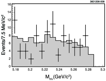
To avoid bias, we adopt a continuum smoothing procedure in which we reanalyze the off-resonance data with the explicit continuum suppression criteria removed. This procedure produces a relatively high-statistics set of $M_{h\ell\nu}-\Delta E$ distributions. We correct each distribution for potential bias caused by the removal of the continuum suppression. The correction is obtained from comparing analysis of an independent mock continuum sample with and without the continuum suppression criteria of our analysis. MC provides the $e^{+}e^{-}\to q\bar{q},\,\tau^{+}\tau^{-}$ component with true (generator-level) reconstructed leptons. The fake lepton component is obtained from sample of purely hadronic off-resonance data events combined with measured fake rates. After application of the bias correction, each distribution is normalized so that the integrated rate in the $M_{h\ell\nu}-\Delta E$ region input to the fit is identical to the integrated rate obtained from the off-resonance data with the continuum suppression. Figure 6 shows one example.

The off-resonance component is absolutely normalized in the fit based on the ratio of on- to off-resonance integrated luminosity with a correction for the energy dependence of the $e^{+}e^{-}\to q\bar{q}$ cross section.

Figure 6: The $M_{h\ell\nu}$ distribution for $B\to\pi\ell\nu$ candidates from off resonance data before (points with errors) and after (filled histogram) the continuum smoothing procedure.

4) $B\bar{B}$ Fake Signal Leptons: Both $B\bar{B}$ and continuum processes contribute backgrounds where a hadron has faked a lepton. Our continuum sample incorporates this contribution, but, as noted above, we do not rely on MC for the background component resulting from fake leptons.

We obtain the $B\bar{B}$ fake component from analysis of on-resonance and off-resonance data samples in which no leptons have been identified. For each reconstructed track satisfying our electron kinematic and fiducial criteria in each of these events, we analyze the event treating that track as the signal electron. If the event with that fake lepton candidate satisfies our analysis, then a contribution weighted by the measured electron fake rate for a track of that momentum is added. Each track is then similarly treated as a muon candidate. The on- and off-resonance samples are absolutely normalized in the fit based on luminosity. The off-resonance receives a negative normalization, causing the continuum component to be subtracted from the on-resonance data, thereby isolating the $B\bar{B}$ component.

5) Other $B\to X_{u}\ell\nu$ Decays: A final background arises from other $B\to X_{u}\ell\nu$ decays that we are not exclusively reconstructing in the fit. To model this background we use a hybrid exclusive-inclusive MC developed and documented by Meyer tomthesis that combines ISGW2 predictions of exclusive decays isgw2 with the inclusive lepton spectrum predicted using HQET by De Fazio and Neubert defazio . The parameters used in the heavy quark expansion are constrained by measurements of the $B\to X_{s}\gamma$ photon spectrum by CLEO cleobsgprl . The model generates resonant decays according to ISGW2 plus non-resonant decays such that the total generated spectrum matches theoretical predictions. We explicitly remove our exclusive decays from this simulation, and the remainder of the sample becomes the $B\to X_{u}^{\text{other}}\ell\nu$ component of the fit.

The normalization of this component uses a measurement of the inclusive charmless leptonic branching fraction by the BaBar collaboration babarinclep in the momentum endpoint range of 2.2 to 2.6 GeV$/c$. BaBar finds $\mathcal{B}(B\to X_{u}e^{+}\nu)_{\text{endpoint}}=(2.35\pm 0.22)\times 10^{-4}$. Roughly 10% of the generated $B\to X_{u}^{\text{other}}\ell\nu$ spectrum has a lepton in this range. For each iteration of the fit, we recalculate the normalization of the “Other $B\to X_{u}\ell\nu$” component so that the contributions of this component and of the seven signal modes to the endpoint region sum to the measured rate.

V.3 Verification of Fitting Procedure

To test the fitter for systematic biases, we performed a bootstrap study using 214 mock data samples which were generated by randomly selecting subsets of our MC events. For each mock sample, the numbers of events for each signal and background contribution were fixed to our efficiency–corrected yields. From fits to the 214 analyzed subsets, we find that the fitter reproduces the branching fractions without bias within the statistical uncertainties of the procedure (about 7% of the reported statistical error on a given quantity). Furthermore, the parametric uncertainties reported for the fits agree well with the widths of the distributions of the parameters’ central values.

The fit implementation was also cross-checked against an independent implementation used in the previous analysis bb:Athar:2003yg on that analysis’ data.

Table 4: A summary of the different components and the corresponding fill style in the subsequent histograms.

	signal		$B\to X_{u}\ell\nu$ other
	$\pi$ cross-feed		fake lepton
	$\rho/\omega$ cross-feed		continuum
	$\eta/\eta^{\prime}$ cross-feed		$b\to c$

V.4 Fit Results

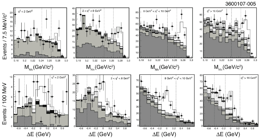
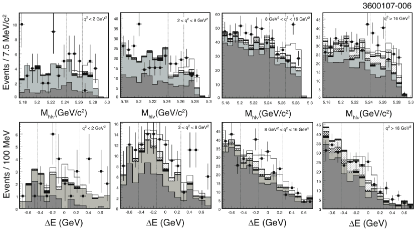
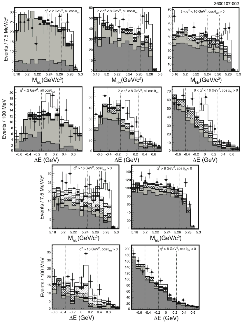
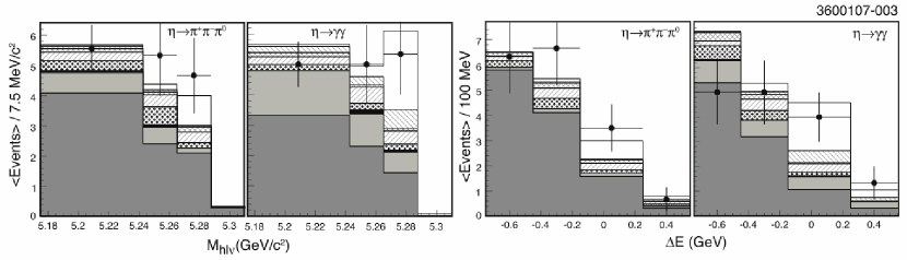
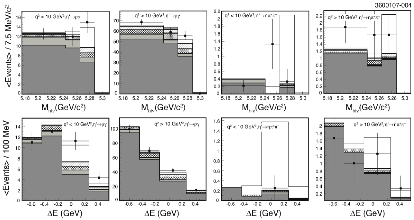
Table  5 summarizes the branching fractions obtained in the nominal fit for the $\pi\ell\nu$, $\rho\ell\nu$, $\eta\ell\nu$, and $\eta^{\prime}\ell\nu$ modes. The nominal fit converges with $-2\ln\mathcal{L}$ equal to 541 and we note that the statistical errors on some of the 532 bins are not Gaussian. Figures 7 - 11 show $M_{h\ell\nu}$ and $\Delta E$ projections for the nominal fit. These figures are generated by plotting $M_{h\ell\nu}$ for candidates with $\Delta E$ in the signal bin and vice versa. Note that for the $\pi$ and $\rho$ modes, the binning is finer than that which the fitter uses in order to show detailed peak structure. Raw signal yields for the various decay modes, integrated over phase space, are listed in Table 1.

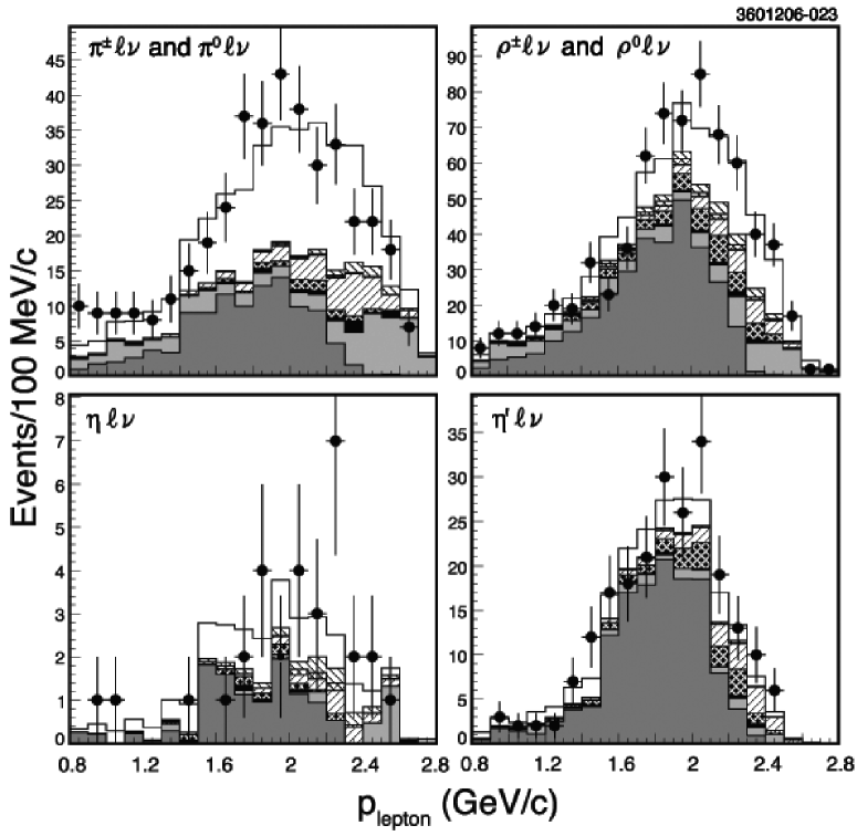
Figure 12 shows the lepton momentum spectrum for $B\to\pi\ell\nu$ and $B\to\rho\ell\nu$ events in the signal $\Delta E$–$M_{h\ell\nu}$ bin. As expected, the signal lepton spectrum for $B\to\rho\ell\nu$ is noticeably harder than that for $B\to\pi\ell\nu$. The agreement between the data and the sum of the fit components gives us confidence in the overall fit quality and our in ability to model the lepton momentum distribution of the fit components.

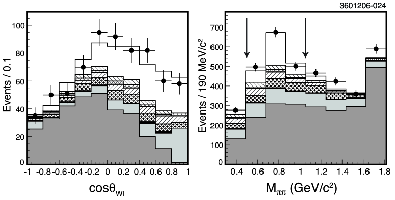
Figure 13 shows the projections of $\cos\theta_{Wl}$ and the invariant mass of the two pions, $M_{\pi\pi}$, used to construct the $\rho$ candidate for the $\rho\ell\nu$ modes. Again, the agreement between data and the sum of the fit components is excellent. In the $\cos\theta_{Wl}$ distribution the signal accumulates near one and the $b\to c$ background is concentrated in the area where $\cos\theta_{Wl}$ is less than zero as expected. The $M_{\pi\pi}$ projection shows a clear resonance component and extrapolates reliably into regions not used in the fit. The peak in the highest bin is due to $B\to D^{(*)}\ell\nu$ where the $D\to K\pi$ decay is identified as a $\rho\to\pi\pi$ decay.

Figure 7: The $M_{h\ell\nu}$ and $\Delta E$ projections of the nominal fit, $Q=0$, for the summed $\pi^{\pm}\ell\nu$ and $\pi^{0}\ell\nu$ modes. The fit components are described in Table 4.

Figure 8: The $M_{h\ell\nu}$ and $\Delta E$ projections of the nominal fit, $|Q|=1$, for the summed $\pi^{\pm}\ell\nu$ and $\pi^{0}\ell\nu$ modes. The fit components are described in Table 4.

Figure 9: The $M_{h\ell\nu}$ and $\Delta E$ projections of the nominal fit for the summed $\rho^{\pm}\ell\nu$ and $\rho^{0}\ell\nu$ modes. The fit components are described in Table 4.

Figure 10: The $M_{h\ell\nu}$ and $\Delta E$ projections of the nominal fit, $|Q|=0$, for the $\eta\ell\nu$ mode. The fit components are described in Table 4.

Figure 11: The $M_{h\ell\nu}$ and $\Delta E$ projections of the nominal fit, $|Q|=0$, for the $\eta^{\prime}\ell\nu$ mode. The fit components are described in Table 4. The $\eta^{\prime}\to\rho\gamma$ and $\eta^{\prime}\to\eta\pi\pi$ submodes have been summed.

Figure 12: Lepton momentum projections of the nominal fit for $\Delta Q=0$, $\pi^{\pm}\ell\nu$ and $\pi^{0}\ell\nu$ (top left), $\rho^{\pm}\ell\nu$ and $\rho^{0}\ell\nu$ (top right), $\eta\ell\nu$ (bottom left) and $\eta^{\prime}\ell\nu$ (bottom right). The data have been summed over $q^{2}$, $\cos\theta_{Wl}$, and, where applicable, decay mode.

Figure 13: The $\cos\theta_{Wl}$ projection of the nominal fit, summed over $q^{2}$, for the $\rho^{0}\ell\nu$ and $\rho^{\pm}\ell\nu$ modes (left). The projection of the two-pion invariant mass of the $\rho$ candidates summed over $q^{2}$ and $\cos\theta_{Wl}$ (right). Arrows indicate the region included in the fit. The peak at right is due to $B\to D^{(*)}\ell\nu$, with $D\to K\pi$ and the $K$ misidentified as a $\pi$.

Table 5: Summary of the phase space subregions and the partial and total branching fraction results. The errors shown are statistical and systematic, respectively.

	$q^{2}$ [GeV2]	$\cos\theta_{Wl}$	$\mathcal{B}$ [$10^{-4}$]
$B^{0}\to\pi^{-}\ell^{+}\nu$	0 - 2	${}^{-}1$ - 1	$0.13\pm 0.07\pm 0.02$
	2 - 8	${}^{-}1$ - 1	$0.27\pm 0.08\pm 0.03$
	8 - 16	${}^{-}1$ - 1	$0.56\pm 0.09\pm 0.05$
	$>16$	${}^{-}1$ - 1	$0.41\pm 0.08\pm 0.04$
	all phase space		${\bf 1.37\pm 0.15\pm 0.11}$
$B^{0}\to\rho^{-}\ell^{+}\nu$	0 - 2	${}^{-}1$ - 1	$0.45\pm 0.20\pm 0.15$
	2 - 8	${}^{-}1$ - 1	$0.96\pm 0.20\pm 0.29$
	8 - 16	0 - 1	$0.75\pm 0.16\pm 0.14$
	$>16$	0 - 1	$0.35\pm 0.07\pm 0.05$
	$>8$	${}^{-}1$ - 0	$0.42\pm 0.18\pm 0.31$
	all phase space		${\bf 2.93\pm 0.37\pm 0.37}$
$B^{0}\to\eta\ell^{+}\nu$	all phase space		${\bf 0.44\pm 0.23\pm 0.11}$
$B^{0}\to\eta^{\prime}\ell^{+}\nu$	all phase space		${\bf 2.66\pm 0.80\pm 0.56}$

VI Systematic Uncertainties

The systematic uncertainty in this analysis are dominated by effects that couple to accurate simulation of the missing momentum and energy used to reconstruct the neutrino, and to simulation of the selection criteria to isolate events where this association works well. Additional uncertainties enter from modeling of the background processes. We explicitly evaluate our residual uncertainty due to form factor shapes.

For most systematic effects, such as simulation of the absolute tracking efficiency, we have information from independent studies that limit their size. For most studies, statistics limit the sensitivity, so a Gaussian treatment is not unreasonable. To assess the effect of a given systematic on this analysis, we completely recreate the fit components with the suspect quantity biased to the limit of the study. This typically involves reweighting or biasing of the generated MC samples, which minimizes statistical issues in the determination of the shifts. For studies involving use of random numbers (e.g., discarding tracks to decrease the tracking efficiency), we repeat the study several times with different seeds to ensure that we have an accurate measure. We then refit, and assign the difference from the nominal fit as the systematic estimate. Note that we apply the bias to the same samples used to create the nominal fit components, which largely eliminates statistical fluctuations in the procedure.

This procedure will, in principle, cause compensating changes between the efficiencies input to the fit and the signal yields before efficiency correction obtained from the fit. Degrading resolution, for example, mainly smears signal out of the signal region (decreased efficiency), but allows greater latitude for backgrounds to smear into the signal region (increased background, so decreased signal yield). Since the systematic uncertainties can result in improper estimation of this cancellation, we will trust any cancellation to only 30% of itself, adding that portion back into the assessed uncertainty.

Because of correlations between yields in different regions of phase space, the systematic uncertainty for the total branching fraction can be smaller than uncertainties for the individual partial branching fractions.

VI.1 Systematic Uncertainties in Neutrino Reconstruction

The systematic uncertainties associated with neutrino reconstruction efficiency and resolution, summarized in Table 6, dominate the systematic uncertainties in this analysis.

Track Reconstruction Efficiency: Track reconstruction efficiency agrees in data and simulation to within 2.6% (5%) of itself for low momentum tracks (under 250 MeV$/c$) for CLEO II/II.5 (III) and to within 0.5% for high momentum tracks. We randomly discard tracks at these levels to assess the systematic effect. We conservatively assume that the uncertainties are fully correlated among the three detector configurations.

Track Momentum Resolution: Based on studies of the reconstructed $K\pi$ mass resolution in $D\to K\pi$ at the $\Upsilon(4S)$, we increase the deviations between reconstructed and generated track momenta by 10% (40%) in CLEO II/II.5 (III). The CLEO II/II.5 value is very conservative, while CLEO III value brings data and simulation into proper agreement.

Shower Reconstruction Efficiency: Shower reconstruction efficiency in data and simulation agree within 1.6% (1%) of itself for CLEO II/II.5 (III). We therefore randomly discard a fraction of the showers consistent with these limits. We again assume full correlation among different detector generations when modifying the simulation.

Shower Resolution: We increase all photon mismeasurements by 10% of themselves.

Hadronic Showering “Splitoff” Simulation and Rejection: We find that the number of splitoff clusters reconstructed from hadronic showers in our simulation deviate from the number in data by at most 0.03 per hadron. The energy spectrum agrees well. We therefore add additional showers with the observed spectrum at the rate of 0.03 per hadron in each event.

We also systematically distort the neural-net rejection variable, which is based upon shower shapes, until the data and simulation clearly disagree. We do this for both showers originating from photons and from hadronic shower simulations.

Particle Identification: Particle identification uncertainties directly affect the missing energy resolution. The device-based particle identification efficiencies are understood at the level of 5% or better, and our uncertainties as a function of detector and momentum are considered in our systematic evaluation. The overall effect of these uncertainties gets reduced by our weighting according to particle production probability.

$K^{0}_{L}$ Production and Energy Deposition: Our $K_{L}$ production rate correction is modified according to the statistical uncertainties of our $K_{S}$ data versus simulation study. A separate study of kaons that shower in the CsI calorimeter indicate that the deposited energy is simulated to within 20%.

Secondary Lepton Spectrum: We vary corrections based on the measurements of the inclusive $B\to D^{(*)}X$ spectrum and the electron momentum spectrum in inclusive semileptonic charm decay according to the envelope of potential $b\to c\to s\ell\nu$ lepton spectra resulting from the uncertainties in the spectral measurements.

Table 6: The systematic errors associated with neutrino reconstruction. Errors from different sources are assumed to be uncorrelated. The bottom row shows the quadrature-sum of the errors. The phase space interval indices are as defined in Table 2.

	$\delta\mathcal{B}\left(B^{0}\to\pi^{-}\ell^{+}\nu\right)~{}[\%]$						$\delta\mathcal{B}\left(B^{0}\to\rho^{-}\ell^{+}\nu\right)~{}[\%]$						$\delta\mathcal{B}\left(B^{+}\to(\eta/\eta^{\prime})\ell^{+}\nu\right)~{}[\%]$
Systematic Error Source	1	2	3	4	All		1	2	3	4	5	All	$\eta$	$\eta^{\prime}$
Track Efficiency	2.8	3.4	4.0	2.4	2.5		8.4	7.9	11.9	7.7	16.0	5.5	3.9	6.1
Track Resolution	1.7	2.1	1.8	2.7	1.4		10.3	16.2	0.8	2.8	50.0	1.0	6.3	9.6
Shower Efficiency	5.5	3.9	3.6	3.0	3.1		7.0	8.7	7.0	5.9	38.1	3.2	8.5	8.4
Shower Resolution	2.2	4.4	3.3	2.3	3.1		8.3	7.0	7.2	2.8	4.0	5.2	19.6	10.3
Splitoff Simulation	3.1	2.1	2.6	2.6	2.2		6.7	8.3	3.1	3.4	22.1	1.4	4.1	3.4
Splitoff Rejection	0.0	0.0	0.1	0.2	0.1		0.2	0.1	0.1	0.0	0.7	0.1	0.0	5.6
Particle Identification	0.7	2.2	0.9	4.4	1.1		7.5	12.7	0.8	3.4	18.0	2.4	2.5	3.5
$K^{0}_{L}$ Production	0.2	0.1	0.2	0.2	0.2		0.5	0.9	0.1	0.3	3.6	0.1	0.1	0.1
$K^{0}_{L}$ Energy Deposition	0.0	0.0	0.2	0.3	0.2		1.9	2.2	0.6	1.1	8.0	0.9	3.7	3.3
Secondary Lepton Spectrum	0.5	1.1	0.4	0.4	0.2		6.7	0.6	0.6	0.2	2.8	1.5	0.3	0.3
Sum	7.5	7.9	7.1	7.4	5.9		21.1	26.2	16.0	11.6	71.5	8.9	23.4	19.3

VI.2 Additional Sources of Systematic Error

The full list of systematic uncertainties are summarized in Table 7 and described below.

Continuum Suppression: We vary the independent parameters in the functions used in the continuum smoothing algorithm that parameterize the efficiency of our continuum suppression algorithm in the $M_{h\ell\nu}-\Delta E$ plane within their uncertainties.

$b\to c$: We vary the $B\to D\ell\nu$, $B\to D^{*}\ell\nu$, $B\to D^{**}\ell\nu$, and non-resonant $B\to X_{c}\ell\nu$ branching fractions according to the uncertainties obtained in Reference elliotprd . We also apply identical variations to the $B\to D^{*}\ell\nu$ form factors that are outlined in Reference elliotthesis .

Other $B\to X_{u}\ell\nu$: We vary the heavy quark expansion (HQE) parameters defazio at the heart of our hybrid $B\to X_{u}\ell\nu$ generator consistent with uncertainties in the CLEO $B\to X_{s}\gamma$ photon spectrum measurement cleobsgprl , which is conservative compared to current world knowledge. We also probe the hadronization uncertainty by changing the rate for the exclusive modes (not including our signal modes) by $\pm 10\%$, simultaneously adjusting the rate of the inclusively generated portion to maintain the same total rate.

We vary the endpoint rate to which our $B\to X_{u}\ell\nu$ component is fixed, within the uncertainties of the BaBar endpoint measurement babarinclep . All uncertainties are combined in the summary table, though the HQE and endpoint constraint uncertainties dominate.

Lepton Identification and Fake Leptons: We have measured our lepton identification efficiencies at the 2% level. We also vary the rate at which hadrons fake leptons by $\pm 50\%$. In momentum regions with measurable fake rates, this variation is very conservative.

$\pi^{0}$ Identification: The CLEO III MC simulation overestimates the $\pi^{0}$ efficiency by $4\pm 2\%$. Therefore we apply a correction of 0.96 to the CLEO III MC signal decays that contain a $\pi^{0}$ in the final state. Note that $\pi^{0}$ finding is only used in the process of reconstructing signal decays. To assess the systematic uncertainty, we remove this efficiency correction in CLEO III.

Number of $\Upsilon\to B\bar{B}$ Events: Based on luminosity, cross section, and event shape studies the error on the number of $B\bar{B}$ events in CLEO II + II.5 (III) is taken to be 2% (8%). Combining these uncertainties and accounting for the relative luminosities in each, we find an uncertainty on the total number of $B\bar{B}$ events, and therefore the branching fractions, to be 3.6%.

$\tau_{B^{+}}/\tau_{B^{0}}$ and $f_{+-}/f_{00}$: The fixed relative strengths of the charged and neutral rates are sensitive to both the lifetime and production ratios of charged and neutral $B$ mesons. Since the fit constraints on the charged and neutral $\pi$ and $\rho$ depend on $f_{+-}/f_{00}$, this systematic affects both the total yields from the fit and the conversion factor from the yields to branching fractions. We vary both the lifetime and production fraction ratios independently within the uncertainties produced by the Heavy Flavor Averaging Group hfag .

Final State Radiation: Final state radiation corrections calculated using PHOTOS photos are applied to the nominal results. We assign an uncertainty by varying final state radiation corrections by 20%.

Non-Resonant $B\to\pi\pi\ell\nu$: In the $B\to\rho\ell\nu$ modes there is an additional uncertainty from the unknown contribution of non-resonant $B\to\pi\pi\ell\nu$. Using isospin and angular momentum arguments outlined in bb:Athar:2003yg , we expect the dominant non-resonant $\pi\pi$ contribution to be in $\pi^{+}\pi^{-}$ and $\pi^{0}\pi^{0}$. While extracting a true non-resonant $\pi\pi\ell\nu$ yield is difficult with some knowledge of the form factors and mass distribution, we can limit the amount that a $\rho$ line shape can be projected out of the $\pi^{0}\pi^{0}\ell\nu$ data, and use the isospin relationships to, in turn, bound the non-resonant component in $\pi^{+}\pi^{-}\ell\nu$. Procedurally, we add the reconstructed $\pi^{0}\pi^{0}\ell\nu$ mode to the fit, and add one additional parameter that scales the non-resonant $\pi^{+}\pi^{-}\ell\nu$ and $\pi^{0}\pi^{0}\ell\nu$ rates. We find we could project out a yield, relative to the charged $\rho$ yield, of $-2.2\%\pm 6.2\%$, consistent with zero.

Table 7: A summary of the experimental systematic uncertainties. The bin numbers correspond to the $q^{2}$ and $\cos\theta_{Wl}$ intervals that were independently reconstructed in the fit. Errors from different sources are assumed to be uncorrelated. Neutrino reconstruction systematic errors are the totals summarized in Table 6. The phase space interval indices are as defined in Table 2.

	$\delta\mathcal{B}\left(B^{0}\to\pi^{-}\ell^{+}\nu\right)~{}[\%]$						$\delta\mathcal{B}\left(B^{0}\to\rho^{-}\ell^{+}\nu\right)~{}[\%]$						$\delta\mathcal{B}\left(B^{+}\to(\eta/\eta^{\prime})\ell^{+}\nu\right)~{}[\%]$
Systematic Error Source	1	2	3	4	All		1	2	3	4	5	All	$\eta$	$\eta^{\prime}$
Neutrino Reconstruction	7.5	7.9	7.1	7.4	5.9		21.1	26.2	16.0	11.6	71.5	8.9	23.4	19.3
Continuum Suppression	9.8	3.0	0.9	1.1	1.1		9.5	1.9	1.5	1.3	3.0	1.5	1.5	0.8
$B\to X_{c}\ell\nu$	4.0	3.9	1.3	1.2	1.5		20.8	12.2	2.7	2.2	12.7	5.8	2.1	4.8
Other $B\to X_{u}\ell\nu$	2.3	1.2	2.3	5.8	2.5		5.8	3.6	7.4	3.7	17.0	2.8	3.5	3.0
Fake Leptons	4.9	1.3	2.3	0.6	1.7		3.1	2.5	1.0	1.1	4.5	1.1	1.1	3.7
Lepton Identification	2.0	2.0	2.0	2.0	2.0		2.0	2.0	2.0	2.0	2.0	2.0	2.0	2.0
$\pi^{0}$ Identification	0.3	0.3	0.2	0.2	0.1		1.0	0.9	1.3	0.9	3.3	1.4	0.2	0.1
Number of $\Upsilon\to B\bar{B}$	3.6	3.6	3.6	3.6	3.6		3.6	3.6	3.6	3.6	3.6	3.6	3.6	3.6
$\tau_{B^{+}}/\tau_{B^{0}}$	0.5	0.3	0.4	0.4	0.4		0.8	0.7	0.6	0.8	0.5	0.7	0.2	0.2
$f_{+-}/f_{00}$	0.5	0.9	0.7	0.8	0.7		0.1	0.0	0.2	0.2	0.6	0.1	2.1	2.0
Non-Resonant $\pi\pi$	1.9	2.0	0.4	0.6	0.6		5.1	3.6	2.1	3.2	3.9	3.5	2.0	2.1
Final State Radiation	1.6	1.0	1.0	1.1	1.1		1.2	1.5	2.2	1.8	2.0	1.8	1.2	1.6
Sum	14.8	10.6	9.1	10.5	8.2		32.5	29.8	18.7	13.7	75.3	12.6	24.4	21.2

VI.3 Dependence on Form Factors

The previous CLEO measurement of the $B\to\pi\ell\nu$ and $B\to\rho\ell\nu$ rates achieved a very minimal dependence on a priori form factors for $B\to\pi\ell\nu$ by measuring independent rates in $q^{2}$ intervals similar to those in this analysis. Significant dependence on the $B\to\rho\ell\nu$ form factor, however, remained. Adding the $\cos\theta_{Wl}<0$ information in this analysis has greatly reduced this residual dependence.

To evaluate the dependence on the form factors, we choose a set of calculations that span the a very conservative range of theoretical results. For each form factor, we re-weight our signal MC and refit to assess the impact of the change. We vary the $B\to\pi\ell\nu$ and $B\to\rho\ell\nu$ form factors independently. For each of those, we assign a systematic contribution for the rate in each measured phase space region to be $1/2$ the difference of the largest and smallest rates obtained in that region for the different form factors. The systematic errors due to uncertainties in the signal decay form factors are summarized in Table 8.

For $B\to\pi\ell\nu$, we consider form factors from the unquenched lattice QCD calculations by HPQCD HPQCD_2006 (our nominal form factor), from Ball and Zwicky ball_2005 , Scora and Isgur (ISGW2) isgw2 , and Feldmann and Kroll spd . The variation in $q^{2}$ dependence of the rate from these calculations is illustrated in Figure 1.

For $B\to\rho\ell\nu$, we consider the Ball and Zwicky LCSR calculation (our nominal form factors), as well as those of Melikhov and Stech meli , from the quenched lattice calculations of UKQCD ukqcd98 , and from Scora and Isgur (ISGW2) isgw2 . Figure 2 shows the the calculated rates as a function of $q^{2}$ and $\cos\theta_{Wl}$. Note that the variation between calculations for the rate as a function of $\cos\theta_{Wl}$ is significant, which led to the remaining model dependence of the previous analysis.

Our main sensitivity in the $B^{+}\to\eta^{\prime}\ell^{+}\nu$ mode comes from the $q^{2}<10$ GeV² region, increasing our sensitivity to this mode’s form factor shape. We assess this sensitivity by varying the fraction of the $B\to\eta^{\prime}\ell\nu$ rate with $q^{2}<10$ GeV² by $\pm 10\%$ of itself.

Table 8: The systematic uncertainties associated with the individual form factor uncertainties are listed below. The numbers correspond to the $q^{2}$ and $\cos\theta_{Wl}$ intervals that were independently reconstructed in the fit. The phase space interval indices are as defined in Table 2.

	$\delta\mathcal{B}\left(B^{0}\to\pi^{-}\ell^{+}\nu\right)~{}[\%]$						$\delta\mathcal{B}\left(B^{0}\to\rho^{-}\ell^{+}\nu\right)~{}[\%]$						$\delta\mathcal{B}\left(B^{+}\to(\eta/\eta^{\prime})\ell^{+}\nu\right)~{}[\%]$
Form Factor	1	2	3	4	All		1	2	3	4	5	All	$\eta$	$\eta^{\prime}$
$B\to\pi\ell\nu$	1.2	0.5	0.5	2.8	0.8		0.3	0.3	0.7	0.3	2.1	0.4	0.3	0.2
$B\to\rho\ell\nu$	0.4	0.5	1.1	1.0	0.8		2.9	4.9	0.9	1.8	7.0	1.8	0.3	1.6
$B\to\eta^{\prime}\ell\nu$	0.1	0.2	0.2	0.7	0.3		0.9	1.5	1.1	0.9	5.2	0.5	0.3	1.4

VII Discussion of Results

VII.1 $|V_{ub}|$

Extraction of $|V_{ub}|$ from a measured $B\to X_{u}\ell\nu$ rate requires theoretical input in the form of the form factor(s) governing their decay. The unquenched LQCD calculations for the $B\to\pi\ell\nu$ form factor make a minimal number of assumptions. Therefore, our primary result for $|V_{ub}|$ derives from our $B\to\pi\ell\nu$ measurement in combination with LQCD results. The $\rho$ is unstable in unquenched lattice calculations, resulting in a multibody hadronic final state that current lattice technology is unable to accommodate. Our primary result for $B\to\rho\ell\nu$ is a validation of the form factor shapes needed to control the $\rho\ell\nu$ backgrounds in other $B\to\pi\ell\nu$ measurements.

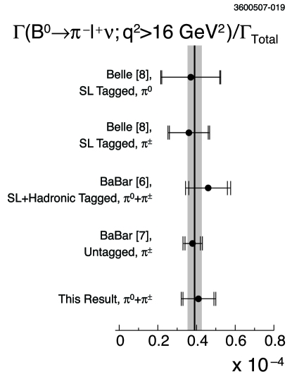
A determination of $|V_{ub}|$ from our $B\to\pi\ell\nu$ results will be most competitive if the full range of $q^{2}$ can be utilized. However, unquenched LQCD calculations currently cover the range $q^{2}>16~{}\text{GeV}^{2}$ HPQCD_2006 . The experimental constraints on the form factor shape do allow for useful extrapolation of the LQCD results outside this region Arnesen:2005ez ; Becher:2005bg , but techniques for optimal use of both the experimental and LQCD information are still under development Gibbons06 . Unquenched lattice calculations that utilize a moving $B$ meson frame to extend the $q^{2}$ range Davies:2006aa are also under development, but not yet complete. We therefore currently limit ourselves to the range $q^{2}>16~{}\text{GeV}^{2}$, for which the HPQCD collaboration finds $\Gamma(B^{0}\to\pi^{-}\ell^{+}\nu;\,q^{2}>16~{}\text{GeV}^{2})=|V_{ub}|^{2}(2.07\pm 0.41\pm 0.39\text{~{}ps}^{-1})$ HPQCD_2006 . Using a $B^{0}$ meson lifetime of $1.53\times 10^{-12}$ s pdg06 , we find $|V_{ub}|=\left(3.6\pm 0.4\pm 0.2^{+0.6}_{-0.4}\right)\times 10^{-3}$. The errors are, in order, statistical, experimental systematic, and theoretical systematic, where the final theoretical systematic error is driven by the expected uncertainty in the normalization of the form factor as calculated by our chosen LQCD calculation.

Figure 14 summarizes the current measurements by both Belle bb:BELLEy2007 and BaBar bb:BABARy2006 ; bb:BABARy2007 along with the results presented in this analysis for the $q^{2}>16~{}\text{GeV}^{2}$ region. There very good agreement among the various results and analysis techniques for partial branching fraction in this region of phase space which is currently the key experimental input to determinations of $|V_{ub}|$ using unquenched LQCD calculations.

Figure 14: A comparison of the current measurements of the $B^{0}\to\pi^{-}\ell^{+}\nu$ partial branching fraction in the $q^{2}>16$ GeV² region. The inner (outer) error bars are statistical (statistical and systematic). Results from Belle bb:BELLEy2007 use semleptonic $B$ decay to tag the non-signal $B$. BaBar has published results for an analysis bb:BABARy2006 using hadronic and semileptonic $B$ decays to tag the non-signal $B$ and also an analysis bb:BABARy2007 utilizing loose $\nu$ reconstruction. Where applicable $B^{0}\to\pi^{-}\ell^{+}\nu$ and $B^{+}\to\pi^{0}\ell^{+}\nu$ results have been averaged assuming isospin symmetry. A weighted average and one standard-deviation error band, assuming uncorrelated errors, are shown.

VII.2 $B\to\rho\ell\nu$ Form Factors

For $B\to\rho\ell\nu$, we perform a single-parameter fit to our measurements over the $\rho$ phase space for the ISGW2 isgw2 , LCSR ball_2005 , and quenched LQCD DelDebbio:1997kr (qLQCD) calculations. The LCSR results are the results most heavily relied upon for simulation of the $\rho\ell\nu$ background to $\pi\ell\nu$. The calculation is expected to be valid for the region $q^{2}\lesssim 14~{}\text{GeV}^{2}$. We therefore fit this calculation both to our measurements spanning the full $q^{2}-\cos\theta_{Wl}$ range and to our three subregions (see Table 5) that are restricted to $q^{2}<16~{}\text{GeV}^{2}$. The full phase space fits test the validity of a given model for use as a background model. The restricted phase space fit for LCSR tests the shape without extrapolation outside its region of validity. The results are summarized in Table 9. All of the probabilities of $\chi^{2}$ exceed 10% for the LCSR and LQCD, indicating reasonable agreement between theory and experiment at our current precision. The ISGW II model has only a 5% probability. While these constitute the most stringent tests to date of the $B\to\rho\ell\nu$ shape predictions, we cannot yet experimentally distinguish between the published central LCSR values and the effective shape variations used for background systematics in the recent BaBar $B\to\pi\ell\nu$ measurement bb:BABARy2007 .

Table 9: Summary of $\chi^{2}$ and number of degrees of freedom ($N_{\text{dof}}$) for fits to the $B\to\rho\ell\nu$ differential rate.

Form Factor	Phase Space	$\chi^{2}$	$N_{\text{dof}}$
ISGW II	full	9.0	4
LCSR	full	4.5	4
LCSR	restricted	4.3	2
LQCD	full	4.3	4

VII.3 $\mathcal{B}(B^{+}\to\eta\ell^{+}\nu)$ and $\mathcal{B}(B^{+}\to\eta^{\prime}\ell^{+}\nu)$

We do not see a statistically significant signal in the $B\to\eta\ell\nu$ mode. When ${\cal B}(B^{+}\to\eta\ell^{+}\nu)$ is forced to zero, $-2\ln{\cal L}$ increases by 4.8, which corresponds to less than a three standard deviation effect. While less statistically significant than reported by the previous analysis, the yields in the new relative to the old dataset are consistent within statistical errors.

Forcing ${\cal B}(B^{+}\to\eta^{\prime}\ell^{+}\nu)=0$, $-2\ln{\cal L}$ increases by 17.9, but we must fold in systematic uncertainties to evaluate the significance. Taking the systematic uncertainties as Gaussian, we convolute them with our statistical probability distribution function (p.d.f.) inferred from the $-2\ln{\cal L}$ distribution of the fit to model the total p.d.f.. From a toy MC based on this p.d.f., we determine the probability for measuring a rate greater than or equal to our central value, if the true rate were zero, to be $1.2\times 10^{-3}$. Therefore, we interpret the significance of our signal to be just over a three standard deviations.

Using the procedure just described, we find the 90% confidence interval of $1.20\times 10^{-4}<{\cal B}(B^{+}\to\eta^{\prime}\ell^{+}\nu)<4.46\times 10^{-4}$. For $B\to\eta\ell\nu$, we obtain a 90% confidence level upper limit of ${\cal B}(B^{+}\to\eta\ell^{+}\nu)\leq 1.01\times 10^{-4}$. We also determine the lower limit for the ratio ${\cal B}(B^{+}\to\eta^{\prime}\ell^{+}\nu)/{\cal B}(B^{+}\to\eta\ell^{+}\nu)$ to be 2.5 at the 90% confidence level.

Our results allow us to make some model dependent statements regarding the size of the extra gluon couplings from the $\eta^{0}$ singlet component of the $\eta$ and $\eta^{\prime}$. Beneke and Neubert use the Feldmann, Kroll, and Stech (FKS) mixing scheme etap:FKS in an analysis of $B\to\eta^{\prime}X_{s}$ etap:Neubert2003 to model the $B\to\eta^{(\prime)}$ form factors as

$$F^{B\to\eta^{(\prime)}}_{+}=F^{B\to\pi}_{+}\frac{f^{q}_{\eta^{(\prime)}}}{f_{\pi}}+F^{\text{singlet}}_{+}\frac{\sqrt{2}f^{q}_{\eta^{(\prime)}}+f^{s}_{\eta^{(\prime)}}}{\sqrt{3}f_{\pi}},$$ (5)

where $F^{B\to\pi}$ is the $B\to\pi$ form factor, $F^{\text{singlet}}$ is an unknown singlet component, and $f^{(q,s)}_{\eta^{(\prime)}}$ are constants determined by the FKS mixing scheme. Kim etap:CSK recognized that comparison of $B$ decay to $\eta\ell\nu$ and $\eta^{\prime}\ell\nu$ could determine the size of the singlet component.

With the model-dependent parameter

$$\tilde{F}_{s}=\frac{\int|F^{\text{singlet}}_{+}|^{2}\Omega_{\eta^{\prime}}\partial q^{2}}{\int|F^{B\to\pi}_{+}|^{2}\Omega_{\eta^{\prime}}\partial q^{2}},$$ (6)

where $\Omega_{\eta^{\prime}}$ is the appropriate phase space factor, the $B^{+}\to\eta^{(\prime)}\ell^{+}\nu$ to $B^{+}\to\pi^{0}\ell^{+}\nu$ branching ratios may be expressed as

$$\frac{{\cal B}_{\eta^{\prime}}}{2{\cal B}_{\pi^{0}}} = \beta_{\eta^{\prime}}\left(a_{\eta^{\prime}}^{2}+2\gamma_{\eta^{\prime}}a_{\eta^{\prime}}b_{\eta^{\prime}}\sqrt{\tilde{F}_{s}}+\tilde{F}_{s}b_{\eta^{\prime}}^{2}\right)$$ (7)

$$\frac{{\cal B}_{\eta}}{2{\cal B}_{\pi^{0}}} = \beta_{\eta}\left(a_{\eta}^{2}+2\gamma_{\eta}a_{\eta}b_{\eta}\sqrt{\tilde{F}_{s}\frac{\beta_{\eta^{\prime}}}{\beta_{\eta}}t}+\tilde{F}_{s}\frac{\beta_{\eta^{\prime}}}{\beta_{\eta}}tb_{\eta}^{2}\right).$$

The parameters $a_{\eta^{(\prime)}}$ and $b_{\eta^{(\prime)}}$ are combinations of FKS mixing parameters, while $\beta_{\eta^{(\prime)}}$, $\gamma_{\eta^{(\prime)}}$ and $t$ capture differences in the $F^{\pi}_{+}$ and $F^{\text{singlet}}_{+}$ $q^{2}$ dependence. Following Kim, we assume that the $F^{B\to\pi}$ and $F^{\text{singlet}}$ have the same $q^{2}$ dependence, and cover shape differences with a systematic uncertainty.

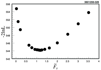
We impose these branching ratio relationships in our standard fitting procedure and allowing $\tilde{F}_{s}$ to float as a free parameter. We find $\tilde{F}_{s}=1.15\pm 0.54\pm 0.38\pm 0.21$, where the errors listed are, in order, statistical, systematic, and those due to uncertainties related to this model, including the relative $q^{2}$ dependence. The variation of the likelihood with $\tilde{F}_{s}$ is shown in Figure 15. The $B\to\eta^{(\prime)}\ell\nu$ branching fractions found with this model are consistent with the results of our nominal fit.

Figure 15: The change in the $-2\ln{\cal L}$ of the fit as a function of the parameter $\tilde{F}_{s}$.

With our $\tilde{F}_{s}$ determination, we can roughly update the $B^{-}\to K^{-}\eta^{\prime}$ prediction of Benke and Neubert by scaling their $F^{\text{singlet}}(q^{2}=0)=0.1$ (about equivalent to $\tilde{F}_{s}\sim 0.137$) result, for which they found ${\cal B}(B^{-}\to K^{-}\eta^{\prime})=(56^{+19}_{-14}{}^{+31}_{-13})\times 10^{-6}$. Experimentally, ${\cal B}(B^{-}\to K^{-}\eta^{\prime})=(71\pm 4)\times 10^{-6}$ pdg06 . With our $\tilde{F}_{s}$, we estimate ${\cal B}(B^{-}\to K^{-}\eta^{\prime})=(84^{+35}_{-25}{}^{+53}_{-24})\times 10^{-6}$, though a rigorous calculation with $\tilde{F}_{s}\sim 1$ is needed. This estimate is double the prediction with no singlet contribution and agrees well with the experimental value.

VIII Summary

We have measured the branching fractions $\mathcal{B}\left(B^{0}\to\pi^{-}\ell^{+}\nu\right)=(1.37\pm 0.15\pm 0.11)\times 10^{-4}$ and $\mathcal{B}\left(B^{0}\to\rho^{-}\ell^{+}\nu\right)=(2.93\pm 0.37\pm 0.37)\times 10^{-4}$ with very little residual dependence of either branching fraction on either the $B\to\pi$ or $B\to\rho$ form factors. Table 5 summarizes the branching fraction results for the partial phase space measurements that are summed to obtain the measurements integrated over phase space. These results agree well with recent measurements from BaBar bb:BABARy2005 ; bb:BABARy2006 ; bb:BABARy2007 and Belle bb:BELLEy2007 . The total branching fractions for the $\pi\ell\nu$ and $\rho\ell\nu$ modes are among the most precise current measurements. These results indicate that at the level of experimental precision we can probe, the $B\to\rho\ell\nu$ form factor shapes obtained with LCSR agree with our data, though we cannot test the shape at the uncertainty level assumed in the BaBar $B\to\pi\ell\nu$ analysis bb:BABARy2007 . Using the most recent unqenched lattice QCD calculations of the $B\to\pi\ell\nu$ form factor HPQCD_2006 , and measured rate for $q^{2}>16~{}\text{GeV}^{2}$ region we extract $|V_{ub}|=(3.6\pm 0.4\pm 0.2^{+0.6}_{-0.4})\times 10^{-3}$, where the uncertainties are statistical, experimental, and theoretical, respectively. While this value is competitive with other recent determinations of $|V_{ub}|$, the full strength of this analysis will be more effectively realized when a broader $q^{2}$ range can be used reliably for the determination of $|V_{ub}|$.

We find evidence for $B^{+}\to\eta^{\prime}\ell^{+}\nu$ at the three standard deviation level with a branching fraction of ${\cal B}(B^{+}\to\eta^{\prime}\ell^{+}\nu)=(2.66\pm 0.80\pm 0.56)\times 10^{-4}$ and a 90% confidence interval of $1.20\times 10^{-4}<{\cal B}(B^{+}\to\eta^{\prime}\ell^{+}\nu)<4.46\times 10^{-4}$. The probability that our results for $\mathcal{B}\left(B^{+}\to\eta^{\prime}\ell^{+}\nu\right)$ are consistent with a previous 90% confident limit set by BaBar BaBar_eta_ichep06 of $1.3\times 10^{-4}$ is approximately 5%. We establish an upper limit for the $B^{+}\to\eta\ell^{+}\nu$ branching fraction of ${\cal B}(B^{+}\to\eta\ell^{+}\nu)\leq 1.01\times 10^{-4}$ (90% confidence level), with systematic uncertainties included. This is consistent with the BaBar 90% confident upper limit BaBar_eta_ichep06 of $1.4\times 10^{-4}$. These results imply a lower limit of ${\cal B}(B^{+}\to\eta^{\prime}\ell^{+}\nu)/{\cal B}(B^{+}\to\eta\ell^{+}\nu)>2.5$ (90% confidence level). Furthermore, the relative rates indicate a significant form factor contribution from the singlet component of the $\eta^{\prime}$, which can bring predictions for ${\cal B}(B\to K^{-}\eta^{\prime})$ into better agreement with experimental measurements.

These results supersede those previously published by CLEO bb:Athar:2003yg . While some shifts of central values are observed, particularly for $B^{0}\to\rho^{-}\ell\nu$, these results are consistent within statistical and systematic errors of those previously presented. We note that retuning of the event selection algorithm at low $q^{2}$ significantly reduces the statistical and systematic correlation between results in this region of phase space. Furthermore, expanding the measured $B\to\rho\ell\nu$ phase space nearly eliminates the theoretical systematic errors due to the $B\to\rho$ form factor uncertainty that were a significant contribution to the total error on the previous result.

To allow external use of our data in form factor, $|V_{ub}|$, and $\eta$ and $\eta^{\prime}$ isosinglet studies, we provide the full statistical and systematic uncertainty correlation matrices in Appendix A.

We gratefully acknowledge the effort of the CESR staff in providing us with excellent luminosity and running conditions. D. Cronin-Hennessy and A. Ryd thank the A.P. Sloan Foundation. This work was supported by the National Science Foundation, the U.S. Department of Energy, and the Natural Sciences and Engineering Research Council of Canada.

IX Appendix: Full Correlation Matrices

Tables 10 and 11 provide the correlation matrices for both the statistical and systematic errors on the branching fractions outlined in Table 5. Cross-feed among bins produces anti-correlations in the results for individual bins; therefore, techniques for extracting $|V_{ub}|$ by averaging over multiple bins in the fit tend to have reduced uncertainty when these correlations are taken into account.

Table 10: The statistical correlation matrix for the measured branching fractions. The phase space interval indices are as defined in Table 2.

Mode	Index
$\pi$	1	1.000	-0.098	0.001	-0.003	-0.002	0.004	-0.158	0.036	0.008	0.007	0.003
$\pi$	2	-0.098	1.000	-0.040	0.001	-0.007	0.012	-0.015	-0.195	0.037	-0.003	0.007
$\pi$	3	0.001	-0.040	1.000	-0.020	-0.025	0.013	0.003	-0.071	-0.173	0.089	-0.105
$\pi$	4	-0.003	0.001	-0.020	1.000	-0.054	0.018	-0.013	-0.019	-0.015	-0.345	-0.172
$\eta$	–	-0.002	-0.007	-0.027	-0.054	1.000	-0.008	-0.001	0.002	0.012	-0.058	-0.059
$\eta^{\prime}$	–	0.004	0.012	0.013	0.018	-0.008	1.000	-0.010	-0.054	-0.043	0.004	-0.113
$\rho$	1	-0.158	-0.015	0.003	-0.013	-0.001	-0.010	1.000	-0.151	0.031	-0.007	0.048
$\rho$	2	0.036	-0.195	-0.071	-0.019	0.002	-0.054	-0.151	1.000	0.027	0.063	0.102
$\rho$	3	0.008	0.037	-0.173	-0.015	0.012	-0.043	0.031	0.027	1.000	-0.126	0.036
$\rho$	4	0.007	-0.003	0.089	-0.345	-0.058	0.004	-0.007	0.063	-0.126	1.000	-0.267
$\rho$	5	0.003	0.007	-0.105	-0.172	-0.059	-0.113	0.048	0.102	0.036	-0.267	1.000

Table 11: The systematic correlation matrix for the measured branching fractions. The phase space interval indices are as defined in Table 2.

Mode	Index
$\pi$	1	1.000	0.674	0.678	0.383	0.388	-0.033	0.501	0.373	0.337	0.406	-0.257
$\pi$	2	0.674	1.000	0.754	0.115	0.575	-0.000	0.279	0.012	0.604	0.661	0.246
$\pi$	3	0.678	0.754	1.000	0.588	0.502	-0.016	0.368	0.258	0.536	0.514	0.056
$\pi$	4	0.383	0.115	0.588	1.000	0.407	-0.340	0.563	0.704	0.111	-0.099	-0.542
$\eta$	–	0.388	0.575	0.502	0.407	1.000	-0.665	0.416	0.406	0.587	0.260	-0.299
$\eta^{\prime}$	–	-0.033	-0.000	-0.016	-0.340	-0.665	1.000	-0.285	-0.477	-0.232	0.228	0.571
$\rho$	1	0.501	0.279	0.368	0.563	0.416	-0.285	1.000	0.852	0.200	0.110	-0.580
$\rho$	2	0.373	0.012	0.258	0.704	0.406	-0.477	0.852	1.000	0.136	-0.159	-0.831
$\rho$	3	0.337	0.604	0.536	0.111	0.587	-0.232	0.200	0.136	1.000	0.737	0.141
$\rho$	4	0.406	0.661	0.514	-0.099	0.260	0.228	0.110	-0.159	0.737	1.000	0.442
$\rho$	5	-0.257	0.246	0.056	-0.542	-0.299	0.571	-0.580	-0.831	0.141	0.442	1.000

References

- (1) N. Cabibbo, Phys. Rev. Lett. 10, 531 (1963); M. Kobayashi and T. Maskawa, Prog. Theor. Phys. 49, 652 (1973).
- (2) J. P. Alexander et al. [CLEO Collaboration], Phys. Rev. Lett. 77, 5000 (1996).
- (3) B. H. Behrens et al. [CLEO Collaboration], Phys. Rev. D 61, 052001 (2000).
- (4) S. B. Athar et al. [CLEO Collaboration], Phys. Rev. D 68, 072003 (2003).
- (5) B. Aubert et al. [BaBar Collaboration], Phys. Rev. D 72, 051102 (2005).
- (6) B. Aubert et al. [BaBar Collaboration], Phys. Rev. Lett. 97, 211801 (2006).
- (7) B. Aubert et al. [BaBar Collaboration], Phys. Rev. Lett. 98, 091801 (2007).
- (8) T. Hokuue et al. [Belle Collaboration], Phys. Lett. B 648, 139 (2007).
- (9) R. Kowalewski and T. Mannel, Determination of and , in Review of Particle Properties, W.-M. Yao et al. [Particle Data Group], J. Phys. G 33, 1 (2006).
- (10) E. Gulez et al. [HPQCD Collaboration], Phys. Rev. D 73, 074502 (2006); Erratum: submitted to Phys. Rev. D, [arXiv:hep-lat/0601021].
- (11) P. Ball and R. Zwicky, Phys. Rev. D 71, 014015 (2005).
- (12) P. Ball and R. Zwicky, Phys. Rev. D 71, 014029 (2005).
- (13) T. Feldmann, P. Kroll and B. Stech, Phys. Rev. D 58, 114006 (1998).
- (14) S. J. Richichi et al. [CLEO Collaboration], Phys. Rev. Lett. 85, 520 (2000).
- (15) B. Aubert et al. [BaBar Collaboration], Phys. Rev. Lett. 91, 161801 (2003).
- (16) K. Abe et al. [Belle Collaboration], Phys. Lett. B 517, 309 (2001).
- (17) B. Aubert et al. [BaBar Collaboration], Proceedings of the 33rd International Conference on High Energy Physics (ICHEP 06), [arXiv:hep-ex/0607066].
- (18) M. R. Shepherd, Ph.D. thesis, Cornell University, (2005), unpublished.
- (19) F. J. Gilman and R. L. Singleton, Jr. , Phys. Rev. D 41, 142 (1990).
- (20) T. Feldmann and P. Kroll, Eur. Phys. J. C 12, 99 (2000).
- (21) D. Scora and N. Isgur, Phys. Rev. D 52, 2783 (1995).
- (22) D. Melikhov and B. Stech, Phys. Rev. D 62, 014006 (2000).
- (23) L. Del Debbio et al. [UKQCD Collaboration], Phys. Lett. B 416, 392 (1998).
- (24) F. Wurthwein, Presented at 32nd Rencontres de Moriond: QCD and High-Energy Hadronic Interactions, Les Arcs, France, March 1997, [arXiv:hep-ex/9706010].
- (25) M. Artuso et al. [CLEO Collaboration], Phys. Rev. D 67, 052003 (2003)
- (26) See, for example, M. Peskin and D. Schroeder, An Introduction to Quantum Field Theory, Persus Books Publishing L.L.C., p.673 (1995).
- (27) C. S. Kim, S. Oh and C. Yu, Phys. Lett. B 590, 223 (2004).
- (28) Y. Kubota et al. [CLEO Collaboration], Nucl. Instrum. Meth. A 320, 66 (1992).
- (29) T. S. Hill et al. [CLEO Collaboration], Nucl. Instrum. Meth. A 418, 32 (1998).
- (30) D. Peterson et al. [CLEO Collaboration], Nucl. Instrum. Meth. A 478, 145 (2002).
- (31) M. Artuso et al., Nucl. Instrum. Meth. A 554, 147 (2005).
- (32) R. A. Fisher, Annals of Eugenics 7, 179 (1936).
- (33) G. C. Fox and S. Wolfram, Phys. Rev. Lett. 41, 1581 (1978).
- (34) R. J. Barlow and C. Beeston, Comput. Phys. Commun. 77, 219 (1993).
- (35) R. Brun et al., Geant 3.21, CERN Program Library Long Writeup W5013 (1993), unpublished.
- (36) S. E. Csorna et al. [CLEO Collaboration], Phys. Rev. D 70, 032002 (2004).
- (37) W. M. Yao et al. [Particle Data Group], J. Phys. G 33, 1 (2006).
- (38) L. Gibbons et al. [CLEO Collaboration], Phys. Rev. D 56, 3783 (1997).
- (39) N. E. Adam et al. [CLEO Collaboration], Phys. Rev. Lett. 97, 251801 (2006).
- (40) J. Alexander et al., [Heavy Flavor Averaging Group (HFAG)], 2005, [arXiv:hep-ex/0412073].
- (41) E. Barberio, B. van Eijk, Z. Was, Comput. Phys. Commun. 66, 115 (1991); E. Barberio and Z. Wa̧s, Comput. Phys. Commun. 79, 291 (1994).
- (42) T. O. Meyer, Ph.D. thesis, Cornell University (2005), unpublished.
- (43) F. De Fazio and M. Neubert, JHEP 9906, 017 (1999).
- (44) S. Chen et al. [CLEO Collaboration], Phys. Rev. Lett. 87, 251807 (2001).
- (45) B. Aubert et al. [BaBar Collaboration], Phys. Rev. D 73, 012006 (2006).
- (46) E. Lipeles, Ph.D. thesis, California Institute of Technology (2003), unpublished.
- (47) C. M. Arnesen, B. Grinstein, I. Z. Rothstein and I. W. Stewart, Phys. Rev. Lett. 95, 071802 (2005).
- (48) T. Becher and R. J. Hill, Phys. Lett. B 633, 61 (2006).
- (49) L. Gibbons, Presented at Beauty 2006: The 11th International Conference on B-Physics at Hadron Machines, Oxford, UK, Sept. 2006.
- (50) C. T. H. Davies, K. Y. Wong and G. P. Lepage, Presented at 24th International Symposium on Lattice Field Theory (Lattice 2006), Tucson, AZ, July 2006, [arXiv:hep-lat/0611009].
- (51) L. Del Debbio, J. M. Flynn, L. Lellouch, and J. Nieves [UKQCD Collaboration], Phys. Lett. B 416, 392 (1998).
- (52) M. Beneke and M. Neubert, Nucl. Phys. B 651, 255 (2003).