SLAC-R-860

XXXX

Review of Exclusive $B\rightarrow D^{(*,**)}l\nu$ Decays – Branching Fractions, Form-factors and $|V_{cb}|$

Contribution to the Proceedings of HQL06,
Munich, October 16th-20th, 2006

A. E. Snyder
Stanford Linear Accelerator Center (SLAC)
Menlo Park, CA, USA 94041

1 Introduction

This paper reviews semileptonic decays of $B$-mesons to states containing charm mesons, i.e., $D$,  $D^{*}$, $D^{**}$ and possible non-resonant $D^{(*)}n\pi$ states as well. The paper covers measurement of branching fractions, form-factors and, most importantly, the magnitude of the CKM matrix element $V_{cb}$.

I will not attempt a comprehensive review, but will concentrate on reasonably fresh results and consider mostly exclusive measurements. I will also comment on the consistency of the results and what needs to be done to resolve the apparent conflicts.

2 Physics and motivation

At the parton level (see Figure 1) the decay rate is simply related to $|V_{cb}|$ by

$$\Gamma=\frac{G_{F}^{2}}{192\pi^{3}}m_{b}^{5}|V_{cb}|^{2}$$ (1)

at tree level. A slightly more complicated formula applies if higher order QCD (loop corrections) are considered [1]. It’s still thought to be theoretical clean at the parton level, but the parton level process cannot be measured.

Experiment can only measure at the hadron level. There are two general approaches to measuring the decay rate: inclusive measurements in which one sums over the possible final states $X_{c}$ and exclusive in which one selects a particular state, such as $X_{c}=D^{*+}$. In the latter case one has to account for the probability (represented by form-factors) that the $c$-quark and the spectator quark combine to form the selected final state particle. The form-factors depend on the momentum transfer $q^{2}=(P_{l}+P_{\nu})^{2}$ and the formula that relates the decay rate to $|V_{cb}|$ depends on the final state selected.

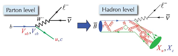
Figure 1: Parton level and hadronic level diagrams for semi-leptonic $B$ decay.

3 $B\rightarrow Dl\nu$

The decay rate for $B\rightarrow Dl\nu$ is given by

$$\frac{d\Gamma}{dw}=\frac{G_{F}^{2}}{48\pi^{3}}|V_{cb}|^{2}(m_{B}+m_{D})^{2}m_{D}^{3}(w^{2}-1)^{\frac{3}{2}}{\cal F}_{D}^{2}(w)$$ (2)

where the convention is to use

$$w=\frac{m_{B}^{2}+m_{D}^{2}-q^{2}}{2m_{B}m_{D}}=\frac{E_{D}^{*}}{m_{D}}$$ (3)

instead of $q^{2}$ and $\cal F_{D}$ is the form-factor. Because this is $0^{-}\rightarrow 0^{-}$ transition only one form-factor is needed.

In the heavy quark symmetry (HQS) limit (i.e. for infinite $c$- and $b$-quark masses) ${\cal F_{D}}(w=1)=1$. However, as quarks are not infinitely heavy, a correction is needed. Lattice QCD calculations of Hashimoto and collaborators finds ${\cal F_{D}}(w=1)=1.069\pm 0.026$ [2]. Because ${\cal F_{D}}(1)$ may change as theory matures, it is common practice to give the experimentally measured quantity ${\cal F_{D}}(1)\times|V_{cb}|$.

To extrapolate to $w=1$ (or equivalently integrate over the full $w$ range with normalization at $w=1$ imposed) the shape of ${\cal F_{D}}(w)$ is also needed. In principle this could be measured, but the rate at $w=1$ vanishes, so some theoretical input that constrains the form-factor shape has to be deployed.

The most popular (though not the first) ${\cal F_{D}}$ parameterization is that of Caprini, Lelloch and Neubert (CLN) [3] based on Heavy Quark Effective Theory (HQET) and using dispersion relations to constrain the parameterization. The CLN parametrization for ${\cal F_{D}}(w)$ is

$${\cal F}_{D}(w)={\cal F_{D}}(1)\times(1-8\rho^{2}z+(51\rho^{2}-10)z^{2}+(252\rho^{2}-84)z^{3}$$ (4)

where $z\equiv(\sqrt{w+1}-\sqrt{2})/(\sqrt{w+1}+\sqrt{2})$ is an improved expansion variable (that converges faster than $w-1$).

Some other parameterizations are provide by Boyd, Grinstein and Lebid (BGL) [4] and LeyYaonac, Oliver and Raynal (LeYor) [5].

In all these parameterizations we are left with only one parameter to fit – $\rho^{2}$ – which is the derivative of ${\cal F_{D}}(w)$ w.r.t. $w$ at $w=1$.

Figure 2: Background subtracted $w$-distribution (called ${\hat{y}}$ here) as measured by BELLE. Points are data and histograms are fits.

The $D\rightarrow Dl\nu$ analysis has been carried out by the CLEO [6] and BELLE [7] collaborations. CLEO used both ${\overline{B}}^{-}\rightarrow D^{0}l^{-}{\overline{\nu}}$ and $B^{-}\rightarrow D^{+}l^{-}{\overline{\nu}}$ modes, while BELLE only used the $B^{-}\rightarrow D^{+}l^{-}\overline{\nu}$. Figure 2 shows the background subtracted $w$-distribution obtained by BELLE (note in BELLE’s notation $w$ is called ${\hat{y}}$). The signal is extracted using the discriminating variable $cos\theta_{BY}$ defined and described in detail in section 4.

They fit by minimizing $\chi^{2}$ given by

$$\chi^{2}=\sum_{i}\left(\frac{N_{i}^{obs}-\sum_{j}\varepsilon_{ij}N_{j}(N,\rho^{2})}{\sigma_{i}}\right)^{2}$$ (5)

where $N_{j}$ is the number predicted based on Eq.(2) and $\varepsilon_{ij}$ is the efficiency for an event truly in bin $i$ to be detected in bin $j$. The errors $\sigma_{i}$ includes both the uncertainty in the observation and the uncertainty in the efficiency matrix $\varepsilon_{ij}$

The fit parameters are the number of events $N$ and the slope parameter $\rho^{2}$. The fit using the CLN parameterization (Eq.(4)) is shown as solid histogram in the figure. The dashed histogram represents the result when a simple linear parameterization is used instead of CLN. The two fits are not distinguishable.

CLEO does something similar. The results of both experiments is given table  1 along with the HFAG averages as of summer 2006.

Exp	${\cal B}(B^{-}\rightarrow D^{0}l^{-}\overline{\nu})(\%)$	$\rho^{2}$(CLN)	${\cal F}(1)\times|V_{cb}|(10^{-3})$
CLEO	$2.21\pm 0.13\pm 0.19$	$1.27\pm 0.25$	$44.8\pm 5.8\pm 3.$
BELLE	$2.13\pm 0.12\pm 0.39$	$1.12\pm 0.22$	$41.1\pm 4.4\pm 5.1$
HFAG	$2.12\pm 0.20$	$1.17\pm 0.18$	$42.4\pm 4.5$

Table 1: CLEO and BELLE results for branching fraction, $\rho^{2}$ and $|V_{cb}|$ and HFAG averages

The BELLE and CLEO results are consistent. The uncertainties are large and BELLE assigns a more conservative systematic than CLEO.

4 $B\rightarrow D^{*}l\nu$

The analysis of $B\rightarrow D^{*}l\nu$ is more complex than $Dl\nu$. There are three form-factors called $A_{1},\ A_{2}$ and $V$. To separate them an analysis in the three angles ($\theta_{l},\ \theta_{V}$ and $\chi$) and $w$ is needed. The angles are defined in Figure 3.

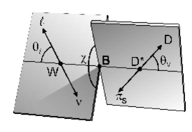
Figure 3: Definition of the angles $\theta_{l},\ \theta_{V}$ and $\chi$ that describe the decay $B\rightarrow D^{*}l\nu$.

The decay rate in terms of the four kinematic variables $w,\ \theta_{l},\ \theta_{V}$ and $\chi$ is given by

$$\frac{d\Gamma}{dw\ dcos_{l}\ dcos_{V}\ d\chi}=K|V_{cb}|^{2}q^{2}p_{D^{*}}\times$$ (6)

$$\{H_{+}^{2}(1-cos\theta_{l})^{2}sin^{2}\theta_{V}+H_{-}^{2}(1+cos\theta_{l})^{2}sin^{2}\theta_{V}+4H_{0}^{2}sin^{2}\theta_{l}cos^{2}\theta_{V}\$$

$$-2H_{+}H_{-}sin^{2}\theta_{l}sin^{2}\theta_{V}cos2\chi-4H_{0}(H_{+}\left(1-cos\theta_{l})-H_{-}(1+cos\theta_{l})\right)sin\theta_{V}cos\theta_{V}cos\chi\}$$ (7)

where $H_{\pm}$ and $H_{0}$ are helicity amplitudes related to the form-factors by

$$H_{\pm}=-(m_{B}+m_{D^{*}})A_{1}(w)\pm\frac{2p_{D^{*}}m_{B}}{m_{B}+m_{D^{*}}}V(w)$$ (8)

$$H_{0}=-\frac{m_{B}+m_{D^{*}}}{m_{D^{*}}\sqrt{q^{2}}}(m_{D^{*}}(wm_{B}-m_{D^{*}})A_{1}(w)-\frac{4m_{B}^{2}p_{D^{*}}^{2}}{(m_{B}+m_{D^{*}})^{2}})A_{2}(w).$$ (9)

In principle, by doing a spin-parity analysis in bins of $w$ the form-factors could be measured without any model dependence. In practice the statistics are inadequate and we have to resort to some parameterization.

HQET relates the three form-factors describing the decay to a single common form-factor called the Isgur-Wise function. The relationships are

$$A_{2}(w)=\frac{R_{2}(w)}{R_{*}^{2}}\frac{2}{w+1}A_{1}(w)$$ (10)

$$V(w)=\frac{R_{1}(w)}{R_{*}^{2}}\frac{2}{w+1}A_{1}(w)$$ (11)

$$A_{1}(w)=R_{*}\frac{w+1}{2}h_{A_{1}}(w)\rightarrow R_{*}\frac{w+1}{2}\xi(w)$$ (12)

where $R_{*}=2\sqrt{m_{B}m_{D*}}/(m_{B}+m_{D^{*}}).$

The CLN [3] formalism is again the most popular. They provide the $w$ dependence of $R_{1}(w)$ and $R_{2}(w)$ and a parameterization in terms of the slope $\rho^{2}$ at $w=1$ of the common form-factor $h_{A_{1}}(w)$. In fitting for the form-factors the intercepts $R_{1}(w=1),\ R_{2}(w=1)$ and $\rho^{2}$ are taken as the independent parameters.

The CLN parameterizations are

$$R_{1}(w)=1.27-0.12(w-1)+0.05(w-1)^{2},$$ (13)

$$R_{2}(w)=0.79+0.15(w-1)-0.04(w-1)^{2}$$ (14)

for the form-factor ratio parameters and

$$h_{A_{1}}(w)=h_{A_{1}}(1)(1-8\rho^{2}z+(53\rho^{2}-15)z^{2}-(231\rho^{2}-91)z^{3}$$ (15)

for the common ‘Isgure-Wise’ like form-factor.

Outside the heavy quark limit where $h_{A_{1}}(w)=\xi(w)$ and the value at $w=1$ is 1.0, $h_{A_{1}}(w=1)$ has to be taken from theory. The best estimate comes from lattice QCD [2]. It is $0.919^{+0.030}_{-0.035}$.

BABAR measures the decay rates as function of $\theta_{l},\ \theta_{V},\ \chi$ and $w$. Because of the missing neutrino these cannot be directly obtained from the measured tracks. Thus, a partial reconstruction technique, (illustrated in Figure 4), which allows a reasonable accurate approximation to be made, is used. Using the kinematic constraints expressed in Figure 4 the cosine of the angle between the $B$ direction and the direction of the lepton-$D^{*}$ system ($\mathbf{P}_{Y}=\mathbf{P}_{D*}+\mathbf{P}_{l}$) can be obtained as follows:

$$cos\theta_{BY}=\frac{2E_{B}E_{D^{*}+l}-m_{B}^{2}-m_{D^{*}+l}^{2}}{2|\mathbf{P}_{D^{*}}|\mathbf{P}_{Y}|}$$ (16)

where lepton and $D^{*}$ momenta are measured and $|\mathbf{P}_{B}|$ can be estimated from the beam energies. Note the same construction is used for $Dl\nu$ with, of course, $D\rightarrow D^{*}$

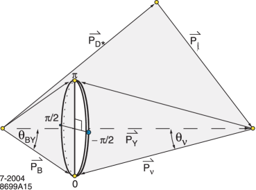
Figure 4: Kinematics of $B\rightarrow D^{*}l\nu$ that allow $cos\theta_{BY}$ to be reconstructed.

The azimuthal angle $\phi_{BY}$ of $\mathbf{P}_{B}$ around the $Y$ direction is undetermined. The kinematic variables $cos\theta_{l},\ cos\theta_{V},\ \chi$ and $w$ can be calculated for any choice of $\phi_{BY}$. Averaging over $\phi_{BY}$ gives reasonable estimators of their values. BABAR uses points at $\phi_{BY}=0,\ \pi,\ \pm\pi/2$ weighted by the $B$ production angular distribution ($\propto sin^{2}\theta_{B}$) to perform this average.

Only and CLEO [9] and BABAR [10, 11] have attempted form-factor measurements. BABAR uses two method: a likelihood fit to the full $4-d$ distribution of the kinematics variables ($w,\ \theta_{l},\ \theta_{V},\ \chi$) and a simultaneous fit to the one-dimensional $w$, $cos\theta_{l}$ and $cos\theta_{V}$ projections. CLEO also does a 4-d likelihood fit. I’ll describe the BABAR methods in some detail.

For the $4-d$ likelihood fit it’s difficult to construct the full, correlated PDF (including efficiency and resolution) for the measured variables $w,\ \theta_{l},\ \theta_{V}$ and $\chi$, so BABAR resorts to the ‘integral method’ that avoids the need to know this complicated PDF. With the integral method only the integral of the efficiency and the theoretical PDF Eq.(6) are needed.

The extended likelihood (include resolution) is given by

$$log{\cal L}=\sum_{e}log\tilde{F}(\tilde{\Omega}_{e}|\mu)-\int d\tilde{\Omega}\tilde{F}(\tilde{\Omega}|\mu)$$ (17)

where $\tilde{\Omega}$ represents measured quantities and $\tilde{F}(\tilde{\Omega}|\mu)$ represents their PDF for parameters $\mu$. The sum is over events. Using the approximation

$$\tilde{F}(\tilde{\Omega}|\mu)\approx F(\tilde{\Omega}|\mu)\times\frac{\tilde{F}(\tilde{\Omega}|\mu_{mc})}{F(\tilde{\Omega}|\mu_{mc})}$$ (18)

we obtain

$$log{\cal L}\approx\sum logF(\tilde{\Omega}_{e}|\mu)-\tilde{I}(\mu,\mu_{mc})$$ (19)

with

$$\tilde{I}(\mu,\mu_{mc})=\int{d\tilde{\Omega}F(\tilde{\Omega},\mu)\times\left(\frac{\tilde{F}(\tilde{\Omega}|\mu_{mc})}{F(\tilde{\Omega}|\mu_{mc})}\right)}$$ (20)

which can be obtained by Monte Carlo integration as

$$\tilde{I}(\mu,\mu_{mc})\approx\frac{1}{N_{mc}}\sum\frac{F(\tilde{\Omega}_{imc}|\mu)}{F(\tilde{\Omega}_{imc}|\mu_{mc})}.$$ (21)

It can be shown that for $\mu_{true}$ equal $\mu_{mc}$, the result of this approximation is unbiased. The procedure can be iterated by re-weighting to get $\mu_{mc}\approx\mu_{fit}$ which is close enough. Extra contributions to the error from MC statistics need to be evaluated, but knowledge of $4-d$ efficiency-resolution function is not required. Background is subtracted event-by-event using MC events to avoid breaking the factorization that leads to Eq.(19).

Since there is no explicit PDF $\tilde{F}$ constructed, the MC is re-weighted to fitted values of $R_{1}(1),\ R_{2}(1)$ and $\rho^{2}$ (histogram) and compared to the data (points) to see if fit is good. Figure 5 shows the four projects and Figure 6 shows the $\chi$ projection for six bins of $cos\theta_{V}$. The agreement with the fit represented by re-weight MC is excellent and reproduces even the details of the interference in the $\chi$ vs. $cos\theta_{V}$ plots.

Figure 5: Distribution of $w,\ cos\theta_{l},\ cos\theta_{V},\ \chi$ as well as lepton momentum $p_{l}$ and “slow” pion momentum $p_{t}(\pi_{s})$.

Figure 6: Distribution of $\chi$ for six cuts on $cos\theta_{V}$.

The results are

$$R_{1}(w)=1.396\pm 0.046\pm 0.027$$ (22)

$$R_{2}(w)=0.885\pm 0.046\pm 0.013$$ (23)

$$\rho^{2}=1.145\pm 0.066\pm 0.035$$ (24)

The BABAR results are consistent with the pioneering CLEO measurement of $R_{1}=1.18\pm 0.30\pm 0.12,\ R_{2}=0.71\pm 0.22\pm 0.07$. The slope parameter $\rho^{2}$ also agrees when equivalent parameterizations of $h_{A_{1}}(w)$ are used. The values are also consistent with theoretical expectations. Since, $|V_{cb}|$ is highly sensitive to $R_{1}$ and $R_{2}$, this measurement leads to substantial reduction in the error achievable on it.

The second BABAR method works with projections in $w,\ cos\theta_{l}$ and $cos\theta_{V}$. The dihedral angle $\chi$ is not used because it has little sensitivity when one integrates over the other angles. The projection method is not as statistical powerful for the form-factors as the full $4-d$ fit, however, it has the advantage that the background can be estimated and removed in a manner that is nearly independent of the MC. This allows higher multiplicity $D$-decays to be used. The $4-d$ method only used the $D\rightarrow K\pi$ in order to keep the systematic error from dependence on MC simulation of the background shape under control.

The projection method divides each variable into ten bins and fits the $cos\theta_{BY}$ distribution in each bin to obtain estimates of the signal and background in that bin. The shape of the $cos\theta_{BY}$ distribution for background and signal is taken from MC and whenever possible from data control samples, but no assumption about the shape of the background distributions in $w,\ cos\theta_{l}$ or $cos\theta_{V}$ is used. Thus the resulting projection plots are only weakly dependent on the MC simulation.

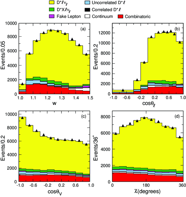
Figure 7: Projection results for $w,\ cos\theta_{l},\ cos\theta_{V}$. The angle $\chi$ was not part of the fit.

Figure 7 shows the results of simultaneous fits to the projection plots. The projection distributions are correlated since they share the same events; this correlation is taken into account in the fitting procedure. The triangles represent that data, the yellow the signal and the other colors the results of the $\cos\theta_{BY}$ fits for the background. The $\chi$ projection is not fit, but is only shown for completeness. The fits look good.

For BABAR’s final result they combine the results of the two method. The results are

$${\cal F}(1)|V_{cb}=(34.68\pm 0.32\pm 1.15)\times 10^{-3}$$ (25)

$$\rho^{2}=1.179\pm 0.048\pm 0.028$$ (26)

$$R_{1}=1.417\pm 0.061\pm 0.044$$ (27)

$$R_{2}=0.836\pm 0.037\pm 0.022$$ (28)

where errors are statistical and systematic respectively. In this case the CLN form (Eqs. 13-14) for $R_{1}(w)$ and $R_{2}(w)$ has been used.

This currently yields the best exclusive measurement of $|V_{cb}|=(37.74\pm 0.35\pm 1.24^{+1.32}_{-1.44})\times 10^{-3}$. The additional error is from the theoretical predictions of ${\cal F}(1)$.

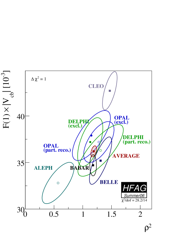
Figure 8: Summer ‘06 plot of ${\cal F}(1)|V_{cb}|$ vs. $\rho^{2}$ from HFAG.

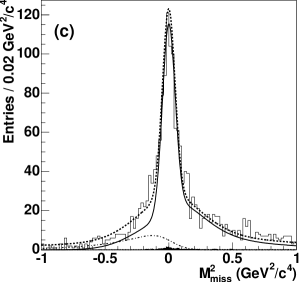
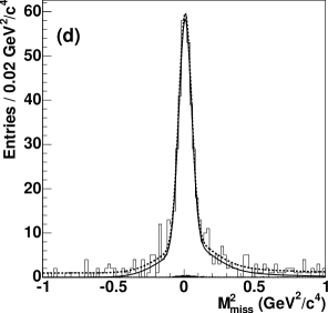
Figure 9: Missing mass against $D^{*}l\nu$ in $B^{\pm}$ recoil sample (left) and in $B^{0}$ sample (right).

HFAG has averaged the $|V_{cb}|-\rho^{2}$ results from six experiments. The summer 2006 average, which includes the BABAR improvement of $R_{1}$ and $R_{2}$ to the results of other experiments, is shown in Figure 8. The poor $\chi^{2}$ ($28/14$) is mostly due to the CLEO and ALEPH measurements. While BABAR is the single best measurement, the others make a significant contribution to the world average.

There is a persistent conflict between the $D^{*}l\nu$ branching fraction measured with charged and neutral $B$-mesons. In PDG 2006 average is $5.34\pm 0.20\%$ for neutrals and $6.5\pm 0.5\%$ for charged $B$’s. This difference would represent isospin violation, which is $\it apriori$ very unlikely. At this point it’s only $\sim 2\sigma$, so we can hope the difference will “regress-to-the-mean” as new measurements come in.

BELLE [12] has used a “recoil” technique to measure both $D^{*0}l^{+}\nu$ and $D^{*0}l\nu$ recoiling against a fully reconstructed $B^{-}$ or $\overline{B}^{0}$. While the sample is quite small, this method substantially reduces the background and thus potentially the systematic errors. BELLE has not yet fully exploited this potential as they do not give a systematic error on these branching fractions.

Figure 9 shows BELLE’s missing mass plots. The branching fractions they obtain are

$$B(\overline{B}^{0}\rightarrow D^{*}l\nu)=4.7\pm 0.24\%,\ B(B^{+}\rightarrow D^{*}l\nu)=6.06\pm 0.25\%$$ (29)

which is $\sim 4\sigma$ discrepancy, …but of course only the statistical error is taken into account. This method has the potential to shed considerable light on the issue, if the systematic uncertainties can be understood.

5 Higher mass states: $D^{**},\ D^{(*)}\pi$, etc.

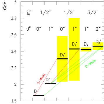
Figure 10: “…to see what he could see…and high mass charm states we might see…  [13]

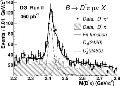
Figure 11: $D^{*}\pi$ mass distribution from $D^{0}$.

One might ask w.r.t the semi-leptonic decays to the higher mass charm states “why bother?” It seems unlikely anything very exciting will be found.

One answer might be simply “because they’re there.” In general, it’s good idea to try to understand the decay modes of particles like the $B$ as completely as possible…and you’ll never know what might be lurking there, if you don’t look…we need to see what we can see (see Figure 10).

A more practical answer is “engineering.” The so-called ${\cal D}^{**}$ states and $D^{*}n\pi$ are the dominant backgrounds to $Dl\nu$ and $D^{*}l\nu$ and the lack of understanding of these backgrounds is a major source of systematic error for $V_{cb},\ \rho^{2}$ and the form-factor ratios $R_{1}$ and $R_{2}$.

HQET also makes predictions about the form-factors of excited $D$-mesons and perhaps lattice QCD can too. Measurements in the high mass sector can test the theory that underlies the extraction of $|V_{cb}|$ and are of some interest in themselves.

What could be there? In terms of resonance, this also shown in Figure 10 where the predictions for the resonant structure based on HQET are given. There are two narrow resonances – the $D_{1}(2420)$ and the $D_{2}^{*}(2460)$ which should be relatively easy to detect and, in fact, are already seen in semi-leptonic $B$-decay. The wide $D_{0}^{*}$ and $D_{1}^{*}$ will be hard to distinguish from the non-resonant $D^{(*,**)}n\pi$ contributions.

The D0 experiment [14] has observed the narrow states in $B\rightarrow D^{*}\pi l\nu+X$. The measurement does not strictly correspond to exclusive $D^{*}\pi$ though that’s likely to be a major component of the signal. The $D^{*}\pi$ mass plot is displayed in Figure 11. The $D_{2}(2460)$ corresponds to the shoulder on the right side of the bump. Only the product production$\times$branching fraction are directly measured, they are

$$B\rightarrow\overline{D}_{1}l\nu,\ \overline{D}_{1}^{0}\rightarrow D^{*-}\pi^{+}=0.087\pm 0.007\pm 0.014,$$ (30)

$$B\rightarrow\overline{D}_{2}l\nu,\ \overline{D}_{2}^{*0}\rightarrow D^{*-}\pi^{+}=0.035\pm 0.007\pm 0.008,$$ (31)

$$ratio\ \overline{D}_{2}^{*0}/\overline{D}_{1}^{0}=0.39\pm 0.09\pm 0.12.$$ (32)

Using $b\rightarrow B^{-}=0.39\pm 0.09\pm 0.12$ and isospin symmetry, the absolute branching fractions can be estimated as $0.33\pm 0.06\%$ for the $D_{1}$ and $0.44\pm 0.16\%$ for the $D_{2}^{*}$.

The OPAL [15] collaboration does a similar measurement, but is unable to see the $D_{2}$. They get

$${\cal B}(b\rightarrow\overline{B})\times{\cal B}(D_{1}^{0}l^{-}\overline{\nu})\times{\cal B}(D^{*+}\pi^{-})=(2.64\pm 0.79\pm 0.39)\times 10^{-3}.$$ (33)

For the $D_{2}$ they get $(0.26\pm 0.59\pm 0.35)\times 10^{-3}$ which is consistent with zero.

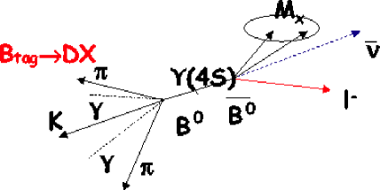
Figure 12: Illustration of reconstruction missing mass $M_{miss}$ in the system recoiling against a fully reconstructed $B$ and some hadrons (represented by $M_{X}$). For the exclusive channels of interest $M_{X}$ is composed of $D^{(*)}\pi$ and $M_{miss}=M_{\nu}=0$ for signal.

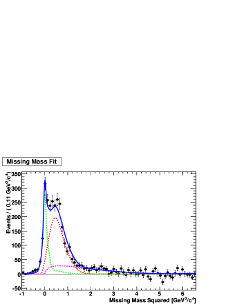
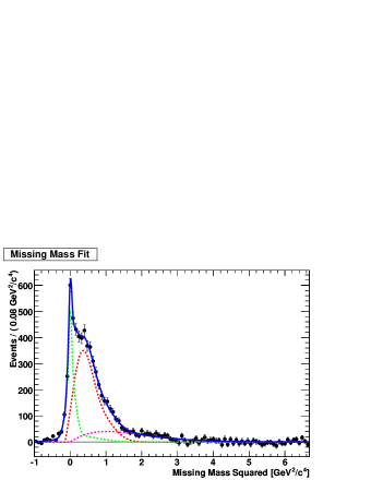
Figure 13: Missing mass against $Dl$ in full recoil tagged events. Left is $B^{0}$ decays and right charged $B$ decays.

BABAR [16] also makes a measurement of the higher mass states using an inclusive method that also yields estimate of $Dl\nu$ and $D^{*}l\nu$. This is done looking at the semi-leptonic decays recoiling against a fully reconstructed $B$.

Using a recoil tagged sample, the distributions of the missing mass against $Dl$, shown in Figure 13, can be constructed. The decay modes $Dl\nu,\ D^{*}l\nu$ and the modes $D^{(}*)n\pi$ have different shapes in missing mass, so the missing mass distribution can be used to disentangle them. Roughly speaking, $Dl\nu$ is peaked at zero, $D^{*}l\nu$ peaks a bit higher ($\sim 0.8GeV$) and the rest is broad.

While missing mass is the most powerful variable for discriminating these decay contributions, there is also discriminating power in the lepton momentum ($p_{l}$) spectrum and in the number of extra tracks not used reconstructing the $Dl$. BABAR extracts the relative branching fractions of these three components by fitting simultaneously to the missing mass, $p_{l}$ and extra-track distributions using PDFs determined by the data and validated with the Monte Carlo. The results are normalized to the semi-leptonic decay rate ($B\rightarrow DXl\nu$). Small contributions from baryons in the final state are missing.

The results are summarized in Table 2. If I use semi-leptonic branching fractions from the 2006 PDG (neglecting small non-$DXl\nu$ contributions) to estimate absolute branching fractions for $D^{*}l\nu$, I get $6.34\pm 0.2\%$ for charged $B$’s and $5.58\pm 0.32\%$ for the neutrals. I’ve only kept the statistical errors. Under the assumption that most systematics are common, this is again a $\sim 2\sigma$ descrepency…however not all the systematics are common so the discrepancy may not really be that large.

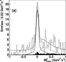
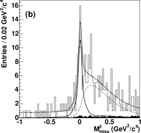
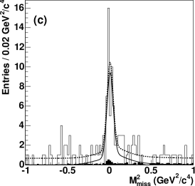
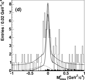
Figure 14: Missing mass against $D^{*}\pi$ in full recoil tagged events. The modes considered are (a) $D^{+}\pi^{-}l^{-}\overline{\nu}$, (b) $D^{0}\pi^{+}l^{-}\overline{\nu}$, (c) $D^{*+}\pi^{-}l^{-}\overline{\nu}$ and (d) $D^{*0}\pi l^{-}\overline{\nu}$.

The BELLE paper [12] also contains results on the higher mass states $D\pi l\nu$ and $D^{*}\pi l\nu$. In fact, these are the main results of their paper and the $D^{*}l\nu$ decays are not the focus of the analysis. This technique also employs recoil tagged sample (see Figure 12 again), but looks at the missing mass recoiling against the specific states. Figure 14 show the missing mass distribution obtained for the four $D^{(*)}\pi$ modes reconstructed. The signal in these plots appears at zero. There is little background in the $D^{*}\pi$ modes and even in the $D\pi$ modes the signals are evident.

The branching fractions obtained are

$$B(D^{+}\pi^{-}l^{-}\overline{\nu})=0.54\pm 0.07\pm 0.07\pm 0.06\%,$$ (34)

$$B(D^{0}\pi^{+}l^{-}\overline{\nu})=0.33\pm 0.06\pm 0.06\pm 0.03\%,$$ (35)

$$B(D^{*+}\pi^{-}l^{-}\overline{\nu})=0.67\pm 0.11\pm 0.09\pm 0.03\%,$$ (36)

$$B(D^{*0}\pi^{+}l^{-}\overline{\nu})=0.65\pm 0.12\pm 0.08\pm 0.05\%,$$ (37)

where in addition to the usual systematic uncertainties there is an additional contribution from using the $Dl\nu$ and $D^{*}l\nu$ to normalize the results. The higher mass contribution to the total branching fraction should be $\sim 10.4-2.1-5.3=3\%$. BELLE’s observed $D^{*}\pi$ contribution to $B^{0}$ decays is $\approx(0.98\pm 0.13\%)$ which accounts for only $\sim 1/3$. If we assume the total isospin of the $D\pi$ system is $1/2$ then there should be $1/2$ as many again in the unobserved charge $D$ with $\pi^{0}$ modes for a total, of $1.5\pm 0.2$ thus accounting for $\sim 1/2$ of the missing modes. The same argument applies to the charged $B$, where the estimate $D\pi$ branching fraction corrected for isospin is $1.8\pm 0.20$. So it seems, like there must be some contribution from states with two pions. Both of these are consistent with BABAR’s estimate using the $Dl$ missing mass.

Using isospin to relate $B^{0}$ and $B^{+}$ modes we could average to produce a somewhat more accurate estimate. However, considering the unsettled state of $D^{*}l\nu$ branching fractions, it’s probably best to just settle for the statement that $D^{(*)}\pi$ can account for $\sim 1/2$ the decays with hadronic masses $m_{had}>m_{D^{*}}$.

Another interesting number is the ratio $R=D\pi/D^{*}\pi$. To estimate this I average the BELLE’s numbers for $B^{0}$ and $B^{+}$ and assume systematics cancel in the ratio. I find $R=1.58\pm 0.26$ (stat error only).

Using D0’s estimate of the branching fraction to the narrow state $D_{1}^{0}$ (see above), I find that $\sim 35\%$ of $D^{*}\pi$ are from this narrow state. This suggest that some narrow states might be visible in BELLE’s recoil samples.

These are very beautiful measurements. Given that there’s still a percent of so in other modes it would be interesting to measure modes like $D^{*}\pi\pi$.

Ratio	$B^{-}(\%)$	$B^{0}(\%)$
$Dl\nu$	$22.7\pm 1.4\pm 1.5$	$21.5\pm 1.6\pm 1.3$
$D^{*}l\nu$	$58.2\pm 1.8\pm 3.0$	$53.7\pm 3.1\pm 3.6$
$D^{*,**}n\pi l\nu$	$19.1\pm 1.3\pm 1.9$	$24.8\pm 3.2\pm 3.0$

Table 2: Ratios of $Dl\nu,\ D^{*}l\nu$ and $D^{*,**}n\pi$ to $DXl\nu$ for charged and neutral $B$-mesons.

6 What to do?

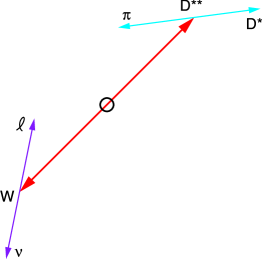
Figure 15: Possible fake $D^{*}l\nu$ from a $D^{**}l\nu$ decay – a neutrino goes “forward” and $\pi$ goes “backward” the missing mass gets small and the event mimics $D^{*}l\nu$. Any decay with $\nu$ and $\pi$ moving the same direction will produce a successful $cos\theta_{B}Y$ construction with just a slightly higher neutrino momentum. The number of $D^{**}$ decays near this configuration will be influenced by the $D^{**}$ form-factors.

• We need to resolve the discrepancy between $D^{*}l\nu$ measured in $B^{0}$ and $B^{+}$ decays!

  • Isospin violation is most unlikely

  • It’s only $\sim 2\sigma$, so may be we’re just chasing a fluctuation

  • Could there be high-spin, high-mass states that can mimic $D^{*0}l\nu$ modes?

    • Try to get solid theory predictions for spin 2 states implemented in MC and seek parameters that might cause such a problem, i.e., investigate the theoretical constraints on the high mass states.

    • Example of “$D^{**}$” faking $D^{*}l\nu$ is shown in Figure 15

  • Maybe slow pions from $D^{*}\rightarrow D\pi$ decays not well understood?

    • This is not a likely explanation as there aren’t many events produced at low $w$ (high $q^{2}$) so they should not affect branching fraction too much

    • Try using $D^{+}\pi^{0}$ decay instead of $D^{0}\pi^{+}$ to see if the same answer is obtained with a different slow $\pi$ efficiency

    • Repeat BELLE style missing mass analysis for $D^{*}l\nu$ with careful attention to systematics and background. Hopefully many systematics would cancel in the charge to neutral $B$ ratios

• $D\pi l\nu$ accounts for about half the missing modes. What is the rest?

  • Measure $D^{*}\pi\pi$. Is this possible with current statistics?

  • Wide states are hard. They need a full spin-parity analysis to extract phase shifts – an analysis that is not feasible with the current generation of $B$ factories

• Test HQET. Needs higher precision form-factor measurements and ultimately model independent measurements

7 Summary

We already know quite a bit. The HFAG world average is ${\cal F}(1)_{cb}$ is $36.2\pm 0.6\times 10^{-3}$. The form-factor parameters $R_{1}$ and $R_{2}$ have been measured to be $1.42\pm 0.07$ and $0.84\pm 0.043$, respectively. Two narrow contributions to the high mass region are known at the $10-20\%$ level. It’s been established that $D\pi$ (resonant+wide+nonresonant) can account of $\sim 1/2$ of the branching fraction to higher mass states.

The biggest outstanding problem is tensione between the $D^{*}l\nu$ decay in $B^{0}$ ($\sim 5\%$) and $B^{+}$ decay ($\sim 6\%$). However, it’s only $\sim 2\sigma$, so it probably will resolve itself in due course – which is not to say we shouldn’t look for a systematic problem in the meanwhile.

While $R_{1}-R_{2}$ are well enough measured for current $|V_{cb}|$ measurements given the other errors and the theory errors. Improved measurements could probe the HQET based theoretical assumptions.

References

- [1] M.R. Ahmady et al, KEK Theory Group, hep-ph/0109061.
- [2] Hashimoto et al., Phys. Rev. D66 (2002) 01450 [hep-lat/9810056].
- [3] I. Caprini, L. Lellouch and M. Neubert, Nucl. Phys. B 530, 153 (1998) [hep-ph/9712417].
- [4] C. G. Boyd, B. Grinstein and R. F. Lebed, Nucl. Phys. B 461, 493 (1996) [hep-ph/9508211].
- [5] A. Le Yaouanc, L. Oliver and J. C. Raynal, Phys. Rev. D 67, 114009 (2003) [hep-ph/0210233].
- [6] CLEO, Phys. Rev. Lett.82:3746,1999, CLNS 98/1594 hep-ex/9902005
- [7] BELLE, Phys.Lett. B526 (2002) 258-268, [hep-ex/0111082]
- [8] N. Isgur and M. B. Wise, “Weak transition form-factors between heavy mesons,” Phys. Lett. B 237, 527 (1990).
- [9] J.E. Duboscq et.al. (CLEO Collaboration), Phys. Rev. Lett. 76, 3898 (1996).
- [10] B. Aubert et.al. (BABAR Collaboration), Phys. Rev. D74, 092004 (2006).
- [11] B. Aubert et.al. (BABAR Collaboration), ICHEP 2006, hep-ph/0607076
- [12] D. Liventsev et al., Phys. Rev. D 72, 051109 (2005).
- [13] American folk/children’s song “The bear went over the mountain” – traditional – sung in the backseat until the adults go insane!
- [14] V. M. Abazov et al. (D0 Collaboration), Phys. Rev. Lett. 95, 171803 (2005), hep-ex/0507046.
- [15] G. Abbiendi et al. (OPAL Collaboration), Eur. Phys. J. C 30, 467 (2003), hep-ex/0301018.
- [16] “Measurement of the Relative Branching Fractions of Decays in Events with a Fully Reconstructed Meson,” hep-ex/0703027, submitted to PRD-RC.
- [17] L. da Ponte, Trans. N. Y. Acad. Sci., 3, 27 (1795).