Dpto. de Física Teórica y del Cosmos & CAFPE
Universidad de Granada
Study Of Accelerator Neutrino Interactions in a Liquid Argon TPC
Memoria presentada por
Alberto Martínez de la Ossa Romero.
Directores:
Dr. Francisco del Águila Giménez y
Dr. Antonio Bueno Villar.
- Enero de 2007 -
D. Francisco del Águila Giménez, Catedrático de Universidad, y D. Antonio Bueno Villar, Profesor Titular de Universidad,
CERTIFICAN: que la presente memoria, Study Of Accelerator Neutrino Interactions In A Liquid Argon TPC, ha sido realizada por D. Alberto Martínez de la Ossa Romero bajo su dirección en el Dpto. de Física Teórica y del Cosmos, así como que éste ha disfrutado de estancias en el extranjero por un periodo superior a tres meses, tanto en el CERN (Suiza) como en el Instituto Superior Técnico de Lisboa (Portugal).
Granada, 24 de Enero de 2005
Fdo: Francisco del Águila Giménez Antonio Bueno Villar
Introduction
In the thirties, W. Pauli put forward the idea of a new neutral particle that appeared together with the electron in the final state of nuclear beta decay. In its origin, this was “a desperate solution” to preserve the idea of energy conservation in physical processes. Apparently energy disappeared in beta decay reactions without leaving any trace. In fact, that was the case since energy was carried away by the invisible neutrino. More than twenty years elapsed, till C. Cowan and F. Reines observed for the first time electron antineutrinos coming from a nuclear reactor. Despite the multiple applications neutrinos had in Particle Physics through these years, we still know very little about these elusive particles. Almost a decade ago, we had strong experimental evidence that atmospheric neutrinos do oscillate (they change their leptonic flavour) in their path to the detector. A similar mechanism is at the heart of the so-known solar neutrino problem. This set of results was beautifully confirmed through experiments done with man-made neutrinos (those coming from reactors and accelerators). We are now convinced that neutrinos are massive particles, however with oscillation experiments, we cannot tell anything about absolute neutrino masses. There are other experiments that carefully measure the kinematics of reactions were neutrinos are involved (like the tritium beta decay) that are able to restrict the absolute mass of the electron neutrino below 2 eV. Although massive, neutrinos have a very tiny mass compared to their corresponding charged leptons.
The evidence for neutrino masses gave rise to a true revolution in Particle Physics, since this was the first solid clue about the existence of new Physics beyond the Standard Model. Within this model, the neutrino was exclusively left-handed and therefore could not be given a Dirac mass term. Experimentally we have never observed right-handed neutrinos, but there is no fundamental principle that forbids those neutrino states. In fact, many extensions of the Standard Model do contemplate their existence.
After a brief introduction of the Standard Model in Chapter 1, we will see how to build mass terms for neutrinos. We will deal with fundamental questions like the Dirac or Majorana nature of neutrinos, the hierarchy problem, the see-saw mechanism or with the possible existence of heavy neutrinos at the TeV scale. With rather generality, we introduce the neutrino mixing matrix that allows us to describe the results obtained in neutrino oscillation experiments. Since many theoretical models propose the existence of heavy neutrinos, weakly mixed with the light ones, we perform a phenomenological study in Sec. 1.4 on the precision that next-generation lepton colliders will have in establishing limits to such an admixture and on the heavy neutrino masses. This work is thoroughly described in Ref. [1].
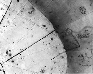
The rest of the thesis is devoted to assess the potentialities of Liquid Argon (LAr) TPCs for the study of neutrino properties. Nowadays there is a tremendous experimental effort going on in order to precisely measure the mixing angles, neutrino masses and the existence of a possible CP violation in the leptonic sector. In this context, LAr TPCs will allow us to study neutrino interactions with matter with unprecedented precisions, since the detector is fully sensitive and acts as a fine-grained track detector, recording very precisely the deposited energies of particles that propagate through argon, making thus possible an accurate reconstruction of a large variety of events. Moreover, this device records events with an imaging quality similar to those of ancient bubble chambers (see Fig. 1), but with the additional advantage of providing fully-automatized three dimensional reconstruction of the events.
 |
 |
The LAr TPC technology is discussed in Chapter 2, where we discuss all the relevant technical details. One of the major challenges we faced during this work was the development of a set of tools and procedures that allowed us to perform a three dimensional and calorimetric reconstruction of the recorded neutrino interactions. The goal was to exploit the detector capabilities in order to obtain an extremely accurate reconstruction of the neutrino event kinematics. To this purpose, we have worked with a small LAr TPC prototype having an active volume of 50 liters (see Chapter 3 for further details). In Chapter 4 we discuss the reconstruction tools. Thanks to them, in Chapter 5 we have carried out a careful study of quasi-elastic muon neutrino interactions recorded in our detector. Those multi-GeV neutrinos were produced in the CERN WANF neutrino facility. Despite the small size of our prototype, we have carried out a full study of the quasi-elastic reactions. Those reactions were extensively studied during the sixties and the seventies in experiments with bubble chambers, however we still lack a precise modeling of the behavior of nuclear matter after a neutrino interacts with it. A systematic study of neutrino interactions with LAr TPCs will allow to improve sensibly the Monte-Carlo simulations of nuclear effects. The study of quasi-elastic interactions, published in Ref. [2], has been completed with the measurement of the charged-current quasi-elastic total cross section for multi-GeV neutrinos. This measurement, together with a careful evaluation of the associated systematic errors is described in Sec. 5.4 and has given rise to the article described in Ref. [3].
The thesis also includes, in Chapter 6, a study of the capabilities a LAr TPC would have when searching for direct appearance in oscillations by means of kinematical criteria. We carefully analyze the performance of several statistical techniques for pattern recognition, applied to look for very few events in a beam mostly composed of . The study has been published in Ref. [4].
Introducción
Corrían los años 30 cuando por vez primera W. Pauli propuso la existencia de una nueva partícula neutra que acompañaba al electrón en los procesos de desintegración beta. En su origen, esto no fue más que una “solución desesperada” por salvaguardar el sagrado principio de la conservación de la energía: parecía ser entonces que en determinados procesos de desintegración nuclear la energía desaparecía, se esfumaba sin dejar rastro. Efectivamente así ocurría, se la llevaba el invisible neutrino. Así las cosas, todavía tuvieron que pasar más de 20 años hasta que C. Cowan y F. Reines consiguieran observar por primera vez neutrinos procedentes de un reactor nuclear. A pesar del tiempo transcurrido desde su descubrimiento, hoy en día los neutrinos continuan siendo un misterio. Hace aproximadamente una década se produjo la confirmación experimental de que los neutrinos procedentes del sol y la atmósfera terrestre oscilan o cambian de sabor leptónico en el transcurso de su camino hacia el detector. En los años sucesivos, la existencia de estas oscilaciones pudo ser corroborada por experimentos de última generación realizados con neutrinos producidos artificialmente en reactores y aceleradores. Aunque los experimentos de oscilaciones implican necesariamente que deben existir distintos estados de neutrino cuya diferencia de masas sea finita, nada dicen acerca del valor absoluto de las mismas. Existen, sin embargo, otros experimentos basados en el estudio cinemático de reacciones de neutrinos (como la desintegración beta del tritio) que restringen la escala de masas por debajo de 2 eV. La conclusión de estos resultados experimentales es clara: Los neutrinos tienen, aunque muy pequeña, una masa no nula.
El descubrimiento de que los neutrinos son masivos supuso una auténtica revolución en la Física de Partículas, ya que representaba la primera evidencia sólida acerca de la existencia de nueva Física más allá del Modelo Estándar. En él, el neutrino es una partícula sin las componentes quirales diestras necesarias para dotar de masa a cualquier fermión de Dirac. Esto último se infiere del hecho de que, dentro de los límites de error experimentales, nunca se han observardo neutrinos con helicidad positiva, aunque en realidad no existe ningún principio físico fundamental que lo prohíba. De hecho, existen numerosas hipótesis que dan lugar a modelos teóricos que extienden el Modelo Estándar e incorporan la posibilidad de tener neutrinos con masas distintas de cero.
Tras un breve repaso del Modelo Estándar, en el Capítulo 1 veremos cómo se pueden construir términos de masa para los neutrinos. Cuestiones como el carácter de Dirac o de Majorana de los neutrinos, el problema de las jerarquías y el mecanismo del balancín, o la posible existencia de neutrinos pesados a la escala del TeV, son tratadas en este Capítulo. De una forma efectiva y completamente general introducimos la matriz de mezcla de los neutrinos, que en el marco del Modelo Estándar minimal con neutrinos masivos y conjuntamente con las masas de éstos, permite describir los fenómenos de oscilaciones de neutrinos. Puesto que muchos de los modelos teóricos proponen en sus soluciones la existencia de neutrinos pesados, débilmente mezclados con los lígeros, en la Sección 1.4, realizamos un estudio fenomenológico sobre la precisión con la que los colisonadores de leptones de próxima generación podrán establecer los límites de esa mezcla y de las masas de los neutrinos pesados. Este trabajo se detalla en la publicación de la Ref. [1].
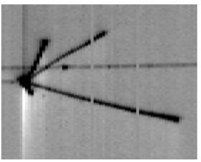
El resto de la tesis está dedicado a mostrar el potencial que poseen las cámaras de proyección temporal (TPC) de Argón Líquido (LAr) para el estudio de las propiedades de los neutrinos. Hoy en dia se está realizando un enorme esfuerzo experimental para determinar con precisión las masas de los neutrinos, sus ángulos de mezcla y una posible violación de CP en el sistema leptónico. En este contexto, las TPCs de Argón Líquido van a permitir estudiar las interacciones de los neutrinos con la materia con precisiones nunca antes alcanzadas. Todo el volumen sensible de este dispositivo actúa como un detector de trazas y de energía depositada con una alta precisión y granularidad, haciendo así posible una precisa reconstrucción cinemática de una gran variedad de sucesos. Además, su dispositivo de lectura es capaz de registrar los sucesos en distintas orientaciones con una calidad de visualización similar a la de las antiguas cámaras de burbujas (ver Fig. 2), pero con la ventaja adicional de hacer posible una reconstrucción tridimensional.
 |
 |
La tecnología del Argón Líquido se presenta en el Capítulo 2, donde se exponen los principios de la técnica de detección, las capacidades de visualización y algunas consideraciones técnicas de interés. Uno de los mayores retos de nuestra investigación consistía en el desarrollo de un conjunto de herramientas y procedimientos que hicieran posible la reconstrucción calorimétrica y tridimensional de los sucesos ionizantes que se producen en el detector. El objetivo, explotar las capacidades del detector para lograr una medida sin precedentes de la cinemática de las interacciones de neutrinos. Para tal efecto, se ha trabajado a fondo con un pequeño prototipo de Argon Líquido con unos 50 litros de volumen activo, descrito en detalle en el Capítulo 3. El Capítulo 4 está dedicado a la descripición de las herramientas de reconstrucción, así como a la discusión de su rendimiento y posibilidades. Gracias a los progresos obtenidos en los algoritmos de reconstrucción, en el Capítulo 5 hemos realizado un estudio de las interacciones quasi-elásticas de neutrinos del muón, procedentes de un acelerador de partículas a energías de varias decenas de GeV, registradas en el interior de la TPC de 50 litros. Pese a su limitado tamaño, el conjunto de sucesos recogidos ha permitido un análisis completo de la cinemática de las interacciones quasi-elasticas del tipo . Aunque este tipo de reacciones fueron extensamente estudiadas en los experimentos con cámaras de burbujas en los años 60 y 70, todavía no existe una modelización precisa de los mecanismos de interacción del neutrino con la materia nuclear. El estudio sistemático de las interacciones de neutrinos mediante los detectores de Argón Líquido permitiría una mejora substancial de las simulaciones Monte-Carlo, que tan importantes son siempre en la experimentación con neutrinos. Este trabajo, publicado en la Ref. [2], ha sido completado posteriormente con la medida de la sección eficaz de colisión quasi-elástica, vía corrientes cargadas, para neutrinos multi-GeV dispersados por núcleos de Argón. Dicha medición, junto con la evaluación de sus errores sistemáticos está expuesta en la Sección 5.4 de esta Tesis, y puede consultarse en la Ref. [3].
La memoria de la Tesis concluye en el Capítulo 6, dedicado al estudio de las capacidades que una cámara de Argón Líquido tendría a la hora de realizar una búsqueda directa de la oscilación – mediante criterios cinemáticos. Allí también analizamos el rendimiento de distintas técnicas estadísticas para el reconocimiento de señales, aplicadas al problema de búsqueda de en un haz compuesto mayoritariamente de . Toda la discusión al respecto se encuentra publicada en la Ref. [4].
Chapter 1 Neutrino interactions
The main goal of this Thesis is to prove the optimal behaviour of Liquid Argon for detection of light neutrinos, with the aim of studying neutrino oscillations. Let us then first in this Section briefly review what we know about massive neutrinos. Thus, after introducing the Standard Model (SM) of Particle Physics, we revise the two types, Dirac and Majorana, of neutrino masses and the see-saw mechanism for three generations. Then, we derive the oscillation probabilities for flavor transitions between light neutrinos, and discuss the limits on the mixing between light and heavy neutrinos.
1.1 Overview of the Standard Model
Our present understanding of the elementary particles and their interactions is described by the so called Standard Model [5, 6, 7, 8]. It contains:
-
•
Fermions with spin , which are the particles of which matter is made.
-
•
Gauge Bosons with spin 1, which act as mediators of the different interactions.
-
•
Scalars with spin 0, which are responsible of the spontaneous breaking of the electroweak symmetry.
The fermions are either leptons which are not affected by the strong interactions or quarks which are the fundamental constituents of hadrons, the particles interacting via the strong force. Leptons and quarks can be grouped into three generations according to their masses as shown in Tab. 1.1. Ordinary matter consists of fermions of the first generation. The higher mass fermions of the second and third generation are produced by particle accelerators and cosmic rays at higher energies. For every fermion there is an associated anti-fermion with the same mass but opposite additive quantum numbers.
| Quarks | |||
|---|---|---|---|
| Generation | Flavour | Charge (e) | Mass (MeV/) |
| 1st | |||
| 2nd | |||
| 3rd | |||
| Leptons | |||
| Generation | Flavour | Charge (e) | Mass (MeV/) |
| 1st | |||
| 2nd | |||
| 3rd | |||
| Interaction | Gauge | Relative | Range (m) | Participating |
| boson(s) | strength | fermions | ||
| strong | gluons () | quarks | ||
| electromagnetic | photons () | all charged | ||
| weak | , | all | ||
| gravitational | [graviton (G)] | all |
Fermions interact with each other via the exchange of the gauge bosons listed in Tab. 1.2. The photon is the gauge boson which mediates the electromagnetic interactions and couples to all charged particles. All fermions interact weakly exchanging the massive gauge bosons and . The strong interaction acts only on quarks and is carried by gluons. To complete the list of the known forces, gravity has to be mentioned. It affects all particles and is assumed to be carried by the graviton, a spin-2 boson. However, since the effects of gravity are negligible when considering the interactions of elementary particles, it will not be further discussed.
The interactions of the Standard Model are based on the principle of local gauge invariance, which demands the Lagrangian of the theory to be invariant under transformations of the gauge group
| (1.1) |
QCD is governed by the symmetry group and the electroweak theory by . Every fermion in the SM belongs to a representation of the gauge group which uniquely determines its dynamics. The different representations where the fermions lay are summarized in Tab. 1.3. The non-Abelian character of and leads to self-interactions between the gauge bosons. In the case of QCD, this self-interaction accounts for the fact that quarks are confined into hadrons, i. e., they cannot be observed as individual particles. However, probed at higher energies they begin to behave as free particles, a property referred to as asymptotic freedom.
| Field (particle) | |||||
|---|---|---|---|---|---|
| /16 | |||||
| /23 | |||||
Whereas the gauge bosons of the electromagnetic and the strong interaction are massless, the theory of the weak interactions must also accommodate the massive and gauge boons. In order to achieve this, while retaining the gauge invariant structure of the theory, the Higgs mechanism was introduced. This, however, requires at least one additional physical particle, the Higgs boson, yet to be found.
Although the SM is a mathematically consistent, renormalizable field theory, it cannot be the final answer [11]. Even if the recently discovered neutrino masses were incorporated, more fundamental shortcomings can be noted. For example, the minimal version of the model has more than 20 parameters, which, as most physicists believe, are too many for a fundamental theory. Although incorporated in the SM, there is no explanation for the fundamental fact of charge quantization or for the CP (charge-conjugation and parity) violating interactions. There is no profound compelling for the existence of the heavier fermion generations either. Moreover, there is no prediction of the charged fermion masses which vary by more than five orders of magnitude. As accelerators reach higher energies and results become more precise answers for some of the current questions will be certainly found.
Further details on the structure of the electroweak interactions can be found in Appendix A.
1.2 Massive neutrinos
Neutrinos introduce a hierarchy problem: why are they so much lighter than their charged partners? In the SM this hierarchy is made natural making the neutrino massless. Recent experimental results strongly indicate the existence of oscillations for neutrinos produced in the atmosphere [12, 13, 14] and those coming from the sun [15, 16, 17], which can be interpreted introducing finite, non-degenerate neutrino masses. The possibility of considering neutrinos as massive particles allows for new phenomena such as the already mentioned flavor mixing and oscillations, but also magnetic moments and decays, with very important consequences in astrophysics, cosmology and particle physics. Moreover, since most extensions of the SM predict the existence of massive neutrinos, this should be considered as a potentially rich field to look for physics beyond the SM.
In this section we briefly review the formulation of neutrino masses, extending the minimal SM [18, 19, 20, 21].
Dirac mass
If as the other SM fermions neutrinos have right-handed counterparts in singlets, the standard Higgs mechanism can generate the corresponding Dirac mass term
| (1.2) |
where we assume for simplicity only one family to start with. In terms of the chiral fields (left-handed neutrino) and (right-handed neutrino)
| (1.3) |
mixing fields of opposite chirality. where is a dimensionless Yukawa coupling and is the vacuum expectation value of the Higgs field. This mass term is invariant under the global transformation , which implies the conservation of a global quantum number, in this case the lepton number .
All experiments to date are consistent with the neutrino being left-handed and the anti-neutrino being right-handed. Whether the two other states exist in Nature is at present unknown. They would not take part in the weak interactions and for this reason are named sterile. The main theoretical problem associated with this mechanism is the smallness of the neutrino mass compared to the mass of the charged leptons. Since particle masses are directly determined by the particle couplings to the Higgs field, this implies couplings differing by several orders of magnitude for particles in the same generation. The relation between lepton masses of different generations may be thought of as being “accidental”, but a large mass difference between particles belonging to the same doublet is more difficult to argue. However, light neutrinos can have also masses in the absence of their right-handed counterparts.
Majorana mass
In 1937 Majorana [22] discovered that a massive neutral fermion as a neutrino can be described by a spinor with only two independent components, imposing the so-called Majorana condition
| (1.4) |
where is the operation of charge conjugation, and the charge-conjugation matrix (see [19]). The Majorana condition (1.4) can be conveniently expressed in terms of its left-handed and right-handed components
| (1.5) |
Thus, the right-handed component of the Majorana neutrino field is not independent but obtained from the left-handed component through charge conjugation111We assume the notation , which is a right-handed field, contrary to , which is a left-handed field., and the Majorana field can be written
| (1.6) |
Using the constraint (1.5) in the mass term (1.3), we obtain the Majorana mass term
| (1.7) |
where we have inserted the factor to properly normalized the kinetic term in the Lagrangian. Hence, a mass term for purely left-handed particles (and right-handed anti-particles) can be constructed (1.7). Thus, in contrast to the Dirac case a neutrino mass term is possible even without additional (unobserved) right-handed neutrinos. It requires just one helicity state of the particle and the opposite helicity state of the anti-particle.
The Majorana mass term is not invariant under global transformations. Indeed, a lepton number violation of is produced when considering a Majorana mass term. In fact, a renormalizable theory which includes a Majorana mass term for can not be constructed using the Higgs sector of the SM. In general, a Majorana mass for the neutrino would be interpreted as a hint for new physics at higher energies, whereas a Dirac mass could be accommodated adding to the SM the right-handed neutrino states but requiring very small neutrino Yukawa couplings.
General mass terms and the see-saw mechanism
The same reasoning as for can be applied to a hypothetical (in principle) and independent right-handed Majorana neutrino, which can be equivalently written 222Right-handed sterile neutrinos will be denoted by in what follows, and by when discussing collider limits. with a mass term
| (1.8) |
The right-handed Majorana neutrino does not need to be the “partner” of the (ordinary) left-handed neutrino, but could be, instead, an independent heavier state. In general, if both exist and are independent, in addition to the Dirac mass term (1.3) also the Majorana mass terms for and , in (1.7) and (1.8) respectively, are allowed. Then, the general mass term
| (1.9) |
can be written as
| (1.10) |
It is clear that the chiral fields and do not have a definite mass, since they are coupled by the Dirac mass term. In order to find the fields with definite masses, it is necessary to diagonalize the mass matrix in Eq. (1.10). This is done by a unitary transformation
| (1.11) |
with , , real and positive and the unitary mixing matrix relating the and fields with the mass eigenstates and . This diagonalization leads to the following mixing matrix and eigenvalues
| (1.12) |
The corresponding mass eigenstates are given by
| (1.13) |
An important fact to note is that the diagonalized mass term
| (1.14) |
is a sum of Majorana masses for the Majorana fields
| (1.15) |
There are two interesting physical limits. In the first case, . Then, and become almost degenerate with a mass and mixing angle . Thus, the two Majorana eigenstates form a pseudo-Dirac neutrino state, and the associated mass term in the Lagrangian conserves lepton number to a good approximation. and are the active and sterile components (in the SM), respectively, and are maximally mixed. However, as we have already mentioned (Sec.1.2), this solution does not explain why neutrino masses are so small.
The other more interesting case is the see-saw limit [23], obtained for , in which case the masses for and are
| (1.16) |
differing enormously from each other. If , increases with decreasing for a fixed value of . Furthermore, the mixing angle approaches zero, so that and are completely decoupled. Usually, is assumed to be of the order of the quark and charged lepton masses, and is a large mass of the order of some unification scale beyond the SM. This forces the mass of the ordinary neutrino to be small, and postulates a very heavy right-handed neutrino, therefore decoupled from low energy physics. This see-saw mechanism is by far the most attractive explanation of the smallness of the ordinary neutrino masses.
1.2.1 Neutrino mixing
The hypothesis of neutrino mixing was first proposed by B. Pontecorvo for the transitions [24], in analogy with . After the discovery of the muon neutrino [25], neutrino mixing between different neutrino flavors was introduced [26]. This phenomenon appears because the neutrino flavor eigenstates , , which take part in weak interactions, are generally quantum-mechanical superpositions of different neutrino mass eigenstates (see Sec. A.1), which describe the propagation of neutrinos in space-time.
From a large variety of experimental data (see [11]), it is well known that there are just three neutrinos that participate in the weak interactions. Hence, let us consider three left-handed chiral fields , , that describe the three active flavor neutrinos and three corresponding right-handed chiral fields , , that describe three sterile neutrinos 333Let us remark, however, that the number of sterile neutrinos is not constrained by terrestrial experimental data, because they cannot be detected, and could well be different from three., which are blind to weak interactions. The corresponding mass term is given by Eq. (1.10) with
| (1.17) |
where , and are matrices and
| (1.18) |
The matrix can be diagonalized by a unitary matrix , analogous to the one in Eq. (1.12). The mass term is then written as
| (1.19) |
which is a sum of Majorana mass terms for the Majorana neutrino fields. The mixing relations between mass and weak interaction eigenstates read
| (1.20) |
This mass term allows the implementation of the two former limits. In the case of we have three light Dirac neutrinos, and when the eigenvalues are much larger than the and entries, the see-saw mechanism is at work. This case is, however, considerably more complicated than the one generation case, briefly discussed above. The see-saw mechanism naturally gives a neutrino mass scenario with a light and a heavy neutrino sector, which are to a very good approximation decoupled.
In the first case () the mixing matrix can be obtained in two steps. One diagonalizes first, and afterwards splits the Dirac neutrinos in their respective mass eigenstates (as explained above for one flavour). The first step is fulfilled by a matrix block-diagonal, with the (unitary) upper-left part describing the charged current interactions444When we refer to the block-diagonal structure of is this case, we do to this first step.. In the second case, with the eigenvalues much larger than and , the matrix is only to a very good approximation block-diagonal. Although in neutrino oscillations, which is the main concern of this work, it can be in practice also taken to be exactly block-diagonal in the Majorana case. In Section 1.4 we will briefly review the present as well as the expected limits on the small off-diagonal entries giving the mixing between light and heavy neutrinos.
For low-energy phenomenology, the upper-left submatrix is sufficient to describe the effective mixing of the active flavor neutrinos 555This matrix is analogous to the Cabibbo-Kobayashi-Maskawa matrix for quarks (see Appendix A.1.2), and it is usually called Maki-Nakagawa-Sakata (MSN) matrix [26]. Hence, it diagonalizes the neutrino mass matrix in the current eigenstate basis where the charged leptons have a well-defined mass.. This scenario, called “three-neutrino mixing”, can accommodate the experimental evidence for neutrino oscillations in solar and atmospheric neutrino experiments 666In definite models with very heavy right-handed neutrinos the baryon asymmetry observed in the universe can originate from the interactions of these neutrinos, and then from an initial lepton asymmetry [27] (see for example Refs. [28, 29, 30, 31, 32, 33] for specific models and Ref. [34] for a review)..
Taking into account the experimental constraints from current oscillation experiments, the best-fit value for the mixing matrix is [35]:
| (1.21) |
In terms of confidence limits at (), the range of variation on the magnitude of the corresponding matrix elements are [36]:
| (1.22) |
This mixing matrix, with all elements except large, is called “bilarge”. It is very different from the quark mixing matrix, which has small off-diagonal entries. Such a difference may be an important piece of information for our understanding of the physics beyond the SM, which presumably involves some sort of quark-lepton unification.
1.3 Neutrino oscillations
Due to the different propagation of the neutrino mass eigenstates, the flavour content of the neutrino propagating state changes with time. Since neutrinos are detected through charged current processes, which are sensitive to the neutrino flavor, this oscillating behaviour may be observable.
Oscillations in Vacuum
Neglecting the small mixing with the heavy sector, the active neutrinos relevant to oscillation experiments can be written
| (1.23) |
where , , are the left-handed components of the light neutrino mass eigenstates. Let us assume that a flavour eigenstate was produced at and , with
| (1.24) |
The space-time dependence of the free mass eigenstates of momentum and energy reads
| (1.25) |
It follows from Eq. (1.23) that the space-time evolution of the state is then given by
| (1.26) |
If the masses are not equal, the three terms of the sum in Eq. (1.26) get out of phase and the state acquires components with . The probability with which the neutrino produced as is converted into in a different point of space-time is given by
where is the distance between the production and detection points, the neutrino energy for , and . In the last line we have assumed that neutrinos are highly relativistic ( and ), and that the mixing matrix is real. We see that in order to have a non-vanishing oscillation probability, it is necessary that at least two neutrino mass eigenstates are non-degenerate, and that the matrix has non-vanishing off-diagonal elements.
This probability satisfies some important relations. First of all, it becomes evident that neutrino oscillation experiments are not directly sensitive to the scale of neutrino masses, but to the difference of their squares. CPT invariance implies . For two (or more) flavour mixing, we also have [37] if CP is conserved. These relations are valid when neutrinos propagate in vacuum. When interactions with matter affect the neutrino propagation they may no longer hold because the medium itself is in general not symmetric under CP and CPT. Finally, the unitarity of guarantees that the total probability adds to 1,
| (1.28) |
The neutrino oscillation phenomena are described by five free parameters. Only two out of the three appearing in Eq. (1.3) are independent, since . On the other hand, if we ignore the possibility of CP violation, the matrix is real and can be parameterized by three independent mixing angles, , and .
For simplicity, it is customary to consider only the case of mixing between two neutrino families. In such a case, the mixing matrix involves only one real mixing angle , and the oscillation probability simplifies to
| (1.29) |
Hence, the oscillation amplitude is given by and the oscillation length () by
| (1.30) |
Thus, in order to observe neutrino oscillations, must be less or of the order of the source-detector distance. This can be rewritten as . Therefore, to search for small squared mass differences, the distance should be large and/or the energy of the neutrinos small.
Back to the general three flavour mixing framework, the observed hierarchy makes the oscillation phenomena to decouple and the two flavour mixing model to be a good approximation in limited regions. Each oscillation probability can be written as the sum of a “short” and a “long” component
| (1.31) |
with
If we assume the mixing matrix to be nearly diagonal, , then and are dominated by the short component and are sensitive to , whereas is dominated by the long component and is sensitive to . A neutrino oscillation experiment can be sensitive to either the short or to both the short and the long components by selecting the appropriate range. Tab. 1.4 shows the typical energies, base-lines and minimum detectable for the usual neutrino sources, namely, nuclear reactors, accelerators, cosmic ray collisions at the atmosphere and the sun.
| Reactor | Accelerator | Atmospheric | Solar | ||
|---|---|---|---|---|---|
| Short base-line | Long base-line | ||||
| (MeV) | 10 | 30 – 105 | 30 – 105 | 103 | 14 |
| (m) | 101–102 | 102–103 | 104–107 | 104–107 | 1011 |
| (eV2) | 10-2 | 10-1 | 10-4 | 10-4 | 10-11 |
Oscillations in Matter
When neutrinos propagate in matter, a subtle but important effect takes place which alters the way in which neutrinos oscillate into one another. In constrast with the oscillation in vacuum, where the time evolution of the neutrino state is given by the different propagation of the mass eigenstates, the presence of matter affects differently the neutrino flavor eigenstates. While all neutrino species have the same neutral interactions with matter, the weak eigenstate has a slightly different index of refraction than the weak eigenstates, due to its charged current interaction with the electrons in the medium. This different index of refraction for alters the time evolution of the system from that in vacuum. This phenomenon is known as the MSW effect [38, 39]. However, it is of little relevance to the experimental discussion in the following Chapters.
1.4 Limits on heavy neutrino masses and mixings
The neutrino mixing matrix in Sec. 1.2.1 can be safely assumed to be block-diagonal in neutrino oscillations, at least given the present experimental precision. For a discussion of possible deviations from unitarity of the upper-left block , which might be eventually observable in neutrino propagation experiments, see for instance [40, 41]. The small mixing between light and heavy neutrinos can be also probed in other experiments, in particular at large colliders [42]. In the following, and for completeness, we first discuss present limits and afterwards the expected bounds at the International Linear Collider (ILC) [1, 43], because lepton colliders are more sensitive to heavy neutrino signals. Let us first introduce a more convenient notation for the mixing matrix ,
| (1.32) |
where () describes the mixing between the light (heavy) neutrinos and () parameterises the light-heavy (heavy-light) neutrino mixing. For the matrix is the usual unitary MNS matrix.
Indirect limits
The most stringent constraints on light-heavy neutrino mixing result from tree-level contributions to processes involving neutrinos as external states like and , and from new one-loop contributions to processes with only external charged leptons like and [40, 44, 45, 46, 47, 48, 49, 50]. These processes constrain the quantities 777In the following in this Section the subindices and stand for and , respectively, and label the corresponding current and mass eigenstates. The equality below is a reflection of the unitarity of .
| (1.33) |
because in the former case we must sum over the external light neutrinos (which are not distinguished) and in the latter the sum is over the heavy neutrinos running in the loop. The first type of processes in particular tests universality. A global fit to experimental data gives [40, 41]
| (1.34) |
with a 90% confidence level (CL). These limits do not depend on the heavy neutrino masses and are model-independent to a large extent. They imply that heavy neutrino mixing with the known charged leptons is very small, , 0.0096, 0.016 for , respectively. The bound on alone does not guarantee that neutrinoless double beta decay is within experimental limits for the range of heavy neutrino masses we are interested in (larger or of the order of the electroweak scale) [51].
The second type of processes, involving flavour changing neutral currents (FCNC), get new contributions only at the one loop level when the SM is extended only with neutrino singlets, as in our case. These contributions, and hence the bounds, depend on the heavy neutrino masses. In the limit , they imply [48]
| (1.35) |
Except in the case of the first two families, for which experimental constraints on lepton flavour violation are rather stringent, these limits are of a similar size as for the diagonal elements. An important difference, however, is that (partial) cancellations may operate among heavy neutrino contributions. There can be cancellations with other new physics contributions as well. We are interested in determining the ILC discovery potential and the limits on neutrino masses and mixings which could be eventually established. Then, we must allow for the largest possible neutrino mixing and FCNC, although they require cancellations or fine-tuning.
Direct limits
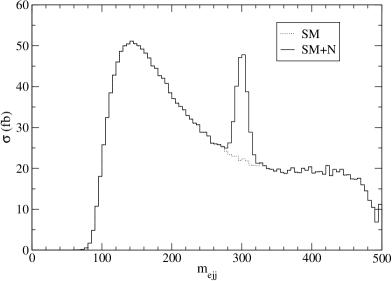
In order to discuss the ILC limits we concentrate on the lightest heavy neutrino , and follow the analysis in [1]. We omit the subindex 1 and denote the corresponding mixing matrix elements . There are two interesting scenarios: (i) the heavy neutrino only mixes with the electron; (ii) it mixes with and either , , or both. A third less interesting possibility is that the heavy neutrino does not mix with the electron. We discuss these three cases in turn. In the first two cases the heavy neutrino couples directly to the initial state , and one must search for it in its main decay mode with . In Appendix B we provide a more detailed discussion of this process. Here, it is enough to note that one has to look for a peak in the mass distribution. In Fig. 1.1 (a) we plot the invariant mass for . The center of mass energy is taken to be 500 GeV. The solid line corresponds to the SM plus a 300 GeV Majorana neutrino, being the dotted line the SM prediction. The width of the peak is due to energy smearing applied in our Monte Carlo and not to the intrinsic neutrino width GeV. We must emphasize that the total cross sections and the derived limits do not depend on the nature of the heavy neutrino, but the angular distributions do depend on its Majorana or Dirac mass character.
 |
 |
| (a) | (b) |
In Fig. 1.1 (b) we show the peak which characterizes the main SM background .
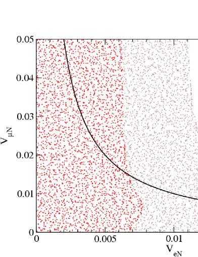
With convenient cuts on these two distributions in the different leptonic channels , , one can derive the corresponding combined limits using the signal reconstruction method explained in [43]. The integrated luminosity is assumed to be 345 fb-1, as expected after one year of running. In Fig. 1.2 we plot the combined limits on and or for the same heavy neutrino mass of 300 GeV. At the ILC the sensitivities in the muon and electron channels are similar, and both are better than in production. This can be clearly observed in both plots: a coupling has little effect on the limits on , but a coupling with the tau decreases the sensitivity, because the decays in the tau channel are harder to observe. The direct limit on , obtained here improves the indirect one (the solid line in Fig. 1.2) only for . However, as it has already been remarked, the latter is not general and can be evaded with cancellations among heavy neutrino contributions [1].
 |
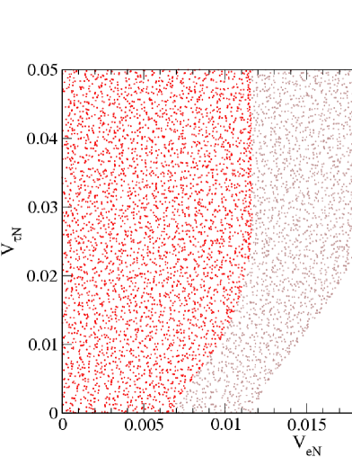 |
| (a) | (b) |
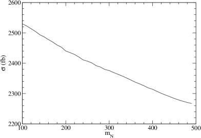
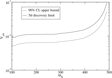
These limits are rather independent of the heavy neutrino mass. The dependence of the total cross section on can be seen in Fig. 1.3 (a), for , . For a heavier the cross sections are smaller and thus the limits on are worse. However, up to GeV this is compensated by the fact that the SM background also decreases for larger . The limits on are shown in Fig. 1.3 (b) as a function of , assuming that the heavy neutrino only mixes with the electron.
 |
 |
| (a) | (b) |
A heavy neutrino signal in the or channels is observable only if the neutrino also mixes with the electron. We now quantify this statement. We consider a heavy neutrino coupling only to the muon, with , or only to the tau, with . The beam polarisations , , opposite to the previous ones, are used to enhance the signal and reduce the SM background. The cross sections for the SM and SM plus a heavy neutrino are shown in Tab. 1.5 for these two cases. For mixing only with the muon, the statistical significance of the signal is for one year of running, and 7.3 years would be necessary to observe a deviation. If the heavy neutrino only mixes with the , the statistical significance is only , in which case a luminosity 43 times larger is required to achieve a evidence.
| SM | 1.10 | 0.389 |
|---|---|---|
| SM + | 1.20 | 0.414 |
Chapter 2 The Liquid Argon Time Projection Chamber
During the 1960s and 1970s, bubble chamber detectors [52, 53, 54] led to the discovery of many new elementary particles. Filled with a superheated liquid, the bubble chamber creates a track of small bubbles when a charged particle crosses the chamber, locally bringing the liquid to boil. Bubble chambers produce high spatial resolution pictures of ionizing events, and allow a precise investigation of the nuclear processes occurring in the medium. However, in recent times, the use of bubble chambers has been superseded by electronic detectors, since bubble chambers are difficult to trigger, and experiments with high statistics are not really practicable because of the time consuming analysis of bubble chamber pictures. The attempt to merge the superb imaging capabilities of traditional bubble chambers and the advantages of electronic read-out in a single detector led C. Rubbia to propose the Liquid Argon (LAr) time projection chamber (TPC) in 1977 [55]. The detector is essentially a cryostat filled with a liquified noble gas and equipped with an electronic readout that measures the ionization charge produced by the passage of charged particles. This detector provides three-dimensional imaging and, since the ionization charge is proportional to the energy deposition, also acts as a calorimeter of very fine granularity and high accuracy. Thus, this device is ideal to study particle interactions and does not present the problems of traditional bubble chambers, since the electronic read-out allows the self-triggering and automatic processing and analysis of the events.
ICARUS is a project, proposed in 1985 [56, 57], for the installation of a large LAr TPC in the Gran Sasso Laboratory (LNGS), Italy, for the study of neutrino physics and matter stability. Several years of R&D with prototypes of increasing size have allowed to overcome the major technological problems in the establishment of this technique.
2.1 Principles of the Time Projection Chamber
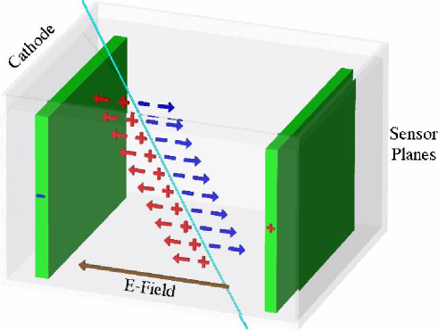
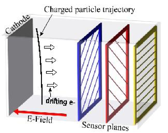
The Time Projection Chamber (TPC) is essentially a three dimensional tracking device, capable of providing imaging of an ionizing particle track and a measurement of its specific energy loss, dE/dx. It consists of a pair of parallel electrodes immersed in an ionization medium (a gas or a liquid) and connected to a high voltage power supply (see Fig. 2.1), producing a homogeneous electric field perpendicular to the electrodes.
2.1.1 Detection principle
A particle passing through the gas or the liquid will ionize the medium along the track and create ion–electron pairs (see fig. 2.1). The applied electric field suppresses the immediate recombination of the pairs (important mainly in a liquid medium), pulling the electrons and ions apart. The ionization electrons of the particle track will drift along the electric field lines to the anode, which is composed of an array of position sensitive sensors.
Imaging of events
The sensors located in the anode of the detector consist of a set of planes of multiple parallel wires (hereafter called wire planes) (see fig. 2.2) . We can obtain two-dimensional projections of the ionization point, constraining one spatial coordinate from the wire collecting the charge (or a current being induced) and the other from the drift time. In order to obtain three-dimensional coordinates, at least two wire planes with different wire orientations are necessary; therefore, the read-out system must be non-destructive.
 |
 |
The transparency of a wire plane or grid for electrons drifting along the electric field lines is a function of the ratio of the fields and , in front and behind the grid respectively, and of the ratio where is the wire radius and is the spacing between wires (pitch). Full transparency is reached when the following condition is satisfied [58]:
| (2.1) |
This condition has to be balanced against the requirement that the grid has to act as an electrostatic shielding between the space in front and behind it. If this condition is satisfied, a drifting charge will be sensed by the electrodes behind the grid only when the grid itself is crossed. Detailed calculations show that the shielding power, , of a grid is approximately given by the following formula [58]:
| (2.2) |
where is the distance between the grid and the next electrode. Note, that shielding factors deviating a few percent from 1 are acceptable.
The drifting electrons, following the electric field lines, can cross a succession of several planes of parallel tensed wires oriented in different directions (see Fig. 2.2), where the condition (2.1) is verified. The electrostatic separation between the sensing wires allows a very sharp localization of the drifting charge, hence a good spatial resolution. Each of the wire planes provides a two-dimensional projection of the event image with a common coordinate (the drift time), allowing the three-dimensional reconstruction of the event. The basic three-dimensional pixel (or “bubble”) size is determined by the wire pitch and the resolution in the drift direction. The resolution cannot be improved by arbitrarily reducing the spacing of the wires. In addition to the practical difficulties of precisely stringing wires at a pitch below , there is a fundamental limitation: the electrostatic force between the wires is balanced by the mechanical tension, which cannot exceed a critical value. This gives the following approximate stability condition [9, Eq. 28.14]:
| (2.3) |
where is the wire length, is the voltage of the sense wire and is the tension of the wire in grams–weight equivalent.
While approaching a plane, the electrons induce a current only on the wires nearby; when moving away, a current of opposite sign is induced. A detailed analysis of the induced signals for the geometrical configuration displayed in Fig. 2.2 has been performed by Gatti et al. [59]. Due to the shielding of the adjacent grids, the signals have a limited duration. Only the signals on the wires of the first grid are “prompt”, i.e. start as soon as the ionizing particle crosses the chamber, and can be used to determine the reference time for the electron drift (). The time can be also determined by the coincident detection of the scintillation light produced in the argon, using a suitable system of photomultiplier tubes.
Selection of the dielectric medium
The liquid ionization medium has the advantage of a higher density and lower diffusion compared to a gaseous medium. The higher density will permit to have an efficient target for weakly interacting particles in a relatively small volume. The high stopping power of the liquid leads to a short enough range of the (low energy) charged particles, to be fully contained in the sensitive volume. For this type of events the LAr TPC works, in addition to the imaging, as a calorimeter with fine granularity. LAr has a radiation length of 14 cm and a nuclear interaction length of 83.6 cm giving good electromagnetic and hadronic calorimetric properties. The high ionization density in the liquid gives enough electron–ion pairs per unit length to detect directly the ionization charge without any multiplication. Thus, the liquid has the advantage to give a high resolution spatial tracking information, and, at the same time, acting as a continuous hadronic and electromagnetic calorimeter. A summary of Physical and Chemical properties of argon can be consulted in Tab. 2.1.
A big difference for the signal measurement between gaseous and liquid ionization media is given by the fact that there is no charge multiplication near the sensing wires in a liquid. As a consequence of the short mean free path of drifting electrons in liquid, they don’t gain enough energy between the collisions to ionize other atoms, and thus, cannot create an avalanche. The small amount of charge (about 20 000 electrons for mips and 3 mm wire pitch) reaching the sensors must be read by a low noise preamplifier with a high gain (see Sec. 2.1.2).
| Atomic number | 18 |
|---|---|
| Concentration in air | |
| Naturally occurring isotopes | stable |
| stable | |
| stable | |
| Melting point (101325 Pa) | ℃ |
| Boiling point (101325 Pa) | ℃ |
| Density at boiling point (101325 Pa) | liquid |
| gas | |
| Liquid heat capacity at boiling point (101325 Pa) | liquid |
| Latent energy of fusion at boiling point (101325 Pa) | liquid |
| for a mip | |
| Critical energy (electrons) | |
| Mean excitation potential | |
| Energy to produce an electron-ion pair | |
| Radiation length | |
| Molière radius | |
| Nuclear interaction length | |
| Maximal breakdown strength (depending on purity level) | |
| Diffusion coefficient (89 K) | |
| Recombination factor for mips () | at |
Calorimetry and particle identification
Charged particles traversing the LAr sensitive volume produce ionization electrons in a number proportional to the energy transferred to the LAr. The ionization electrons drift along the electric field lines to the wire planes pushed by the electric field perpendicular to the wire planes, inducing a current on the wires near which they are drifting while approaching the different wire planes. Therefore, each wire of the read-out plane records the energy deposited in a segment of the ionization track. Thus, the combined spatial and calorimetric reconstructions, exploiting the fine granularity and imaging capabilities of the detector, allows the precise measurement of the energy loss per crossed distance () and hence the identification of the ionizing particle.
The complete calorimetric reconstruction of the events requires to take into account the effects of the electron-ion recombination and charge attenuation by electron attachment to electronegative impurities. Both effects reduce the amount of collected charge with respect to the one produced during the ionization. The recombination of ion-electron pairs occurs immediately after the ionization, due to their electrostatic attraction. The recombined electron-ion pairs form excited atomic states that release the energy in the form of (detectable) light. The magnitude of the recombination effect depends on both the electric field and the ionization density (). Charge attenuation is due to the attachment of the drift electrons to the electronegative impurities, and depends also on the electric field and on the concentration of electronegative impurities present on the LAr volume. The precise knowledge of these two phenomena allows their off-line unfolding from the calorimetric data.
 |
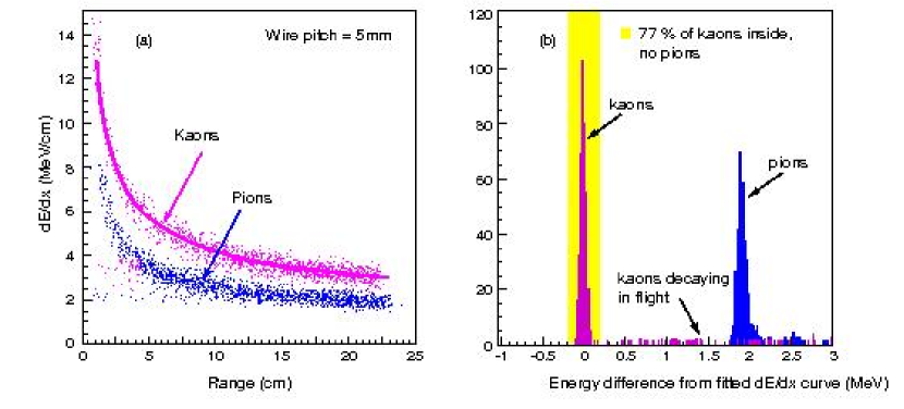 |
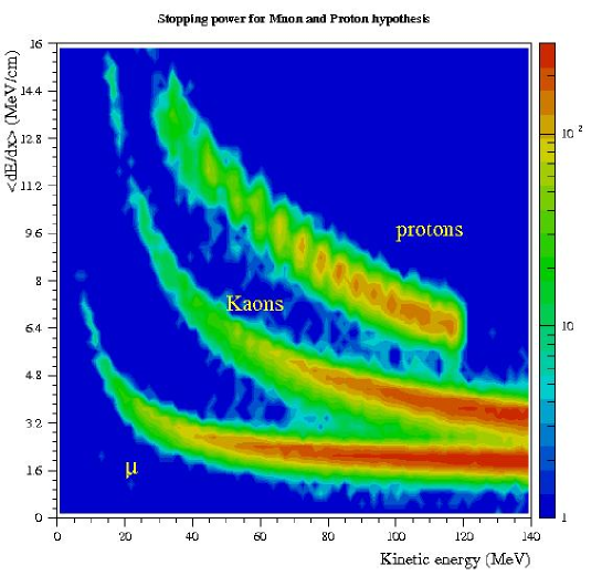
If the granularity of the read-out electrodes is high enough, a sampling of the energy loss per crossed distance () for several points along the ionization tracks is possible. If, on the other hand, the momentum of the particle is independently known, e.g. from its curvature in a magnetic field, or from its range (for particles stopping in the LAr sensitive volume only), or from multiple scattering, we can determine the mass of the ionizing particle by means of the Bethe-Bloch formula (see later section 4.6) which describes the energy loss per crossed distance (), and hence identify the ionizing particle. The particle identification capability [60] is illustrated in Fig. 2.3, where the vs. kinetic energy behaviour of stopping muons, kaons and protons (top), and a sample of stopping pions and kaons (bottom), are compared.
2.1.2 Technical considerations
The particularities of the detection technique described in the two previous sections, require special consideration of certain technical aspects, namely:
-
•
A system to provide the time of the event occurrence () is needed in order to trigger the data acquisition (DAQ) system and to determine the absolute position of the event along the drift direction.
-
•
The electronic read-out system must be capable of detecting the signal produced by a few thousand electrons.
-
•
The level of purity of the LAr must be high enough so that the signal is not strongly degraded along the drift path.
The present solutions provided by the ICARUS collaboration for each of these aspects are summarized below.
Trigger and determination
The trigger system must be suited for the rare events to be detected underground by ICARUS, and must provide the absolute time of the event occurrence. In principle, the drift time difference between any two points of the projected tracks allows to reconstruct the geometrical topology of the events. However, the absolute position along the drift direction must be known when correcting (off-line) the measured charge for the effects of the charge attenuation. A precise knowledge of is thus required to achieve a good energy resolution.
As we already mentioned in section 2.1.1, the signal on the wire plane facing the drift volume starts as soon as the ionizing particle crosses the detector, and the electron-ion pairs are formed. This feature can be used to trigger the DAQ system (hence referred as self-triggering capability) and to provide the time . An alternative system can be provided by a set of photo-multiplier tubes (PMT’s) immersed in the LAr, which detect the scintillation light produced in the LAr by the passage of an ionizing particle. Scintillation photons are produced basically by two different processes [61]:
-
•
by the direct excitation of an argon atom followed by an excited molecule formation and de-excitation:
(2.4) -
•
by the formation of a molecular state through recombination processes between electrons and molecular ions:
(2.5)
In both cases the average photon wavelength is nm, and the emission occurs within a time window which depends on the excited state. The de-excitation proceeds from two different states, with decay constants of about 5 ns (fast component) and about 1 s (slow component), respectively. The detection of the scintillation light requires the use of PMT’s equipped with suitable windows (like MgF2, that transmits UV radiation down to 115 nm), or to provide the PMT cathode with a proper wavelength shifting system. This trigger system allows the detection of cosmic ray events with energies down to a few hundred keV.
Read-out system
One of the main problems which this detection technique must cope with is the relatively small amplitude of the signals. This is due to the absence of charge amplification during the electron drift process or near the anode. Typically, 1 mm of a minimum ionizing track delivers less than electrons in LAr. The signal is even smaller at low electric fields due to the effects of the charge attenuation and the electron-ion recombination. The imaging of ionizing events requires, therefore, the use of low noise read-out electronics.
The present solution for the read-out system is the product of several years of tests and experience gained by the ICARUS collaboration on small scale prototypes [62, 63, 64, 65]. The readout system is structured as a multichannel waveform recorder that stores the charge information collected by each sense wire during the drift of the electrons at a 2.5 MHz sampling rate. Each wire module (16 wires) is equipped with a current integrating amplifier feeding a 10 bit flash ADC that samples the (multiplexed) signal with a frequency of 40 MHz.
Argon purification
In order to make long electron drift paths possible (of the order of one meter or more) LAr must be ultra-pure. An electron in the liquid undergoes about molecular collisions per second. Hence, impurities with large attachment probability must be kept at very low level, on the order or less than ppb (ppb=10-9), to achieve electron lifetimes in excess of a few milliseconds. The electro-negative impurities are mainly represented by oxygen, water, carbon dioxide and, in minor concentrations, some chlorine and fluorine compounds. If the impurity concentration is constant over the whole volume, the charge decreases exponentially with the drift time:
| (2.6) |
where is the mean lifetime of the electrons in argon. The lifetime is directly connected to the impurity concentration by an inverse linear relationship [66]:
| (2.7) |
Thus, the lifetime provides a direct measurement of the LAr impurity concentration ( equivalent).
Commercial LAr has a contamination level of the order of a few ppm (ppm=10-6) of oxygen equivalent, this corresponds to a mean lifetime of only , absolutely insufficient for a TPC. A considerable amount of R&D has been performed by the ICARUS collaboration in order to master the argon purification process [67, 68]. LAr can also be contaminated inside the cryostat, by the degassing process of those parts (walls, electrodes, cables, etc.) covered by the (hotter) argon gas. Therefore, it is necessary not only to purify the LAr before the filling of the cryostat, but also to ensure a continuous purification inside the cryostat, forcing the LAr recirculation through a dedicated purifying unit.
2.2 The ICARUS detector
The ICARUS collaboration is planning to build a large LAr TPC as a neutrino observatory and a detector to search for nucleon decays [69]. A possible detector would contain 3000 tons of LAr, divided into five 600 ton (T600) modules; each T600 module consists of two 300 ton half-modules with a common thermal insulation. The first 300 ton module was successfully tested in 2001 at the surface of the Earth in Pavia (Italy) [68]; the first T600 module is being installed at the Gran Sasso underground laboratory in Italy. The physics program contains the study of neutrino oscillations with the long base line -beam from CERN to the Gran Sasso [69] with a search for appearance, measurements of solar, atmospheric and supernova neutrinos and a sensitive search for nucleon decays.
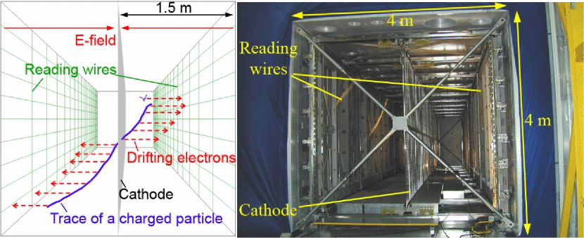
In an extensive R&D program several small scale prototypes have been constructed and operated, mainly at CERN, Pavia (Italy) and the Gran Sasso Laboratory (Italy), in order to overcome the main technological problems in the establishment of the ICARUS technology, and demonstrate many of the physics capabilities of the detector.
ICARUS T600 is a large cryostat divided into two identical, independent, adjacent reservoirs (half–modules), containing more than 300 tons LAr each (see Fig. 2.4). Both half–modules contain an internal detector (composed of two TPC’s), the field shaping system, monitors, probes and PMT’s; they are externally surrounded by a set of thermal insulation layers.
Outside the detector are located the read-out electronics (on top of the cryostat), and the cryogenic plant composed of a liquid nitrogen (LN2) cooling circuit and of a system of purifiers needed to achieve the required LAr purity.
The inner detector structure of each half–module consists of two TPCs separated by a common cathode. Each TPC is made of three parallel wire planes, 3 mm apart; the wires of the first plane are horizontal and the orientation of the two other planes is 60∘ to the horizontal direction; the wire pitch is 3 mm. The third wire plane gives redundancy data for better pattern recognition. The total number of wires in each half–module is 53 248. The read-out of the signals induced on the TPC wires by the electron drift allows the reconstruction of a full three-dimensional (3D) image of the event; the 3D reconstruction of the event is obtained by correlating the signals from the different planes at the same drift distance. Table 2.2 summarizes some technical data of the ICARUS T600 half–module (T300) detector.
| Inner dimensions | (length, width, height) |
|---|---|
| Inner volume | |
| Active111The active volumes are defined as the parallelepipeds with the side surfaces equal to the wire chamber surface and with width equal to twice the distance between the first wire plane (0 and the cathode.dimensions | (length, width, height) |
| Active volume | |
| Sensing planes | 1st Induction, 2nd Induction, Collection, 3 mm spacing |
| Channel number | 53248 wires |
| Electron drift length | |
| Maximal drift time | @ |
An uniform electric field perpendicular to the wires is established in the LAr volume of each half–module by means of a HV system, as required to allow and guide the drift of the ionization electrons. The system is composed of a cathode plane, parallel to the wire planes, placed at the centre of the LAr volume of each half-module at a distance of about from the wires of each side. The HV system is completed by field shaping electrodes to guarantee the uniformity of the field along the drift direction, and by a HV feedthrough to set the required voltage on the cathode. At the nominal voltage of , corresponding to an electric field of , the maximum drift time in LAr is about ms.
The top side of the cryostat hosts the exit flanges equipped with signal feedthroughs for the electrical connection of the wires with the read-out electronics, and for all the internal instrumentation (PMTs, LAr purity monitors, level and temperature probes, etc.). The electronic chain is designed to allow for continuous read-out, digitization and waveform recording of the signals from each wire of the TPC. It is composed of three basic units serving 32 channels:
-
•
The decoupling board receives analog signals from the TPC wires via vacuum-tight feedthrough flanges and passes them to the analog board. It also provides biasing of the wires and distribution of calibration signals.
-
•
The analog board houses the signal amplifiers, performs 16:1 multiplexing and the data conversion (10 bit) at a 40 MHz rate. Thus every channel is sampled at MHz.
-
•
The digital board uses custom programmable chips (two per board) specially developed for ICARUS, called DAEDALUS, that implement a hit finding algorithm. Each board receives the multiplexed digital data via an external serial-link cable.
Ionization in LAr is accompanied by scintillation light emission. Detection of this light can provide an effective method for absolute time measurement of the event as well as an internal trigger signal. A system to detect this LAr scintillation light has been implemented based on large surface (8 in.) PMTs directly immersed in the LAr.
The calorimetric measurement of the energy deposited by the ionizing particle in the LAr volume is obtained by collecting information from the last of the three wire planes, working in charge collection mode.
Chapter 3 The 50 liter Liquid Argon TPC
The 50 liter Liquid Argon (LAr) Time Projection Chamber (TPC) is a detector built and successfully operated at CERN for R&D purposes within the ICARUS programme. In the year 1997 it was exposed to the CERN neutrino beam for the entire SPS neutrino run period as proposed and approved at the SPSLC of January 1997 [70]. The detector, complemented with scintillators acting as veto, trigger counters and pre-shower counters, was installed in front of the NOMAD detector. The collected data brought important information for a better understanding of the performance of Liquid Argon TPC’s which should be useful for the entire ICARUS programme.
3.1 The geometrical layout
The detector structure consists in a stainless steel cylindrical main vessel, 70 cm diameter, 90 cm height, whose upper face is an UHV flange housing the feed-through’s for vacuum, liquid Ar filling, high voltages and read-out electronics (Fig. 3.1). Inside the main vessel, an ICARUS type Liquid Argon TPC is mounted. The TPC has the shape of a parallelepiped whose opposite horizontal faces (32.532.5 cm2) act as cathode and anode, while the side faces, 47 cm long, support the field-shaping electrodes (Fig. 3.2). The mass of the Liquid Argon contained in the active volume is 69 kg ( K at 1 atm, g/cm3). Ionization electrons produced by the passage of charged particles drift vertically toward the anode by means of a constant electric field of 214 V/cm.
The read-out electrodes, forming the anode, are two parallel wire planes spaced by 4 mm. Each plane is made up of 128 stainless steel wires, 100 m diameter and 2.54 mm pitch. The first plane (facing the drift volume) works in induction mode while the second collects the drifting electrons (see Sec. 2.1.1). The wire direction on the induction plane runs orthogonally to that on the collection plane. The wire geometry is the simplest version of the ICARUS readout technique [69] since both the screening grid and field wires in between sense wires have been eliminated. The wires are soldered on a vetronite frame which supports also the high voltage distribution and the de-coupling capacitors.
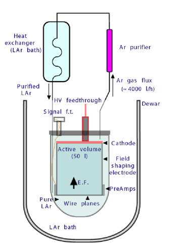 |
The cathode and the lateral field-shaping electrodes are copper strips (5 mm thick and 1.27 cm wide) positioned on a vetronite support with printed board techniques. The support was glued on a honeycomb structure to ensure rigidity. The distance between two adjacent strips is 10 mm. The 10 kV drift voltage is distributed to the strips by means of 100 M resistors. In Tab. 3.1, we have summarized the main technical data of the 50L detector.
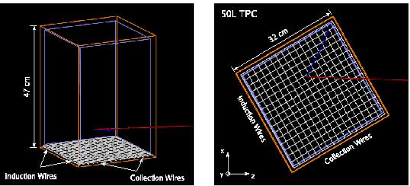 |
| Inner dimensions | (length, width, height) |
|---|---|
| Inner volume | |
| Active mass | Kg |
| Sensing planes | Induction & Collection (mutually orthogonal) |
| Wire number | 256 (128 per sensing plane) |
| Wire spacing (pitch) | |
| Wire diameter | |
| Max. drift length | |
| Electric field | |
| Signal sampling rate | @ during (=2048 time samples) |
3.2 The purification system
A crucial working parameter for a TPC operating with liquefied rare gases is the lifetime of free electrons in the medium. Primary electrons produced by the passage of charged particles drift toward the anode crossing macroscopic distances. In the present case, for an ionization electron created in the proximity of the cathode, the drift path-length exceeds 46 cm. The effectiveness of charge collection at the readout plane is related to the purity of the Argon since electron-ion recombination is mainly due to oxygen molecules present in the LAr bulk [67]. The contamination of electronegative molecules must be at the level of 0.1 ppb to allow drifts over meters.
This has been achieved using commercial gas purification systems to remove oxygen and polar molecules (H2O, CO2, fluorinated and chlorinated compounds) combined with ultra-high-vacuum techniques to avoid re-contamination of the liquid through leaks and with the use of low out-gassing materials for the detector components. Electron lifetimes higher than 3 ms (0.1 ppb) are easily and constantly reachable. Liquid phase purification allows fast filling of large detectors. Continuous recirculation of the liquid through the purifier during normal operation is used to keep the lifetime stable (against micro-leaks and out-gassing) [63, 67, 71].
As mentioned in previous Sec. 3.1, the active part of the detector is located inside a stainless steel cylinder. The connection to the outside area is obtained through a set of UHV flanges housing the signal, the high voltage cables and the vacuum feed-through. The cylinder is positioned into a 1 m diameter dewar partially filled with low purity Liquid Argon acting as a thermal bath. The ceiling of the external dewar is in direct contact with air. The level of Argon in the dewar is so small that the pure Ar in the inner cylinder can evaporate as well.
The detector is equipped with a standard ICARUS recirculation-purification system [64]. In this experiment the Argon purification is carried out in the gaseous Argon phase through the recirculation system, while during the initial filling up stage is done in the Liquid Argon phase. Once the filling up of the chamber finishes, the recirculation system takes care of increasing the purity level first and then to keep it stable during the data taking period.
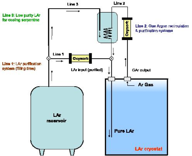
This purification procedure in the recirculation phase is outlined in a simple way as follows (see Fig. 3.3):
-
•
The gaseous Ar in the active volume crosses the feed-through and reaches an Oxisorb filter for purification, thanks to pressure gradients.
-
•
Now, the pure Argon goes through a cooling coil (inside a second buffer cooled by low-purity LAr) where it is liquefied again.
-
•
Finally, the pure LAr is collected back into the active volume.
The Argon purity is characterized by the lifetime of the free drifting electrons (), defined by:
| (3.1) |
being the primary deposited ionization charge and the electron drift time. The mean free path of these drifting electrons is nothing but the lifetime times the mean drift velocity, which have been measured in this experiment (see Sec. 5.2.1) to be 0.91 mm/s.
The purity monitor
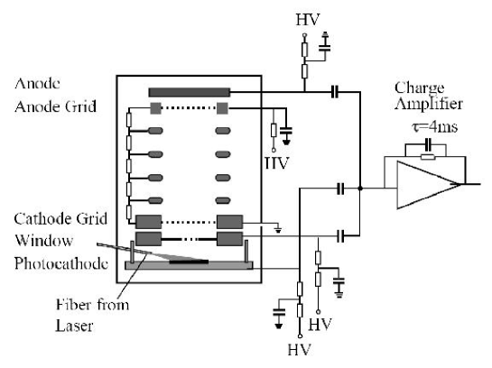
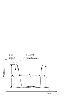
The effectiveness of the purification system through direct measurements of has been monitored during data taking by a dedicated setup first developed by the ICARUS Collaboration in 1989 [72]. It consists of a small double-gridded drift chamber located below the readout planes (see Fig. 3.4). Electrons are generated near the cathode via photoelectric effect driven by a 20 ns UV laser pulse. Each pulse produces a bunch of 107 electrons. They drift toward the anode along the electric field lines and cross a 50 cm drift region between the two transparent grids. The ratio of the induced signal in the proximity of the grids provides a real time estimate of during data taking by means of the following relation:
| (3.2) |
where is the time the drifting electrons spend from the first grid to the second, and are the time from the cathode to the first grid and to the second grid to the anode respectively.
The relation (3.2) can be understood in a very simple way: When the electrons drift between cathode and window, the amplifier receives two equal and opposite currents that cancel each other. When the electrons drift between the window and the cathode grid a positive current flows in the amplifier; as a consequence its charge output increases linearly reaching a value , the charge leaving the window. When the electrons drift between the grids, no current flows in the amplifier (at least if the grids screen perfectly). Finally when the electrons drift between the anode grid and the anode, the current is negative. The output charge signal has a negative step, whose height is the charge reaching the anode. If no charge is lost in the drift volume (zero impurity concentration), obviously ; if some charge is lost, corresponding to a lifetime the ratio of the charges is given by Eq. (3.2). In the usual case that , we have a simpler expression:
| (3.3) |
An example of the charge output is shown in Fig. 3.4 (right). From a direct measurement of the purity monitor output signal (Fig. 3.4), the collected charge , and the time intervals , and can be obtained and thus, the electron lifetime . The initial lifetime during filling was about 100 s. The recirculation/purification system, circulating about 5 liters of LAr/hour allowed to increase this value to more than 8 ms in three weeks (see Fig. 3.5). The total Argon consumption necessary to circulate the pure liquefied gas and to compensate for the heat losses was 200 liters per day.
|
|
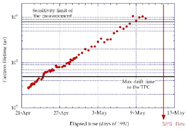
An independent estimate of can be obtained monitoring the charge attenuation for muons crossing the chamber at various heights (see Sec.5.2.2). Both methods provided consistent results and the electron lifetime averaged along the whole data taking period (9 months) turned out to be always higher than 10 ms. This performance was excellent since the maximum drift time was about 500 s and therefore the attenuation of the ionization over the drift distance can be considered negligible.
3.3 The photosensitive dopant
As we discussed before, an ionizing particle in Liquid Argon produces, along the track, electron-ion pairs and excited atoms (). The excited atoms decay, in few hundred nanoseconds, emitting ultraviolet photons with energy distribution peaked at 128 nm (9.7 eV). In the same time scale and depending on the ionization density and electric field, some of the pairs recombine also emitting UV photons. This produces saturation of the free charge as a function of the deposited energy and electric field. A possible solution to avoid this consists in dissolving in Liquid Argon a photosensitive dopant able to convert back the scintillation light into free electrons, thus linearizing the dependence of the charge on the energy and the electric field.
During this test, the Argon has been doped with Tetramethyl-Germanium as photosensitive dopant because of the following advantages [73]:
-
•
TMG is not absorbed by the Oxisorb filter in the recirculation system.
-
•
TMG can be easily purified to an electron lifetime level better than 10 s.
-
•
TMG has a large photo-absorption cross section (62 Mbarn) and large quantum efficiency (close to 100 %); this implies that small quantities ( ppm) of TMG are enough to convert all the de-excitation photons into electrons in the vicinity of the ionizing track.
-
•
TMG, at the ppm level, dissolves homogeneously in Liquid Argon.
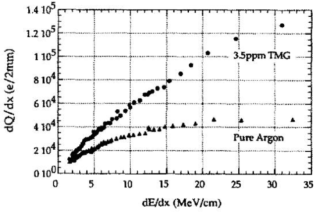
The relation between the collected charge and the energy deposition was obtained in the R&D phase of the 3-ton ICARUS prototype (see [73]) from the analysis of the stopping muon and proton events at several electric fields and TMG concentration of 1.3 ppm and 3.5 ppm. Fig. 3.6 illustrates such relation before and after the doping.
Argon excited atoms () produced by ionizing radiation lead to low excited dimer formation through collision with atoms. The rise-time corresponding to excimer formation and relaxation are in the sub-nanosecond range. For relatively low concentrations of the photodopant TMG the process which drives the recovering of drifting electrons from the scintillation light is a photoionization which follows the photoemission:
It is evident that the linearity of the detector response, after doping with TMG, is significantly improved especially at low fields where the recombination effect in pure Liquid Argon is higher. Continuous recirculation of the Argon through the purifier keeps the level of contamination stable against micro-leaks or out-gassing. Moreover no degradation of the space resolution has been measured, implying that the photo-conversion happens very close to the track.
3.4 Read-out set-up and data acquisition
The mean charge per unit pitch (2.54 mm) for a mip crossing the chamber horizontally corresponds to about electrons (4 fC) assuming no charge loss along the drift volume. The smallness of the signal and the absence of an amplification phase requires very low noise charge pre-amplifiers. This has been reached by means of JFET technology.
The pre-amplifiers
There is one preamplifier per read-out channel (256 wires), directly placed in the vetronite frame which supports also the read-out wires. Since the noise depends on temperature and input capacitance, a further improvement is obtained placing the pre-amplifiers into the liquefied gas (at -186℃). The polarization voltage (15 V) is distributed separately to each preamplifier to minimize the number of dead channels in case of failure of one of the components during data taking.
Each one of these pre-amplifiers is compound by an integrator with a time constant of and a CR output impedance with time constant of : The signal of the input current is integrated through the minimization of the input impedance in conjunction with the appropriate frequency response of the preamplifier (this minimization also allows a reduction of possible interferences between the signals of the different channels).
The amplifiers
The amplifiers gather the signal from the pre-amplifiers with typical gain of 18 and an output impedance of 120 . They are of TL.026 type, with a differential stage at the input and the output followed of a buffer stage. There were located outside the chamber at room temperature.
During the whole data taking period the amplifiers have been operating in current (or “quasi-current”) mode, which allows a rather good visualization of the ionizing events, with a signal to noise ratio of 11 for mip signals (see Fig. 3.7) and no saturation of the electronic response even in the occurrence of highly ionizing events (i.e. electromagnetic showers).
Data acquisition
The amplified signal is brought up to a set of fast 8-bit ADC (Analog to Digital Converter). The signal is sampled with a 2.5 MHz frequency for a duration of 820 s (2048 time samples), while the highest possible drift time (primary ionization at the cathode) amounts up to 500 s (1250 time samples). Once a trigger is given, the data stream is recorded into a buffer. It consists on 256 read-out channels with 2048 time samples; the signal is also recorded as an squared pulse in a virtual additional channel. The arrival of a subsequent trigger causes the switch of the data stream to another buffer (up to 8 buffers are available). The multi-buffer writing procedure minimize the dead time for signal recording to less than one sampling time (i.e. 500 s). The events are written in raw-data format without any zero suppression; they are stored locally on disk and automatically transferred to the main CERN tape facility (CASTOR) using the network.
The signal shape
With this read-out configuration the visibility of the events appeared to be optimal in both collection and induction views. In Fig. 3.7 the raw data output visualization is shown for a multi-prong neutrino event. The optimization of the analog electronic setup leads to rather clear and sharp raw images before any additional filtering algorithms were applied. Besides, the induction signal has been enhanced varying the ratio of the fields in the drift and gap regions.
The measured signals are induced by the moving charge of the drift electrons and are proportional to the drift velocity. Thus, strictly speaking the signal from the induction plane is bipolar: a small negative part from the slowly drifting electrons approaching the plane from the drift volume, and a much larger positive part induced when the electrons have passed through the plane and drift away much faster in the larger drift field among the induction and collection planes.
The careful optimization of the instrumental setup leads to a satisfactory level of performance.
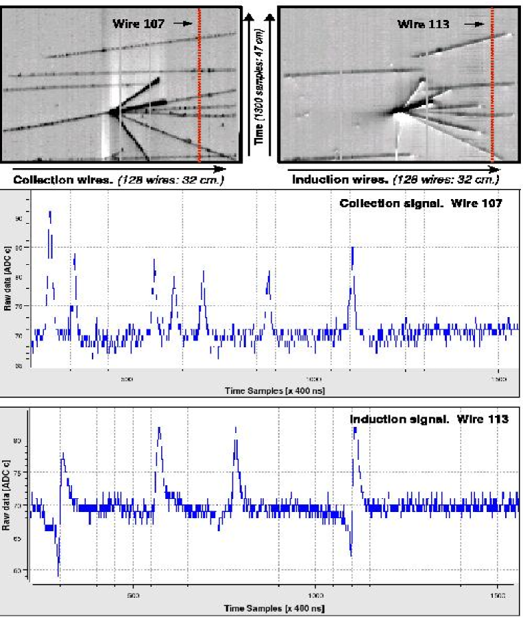 |
Chapter 4 Off-line event reconstruction
The goal of the reconstruction procedure is to extract the physical information contained in the wire output signals, i.e. the energy deposited by the different particles and the point where such a deposition has occurred, to build a complete three dimensional spatial and calorimetric picture of the event. The basic building block of a track is called hit, defined as the segment of track whose energy is read by a given wire of the readout wire planes. Therefore, the spatial and calorimetric information of the track segment is contained in the associated hit, and the sensitivity of the detector depends entirely on the hit spatial and calorimetric resolutions.
In the present chapter we describe a method developed to perform the hit spatial and calorimetric reconstruction. It is based on the pioneer work done for the stopping muon sample collected with the T600 detector [74], however many new contributions and improvements have been developed during this work in order to extend the reconstruction capabilities to low multiplicity neutrino events collected with the 50L LAr chamber (see Chapter 5).
The reconstruction algorithm proceeds through the following steps:
-
1.
Hit identification (Sec. 4.1): The hits are independently searched for in every wire as output signal regions of a certain width above the baseline output value.
-
2.
Fine hit reconstruction (Sec. 4.2): The parameters defining the hit (position, height, area), which contain the physical information, are precisely determined.
-
3.
Cluster reconstruction (Sec. 4.3): Hits are grouped into common charge deposition distributions based on their position in the wire/drift coordinate plane.
-
4.
Two-dimensional (2D) track reconstruction (Sec. 4.4): The 2D projections of the ionizing tracks are detected taking care of interaction vertexes and splitting the clusters into chains of hits with smooth transitions between them.
-
5.
Three-dimensional (3D) reconstruction (Sec. 4.5): The hit spatial coordinates are reconstructed using the association of hits from different views to common 3D track segments.
-
6.
Calorimetric reconstruction (Sec. 4.6): The spatial reconstruction of the tracks together with the information extracted from the fitting of the hits allows to precisely measure the energy deposited by a particle along its path.
In the next sections, we describe in detail the different steps of the hit reconstruction procedure.
4.1 Hit identification
4.1.1 Hit identification algorithm
The hit identification aims at distinguishing signals produced by ionization electrons from electronic noise. Hits are identified as signal regions of a certain width with output values above the local baseline (defined as the average output value in a given signal region). The hit identification algorithm typically acts over the whole wire sample of a given readout plane. In the 50L configuration there are 2 wire planes with 128 wires. Each wire is sampled 2048 times per event. The hit identification is based on basic geometrical principles of the wire signal and establishes rough preliminary bounds to the hit range along the drift coordinate, which will be of utmost importance in ulterior steps of the reconstruction procedure. No information from adjacent wires is used at this stage.
The algorithm loops over the selected group of wires (i.e. a whole wire plane), skipping those with identified problems, such as large noise conditions or disconnections, where no signal identification is possible. Hits are searched for in the wire output signal after a low frequency filter has been applied. The different steps are described in the following paragraphs.
Low & High frequency noise filter
Before the use of the hit identification algorithm is better to have the best signal we can for this purpose. In order to remove the noise contribution from the wire signals it is worth to perform a filter in frequencies. Such a filter is based on the Fourier transform of the raw wire signal. The Fourier spectrum reveals that the main contribution of drifting electrons coming from a ionizing particle to the wire signal relies on quite low frequencies. The other contributions to the read-out signal are due to electronic noise, which can be partially removed performing a suitable cut in frequencies. The Fourier transform of the wire signal in the 2048 output samples is computed using the Fast Fourier Transform (FFT) algorithm [75].
The amplitude of the low frequencies is reduced by convoluting the result with the following function of the frequency (“soft” step function):
| (4.1) |
where and are the parameters determining, respectively, the mean frequency radius and the transition region thickness. Setting the parameters to kHz and kHz effectively cuts low frequencies up to about 6.5 kHz while reducing the diffraction effect. This effect distorts the whole output range when a hit of high amplitude and sharp edges is present in the wire. The FFT filter efficiently removes the low-frequencies modulation of the signal giving as a result more uniform and constant noise baselines.
In the same way, the FFT filter is used to deal with the annoying high-frequency noise removing the contribution of waves with a frequency higher than 70 KHz. This make the search of hits much easier, above all in the case of small signals which are little bigger than the electronic noise.
Fig. 4.1 (top) shows the raw data before the application of the filter. Fig. 4.1 (bottom) shows the result of the application of the FFT filter with the cuts pointed above.
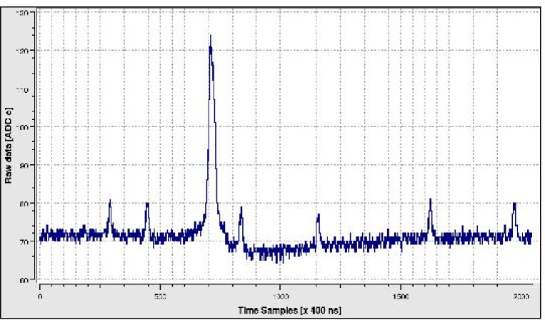
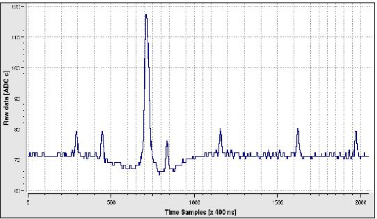
Hit search
The hit search proceeds on the filtered wire output signal. The identification is based on the geometrical features of the wire output in a given region, i.e. the presence of a relatively broad region of output values above or below the baseline. The algorithm detects the pattern of a hit in both Collection and Induction planes and determines the type of the signal shape. This is very important for the Induction plane where different patterns of signals (unipolar or bipolar) appears depending on the energy deposition. The behavior of Collection signals is always unipolar. Correlations with the signal from neighboring wires are not considered.
For every wire, the hit search algorithm follows the following steps:
-
•
Every output sample is compared with the baseline. A value above (below) the baseline by more (less) than ADC counts triggers an unipolar (bipolar) hit candidate.
-
•
The hit candidate is built with all the subsequent output samples after a threshold is given. Depending on the detected type of hit, the algorithm search for an unipolar or bipolar pattern in the wire signal.
-
•
The hit candidate is characterized by its width, i.e. the distance (in drift samples) between the hit initial and final points. Rejection of fake (noise) candidates is achieved by imposing a minimal width value.
-
•
Further rejection can be carried out depending on the expected shape of the hit. For Collection wires, where the hits are expected to have an exponential falling slope, an extra requirement on the minimum distance from the peak position to the hit end is imposed. For Induction wires, when a bipolar hit is detected we require in addition that the distance between the down and the up peak is below a minimum.
Fig. 4.2 illustrates the two different types of hits which we are dealing with and the parameters used to identify them. Fig. 4.3 illustrates the performance of the hit searching algorithm in both wire planes. It is the result of an optimized choice of the parameters for the 50L readout. As it was desired, the hit search procedure is able to detect the most of the real hits, faking as less hits as possible.
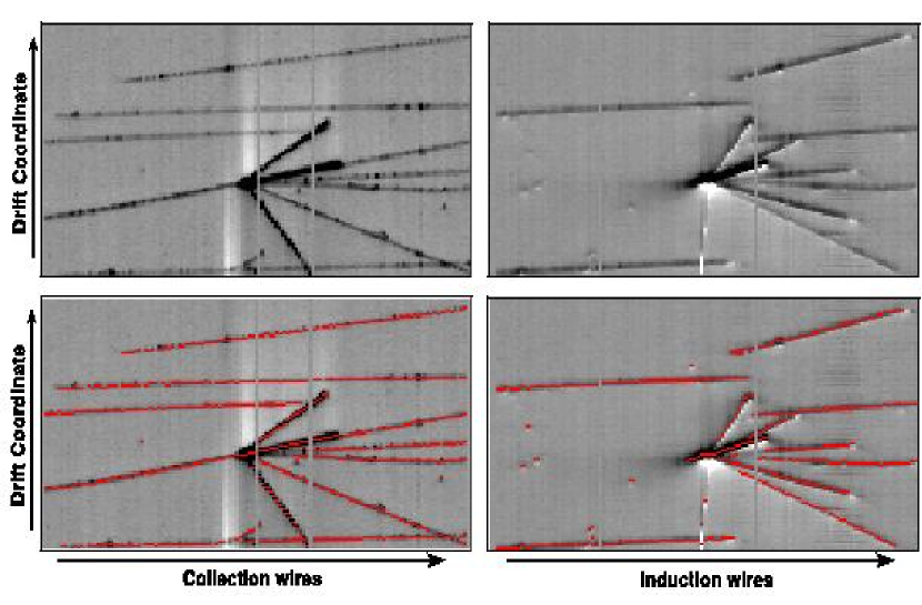
Resolving close hits
Close hits may appear when segments of tracks belonging to different ionizing particles produce a signal in the same region of the wire/drift plane (see Fig. 4.4 (left)), or when a single ionizing particle travels with small angle with respect to the drift direction (see Fig. 4.4 (right)). Identification of close hits results in a better hit calorimetric and spatial reconstruction of those tracks.
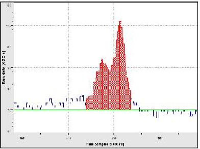
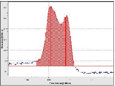
The resolution of close hits is carried out within the hit finding procedure. When a hit candidate is found, an embedded algorithm looks for patterns which point out the presence of another close hit within the hit being analyze.
In the case of Collection signals, when a falling and a rising slope are found consecutively within a hit candidate, the algorithm splits the candidate into two hits separated by the starting point of the rising slope. Although for bipolar signals in Induction wires this criteria is a little bit more complicated, the search for close hits is based on the same strategy: the presence of a close hit is found when an unexpected change of slope is find out. Once the close hits are found, the selection criteria are applied separately to both candidates.
Hit parameterization after the hit finding algorithm
After the search for hits in both wire planes they are stored together with their main geometrical features for further processing at the next stage of the reconstruction procedure.
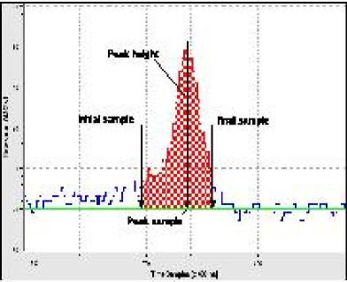
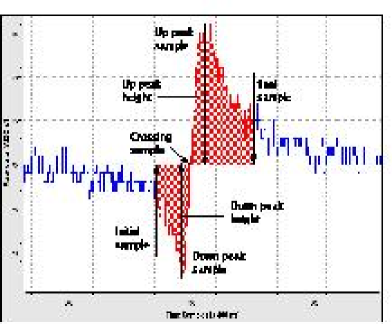
The hit identification provides the following hit parameters for unipolar signals (see Fig. 4.5 (left)):
-
•
The view and wire indexes of the hit.
-
•
The drift coordinate of the peak.
-
•
The drift coordinate range of the hit, defined by the initial and final drift samples computed in the hit expansion.
-
•
The height of the peak taken as the difference (in ADC counts) between the peak and the baseline.
In the case of bipolar signals, in addition to the these parameters, the following ones are also kept (see Fig. 4.5 (right)):
-
•
The drift coordinate of the down peak.
-
•
The height of the down peak.
-
•
The drift coordinate where the signal cross the baseline.
4.2 Fine hit reconstruction
Once the hit has been detected, a fine hit reconstruction is performed aiming at extracting in an optimal way the parameters defining the hit (position, height, area) which contain the physical information of the original associated track segment. The hit spatial reconstruction is entirely based on the determined hit peak position, whereas the hit area in Collection wires is proportional to the energy deposited by the ionizing particle, and therefore constitutes the base of the calorimetric reconstruction. In the present section we describe the fine hit reconstruction algorithm applied to the typical unipolar signals from Collection plane. No fine hit reconstruction is performed over bipolar Induction hits, and just the geometrical information from the hit identification phase is enough for the next stages of the reconstruction method.
4.2.1 Hit fit reconstruction method
The adopted approach consists of performing a fit of the output signal (the raw one) around the hit region with an analytical function that reproduces well the hit shape, and extracting the parameter values from the fitted function. The aim is to extract from them, in the most accurate possible way, the hit peak position, height and area.
The output signal within the hit window is fitted using the following analytical function of the drift time :
| (4.2) |
where is the baseline, the amplitude, the point for which the height of the function with respect to the baseline is equal to /2, and and are related to the falling and rising characteristic times, respectively (see Fig. 4.6).
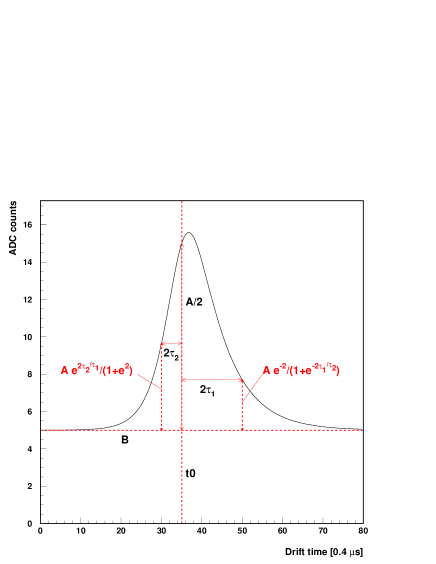
For a given hit, the values of the fit parameters are those obtained by minimizing the of the fit of to the output signal within the hit window. The minimization is performed using the MINUIT package [76].
The hit area is obtained by numerical integration of the fit function in the hit window, while the peak position () and height () are obtained analytically through the following analytical expressions:
| (4.3) |
with
Fig. 4.7 shows some examples of fitted hits corresponding to different events occurring inside the LAr active volume.
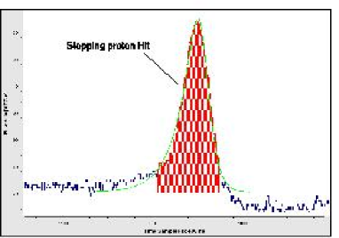 |
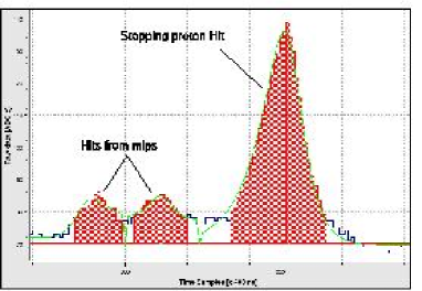 |
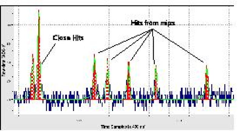 |
|
Hit parameterization after the hit fine reconstruction algorithm
The hit fine reconstruction adds the following quantities to the hits’ parameterization:
-
•
The local mean value around the hit.
-
•
The bounds of the hit window, where the different reconstruction procedures are carried out.
-
•
The peak position, the peak height and the hit area as computed by the direct ADC counting method.
-
•
The peak position, the peak height and the hit area as computed by the hit fit method.
-
•
The values of the fit parameters values.
-
•
The of the fit.
4.3 Cluster reconstruction
A cluster is defined as a group of adjacent hits within the wire/drift coordinate plane. The goal of the cluster reconstruction is to perform a first grouping of hits belonging to common charge deposition distributions, such as tracks or showers. Clusters provide identification criteria for the different patterns, and thus determine which reconstruction procedure must be followed. Clusters also provide a criterion for discrimination between signal and noise hits as well as a method to recover undetected hits through an exhaustive search.
4.3.1 Cluster reconstruction algorithm
Linking the hits
Clusters are groupings of hits which are close to each other, and two hits are close when exists a link between them. A link is defined as a pair of hits coming from consecutive wires and having overlapping drift coordinate ranges, where the drift coordinate range of a hit is defined as the one computed by the hit finding algorithm (see section 4.1). Therefore, clusters can be defined as groups of hits with links between them. The links allow to define the topological features of a hit or a hit grouping, which will be of utmost importance during the 2D and 3D reconstruction stages (Sec. 4.4 and Sec. 4.5).
To this purpose, a search for all the hits close to each other is performed, obtaining for any hit the set of those hits which are surrounding it. In such a way the links are built as logical connections between a hit and its close hits. An example of how the links are established is shown in Fig. 4.8. In terms of these links, the bounds of a cluster are defined as those hits having one link at most.
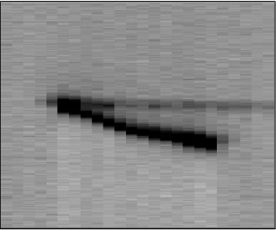
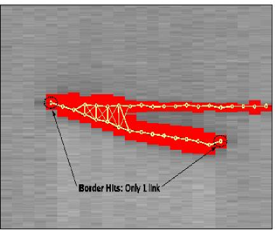
Building the clusters
Clusters are built in a two step approach. In the first step (pass I), preliminary clusters are built as groups of hits being connected by links. The second step (pass II), attempts to expand and merge together the clusters found in pass I, in order to reduce the number of the resulting clusters. The reconstruction algorithm takes as input a list of hits from a given wire plane together with their links, and constructs all possible clusters out of them, using only the information obtained by the hit finding algorithm (see section 4.1).
-
Pass I
It is essentially established above: A preliminary grouping of the hits into clusters is performed: Hits are grouped into a cluster if any of them is connected by a link with at least another one belonging to the cluster.
-
Pass II
The goal of cluster reconstruction pass II is to expand and join cluster fragments produced by pass I. It proceeds as follows: the regions around the cluster borders are examined (where a cluster border is defined as a hit linked at most with one hit within the cluster), searching for new hits which could be added to the cluster, hence reducing the cluster fragmentation caused by the misidentification of hits during the hit search phase. Attempts for clusters merging/expansion are performed both along the wire and the drift time coordinate directions.
The algorithm for the cluster expansion proceeds in the following sequential steps:
-
•
Cluster borders are identified as those hits with at most one link to the cluster.
-
•
The direction of the search is determined as wire coordinate increasing (decreasing) for borders linked with a hit from the previous (next) wire. For single hit clusters, both directions are consecutively inspected.
-
•
The slope of the search is determined as the difference between the drift time coordinates of the cluster border hit and its linked hit. For single hit clusters, this slope is equal to zero.
-
•
New hits are searched for in the consecutive wire along the determined direction using the same hit finding algorithm, but with looser parameters. Those new hits which were close to a previously existing one in the cluster are automatically joined to that cluster, creating the corresponding new link. In this way a cluster is expanded finding new misidentified hits in a clever and effective way: this exhaustive search (with loose parameters) is performed just in the region where is expected to possibly have some new hits, but not in the overall data sample like in Sec. 4.1.
-
•
The latter expansion can be continued until no more hits are found or when it reaches to another existing cluster. In this case both clusters are merged.
-
•
The borders of the new resulting cluster are identified and the whole process is repeated until no further expansion is possible.
In Fig. 4.9 the reconstruction of cluster is exemplified. In Pass I, the algorithm establishes links between the hits and construct preliminary clusters; In Pass II, the algorithm starts the exhaustive search for hits in the directions pointed by the yellow arrows (Fig. 4.9 (top)). The final result is shown in (Fig. 4.9 (bottom)), where the bigger final cluster is marked in yellow (other clusters are not shown). It is worth to underline how misidentified hits are recovered in this second pass.
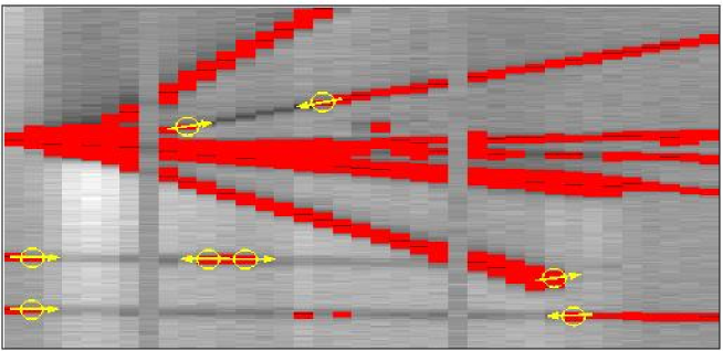
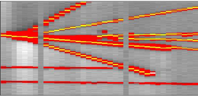
Hit parameterization after cluster reconstruction
Cluster reconstruction adds the following quantities to the hit parameters :
-
•
The cluster identification number.
-
•
The number of links associated to the hit.
-
•
The list of hits to which the hit is linked.
4.4 2D track reconstruction
The 2D track reconstruction algorithms work separately in each wire plane in order to identify the 2D projections of the real ionizing tracks. The goal is to detect smooth chains of hits which can be identify as track segments. To this purpose two different approaches have been implemented: The Tree Algorithm [77] and the Neural Network based approach [78, 79, 80]. A proper recognition of 2D track projections in both (Collection and Induction) views will lead to vertex identification and to an efficient 3D track reconstruction procedure (Sec. 4.5.3).
The description of the 2D track recognition methods and how they perform over the 50L TPC data is presented in the following sections.
4.4.1 Chains of links
Both 2D finding methods operate into each one of the found clusters (see Sec. 4.3), retrieving the information of the hits and the links between them. Since a track segment can be thought of as an unbroken chain of consecutive hits, all possible links between a hit and its adjacent are collected into chains111A chain is defined as a Collection of links consecutively connected. In principle there are many possible chains of links inside a cluster and only some of them properly define a 2D track projection. The goal of the track finding methods is to efficiently selects the real track projections from the whole sample of chains. An example of some of the chains which could be formed from the links in a cluster is shown in Fig. 4.10: The two chains at the bottom would represent real 2D track projections.
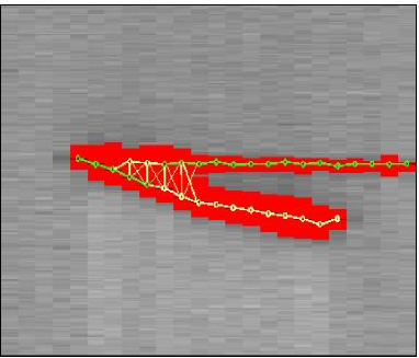 |
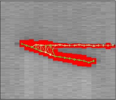 |
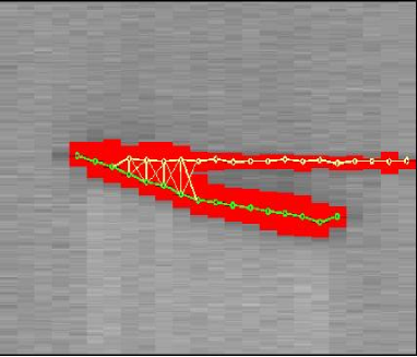 |
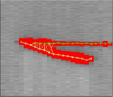 |
4.4.2 The Tree Algorithm
The Tree algorithm was successfully applied to the pattern recognition problem in multi-layer track chambers (see [77]). Because of the hits from a ionizing particle in a LAr TPC also have a layered structure (the wires readout), the approach to the track finding problem developed in [77] is directly extensible to our purposes.
The Tree algorithm works on the hits of a certain cluster using the information provided by the links and constructs from them all the possible chains (candidates to track segments) in the following way:
-
•
The algorithm starts from a link which contains a border hit (root link) and determines its elementary tree. The elementary tree of any given link is composed of this link, which is then called the trunk of the elementary tree (see Fig. 4.11 (top)), and all links having the middle hit in common and with approximately the same values of track parameters (in this case we have only one track parameter: the slope of the link). These links are then called branches of the elementary tree. Besides, all the possible elementary trees that can be consecutively connected with the starting one are also determined (see Fig. 4.11 (right)).
-
•
The collected elementary trees are connected forming the full tree associated to the root link. The links which define the limits of a full tree are called leaves (see Fig. 4.11 (bottom)). The algorithm recursively climbs the full tree from the root link, locating all chains from the root to any leaf but never finding the same chain twice. In this way tracks (or more precisely, reliable track candidates) can be recognized. Because of the branches of any elementary tree must be compatible with the slope of the trunk, any chain built in this way also have smooth transitions between their links.
-
•
The real track segment is selected from the chains belonging to the full tree by means of a selection criteria. In this case, a combination of two requirements is imposed: The longest and smoothest chain is selected as the track segment.
-
•
After the selection of the track, their links are stored, tagged and they do not participate any more in the algorithm (under the assumption that a link is never shared by two different track segments). Then, the algorithm continues processing in the same way the remaining links, starting from another root and detecting new track segments.
Examples of elementary trees are shown in Fig. 4.11 (right) The elementary trees can be combined to form a full tree as shown in Fig. 4.11(bottom). The correct track is immediately recognized as the smoothest chain of links in the full tree (chain in red in Fig. 4.11 (bottom)).
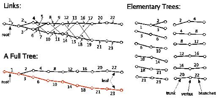
4.4.3 The Neural Network approach
The Neural Network based computing techniques are powerful tools for pattern recognition problems222See [81] for a general introduction on neural networks foundations, which have been successfully applied to many problems in experimental particle physics333See [79] for an specific discussion on particle physics problems. The track finding problem is a task of this type: given a set of hits (signals) in space, the aim is to reconstruct particle trajectories subject to smoothness constraints. The Neural Network approach for the track finding in the LAr TPC here presented is based on the work developed in [78] and [80], where an algorithm based on the Hopfield-style recurrent neural network [82] is discussed.
A neural network consists of processing units, which are called neurons, and connections between them. The state (activation) of a neuron is a function of the input it receives from other neurons. The output of a neuron is usually equal to its activation. Therefore, the state of each neuron depends on the state of the neurons from which it receives input and on the strength (weight) of these connections. Neural nets can learn representations by changing the weights of the connections between the neurons. In the following, the method specifically developed for the LAr TPC is described.
The neural network algorithm
The links between the hits in a cluster play the role of the neurons, which can be in two possible states if the link is part of the track segment and if this is not the case. The connection between the neurons (links) is established through a term called synaptic strength , which involves the link with the one. The dynamics of such a Hopfield type neural system is governed by means of the minimization of the following energy function:
| (4.4) |
The following step is to find a suitable form of the synaptic strengths which performs the required task.
Because of a track with hits can be considered as a set of links with a smooth shape and without bifurcation, the synaptic strenghts have been chosen to take care of this requirement:
| (4.5) |
where is such that short adjacent links with small relative angles are favored:
| (4.6) |
where is an odd exponent, is the relative angle between the link and the , is the length of the link and an integer (see Fig. 4.12). With this choice the energy of (4.4) will blow up for long links and large angles.

The constraint term consists of two parts:
| (4.7) |
The first term in (4.7) takes care of the requirement that there should be no bifurcating tracks: two segments with one identical index should not be “on” at the same time. This is done with the following choice for :
| (4.8) |
The other term, , ensures that the number of neurons that are “on” is roughly equal to the number of hits . It has the generic form:
| (4.9) |
This configuration of the synaptic strenghts obviously is symmetric () and with vanishing diagonal elements ().
The final expression for the energy function is:
| (4.10) |
The and factors are Lagrange multipliers entering in the definition of the energy function. At a given time the state of the system is given by the vector , while the dynamics of the system is determined by the matrix of synaptic connections. By construction, the solution of the problem of track finding is the state of the neurons which minimizes the energy function (4.10). The local updating rule which brings the system to a local minimum through the gradient descent method of the energy function is [82]:
| (4.11) |
However, in general is necessary to reach the global minimum of the system for a better performance. One way to get this is to expose the system to a noisy environment, in which the the state vector obeys the Boltzmann distribution:
| (4.12) |
where the partition function
| (4.13) |
is the sum over all possible states and is the temperature of the system.
For an efficient and fast perform of the system relaxation to the minimum, is usual to make use of the mean-field theory (MFT) approximation [83] and get for the thermal average of :
| (4.14) |
Note that the local update rule in (4.11) can be obtained from (4.14) taking the limit. can take any value between -1 and 1, and is more convenient to limit the range to the interval in other to get no contribution from deactivated neurons. To this purpose, the following linear transformation is taken
| (4.15) |
The final update rule for the neurons is obtained combining Eqs. (4.15) and (4.10):
| (4.16) |
Given an initial state of the neurons, the dynamics of the system is fully determined by (4.16).
Algorithm operation
The neural network described above can be applied to the 2D track recognition problem in a certain cluster. It takes as input the links between the hits (neurons) as they were introduced in Sec. 4.3.1 (each hit is just linked with its close hits) and, after the iteration process described by the update rule in (4.16), the set of “active” links will define the track projections. The algorithm operates as follows:
-
•
All the neurons (links) are first initialized to an active state, (4.13 (top)). This configuration performs better than a random initialization in the particular case of the interactions we have in the LAr TPC. This is because of such state is closer (in general) to the optimum state, which minimizes (4.10).
-
•
The update of the neurons is performed asynchronously through Eq. (4.16). This means that a neuron is updated after the other: the current updating neuron “sees” the other neurons in their actual state.
-
•
The process is iterated until a certain level of convergence is reached. The adopted criteria for convergence is based on the changes of the activation state of all neurons after each iteration:
(4.17) -
•
After convergence, the state of a neuron is activated if its mean value is bigger or equal than and deactivated if lower (4.13 (middle)).
-
•
Finally, the 2D tracks projection are identified as chains of consecutive activated links (Fig. 4.13 (bottom)).
There are some free parameters in the definition of the update rule in (4.16): The and factors can be modified in order to give more or less relative importance to the different terms in (4.16). The exponents in the term of (4.6) rule the smoothness requirement for the track segments. These parameters have to be defined in such a way that short and almost straight links are favored. The configuration adopted in this work is the following: , , , , which gives good quality of the results and fast convergence. However, the behavior of the network does not depend strongly on the parameters and other configurations are equally good. On the other hand, the temperature determines the speed of the convergence. High temperatures means slower convergence but gives the system more chances to scape from local minima than in the case of low temperatures.
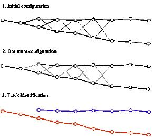
Gathered information after 2D track finding
Both methods introduced above efficiently detect 2D track segments inside a cluster of hits: tracks are recognized as chains of hits with smooth transitions (links) between them. This association of hits into 2D track structures provides a method to detect interaction vertexes in each wire plane, which will be of utmost importance at 3D reconstruction stage. Although track projections are not necessarily straight, they are fitted to a straight line which gives logical “support” and allows to extrapolate the track segments. In addition, the 2D track detection allows to assign to each hit a track identification number as well as topological information related with their surrounding hits and the track to which they belong. In such a way, a track bound can be easily defined in the same way as was done for cluster bounds (see Sec. 4.3.1): The bounds of a track are those hits having one link at most with another hit belonging to the same track (it can have however links with another hits of other tracks). Besides, a track is an unidimensional object which can be parameterized like a curve: every hit occupies a given position in the chain. In Fig. 4.14 (top-left) two tracks segments have been found in the cluster: the hits colored in green (blue) belong to the same track, in light green (light blue) the bounds of the tracks have been marked as well.
Hit parameterization after 2D track reconstruction
The information gathered by the 2D track finding procedure is stored as the following parameters in the hit structure:
-
•
The track identification number.
-
•
The number of links with other hits within the same track segment.
-
•
The list of hits to which the hit is linked within the same track segment.
-
•
The position of the hit in the track chain.
Track expanding and vertex finding
This information gathered after the 2D track finding procedure can be used to achieve two important tasks: Track expanding and vertex finding. A vertex, in a certain wire projection, can be defined as the point where two or more tracks meet. Because it is difficult to resolve the different hits in the vicinity of a vertex, in most of the cases, the track segments do not reach to the intersection of the tracks (see Fig. 4.14 (top-left)). This technical issue can be tackled in the following way:
-
•
The fitted track is extrapolated from the bound hits trying to find another track bound in its extrapolated path (Fig. 4.14 (top-right)).
-
•
If such a bound is found, the track is expanded by means of virtual hits until that bound hit (Fig. 4.14 (bottom-left)). Virtual hits (represented in pink in Figs. 4.14 bottom-right and bottom-left) are only logical and do not provide any calorimetric information, they are created to complete the geometrical reconstruction of the tracks.
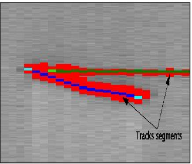 |
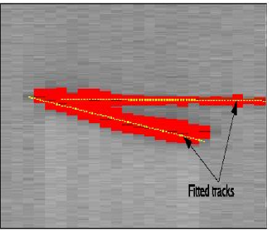 |
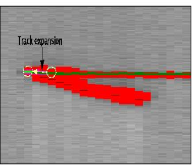 |
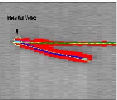 |
The latter procedure completes the 2D track finding approach in a proper way, providing the right coordinates for the track segments. Finally, vertexes are easily identified as those border hits in the track which have a neighbor which is also a border hit of another track. In Fig. 4.15, the track finding method performance is shown: The eight ionizing tracks of a deep-inelastic (DIS) neutrino event have been detected, expanded and the interaction vertex have been recognized.
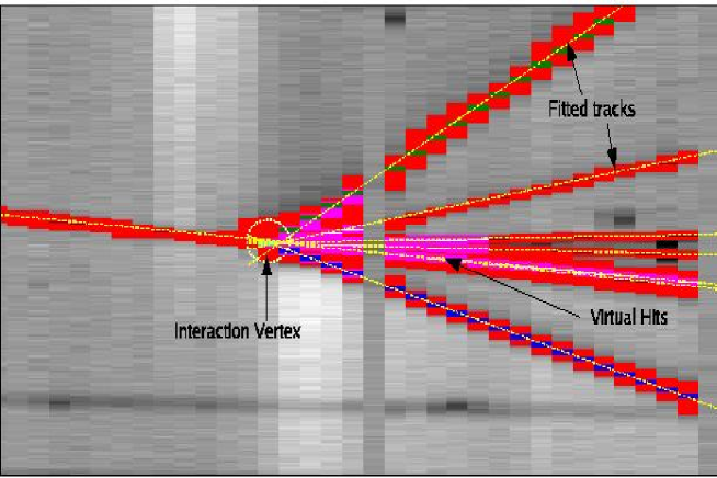
4.5 3D reconstruction
The goal of the three dimensional (3D) reconstruction is the determination of the space coordinates of the different energy deposition segments produced by the ionizing tracks traversing the LAr sensitive volume. Each wire plane constrains two spatial degrees of freedom of the hits, one common to all the wire planes (the drift coordinate) and one specific for each plane (the wire coordinate). The redundancy on the drift coordinate allows the association of hits from different planes to a common energy deposition, and together with the wire coordinates from at least two planes, allows the hit spatial reconstruction of the hit.
The 3D reconstruction algorithm developed for the LAr TPC has to different modes of operation:
-
•
The first one collects the hits within a cluster and tries to match them with the hits of complementary views.
-
•
The second one does the same, but its search of complementary hits is based on the detected 2D track segments (Sec. 4.4) of different views: it tries to match first the 2D tracks projections and thereafter match the hits belonging to them.
In the following sections we describe both approaches to the 3D reconstruction. For latter usage, we start summarizing the expressions to transform from the wire/drift coordinates system into the Cartesian system for the 50L TPC.
4.5.1 Transforming wire/drift coordinates into 3D Cartesian coordinates
We define the local Cartesian reference frame (see Fig. 4.16) centered at the bottom left corner of the electronic readout of the LAr sensitive volume. Because both the wire direction on the Induction and Collection planes run orthogonally each other, the transformation to the Cartesian reference frame is very simple. Thus, coordinates , and are associated directly to the Induction wires (in decreasing number direction), to drift time and to the Collection wires (increasing number direction) respectively. We explicitly quote below these transformations:
| (4.18) |
where the constants entering the formulae are the following: ( wires), the number of read wires in Induction plane; ( mm), the wire pitch at LAr temperature; ( MHz), the readout sampling frequency; and ( mm/s), is the electron drift velocity (see Sec. 5.2.1). Finally, , and are related to the indexes of the wires recording the hit in Induction and Collection wire planes, and the drift time coordinate (in number of samples), respectively.
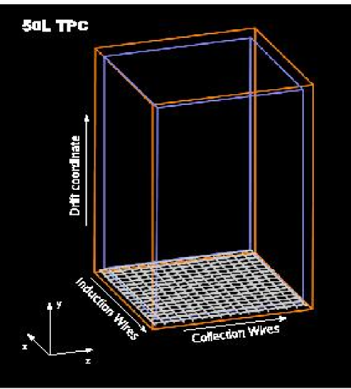
4.5.2 3D reconstruction algorithm hit by hit
The hit 3D reconstruction algorithm takes as input the sample of hits belonging to any reconstructed cluster from an arbitrarily selected view (called main view), and searches for hits from complementary secondary views corresponding to the same ionizing track segment. Such a hit is called associated hit. The combined information from a hit and its associated hit from one or more complementary views allows the determination of the hit spatial coordinates.
The algorithm proceeds in three steps (passes). In pass I, all possible associations between hits from the main and the complementary views are carried out. The associations are established based on the redundancy of the drift coordinate and the relations between hits within the clusters (links). Pass II searches for deficient associated hits, redefining their position based on the neighboring hits. Finally, in pass III, the optimal spatial coordinates for unassociated hits are computed.
Pass I
The goal of pass I is to identify the maximum possible number of associations for hits from the main view, combining single-view (links) and multi-view (associations) relations between hits.
The first and most important step is the search for associations of the cluster bound hits (i.e. hits with at most one link to the cluster). This provides a starting reference point for the association of the remaining hits of the cluster. Cluster bound hits are required to be associated to cluster bound hits from the complementary view. The remaining hits are looped over following the cluster links. In first approximation, a given hit linked to a hit is associated to a hit from the complementary view only if is linked to a hit associated to . If the previous condition cannot be fulfilled, is associated to the hit association candidate closest to .
The hit association candidates are those hits from a complementary view with equal drift coordinates (within a tolerance of drift samples) and compatible wire coordinates.
Pass II
The inefficiencies of the hit finding and cluster reconstruction algorithms (see sections 4.1 and 4.3) together with the presence of ambiguities in the determination of the hit association result in a non negligible level of bad hit associations and left-over hits after pass I.
In order to increase the hit association rate and quality, pass II searches and repairs failures on hit associations. For this, we loop over the hits starting from cluster bounds and following the links within the cluster. The following algorithm is applied:
-
•
For every two consecutive (linked) hits, and , having both an associated hit in a complementary view, the position in space of the next hits are compared to the extrapolation defined by the straight line joining and .
-
•
All hits () found until the first hit whose distance to the extrapolated line is smaller than cm are flagged for an ulterior 3D coordinates (re)assignment. Flagged hits are freed when no hit fulfilling the previous condition is found before a cluster bound is reached.
-
•
Spatial coordinates of the flagged hits are (re)computed in the following way: coordinate is computed by using the corresponding expression from Eq. (4.18); coordinates and are interpolated using the straight line parameters defined by the projection of and in the plane.
This algorithm repairs in an efficient way the position of those hits coming from straight line or small angle tracks, yielding no effect on hits coming from large angle scattering tracks. A third pass is needed in order to reduce to zero the rate of left-over hits.
Pass III
Hits remaining unassociated after pass II are reconstructed in space during pass III, in order to reach the required 100 efficiency on the hit 3D reconstruction. Pass III algorithm proceeds as follows:
-
•
Starting from every unassociated hit , the hits in the cluster are looped over, following the link path in both increasing and decreasing wire coordinate directions. For each direction, the loop continues until the first associated hit (reference hit) is found.
-
•
If reference hits at both sides of ( and ) are found before the cluster bounds are reached, the spatial coordinates of all unassociated hits between them are computed as in pass II.
-
•
If one of the reference hits is not found, the spatial coordinates of the unassociated hits are computed using a straight line extrapolation. The straight line parameters are defined by the found reference ( or ) and the closest associated hit met after following the links in the same direction we used to find the reference hit.
4.5.3 3D reconstruction by 2D track matching
This approach to the 3D reconstruction of hits is completely based on the information provided by the 2D track projection finding method. The effort spent in finding the 2D tracks leads to a very clear, simple and efficient 3D reconstruction algorithm. It works as follows:
-
•
Starting from every track segment in the main view, the algorithm tries to match the track bounds with the bounds of any another track segment in the complementary view 444Obviously, the different projections of the same ionizing track must have equal drift coordinates of their bounds (up to a difference of drift samples)..
-
•
If a complementary track is found, both projections are associated to each other and the algorithm begins the matching of the hits within the tracks.
-
•
Taking advantage of the track segments structure, the matching of the hits is performed exploiting the position of the hits within the track 555Every track has a structure defined by the chain of hits and every hit occupies a certain position in that chain (see Sec. 4.4.3).: The association of hits from complementary tracks is based on the drift coordinate like in Sec. 4.5.2 and on the relative hit position in the track. Given a hit belonging to a certain track in the main view, its associated hit is searched from the hits in the associated track in the following way: All the hits in whose drift time is compatible with the drift time of are collected; if there are more than a single candidate, the hit whose relative position in is closer to the relative position of in is selected.
In Fig. 4.17 we show an example of how this algorithm works on a low multiplicity neutrino event: Tracks projections are correctly determined in both views and then matched by time coincidences of their borders.
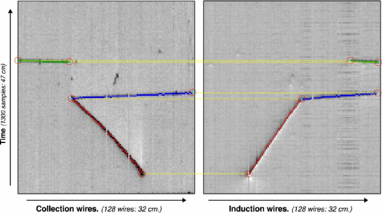
This simple algorithm has an excellent performance when the track projection segments are correctly associated. For the rest of the cases where any track segment can not be properly matched, the 3D reconstruction is performed using the hit by hit method (see Sec. 4.5.2).
Hit parameterization after 3D reconstruction
The picture of the hit is completed by adding the following information to the hit parameterization:
-
•
The associated hit(s) from the complementary view(s) and its complementary track segment (if any).
-
•
The space coordinates, , and in the Cartesian reference frame.
4.5.4 Reconstruction performance
The 3D reconstruction of hits performs efficiently on events of low multiplicity composed of several well-defined tracks (not necessarily straight). Since it is purely based on geometrical criteria, the reconstruction method is not meant to be carried out on events with more complex energy deposition patterns, such as electromagnetic or hadronic showers. For these kind of events, a method combining spatial and calorimetric relations among hits needs to be developed.
This section is essentially dedicated to present some examples of the performance of the spatial reconstruction algorithm operating on some neutrino events collected during the running of the 50L TPC exposed to the CERN neutrino beam (Chapter 5). The 3D reconstruction of a CC event with four charged particles in final state is shown in Fig. 4.18. The tools developed in this work have been successfully applied to more complex topologies, as the case of the CC event shown in Fig. 4.19, where a deep-inelastic neutrino event with eight charged particles in final state is fully reconstructed.
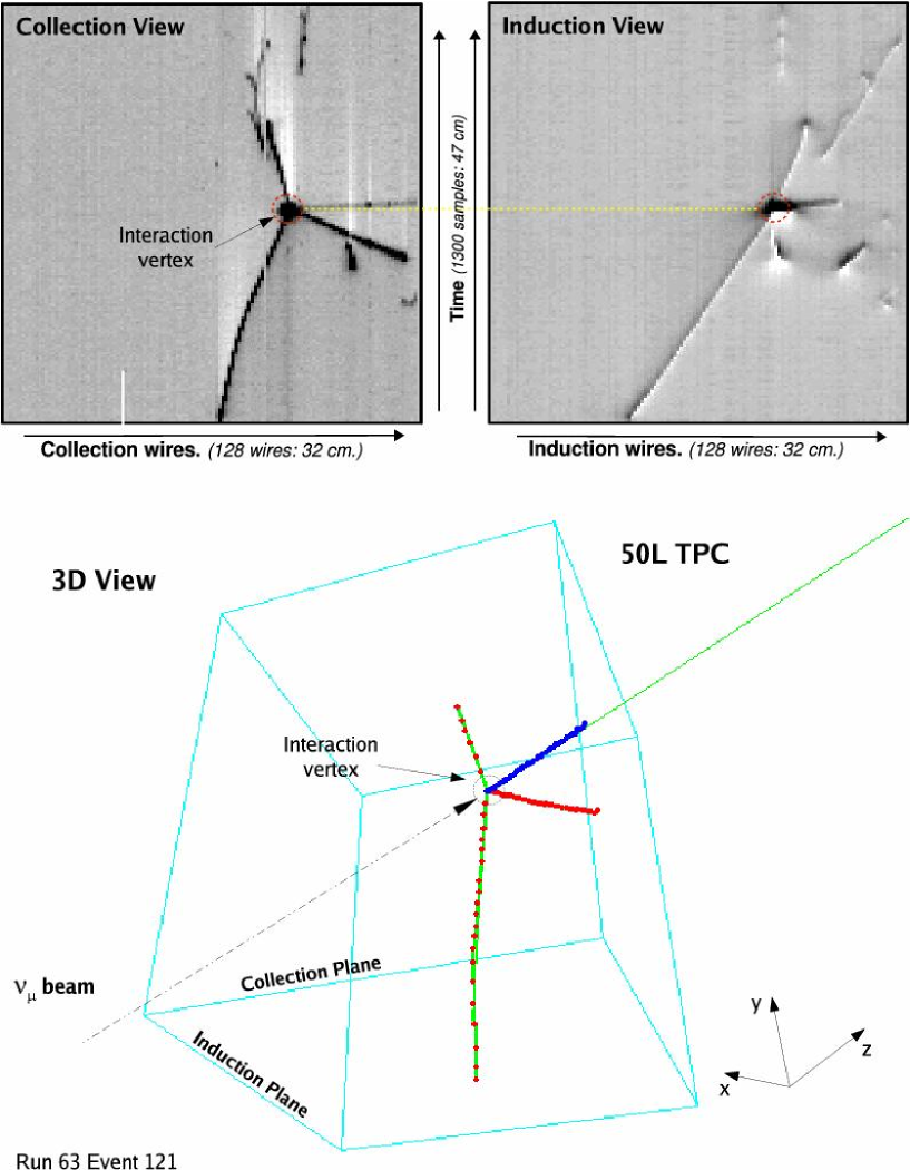
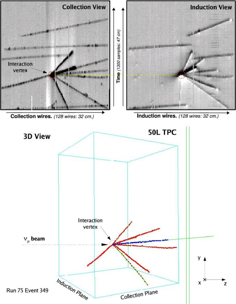
4.6 Calorimetric reconstruction
A proper spatial reconstruction of the tracks together with the information extracted from the fitting of the hits allows to precisely measure the energy deposited by a particle along its path. This capability of LAr detectors is of utmost importance since allows the energetic reconstruction of every stopping particle, as well as its identification based on the analysis of its energy loss pattern.
4.6.1 The average energy loss ()
The average particle energy loss is usually given in units of . The length unit (in g/cm2) is commonly used, because the energy loss per surface mass density with (in g/cm3) being the density of absorbing material and the length (in cm) is largely independent of the properties of the material. This length unit consequently gives the surface mass density of the material.
According to the Bethe-Bloch formula, the average energy loss is given by the following Eq. [84, 85]:
| (4.19) |
with
-
-
MeV cm2/g;
-
-
: charge of the incident particle in units of (=1 for muons);
-
-
: atomic number and atomic weight of the absorber (=18, =39.948 for argon);
-
-
: electron mass (0.511 MeV) and classical electron radius ( cm);
-
-
: Avogadro number ( mol-1);
-
-
: Ionization constant, characteristic of the absorber material (188 eV for argon);
-
-
of incident particle ();
-
-
: density of absorbing material (1.4 g/cm3 for liquid argon);
-
-
: maximum energy transfer in a single collision (see below);
-
-
: density correction (see below);
For all practical purposes, Eq. (4.19) in a given material is a function only of and only a minor dependence on (the mass of the ionizing particle) at the highest energies is introduced through . The expression as computed for muons in liquid argon is shown by the top curve in Fig. 4.20 exhibiting a minimum of 2.1 MeV/cm around 360 MeV.
The maximum transferable kinetic energy to an electron depends on the mass and the momentum of the incident particle. It can be probed that for relativistic particles ( and , with ):
| (4.20) |
Values for the density correction can be approximated by [84]:
| 0 | ||
where . The quantities and depend on the absorbing material. For liquid argon we assume the following values [86]: =0.201, =3, =3, =0.196 and =5.212.
It is also of interest to consider the mean energy loss excluding energy transfers greater than some cutoff (truncated mean energy loss) [9]:
| (4.21) |
where is the minimum between and , so that the equation reproduces the Bethe-Bloch equation for . In practice, the cut-off is given by the energy threshold for -ray detection.
Finally, in practical situations, the mean or average value is given by:
| (4.22) |
where comes from the Bethe-Bloch formula (Eq. (4.21)), and is the distance within we are measuring the energy loss.
4.6.2 The most probable energy loss ()
The energy loss distribution for thin absorbers is strongly asymmetric, due to the intrinsic statistical nature of the ionization process. The fluctuation of the energy loss around the mean value are well described by the Landau distribution [87]. According to the Landau’s theory, the probability that a singly charged particle loses an energy when traversing an absorber of thickness is expressed as:
| (4.23) |
where
| (4.24) |
is the deviation from the most probable energy loss :
| (4.25) |
where is the actual energy loss in a layer of thickness and
| (4.26) |
( in g/cm3 and in cm)
For the particular case of LAr TPC’s, is the effective portion of the track exposed to the wire, also called track pitch length.
The most probable energy loss is calculated to be [87]:
| (4.27) |
where is Euler’s constant, is the density effect and:
| (4.28) |
Therefore, for a given material the most probable value energy loss only depends on the muon momentum and on the track pitch length. Eq. (4.27) represents a very good approximation for the most probable energy loss of charged particles in thin absorbers on the vicinity () and beyond the “minimum-ionizing region”. In practice, is extracted by fitting the energy loss distribution with a Landau-Gaussian convoluted function, where the Gaussian accounts for the resolution in the charge measurement, mainly due to the electronic noise. The Landau-Gaussian convolution is defined by the following expression:
| (4.29) |
where is an overall normalization factor depending on the statistics, is the width of the convoluted Gaussian distribution, the energy and is the Landau distribution, given by Eq. (4.23).
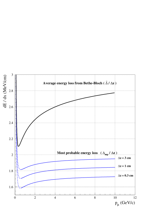
4.6.3 Average vs. most probable energy loss
In many practical situations, is necessary to parameterize the measured charge of a certain ionizing particle. In principle, we could do that by means of either or , however, the use of the mean value presents two technical problems, one intrinsic to the definition of this quantity, the other related to the limited available statistics. On one hand, the fluctuations of the energy loss are determined by a few high-energy -rays, and thus depends on the -ray detection threshold () entering expression (4.21). This quantity is not a priori known since it has a strong dependence on the performance of the spatial reconstruction algorithm. On the other hand, since strongly depends on the Landau tail, large statistics are needed in order to significantly populate the tail and hence obtain a reliable estimation of . None of the previous considerations affects the determination of .
On the other hand, the use of as energy loss estimator presents an additional problem: while is linear with the crossed distance (), as shown in Eqs. (4.19) and (4.22), behaves as , as seen from Eqs. (4.27) and (4.26). This means that the energy loss per crossed distance measured at hits from track segments of equal kinetic energy but different associated crossed distances yields Landau distributions with equal but different values. The effect is shown in Fig. 4.20, where the mean and most probable energy losses per crossed distance are plotted as a function of the muon momentum for various values.
4.6.4 Particle identification
The function (4.19) as computed for protons, kaons, pions and muons in liquid Argon, is shown by the curves in Fig. 4.21. The lines follow the expected analytical “average” behaviour only. The experimental points spread around the corresponding curve for each type of particle because of the fluctuations of the energy loss by catastrophic energy loss processes, i.e. by interactions with high energy transfers, and because of the detector resolution on the kinetic energy and measurement.
At non-relativistic energies, is dominated by the overall factor and decreases with increasing velocity until about (or ), where a broad minimum of ionization is reached (a particle at this point is known as a mip).
From the figure, it is clear that for energies below the minimum ionizing value, each particle exhibits a curve which, in most cases, is distinct from the other particle types because of the mass difference. This is precisely the characteristic that has been exploited in this work as a means for identifying particles in this energy range.
The minimum value of is almost the same for all particles of the same charge and, as the energy increases beyond this point, the term becomes almost constant and all curves seem to converge together to very similar values. As soon as the detector resolution on the measured kinetic energy and on the track pitch are taken into account, the fact that all particles behave so close above the m.i.p. region independently on the mass, make them indistinguishable by means of the technique.
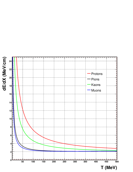
4.6.5 Energy calibration
The energy calibration consists of transforming the charge associated to a hit into energy units. The ionization charge is precisely measured in the Collection wire plane (see Sec. 4.2). The energy associated to a given hit is:
| (4.30) |
where is the calibration factor; is the average energy needed for the creation of an electron-ion pair (i.e. 23.6 eV); is the electron-ion recombination factor and is the corrected charge by the electron lifetime from Eq. (3.1) in Sec. 3.2. The calibration factor converts the detector measuring units (ADC counts) into charge units (fC), while the recombination factor depends on the absorber medium, on the applied electric field and on the density of released charge, i.e. on .
Thus, the energy calibration consist on determining and finding a suitable model which describes the recombination factor for a given detector configuration.
The electron recombination factor
Ionization electrons produced by the passage of a charged particle through the LAr volume have a non negligible probability to recombine with one of the positively ionized atoms. In such a case, the energy released in the ionization appears in the form of photons and we say that the drift electrons have been quenched. The recombination probability depends on the absorber, on the applied electric field, and on the density of released charge, i.e. on . This dependence may be intuitively understood as follows: the higher the field the faster the electrons and ions are separated, and the less time is available for the recombination; on the other hand, the larger the , the higher the number of neighbouring positive ions which are available for an electron to recombine.
The dependence of with can be modeled by Birk’s law [88] which has been successfully applied to LAr detectors in [89]:
| (4.31) |
being the pure Bethe-Bloch ionization loss, and are constants depending on the applied electric field and is the Birks coefficient accounting for quenching due to recombination. The recombination factor is the ratio between the measured and the produced (theoretical) charge:
| (4.32) |
Therefore, Eq. (4.31) can be rewritten in terms of the recombination factor by noting that has units of charge per energy, so that it can be expressed as the inverse of the factor (see Eq. (4.30)) times a dimensionless multiplicative constant () ranging between 0 and 1. Multiplying both sides of the equation by and dividing by we obtain:
| (4.33) |
A precise knowledge of the recombination factor is of the utmost importance since it determines the absolute energy calibration of the detector.
In Sec. 5.2.4, we present the analyses for the energy calibration for the 50L LAr TPC.
4.6.6 Measurement method
From the previous discussions, it is clear that the determination of the energy loss per crossed distance can be obtained by means of the measurement of the deposited energy for every hit together with the calculation of its associated track pitch length. In the following we discuss some aspects of the procedure to achieve this task in the framework or LAr TPC detectors.
The track pitch length
The length of the track portion associated to a hit (hereafter called the track pitch length: ) depends on the wire pitch and the orientation of the track with respect to the wire plane. It can range from the wire pitch length (for track pieces parallel to the wire pitch direction) to distances of the order of the chamber’s side (for tracks perpendicular to the pitch direction). Thus, the track pitch length can be written in terms of the track direction in a given hit:
| (4.34) |
being the wire pitch and the angle between the track at the hit position respect to the direction of the wires (see Fig. 4.22).
Track segmentation
In order to make an estimation of the track pitch length at any given hit belonging to a track, a partition of the track into segments of a certain number of hits is performed. Since a track is not straight in general, the aim of this procedure is to obtain a parameterization of the trajectory of the track in terms of straight line segments, which locally approximate the real track direction. Given a certain track segment with hits belonging to it, its direction is determined by fitting a three dimensional straight line to these points. Besides, an additional constraint is imposed to this fit: any track segment uses the result to the fit of the previous calculated one in order to have smooth transitions between the different parameterized lines, i.e. the fitted lines belonging to consecutive segments must have one point in common. As a result, we obtain a partition of the track trajectory into straight segments, which are consecutively connected defining a trajectory (see Fig. 4.22).

The direction associated to any track segment is determined by the parameters entering in the linear fitting, given in terms of a unit vector , or in terms of the angles and
| (4.35) |
where the index may refer to a hit or a segment, and is the corresponding associated direction vector.
Range determination
The segmentation procedure also provides an optimal method to compute the track range666The distance a particle can penetrate before it loses all its energy.. From a theoretical point of view, the mean range for a stopping particle might be calculated through the integration of the Bethe-Bloch formula (4.19) along the particle’s path:
| (4.37) |
where integrations limits go from the initial point with kinetic energy until the stopping point. If one assumes that the energy loss is continuous, the distance a particle can penetrate before it loses all its energy is a well defined number, the same for all identical particles with the same initial energy. Fig. 4.23 shows the energy–range curves for different particles calculated by a numerical integration of the Bethe-Bloch formula, which yields the approximate path length traveled. As in the vs. kinetic energy case (see Fig. 4.21), the curves give the expected “average” behavior.
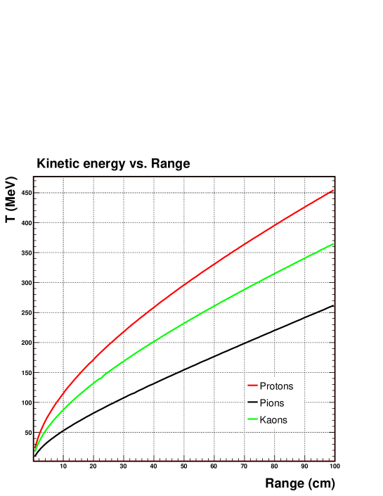
The definition of a range is complicated because of the multiple Coulomb scattering in the material and catastrophic energy loss processes (both ignored in Eq. (4.37)), which cause the particle to follow a zigzag path through the absorber and lead to substantial range straggling. The range, defined as the straight-line length, will generally be smaller than the total zigzag path length. The track segmentation method leads to a better estimation of the “real” range:
| (4.38) |
being the straight-line length of each one of the segments composing the track, and the total number of such segments.
Chapter 5 The 50L TPC exposed to The CERN Neutrino Beam
Within the broad physics programme of the ICARUS project, an important issue is the study of oscillations through the detection of accelerator neutrino interactions. The possibility to observe and by means of kinematic criteria is known to be limited, among others, by the knowledge we have of nuclear effects (Fermi motion, nuclear re-scattering and absorption, etc.). Therefore it is very important to acquire experimental data in order to tune the existing Monte-Carlo models. In addition, the exposure of a LAr TPC to a neutrino beam is mandatory to demonstrate the high recognition capability of the technique and gain experience with real neutrino events.
In 1997, the ICARUS collaboration together with a group from INFN and Milano University [90] proposed to expose a 50 liter LAr TPC to the multi-GeV wide band neutrino beam of the CERN West Area Neutrino Facility (WANF) [91], during the NOMAD [92] and CHORUS [93] data taking. The test was part of an R&D program for a medium baseline appearance experiment [94]. The idea was to collect a substantial sample of quasi-elastic (QE) interactions ( + n p + ) to study the following physics items:
-
•
Measurement of the acoplanarity and missing transverse momentum in events with the -p topology in the final state, in order to assess Fermi motion and proton re-scattering inside the nucleus.
-
•
Appearance of nuclear fragments (short tracks and blobs around the primary interaction vertex) in quasi-elastic events.
-
•
A preliminary evaluation of e/ and e/ discrimination capability by means of the specific ionization measured on the wires at the beginning of the candidate track. This measurement is limited by the size of the chamber.
The data collected in 1997 offer the unique opportunity to study nuclear effects in the Argon nucleus and to assess the identification and reconstruction capability of a LAr TPC for low-multiplicity neutrino events. The work presented in this thesis shows, for the first time, a comprehensive set of results from the 1997 test (see [95, 96, 97, 98] for preliminary results). The structure of the chapter is as follows: the experimental setup and the calibration measurements of the 50 liter TPC are discussed in Sec. 5.1 and Sec. 5.2, respectively. At the beginning of Sec. 5.3 the event reconstruction and particle identification are detailed, thereafter the analysis of a golden sample of quasi-elastic charge current (CC) interactions is presented together with a comparison with theoretical expectations. Finally, in Sec. 5.4 we measure the quasi-elastic cross section for CC interactions.
5.1 The experimental setup
The LAr TPC was placed on a platform 4.5 meters above ground, right in between the CHORUS and NOMAD detectors (Fig. 5.1). Full details of the geometrical and technical features of the 50L TPC have been treated in Sec. 3.1. As mentioned there, the active part of the detector is located inside a stainless steel cylinder. The connection to the outside area is obtained through a set of UHV flanges housing the signal, the high voltage cables and the vacuum feed-through. The cylinder is positioned into a 1 m diameter dewar partially filled with low purity Liquid Argon acting as a thermal bath and it is rotated 30∘ along the vertical axis with respect to the nominal beam direction to reduce the number of particles crossing just one readout wire.
The modest size of the LAr TPC fiducial volume (50 liter), coupled with the high energy of the WANF beam (Sec. 5.1.1), made necessary a muon spectrometer downstream the TPC. The NOMAD detector was the perfect choice to achieve this task: A coincidence with the NOMAD DAQ was set up to use the detectors located into the NOMAD magnetic dipole as a magnetic spectrometer (Sec. 5.1.2). The experimental setup was completed with additional counters for the trigger and veto systems (Sec. 5.1.3).
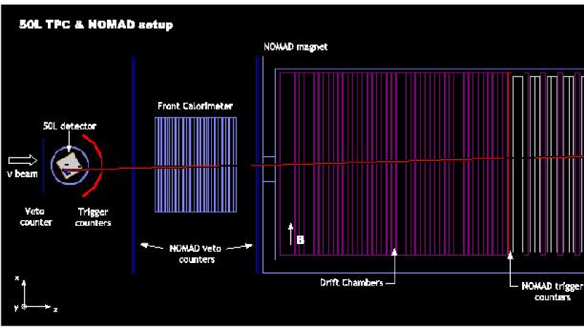
5.1.1 The Neutrino Beam
The chamber has been exposed to the beam produced at the CERN West Area Neutrino Facility (WANF [91, 99]). The geometry of the WANF is shown in Fig. 5.2. The Super Proton Synchrotron (SPS) at CERN supplied a beam of 450 GeV protons which was directed onto a beryllium target, thereby producing a large number of secondary hadrons. In every accelerator cycle (14.4 s) the protons used to produce neutrinos were extracted from the SPS in two spills, which were separated by 2.7 s. Each spill had a full width at half maximum of 3 ms and contained about protons. The number of protons incident on the target was monitored by a beam current transformer (BCT). The number of produced neutrinos was often expressed in units of protons on target (pot).
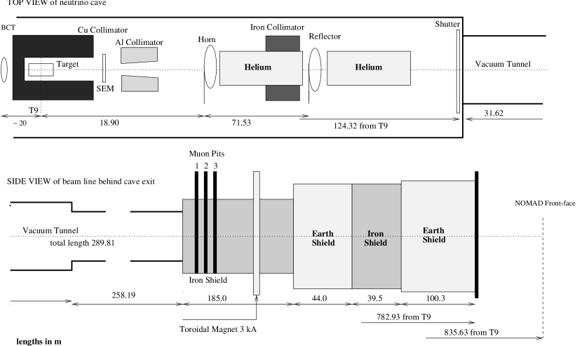
The multiplicity and charge asymmetry of the secondary particles were measured by secondary emission monitors (SEMs) placed before and after the target. The beam focusing elements, downstream of the target, were large magnets, designed to collimate the positively charged secondary particles, while deflecting the negatively charged particles away from the beam axis. Most of the focusing was done by the first element, called the horn. The second element, the reflector, focused the smaller angle particles which had been missed by the horn. Two helium bags were installed in order to increase the neutrino flux by reducing multiple scattering and secondary interactions along the beam. Downstream of the focusing elements was a vacuum decay tunnel of 290 m length in which the positively charged particles could decay and, thereby, produce the neutrinos. The major contributions to the flux came from the reactions:
The charge conjugate reactions also occurred, giving rise to a component in the beam. Earth and iron shielding directly after the decay tunnel filtered out all but neutrinos and some muons. Silicon detectors in several pits within the shielding region measured the muon multiplicity and could be used to monitor the beam and determine the absolute flux. An additional toroidal magnet, which was placed after the muon pits, deflected most of the remaining muons. The resulting neutrino beam reached the NOMAD detector 835 m downstream of the proton target with the composition and properties shown in Fig. 5.3 and Tab. 5.1 [99]. The predictions of the neutrino fluxes are based on Monte Carlo simulations. For further reference on the WANF layout and the alignment procedures, see [100].
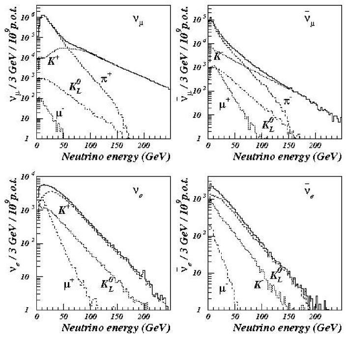
| Neutrino | Neutrino | Source | ||||||||
| Species | Flux | or | or | or | ||||||
| Rel. Abund. | ||||||||||
| 1.0 | 24.3 | 90.4 | 19.1 | 9.5 | 73.0 | 0.1 | 26.8 | 0.1 | 11.4 | |
| 0.0678 | 17.2 | 84.0 | 13.8 | 12.8 | 38.1 | 1.9 | 26.9 | 1.2 | 17.0 | |
| 0.0102 | 36.4 | - | - | 68.0 | 41.8 | 17.8 | 30.3 | 13.6 | 16.8 | |
| 0.0027 | 27.6 | - | - | 25.1 | 22.8 | 68.2 | 30.4 | 3.5 | 11.1 | |
The mean energy of the reaching the detectors is 24.3 GeV when integrating over the active NOMAD area ( ), while contamination from other flavors are below 7% for and % for [99]. Being the TPC centered on the beam axis and covering a smaller surface, a harder neutrino flux is expected, with a mean energy of 29.5 GeV (see Fig. 5.4).
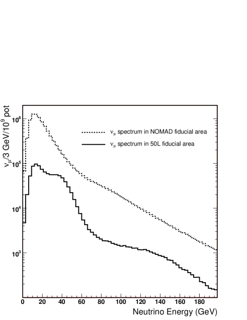
5.1.2 The NOMAD detector
The NOMAD detector [92] was composed of several independently working sub-detectors. A schematic view of the detector is shown in Figure 5.5 along with the coordinate system. The sub-detectors were placed along the beam-line with positional sensitivity transverse to the beam direction. The veto system upstream of the detector allowed a fast identification of muons entering the detector. Following the muon veto, there was the forward calorimeter (FCAL) which was used as a target for studies requiring very high statistics while sacrificing some resolution in the vertex finding. The drift chambers (DCH) in the center of the detector served both as an active target and a very precise tracking device; hence the most interesting of the detected interactions occurred there. Further downstream, the trigger planes, the transition radiation detector (TRD), the preshower (PRS) and the electromagnetic calorimeter (ECAL) were situated. These inner detectors (DCH to ECAL) were all surrounded by the old UA1 dipole magnet which provided a constant magnetic field of Tesla. The hadronic calorimeter (HCAL) followed downstream of the inner detectors and at the very end there were the muon chambers. The and axes of the co-ordinate system were centered in the middle of the first drift chamber. The neutrino beam entered with an angle of 42 mrad with respect to the axis.
In what follows, we describe some of the NOMAD subdetectors that were key for the experiment and the analyses described in this work.
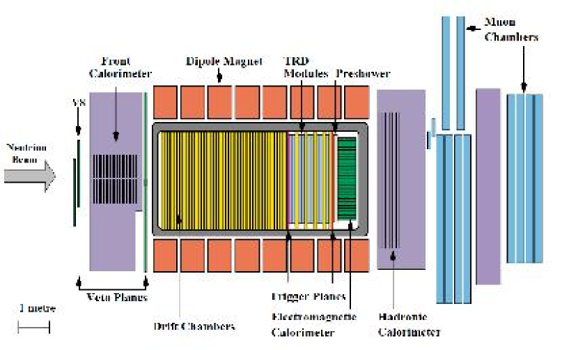
The Veto Counters
Being the most upstream detector, the veto consisted of 59 scintillator counters and covered an area of . It was used to detect muons traveling with the neutrino beam and charged particles from upstream interactions, and prevented them from causing valid triggers. An additional veto plane was positioned between the FCAL and the DCH. Charged particles from interactions downstream of the veto, e. g. in the magnet coil or the support structures of the drift chambers, were removed during analysis by constraints on the vertex position.
The scintillators were read out by photo-multipliers and a veto signal was constructed from a logical OR of all the individual counters. The efficiency of the veto was constantly monitored and found to be stable at about . The contribution of the veto to the overall dead time of the experiment during the two neutrino spills amounted to about 4 %. A detailed description of the veto system can be found in [101].
The Forward Calorimeter (FCAL)
The forward calorimeter, being the instrumented front pillar of the magnet, was used as a massive active target and allowed neutrino physics studies including di-muon production and neutral heavy lepton searches. The FCAL consisted of 23 iron plates, which were 4.9 cm thick and separated by 1.8 cm air gaps. The first 20 gaps were instrumented with scintillator counters. The dimensions of the scintillators were . Five consecutive counters along the beam direction were bunched together via light guides to form a module which was read out at both ends by photo-multipliers (see Figure 5.6). Ten such modules were arranged vertically to form a stack. There were four stacks aligned along the beam axis. The active region of the FCAL had a mass of 17 tons, was about 5 nuclear interaction lengths in depth and had an active area transverse to the beam of . Further details can be found in [92].
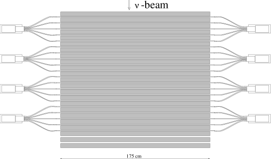
The Drift Chambers (DCH)
A crucial part of the detector were the drift chambers which provided at the same time the target material and the track and vertex reconstruction of the charged particles. The full drift chamber region consisted of 11 modules, each made up of four individual drift chambers (composed of low density, low atomic number materials). In addition to these 44 drift chambers, there were another 5 chambers in the TRD region, providing additional tracking. The chambers were filled with a mixture of argon (40 %) and ethane (60 %), and equipped with sense wires. The volume with maximal acceptance and reconstruction efficiencies was referred to as fiducial volume and had the dimensions of with a mass of 2700 kg. The overall density of was about equal to the density of liquid helium.
The sense wires in the three gaps of a drift chamber were oriented with -5, 0 and +5 degrees with respect to the magnetic field direction, corresponding to the NOMAD axis. The three ionization signals produced by a particle traversing a drift chamber allowed a hit positioning accurate to about 1.5 mm in the direction, due to the angles between the wires. Transverse to the wires ( direction) a position accuracy of was reached by the separation of the wires and a constant gas drift velocity. The position along the beam line ( direction) was determined by the position of the wire planes which was constantly monitored. The efficiency of each wire to record a hit was typically 97 %. The three dimensional information from each drift chamber could be used to reconstruct the helical path of charged particles through the magnetic field. The curvature allowed the measurement of the momentum of the particles through the relation
| (5.1) |
where is the momentum and the charge of the particle, the pitch angle of the helix, the radius of curvature and the magnetic field. The momentum resolution was a function of the particle momentum and track length. For muons and charged hadrons with normal incidence to the measuring planes the momentum resolution could be parametrized by
| (5.2) |
with
| (5.3) |
and denoting the length of the track. The first term in Eq. (5.2) corresponds to the error due to multiple-scattering, the second term arises from the single hit resolution. A detailed description of the drift chamber is given in [102].
5.1.3 The Trigger and Veto system for the 50 liter set-up
The trigger is provided by a set of scintillators located between the chamber and the NOMAD apparatus (Fig. 5.1). Each of the 3 trigger scintillator counters has a dimension of 11027 cm2. They were positioned in a half-circle 60 cm beyond the center of the chamber. Incoming charged particles are vetoed by 5 scintillators mounted in front of the chamber, 50 cm before its center, and by the last scintillator plane of CHORUS. The latter vetoes particles deflected by the CHORUS magnetic field entering the chamber at large angles with respect to the nominal beam direction.
The trigger requires the coincidence of the SPS beam spill and at least one of the trigger scintillators, vetoed by the scintillators put in front of the chamber and the CHORUS plane. This trigger is put in coincidence with the two trigger scintillator planes of NOMAD (T1 and T2 in Fig. 5.1) [101]. Moreover, a trigger is rejected if the NOMAD acquisition system is in BUSY mode or if the delay with respect to the previous trigger is lower than 500 s (“drift protection”)111This condition inhibits the occurrence of event overlaps in the multibuffer readout system..
The request of a charged particle triggering the chamber locally and reaching NOMAD up to T1 and T2 inhibits the acquisitions of neutral-current and charged-current events, limiting the sample of the present test to charged-current interactions. The trigger efficiency has been monitored during data taking through a dedicated sample of through-going muons. It turned out to be 97% averaged over the whole data taking period.
5.2 Calibration of the TPC
5.2.1 Measurement of the electron drift velocity
A fundamental parameter for the reconstruction of ionizing events occurring inside the fiducial volume of the 50L TPC is the velocity of the drifting electrons.
An absolute determination of the drift velocity and its uniformity along the fiducial volume of the chamber has been obtained exploiting the external scintillators and the additional information from NOMAD. A dedicated trigger selecting through-going muons (“mip sample”) has been put into operation adding two additional scintillators (3030 cm2) before and after the external dewar. The relative position of the chamber with respect to the NOMAD reference frame has been obtained by residual minimization of the track parameters recorded both by the TPC and the NOMAD data acquisition system. The drift velocity is obtained by fitting the absolute vertical position of the muon as reconstructed by NOMAD trackers versus the drift time measured locally by the TPC (Fig. 5.7). The corresponding drift velocity is
| (5.4) |
The measurement of the drift velocity is essential because it defines the “pitch” in the drift coordinate: Since the signal is sampled with a 2.5 MHz frequency for a duration of 820 s (2048 time samples), the drift pitch amounts up to 0.36 mm. The maximum drift distance of 47 cm is covered by a drifting electron in 520 s.
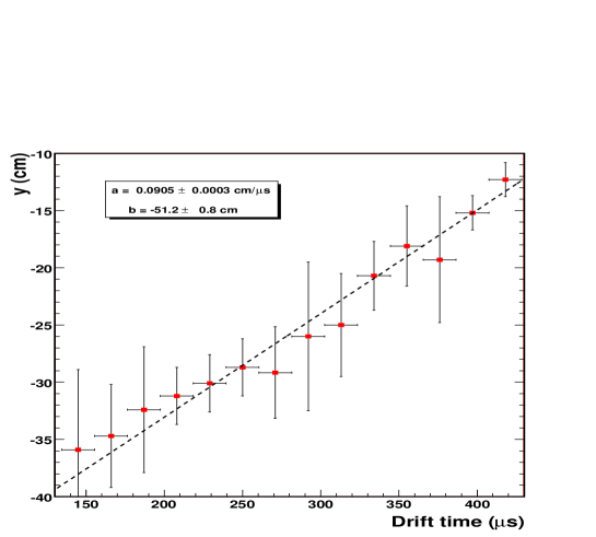
5.2.2 Measurement of the electron drift lifetime
The attenuation of the drifting electric charge towards the anode is a crucial working parameter for the TPC. It essentially depends on the purity levels in the Liquid Argon and on the applied electric field. Thanks to a purity monitor placed within the pure LAr bath (see Sec. 3.2), it was possible to obtain direct measurements of the drifting electron lifetime . During the data taking period the impurity levels of oxygen kept themselves stable, getting values of higher than 10 ms.
In this section, we perform an independent measurement of based on the spatial and calorimetric reconstruction of a sample of muons crossing the chamber at different heights (see Fig. 5.8). This sample of muons was gathered from the data collected during the exposition to the WANF beam, by means of an automatic scanning and reconstruction algorithm. Over the whole data, the algorithm was able to collect a big enough number of correctly reconstructed through-going muons. They are essentially muons coming from CC interactions occurring before the fiducial volume of the TPC, uniformly distributed in height and crossing the chamber with an approximately constant value of their drift coordinates.
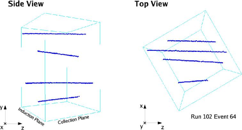
The spatial and calorimetric reconstruction tools allows to measure the energy loss per crossed distance () hit by hit for every muon (see Sec. 4.6 and Eq. (4.36)). The most probable value () is used as a suitable estimator of the energy loss for each one of those muons (see Sec. 4.6.2). As it was already discussed in Sec. 4.6.3, depends on the crossed distance associated to the sampling hits of the track, but shows a slight dependence on the kinetic energy. Being the sample of mips used in this analysis horizontal and straight muons coming in the beam direction, their track pitch length hardly varies from the mean value: . The latter ensures that the expected is essentially the same for all the muons in the sample (see Fig. 5.9).
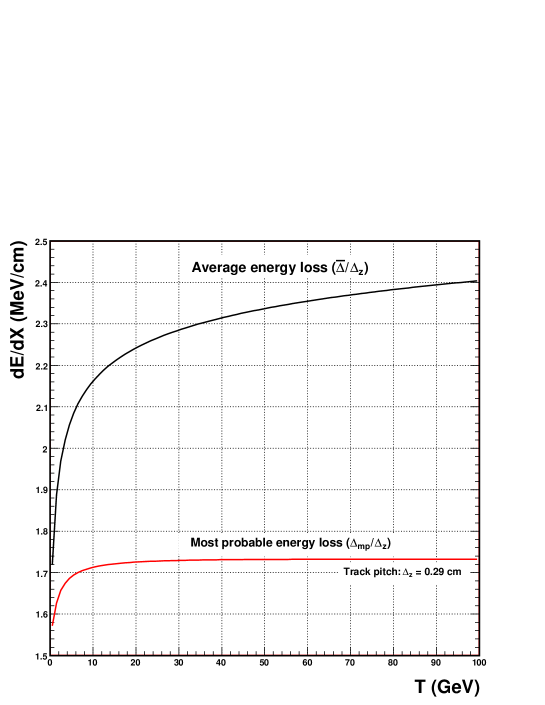
In order to measure the charge attenuation effect due to the LAr impurities, we analyze the dependence of as a function of the drift coordinate The procedure is as follows:
-
•
A histogram of every muon is obtained.
-
•
Every histogram is fitted to a convoluted Landau-Gaussian distribution, in order to obtain the most probable value of the distribution (). On the other hand, the average drift coordinate () of the track is computed as well.
-
•
A two dimensional distribution of the versus the mean drift time is built.
-
•
Finally, the latter distribution is converted into the profile form of Fig. 5.10 and then, fitted to a straight line.
From the slope of the curve in Fig. 5.10 is possible to obtain an accurate estimation of the electron drift lifetime during the data taking stage. When the drift time is much smaller than , the exponential attenuation of the drifting charge (Eq. (3.1)) can be approximated by an straight line, being the slope the inverse of the lifetime. Thus, from the fitted data in Fig. 5.10 we have a value for the slope of , which leads to a lifetime of with a relative error of %. Such a big error comes from the flatness of . This means that we are over the sensitivity limit of the measurement and that the attenuation over the drift distance is negligible.
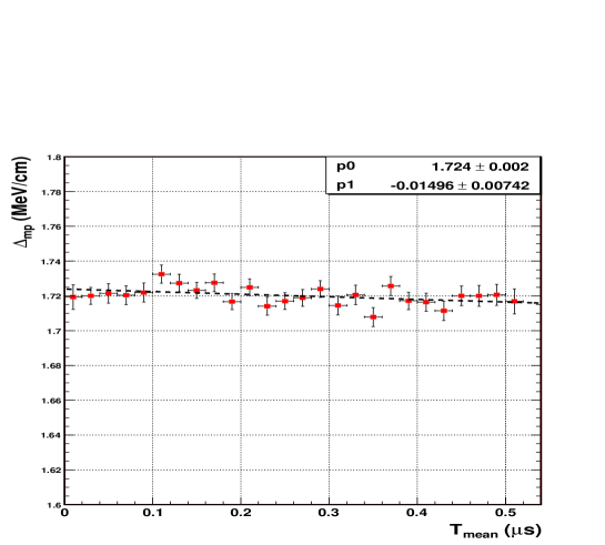
5.2.3 Beam alignment
In order to obtain a correct reconstruction of the events is mandatory to determine precisely the position of the chamber with respect to the beam. The alignment has been done moving the local reference system (RS) of the TPC (see Sec. 4.5.1) to the NOMAD reference system and then, to the beam. Since NOMAD alignment with respect to the beam was very precisely measured, this error source is less important than the one we will have for the alignment of the TPC with respect to NOMAD.
We call the rotation in the plane and the rotation in the plane. In terms of these angles, the alignment of NOMAD with respect to the beam is written as [92]
| (5.5) |
Alignment of the TPC respect to NOMAD
In order to determine the alignment parameters of the 50L TPC respect to the NOMAD RS, we made use of the same mip sample of Sec. 5.2.1 used for the electron drift velocity determination. There are 268 through-going muons correctly measured and reconstructed both by NOMAD and the LAr TPC. The relative angles and are then calculated through the minimization of the difference between the direction angles measured by the 50L and NOMAD respectively. Final distributions after the minimization are shown in Fig. 5.11. The value of the alignment parameters are determined as the ones which make these distributions to be centered at zero:
| (5.6) |
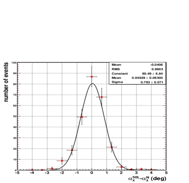 |
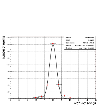 |
5.2.4 Energy calibration
As it was discussed in Sec. 4.6.5, the energy calibration consists in expressing the charge associated to a hit in energy units. The measured charge is related to the real deposited energy by means of a unit conversion constant () and the recombination factor ( in Eq. (4.30)). In this section, we measure the energy calibration factors for the 50L TPC under the assumption that the recombination factor is well described by Birk’s law in Eq. (4.31).
The overall calibration factor
The calibration factor converts the detector measuring units (ADC counts) into charge units (fC), and is usually obtained from a set of dedicated test pulses, simulating signals ranging from single to several tens of minimum ionizing particles [103, 74]. It was determined for the collection wires during the set-up phase before the data taking, when read-out was running in “charge” mode. As it was commented in Sec. 3.4, the final (and optimal) configuration adopted for the read-out worked in “current” mode which, unfortunately, did not have a calibration test pulse to measure .
Due to this lack of information, what we measure instead is the so called overall calibration factor in Eq. (4.30). To this purpose, we have collected a sample of around 3000 through-going muons coming from CC interactions. The spatial and calorimetric reconstruction of those muons allows to measure precisely the deposited charge per unit of length () as described in Sec. 4.6. We show in Fig. 5.12 the measured distribution of for the 3000 mouns in the sample: The data is fitted to a convoluted Landau-Gaussian function to obtain the most probable energy loss for mips in terms of detector charge units: ADC/cm.222The bar in means the value is given in detector charge units. The most probable energy loss slightly depends on the energy for the range of the muons being considered (see Fig. 5.9). From this measurement, can be obtained assuming that according to the theoretical prediction for muons in the range of energies of the beam, the most probable energy loss is MeV/cm, therefore:
| (5.7) |
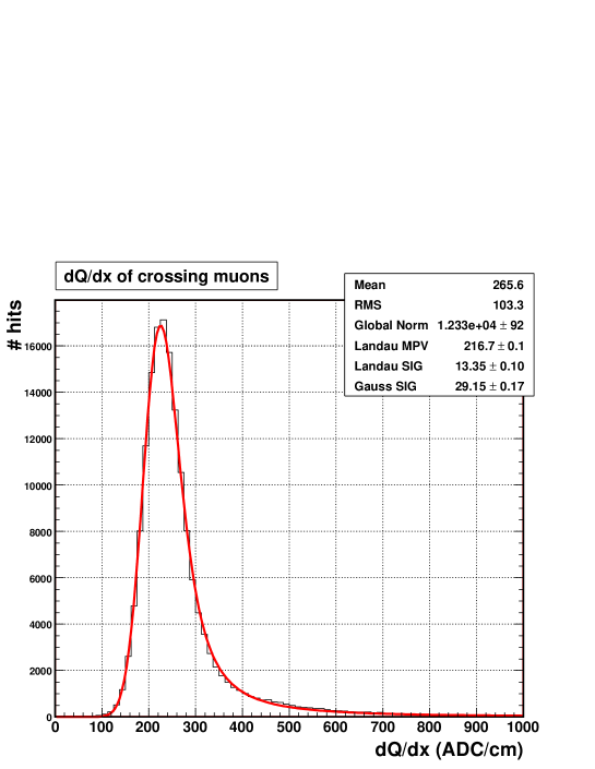
The recombination factor
As we discussed in Sec. 4.6.5, the recombination factor of drifting electrons strongly depends on the ionization density and this dependence of with can be modeled by Birk’s law (Eq. (4.31)):
The size of the range of the fully contained protons collected in the golden sample considered in Sec. 5.3, offers the opportunity to precisely test the energy loss pattern in the active medium. Fig. 5.13 shows the observed charge per unit length () versus the residual range for protons333The residual range is the actual range minus the range already covered at the time of the deposition of a given .. Dots are direct measurements from the reconstructed hits of the proton tracks. From this distribution we estimate the most probable value of for each bin of the residual range. Finally, from this data we fit cm/MeV ((4.31)) for the proton hypothesis (continuous line), constraining the value of to make compatible with Eq. (5.7) at mip region:
| (5.8) |
Based on the knowledge of the Birk’s law parameters, a precise determination of the deposited energy can be obtained through direct charge measurements by means of Eq. (4.31). Moreover, pure Bethe-Bloch ionization loss can be corrected by the detector response in the region of high , where quenching effects are more sizable. This correction is important for particle identification in LAr, which exploits the different energy loss of particles near the stopping point.
In summary, we have precisely measured all the calibration parameters needed for a proper kinematical reconstruction of the events occurring in the TPC. The electron drift velocity allows to translate time samples into the vertical coordinate , and the electron lifetime is needed to correct the attenuation of the measured charge. The alignment angles are very important to properly describe the kinematics on the transverse plane respect to the beam direction. Finally, the recombination factor precisely describes the calorimetric picture of the events. In Tab. 5.2, we summarize the measured values of the calibration parameters for the 50L detector.
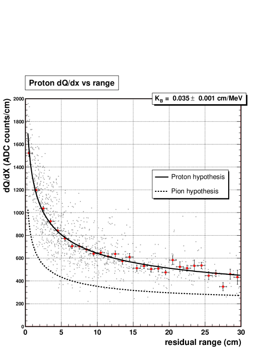
| Drift velocity | mm/s |
|---|---|
| Electron lifetime | ms (over the sensitivity limit) |
| Alignment angles | |
| MeV/ADC | |
| cm/MeV |
5.3 Analysis of quasi-elastic charge current interactions
5.3.1 Data taking and event selection
The data set recorded with the 50L chamber amounts to protons on target. As mentioned in Sec. 5.1, the trigger efficiency was monitored during data taking and its integrated value is 97%. Additional losses of statistics are due to the TPC (3%) and NOMAD (15%) dead time and to detector faults. These contributions add up to give an effective lifetime of 75%. Over the whole data taking period around 70000 triggers were collected in the TPC from which 20000 have at least a reconstructed muon possibly transversing the fiducial volume (see Sec. 5.3.3). From all these a priory CC candidates, a visual scanning reveals that around half of them show a vertex in the fiducial volume, the rest are interactions in the surrounding LAr bath (which also give trigger) plus a contamination of crossing muons due to veto inefficiencies. Therefore, we have a set of around 10000 CC events.
The golden sample
From the whole sample of CC events, we have selected a set of 86 events called the golden sample . They are events having a clear two prong topology with a mip leaving the chamber in the beam direction and an identified contained proton. The main features of the golden sample are the following:
-
•
An identified proton of kinetic energy larger than 40 MeV, fully contained in the TPC and one muon whose direction extrapolated from NOMAD matches the outgoing track in the TPC (see Sec.5.3.3).
-
•
The distance of the primary interaction vertex to any of the TPC walls has to be greater than 1 cm.
-
•
The muon candidate track projected onto the wire plane must be longer than 12 wire pitches.
-
•
The presence of other stopping particles is allowed as far as their visible range does not exceed the range of a proton of 40 MeV kinetic energy.
-
•
No other tracks than the identified muon can leave the TPC.
-
•
Events with at least one converted photon with an energy deposition in the fiducial volume greater than 10 MeV are also rejected.
The tightness of these selections makes the golden sample a very clean topology for visual scanning (Fig. 5.14 (Top)).
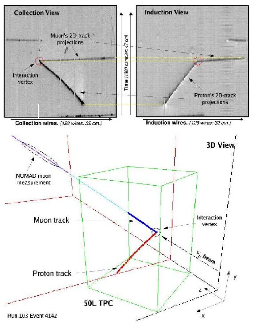
The request of containment is very severe since the chamber volume is small. On the other hand, for a kinetic energy () below 40 MeV the proton range is comparable with the wire pitch and neither the proton momentum nor the interaction vertex can be reconstructed with due precision. However, for MeV the /p misidentification probability is negligible (see Sec. 5.3.2).
5.3.2 Proton reconstruction
Proton identification and momentum measurement were performed using only the information provided by the TPC, following the reconstruction method explained in detail in Chap. 4.
Proton identification
In Sec. 4.6.4, we discussed that the average energy loss is a function of the mass and the kinetic energy of the particle. For the case of particles stopping in the fiducial volume of the chamber, a direct relation between their kinetic energy and their covered range (i.e. the distance a particle can penetrate before it loses all its energy) is obtained by means of the integration of Eq. (4.19) along the particle’s path (see Sec. 4.6.6).
The discrimination between protons and charged pions is performed exploiting their different energy loss behavior as a function of the range. For the case of candidates stopping in the fiducial volume of the chamber, as the ones of the golden sample , p/ separation is unique (see Fig. 5.15): is measured along the proton candidate track and is compared with the different particle hypothesis. Monte-Carlo studies reveal that almost 100% of protons are identified as such, on the basis of their shape on the vicinity of the stopping point; in addition, the fraction of pions and kaons misidentified as protons is negligible, showing thus the superb particle identification capabilities of the Liquid Argon TPC technique.
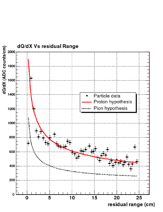
Momentum measurement
Once we identify a contained proton, its kinetic energy is calculated from range, which only depends on the spatial reconstruction of the tracks (see Sec. 4.6.6). In this case, the momentum uncertainty is dominated by the finite pitch of the wires (2.54 mm)444The equivalent pitch in the vertical direction (drift direction) is much smaller due to the high sampling rate of the fast ADC (m). and the performance of the reconstruction tools. For an uncertainty of wire in the determination of the starting and ending points of the projection of the track in both wire planes, and neglecting the error in the drift coordinate, a rough estimation of the error in the total length of the track is given by:
| (5.9) |
being the projection of the track in the collection/induction plane and the total track length. The error in the range determination is automatically translated into an error in the energy measurement. This has been tested using a Monte-Carlo simulation of the detector: The resolution on the kinetic energy () varies from 3.3% for protons with MeV up to 1% for larger than 200 MeV.
The angular resolution in the collection or induction view depends on the number of wires hit by the particle along its path; it is
| (5.10) |
which for a proton covering 10 wires () means an error of 15 mrad.
5.3.3 Muon reconstruction
As mentioned in Sec. 5.1, the modest size of the 50L TPC made necessary the use of NOMAD as an external muon spectrometer in order to be able to measure the prong muons produced in CC interactions. The kinematic reconstruction of the outgoing muons exploits the tracking capability of the NOMAD drift chambers (see Sec. 5.1.2). An event triggering the chamber will have at least one penetrating track reaching the T1 and T2 trigger scintillators bracketing the TRD of NOMAD (Sec. 5.1.3). The corresponding track, nearly horizontal at the entrance of the NOMAD drift chamber volume, is reconstructed with an average momentum precision given by Eq. (5.2) in Sec. 5.1.2. A 10 GeV horizontal muon crossing all the chambers ( m) is reconstructed with a precision of 2.2%.
Muon matching
The reconstructed particle is traced back to the TPC accounting for the magnetic field and the presence of the forward NOMAD calorimeter (Sec. 5.1.2). The latter introduces an additional - in fact, dominant - source of uncertainty due to multiple scattering (MS) in the iron plates of the forward calorimeter (see Sec. 5.1.2). For small scattering angles ( rad), the MS uncertainty on the transverse momentum is independent of and it turns out to be MeV. The correctness of the back-tracing procedure has been cross checked comparing the direction angles of the particles belonging to the mip sample, as measured by the TPC, with the corresponding quantity from NOMAD555Due to the high sampling rate of the TPC, the angular resolution in the plane, i.e. in the vertical plane along the nominal beam direction (-axis), is dominated by the NOMAD uncertainty..
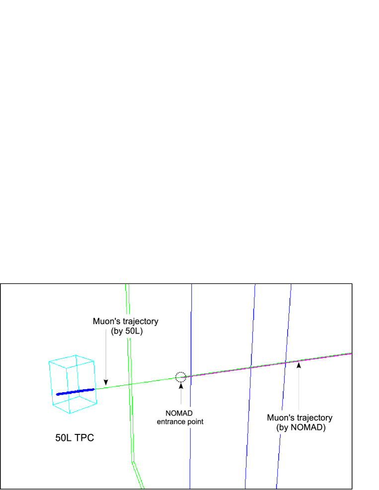
In Fig. 5.16 we show an example of the measurement of a single muon: the traced-back muon predicted from the NOMAD measurement is shown in pink, while the trajectory of the same muon extrapolated from the TPC data (blue points) is drawn in green. Both measurements are compared to each other at the same position located at the entrance of the NOMAD detector, in order to assure that the NOMAD muon is the same that traversed the TPC: Taking into account the errors in both measurements, we require that the difference between the traced-back muon and the original one is lower than 10 cm at NOMAD entrance point and their difference in angle below 100 mrad. As we comment in Sec. 5.3.4, the Monte-Carlo simulation reproduces both 50L and NOMAD measurements and thus, it allows to test the efficiency of the latter cuts, showing that more than of the muons fullfil those conditions (Fig. 5.17), being the rest low-energy muons strongly affected by multiple scattering in the front calorimeter.
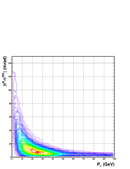
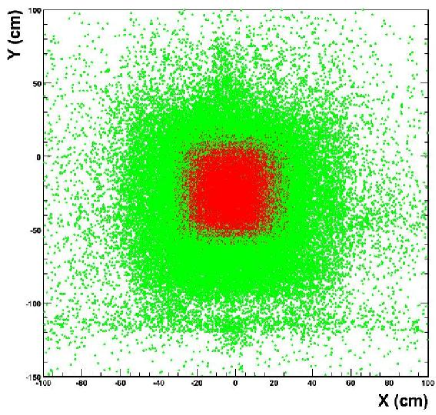
The kinematic reconstruction of the outgoing muon from NOMAD allowed us to identify the events produced outside the fiducial volume that trigger the chamber: The vast majority are interactions in the dewar or in the thermal bath plus a contamination of crossing muons due to veto inefficiencies. In Fig. 5.18 we show the distribution of the entrance point for all the triggering muons measured in NOMAD (in green) and just the ones which possibly transversed the active volume of the TPC (in red), which amount up to of the whole sample of triggering muons. As we commented at the beginning of Sec. 5.3.1, around half of them were effectively originated in interactions inside the chamber.
5.3.4 The Monte-Carlo data sample
Geometrical acceptance, background subtraction and QE selection efficiencies have been evaluated using a Monte-Carlo simulation. Neutrino-nucleus interactions are generated using NUX [104]. We use FLUKA [105] to simulate nuclear effects. NUX-FLUKA has successfully reproduced NOMAD data and therefore it is a reliable tool for the study of neutrino-nucleus interactions [106]. 100000 CC QE and non-QE events have been generated simulating the WANF beam for the 50L chamber geometrical acceptance (see Fig. 5.4) and final prompt particles emerging from neutrino-nucleus interactions are tracked through the 50 liter TPC and the NOMAD detectors by means of a GEANT4 simulation [107]. In Fig. 5.1 we show an output of a quasi-elastic CC event: The leading proton is fully contained within the TPC, while the prong muon goes out the TPC, passing through the front calorimeter, entering in the magnet with the drift chambers and finally giving a trigger in the scintillators planes. In order to efficiently reproduce the geometrical acceptance, the geometry and materials of the different sub-detectors have been simulated with care, using the detailed technical information presented in Sec. 5.1. The energy deposition of all final particles is digitized emulating the TPC wire read-out, in order to reproduce detector resolutions and offline reconstruction efficiencies.
Thanks to the simulation, full information about the final state particles and their energy deposition in LAr is provided. This information can be accessed both at particle level and at hit level, and besides, detailed information of secondary interactions is also available. Outside the TPC the simulation just take care of the trajectory of the muon, keeping the incoming position and momentum before the front calorimeter and immediately after, when the first of the drift chamber is hit. Finally, the impact position (if any) of the muon in the scintillator planes is recorded in order to decide if it gives trigger. The momentum measurement by NOMAD is also simulated and tracked-back to the LAr chamber taking into account multiple scattering effects in the front calorimeter (see Sec. 5.3.3).
To exemplify the results of the simulation and reconstruction tools, we show in Fig. 5.19 the visible energy (left) and the transverse missed momentum (right) of the golden sample compared to the Monte-Carlo expectation. We see that the resolution on the energy measurement is rather accurate given the good precision measurement that both the TPC and NOMAD can achieve for the proton and the muon energy respectively. About the kinematical reconstruction in transverse plane, the missed momentum is utterly dominated by the muon reconstruction, since it is affected by the presence of the front calorimeter (Sec. 5.3.3). On the other hand, the momentum direction of fully contained protons are very accurately measured thanks to the excellent 3D reconstruction capabilities of the LAr TPC.
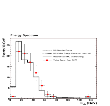 |
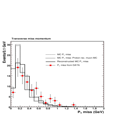 |
5.3.5 Geometrical acceptance
Due to the large amount of material between the TPC and the NOMAD trackers (more than 11 interaction lengths), there is an important fraction of discarded events: The prong muons leaving the chamber after a CC interaction can be stopped or deflected by the front calorimeter giving as a result a non-triggered or a bad-matched event. Obviously, the latter affects essentially to low energy and large angle muons. Neither the energy loss nor the multiple scattering in the front calorimeter are enough to disturb more energetic muons. The latter effect is shown in Fig. 5.20 (right) where we plot the geometrical acceptance as a function of the muon momentum for QE and DIS events separately.
In pure QE interactions, the fraction of the incoming neutrino momentum carried by the prong muon is nearly equal to due to the low energy transferred to the nucleon. Thus, the muon spectra slightly differs from the spectra of interacting neutrinos, which peaks around GeV (Fig. 5.20 (left)). On the contrary, non-QE (DIS RES) interactions are characterized by a high momentum transfer with the nucleus, which gives as a result a muon spectra shifted to low momentum values (Fig. 5.20 (left)). The convolution of the muon momentum distributions with their respective geometrical acceptance leads to a very significant difference between the total acceptance for QE events (96%) and non-QE events (72%).
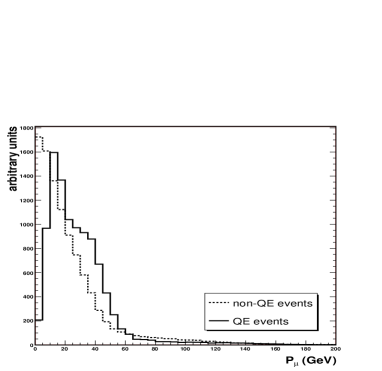 |
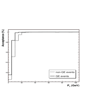 |
5.3.6 Background estimation
The golden sample contains pure QE interactions () plus an intrinsic background dominated by resonant production followed by pion absorption in the nucleus (). There is also an instrumental background due to resonance (RES) and deep-inelastic (DIS) events where final state neutral particles (’s, ’s and ’s) scape undetected. On the other hand, the contamination is negligible in this tightly selected sample due to the superb /p identification capabilities of the LAr TPC.
Thanks to the Monte-Carlo information we can properly simulate the selection cuts imposed to the golden events (see Sec. 5.3.1) over the full sample of generated events. Imposing such selection criteria, an algorithm efficiently selects the golden events from the whole sample of simulated QE interactions. We found that 16.6 % of them are golden, the rest are events with more particles in the final state due to nuclear re-interactions or having a not contained proton.666The automatic selection efficiency was cross-checked by means of visual scanning in a smaller sample of simulated data.
On the other hand, we have analyzed the sample of CC deep-inelastic (DIS) and resonant (RES) events in order to evaluate inefficiencies of the vetoing selections for (i.e. the probability to miss both the decay photons of the or the system in case of Dalitz decay) and for events with several neutral particles (neutrons and energetic photons from nuclear interactions) which scape from the detector (see Fig. 5.21). The search for this irreducible background in the DIS plus RES samples reveals that 0.14% are golden-like events.
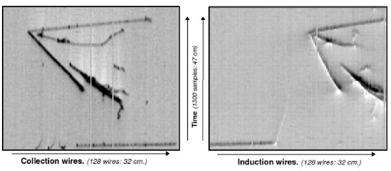
Taking into account the relative weight between QE and non-QE events777Respect to the total number of CC events, in our simulations, 2.3% are QE, 91.5% are DIS and the remaining 6.2% corresponds to RES events. The simulation of the latest is not done treating each resonance individually, an average of them is taken into account instead., we find that the total expected contamination of the golden sample is 28% (around 40% of them correspond to events with an escaping ). In Table 5.3, we summarize the parameters used in background estimation.
The Monte-Carlo prediction for escaping can be checked using test samples that consist of golden events with one () or two () converted photons pointing to the interaction vertex. Assuming the gamma identification probability to be uncorrelated for the two photons, we have and , being the (unknown) overall rate of final states and the photon identification efficiency. After the scanning of the test samples, turned out to be (43 9) %. Hence, the probability of missing both gammas is (3210) % to be compared with the MC calculation of 20.4%.
The estimated background is of utmost importance in the analyses of QE interactions being presented. It is key for a proper estimation the QE cross section calculation (Sec. 5.4). Furthermore, as we will discuss in Sec. 5.3.8, adding this sizable background leads to a much better description of the event kinematics.
| QE | non-QE | |
|---|---|---|
| Relative weight | % | % |
| Geom. acceptance | % | % |
| Golden fraction | % | % |
5.3.7 Event rates
We use Monte-Carlo to estimate the expected number of events in the detector. The simulation of the beam predicts a flux of //p.o.t. over the TPC exposing area. This flux convoluted with the neutrino cross sections and scaled to the fiducial mass of the detector (65.3 Kg of LAr) gives an event rate of CC/p.o.t. Now assuming a total exposure of p.o.t. and an effective lifetime of 75% (see Sec. 5.3.1), the total number of CC is equal to 18450. Out of these 18450 events, only muons above a certain momentum threshold and within angular acceptance will trigger the detector. The latter parameters for the experimental configuration are summarized in Table 5.4. Taking the real data muons that triggered the system, we saw that most of them are above 8 GeV in momentum and below 300 mrad in angle. If we apply those cuts to the Monte-Carlo samples, we end up with 18450 0.023 (QE fraction) 0.96 (efficiency of the acceptance cuts for QE), equal to 400 quasi-elastic events. For DIS+RES events: 18450 0.977 (fraction of DIS+RES) 0.72 (efficiency of acceptance cuts) gives 12600. In total we expect 13000 events to be compared with the 10000 CC we have after visual scanning of good triggers (see Sec. 5.3.1).
The expected number of golden events is obtained taking the 16.6% (golden fraction) of the total QE, and adding the corresponding 28% due to background contribution (see Sec. 5.3.6), which finally gives golden events to be compared with the 86 we observe. The systematic uncertainty is dominated by the fraction of QE events (2.3%) and the beam simulation (8%) 888A detailed discussion about the different sources of systematic errors can be found in Sec. 5.4, where the CC QE cross section is calculated..
| Neutrino Flux | //p.o.t. | |
|---|---|---|
| Interaction rate | CC/p.o.t. | |
| Total exposure | p.o.t. | |
| Effective detector lifetime | % |
5.3.8 Analysis of the kinematics of quasi-elastic interactions
In spite of the limited statistics (86 events), the golden sample provides information on the basic mechanisms that modify the kinematics of neutrino-nucleus interactions with respect to the corresponding neutrino-nucleon process. Nuclear matter perturbs the initial state of the interaction through Fermi motion; it also affects the formation of the asymptotic states through nuclear evaporation, hadronic re-scattering or hadronic re-absorption. Several kinematic variables are only marginally affected by nuclear effects; in this case, the corresponding distributions can be reproduced once the -nucleon interaction is corrected for Fermi motion and Pauli blocking. Clearly, purely leptonic variables belong to this category. There are also a few hadronic variables whose distribution is strongly influenced by the selection cuts but show limited sensitivity to nuclear effects. In particular, the proton kinetic energy is bounded by the MeV cut and the requirement of full containment in the fiducial volume. This distribution is shown in Fig. 5.22 together with the transverse momentum of the proton for the golden sample. Similarly, in Fig. 5.23 we show the kinetic energy and the transverse momentum distributions of the muon. Figs. 5.22 and 5.23 can be used as a consistency check. They demonstrate that Monte-Carlo reproduces the kinematic selection performed during the scanning and analysis of the golden channel. They also show that our selected sample contains a non-negligible contamination from non-QE events. As already indicated, we estimate this contamination to be 28 %.
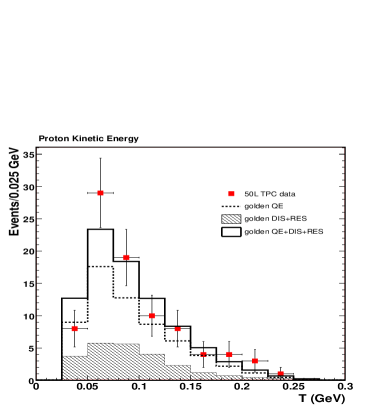 |
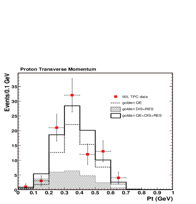 |
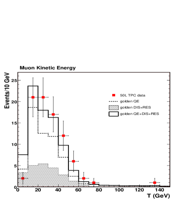 |
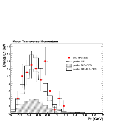 |
Other variables embedding the reconstructed kinematics of the protons are sensitive to genuine nuclear effects. In particular, we analyzed two of them: the acollinearity and the missing transverse momentum of the event. The former is defined as
| (5.11) |
and being the transverse momentum components of the proton and and the corresponding quantities for the muon. For a purely QE scattering on a nucleon, the muon and the proton ought to be back-to back in the transverse plane so that the acollinearity is zero. Fig. 5.24 (right) shows the acollinearity distribution for the golden sample and the expectation from simulations. For this particular variable, the inclusion of nuclear effects in the Monte-Carlo does not show a striking difference with respect to the case where no nuclear effects are taken into account. The selection cuts (in particular, the fact that the proton should be fully contained), the resolution NOMAD has for muon reconstruction and the contamination from non-QE events are the main reasons for the appearance of events with large acollinearity values. The distortion introduced in the tail of the acollinearity distribution by nuclear effects is much smaller than the one due to detector effects. Hence this variable is not adequate to show how the event kinematics varies in the presence of nuclear matter.
The influence of nuclear effects on the event kinematics is best seen when we consider the missing transverse momentum (see left plot on Fig. 5.24). We observe that a naive approach that takes into account Fermi motion and Pauli blocking disregarding nuclear effects (dashed histograms in Fig. 5.24 left) does not reproduce the data. Once nuclear effects are added, simulated events show a good agreement with data. The effect of background events is also relevant. Being the non-QE events more unbalanced than QE events in the transverse plane, they have the effect of shifting the expected theoretical distributions to higher values of , just like data do.
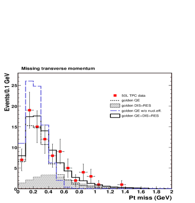 |
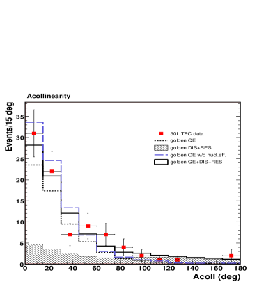 |
In order to quantify the level of agreement between the theoretical expectations and the data, we have performed a Kolmogorov test [75, 108] for some of the transverse variables. Such a test is based on a comparison between the cumulative distributions of the samples being analyzed (see Fig. 5.25, where cumulative distributions for and the acollinearity are shown). Its goal is to give a statistical estimation about how compatible is the data sample with being a random sampling from a given theoretical distribution. In Tab. 5.5 we quote the results of such a test in terms of the Kolmogorov probability. There, we test experimental data against three theoretical approaches: golden QE with no nuclear effects, golden QE with nuclear effects included and, finally, against golden QE plus the corresponding DIS and RES background999Theoretical distributions are always normalized to the golden sample data.. Clearly, nuclear effects offer a much better description of data than naive approaches commented above, mainly for the case of (see Tab. 5.5). On the other hand, the effect of adding the background leads to a better modeling of the missing transverse momentum and the acollinearity.
| Variable | Kolmogorov probability | ||
|---|---|---|---|
| QE w/o nucl. eff. | QE with nucl. eff | QE+DIS+RES with nucl. eff. | |
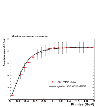 |
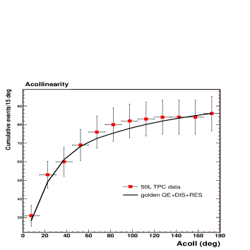 |
In summary, we have seen that nuclear effects are an important source of perturbation for the kinematics of quasi-elastic neutrino interactions, however the smallness of the accumulated statistics does not allow a systematic survey of these effects [109, 110]. Still, these results empirically demonstrate the effectiveness of LAr imaging in the characterization of low-multiplicity multi-GeV neutrino interactions [2]. In particular, as we discuss in Chap. 6, a good description of transverse variables is fundamental since they are key to a kinematic-based approach for oscillation appearance [4].
5.4 Measurement of the quasi-elastic CC cross section
The collected sample of golden events gives us the opportunity of measuring for first time the quasi-elastic CC cross section using a LAr TPC. To this purpose a precise knowledge of the beam composition, the beam profile, the exposition time, trigger efficiencies, acceptance cuts, event selection rates and background ratios is needed. In previous sections most of the required quantities have been already obtained, specially in Sec. 5.3.7 where an estimation of the expected number of QE events was discussed. In fact, the calculation of the cross section is like inverting the process we followed there, i.e. given the total number of measured golden events extract the quasi-elastic cross section. However, in order to give a competitive measurement instead of just a cross-check, a careful treatment of systematic errors has been done.
Event counting
As we wrote in Sec. 5.3.1, the total number of golden events collected is events. The data taking period corresponds to a total exposure protons on target, which must be corrected by the effective lifetime of the detectors (see Sec. 5.3.7). The events contained in the golden sample are pure QE interactions () plus an intrinsic and instrumental background (see Sec. 5.3.6). To compute the QE cross section, this background must be clearly understood and removed.
Background subtraction
The golden sample is contaminated with a sizable fraction of deep-inelastic (DIS) and resonance (RES) events. To estimate this contamination, we use
| (5.12) |
() is the number of true QE (non-QE) events inside the golden sample (). stands for the fraction of a given event class (i.e., in our Monte-Carlo, QE events amount to of the total. For non-QE events ). () is the acceptance for QE (non-QE) events and according to our simulations their average values are and . Finally, measures the fraction of events of a given class that are classified as golden. For QE events, we obtain . The fraction of non-QE events classified as golden is . Despite the smallness of this number, the final contamination in our golden sample is not negligible since, at these high energies, the majority of collected events are of non-QE nature. In particular, given the reduced size of our detector, most of the background comes from undetected since, as computed in Sec. 5.3.6 the probability to miss the two photons is almost one third. We have estimated that the final contamination inside the golden sample due to non-QE events is .
The measurement
After background subtraction, the golden sample contains genuine QE events. The beam simulation predicts a neutrino flux of /cm2/p.o.t. Knowing the values for the effective detector lifetime and the total exposure, we compute the total cross sections using
| (5.13) |
where is the number of target neutrons contained in the fiducial volume. The figures used for the rest of the variables have been discussed above. Hence, for an average neutrino energy of 29.5 GeV, the total QE cross section amounts to
Although a wide-band beam has been used, the reduced statistics accumulated during the test, do not allow to obtain a set of total cross sections measurements for several incoming neutrino energies.
Evaluation of systematics
The systematic error associated to our measurement was evaluated exploiting the full Monte-Carlo simulation of the experimental set-up (Sec. 5.3.4). To better identify the different contributions to the systematic uncertainty, it is much more convenient to express Eq. (5.13), after a trivial change of variables, as:
| (5.14) |
We identify three types of systematic errors: The first one involves the knowledge of the experimental setup, the neutrino flux and the detector performance (see Sec. 5.1). The second is related to the golden event selection criteria (Sec. 5.3.1) and the geometrical acceptance (Sec. 5.3.5). Finally, we have the systematics associated with the determination of the fraction of golden events and the expected ratio between QE and non-QE events, which strongly depends on the modeling of neutrino-nucleus interactions (see Sec. 5.3.4) and the experimental uncertainties in the cross sections at these energies.
In the following, we summarize and describe in detail the different sources of systematics entering in the cross section calculation through Eq. (5.14):
- •
-
•
The uncertainty associated to the fiducial volume has been evaluated varying its dimensions by wire in the wire coordinate and drift samples on the time coordinate. The measured resolution on the time coordinate is much better, however we have adopted a conservative approach when evaluating this kind of systematic error. The discussed modification of the fiducial volume causes a variation on the number of golden events that amounts to . We take this value as the systematic error associated to the fiducial cut.
-
•
The criteria used for event selection are another source of systematics. The energy resolution for stopping hadrons is estimated to be about 4 and for converted photons we take . This translates into a final systematic error of due to the definition of a golden candidate.
-
•
The main source of systematics for the geometrical acceptance comes from the criteria used to match the reconstructed muons in NOMAD with the ones that exit the 50 liter LAr TPC (see Sec. 5.3.3). Due to the small lever-arm of the TPC, the resolution on the measurement of the muon direction is, on average, mrad. To evaluate how this uncertainty affects the muon acceptance, we have modified the matching criteria described above by mrad. The error on the geometrical acceptance turns out to be for QE and non-QE samples. These errors translate into a systematic contribution of () for QE (non-QE) events.
-
•
The fraction of golden events inside the QE and non-QE samples is affected by nuclear effects, which modify the topology and kinematics of the final state. Following the discussion in [111], where the acceptance for identification of QE CC events in a fine grained detector is studied as a function of the proton detection threshold and nuclear effects, we conservatively take that varies by due to uncertainties in the modeling of nuclear effects inside the Monte-Carlo. With this assumption, the systematic error on the cross section due to the fraction of golden events inside the QE sample amounts to 16. This is the dominant error source. A similar error on () contributes to on the total systematic.
-
•
Finally, the ratio of QE versus non-QE events is assumed to be known at the level of from experimental uncertanties in the cross section [112]. Its contribution to the cross section systematic error is .
Table 5.6 summarizes the contributions from the different systematic uncertainties.
All in all, the estimated total systematic error is . This translates onto a measurement of the total QE charged-current cross section:
| (5.15) |
This value agrees with previous measurements of this reaction reported in the literature (see Fig. 5.26 and references [113, 114, 115, 116, 117, 118, 119]), and it stands as the first Physics measurement ever done with a LAr TPC using a neutrino beam from an accelerator.
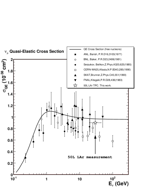
| Source | Systematic error (%) | |
| Neutrino flux | 8 | |
| Detector lifetime | 4 | |
| Vertex detection (fiducial cut) | 3 | |
| Golden event selection cuts | 6 | |
| Acceptance for QE events, | 1.5 | |
| Acceptance for non-QE events, | 0.5 | |
| Fraction of golden events in QE sample, () | 16 | |
| Fraction of golden events in non-QE sample, () | 5 | |
| Fraction of non-QE to QE events, () | 4 | |
| Total | 20.6 |
Chapter 6 Searching for oscillations at CNGS
The Super-Kamiokande Collaboration has measured a first evidence of the sinusoidal behaviour of neutrino disappearance as dictated by neutrino oscillations [120]. However, although the most favoured hypothesis for the observed disappearance is that of oscillations, no direct evidence for appearance exists up to date. A long baseline neutrino beam, optimized for the parameters favoured by atmospheric oscillations, has been approved and is now running in Europe to look for explicit appearance: the CERN-Laboratori Nazionali del Gran Sasso (CNGS) beam [121]. The approved experimental program consists of two experiments ICARUS [69] and OPERA [122] that will search for oscillations using complementary techniques.
Given the previous experimental efforts [92, 93] and present interest in direct appearance, we assess in this Chapter the performance of several statistical techniques applied to the search for using kinematic techniques. Classic statistical methods (like multi-dimensional likelihood and Fischer’s discriminant schemes) and Neural Networks based ones (like multi-layer perceptron and self-organized neural networks) have been applied in order to find the approach that offers the best sensitivity.
The underlying idea consists on finding the kinematical features which characterize the signal respect to the dominant background. To this purpose is obvious that optimal reconstruction capabilities are of utmost importance. In Chapter 5 we have assessed the excellent performance of our reconstruction tools when they are applied to the analysis of the kinematics of CC events. Furthermore, we have also seen that our Monte-Carlo accurately describes neutrino-nucleus interactions and nuclear effects. Thanks to these successfully tested capabilities, in this Chapter, we can use them to evaluate the performance of a LAr TPC when searching for direct appearance of at CNGS.
6.1 On the problem of appearance at CNGS
In the CERN-NGS beam [121, 123], the expected and contamination are of the order of and respectively compared with the dominant composition. These properties allow to search for oscillations by looking at the appearance of and charged current events. In these cases, the detector must be able to tag efficiently the interaction of ’s and ’s out of the bulk of events.
In the case of oscillations, the golden channel to look for the appearance is the decay of the tau into an electron and a pair neutrino anti-neutrino due to: (a) the excellent electron identification capabilities of a LAr TPC; (b) the low background level, since the intrinsic and charged current contamination of the beam is at the level of one per cent.
Kinematical identification of the decay, which follows the CC interaction, requires excellent detector performance: good calorimetric features together with tracking and topology reconstruction capabilities. In order to separate events from the background, two basic criteria can be used:
-
•
An unbalanced total transverse momentum due to neutrinos produced in the decay.
-
•
A kinematical isolation of hadronic prongs and missing momentum in the transverse plane.
6.1.1 Detector configuration and data simulation
As a reference for this study, we consider a detector configuration consisting of 5 identical T600 modules (T3000 detector) 111See Sec. 2.2 for a brief description of the ICARUS detector or consult Ref. [69] for a much more detailed description.. As the active Argon for one of these modules is 470 tons, the total mass amounts to 2.35 ktons. We also assume five years running of the CNGS beam in shared mode ( p.o.t. per year), which translates in a total exposure of Ktonyear.
Events have been fully simulated in the whole of each T600 module ( m3), but only have the primary interaction vertex inside the active part of the LAr volume.
The study of the capabilities to reconstruct high-energy neutrino events was done using fully simulated CC events inside the considered LAr detector [124]. The neutrino cross sections and the generation of neutrino interactions is based on the NUX code [104]; final state particles are then tracked using the FLUKA package [105]. The angular and energy resolutions used in the simulation of final state electrons and individual hadrons are identical to those quoted in [69]: equal to for hadrons and for electromagnetic showers ( in units of GeV). Concerning the reconstruction of the particle direction, the assumed angular resolutions are for electrons and for single hadrons. In the analyses, the particle four vectors are smeared according to the previous parameters.
The fiducial volume
The ability to look for tau appearance events is limited by the containment of high energy neutrino events. Energy leakage outside the active image volume creates tails in the kinematical variables that fake the presence of neutrinos in the final state. We therefore impose fiducial cuts in order to guarantee that on average the events will be sufficiently contained.
The fiducial volume is defined by looking at the profiles of the total missing transverse momentum and of the total visible energy of the events. The average value of these variables is a good estimator of how much energy is leaking on average.
The profiles of missing and visible energy as a function of the vertex positions for the T600 module are shown in Fig. 6.1. We have to leave 20 cm at the top and bottom of the active volume (x coordinate), and 25 cm from the sides (y coordinate). Longitudinally, we cut out 1.7 m from the total length (z coordinate). This results in a total fiducial volume of m3. Thus with this conservative approach, we keep 65% of the total number of events occurring in the active LAr volume. The total exposure in a 5 T600 setup with 5 years shared running CNGS, taking in account the fiducial cuts, is 7.6 ktonyear. In what follows, tau selection and background rejection efficiencies are normalized to this figure.

6.1.2 Expected rates and generated data
Tab. 6.1 summarizes the total event rates expected for 5 T600 modules and 5 years CNGS running. It also shows, for different values of , the expected CC rates in case oscillations take place.
| Expected events | Expected events | |
| Process | Active LAr. | Fiducial LAr. |
| (11.75 Ktonyear) | (7.6 Ktonyear) | |
| CC | 32600 | 21190 |
| CC | 652 | 424 |
| CC | 252 | 163 |
| CC | 17 | 11 |
| NC | 10600 | 6890 |
| NC | 245 | 159 |
| CC, (eV2) | ||
| 31 (6) | 20 (4) | |
| 125 (23) | 81 (15) | |
| 280 (50) | 182 (33) | |
| 750 (135) | 488 (88) |
The rate has a strong dependence on the exact value of the in the parameter region favoured by atmospheric data as we see in table 6.1. For our central value taken from atmospheric neutrino results (), the number of CC with is about 50; the signal over background ratio is .
Tab. 6.2 summarizes the total amount of simulated data. We note that CC sample, generated in active LAr, is more than a factor 250 (50) larger than the expected number of collected events after five years of CNGS running.
| Process | CC | CC |
|---|---|---|
| () | ||
| Total LAr | 22500 | 22100 |
| Active LAr | 14200 | 13900 |
| Fiducial Vol. | 9250 | 9000 |
To save CPU power, only CC events with an incoming neutrino energy below 30 GeV have been generated, since oscillated events, with a , tend to accumulate in the low energy region (only 3% of the total CC events have an energy above 30 GeV).
6.2 Statistical pattern recognition applied to oscillation searches
In the case of a oscillation search with Liquid Argon, the golden channel to look for appearance is the decay of the tau into an electron and a pair neutrino anti-neutrino due to: (a) the excellent electron identification capabilities; (b) the low background level, since the intrinsic and charged current contamination of the beam is at the level of one per cent.
Kinematic identification of the decay [125], which follows the CC interaction, requires excellent detector performance: good calorimetric features together with tracking and topology reconstruction capabilities. In order to separate events from the background, a basic criteria can be used: an unbalanced total transverse momentum due to neutrinos produced in the decay.
In Fig. 6.2 we illustrate the difference on kinematics for signal and background events. We plot four of the most discriminating variables:
-
•
: Visible energy.
-
•
: Missing momentum in the transverse plane with respect to the direction of the incident neutrino beam.
-
•
: Transverse momentum of the prompt electron candidate.
-
•
Signal events tend to accumulate in low , low , low and high regions.
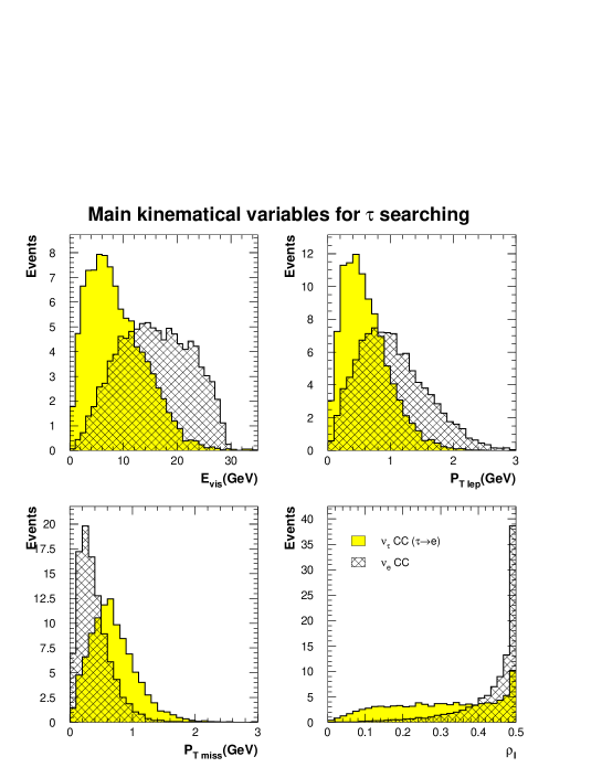
Throughout this work, we take into account only the background due to electron neutrino charged current interactions. Due to the low content the beam has on , charged currents interactions of this type have been observed to give a negligible contribution to the total expected background. We are confident that neutral current background can be reduced to a negligible level using LAr imaging capabilities and algorithms based on the different energy deposition showed by electrons and (see for example [126]). Therefore it will not be further considered. The contamination due to charm production and CC events, where the prompt muon is not identified as such, was studied by the ICARUS Collaboration [127] and showed to be less important than CC background.
6.2.1 Direct Background rejection using Sequential Cuts
The most straightforward way to look for appearance is by means of a series of sequential cuts. This procedure does not take into account possible correlations among the selected kinematical variables. We take advantage of the soft energy spectrum for oscillated induced events with respect to the visible energy spectrum of CC. Oscillated events tend to accumulate at relatively low values of , as well, therefore an upper cut on efficiently removes the background. Since CC events are well balanced and very few populate the high region (missing momentum in the plane perpendicular to the incoming neutrino direction), a cut in this variable is also applied.
Tab. 6.3 summarizes the list of sequential cuts applied to reduce the CC background. The expected number of signal events, for eV2, after all cuts is , for a total background of expected events222Errors in the number of expected events are of statistical nature. The usual Poisson statistical error in probability density estimation is rescaled according to the distribution normalization (5 years of CNGS running). . Fig. 6.3 shows some kinematical variables for signal and background events surviving the cuts. The signal to background ratio (S/B) for this approach is around five. More sophisticated techniques, taking into account correlations among discriminating variables, should be used in order to improve the S/B value.
| CC() | CC () | ||
| Cuts | Efficiency | CC | |
| () | eV2 | ||
| Initial | 100 | 252 | 50 |
| Fiducial volume | 64 | 161 | 32 |
| GeV | 62 | ||
| GeV | 51 | ||
| GeV | 43 | ||
| GeV | 23 |
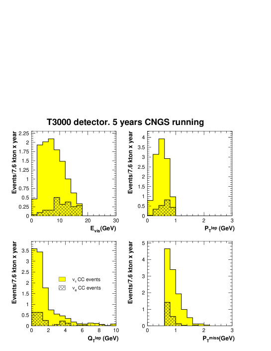
6.2.2 Kinematical search using classic statistical methods
A multi-dimensional likelihood
The second method adopted for the analysis is the construction of a multi-dimensional likelihood function (see for example [128]), which is used as the unique discriminant between signal and background. This approach is, a priori, an optimal discrimination tool since it takes into account correlations between the chosen variables.
A complete likelihood function should contain five variables (three providing information of the plane normal to the incident neutrino direction and two more providing longitudinal information). However, in a first approximation, we limit ourselves to the discrimination information provided by the three following variables: , and .
As we will see later, all the discrimination power is contained in these variables, therefore we can largely reduce the complexity of the problem without affecting the sensitivity of the search. Two likelihood functions were built, one for signal () and another for background events (). The discrimination was obtained by taking the ratio of the two likelihoods:
| (6.1) |
In order to avoid a bias in our estimation, half of the generated data was used to build the likelihood functions and the other half was used to evaluate overall efficiencies. Full details about the multi-dimensional likelihood algorithm can be found elsewhere [126]. However, we want to point out here some important features of the method.
A partition of the hyperspace of input variables is required: The multi-dimensional likelihood will be, in principle, defined over a lattice of bins. The number of bins to be filled when constructing likelihood tables grows like where is the number of bins per variable and the number of these variables. This leads to a “dimensionality” problem when we increment the number of variables, since the amount of data required to have a well defined value for ln in each bin of the lattice will grow exponentially.
In order to avoid regions populated with very few events, input variables must be redefined to have the signal uniformly distributed in the whole input hyperspace, hence , and are replaced by “flat” variables (see Fig. 6.4). In general, a variable defined as
| (6.2) |
is uniformly distributed (“flat”) between 0 and 1 by choosing , where is a variable distributed according to a p.d.f. . With this approach, more bins are automatically taken in those regions of faster variation of the signal. The combination of the “flat” variables into a single one did not give rise to an uniform three dimensional distribution, due to the presence of correlations between the variables.
Besides, an adequate smoothing algorithm is needed in order to alleviate fluctuations in the distributions in the hyperspace and also, to provide a continuous map from the input variables to the multi-dimensional likelihood one (ln).
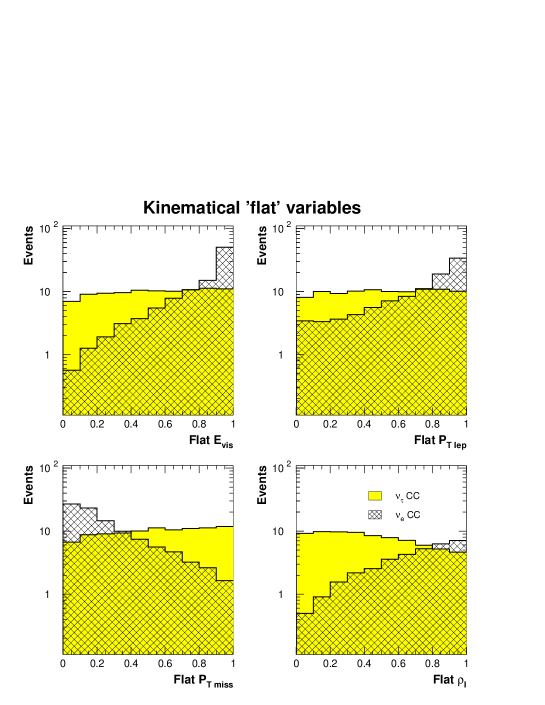
Ten bins per variable were used, giving rise to a total of bins. Fig. 6.5 shows the likelihood distributions for background and tau events assuming five years running of CNGS (total exposure of 7.6 kton year for events occurring inside the fiducial volume).
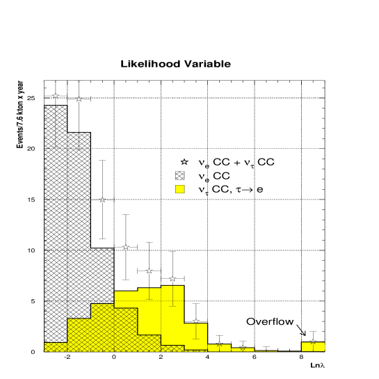
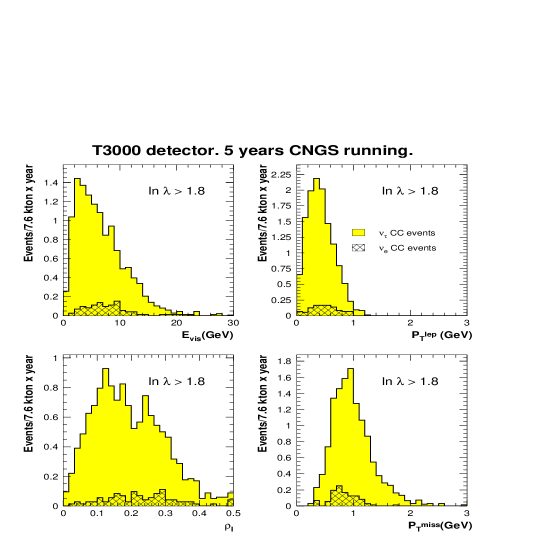
Tab. 6.4 shows, for different cuts of , the expected number of tau and CC background events. As reference for future comparisons, we focus our attention in the cut ln. It gives a signal selection efficiency around 25% (normalized to the total number of events in active LAr). This efficiency corresponds to 13 signal events. For this cut, we expect background events. After cuts are imposed, this approach predicts a S/B ratio similar to 13. The background rejection power is enhanced with respect to the sequential cuts, since correlations among variables are taken into account. In Fig. 6.6, we show the distribution of the surviving signal and background events for ln. The region selected by the multidimensional likelihood approach, in the three dimensional space of the chosen variables, does not present sharp edges like in the case of sequential cuts: The topology of the selected region is more complex thanks to the use of variable correlations.
| Cuts | CC | CC | |
|---|---|---|---|
| Efficiency | CC | ||
| () | eV2 | ||
| Initial | 100 | 252 | 50 |
| Fiducial volume | 65 | 164 | 33 |
| 48 | |||
| 42 | |||
| 36 | |||
| 30 | |||
| ln | 25 | ||
| ln | 23 | ||
| 16 | |||
| 10 | |||
| 7 |
The Fisher discriminant method
The Fisher discriminant method [128] is a standard statistical procedure that, starting from a large number of input variables, allows us to obtain a single variable that will efficiently distinguish among different hypotheses. Like in the likelihood method, the Fisher discriminant will contain all the discrimination information.
The Fisher approach tries to find a linear combination of the following kind
of an initial set of variables which maximizes
| (6.3) |
where is the mean of the variable and its variance. This last expression is nothing but a measurement, for the variable , of how well separated signal and background are. Thus, by maximizing Eq. (6.3) we find the optimal linear combination of initial variables that best discriminates signal from background. The parameters which maximize Eq. (6.3) can be obtained analytically by (see [128])
| (6.4) |
where and are the mean in the variable for signal and background respectively, and . , the covariance matrices for the two event classes considered, are defined as:
| (6.5) |
where k stands for signal or background classes, is a vector of data with means and N is the total number of events.
A Fisher function for search
From the distributions of kinematical variables for CC and CC, we can immediately construct the Fisher function for a given set of variables. Initially we selected the same set of variables we used for the likelihood approach, namely: , and . We need only the vector of means and covariance matrices in order to calculate the optimum Fisher variable (Eq. (6.4)). Distributions are shown in Fig. 6.7, where the usual normalization has been assumed. In Tab. 6.5 values for the expected number of signal and background events are shown as a function of the cut on the Fisher discriminant. Since correlations among variables are taken into account, it is not surprising that the result for the Fisher discriminant method is similar to the one obtained using a multidimensional likelihood.
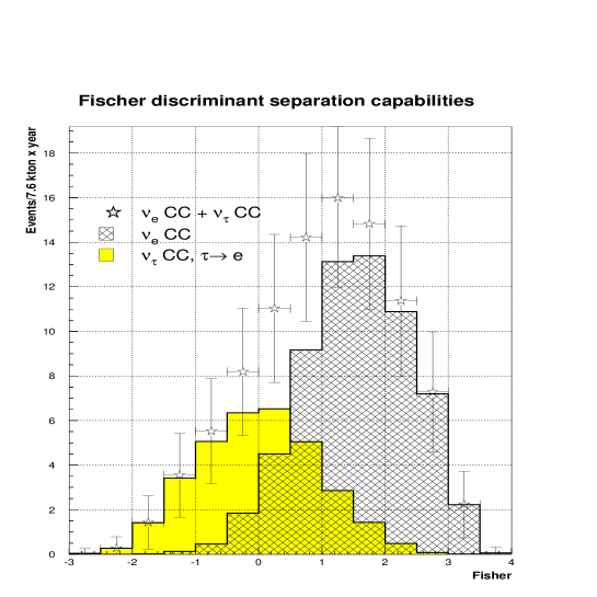
| Cuts | CC () | CC () | |
|---|---|---|---|
| Efficiency | CC | ||
| (%) | eV2 | ||
| Initial | 100 | 252 | 50 |
| Fiducial volume | 65 | 164 | 33 |
| Fisher | 46 | ||
| Fisher | 33 | ||
| Fisher | 25 | ||
| Fisher | 20 | ||
| Fisher | 10 |
Increasing the number of initial kinematical variables
Contrary to what happens with a multi-dimensional likelihood (where the increase in the number of discriminating variables demands more Monte-Carlo data and therefore it is an extreme CPU-consuming process), the application of the Fisher method to a larger number of kinematic variables is straightforward, since the main characteristic of the Fisher method is that the final discriminant can be obtained algebraically from the initial distributions of kinematic variables. For instance, a Fisher discriminant built out of 9 kinematic variables (, , , , , , , , )333see [125] for a detailed explanation of the variables predicts for taus a background of CC events. We conclude that, for the Fisher method, increasing the number of variables does not improve the discrimination power we got with the set , , and therefore these three variables are enough to perform an efficient appearance search.
6.2.3 Kinematical search using neural networks
In the context of signal vs background discrimination, neural networks arise as one of the most powerful tools. The crucial point that makes these algorithms so good is their ability to adapt themselves to the data by means of non-linear functions.
Artificial Neural Networks techniques have become a promising approach to many computational applications. It is a mature and well founded computational technique able to learn the natural behaviour of a given data set, in order to give future predictions or take decisions about the system that the data represent (see [81] and [129] for a complete introduction to neural networks). During the last decade, neural networks have been widely used to solve High Energy Physics problems (see [130] for a introduction to neural networks techniques and applications to HEP). Multilayer Perceptrons efficiently recognize signal features from, an a priori, dominant background environment ([131], [132]).
We have evaluated neural network performance when looking for oscillations. As in the case of a multidimensional likelihood, a single valued function will be the unique discriminant. This is obtained adjusting the free parameters of our neural network model by means of a training period. During this process, the neural network is taught to distinguish signal from background using a learning data sample.
Two different neural networks models have been studied: the multi-layer perceptron and the learning vector quantization self-organized network. In the following, their foundations and the results obtained with both methods are discussed.
The Multi-layer Perceptron
The multi-layer perceptron (MLP) function has a topology based on different layers of neurons which connect input variables (the variables that define the problem, also called feature variables) with the output unit (see Fig. 6.8). The value (or “state”) a neuron has, is a non-linear function of a weighted sum over the values of all neurons in the previous layer plus a constant called bias:
| (6.6) |
where is the value of the neuron in layer ; is the weight associated to the link between neuron in layer and neuron in the previous layer ; is a bias defined in each neuron and is a non-linear function called transfer function. The transfer function is used to regularize the neuron’s output to a bounded value between 0 and 1 (or -1,1). An usual choice for the transfer function is the sigmoid function (see Fig. 6.9),
| (6.7) |
This function tries to mimic the response of biological neurons by putting the neuron in a high () or low () state depending on the output of the previous neurons and how the links (weights) are set. The temperature parameter is not determinant in principle and is always set to 1.
These kind of structures for a Neural Network, where the information is propagated from the input units to the output ones passing through different ordered layers, are called feed forward neural networks.


Training the MLP
In a multi-layer perceptron a non-linear function is used to obtain the discriminating variable. The MLP is fed with a set of input variables which define the problem. The way the MLP sets its free parameters is through minimization of an error function. This error function is defined as:
| (6.8) |
where represents the MLP output for a given event belonging to the training sample, and is the “desired output”. The previous expression is nothing but a distance between the current MLP performance and the ideal case. In pattern recognition tasks, we would like to have some kind of discrimination function which, in an ideal case, always gives the correct answer, i.e., 1 for signal events and 0 for background events.
Once a topology is chosen for the MLP (number of layers and neurons per layer), we need a first sample of signal and background events for the training stage. The weights and the biases are then adapted, minimizing the error function (6.8), following the standard back-propagation algorithm (see [81] or [129]), which is the general procedure for a general feed-forward neural network and an arbitrary differentiable activation function. The process of adapting the parameters is repeated over the training sample during a number of “epochs” until some condition is fulfilled (usually when a stable minimum is reached).
At the end of the training stage, the network is made, and final weights and biases of the network are the ones which provide the best response for the training sample. In order to determine the real discrimination capabilities of the MLP, we need to test the neural network performance over an statistically independent sample (to avoid biases).
Freedom of choice
The construction of a MLP implies that several choices must be made a priori:
-
•
Number of input variables: The MLP can be fed, in principle, with as many variables as we consider fit in order to fully define our pattern recognition problem. We need to know a priori which variables (or combination of them) represent the main features of the classes in our pattern selection task. Redundant variables contribute to a worse performance of the MLP, hence is better to reduce the number of input variables to avoid a loss of discrimination power.
-
•
Number of hidden layers: It depends on the specific task one wants the network to perform, but a general statement is that no more than two hidden layers are needed. In pattern classification tasks, regions in input space must be created depending on the class they belongs. It could be shown (see [81]) that a MLP with no hidden layers only can made decision boundaries consisting in a hyperplane, one hidden layer can perform a single convex region consisting in hyperplanes segments, finally, two hidden layers could generate arbitrary decision regions. Hence, if your classes are very mixed in the variable space, two hidden layers will be able to construct more complex region borders.
-
•
Number of neurons per layer: The view of pattern classification as a “cut out” procedure gives a clue to the minimum number of hidden units needed for a specific classification task. In the “hard” case, where the first hidden layer has to define the border of a closed volume in the input space, at least (N+1) units (where N is the number of input variables) are needed. The second hidden layer usually performs some kind of logical function on the units belonging to the first hidden layer, therefore, a small number of neurons (1 or 2) is enough444Logical function as AND or OR can be exactly performed using a perceptron with no more than one hidden layer with two neurons. See [130] for an example..
-
•
Number of events in each sample: The size of the simulated data set is crucial in order to optimize the training algorithm performance. If the training sample is small, it is likely for the MLP to adjust itself extremely well to this particular data set, thus losing generalization power (when this occurs the MLP is over-learning the data). Over-learning can be tested on-line by defining a statistical independent sample to compute the error function in each step of the learning procedure.
-
•
Number of epochs: The number of iterations in the training procedure depends on how low and stable is the minimum we get. In addition over-learning must be avoided: by definition, the error curve in the learning sample is always macroscopically decreasing, however the error curve in test sample could start to rise. At this moment the MLP loses generalization power. Hence, we must stop our learning phase before over-learning starts.
Multi-layer Perceptron setup
As already mentioned in 6.2.2, five variables (three in the transverse plane and two in longitudinal direction) utterly describe the event kinematics, provided that we ignore the jet structure; therefore, using five independent variables we fully define our tagging problem. Initially we build a MLP that contains only three input variables, and in a latter step we incorporate more variables to see how the discrimination power varies. The three chosen variables are , and . Our election is similar to the one used for the multidimensional likelihood approach, this allows to make a direct comparison of the sensitivities provided by the two methods.

There are plenty of packages available on the market which implement a multi-layer perceptron. The simplest choice for us was to use the MLPfit package [133], interfaced in PAW.
We have opted for a neural network topology consisting on two hidden layers with four neurons in the first hidden layer and one in the second (see Fig. 6.10).
Simulated data was divided in three, statistically independent, subsets of 5000 events each (2500 signal events and a similar amount of background).
The MLP was trained with a first “training” data sample. Likewise, the second “test” data set was used as a training sample to check that over-learning does not occur. Once the MLP is set, the evaluation of final efficiencies is done using the third independent data sample (namely, a factor 40 (75) larger than what is expected for background (signal) after five years of CNGS running with a T3000 detector).
Error curves (Eq. (6.8)) during learning are shown in Fig. 6.11 for training and test samples. We see that even after 450 epochs, over-learning does not take place. Final distributions in the multi-layer perceptron discriminating variable can be seen in Fig. 6.12.

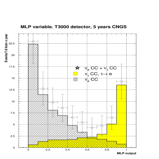
Results of MLP analysis
Fig. 6.13 shows the number of signal and background expected after 5 years of data taking as a function of the cut in the MLP variable. In Fig. 6.14 we represent the probability of an event, falling in a region of the input space characterized by MLP output cut to be a signal event (top plot), and the statistical significance as a function of the MLP cut (bottom plot). Like in the case of the likelihood, a cut based on the MLP output variable can select regions of complicated topology in the kinematical hyperspace (see Fig. 6.15).
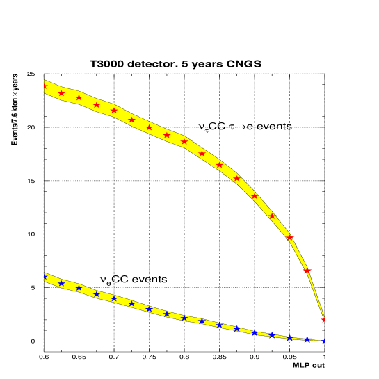
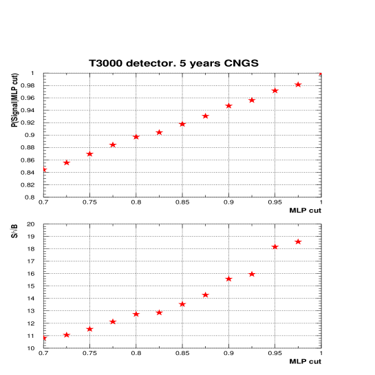
Selecting (overall selection efficiency %), the probability that an event falling in this region is signal amounts to . For 5 years of running CNGS and a T3000 detector, we expect a total amount of CC () events and CC events. Tab. 6.6 summarizes as a function of the applied MLP cut the expected number of signal and background events.
If we compare the outcome of this approach with the one obtained in section 6.2.2, we see that for the same selection efficiency, the multidimensional likelihood expects background events. Therefore, for this particular cut, the MLP achieves a 60% reduction in the number of expected CC background events.
| Cuts | CC () | CC () | |
|---|---|---|---|
| Efficiency | CC | ||
| (%) | eV2 | ||
| Initial | 100 | 252 | 50 |
| Fiducial volume | 65 | 164 | 33 |
| 42 | |||
| 40 | |||
| 37 | |||
| 33 | |||
| 27 | |||
| 25 | |||
| 19 | |||
| 12 |
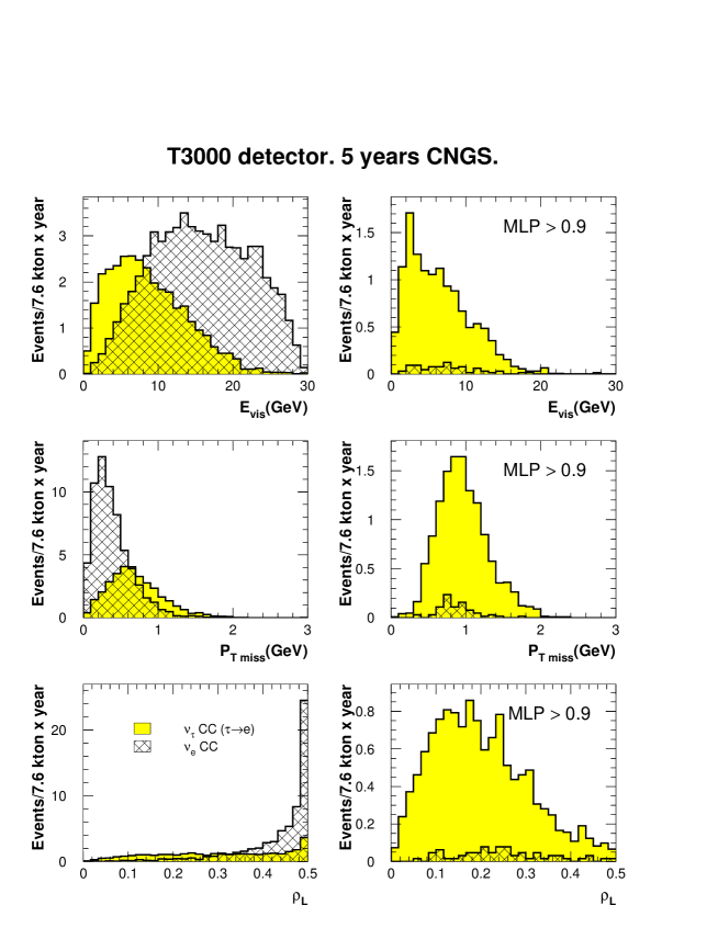
Increasing the number of feature variables
Contrary to the likelihood approach, where the lack of very large Monte-Carlo samples, increases the complexity of the problem as the number of input variables grows (even for three input variables, smoothing algorithms have to be applied in order to get smooth distributions throughout the hyper-space), the MLP approach shows no technical difficulties in what concerns an increase of the input (feature) variables.
Given that five variables define the problem under study, we expect, a priori, an enhancement of the sensitivity when we move from three to five feature variables. Notwithstanding the increase on the number of inputs, we observed that the change in the final sensitivity is negligible. The discrimination power is provided by , and . The surviving background can not be further reduced by increasing the dimensionality of the problem. The application of statistical techniques able to find complex correlations among the input variables is the only way to enhance background rejection capabilities. In this respect, neural networks are an optimal approach.
Extended fisher discriminant method
Given that an increase on the number of input variables does not improve the discrimination power of the Multi-layer perceptron, we tried to enhance signal efficiency following a different approach: optimizing the set of input variables by finding new linear combinations of the original ones (or functions of them like squares, cubes, etc).
To this purpose, using the fast computation capabilities of the Fisher method, we can operate in a systematic way in order to find the most relevant feature variables. Starting from an initial set of input variables, the algorithm described in [134] tries to gather all the discriminant information in an smaller set of optimized variables. These last variables are nothing but successive Fisher functions of different combinations of the original ones (see [134]). In order to allow not only linear transformations, we can add non-linear functions of the kinematical variables like independent elements of the initial set.
We performed the analysis described in [134] with 5 initial kinematical variables (, , , and ) plus their cubes and their exponentials (in total 15 initial variables). At the end, we chose a smaller subset of six optimized Fisher functions that we use like input features variables for a new Multi-layer perceptron.
The MLP analysis with six Fisher variables does not enhance the oscillation search sensitivity that we got with the three usual variables , and . We therefore conclude that neither the increase on the number of features variables nor the use of optimized linear combinations of kinematical variables as input, enhances the sensitivity provided by the MLP.
Self organizing neural networks: LVQ network
A self-organizing (SO) network operates in a different way than a multilayer perceptron does. These networks have the ability to organize themselves according to the “natural structure” of the data. They can learn to detect regularities and correlations in their input and adapt their future response to that input accordingly. A SO network usually has, besides the input, only one layer of neurons that is called competitive layer.
Competitive self-organization
Neurons in the competitive layer are able to learn the structure of the data following a simple scheme called competitive self-organization (see [130]), which “moves” the basic units (neurons) in the competitive layer in such a way that they imitate the natural structure of the data. It works as follows:
Suppose we have a set of input variables taking values over the total training sample (superscript () denotes one element of the sample). These input nodes are connected with each of the neurons in the competitive layer by a vector of weights (see Fig. 6.16). From an initial random distribution of the weights, competitive self-organization operates computing the following quantity in each neuron:
where is an index over the number of neurons in the competitive layer. Once the are computed, a “winner neuron” is selected:
A winner neuron is the one which has its vector of weights closest to the pattern. The output of the network is a vector which returns 1 in the component corresponding to the winner neuron and 0 for all the others. The weight vector belonging to the winner neuron is then moved closer to according to
| (6.9) |
where is the learning rate. Thus, the neuron whose weight vector is closest to the input vector is promoted to be even closer. The result is that the winner neuron is more likely to win the competition the next time a similar vector is presented, and less likely to win when a different input vector is presented. As more and more inputs are presented, each neuron in the layer closest to a group of vectors soon adjusts its weights vector toward those input vectors. Eventually, if there are enough neurons, every cluster of similar input vectors will have a neuron that outputs 1 when a vector in the cluster is presented, while outputting a 0 at all other times. Thus, the competitive network learns to categorize the input vector it sees.

Learning vector quantization networks
Although competitive self-organization is an unsupervised learning algorithm, for classification purposes one can improve the algorithm with supervised learning in order to fine tune final positions of the neurons in the competitive layer. This is called learning vector quantization (LVQ).
The modifications respect to the previous scheme are quite simple: First we have to associate neurons in the competitive layer with the different classes we try to classify, i.e. if we use 8 neurons, 4 can be associated to signal class and 4 to the background class. In addition to the input vector we need to provide information about the class it belongs, i.e. signal or background event. Now, for a given input vector belonging to a certain class, a winner neuron is selected that could belong to the same class than the input vector or not. If the classes match, the vector weight of the winner neuron is then adapted according to Eq. (6.9); if they mismatch the modified adapting rule is simple
As a result, neurons belonging to a given class are favoured to adapt themselves to the regions where the patterns of their parent class lie, and all the others tend to go away and trying to find their corresponding regions, as well.
At the end of training period, all the vector weights are placed in an optimized way around the input variable space. Afterward, we can test the neural network performance with a statistical independent sample. When the LVQ is fed with new patterns, it selects the closest neuron to each pattern and, depending on the class label of that neuron, the pattern is classified. An important difference with respect to the multi-layer perceptron approach is that in LVQ we always get a discrete classification, namely, an event is always classified in one of the classes. The only thing you can estimate is the degree of belief in the LVQ choice.
A LVQ network for search
Once again we use , and as discriminating variables. A LVQ network with 10 neurons has been trained with samples of 2500 events for both signal and background. Given that, before any cuts, a larger background sample is expected, we have chosen an asymmetric configuration for the competitive layer. Out of 10 neurons, 6 were assigned to recognize background events, and the rest were associated to the signal class. After the neurons are placed by the training procedure, the LVQ network is fed with a larger data sample (statistically independent) of 6000 signal and background events. The output provided by the network is plotted in Fig. 6.17. We see how events are classified in two independent classes: signal like events (labeled with 2) and background like ones (labeled with 1). 68% of CC () events and 10% of CC events, occurring in fiducial volume, are classified to be a signal like event. This means a efficiency around 45% with respect to the tau events generated in active LAr. For the same efficiency, the multi-layer perceptron only misclassifies around 8% of CC events.
Several additional tests have been performed with LVQ networks, by increasing the number of input variables and/or the number of neurons in the competitive layer. No improvement on the separation capabilities have been seen. For instance, a topology with 16 feature neurons in the competitive layer and 4 input variables (we add the transverse lepton momentum) leads to exactly the same result.
The simple geometrical interpretation of this kind of neural networks supports our statement that the addition of new variables to the original set {, , } does not enhance the discrimination power: the bulk of signal and background events are not better separated when we increment the dimensionality of the input space.
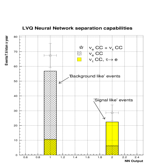
Combining MLP with LVQ
We have seen that LVQ networks returns a discrete output. The whole event sample is classified by the LVQ in two classes: signal-like and background-like. We can use the classification of a LVQ as a pre-classification for the MLP. A priori, it seems reasonable to expect an increase on the oscillation search sensitivity if we combine the LVQ and MLP approaches. The aim is to evaluate how much additional background rejection, from the contamination inside the signal-like sample, can be obtained by means of a MLP.
We present in Fig. 6.18 the MLP output for events classified as signal-like by the LVQ network (see Fig. 6.17). Applying a cut on the MLP output such that we get signal events (our usual reference point of 25% selection efficiency), we get background events, similar to what was obtained with the MLP approach alone. This outcome conclusively shows that, contrary to our a priori expectations, an event pre-classification, by means of a learning vector quantization neural network, does not help improving the discrimination capabilities of a multi-layer perceptron.
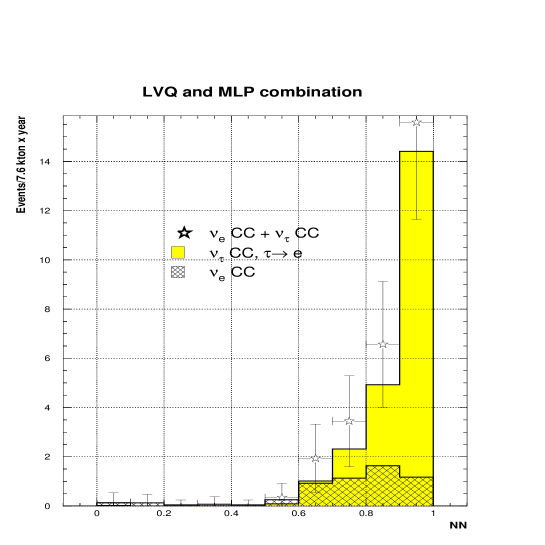
6.3 appearance discovery potential
We have studied several pattern recognition techniques applied to the particular problem of searching for oscillations. Based on discovery criteria, similar to the ones proposed in [135] for statistical studies of prospective nature, we try to quantify how much the discovery potential varies depending on the statistical method used.
We define and as the average number of expected signal and background events, respectively. With this notation, the discovery criteria are defined as:
-
1.
We require that the probability for a background fluctuation, giving a number of events equal or larger than , be smaller than (where is , the usual criteria applied for Gaussian distributions).
-
2.
We also set at which confidence level , the distribution of the total number of events with mean value fulfills the background fluctuation criteria stated above.
For instance, if is and is , we are imposing that of the times we repeat this experiment, we will observe a number of events which is or more above the background expectation.
For all the statistical techniques used, we fix = and =. In this way we can compute the minimum number of events needed to establish that, in our particular example, a direct oscillation has been discovered at the CNGS beam.
In Tab. 6.7 we compare the number of signal and background events obtained for the multi-layer perceptron and the multi-dimensional likelihood approaches after 5 years of data taking with a 3 kton detector. We also compare the minimum exposure needed in order to claim a discovery. The minimum exposure is expressed in terms of a scale factor , where means a total exposure of ktonyear. For the multi-layer perceptron approach (), a statistically significant signal can be obtained after a bit more than four years of data taking. On the other hand, the multi-dimensional likelihood approach requires 5 full years of data taking to claim a discovery. Therefore, when applied to the physics quest for neutrino oscillations, neural network techniques are more performing than classic statistical methods.
| Multi-layer | Multi-dimensional | |
| Perceptron | Likelihood | |
| # Signal | 12.9 | 12.9 |
| # Background | 0.66 | 1.1 |
| factor | 0.86 | 1.01 |
Conclusions
We have considered the general problem of oscillation search based on kinematic criteria to assess the performance of several statistical pattern recognition methods.
Two are the main conclusions of this study:
-
•
An optimal discrimination power is obtained using only the following variables: , and and their correlations. Increasing the number of variables (or combinations of variables) only increases the complexity of the problem, but does not result in a sensible change of the expected sensitivity.
-
•
Among the set of statistical methods considered, the multi-layer perceptron offers the best performance.
As an example, we have considered the case of the CNGS beam and appearance search (for the decay channel) using a very massive (3 kton) Liquid Argon TPC detector. Fig. 6.19 compares the discrimination capabilities of multi-dimensional likelihood and multi-layer perceptron approaches. We see that, for the low background region, the multi-layer perceptron gives the best sensitivity. For instance, choosing a selection efficiency of 25% as a reference value, we expect a total of CC () signal and CC background. Compared to multi-dimensional likelihood predictions, this means a 60% reduction on the number of expected background events. Hence, using a multi-layer perceptron, four years of data taking will suffice to get a statistically significant signal, while five years are needed when the search approach is based on a multi-dimensional likelihood.
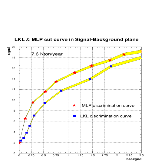
Conclusions
The results of this dissertation involve different aspects of Neutrino Physics. After a brief review of the main theoretical topics on neutrino interactions and the problem of their masses, a phenomenological study of the possibilities offered by future lepton colliders for the exploration of the limits on the mixing of light and new heavy neutrinos is presented. Afterwards we have focused our interest on experimental Neutrino Physics with LAr detectors, which is the main issue of this thesis. A sound and innovative work has been carried out in the development of the LAr technique and the necessary tools to perform Physics analyses, thus establishing the high potentiality of these detectors for the study of Neutrino Physics.
Assuming the possibility of the existence of heavy neutrinos with masses of few hundreds of GeV, we have analysed the contribution of these neutrinos to electroweak process in future lepton colliders, exploring the limits on heavy neutrino mixing and masses. We have studied the ILC potential for their detection in the process , taking into account the SM background and the effects of ISR and breamstrahlung, paying special attention to the relevance of the final state lepton flavour and initial beam polarization. Using a parton simulation it has been shown that it is possible to observe a heavy neutrino signal in this final state if it has a mixing with the electron , and a mass below GeV. Although a mixing with the electron of this size is necessary to observe a heavy neutrino at ILC, the signal may be more visible in the muon or tau channel if it also has a relatively large coupling to them. The production cross sections and then the discovery limits do not depend on the Dirac or Majorana nature of the heavy neutrino. These non-decoupled heavy neutrinos do not explain the observed light neutrino masses nor the baryon asymmetry of the universe. In this sense this search for heavy neutrinos at large lepton colliders is complementary to the joint experimental effort for determining the light neutrino properties, and in particular the neutrino mixing matrix (Ref [1]).
Thereafter, in the bulk of the dissertation, we have been mainly concentrated on the study of the Physics potential of LAr TPCs. We have developed a set of tools and procedures which makes possible the calorimetric and 3D reconstruction of ionizing events occurring within the chamber. These tools have shown an excellent performance working on events of low-multiplicity composed of several well defined tracks.
The technical operation of a 50 liter LAr TPC prototype, exposed to a multi-GeV neutrino beam, was rather good: The LAr purity was kept stable at a high-level during the whole data taking period and the electronic read-out configuration supplied an unbeatable signal-background ratio with no saturation of the electronic response, allowing an excellent imaging of the ionizing events.
The 50L TPC offered the opportunity to measure and reconstruct for first time beam neutrino interactions using the LAr technique. Due to the smallness of the prototype, a joint operation with the NOMAD detector acting as a muon spectrometer downstream of the TPC has been necessary in order to measure the high energy muons resulting from the neutrino interactions. Before the data analyses, a careful calibration of the TPC was done. All the needed parameters (the electron drift velocity, the alignment angles with respect to the beam, the electron lifetime and the recombination factors) were successfully obtained.
During its operation, the 50L TPC gathered a substantial sample of neutrino interactions in the multi-GeV region, with a sizable amount of low-multiplicity events. From the whole sample of CC events, we have selected a set of events called the golden sample. They are events having a clear two prong topology with a muon leaving the chamber and an identified contained proton. This sample contains 86 successfully reconstructed events and, in spite of its limited size, they have made possible to study the accuracy of our current Monte-Carlo models for the interactions of neutrinos with nuclear matter. We expect that most of these events come from quasi-elastic neutrino interactions, but there is also a sizable background coming from deep-inelastic and resonant events. Thanks to the superb reconstruction capabilities of the LAr TPC, the kinematical distributions of the events have been obtained with high resolution. This allows to discriminate between models with a full description of nuclear effects and naive approaches that only include Fermi motion and Pauli blocking (Ref. [2]).
On the other hand, the collected sample of golden events gives us the opportunity of measuring for first time the quasi-elastic CC cross section using a LAr TPC. To this purpose a precise knowledge of the beam composition, the beam profile, the exposition time, trigger efficiencies, acceptance cuts, event selection rates and background ratios was needed. In addition, a careful evaluation of the systematic errors entering in the computation has been done exploiting a full Monte-Carlo simulation of the neutrino beam, the nuclear effects and the experimental set-up. Our measurement of the total QE charged-current cross section (Ref. [3]) is
This value agrees with previous measurements of this reaction reported in the literature, and it stands as the first Physics measurement ever done with a LAr TPC using a neutrino beam from an accelerator.
Finally, given the excellent reconstruction capabilities of the LAr TPC technique and the accuracy in the reconstruction of the kinematic variables in the plane transverse to the incoming neutrino, we have evaluated our capability to perform a oscillation search based on kinematical criteria. A systematic assessment of the performance of several statistical pattern recognition methods shows that an optimal discrimination power is obtained using only three variables and their correlations: The visible energy (), the transverse missed momentum () and the fraction of transverse momentum carried by the prong lepton (). Moreover, among the set of statistical methods considered, the multi-layer perceptron offers the best performance. Considering the case of the appearance search at the CNGS neutrino beam using a very massive (3 kton) Liquid Argon TPC detector, we expect a total of CC () signal and CC background after 5 years running. This means a 60% reduction of the number of expected background events with respect to other broadly use methods in Particle Physics like for example, multi-dimensional likelihoods (Ref. [4]).
Appendix A Electroweak interactions
The standard electroweak model is based on the gauge symmetry group , and the corresponding gauge bosons , and . After spontaneus symmetry breaking and the usual redefinition of the gauge fields [9], the Lagrangian which describes the electroweak gauge interactions for fermions reads:
| (A.1) |
where is the usual doublet of the fermion family, being and the raising and lowering operators of the same representation. The first line of Eq. (A.1) describes charge current (CC) interactions, while the second one rules the neutral currents (NC); the electromagnetic interactions are governed by the third term.
A.1 Charged Current Interactions
In the SM left-handed fermions are put together in three different families of doublets, while the right-handed components are singlets. Thus, the emission of a charged vector boson causes a transition between the left-handed fermions within the weak isospin doublet .
These processes and are governed by the Lagrangian
| (A.2) |
with the vector field operators111 is the operator that annihilates a or creates a . and the fermion current summed over the 3 lepton and quark doublets:
| (A.3) |
Here, the field operators have been replaced by the particle symbols (, ) for simplicity. The projection operator assures that only leptons with left-handed chirality take part in the process
| (A.4) |
For massive fermions the weak isospin eigenstates are generally a mixture of the mass eigenstates. The basic mechanism by means of which fermions adquire mass in the SM preserving the gauge symmetry is through Yukawa couplings with the Higgs boson [8]. It is always possible to choose a fermion basis where just the fermions of one of the isospin eigenstates are rotated respect to their mass eigenstates after symmetry breaking. Thus, without loss of generality, only one unitary -matrix operating in the is needed in order to describe the relation between interaction and mass eigenstates:
| (A.5) |
It could have been equivalently done with the fermions. Therefore, quarks and lepton basis are usually choosen so that charge leptons (e ) and up quarks ( ) coincide with their mass eigenstates, while their opposite weak isospin partners are rotated respect to their mass eigenstates. The charged fermion current can now be rewritten as a sum over the observed fermions
| (A.6) |
The quarks and charged leptons correspond to the mass eigenstates shown in Tab. 1.1. Eq. (A.6) essentially implies that charged current weak interactions cause transitions between quarks or leptons of the three generations.
A.1.1 Charged Leptonic Current
The recently found neutrino oscillations imply that the neutrinos , and are not the mass eigenstates . This means that the mixing matrix is not diagonal [9]. In fact, current limits indicate mixing angles which correspond to almost maximal mixing for and . Also, there might be more than three neutrinos taking part in the mixing (see Sec 1.2). Because of the small neutrino masses and since they interact only weakly, the mass eigenstates are not yet directly observable, but have to be determined by means of oscillation rates and cosmological measurements. The experimental evidence in favor of oscillations of solar (KamLAND) and atmospheric (K2K) neutrinos can be accommodated in the SM with three massive neutrinos. The charged leptonic current is often also written in terms of the weak eigenstates:
| (A.7) |
A.1.2 Charged Quark Current
The mixing in the quark sector is described by the Cabibbo-Kobayashi-Maskawa (CKM) matrix:
| (A.8) |
The squared matrix elements give the probability of the quark to change into the quark . Conservation of probability requires the CKM matrix to be unitary. In principle, the individual matrix elements can all be measured in weak decays of the relevant quarks or in deep inelastic neutrino-nucleon scattering. The 90 % confidence limits on the magnitude of the matrix elements, as given in [9], are
| (A.9) |
In contrast with the leptonic sector, the mixing in the quark sector is easily observable, since the mass differences are bigger and the quarks interact also via the strong force.
A.2 Neutral Current Interactions
The boson, just as the photon, is a mixture of the neutral gauge field of the symmetry group (the other two weak bosons being and ) and the gauge field of the symmetry group. The form of the weak neutral current, therefore, also depends on whether or not the fermions carry charge. The corresponding Lagrangian is given by
| (A.10) |
where is the Weinberg angle defined by . The neutral current is summed over all fermions
| (A.11) |
and
| (A.12) |
where is the weak isospin of the left-handed fermion, i. e. , and is the charge of the fermion in units of .
Appendix B Calculation of the process with heavy neutrinos
Following the notation that we introduced in Sec. 1.4 for the neutrino mixing matrix (Eq. (1.32)), we write down the extended (MNS) matrix [26, 136] as . This matrix parameterises the charged and neutral current gauge interactions. On the other hand, the neutrino mass eigenstates have been renamed as in that Section in order to make explicit the distintion between the light () and the heavy () sectors. The electroweak Lagrangian is then written as
| (B.3) | |||||
| (B.6) |
In the evaluation of , with , we will only consider the contributions from the diagrams in Fig. B.1, neglecting diagrams with four fermions in the final state but with not resulting from a decay. At any rate, we have checked that the corresponding contributions are negligible in the phase space region of interest. The discovery of a new heavy neutrino in requires its observation as a peak in the invariant mass distribution, otherwise the irreducible SM background is overwhelming. This requires to reconstruct the , what justifies to consider production (instead of general four fermion production), with decaying hadronically.
Let us discuss the contributions and sizes of the different diagrams for in Fig. B.1 and what we can learn from this type of processes at ILC. The first four diagrams are SM contributions. Diagrams 5, are present within the SM, mediated by a light neutrino, but they can also involve a heavy one. Diagrams 6 and 10 are exclusive to Majorana neutrino exchange. The SM contribution has a substantial part from resonant production, diagrams 4 and 8, especially for final states with . The heavy neutrino signal is dominated by diagrams 5 and 6 with produced on its mass shell, because the enhancement of the amplitude partially cancels the mixing angle factor in the decay vertex, yielding the corresponding branching ratio. It must be remarked that the -channel production diagram 7 is negligible (few per mille) when compared to the -, -channel diagrams 5 and 6. This behaviour is general, because the -channel propagator is fixed by the large collider energy and suppresses the contribution of this diagram, whereas the - and -channel propagators do not have such suppression. Since both diagrams 5 and 6 involve an vertex to produce a heavy neutrino, only in the presence of this interaction the signal is observable. Once the heavy neutrino is produced, it can decay to with , being the corresponding branching ratios in the ratio .

In case that the signal is dominated by and channel on-shell production (the only situation in which it is observable), negative electron polarisation and positive positron polarisation increase its statistical significance. For the signal contributions alone we have (for GeV, ), with . For the SM process, , . In the limit of perfect beam polarisations , , the signal is enhanced with respect to the background by a factor of 1.05 and, what is more important, the ratio increases by a factor of two. Using right-handed electrons and left-handed positrons decreases the ratio by a factor of 8, and by a factor of 50. On the other hand, if the neutrino does not mix with the electron but mixes with the muon or tau, the behaviour is the opposite. Since the only contribution comes from diagram 7 the use of left-handed positrons and right-handed electrons actually increases the signal, while reducing the SM cross section for this process [137]. This case is of limited practical interest, since for the signal is barely observable.
We finally point out that the signal cross section exhibits little dependence on the heavy neutrino mass, except close to the kinematical limit [138, 139], and the final results are almost independent of within the range 200-400 GeV [43]. For our calculations we take GeV. In contrast with what has been claimed in the literature [140], we find equal production cross sections for Dirac and Majorana neutrinos to a very good approximation. The reason is easy to understand: while in the present case the signal is strongly dominated by diagrams 5 and 6 (which give equal contributions to the cross section and do not interfere because light neutrino masses can be safely neglected), for a Dirac neutrino only diagram 5 is present. On the other hand, the width of a Dirac neutrino is one half of the width of a Majorana neutrino with the same mixing angles [43].
Generation of signals
The matrix elements for are calculated using HELAS [141], including all spin correlations and finite width effects. We sum SM and heavy neutrino-mediated diagrams at the amplitude level. The charge conjugate process is included in all our results unless otherwise noted. We assume a CM energy of 500 GeV, with electron polarisation and positron polarisation . The luminosity is taken as 345 fb-1 per year [142]. In our calculations we take into account the effects of ISR [143] and beamstrahlung [144, 145]. For the design luminosity at 500 GeV we use the parameters , [142]. The actual expressions for ISR and beamstrahlung used in our calculation are collected in Ref. [146]. We also include a beam energy spread of 1%.
In final states with leptons, we select decays to , and mesons (with a combined branching fraction of 55% [9]), in which a single is produced, discarding other hadronic and leptonic decays. We simulate the decay assuming that the meson and momenta are collinear (what is a good approximation for high energies) and assigning a random fraction of the momentum to the meson, according to the probability distributions [147]
| (B.7) |
for pions, and
| (B.8) |
for and mesons, where . We assume a jet tagging efficiency of 50%.
We simulate the calorimeter and tracking resolution of the detector by performing a Gaussian smearing of the energies of electrons, muons and jets, using the specifications in Ref. [148],
| (B.9) |
respectively, where the two terms are added in quadrature and the energies are in GeV. We apply kinematical cuts on transverse momenta, GeV, and pseudorapidities , the latter corresponding to polar angles . To ensure high momenta (so that the meson resulting from its decay is effectively collinear) we require GeV for jets. We reject events in which the leptons or jets are not isolated, requiring a “lego-plot” separation . For the Monte Carlo integration in 6-body phase space we use RAMBO [149].
In final states with electrons and muons the light neutrino momentum is determined from the missing transverse and longitudinal momentum of the event and the requirement that (despite ISR and beamstrahlung, the missing longitudinal momentum approximates with a reasonable accuracy the original neutrino momentum). In final states with leptons, the reconstruction is more involved, due to the additional neutrino from the decay. We determine the “first” neutrino momentum and the fraction of the momentum retained by the jet using the kinematical constraints
| (B.10) |
in obvious notation. These constraints only hold if ISR and beamstrahlung are ignored, and in the limit of perfect detector resolution. When solving them for the generated Monte Carlo events we sometimes obtain or . In the first case we arbitrarily set , and in the second case we set , which is the average momentum fraction of the jets. With the procedure outlined here, the reconstructed momentum reproduces with a fair accuracy the original one, while the obtained is often quite different from its original value.
References
- [1] F. del Aguila and J. A. Aguilar-Saavedra and A. Martínez de la Ossa and D. Meloni, Flavour and polarisation in heavy neutrino production at e+ e- colliders, Phys. Lett. B613 (2005) 170–180, [hep-ph/0502189].
- [2] ICARUS-MILANO Collaboration, Performance of a liquid argon time projection chamber exposed to the CERN West Area Neutrino Facility neutrino beam, Phys. Rev. D74 (2006) 112001, [physics/0609205].
- [3] ICARUS-MILANO Collaboration, Measurement Of The Quasi-Elastic Muon Neutrino Charged Current Cross Section With A Liquid Argon TPC In The CERN WANF Neutrino Beam, . ICARUS-TM/06-04. [Submitted for publication].
- [4] A. Bueno and A. Martínez de la Ossa and S. Navas-Concha and A. Rubbia, Statistical pattern recognition: Application to oscillation searches based on kinematic criteria, JHEP 11 (2004) 014, [hep-ph/0407013].
- [5] M. E. Peskin and D. V. Schroeder, An Introduction to Quantum Field Theory. Advanced-Wesley Publishing Company, 1995.
- [6] F. Halzen and A. D. Martin, Quarks and Leptons: An Introductory Course in Modern Particle Physics. John Wiley and sons, 1984.
- [7] D. Griffiths, Introduction to Elementary Particles. John Wiley and sons, 1987.
- [8] W. N. Cottingham and D. A. Greenwood, An introduction to the Standard Model of Particle Physics. Cambridge University Press, 1998.
- [9] Particle Data Group Collaboration, W. M. Yao and others, Review of particle physics, J. Phys. G33 (2006) 1–1232.
- [10] D. H. Perkins, Introduction to High Energy Physics. Cambridge University Press, 4th ed., 1999.
- [11] P. Langacker (Ed.), Precision Tests of the Standard Electroweak Model, vol. 14 of Advanced Series on Directions in High Energy Physics. World Scientific, 1995.
- [12] Super-Kamiokande Collaboration, Y. Fukuda and others, Evidence for oscillation of atmospheric neutrinos, Phys. Rev. Lett. 81 (1998) 1562–1567, [hep-ex/9807003].
- [13] MACRO Collaboration, G. Giacomelli and M. Giorgini, Atmospheric neutrino oscillations in MACRO, hep-ex/0110021.
- [14] Soudan-2 Collaboration, W. A. Mann, New results on atmospheric neutrinos from Soudan 2, Nucl. Phys. Proc. Suppl. 91 (2001) 134–140, [hep-ex/0007031].
- [15] SNO Collaboration, Q. R. Ahmad and others, Measurement of the charged current interactions produced by B-8 solar neutrinos at the Sudbury Neutrino Observatory, Phys. Rev. Lett. 87 (2001) 071301, [nucl-ex/0106015].
- [16] SNO Collaboration, Q. R. Ahmad and others, Direct evidence for neutrino flavor transformation from neutral-current interactions in the Sudbury Neutrino Observatory, Phys. Rev. Lett. 89 (2002) 011301, [nucl-ex/0204008].
- [17] SNO Collaboration, Q. R. Ahmad and others, Measurement of day and night neutrino energy spectra at SNO and constraints on neutrino mixing parameters, Phys. Rev. Lett. 89 (2002) 011302, [nucl-ex/0204009].
- [18] R. N. Mohapatra and P. B. Pal, Massive Neutrinos In Physics And Astrophisics. World Scientific Lecture Notes in Physics - Vol. 72, 3th ed., 2004.
- [19] G. C. Branco and L. Lavoura and J. P. Silva, CP Violation. Oxford university Press, ed., 1999.
- [20] C. Giunti and M. Laveder, Neutrino mixing, hep-ph/0310238.
- [21] G. Gelmini and E. Roulet, Neutrino Masses, Rept. Prog. Phys. 58 (1995) 1207–1266, [hep-ph/9412278].
- [22] E. Majorana, Theory Of The Symmetry Of Electrons And Positrons, Nuovo Cim. 14 (1937) 171–184.
- [23] M. Gell-Mann, P. Ramond and R. Slansky, Supergravity. North Holland, Amsterdam, 1979.
- [24] B. Pontecorvo, Inverse beta processes and nonconservation of lepton charge, Sov. Phys. JETP 7 (1958) 172–173.
- [25] G. Danby and J. M. Gaillard and K. Goulianos and L. M. Lederman and N. Mistry and M. Schwartz and J. Steinberger, Observation of High-Energy Neutrino Reactions and the Existence of Two Kinds of Neutrinos, Phys. Rev. Lett. 9 (1962), no. 1 36–44.
- [26] Z. Maki and M. Nakagawa and S. Sakata, Remarks on the unified model of elementary particles, Prog. Theor. Phys. 28 (1962) 870.
- [27] M. Fukugita and T. Yanagida, Baryogenesis without Grand Unification, Phys. Lett. B174 (1986) 45.
- [28] G. C. Branco, R. Gonzalez Felipe, F. R. Joaquim, and M. N. Rebelo, Leptogenesis, CP violation and neutrino data: What can we learn?, Nucl. Phys. B640 (2002) 202–232, [hep-ph/0202030].
- [29] A. Pilaftsis and T. E. J. Underwood, Resonant leptogenesis, Nucl. Phys. B692 (2004) 303–345, [hep-ph/0309342].
- [30] R. Gonzalez Felipe, F. R. Joaquim, and B. M. Nobre, Radiatively induced leptogenesis in a minimal seesaw model, Phys. Rev. D70 (2004) 085009, [hep-ph/0311029].
- [31] T. Hambye, J. March-Russell, and S. M. West, TeV scale resonant leptogenesis from supersymmetry breaking, JHEP 07 (2004) 070, [hep-ph/0403183].
- [32] L. Boubekeur, T. Hambye, and G. Senjanovic, Low-scale leptogenesis and soft supersymmetry breaking, Phys. Rev. Lett. 93 (2004) 111601, [hep-ph/0404038].
- [33] A. Abada, H. Aissaoui, and M. Losada, A model for leptogenesis at the TeV scale, Nucl. Phys. B728 (2005) 55–66, [hep-ph/0409343].
- [34] W. Buchmuller, P. Di Bari, and M. Plumacher, Leptogenesis for pedestrians, Ann. Phys. 315 (2005) 305–351, [hep-ph/0401240].
- [35] C. Giunti, Status of neutrino masses and mixing, Eur. Phys. J. C33 (2004) s852–s856, [hep-ph/0309024].
- [36] M. C. Gonzalez-Garcia and C. Pena-Garay, Three-neutrino mixing after the first results from K2K and KamLAND, Phys. Rev. D68 (2003) 093003, [hep-ph/0306001].
- [37] N. Cabibbo, Time Reversal Violation in Neutrino Oscillation, Phys. Lett. B72 (1978) 333.
- [38] S. P. Mikheev and A. Yu. Smirnov, Resonance enhancement of oscillations in matter and solar neutrino spectroscopy, Sov. J. Nucl. Phys. 42 (1985) 913–917.
- [39] L. Wolfenstein, Neutrino oscillations in matter, Phys. Rev. D17 (1978) 2369.
- [40] S. Bergmann and A. Kagan, Z-induced FCNCs and their effects on neutrino oscillations, Nucl. Phys. B538 (1999) 368–386, [hep-ph/9803305].
- [41] B. Bekman and J. Gluza and J. Holeczek and J. Syska and M. Zralek, Matter effects and CP violating neutrino oscillations with non-decoupling heavy neutrinos, Phys. Rev. D66 (2002) 093004, [hep-ph/0207015].
- [42] F. del Aguila and J. A. Aguilar-Saavedra and R. Pittau, Neutrino physics at large colliders, J. Phys. Conf. Ser. 53 (2006) 506–527, [hep-ph/0606198].
- [43] F. del Aguila and J. A. Aguilar-Saavedra, production at CLIC: A window to TeV scale non- decoupled neutrinos, JHEP 05 (2005) 026, [hep-ph/0503026].
- [44] P. Langacker and D. London, Lepton-number violation and massless nonorthogonal neutrinos, Phys. Rev. D38 (Aug, 1988) 907–916.
- [45] J. G. Korner and A. Pilaftsis and K. Schilcher, Leptonic flavor changing Z0 decays in SU(2) x U(1) theories with right-handed neutrinos, Phys. Lett. B300 (1993) 381–386, [hep-ph/9301290].
- [46] E. Nardi and E. Roulet and D. Tommasini, Limits on neutrino mixing with new heavy particles, Phys. Lett. B327 (1994) 319–326, [hep-ph/9402224].
- [47] A. Ilakovac and A. Pilaftsis, Flavor violating charged lepton decays in seesaw-type models, Nucl. Phys. B437 (1995) 491, [hep-ph/9403398].
- [48] D. Tommasini and G. Barenboim and J. Bernabeu and C. Jarlskog, Nondecoupling of heavy neutrinos and lepton flavor violation, Nucl. Phys. B444 (1995) 451–467, [hep-ph/9503228].
- [49] J. I. Illana and T. Riemann, Charged lepton flavor violation from massive neutrinos in decays, Phys. Rev. D63 (Feb, 2001) 053004.
- [50] G. C. Branco and D. Delepine and B. Nobre and J. Santiago, Extra dimensions, isosinglet charged leptons and neutrino factories, Nucl. Phys. B657 (2003) 355–377, [hep-ph/0209263].
- [51] R. N. Mohapatra, Particle physics implications of neutrinoless double beta decay, Nucl. Phys. Proc. Suppl. 77 (1999) 376–385, [hep-ph/9808284].
- [52] D. A. Glaser, Some Effects of Ionizing Radiation on the Formation of Bubbles in Liquids, Phys. Rev. 87 (1952) 665.
- [53] D. A. Glaser, Bubble Chamber Tracks of Penetrating Cosmic-Ray Particles, Phys. Rev. 91 (1953) 762–763.
- [54] D. A. Glaser Nuovo Cim. Suppl. 2 (1954) 361.
- [55] C. Rubbia, “The Liquid-Argon Time Projection Chamber: A New Concept For Neutrino Detector.” 1977.
- [56] ICARUS Collaboration, “ICARUS-I. A proposal for the Gran Sasso laboratory.” Proposal, INFN/AE-85/7, Frascati (Italy, 1985).
- [57] ICARUS Collaboration, “ICARUS-II. A second generation proton decay experiment and neutrino observatory at the Gran Sasso laboratory.” Proposal, VOL I (1993) II (1994), LNGS-94/99.
- [58] O. Bunemann and J. A. Harvey Can. J. Res. 27 (1949) 191.
- [59] E. Gatti and Others IEEE Trans. Nucl. Sci. 26 (1970) 2910.
- [60] A. Bueno and S. Navas-Concha, “Particle identification in ICARUS.” ICARUS-TM/04-09, 2004.
- [61] P. Cennini and others, Detection of scintillation light in coincidence with ionizing tracks in a liquid argon time projection chamber, Nucl. Instr. Meth. A432 (1999) 240–248.
- [62] P. Bennetti and others, The ICARUS RD program and results, Nucl. Instr. Meth. A327 (1993) 173–177.
- [63] P. Bennetti and others, A 3 ton liquid argon time projection chamber, Nucl. Instr. Meth. A332 (1993) 395.
- [64] ICARUS Collaboration, P. Cennini and others, Performance of a 3-ton liquid argon time projection chamber, Nucl. Instr. Meth. A345 (1994) 230–243.
- [65] ICARUS Collaboration, P. Cennini and others, A 3-D image chamber for the liquid argon TPC based on multi-layer printed circuit board, Nucl. Instr. Meth. A346 (1994) 550–556.
- [66] E. Buckley and others, A study of ionization electrons drifting over large distances in liquid argon, Nucl. Instr. Meth. Phys. Res. A (, 1989) 364–372. .
- [67] A. Bettini and others, A Study of the factors affecting the electron lifetime in ultrapure liquid argon, Nucl. Instr. Meth. A305 (1991) 177–186.
- [68] ICARUS Collaboration, S. Amerio and others, Design, construction and tests of the ICARUS T600 detector, Nucl. Instr. Meth. A527 (2004) 329–410.
- [69] ICARUS Collaboration, The ICARUS experiment: A second-generation proton decay experiment and neutrino observatory at the Gran Sasso laboratory. Cloning of T600 modules to reach the design sensitive mass. (Addendum), LNGS-EXP 13/89 add. 2/01 (2001). CERN-SPSC-2002-027.
- [70] S. Ragazzi, “Request for a test of a liquid argon TPC on the neutrino beam.” CERN-SPSLC-96-57, 1996.
- [71] ICARUS Collaboration, P. Cennini and others, Argon purification in the liquid phase, Nucl. Instr. Meth. A333 (1993) 567–570.
- [72] G. Carugno and B. Dainese and F. Pietropaolo and F. Ptohos, Electron lifetime detector for liquid argon, Nucl. Instr. Meth. A292 (1990) 580–584.
- [73] P. Cennini and others, Improving the performance of the liquid argon TPC by doping with tetramethyl germanium, Nucl. Instr. Meth. A355 (1995) 660–662.
- [74] J. Rico, First Study of the Stopping Muon Sample with the ICARUS T600 Detector. PhD thesis, ETH, 2002. Ph.D. Dissertation.
- [75] W. H. Press and S. A. Teukolsky and W. T. Vettering and B. P. Flannery, Numerical Recipes in C++. The Art of Scientific Computing, .
- [76] F. James and M. Roos, ’MINUIT’ A System For Function Minimization And Analysis Of The Parameter Errors And Correlations, Comput. Phys. Commun. 10 (1975) 343–367.
- [77] D. G. Cassel and H. Kowalski, Pattern Recognition in Layered Track Chambers using a Tree Algorithm, Nucl. Instr. Meth. 185 (1981) 235.
- [78] C. Peterson, Track finding with Neural Networks, Nucl. Instr. Meth. A279 (1989) 537–545.
- [79] C. Peterson and T. Rognvaldsson, An Introduction to Artificial Neural Networks, 1991 CERN Scool Of Computing (1992) 113–170.
- [80] G. Stimpfl-Abele and L. Garrido, Fast Track finding with Neural Networks, Comput. Phys. Comm. 64 (1991) 46.
- [81] C. M. Bishop, Neural Networks for Pattern Recognition. Oxford university Press, 1995.
- [82] J. J. Hopfield and D. W. Tank, Neural computation of decisions in optimization problems, Biological Cybernetics 52 (1985) 141–152.
- [83] C. Peterson and J.R. Anderson, A mean field theory learning algorithm for neural networks, Complex Systems 1 (1987) 995–1019.
- [84] W. R. Leo, Techniques for Nuclear and Particle Physics Experiments. Springer-Verlag, 1987.
- [85] C. Grupen, Particle Detectors. Cambridge University Press, 1996.
- [86] W. Lohmann and R. Kopp and R. Voss, Energy Loss of muons in the energy range 1-GeV to 10000-GeV, . CERN-85-03.
- [87] D. H. Wilkinson, Ionization energy loss by charged particles. I: The Landau distribution, Nucl. Instr. Meth. A383 (1996) 513–515.
- [88] J. Birks, Theory and Practice of Scintillation Counting. Pergamon Press, New York, 1964.
- [89] ICARUS Collaboration, S. Amoruso and others, Study of electron recombination in liquid argon with the ICARUS TPC, Nucl. Instr. Meth. A523 (2004) 275–286.
- [90] S. Ragazzi, Request for a test of a liquid argon TPC on the neutrino beam, . CERN-SPSLC-96-57.
- [91] G. Acquistapace and others, The West area neutrino facility for CHORUS and NOMAD experiments: 1994 - 1997 operation, . CERN-ECP-95-014.
- [92] NOMAD Collaboration, J. Altegoer and others, The NOMAD experiment at the CERN SPS, Nucl. Instr. Meth. A404 (1998) 96–128.
- [93] CHORUS Collaboration, E. Eskut and others, The CHORUS experiment to search for oscillation, Nucl. Instr. Meth. A401 (1997) 7–44.
- [94] ICARUS Collaboration, A. Rubbia and others, A search programme of explicit nu oscillations with the ICARUS detector at long distances, . CERN-SPSLC-96-58.
- [95] ICARUS Collaboration, F. Arneodo and others, The ICARUS 50-l LAr TPC in the CERN nu beam, hep-ex/9812006.
- [96] A. Curioni, “Esposizione di una camera a proiezione temporale di 50 litri al fascio di neutrini del CERN.” Diploma Thesis, Milano, 1997.
- [97] B. Boschetti, “Studio sperimentale di interazioni di neutrino quasi-elastiche in argon liquido.” Diploma Thesis, Milano, 1997.
- [98] ICARUS-Milano Collaboration, A. Curioni, Experimental study of quasi-elastic neutrino interactions on Ar with a liquid Ar TPC exposed to the WANF neutrino beam, hep-ex/0603009.
- [99] NOMAD Collaboration, P. Astier and others, Prediction of neutrino fluxes in the NOMAD experiment, Nucl. Instr. Meth. A515 (2003) 800–828, [hep-ex/0306022].
- [100] L. Casagrande and others, The alignment of the CERN West Area neutrino facility, . CERN-96-06.
- [101] NOMAD Collaboration, J. Altegoer and others, The trigger system of the NOMAD experiment, Nucl. Instr. Meth. A428 (1999) 299–316.
- [102] M. Anfreville and others, The drift chambers of the Nomad experiment, Nucl. Instr. Meth. A481 (2002) 339–364, [hep-ex/0104012].
- [103] S. Navas-Concha and others, “A measurement of the electron Lifetime and the electron Recombination factor with the T600 data.” ICARUS-TM/02-04, 2002.
- [104] A. Rubbia, “NUX Code.” Talk at NuInt01, http://neutrino.kek.jp/nuint01, 2001.
- [105] A. Ferrari and A. Fasso and J. Ranft and P. R. Sala, FLUKA: A multi-particle transport code, . CERN-2005-010, INFN/TC-05/11, SLAC-R-773.
- [106] G. Battistoni and A. Ferrari and P. R. Sala, The Treatment of Nuclear Effects for Neutrino Interactions in the FLUKA Code, Acta Phys. Polonica B37 (2006) 2361.
- [107] GEANT4 Collaboration, S. Agostinelli and others, GEANT4: A simulation toolkit, Nucl. Instr. Meth. A506 (2003) 250–303.
- [108] R. Brun and F. Rademakers, ROOT: An object oriented data analysis framework, Nucl. Instr. Meth. A389 (1997) 81–86.
- [109] F. Cavanna and others, Neutrino nucleus interactions in the few-GeV region, Proceedings of NuInt04 (2004). Assergi, Italy.
- [110] P. Lipari, C. Keppel, and M. Sakuda Nucl. Phys. B (Proc. Suppl.) 139 (2005).
- [111] G. Battistoni and A. Ferrari and A. Rubbia and P. R. Sala, The FLUKA nuclear cascade model applied to neutrino interactions, Proceedings of NuInt02 (2002). University of California, Irvine.
- [112] P. R. Sala, “Private communication.”.
- [113] S. J. Barish and others, Study of neutrino interactions in hydrogen and deuterium: Description of the experiment and study of the reaction , Phys. Rev. D16 (1977) 3103.
- [114] S. Bonetti and others, Study of quasielastic reactions of neutrino and anti-neutrino in Gargamelle, Nuovo Cim. A38 (1977) 260–270.
- [115] N. J. Baker and others, Quasielastic neutrino scattering: A measurement of the weak Nucleon axial vector form-factor, Phys. Rev. D23 (1981) 2499–2505.
- [116] T. Kitagaki and others, High-energy quasielastic scattering in deuterium, Phys. Rev. D28 (1983) 436–442.
- [117] S. Belikov and others, Quasielastic neutrino and antineutrino scattering total cross-sections, axial-vector form-factor, Zeit. fur Phys. A320 (1985) 625.
- [118] J. Brunner and others, Quasielastic nucleon and hyperon production by neutrinos and antineutrinos with energies below 30 GeV, Zeit. fur Phys. C45 (1990) 551.
- [119] D. Allasia and others, Investigation of exclusive channels in neutrino / anti-neutrino deuteron charged current interactions, Nucl. Phys. B343 (1990) 285–309.
- [120] Super-Kamiokande Collaboration, Y. Ashie and others, Evidence for an oscillatory signature in atmospheric neutrino oscillation, Phys. Rev. Lett. 93 (2004) 101801, [hep-ex/0404034].
- [121] G. Acquistapace and others, The CERN neutrino beam to Gran Sasso (NGS): Conceptual technical design, . CERN-98-02.
- [122] OPERA Collaboration, M. Guler and others, OPERA: An appearance experiment to search for oscillations in the CNGS beam. Experimental proposal, . CERN-SPSC-2000-028, SPSC/P318, LNGS P25/2000.
- [123] R. Baldy and others, The CERN neutrino beam to Gran Sasso (NGS). (Addendum), . CERN-SL-99-034-DI.
- [124] A. Ferrari and I. Gil-Botella and A. Rubbia, “Implementation of T600 geometry and wire plane readout in FLUKA and the Neutron Background Captured Rate.” ICARUS-TM/01-05, 2005.
- [125] NOMAD Collaboration, P. Astier and others, A more sensitive search for oscillations in NOMAD, Phys. Lett. B453 (1999) 169–186.
- [126] Y. Ge and P. R. Sala and A. Rubbia, “ Separation in ICARUS Liquid Argon Time Projection Chamber.” ICARUS-TM/03-04, 2004.
- [127] ICANOE Collaboration, F. Arneodo and others, ICANOE: Imaging and calorimetric neutrino oscillation experiment: A proposal for a CERN-GS long baseline and atmospheric neutrino oscillation experiment, . INFN-AE-99-17, CERN/SPSC 99-25, SPSC/P314.
- [128] G. Cowan, Statistical data analysis. Oxford university Press, 1998.
- [129] S. Haykin, Neural Networks: A comprehensive foundation. Prentice Hall, 1999.
- [130] C. Peterson and T. Rognvaldsson, An Introduction to artificial neural networks, . Lectures given at 1991 CERN School of Computing, Ystad, Sweden, Aug 23 - Sep 2, 1991.
- [131] L. Ametller and L. Garrido and G. Stimpfl-Abele and P. Talavera and P. Yepes, Discriminating signal from background using neural networks. Application to top-quark search at the Fermilab Tevatron, Phys. Rev. D54 (1996) 1233–1236, [hep-ph/9603269].
- [132] P. Chiappetta and P. Colangelo and P. De Felice and G. Nardulli and G. Pasquariello, Higgs search by neural networks at LHC, Phys. Lett. B322 (1994) 219–223, [hep-ph/9401343].
- [133] R. Brun and others, “PAW neural network interface. MLPfit package (version 1.33).” http://home.cern.ch/schwind/MLPfit.html.
- [134] B. Roe, Event selection using an extended Fisher discriminant method, ECONF C030908 (2003) WEJT003.
- [135] J. J. Hernandez and S. Navas-Concha and P. Rebecchi, Discovery limits in prospective studies, Nucl. Instr. Meth. A372 (1996) 293–296.
- [136] B. Pontecorvo, Mesonium and anti-mesonium, Sov. Phys. JETP 6 (1957) 429.
- [137] D. Meloni, Neutrinos as a probe of physics beyond the standard model, Acta Phys. Polon. B35 (2004) 2781–2793.
- [138] J. Gluza and M. Zralek, Heavy neutrinos production and decay in future e+ e- colliders, Phys. Rev. D55 (1997) 7030–7037, [hep-ph/9612227].
- [139] J. Gluza and M. Zralek, Neutrino production in e+ e- collisions in a left-right symmetric model, Phys. Rev. D48 (1993) 5093–5105.
- [140] F. M. L. Almeida and Y. A. Coutinho and J. A. Martins Simões and M. A. B. do Vale, Neutral heavy lepton production at next high energy linear colliders, Phys. Rev. D63 (Mar, 2001) 075005.
- [141] H. Murayama and I. Watanabe and K. Hagiwara, HELAS: HELicity amplitude subroutines for Feynman diagram evaluations, . KEK-91-11.
- [142] International Linear Collider Technical Review Committee 2003 Report, . http://www.slac.stanford.edu/xorg/ilc-trc/2002/2002/report/03rep.htm.
- [143] M. Skrzypek and S. Jadach, Exact and approximate solutions for the electron nonsinglet structure function in QED, Z. Phys. C49 (1991) 577–584.
- [144] M. Peskin. Linear Collider Collaboration Note LCC-0010.
- [145] K. Yokoya and P. Chen. SLAC-PUB-4935. Presented at IEEE Particle Accelerator Conference, Chicago, Illinois, Mar 20-23, 1989.
- [146] J. A. Aguilar-Saavedra and A. M. Teixeira, Testing the Majorana nature of neutralinos in supersymmetric theories, Nucl. Phys. B675 (2003) 70–98, [hep-ph/0307001].
- [147] J. D. Anderson and M. H. Austern and R. N. Cahn, Measurement of Z-prime couplings at future hadron colliders through decays to tau leptons, Phys. Rev. D46 (1992) 290–302.
- [148] G. Alexander and others, TESLA Technical Design Report Part 4, . DESY-01-011.
- [149] R. Kleiss and W. J. Stirling and S. D. Ellis, A new Monte Carlo treatment of multiparticle phase space at high energies, Comput. Phys. Commun. 40 (1986) 359–373.