Abstract

We present results of a search for for the anomalous production of events containing a high-transverse momentum charged lepton ($\ell$, either $e$ or $\mu$) and photon ($\gamma$), accompanied by missing transverse energy (${\rm\not\!E}_{\rm T}$), and/or additional leptons and photons, and jets (X). We use the same kinematic selection criteria as in a previous CDF search, but with a substantially larger data set, $305$ $pb^{-1}$, a $\rm p{\bar{p}}$ collision energy of 1.96 $\mathrm{Te\kern-1.00006ptV}$, and the upgraded CDF II detector. We find $42$ $\ell\gamma\mbox{${\rm\not\!E}_{\rm T}$}$ events versus a standard model expectation of $37.3\pm 5.4$ events. The level of excess observed in Run I, 16 events with an expectation of 7.6 $\pm$ 0.7 events (corresponding to a 2.7$\sigma$ effect), is not supported by the new data. In the signature of $\ell\ell\gamma+X$ we observe $31$ events versus an expectation of $23.0\pm 2.7$ events. In this sample we find no events with an extra photon or ${\rm\not\!E}_{\rm T}$ and so find no events like the one $ee\gamma\gamma\mbox{${\rm\not\!E}_{\rm T}$}$ event observed in Run I.

…to my dear grandmother…

Introduction

An important test of the standard model (SM) of particle physics [1] is to measure and understand the properties of the highest momentum-transfer particle collisions, which correspond to measurements at the shortest distances. The predicted high energy behavior of the SM, however, becomes unphysical at an interaction energy on the order of several TeV. These phenomena beyond the SM may involve new elementary particles, new fundamental forces, and/or a modification of space-time geometry. These new phenomena are likely to show up as an anomalous production rate of a combination of the known fundamental particles.

The unknown nature of possible new phenomena in the energy range accessible at the Tevatron is the motivation for a search strategy that does not focus on a single model of new physics, but presents a wide net for new phenomena. We compared SM predictions with the rates measured at the Tevatron with the CDF detector for final states with at least one high-PT lepton (e or $\mu$) and photon ($\gamma$), plus other detected objects (leptons, photons, jets, and missing transverse energy, ${\rm\not\!E}_{\rm T}$). A priori definition of selection cuts for the search allows to test Run I anomalies, such as the observation of an event consistent with the production of two energetic photons, two energetic electrons, and large ${\rm\not\!E}_{\rm T}$ (the “$ee\gamma\gamma\mbox{${\rm\not\!E}_{\rm T}$}$ event”), in Run II data. Another intriguing Run I result that is important to test is a 2.7$\sigma$ excess above the Standard Model expectations in the $\ell\gamma\mbox{${\rm\not\!E}_{\rm T}$}$ signature [2, 3].

The Fermilab Tevatron has the highest center-of-mass energy collisions (per nucleon) of any accelerator to date, and thus has the potential to discover new physics. The upgraded CDF II detector provides us better solid angle coverage and particle identification. The production of two vector gauge bosons, precisely predicted in the Standard Model, provides a set of signatures in which to search for the production of new particles which couple to the SM gauge sector (the top quark being the last new example).

This analysis has been done with 305 $pb^{-1}$ of $\rm p{\bar{p}}$ collisions at ${\sqrt{s}}$= 1.96 $\mathrm{Te\kern-1.00006ptV}$, collected with CDF detector at the Tevatron, Fermilab between March 23, 2002 and August 22, 2004. The main results of this thesis have been published in  [4, 5, 6]. Standard Model $W\gamma$ and $Z\gamma$ production CDF Run II results are published in [7]. The status of the Lepton+Photon+X search has been presented at the APS Conference (Philadelphia, 2003). The results have been presented at the SUSY 2005 conference (Durham, 2005) [8], the International School of Subnuclear Physics (Erice, 2005) [5], Lake Louise Winter Institute (2006) [9], and also at the CDF Collaboration Meeting (Sitges, 2005) and at the Exotics, Photon and Very Exotic Phenomena working group meetings.

At the International School of Subnuclear Physics (Erice, 2005) I havereceived the “New Talents” Award for an Original Work in Experimental Physics for the talk “Search for New Physics in Photon Final states”. The work has been reviewed and approved for publication in [4, 5] by G. t’Hooft, 1999 Nobel Laureate in Physics.

One of the most important tools for a better understanding of the events that could possibly be New Physics candidates is a CDF Run II Event Display visualization package [10, 11], which is widely used for offline analysis as well as to monitor online data taking [12]. Development and Support of the EventDisplay package is a responsibility of ITEP (Moscow) group at CDF. I am the project leader [13] and responsible for this task.

The thesis consists of an introduction, 13 chapters, and conclusions. Chapter 1 presents the motivation for the analysis, and gives an introduction to the Run I results and Signature-Based searches. Chapter 2 gives a description of the CDF experiment at the Tevatron Collider. We describe the CDF coordinate system, and give information about the tracking, calorimetry, muon and luminosity systems. We introduce the trigger and data acquisition systems.

Chapter 3 presents a detailed description of the CDF Run II Event Display (EVD) package and related projects. The EVD is used for online monitoring, offline analysis and for public relation (PR) purposes.

Chapter 4 presents the inclusive high-${\rm p}_{\rm T}$ electron, muon, and photon datasets from which we select $\ell\gamma+X$ candidates, as well as the time intervals of data-taking, used to test the stability of the event yields (Section 4.1). It also presents an overview of the kinematic selection criteria for the $\ell\gamma+X$ events (Section 4.2).

The identification criteria for objects and control samples for muon candidates are described in detail in Chapter 5, for electron candidates in Chapter 6, and for photon candidates in Chapter 7. Chapter 8 describes how missing transverse energy (${\rm\not\!E}_{\rm T}$) is calculated, and gives the definition and describes calculation of the total transverse energy (${\rm H}_{\rm T}$).

Chapter 9 presents the Standard Model expectations from SM physics processes that give the lepton-photon signature. The primary ones are production of $W\gamma$, $Z\gamma$; we include estimates from the two-photon (3-boson) processes $W\gamma\gamma$ and $Z\gamma\gamma$. For each of these predictions we have used at least 2 independent Monte Carlo generators. Backgrounds from SM processes with a ‘fake’ (misidentified other object, such as a jet) photon or lepton are described in Chapter 10. Chapter 11 gives an overview of the experimental, theoretical and luminosity systematic uncertainties.

Chapter 12 presents the topologies of the signatures we are looking for, and gives the number of events observed. Section 12.4 gives the comparison of the observed event counts with expectations from the sum of SM physics processes and background. In conclusion we summarize the results and present future prospects.

Appendix A presents lists of Lepton-Photon-${\rm\not\!E}_{\rm T}$ and Multi-Lepton-Photon events (Section A.1) and additional plots for $\ell\gamma\mbox{${\rm\not\!E}_{\rm T}$}$ and $\ell\ell\gamma$ signatures (Sections LABEL:lgmet_plots and LABEL:llg_plots). It also presents the stability of the event yields for W+jets and Z+jets (Section LABEL:stability_plots_zj_wj), distributions of the isolation variables for different muon types (Section LABEL:cmx_vs_cmup). Finally, it presents supplementary information about conversion electrons (Section LABEL:conversions) and additional checks for non-Z backgrounds for the $\mu\mu\gamma$ signature (Section LABEL:mumug_checks).

Chapter 1 Motivation

The goal of elementary particle physics is to find the ultimate constituents of matter and to study the fundamental interactions that occur among them. To address these questions we need to perform measurements at the shortest distances, and therefore to study the properties of the highest momentum-transfer particle collisions. Particle physics seeks a classification of the elementary particles and a consistent theoretical description of their interactions that leads to an accurate description of experimental observables.

1.1 Standard Model, Supersymmetry, or Something Else?

The Standard Model (SM) is an effective field theory [1] that has so far described the fundamental interactions of elementary particles remarkably well. All of the data from collider experiments, are explained and (in principle) are calculable in the framework of the SM. However, the SM does not include gravity and is expected to be an effective low-energy field theory [14]. The SM contains no dark matter candidate(s). The SM higgs boson mass receives quadratically divergent loop corrections. This results in the well-known hierarchy problem [15] of the SM.

The different approaches to solving the hierarchy problem include eliminating the Higgs scalar entirely from the theory (Technicolor [16]), lowering the cutoff scale (large extra dimensions [17]), or embedding the Higgs field in a multiplet of a symmetry group larger than the 4D Poincare group (supersymmetry [18, 19]).

The existence of supersymmetry (SUSY) would provide solutions to the fine tuning problem [20], and possibly the hierarchy problem, which we currently encounter in the SM. The experimental signatures of supersymmetry are complex, as all known fermions of the SM have bosons as supersymmetric partners while all bosons acquire fermions as superpartners. Due to the large number of free parameters, it is necessary to make further assumptions in the context of specific SUSY models [21] for specific searches.

Part of the SM unified ”electroweak” theory of the electromagnetic and weak forces is based on the exchange of four particles: the photon for electromagnetic interactions, and two charged W particles and a neutral Z particle for weak interactions. These particles, $\gamma$, $Z^{0}$, $W^{\pm}$, are fundamental in the SM.

In searching for new particles/quantum numbers, the signature of pairs of gauge bosons ($W\gamma$, $Z\gamma$, $WW$, $Z^{0}Z^{0}$, $\gamma\gamma$) is natural if pairs of particles with a conserved quantum number are produced because of flavor conservation in QCD. $W\gamma$ and $Z\gamma$ SM physics processes lead to inclusive production of events with a high-energy lepton and a high-energy photon.

1.2 The Lepton-Photon Events

Besides the specific theoretical models, searching for new physics with photons has several advantages. For example, the photon is one of the three SU(2) x U(1) gauge bosons and as such is likely to be a good probe of new interactions since it might couple to any new gauge sector. Final-state photons have additional distinct detection advantages over $W^{\pm}$ or $Z^{0}$ bosons since they do not decay. Thus they do not suffer a sensitivity loss from branching ratios and momentum sharing between the decay products. The photon is coupled to electric charge, and thus is radiated by all charged particles, including the incoming states, which is important for searching for invisible final states. The photon is a boson and could be produced by a fermiphobic parent. For the search we also require a lepton: the events containing high-$E_{T}$ photon and high-$P_{T}$ lepton, $\ell\gamma+X$, are rare in the SM, and therefore backgrounds are low.

There are many models [22] of new physics that could produce $\ell\gamma+X$ events. Gauge-mediated models of supersymmetry [23], in which the lightest super-partner (LSP) is a light gravitino, provide a model in which each partner of a pair of supersymmetric particles produced in a $\rm p{\bar{p}}$ interaction decays in a chain that leads to a produced gravitino, visible as ${\rm\not\!E}_{\rm T}$. If the next-to-lightest neutralino (NLSP) has a photino component, each chain also can result in a photon. Models of supersymmetry in which the symmetry breaking is due to gravity also can produce decay chains with photons [24]. For example, if the NLSP is largely photino-like, and the lightest is largely higgsino, decays of the former to the latter will involve the emission of a photon [25]. More generally, pair-production of selectrons or gauginos can result in final-states with large ${\rm\not\!E}_{\rm T}$, two photons and two leptons and lead to events like the Run I $ee\gamma\gamma\mbox{${\rm\not\!E}_{\rm T}$}$ candidate event (Section 1.4).

For example, an initial model invoked low-energy supersymmetry with a neutralino LSP as a possible interpretation of the CDF Run I $ee\gamma\gamma\mbox{${\rm\not\!E}_{\rm T}$}$ event [26] via the process:

$p\overline{p}\rightarrow{\tilde{e}}^{+}{\tilde{e}}^{-}(+X)$, ${\tilde{e}}\rightarrow\mbox{$\widetilde{\chi}_{2}^{0}$}+e$, $\mbox{$\widetilde{\chi}_{2}^{0}$}\rightarrow\mbox{$\widetilde{\chi}_{1}^{0}$}\gamma$

where ${\tilde{e}}$ is the selectron (the bosonic partner of the electron), and $\widetilde{\chi}_{1}^{0}$ and $\widetilde{\chi}_{2}^{0}$ are the lightest and next-to-lightest neutralinos, the fermionic partners of the neutral bosonic states formed by mixing the fermionic partners $W^{0}$, the $B$, and the neutral Higgses into mass eigenstates.

Gauge-mediated models in which a photino decays into a gravitino are also popular choices[24], and have the appealing feature that they have a natural dark matter candidate.

Further expanding the space of parameters, a more recent SUSY interpretation of the CDF $\mu\gamma\mbox{${\rm\not\!E}_{\rm T}$}$ events [19] is resonant smuon $\tilde{\mu}$ production with a single dominant R-parity violating coupling(Figure 1.1).

Figure 1.1: Resonant smuon production and subsequent decay, producing the $\mu\gamma\mbox{${\rm\not\!E}_{\rm T}$}$ events

The current interest in models of extra dimensions [17], which can produce events of interest to the $\ell\gamma+X$ search, is a good example of an innovation that was searched for before it was conceived. These models predict excited states of the known standard model particles. The production of a pair of excited electrons [27] would provide a natural source for two photons and two electrons (although not ${\rm\not\!E}_{\rm T}$ unless the pair were produced with some other, undetected, particle.). As in the case of supersymmetry, there are many parameters in such models, with a resulting broad range of possible topologies with multiple gauge bosons.

However the parameter space of SUSY models is so large, and there are so many other models beyond SUSY, including ones that have not yet been thought of, that we have adopted the strategy of testing the SM predictions in promising signatures. This strategy, the Signature-Based Search, is nothing more than testing the SM [1].

1.3 Signature-Based Searches

While it is good to be guided by theory, one should also remain open to the unexpected. Therefore we use a quasi-model-independent Signature-Based Searches technique, and look for significant deviations from the SM [28, 29, 30]. In the Run I dataset, no significant evidence for new physics was found, but there were some hints that the SM may be incomplete (Section 1.4). CDF has preferred to highlight some potential anomalies as worth pursuing in Run II, thus setting up selection criteria in a priori fashion.

We perform the search by systematically looking at events by their final state particles. The strategy for the Signature-Based Search is to test the SM by looking for an excess over the SM prediction. The challenge also extends to the theoretical community - to look for something new we will need to understand the non-new, i.e. the SM predictions, at an unprecedented level of precision. Some amount of this can be done with control samples - it is always best to use data rather than Monte Carlo, but this is not always possible.

1.4 Run I Results and Present Analysis

1.4.1 The $ee\gamma\gamma\mbox{${\rm\not\!E}_{\rm T}$}$ Candidate Event

In 1995 the CDF experiment, measuring ${\bar{p}}p$ collisions at a center-of-mass energy of 1.8 TeV at the Fermilab Tevatron, using 85 $pb^{-1}$ of data, observed an event consistent with the production of two energetic photons, two energetic electrons, and large missing transverse energy [31, 32, 28](Figure 1.2).

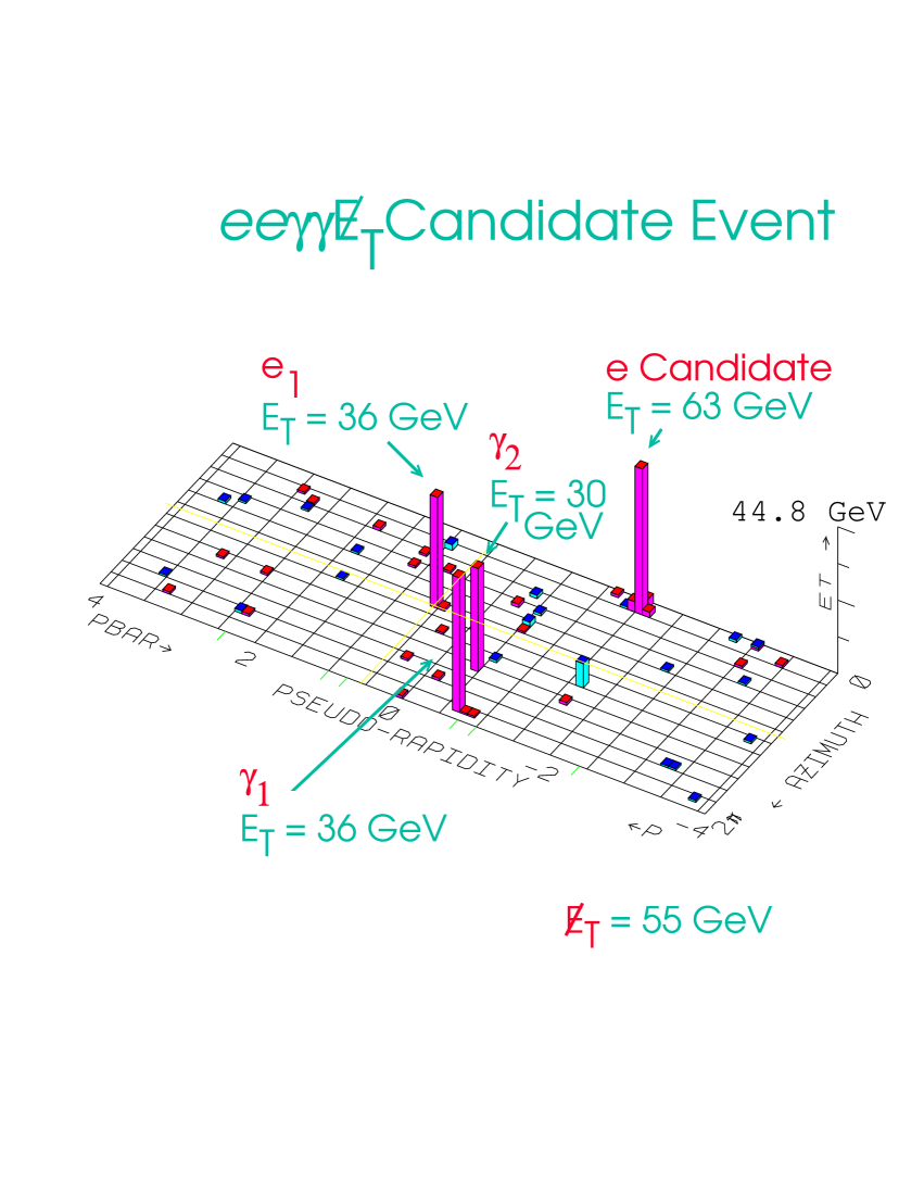
Figure 1.2: The Run I $ee\gamma\gamma\mbox{${\rm\not\!E}_{\rm T}$}$ candidate event.

This signature is predicted to be very rare in the Standard Model of particle physics, with the dominant contribution being from the WW$\gamma\gamma$ production: $WW\gamma\gamma\kern-1.79993pt\rightarrow\kern-1.79993pt(e\nu)(e\nu)\gamma\gamma\kern-1.79993pt\rightarrow\kern-1.79993ptee\gamma\gamma\mbox{${\rm\not\!E}_{\rm T}$}$, from which we expect 8$\times$10^-7 events. All other sources (mostly due to detector misidentification) lead to 5$\times 10^{-7}$ events. Therefore, we expect (1 $\pm$ 1) $\times$ 10^-6 events, which would give us one $ee\gamma\gamma\mbox{${\rm\not\!E}_{\rm T}$}$ candidate event if we have taken one million times more data than we actually had in Run I.

The event raised theoretical interest, however, as the two-lepton two-photon signature is expected in some models of physics ‘beyond the Standard Model’ [1] such as gauge-mediated models of supersymmetry [19, 25].

1.4.2 $\gamma\gamma$+X Search

The detection of this single event led to the development of ‘signature-based’ inclusive searches in Run I to cast a wider net: in this case one searches for two photons + X  [31, 32, 28], where X stands for anything, with the idea that if pairs of new particles were being created these inclusive signatures would be sensitive to a range of decay modes or the creation and decay of different particle types.

In Run I Searches for $\gamma\gamma$+X, all results were consistent with the SM background expectations with no other exceptions other than observation of $ee\gamma\gamma\mbox{${\rm\not\!E}_{\rm T}$}$ candidate event(Table 1.1) [32].

Signature (Object)	Obs.	Expected
${\rm\not\!E}_{\rm T}>35$ GeV, $|\Delta\phi_{\mbox{\scriptsize${\rm\not\!E}_{\rm T}$}-{\rm jet}}|>10^{\circ}$	1	0.5 $\pm$ 0.1
N${}_{\rm jet}\geq 4$, ${\rm E}_{\rm T}^{\rm jet}>10$ GeV, $|\eta^{\rm jet}|<2.0$	2	1.6 $\pm$ 0.4
$b$-tag, ${\rm E}_{\rm T}^{b}>25$ GeV	2	1.3 $\pm$ 0.7
Central $\gamma$, ${\rm E}_{\rm T}^{\gamma_{3}}>25$ GeV	0	0.1 $\pm$ 0.1
Central $e$ or $\mu$, ${\rm E}_{\rm T}^{e~{}{\rm or}~{}\mu}>25$ GeV	3	0.3 $\pm$ 0.1
Central $\tau$, ${\rm E}_{\rm T}^{\tau}>25$ GeV	1	0.2 $\pm$ 0.1

Table 1.1: Number of observed and expected $\gamma\gamma$ events with additional objects in 85 pb^-1[32]

1.4.3 From $\gamma\gamma$ to $\ell\gamma$: $\ell\gamma+X$ Search

Another ‘signature-based’ inclusive search, motivated by $ee\gamma\gamma\mbox{${\rm\not\!E}_{\rm T}$}$ event was for one photon plus one lepton + X [2, 3, 29]. In general data agrees with expectations, with the exception for the $\ell\gamma\mbox{${\rm\not\!E}_{\rm T}$}$ category. We have observed 16 $\ell\gamma\mbox{${\rm\not\!E}_{\rm T}$}$ events on a background of 7.6 $\pm$ 0.7 expected. The 16 $\ell\gamma\mbox{${\rm\not\!E}_{\rm T}$}$ events consist of 11 $\mu\gamma\mbox{${\rm\not\!E}_{\rm T}$}$ events and 5 $e\gamma\mbox{${\rm\not\!E}_{\rm T}$}$ events, versus expectations of 4.2$\pm$0.5 and 3.4$\pm$0.3 events, respectively. The SM prediction yields the observed rate of $\ell\gamma\mbox{${\rm\not\!E}_{\rm T}$}$ with 0.7% probability (which is equivalent to 2.7 standard deviations for a Gaussian distribution). One of the first SUSY interpretation of the CDF $\mu\gamma\mbox{${\rm\not\!E}_{\rm T}$}$ events [19] was resonant smuon $\tilde{\mu}$ production with a single dominant R-parity violating coupling(Figure 1.1).

Category	$\mu_{SM}$	$N_{0}$	P($N\geq N_{0}|\mu_{SM}$), %
All $\ell\gamma X$	–	77	–
Z-like $e\gamma$	–	17	–
Two-Body $\ell\gamma X$	24.9$\pm$2.4	33	9.3
Multi-Body $\ell\gamma X$	20.2$\pm$1.7	27	10.0
Multi-Body $\ell\ell\gamma X$	5.8 $\pm$ 0.6	5	68.0
Multi-Body $\ell\gamma\gamma X$	0.02$\pm$0.02	1	1.5
Multi-Body $\ell\gamma\mbox{${\rm\not\!E}_{\rm T}$}X$	7.6 $\pm$ 0.7	16	0.7

Table 1.2: Run I Photon-Lepton Results: Number of observed and expected $\ell\gamma$ events with additional objects in 85 pb^-1[3]

The Run I search was initiated by an anomaly in the data itself, and as such the 2.7 sigma excess above the SM expectations must be viewed taking into account the number of such channels that a fluctuation could have occurred in. The Run I paper concluded: “However, an excess of events with 0.7% likelihood (equivalent to 2.7 standard deviations for a Gaussian distribution) in one subsample among the five studied is an interesting result, but it is not a compelling observation of new physics. We look forward to more data in the upcoming run of the Fermilab Tevatron.” [3].

Chapter 2 The CDF Experiment at the Tevatron Collider

An important part of the study of elementary particle physics is to understand experimental tools - the accelerators, beams and detectors by means of which particles are accelerated, their trajectories controlled and their collisions studied.

The Tevatron is currently the world’s highest energy particle accelerator. Protons(p) and anti-protons ($\rm{\bar{p}}$) are accelerated to be brought into collision with a center of mass energy of 1.96 TeV. Two detectors are situated at the B$\O$ and D$\O$ collision points, the Collider Detector at Fermilab (CDF) and D$\O$.

2.1 The Tevatron

Figure 2.1: Layout of the Fermilab accelerator complex. Protons (solid arrow) are accelerated at the Cockcroft-Walton, Linac, Booster, Main Injector and finally at the Tevatron. The anti-protons (dashed arrow) from the anti-proton source are first accelerated at the Main Injector and then at the Tevatron.

Fermilab uses a series of accelerators to create the world’s most energetic particle beams. The diagram in Figure 2.1 shows the paths taken by p and $\rm{\bar{p}}$ from initial acceleration to collision in the Tevatron. In the first stage of acceleration H^- ions are created from the ionization of the hydrogen gas and accelerated to a kinetic energy of 750 KeV in the Cockcroft-Walton pre-accelerator [33]. The H^- ions enter a linear accelerator (Linac) [34], where they are accelerated to 400 MeV. The acceleration in the Linac is done by a series of “kicks” from Radio Frequency (RF) cavities. The oscillating electric field of the RF cavities groups the ions into bunches. Before entering the next stage, a carbon foil removes the electrons from the H^- ions at injection, leaving only the protons. The 400 MeV protons are then injected into the circular synchrotron (“Booster”). The protons travel around the Booster to a final energy of 8 GeV.

Protons are then extracted from the Booster into the Main Injector  [35], where they are accelerated from 8 GeV to 150 GeV before the injection into the Tevatron. The Main Injector also produces 120 GeV protons. These protons are extracted and collide with a nickel target, producing a wide spectrum of secondary particles, including $\rm{\bar{p}}$. In the collisions, about 20 $\rm{\bar{p}}$ are produced per one million protons. The $\rm{\bar{p}}$ are collected, focused, and then stored in the Accumulator ring. Once a sufficient number of $\rm{\bar{p}}$ are collected, they are sent to the Main Injector and accelerated to 150 GeV.

Finally, both the p and $\rm{\bar{p}}$ are injected into the Tevatron. The Tevatron, the last stage of Fermilab’s accelerator chain, receives 150 GeV p and $\rm{\bar{p}}$ from the Main Injector and accelerates them to 980 GeV. The p and $\rm{\bar{p}}$ travel around the Tevatron in opposite directions. The beams are brought to collision at the center of the two detectors, CDF II and D$\O$ II (see Figure 2.1).

2.2 The CDF Detector

A discovery will rely heavily on a thorough understanding of the detector. Two aspects are critical: the identification of objects that make up each signature, and the understanding of the calibration and resolution of the detector. The objects for which we have a good understanding of the efficiencies and fake-rates are those for which tracking is essential: electrons, muons, and photons (i.e. a high confidence of the absence of a track), all in the central region. Similarly, the energy scale and resolutions of the calorimeters are well understood in the central region, where the magnetic spectrometer is used to calibrate the calorimeters.

The CDF II detector is a cylindrically-symmetric spectrometer designed to study $\rm p{\bar{p}}$ collisions at the Fermilab Tevatron based on the same solenoidal magnet and central calorimeters as the CDF I detector [36]. A cross-section of one half of the detector is shown in Figure 2.2.

Figure 2.2: Cross-section r-z view of the CDF (see Section 2.2.1).

Because the analysis described here is intended to repeat the Run I search as closely as possible, we note especially the differences from the CDF I detector relevant to the detection of leptons, photons, and ${\rm\not\!E}_{\rm T}$. The tracking systems (Section 2.2.2) used to measure the momenta of charged particles have been replaced with a central outer tracker (COT) that has smaller drift cells [37], and an enhanced system of silicon microstrip detectors [38]. The calorimeters in the regions (Section 2.2.1) with pseudorapidity $|\eta|>1$ have been replaced with a more compact scintillator-based design, retaining the projective geometry (Section 2.2.3). The coverage in $\varphi$ of the central upgrade muon detector (CMP) and central extension muon detector (CMX) systems (Section 2.2.4) has been extended; the central muon detector (CMU) system is unchanged.

The main upgrades to the CDF detector from Run I to Run II, relevant to the analysis, can be summarized as follows:

• Fully digital DAQ system designed for 132 ns bunch crossing times

• Significantly upgraded silicon detector:

  – 707,000 channels compared with 46,000 in Run I

  – Axial, stereo, and 90^∘ strip readout

  – Full coverage over the luminous region along the beam axis

  – Radial coverage from 1.35 to 28 cm for $|\eta|<2$

  – Innermost silicon layer(“L00”) on the beampipe with 6 $\mu$m axial hit resolution

• Outer drift chamber capable of 132 ns maximum drift

  – 30,240 sense wires, 44-132 cm radius, 96 d$E$/d$x$ samples possible per track

• Fast scintillator-based calorimetry out to $|\eta|\simeq 3$

• Expanded muon coverage

• Improved trigger capabilities

  – Drift chamber tracks with high precision at Level-1

  – Silicon tracks for detached vertex triggers at Level-2

• Expanded particle identification via time-of-flight and d$E$/d$x$

2.2.1 CDF Coordinate System

The CDF detector uses a right-handed coordinate system. The horizontal direction pointing out of the ring of the Tevatron is the positive $x$-axis. The vertical direction pointing upwards is the positive $y$-axis. The proton beam direction, pointing to the east, is the positive $z$-axis.

A spherical coordinate system is also used. The radius $r$ is measured from the center of the beamline. The polar angle $\theta$ is taken from the positive $z$-axis. The azimuthal angle $\varphi$ is taken counter-clockwise from the positive $x$-axis.

At a $p\bar{p}$ collider, the production of any process starts from a parton-parton interaction which has an unknown boost along the $z$-axis, but no significant momentum in the plane perpendicular to the $z$-axis, i.e. the transverse plane. This makes the transverse plane an important plane in a $p\bar{p}$ collision. Momentum conservation requires the vector sum of the transverse energy and momentum of all of the final particles to be zero. The transverse energy ${\rm E}_{\rm T}$ and transverse momentum ${\rm p}_{\rm T}$ for a particle produced in a $\rm p{\bar{p}}$ collision are defined by ${\rm E}_{\rm T}=E\times\sin\theta$ and ${\rm p}_{\rm T}=p\times\sin\theta$. We use the convention that “momentum” refers to $pc$ and “mass” to $mc^{2}$.

Another quantity invariant under Lorentz boosts along the beamline is Rapidity, which is defined as $y={{1}\over{2}}log({{E+P_{L}}\over{E-P_{L}}})$, where $P_{L}$ is the longitudinal momentum along the beamline and E is the energy.

Pseudorapidity $\eta$ is used by high energy physicists and is defined as $\eta=-\ln\tan\frac{\theta}{2}$. For massless particles $\eta\equiv y$.

Hard $p\bar{p}$ head-on collisions produce significant momentum in the transverse plane. The CDF detector has been optimized to measure these events. Typically, particles in a $p\bar{p}$ collision event tend to be more in the forward and backward regions than in the central region because there is usually a boost along the $z$-axis. The derivative of $\eta$ is $d\eta=-\frac{d\theta}{\sin\theta}$.

A constant $\eta$ slice corresponds to variant $\theta$ slice which is smaller in the forward and backward regions than in the central region. This makes the $\eta$ occupancy more uniform than $\theta$ occupancy. Therefore, for example, calorimeters are constructed in $\eta$ slices instead of $\theta$ slices.

2.2.2 Tracking

The CDF detector features excellent charged particle tracking and good electron and muon identification in the central region. The detector is built around a 3 m diameter, 5 m long superconducting solenoid operated at 1.4 T. The tracking volume is surrounded by the solenoid magnet and the endplug calorimeters as shown in Figure 2.3.

The CDF tracking system includes a central outer drift chamber (COT) and the silicon tracker. The main parameters of the CDF tracking system are summarized in Table 2.1.

COT
Radial coverage	44 to 132 cm
Number of superlayers	8
Measurements per superlayer	12
Maximum drift distance	0.88 cm
Resolution per measurement	180 $\mu$m
Rapidity coverage	$|\eta|\leq 1.0$
Number of channels	30,240
Layer 00
Radial coverage	1.35 to 1.65 cm
Resolution per measurement	6 $\mu$m (axial)
Number of channels	13,824
SVX II
Radial coverage	2.4 to 10.7 cm, staggered quadrants
Number of layers	5
Resolution per measurement	12 $\mu$m (axial)
Total length	96.0 cm
Rapidity coverage	$|\eta|\leq 2.0$
Number of channels	423,900
ISL
Radial coverage	20 to 28 cm
Number of layers	one for $|\eta|<1$; two for $1<|\eta|<2$
Resolution per measurement	16 $\mu$m (axial)
Total length	174 cm
Rapidity coverage	$|\eta|\leq 1.9$
Number of channels	268,800

Table 2.1: Design parameters of the CDF tracking systems

Figure 2.3: CDF II tracking volume.

The Silicon Tracker

Enhanced system of silicon microstrip detectors [38] consists of three components: Layer 00, the Silicon VerteX detector II (SVX II), and the Intermediate Silicon Layers (ISL). $r-\phi$ view of the silicon tracker is shown in Figure 2.5.

A single layer rad-hard Layer 00 detector is mounted on and supported by the beam pipe. The Layer 00 single-sided sensors provide 6 $\mu$m axial hit resolution.

The next five layers compose the SVX II and are double-sided detectors. The axial side of each layer is used for $r$-$\phi$ measurements. The stereo side of each layer is used for $r$-$z$ measurements.

The two outer layers compose the ISL and are double-sided detectors. This entire system allows charged particle track reconstruction in three dimensions. The impact parameter resolution of SVX II + ISL is 40 $\mu$m including 30 $\mu$m contribution from the beamline. The $z_{0}$ resolution of SVX II + ISL is 70 $\mu$m. The main parameters of the silicon tracker are summarized in Table 2.1.

Figure 2.4: Silicon system.

Figure 2.5: COT superlayers.

The Central Outer Tracker (COT)

The COT [37] is a multi-wire open-cell drift chamber for charged particle reconstruction, occupying the radial region from 44 to 132 cm and $|z|<$155 cm. The COT replaced the Central Tracking Chamber (CTC), which, in addition to aging problems observed during Run I, would also suffer from degraded performance at ${\cal L}\geq 1\times 10^{32}cm^{-2}s^{-1}$. The major problem with the CTC would be its maximum drift time (800 ns) relative to the expected bunch crossing time in Run II (132 ns).

To address this, the COT uses small drift cells ($\sim$2 cm wide, a factor of 4 smaller than the CTC) and a fast gas to limit drift times to less than 130 ns. Each cell consists of 12 sense wires oriented in a plane, tilted with respect to the radial (Figure 2.5). A group of such cells at a given radius is called a superlayer. There are eight alternating superlayers (Figure 2.5) of stereo (nominal angle of 2^∘, used for $r$-$z$ measurement) and axial (used for $r$-$\phi$ measurement) wire planes. The main parameters of the COT are summarized in Table 2.1.

The COT is filled with a mixture of Argon:Ethane = 50:50 which determines the drift velocity. A charged particle travels through the gas mixture and produces ionization electrons. The electrons drift toward the sense wires in the electric field created by cathode field panels and potential wires of the cell. In the crossed magnetic and electric fields electrons originally at rest move in the plane perpendicular to the magnetic field at an angle $\alpha$ with respect to the electric field lines. The value of $\alpha$ depends on the magnitude of both magnetic and electric fields and the properties of the gas mixture. In the COT $\alpha\approx 35^{\circ}$.

The optimal situation for the resolution is when the drift direction is perpendicular to that of the track, which is true for high ${\rm p}_{\rm T}$ tracks because they are almost radial. To make the ionization electrons drift in the $\phi$ direction all COT cells are tilted by 35^∘ with respect to the radial.

When an electron gets near a sense wire the local 1/r field accelerates them causing more ionization and thus forms an ”avalanche” producing a signal (hit) on the sense wire. By measuring the arrival time of “first” electrons (drift time) at sense wire relative to collision time, the distance of the hit is calculated.

COT tracks above 1.5 GeV are available for triggering at Level 1 (XFT tracks). SVX layers 0-3 are combined with XFT tracks at Level-2 (SVT tracks) (see Section 2.2.7 for the description of CDF Run II trigger system).

2.2.3 Calorimetry

The energy measurement is done by sampling calorimeters, which are absorber and sampling scintillator sandwiches with phototube readout. Outside the solenoid, Pb-scintillator electromagnetic (EM) and Fe-scintillator hadronic (HAD) calorimeters cover the range $|\eta|<3.6$. The central calorimeter systems have been retained from Run I, but the plug calorimeters are new detectors for Run II.

Both the central ($|\eta|<1.1$) and plug ($1.1<|\eta|<3.6$) electromagnetic calorimeters have fine grained shower profile detectors at electron shower maximum, and preshower pulse height detectors at approximately $1X_{o}$ depth. Electron identification is accomplished using $E/p$ from the EM calorimeter; using $HAD/EM\sim 0$; and using shower shape and position matching in the shower max detectors. The calorimeter cell segmentation is summarized in Table 2.2 and shown in Figure 3.5. A comparison of the central and plug calorimeters is given in Table 2.3.

$|\eta|$ Range	$\Delta\phi$	$\Delta\eta$
0. - 1.1 (1.2 h)	$15^{\circ}$	$\sim 0.1$
1.1 (1.2 h) - 1.8	$7.5^{\circ}$	$\sim 0.1$
1.8 - 2.1	$7.5^{\circ}$	$\sim 0.16$
2.1 - 3.64	$15^{\circ}$	0.2 $-$ 0.6

Table 2.2: CDF II Calorimeter Segmentation

The region 0.77 $<\eta<$ 1.0, 75 ${}^{\circ}<\phi<$ 90^∘ is uninstrumented to allow for cryogenic utilities servicing the solenoid.

	Central	Plug
EM:
Thickness	$19X_{0},1\lambda$	$21X_{0},1\lambda$
Sample (Pb)	$0.6X_{0}$	$0.8X_{0}$
Sample (scint.)	5 mm	4.5 mm
Stoch. res.	$14\%/\sqrt{E_{T}}$	$16\%/\sqrt{E}$
Shower Max. seg. (cm)	1.4$\phi\times$(1.6-2.0) Z	$0.5\times 0.5$ UV
Hadron:
Thickness	$4.5\lambda$	$7\lambda$
Sample (Fe)	1 to 2 in.	2 in.
Sample (scint.)	10 mm	6 mm

Table 2.3: Central and Plug Upgraded Calorimeter Comparison

Any high energy electron or photon passing through the electromagnetic calorimeters, will undergo pair production ($\gamma\rightarrow e^{+}e^{-}$) and bremsstrahlung ($e^{\pm}\rightarrow\gamma e^{\pm}$) thus producing an electromagnetic shower. The point at which the electromagnetic shower consists of the largest amount of particles is known as the shower maximum. At this point the average energy per particle becomes low enough to prevent further multiplication. After the shower maximum, the shower decays slowly through ionization losses for the electrons and positrons or by Compton scattering for the photons. The calorimeters measure the energy deposited by these showers, and hence the energy of the incident particle. Electromagnetic calorimeters are designed to fully contain showers from electrons and photons.

Hadrons lose energy by nuclear interaction cascades which can have pions, protons, kaons, neutrons, neutrinos, muons, photons, etc. This is significantly more complicated than an electromagnetic cascade and thus results in a large fluctuation in energy measurement.

Central Calorimeters

The central calorimeters consist of the central electromagnetic calorimeter (CEM) [39], the central hadronic calorimeter (CHA) [40], and the end wall hadronic calorimeter (WHA).

The CEM and CHA are constructed in wedges which span 15^∘ in azimuth and extend about 250 cm in the positive and negative $z$ direction, shown in Figure 2.9. There are thus 24 wedges on both the $+z$ and $-z$ sides of the detector, for a total of 48. A wedge contains ten towers, each of which covers a range 0.11 in pseudorapidity. Thus each tower subtends $0.11\times 15^{\circ}$ in $\eta\times\phi$. The CEM covers $0<|\eta|<1.1$, the CHA covers $0<|\eta|<0.9$, and the WHA covers $0.7<|\eta|<1.3$.

The CEM uses lead sheets interspersed with polysterene scintillator as the active medium and employs phototube readout, approximately 19$X_{0}$ in depth, and has an energy resolution of $13.5\%/\sqrt{{\rm E}_{\rm T}}\oplus 2\%$.

To provide more accurate information on the position of the electromagnetic shower inside the calorimeter, the Central Electromagnetic Shower (CES) [39] detector is embedded inside the CEM at the shower maximum, at a depth of approximately 6 radiation lengths. The CES detector is a proportional strip and wire chamber situated at a radius of 184 cm from the beamline. In the azimuthal direction, cathode strips are used to provide the z position and in the $\phi$ direction, anode wires are used. These wires can effectively measure the transverse shower profile to distinguish between a single shower from a prompt photon and two showers from a decay of a neutral meson to two photons, e.g. $\pi^{0}\rightarrow\gamma\gamma$, with a position resolution of 2 mm at 50 GeV.

In order to help particle identification, specifically between electromagnetic and hadronic showers the central preradiator detector (CPR) is mounted on the front of the calorimeter wedges, at a radius of 168 cm from the beamline, and uses the solenoid and tracking detectors as a radiator. It uses proportional chambers to sample the early development of the shower to measure conversions in the coil, helping to distinguish prompt photons and electrons from photons originating from $\pi^{0}$ decays and electrons from conversions. A prompt photon has a 60% probability of converting, while the conversion probability of at least one photon from $\pi^{0}\rightarrow\gamma\gamma$ is about 80% [41].

The CHA and WHA use steel absorber interspersed with acrylic scintillator as the active medium. They are approximately 4.5$\lambda$ in depth, and have an energy resolution of $75\%/\sqrt{{\rm E}_{\rm T}}\oplus 3\%$, as measured on the test beam for single pions [40].

Plug Calorimeters

The plug calorimeters consist of the plug electromagnetic calorimeter (PEM) [42], and the plug hadronic calorimeter (PHA). At approximately 6$X_{0}$ in depth in PEM is the plug shower maximum detector (PES). Figure 2.9 shows the layout of the detector and coverage in polar angle $36.8^{\circ}>\theta>3^{\circ}$ ($1.1<|\eta|<3.64$). Each plug wedge spans 15^∘ in azimuth, however in the range $36.8^{\circ}>\theta>13.8^{\circ}$ ($1.1<|\eta|<2.11$) the segmentation in azimuth is doubled and each tower spans only 7.5^∘.

The PEM is a lead-scintillator sampling calorimeter. It is approximately 21$X_{0}$ in depth, and has an energy resolution of $16\%/\sqrt{E}\oplus 1\%$. The PES consists of two layers of scintillating strips: U and V layers offset from the radial direction by $+22.5^{\circ}$ and $-22.5^{\circ}$ respectively, as shown in Figure 2.9. The position resolution of the PES is about 1 mm. The PHA is a steel-scintillator sampling calorimeter. It is approximately 7$\lambda$ in depth, and has an energy resolution of $74\%/\sqrt{E}\oplus 4\%$, as measured on the test beam for single pions [40].

Figure 2.6: CEM/CES/CHA wedge.

Figure 2.7: CES strip and wire.

Figure 2.8: PEM/PES/PHA layout.

Figure 2.9: PES U and V layers.

2.2.4 Muon Systems

The muon is a minimum ionizing particle which loses very little energy in detector materials. The muon’s lifetime, 2.2 $\mu$s, is long enough for the muon to pass through all the detector components, reach the muon chambers and decay outside.

There are four independent muon systems: the central muon detector (CMU) [43], the central muon upgrade (CMP) [44], the central muon extension (CMX) [45], and the intermediate muon detector (IMU). The calorimeter steel serves as a filter for muon detection in the CMU and CMX, over the range $|\eta|<1$, $p_{T}>1.4$ GeV. Additional iron shielding, including the magnet yoke, provides a muon filter for the CMP in the range $|\eta|<0.6$, $p_{T}>2.2$ GeV. The (non-energized) forward toroids from Run I provide muon filters for IMU in the range $1.0<|\eta|<1.5$ for $p_{T}>2$ GeV. Scintillators for triggering are included in CMP, CMX, and IMU.

Muon identification is accomplished by matching track segments in the muon chambers with COT/SVX tracks; matching is available in $r-\phi$ for all detectors and in $z$ in CMU and CMX. The parameters for the muon systems are summarized in Table 2.4. The IMU, which provides coverage in the forward region will not be discussed in detail, as it is not used for this analysis.

The coverage for the muon systems in $\eta-\phi$ space is shown in Figure 2.12. CMU, CMP and CMX muon systems are also shown in Figure 3.6.

	CMU	CMP	CMX	IMU
Pseudo-rapidity coverage	$|\eta|\leq 0.6$	$|\eta|\leq 0.6$	$0.6\leq|\eta|\leq 1.0$	$1.0\leq|\eta|\leq 1.5$
Drift tubes
Cross-section, cm	2.68 x 6.35	2.5 x 15	2.5 x 15	2.5 x 8.4
Length, cm	226	640	180	363
Max drift time, $\mu{\rm s}$	0.8	1.4	1.4	0.8
Scintillation counters
Thickness, cm		2.5	1.5	2.5
Width , cm		30	30-40	17
Length , cm		320	180	180
Minimum muon $p_{T}$,  GeV	1.4	2.2	1.4	1.4-2.0

Table 2.4: Design Parameters of the CDF II Muon Detectors.

A muon chamber contains a stacked array of drift tubes and operates with a gas mixture of Argon:Ethane = 50:50. The basic drift principle is the same as that of the COT, but the COT is a multi-wire chamber, whereas at the center of a muon drift tube there is only a single sense wire. The sense wire is connected to a positive high voltage (HV) while the wall of the tube is connected to a negative HV to produce a roughly uniform time-to-distance relationship throughout the tube. The drift time of a single hit gives the distance to the sense wire, and the charge division at each end of a sense wire can in principle be used to measure the longitudinal coordinate along the sense wire. The hits in the muon chamber are linked together to form a short track segment called a muon stub (Figure 2.10). If a muon stub is matched to an extrapolated track in the tracking system (Section 2.2.2), a muon is reconstructed.

Figure 2.10: A CMU module in the r-$\phi$ plane with 4 layers of drift chambers. The drift times t1 and t2 are used to calculate muon momentum for triggering (Section 2.2.7). The sense wires connected to the readout are shown as a black circles.

Figure 2.11: Location of the muon detectors in $\phi$ and $\eta$. On the east side, there is a gap in coverage in the CMX of 30^∘ in azimuth, due to the location of the cryogenic utilities servicing the solenoid.

Figure 2.12: Central muon systems: CMU, CMP, CMX.

CMU and CMP

The CMU is unchanged from Run I. It is located behind the towers of the CHA and divided into wedges covering 12.6^∘ in azimuth for $\eta<$ 0.6. Only muons with a ${\rm p}_{\rm T}>$ 1.4 GeV reach the CMU. Each wedge has three towers, each comprised of four layers of four drift tubes. The second and fourth layers are offset by 2 mm in $\phi$ direction from the first and third as shown in Figure 2.10. Six CMU wedges and their relative location with respect to CMX and CMP (outer box) subsystems are shown in Figure 2.12.

A 50 $\mu$m diameter stainless steel resistive sense wire is located in the center of each cell. The wires in the cells in the first and third (second and fourth) layers are connected in the readout. Each wire pair is instrumented with a time-to-digital converter (TDC) to measure the $\phi$-position of the muon and an analogue-to-digital converter (ADC) on each end to measure z position via charge division. The position resolution of the detector is 250 $\mu$m in the drift direction (r-$\phi$) and 1.2 mm in the sense wire direction (z).

Approximately 0.5% of high energy hadrons produced will pass through the CMU creating an irreducible fake muon background. In order to reduce this effect, an additional muon chamber (CMP) is installed behind 60 cm of steel.

The CMP consists of a four-sided box placed on the outside of the CDF detector. Muons with ${\rm p}_{\rm T}>$ 2.2 GeV can reach the CMP. The rectangular form of the CMP detector means that its $\eta$ varies in azimuth (Figure 2.12). The CMP covers $|\eta|<0.6$.

The maximum drift time of the CMU is longer than the $\rm p{\bar{p}}$ bunch crossing separation, which can cause an ambiguity in the Level 1 trigger (Section 2.2.7). To resolve the ambiguity scintillation counters are used. The scintillation counters (CSP) are installed on the outer surface of the CMP.

Central Muon Extension (CMX)

The CMX has eight layers and extends the $\eta$ coverage to $0.6<|\eta|<1.0$. It consists of two 120^∘ arches located at each end of the central detector, as shown in Figure 2.12. The uninstrumented regions have been filled by the insertion of a 30^∘ keystone at the top, and two 90^∘ miniskirts for the lower gaps. There is a gap in the coverage on the east side due to cryogenic utilities servicing the solenoid as shown in Figure 2.12, known as the ”chimney”.

A layer of scintillation counters (the CSX) is installed on both the inside and the outside surfaces of the CMX. No additional steel was added for this detector because the large angle through the hadron calorimeter, magnet yoke, and steel of the detector end support structure provides more absorber material than in the central muon detectors.

2.2.5 Time of Flight System

The Time of Flight detector (TOF) [46] measures the time taken by a particle to travel from the interaction point to the detector, and has a particle timing resolution of 100 ps. This information can be used to differentiate between different particle types (e.g. kaons, pions) and also to help tag cosmic ray events.

The TOF is situated between the COT and the solenoid. It consists of 216 scintillator bars with dimensions 4$\times$4$\times$276 cm. At each end of the scintillator bars a photomultiplier tube is mounted

2.2.6 Cherenkov Luminosity Counters

Luminosity (${\cal L}$) is a measure of particle interaction, specifically the chance that a proton will collide with an antiproton. The rate of inelastic scattering in $\rm p{\bar{p}}$ interactions can be used to determine the ${\cal L}$ .

A gas Cherenkov Luminosity Counter (CLC) [47] measures the number of interactions per beam crossing to determine the luminosity of the Tevatron. There are two CLCs positioned between the beam-pipe and the plug calorimeters, covering the region 3.7 $<|\eta|<$ 4.7. Each CLC consists of 48 thin, conical gas-filled Cherenkov counters. They are arranged in three concentric circles, each consisting of 16 counters (see, for example, Figure 3.7).

The luminosity of a $\rm p{\bar{p}}$ collider can be estimated using the equation:

$${\cal L}={{f\times\mu}\over{\sigma}}$$ (2.1)

where f is the frequency of bunch crossing, $\mu$ is the average number of interactions per beam crossing, given by the CLC hit rate (about 5-6), and $\sigma$ is the inelastic cross-section of $\rm p{\bar{p}}$ scattering. The average of the inelastic cross-sections as measured by CDF Run I and the E811 [48] is 60.7$\pm$2.3 mb [49].

A total systematic uncertainty of 6% is quoted for all luminosity measurements. This includes a 4.4% contribution from the acceptance and operation of the luminosity monitor and 4.0% from the theoretical uncertainty on the calculation of the total $\rm p{\bar{p}}$ cross-section [49].

2.2.7 Trigger and Data Acquisition

Many interesting physics processes have cross sections which are many orders of magnitude smaller than the total inelastic cross section. The collision rate at the Tevatron is much higher than the rate at which data can be recorded. Therefore, the trigger needs to be fast and accurate to record as many interesting events as possible, while rejecting uninteresting events.

To accomplish this, the CDF trigger system has a three-level architecture: Level 1 (L1), Level 2 (L2), and Level 3 (L3). The data volume is reduced at each level, which allows more refined filtering at subsequent levels with minimal deadtime. Each sub-detector generates primitives which can be used in the trigger system to select events. The trigger system block diagram is shown in Figure 2.13.

Figure 2.13: Trigger system block diagram: flow of data through L1 and L2 of trigger system. Silicon Vertex Tracker (SVT), based on the track impact parameter of displaced tracks, is used by L2. The data volume is reduced at each level which allows more refined filtering at subsequent levels with minimal deadtime. L3 is purely a software trigger consisting of the event builder running on a large PC farm.

At L1 axial layers of the COT are used by eXtreme Fast Tracker (XFT) to reconstruct $\phi$ and ${\rm p}_{\rm T}$ for the tracks. Based on the XFT tracks and a ratio of the hadronic energy to the electromagnetic energy of a calorimeter tower (HAD/EM ratio) electrons and photons are then reconstructed. Muons are reconstructed by matching XFT and muon hits. Jets are reconstructed based on a sum of the electromagnetic and hadronic energies for a tower. ${\rm\not\!E}_{\rm T}$ and $\sum{\rm E}_{\rm T}$ (a scalar sum of the energies of all of the calorimeter towers) are also reconstructed at L1.

L1 is a synchronous hardware trigger and it makes a decision within 4 $\mu$s. This trigger reduces the event rate from 7.6 MHz to 50 KHz, which is limited by the L2 processing time. Accepted events are then passed to the L2 hardware.

At L2 SVX layers 0-3 are combined with XFT tracks (Figure 2.13.). The L2 uses jet clustering as well as improved momentum resolution for tracks, finer angular matching between muon stubs and central tracks and data from the CES for improved identification of electrons and photons.

The L2 decision time is about 20 $\mu$s. L2 is a combination of hardware and software triggers and is asynchronous. If an event is accepted by L1, the front-end electronics moves the data to one of the four onboard L2 buffers. This is sufficient to process a L1 50 KHz accept rate and to average out the rate fluctuations. The L2 accept rate is about 300 Hz which is limited by the speed of the event builder in L3.

L3 is a purely software trigger consisting of the event builder running on a large PC farm. Data which passes one of the specified trigger paths is reconstructed at L3 using full detector information and the latest calibrations. The L3 accept rate of about 75 Hz is limited by the speed of writing data to tape for the permanent storage.

As soon as an event passes L3 it is delivered to the data-logger subsystem which sends the event out to permanent storage for offline reprocess, and to online monitors which verify that the entire detector and trigger systems are working properly. One of the online monitors, CDF Run II Event Display, is described in detail in Section 3.

Chapter 3 CDF Run II Event Display

Event displays are indispensable tools for data analysis in high energy physics experiments. They help to understand the physics of a recorded interaction, to diagnose the apparatus, to make the detector geometry imaginable and to illustrate the whole matter to general audiences.

CDF Run II Event Display (EVD) [11] is a major contribution to the commissioning and operation of CDF II detector. Development and support of the EVD package [10] is one of the responsibilities of the ITEP(Moscow) group at CDF [13].

The data from the collider experiment is a stream of signals from subdetectors. The detector ”sees” these signals as sequences of impulses, distributed over many channels of different subdetectors (see Section 2.2). The signals are analyzed by powerful pattern recognition and analysis programs, which create more sophisticated objects like clusters, segments, stubs and then tracks, muons, electrons/photons, jets, etc.

Typically physics results are based on statistical analysis of many events. The standard forms of presentation are histograms, graphs and tables. However, a graphical representation of a single event a powerful tool for checking the validity of reconstruction or analysis algorithms. For a quick assessments of error conditions as well as for public presentations the visual representation is the most efficient way to transfer information to a human brain.

Higher event multiplicities and higher momenta of outgoing particles are matched by detectors with a growing number of subunits of increasing granularity, resolution and precision. As a consequence pictures of detectors and events are getting more complicated and may even get incomprehensible. This leads to a question if the presentation of data via visual techniques is useful for complicated events at the Tevatron.

3.1 Overview

The aim of the EVD is to enable visual representation of the objects existing in the CDF Run II software. EVD interacts both with the data and with the simulation and reconstruction packages. For simulated data EVD visualizes the Decay Tree, which is constructed from HEPG information.

It is natural to define three kinds of objects: Real Objects (Section 3.1.1), Graphical Objects (Section 3.1.2), and Views (Section 3.1.3). To visualize Real Objects and to access information about the event, Operations (Section 3.1.4) are performed on the Graphical Objects and Views.

3.1.1 Real Objects

A Real Object is information from a subdetector or combined information from several subdetectors. For example, to identify electron one needs calorimeter and tracking information. Some of the Real Objects in CDF are listed below:

• Tracking information (Section 2.2.2)
  – axial and stereo hits from the COT
  – hits from the silicon tracker
  – tracks reconstructed with different tracking algoritms

• Calorimeter information (Section 2.2.3)
  – Central and Plug Shower Chambers information
  – Central and Plug Preradiator information

• Hits from TOF system (Section 2.2.5)

• Information from the muon systems (Section 2.2.4)
  – Hits from the muon systems
  – Track segments reconstructed in the muon chambers

• Information from East and West CLC subdetectors, which are used to monitor luminosity and to identify diffractive events (Section 2.2.6)

• Information from Beam Shower Counters [50], used to identify diffractive events

• Information from CDF Run II L1/L2/L3 Trigger System (Section 2.2.7)

• EM Timing information [51]

• Pre-reconstructed objects, such as Muon, Electron, Photon, Jet Candidates, ${\rm\not\!E}_{\rm T}$

• Full information about raw and reconstructed data
  – access to banks and collections in the event

A major requirement has been made to keep analysis in the EVD to a minimum, as objects are identified differently in different analyses (i.e. loose electron for one analysis may be a jet in some other analysis). However, EVD has a functionality to clean complicated events by selective presentation of parts of the data and the detector. (Section 3.1.4). For example, EVD can show or hide tracks depending on their properties ($\phi$, $\eta$, ${\rm E}_{\rm T}$, ${\rm p}_{\rm T}$, number of hits in a subsystem etc.).

3.1.2 Graphical Objects

Real Objects in the EVD are mapped to their visual representation into Graphical Objects of different types, corresponding to different Views. The graphical objects correspond to the stored real objects (for example, to the list of hits and tracks) and other real objects (for example, to electron, muon and photon candidates) created from them.

The properties of Real Objects are used to display Graphical Objects. For instance, information from the calorimeter is shown as towers with a size proportional to the deposited energy. We use graphics libraries available in the ROOT package [52].

3.1.3 Views

View is a method of visualizing a set of graphical objects. For a user, view is generally a window with a defined way of displaying Graphical Objects. We define three categories of views for the CDF Run II Event Display:

1. Realistic Views are obtained by either a sequence of rotations, linear scaling, and projections of a geometry of detector/identified objects. Realistic views are understood intuitively, although the pictures may become too complex (for example, see Figures 3.4 and 3.6).

   Hits density as well as detector precision grow towards the interaction point. Therefore, an ability to hide parts of the detector obscuring the picture is crucial. Another feature of the EVD is to show or hide Graphical objects depending on the properties of Real Objects (number of hits, drift time etc.)

2. Schematic Views can be obtained from realistic views by changing the aspect ratio or focal length for a subdetector. For example, the scale may be decreased with increasing radius, so that the inner subdetectors appear enlarged. This emphasizes the commonly used construction principle of detectors, namely that precision and sampling distance decrease, when stepping from the inner to the outer detectors.

   Schematic Views do not necessarily represent the detector in its real proportions or shapes. For example a box that changes color depending on error conditions may serve as a schematic view of any detector component. In many cases the schematic views are relatively easy to understand and very efficient to use (for example, see Figure 3.3).

3. Abstract Views have little resemblance to the detector image in cartesian space. These views are not intuitively understood but given some training may be the most powerful. Examples of abstract views are angular projections, histograms, LEGO plots, etc. (for example, see Figure 3.5)

3.1.4 Operations

Operations on Graphical Objects:
These operations only change the visual properties of the graphical objects, the real objects are not changed. Visual operations can be performed on the graphical objects or on the views. The following operations on graphical objects are supported:

• rotation, zooming, translation, scaling

• viewpoint changing

• object hiding/unhiding

• sub-view creation

• redefinition of visual properties of graphical objects

Operations on Real Objects:
Operations on real objects can access information about the objects or change the state of these objects. In addition, visual properties of the corresponding graphics objects can also be changed as a result of changing real objects. The following operations on real objects are supported:

• access to public member functions for an object from the EVD

• obtaining the detailed information on an object properties (for example, for tracks one can access information on number/type of hits in COT/Silicon detectors, dE/dx, $\chi^{2}$, $d_{0}$, $z_{0}$ etc.)

• access to event record information (data banks and collections)

• application of identification cuts

• interface to a histogramming package

3.2 CDF Run II Application Framework

The design of the EVD is based on the belief that both requirements and graphics software abilities will be very broad at any time and will constantly evolve. The EVD is designed to accommodate that diversity and change. This can be accomplished only by sufficient flexibility and modularity of the core control structure [53].

An application framework, in the context of a high energy physics experiment, is a ”system” that allows physicist-developed code to be combined with code developed by other people and to be used in both the online and offline environments. Either real or simulated data can be used as the input and the output can include (modified) copy of the input as well as additional reconstructed quantities. This output then forms the input in the next stage of a multi-stage data reduction environment. CDF Run II Application Framework (AC++) is based on the ROOT object oriented analysis framework [52], which is incorporated in CDF Run II C++ software.

     

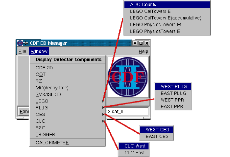
(a) A screen shot of the manager window for the EVD.

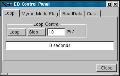
(b) The EVD control panel with the Loop tab selected.

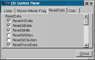
(c) Data Menu to select which data to read.

Figure 3.1: CDF Run II Event Display Graphical User Interface. The start of the EVD is signalled by the appearance of the manager window (a). Clicking the Panel button brings up the EVD control panel (b). The control panel allows you to configure the behavior of the EVD. For example, user may select which data to read using the DataMenu (c).

The AC++ provides a unified framework for event reconstruction, post-production analysis and online monitoring, triggering and calibration. The goals of the framework is to provide a simple and straightforward means of combining any number of independent classes, called modules, into a single executable and to provide a flexible system for specifying (either interactively or in a batch mode) how these modules are run.

Therefore, EVD has the flexibility to enable/disable different modules, so that one can work with unprocessed data for the immediate feedback. Alternatively, one can also run reconstruction modules inside the EVD with user-defined parameters for debugging purposes.

3.3 Graphical User Interface

The start of the EVD is signalled by the appearance of the manager window (Figure 3.1,a). From the manager window user select one of the event displays, and control automatic looping through events, as is done in the CDF Run II control room at $B\O$. The name of the input file is displayed at the bottom.

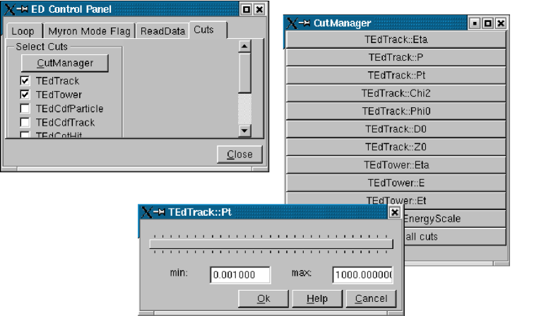
Figure 3.2: Cut Manager. Complicated events might be cleaned by selective presentation of the data. User can specify cuts on physical quantities of the displayed objects, such as the $\eta$, $\phi$, ${\rm p}_{\rm T}$ of tracks or the energies deposited in the calorimeter towers.

Clicking the Panel button brings up the EVD control panel (Figure 3.1, b). The control panel allows user to configure the behavior of the EVD. User may select which data to read using the DataMenu (Figure 3.1, c)

Complicated events might be cleaned by selective presentation of parts of the data and the detector. User can specify cuts on physical quantities of the displayed objects, such as the $\eta$, $\phi$, ${\rm p}_{\rm T}$ of tracks or the energies deposited in the calorimeter towers. This helps to clean up the event by removing low-${\rm p}_{\rm T}$ tracks and low-${\rm E}_{\rm T}$ towers, or to debug reconstruction problems by requiring EVD to show objects which pass some cuts (e.g. number of COT or Silicon hits, or tracks with large $d_{0}$ etc.). Figure 3.2 shows sample Cut Manager session.

3.4 Displays

3.4.1 $r-\phi$ and $r-z$ Views

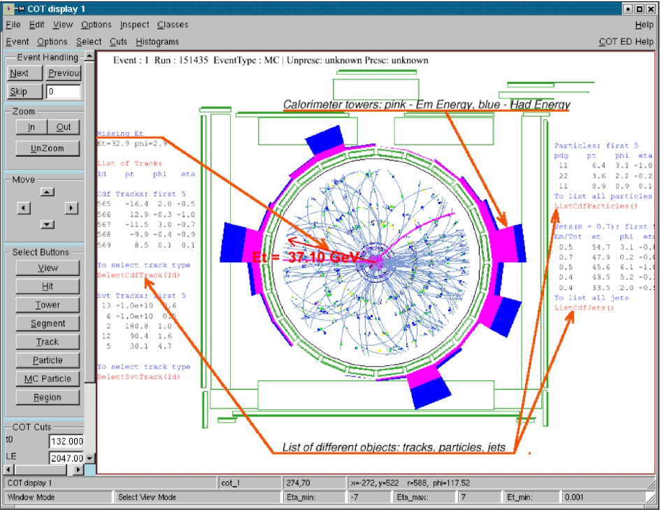
Figure 3.3: COT Display ($r-\phi$ view).

In layered projections, each geometry object acquires a 2-dimensional shape which can be different in each projection. For example, the drift chamber outline is a circle in the $r-\phi$ view and a rectangle in the $r-z$ view.

The $r-\phi$ view (COT Display, Figure 3.3) shows hits in the subdetectors (COT, Silicon trackers, Muon Chambers, TOF, XTRP etc.), energies in the central EM and HAD calorimeter towers (summed over $\eta$), missing ${\rm E}_{\rm T}$ information, information about CDF reconstructed objects, such as $e$, $\mu$, $\gamma$, jet candidates. It also gives the information about run/event number, as well as trigger information.

Figure 3.3 is an example of a schematic view (Section 3.1.3), and it is obtained from a realistic $r-\phi$ projection by applying a fish-eye transformation to a COT volume.

A fish-eye view introduces a nonlinear transformation of radius in the layered $r-\phi$ projection, with the aim to enable simultaneous inspection of tracking chambers, calorimetry and muon system within the same picture (Figure 3.3).

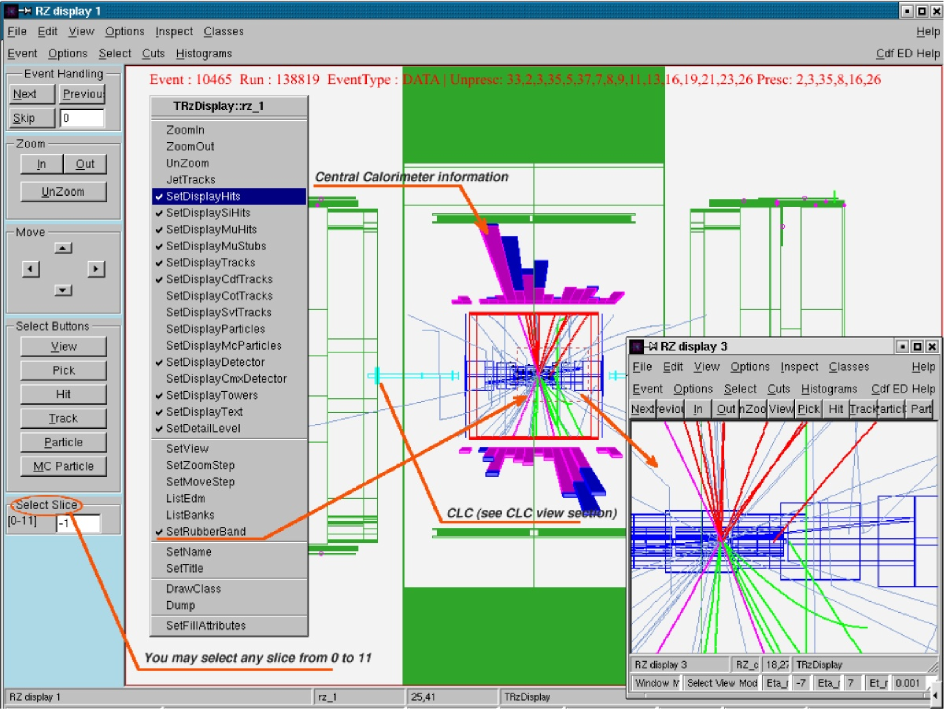
Figure 3.4: RZ Display ($r-z$ view).

The $r-z$ view (Figure 3.4) is designed to show the same information as $r-\phi$ view, but in $r-z$ projection. The only exception are COT hits, which do not have z coordinate and therefore are displayed in $r-\phi$ projection only. Energies in the central EM and HAD calorimeter towers are summed over $\phi$. Figure 3.4 is an example of a realistic view (Section 3.1.3).

User can “slice” the detector by selectin pair of opposite wedges (”Select Slice” option at the bottom of the RZ display menu, Figure 3.4) to reduce the amount of information displayed. In this case one will have only those wedges’ tracks, hits, bits, and calorimeter towers. There are 24 15^∘ wedges, which are displayed in 12 opposite pairs. The default slice value is -1, which folds all upper wedges onto the top and all lower wedges onto the bottom, which is the way the RZ display used to work in CDF Run I.

3.4.2 Lego Displays

These are generic LEGO plot windows (Figure 3.5) showing a variable (E, ${\rm E}_{\rm T}$, ADC counts) as a function of eta-phi. Figure 3.5 is an example of an abstract view (Section 3.1.3). $\eta-\phi$ grid corresponds to $\eta-\phi$ segmentation of CDF calorimeter system (Section 2.2.3); each bin on the lego display represents a tower. Towers corresponding to CDF Run II particle candidates (e, $\mu$, $\gamma$, jets) have been added to LEGO views to improve the display (see Figure 3.5). User can interactively rotate LEGO display/change default settings to obtain a better view of an event.

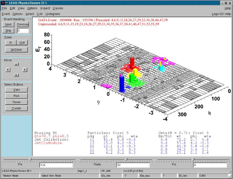
Figure 3.5: The Lego Display shows the variable ${\rm E}_{\rm T}$ as a function of eta-phi.

There also many other LEGO-based views, used to monitor/debug specific subdetectors, such as the PLUG/PPR Views to visualize Plug Calorimeter information, and the CES View to show the sums of energies for CES Strips and Wires. In addition to the views itself there is an interface to a histogramming package to obtain specific distributions. For example, one can see distributions of measurements in strips/wires of the CES. Views are designed to give a general idea about an event, and histograms allow to see more detailed picture for a part of a subdetector.

3.4.3 3D Displays

Perspective 3-dimensional views with hidden lines and hidden surface removal are very useful for understanding detector geometry, and provide attractive pictures for public relation (PR) purposes (Figure 3.6). Analyzing the event itself is often less successful in this mode, since the complicated geometry tends to obscure the tracks and hits.

Figure 3.6 is an example of a realistic view (Section 3.1.3). There are several available 3D views which one can use separately for specific needs or combine to obtain a complicated view.

• CDF 3D display
  – 3-dimensional view of the CDF detector with tracks/silicon hits/muon hits and stubs)

• 3D calorimeter display
  – central and plug calorimeter towers together with tracks

• SVX 3D display
  – dedicated silicon detector display, which shows the silicon hits/strips together with tracks). SVX 3D display is designed to obtain detailed information for all silicon hits associated with a given track, which is helpful for debugging purposes.

Figure 3.6: 3-dimensional OpenGL view of detector geometry with hidden lines removal.

Three-dimensional Views with hidden lines and surface removal are possible through the special OpenGL viewer which is integrated in view. Figure 3.6 has been obtained using OpenGL. In this mode live rotations are possible given a suitable hardware acceleration for the instantaneous response.

3.4.4 Other Displays

There many other views (see Figure 3.7), used to monitor different CDF Run II subsystems and to analyze real and simulated data:

• Wedge Display
  – CES/CPR information together with central calorimeter information

• Trigger Display
  – Level 1, Level 2, Level 3 trigger bits and corresponding names

• BSC Display
  – shows ADC counts from beam shower counter subdetectors

• CLC Display
  – shows ADC counts from Cherenkov Luminosity Counters

• MC Decay Tree Display
  – decay tree constructed from HEPG information for the simulated data

Figure 3.7: CDF ”Live Events” public page.

3.5 Live Events

The Live Events page has been designed to provide attractive pictures for PR purposes [12]. The Views displayed on Figure 3.7 from the top to the bottom are as follows:

• 1st row:
  COT Display. COT Display zoomed to access central outer tracker information. COT Display zoomed to access silicon tracker information

• 2nd row:
  RZ Display. SVX 3D Display. Calorimeter LEGO Display

• 3rd row:
  East Plug LEGO Display. Calorimeter 3D Display. West Plug LEGO Display

• 4th row:
  East CLC Display. BSC Display. West CLC Display

3.6 Conclusions

From the very beginning of Run II data taking EVD is in continuous use for the online monitoring and for the analyses. This answers the question whether a presentation of data via visual techniques is possible for complicated events at the Tevatron. More importantly, features of the EVD make it to be one of the most important tools for a better understanding of the events which could possibly be New Physics candidates in a CDF Run II data.

Chapter 4 $\ell\gamma+X$ Selection

4.1 Datasets

The data presented in the thesis was taken between March 21, 2002, and August 22, 2004 and represent $305pb^{-1}$ for which the silicon detector (Section 2.2.2) [38], and all three central muon systems (CMP, CMU and CMX), described in Section 2.2.4 were operational.

The $\mu\gamma$ candidates are taken from a logical ‘OR’ of the inclusive high-${\rm p}_{\rm T}$ muon sample and the inclusive high-${\rm E}_{\rm T}$ photon sample; this was done to ensure a high and stable trigger efficiency for the muons. For consistency, $e\gamma$ candidates are also obtained from a logical ’OR’ of the inclusive high-${\rm E}_{\rm T}$ electron sample and the inclusive high-${\rm E}_{\rm T}$ photon sample. Each of the samples was ntupled using the UC flat ntuple [54].

To accept an event from the inclusive high-${\rm p}_{\rm T}$ lepton sample we require the event to have a loose lepton and a photon, or two leptons (either tight or loose), or a tight lepton and $\mbox{${\rm\not\!E}_{\rm T}$}>15GeV$ (see Tables 5.1, 6.1, 6.2 and 7.1).

To accept an event from the inclusive high-${\rm p}_{\rm T}$ photon sample we require the event to have a tight photon (see Table 7.1) and a loose lepton. The muon selection criteria are listed in Table 5.1; the electron selection criteria are listed in Tables 6.1 and 6.2;

We check data integrity during the run by plotting the stability of the event yields for the control samples. We use the 8 time intervals defined in Table 4.1 [55]. The boundaries of the intervals have been chosen to correspond to shutdowns or to major changes in the trigger table. The luminosity in each bin is plotted in Figure 4.1.

Run	Table	Date	${\cal L}$, $pb^{-1}$	Comment
141544	PHYSICS_1_01 4_275	2002.03.23		Start
152949	PHYSICS_1_02 7_175_323	2002.10.16	15.8 $\pm$ 0.9	TrigTable
152593	PHYSICS_1_03 1_185_325	2002.10.16		TrigTable
156487	PHYSICS_1_03 2_194_329	2003.01.12	36.8 $\pm$ 2.2	Shutdown
159603	PHYSICS_1_04 4_255_357	2003.02.28		Startup
163113	PHYSICS_1_04 9_288_373	2003.05.19	45.9 $\pm$ 2.8	TrigTable
163130	PHYSICS_1_05 1_290_375	2003.05.19		TrigTable
166325	PHYSICS_1_05 3_298_382	2003.07.18	30.1 $\pm$ 1.8	TrigTable
166328	PHYSICS_1_05 5_319_391	2003.07.18		TrigTable
168889	PHYSICS_1_05 8_345_402	2003.09.06	39.0 $\pm$ 2.3	Shutdown
175066	PHYSICS_1_05 8_345_404	2003.11.26		Startup
179056	PHYSICS_2_01 4_416_424	2004.02.13	42.4 $\pm$ 2.5	COT bad
182843	PHYSICS_2_05 1_475_455	2004.05.19		COT good
184835	PHYSICS_2_05 11_508_473	2004.07.06	41.1 $\pm$ 2.5	TrigTable
184868	PHYSICS_2_05 11_508_473	2004.07.07		TrigTable
186598	PHYSICS_2_05 17_531_484	2004.08.22	50.0 $\pm$ 3.0	Shutdown

Table 4.1: The intervals in run number used to check the stability of W and Z event yields versus time. The boundaries of the intervals have been chosen to correspond to shutdowns or to major changes in the trigger table. The offline luminosity is shown; the luminosity scale factor of 1.019 has not been applied. The systematic error of 6% (Chapter 11) in the ${\cal L}$ is shown.

(a) Luminosity in stability bins, $pb^{-1}$

Figure 4.1: The luminosity in each of the 8 time intervals defined in Table 4.1, used to check the stability of control event yields during the run. The boundaries of the intervals have been chosen to correspond to shutdowns or to major changes in the trigger table. The total luminosity is $305~{}pb^{-1}$. The 6% luminosity uncertainty (Chapter 11) is not shown.

To summarize, in the resulting inclusive electron and muon samples every event contains either a $l\gamma$ candidate, or a candidate for the $W$ and $Z^{0}$ control samples, described in detail below in Chapters 5 and 6.

4.2 Selection Overview

Events with a high transverse momentum (${\rm p}_{\rm T}$) lepton or photon are selected by a three-level trigger [43] that requires an event to have either a lepton with ${\rm p}_{\rm T}>18~{}GeV$ or a photon with ${\rm E}_{\rm T}>25~{}GeV$ within the central region, $|\eta|\lesssim 1.0$. The trigger system selects photon and electron candidates from clusters of energy in the central electromagnetic calorimeter. Electrons are further distinguished from photons by requiring the presence of a COT track pointing at the cluster. The muon trigger requires a COT track that extrapolates to a reconstructed track segment (“stub”) in the muon drift chambers.

We use the same kinematic event selection as in the Run I analysis: inclusive $\ell\gamma$ events are selected by requiring a central photon candidate with $\mathrm{E_{T}^{\gamma}}>25$ $GeV$, a central lepton candidate ($e$ or $\mu$) with $\mathrm{E_{T}^{\ell}}>25$ $GeV$ passing the “tight” criteria listed below, and a point of origin along the beam-line not more than 60 cm from the center of the detector.

A muon candidate (Chapter 5) passing the “tight” cuts has the following properties: a) a well-measured track in the COT; b) energies deposited in the electromagnetic and hadron compartments of the calorimeter consistent with expectations; c) a muon “stub” track in the CMX detector or in both the CMU and CMP detectors [43] consistent with the extrapolated position of the COT track; and d) COT timing measurements consistent with a track from a $\rm p{\bar{p}}$ collision and not from a cosmic ray.

An electron candidate (Chapter 6) passing the “tight” selection has the following properties: a) a high-quality track with ${\rm p}_{\rm T}$ of at least half the shower energy, unless the ${\rm E}_{\rm T}>100$ $GeV$, in which case the ${\rm p}_{\rm T}$ threshold is set to 25 $GeV$; b) a transverse shower profile consistent with an electron shower shape and that matches the extrapolated track position; c) a lateral sharing of energy in the two calorimeter towers containing the electron shower consistent with that expected; and d) minimal leakage into the hadron calorimeter.

Photon candidates (Chapter 7) are required to have no track with ${\rm p}_{\rm T}>1$ $GeV$, and at most one track with ${\rm p}_{\rm T}<1$ $GeV$, pointing at the calorimeter cluster; good profiles in both transverse dimensions at shower maximum; and minimal leakage into the hadron calorimeter.

To reduce background from photons or leptons from the decays of hadrons produced in jets, both the photon and the lepton in each event are required to be “isolated”. The ${\rm E}_{\rm T}$ deposited in the calorimeter towers in a cone in $\eta-\varphi$ space of radius $R=0.4$ around the photon or lepton position is summed, and the ${\rm E}_{\rm T}$ due to the photon or lepton is subtracted. The remaining ${\rm E}_{\rm T}$ in the cone is required to be less than $2.0~{}GeV+0.02\times({\rm E}_{\rm T}-20~{}GeV)$ for a photon, or less than 10% of the ${\rm E}_{\rm T}$ for electrons or ${\rm p}_{\rm T}$ for muons. In addition, for photons the sum of the ${\rm p}_{\rm T}$ of all COT tracks in the cone must be less than $2.0~{}GeV+0.005\times{\rm E}_{\rm T}$.

Missing transverse energy ${\rm\not\!E}_{\rm T}$ (Section 8.1) is calculated from the calorimeter tower energies in the region $|\eta|<3.6$. Corrections are then made to the ${\rm\not\!E}_{\rm T}$ for non-uniform calorimeter response [56] for jets with uncorrected ${\rm E}_{\rm T}>15$ $GeV$ and $\eta<2.0$, and for muons with ${\rm p}_{\rm T}>20$ $GeV$.

We use $W^{\pm}$ and $Z^{0}$ production as control samples (see Section 5.2 for the details for the muon channel and Section 6.2 for the electron channel) to ensure that the efficiencies for high-${\rm p}_{\rm T}$ electrons and muons, as well as for ${\rm\not\!E}_{\rm T}$, are well understood. The photon control sample is constructed from the events in which one of the electrons radiates a high-${\rm E}_{\rm T}$ photon, with an additional requirement that the $e\gamma$ invariant mass be within 10 $GeV$ of the $Z^{0}$ mass.

The first search we perform is in the $\ell\gamma\mbox{${\rm\not\!E}_{\rm T}$}+X$ subsample, defined by requiring that an event contain $\mbox{${\rm\not\!E}_{\rm T}$}>25~{}GeV$ (Section 8.1) in addition to the photon and “tight” lepton.

A second search, for the $\ell\ell\gamma+X$ signature, is constructed by requiring another muon (Chapter 5) or electron (Chapter 6) in addition to the “tight” lepton and the photon. The additional muons are required to have ${\rm p}_{\rm T}>20~{}GeV$ and to satisfy at least one of two different sets of criteria: the same as those above for “tight” muons but with fewer hits required on the track, or a more stringent cut on track quality but no requirement that there be a matching “stub” in the muon systems. Additional central electrons are required to have ${\rm E}_{\rm T}>20~{}GeV$ and to satisfy the same criteria as tight central electrons but with a track requirement of only ${\rm p}_{\rm T}>10$ $GeV$ (rather than 0.5$\times{\rm E}_{\rm T}$), and no requirement on a shower maximum measurement or lateral energy sharing between calorimeter towers. Electrons in the end-plug calorimeters (Section 6.1.3), $1.2<|\eta|<2.0$, are required to have ${\rm E}_{\rm T}>15~{}GeV$, minimal leakage into the hadron calorimeter, a “track” containing at least 3 hits in the silicon tracking system, and a shower transverse shape consistent with that expected, with a centroid close to the extrapolated position of the track [57].

The analysis includes a search for $e\mu\gamma$ events, for which the estimated SM expectation is of order of 0.2 events. We also search for $\ell\gamma\gamma$ events by requiring another photon with ${\rm E}_{\rm T}>$25 GeV in addition to the “tight” lepton and the photon. The additional photons are required to pass standard photon cuts, described in Chapter 7.

Chapter 5 Muon Identification and Control Samples

This chapter describes the selection of muon objects that are used both in the searches and for the control samples. We require at least one ‘tight central muon’ in an event for it to be classified as a $\mu\gamma$ event. In both $e\gamma$ and $\mu\gamma$ events we search for additional muons using a definition of ‘loose central muon’. In this chapter we describe these two sets of cuts and the numbers of muon objects passing each cut below. As this is a chapter on object identification, the tables show the number of objects passing each cut.

The summary on the number of events in the Muon Sample is shown in Table 5.8. The counting experiments based on event counts rather than object counts for the $\mu\gamma$ candidates are described in Chapter 12. This chapter also describes the control samples of W${}^{\pm}\rightarrow\mu^{\pm}\nu$ and Z${}^{0}\rightarrow\mu^{+}\mu^{-}$ decays used to check the temporal stability, and also the product of acceptance and efficiency.

5.1 Muon Selection Criteria

Variable	Tight	Loose	Stubless
Track $P_{t}$	$~{}>~{}25~{}GeV$	$~{}>~{}20~{}GeV$	$~{}>~{}20~{}GeV$
Track quality cuts	3x3SLx5 hits	3x2SLx5 hits	3x3SLx5 hits
Track $|z0|$	$~{}<~{}60~{}cm$	$~{}<~{}60~{}cm$	$~{}<~{}60~{}cm$
Calorimeter Energy (Em)	$<$ 2 + sliding	$<$ 2 + sliding	$<$ 2 + sliding
Calorimeter Energy (Had)	$<$ 6 + sliding	$<$ 6 + sliding	$<$ 6 + sliding
Fractional Calorimeter Isolation $E_{T}$	$~{}<~{}0.1$	$~{}<~{}0.1$	$~{}<~{}0.1$
Cosmic	False	False	False
Chi2/(N of COT hits-5)	-	-	$<$ 3
Cal.Energy (EM+Had)	-	-	$>$ 0.1
CMUP muons cuts	yes	yes	no
CMX muons cuts	yes	yes	no

Table 5.1: Muon identification and isolation cuts for Tight, Loose, and Stubless muons. Tight and Loose are further subdivided into CMUP and CMX categories. CMUP muon cuts are: $|\Delta X(CMU)|~{}<~{}3~{}cm$, $|\Delta X(CMP)|~{}<~{}5~{}cm$. CMX muon cuts are: $|\Delta X(CMX)|~{}<~{}6~{}cm$, COT exit radius of the muon track $\rho$(COT) $>$ 140 cm.

The muon selection cuts are similar to the standard CDF Run II cuts  [58]. We describe the selection of the tight muons in Section 5.1.1. The selection of loose muons is described in Sections 5.1.2 and 5.1.3.

5.1.1 Tight Central CMUP and CMX Muons

The muon selection criteria for a tight central muon are listed in Tables 5.1 and are described below. Tight central muons are identified by extrapolating tracks in the COT through the calorimeters, and the extrapolation is required to match to a stub either in both the CMU and CMP muon detectors (‘CMUP’ muon) or in the CMX system (’CMX’ muon), see Table 5.2). Tight central muons are required to have a track-stub matching distance less than 3 cm for CMU, less than 5 cm for CMP, and less than 6 cm for CMX. For a CMX muon we also require COT exit radius of the muon track $\rho$(COT) to be greater than 140 cm to ensure that the track is well-measured.

The CMUP and CMX muon identifications require a muon object with the requisite muon stubs. There are 355105 such objects in the $370679$ events of the muon sample. These are then divided into CMUP muon candidates and CMX muon candidates. Stubless muon candidates are treated separately in Section 5.1.3; there are 55346 stubless muon objects in the $370679$ events.

Variable	Cut	Cumulative	This Cut
$\mu$ Candidates		355105	355105
Track $P_{T}$	$>$ 25 GeV	309679	309679
Track quality cuts(loose)	3x2SLx5 hits	292208	314742
Track quality cuts(tight)	3x3SLx5 hits	284759	304392
Track $|z_{0}|$	$<$ 60 cm	280969	348881
Calorimeter Energy (Em)	$<$ 2+max (0, 0.0115$\times$(p-100)) GeV	278614	341205
Calorimeter Energy (Had)	$<$ 6+max (0, 0.028$\times$(p-100)) GeV	277925	346820
Fractional Calorimeter Isolation $E_{T}$	$<$ 0.1	277508	321987
Cosmic	FALSE	194038	248861
CMU stub	TRUE	113369	201714
$|\Delta X~{}CMU|$	$<$ 3 cm	113057	347140
CMP stub	TRUE	111498	203653
$|\Delta X~{}CMP|$	$<$ 5 cm	111407	347649
Region is OK	TRUE	111407	349193
Track $|d_{0}|$	$<$ 0.02 cm (si hits) OR $<$ 0.2 cm (no si hits)	101933	211425
CMX stub	TRUE	76066	89334
$|\Delta X~{}CMX|$	$<$ 6 cm	75989	351303
Region is OK	TRUE	73367	349193
Track $|d_{0}|$	$<$ 0.02 cm (si hits) OR $<$ 0.2 cm (no si hits)	60554	211425

Table 5.2: Tight CMUP and CMX muon identification. The cumulative totals of tight central CMUP and CMX muons, showing the behavior as the cuts are applied. The initial entries in the table, before the rows in which the stub requirement is applied, start with the total number of muon objects with muon stubs in either the CMUP or CMX systems. Each entry corresponds to a muon in the CDF Muon Collection in an event. The “Region is OK” cut for the CMUP muons requires $|\Delta X(CMU)|~{}<~{}3~{}cm$, $|\Delta X(CMP)|~{}<~{}5~{}cm$. The “Region is OK” cut for the CMX muons requires $|\Delta X(CMX)|~{}<~{}6~{}cm$, COT exit radius $\rho$(COT) $>$ 140 cm. The $d_{0}$ cut is not applied to select muons, but is tabulated for reference and to see its effect. The column labeled ‘Cumulative’ gives the effect of each successive cut on the number of muon candidates in the $370679$ events in the muon subsample; The heading ‘This Cut’ represents the effect of applying only the cut listed.

The impact parameter calculation uses the default muon track rather than the parent COT track, and a tighter impact parameter cut is applied if the track does in fact contain silicon hits. Instead, we have tabulated this $d_{0}$ cut for reference but we do not use it to select tight or loose muons. The muon tracks used in the initial selection for this analysis are beam-constrained COT-only [58]. For default muon tracks that contain silicon we link backwards to the COT-only parent track and use that track for all subsequent analysis. This technique, while losing valuable information from the silicon at this stage, puts all prompt COT tracks on the same footing.

The $\eta-\phi$ distributions are shown in Figure 5.1 for the muons that pass the loose muon identification cuts (Table 5.1). Muon candidates which have stubs reconstructed from hits in either the ’bluebeam’, ’miniskirt’ or ’keystone’ regions [58] of the detector are rejected. These sections of the detector were not fully operational for the entire data sample.

 

(a) $\eta-\phi$ distribution for the muons which pass loose muon identification cuts

Figure 5.1: (a) The $\eta-\phi$ distribution for the muons which pass muon identification cuts, listed in Table 5.1.

All central muons are required to have $|z_{0}|<60~{}cm$ so that the collision is well-contained within the CDF detector. In order to be well-measured, the muon track is required to have minimum of 3 axial and 3 stereo superlayers with at least 5 hits in each superlayer.

High energy muons are typically isolated ‘minimum-ionizing’ particles that have limited calorimeter energy. A muon traversing the central electromagnetic calorimeter(CEM) deposits an average energy of $\sim$ 0.3 GeV. Therefore we require muon candidates to deposit less than 2 GeV total in the CEM towers (we take into account two towers in the CEM) the muon track intersects. Similarly, muons transversing the central hadronic calorimeter(CHA) deposit an average energy of $\sim$ 2 GeV; we consequently require muon candidates to deposit a total energy less than $\sim$ 6 GeV, also increasing with muon momentum, in the CHA towers intersected by the track extrapolation. To take into account the (slow) growth of energy loss with momentum, for very high energy muons ($p>100~{}GeV$) we require the measured CEM energy to be less than $2.0+0.0115\times(p-100)~{}GeV$ and CHA energy to be less than $6.0+0.028*(p-100)~{}GeV$.

To suppress hadrons and decay muons created from hadrons in jets we require the total transverse energy deposited in the calorimeters in a cone of R=0.4 around the muon track direction(known as the fractional calorimeter isolation $E_{T}$) to be less than 0.1 of the muon track pt.

The COT cosmic finder by itself is essentially fully efficient. Therefore, to suppress cosmic rays we use the COT-based cosmic rejection [59] and reject events which it tagged as cosmic ray muons.

5.1.2 Loose Central CMUP and CMX Muons

While each $\mu\gamma$ event has to contain at least one tight CMUP or CMX muon, both $e\gamma$ and $\mu\gamma$ events are searched for additional high-${\rm p}_{\rm T}$ muons that could come from the decays of heavy particles. There are two types of secondary muons we accept: ‘Loose’ CMUP and CMX muons, described here, and stubless muons (see Section 5.1.3).

Loose muons are muon objects with either CMUP or CMX stubs, but with looser COT cuts than the tight CMUP or CMX muons (see Table 5.1). We require 3 axial and 2 stereo COT super layers with at least 5 hits each for loose CMUP and CMX muons.

5.1.3 Loose Central Stubless Muons

Variable	Cut	Cumulative	This Cut
$\mu$ Candidates		74888	74888
Track $P_{T}$	$>$ 20 GeV	42701	42701
Track quality cuts(loose)	3x2SLx5 hits	25328	39120
Track quality cuts(tight)	3x3SLx5 hits	22362	34366
Track $|z_{0}|$	$<$ 60 cm	21041	72372
Calorimeter Energy (Em)	$<$ 2+max (0, 0.0115$\times$(p-100)) GeV	18634	62363
Calorimeter Energy (Had)	$<$ 6+max (0, 0.028$\times$(p-100)) GeV	18337	67502
Fractional Calorimeter Isolation $E_{T}$	$<$ 0.1	18115	46783
Cosmicu	FALSE	6427	55172
Calorimeter Energy (Em+Had)	$>$ 0.1 GeV	6175	56551
Track quality cuts	$\chi^{2}$/(N of COT hits-5) $<$ 3	6052	33472
Region is OK	TRUE	6052	74888
Track $|d_{0}|$	$<$ 0.02 cm (si hits) OR $<$ 0.2 cm (no si hits)	6024	35160

Table 5.3: Stubless muon identification and isolation cuts. Each entry corresponds to a ’Stubless’ muon in the CDF Muon Collection. The $d_{0}$ cut is not applied to select muons, but is tabulated for reference and to see its effect. The column labeled ‘Cumulative’ gives the effect of each successive cut on the number of stubless muon candidates in the $370679$ events in the muon subsample. The heading ‘This Cut’ represents the effect of applying only the cut listed.

The cuts for the Stubless muons, described in Table 5.3, are looser than the tight cuts, and in particular do not require a stub in the muon chambers. There are three types of ‘Stubless‘ muons:

• CMU muons (muon track matches the CMU stub only)

• CMP muons (muon track matches a stub in the CMP only)

• CMIO muons (muon track does not match a stub in CMU, CMP or CMX)

To identify stubless muons, we require at least some energy in the calorimeter towers that the muon extrapolates to, Calorimeter Energy (Em+Had) $>$ 0.1 GeV, and a good fit to the COT track, $\chi^{2}$/(Number of COT hits-5)$<$3 [58]. These two cuts are used to reject charged kaon decays in flight in which a low-momentum kaon ($\sim 5$ GeV, typically) decays inside the COT with the kaon and decay-muon tracks forming a ‘seagull’ pattern which is reconstructed as a single high-momentum track.

The pattern-finding algorithm often removes a complete stereo layer in order to get a good fit, and so these tracks are badly mis-reconstructed in polar angle. They consequently often are recorded to leave zero energy in the extrapolated traversed calorimeter towers [60].

5.2 Muon Control Samples

The $W$ and $Z^{0}$ provide control samples for the $\ell\gamma$ samples. We use data triggered by the high-${\rm p}_{\rm T}$ muon trigger (MUON_CMUP_18 or MUON_CMX_18) for both $Z^{0}$ and $W$ candidates, where tight muons are the muons that pass the cuts in Table 5.2.

For comparisons with data we used the Z${}^{0}\rightarrow\mu^{+}\mu^{-}$ Monte Carlo sample [61]. We applied the trigger efficiencies and scale factors [58], listed in Table 5.4.

Trigger efficiencies
$\epsilon^{trigger}_{CMUP}$	(90.78 $\pm$ 0.47)%
$\epsilon^{trigger}_{CMX}$	(96.49 $\pm$ 0.40)%
Scale factors
tight CMUP	0.8738 $\pm$ 0.0086
tight CMX	0.9889 $\pm$ 0.0063
loose CMUP	0.8921 $\pm$ 0.0088
loose CMX	0.9990 $\pm$ 0.0060
Stubless	0.9760 $\pm$ 0.0026

Table 5.4: Scale factors and trigger efficiencies for the muons, applied to Z${}^{0}\rightarrow\mu^{+}\mu^{-}$ MC sample.

5.2.1 The Z${}^{0}\rightarrow\mu^{+}\mu^{-}$ Control Sample

The selection criteria for the Z${}^{0}\rightarrow\mu^{+}\mu^{-}$ control sample are listed in Table 5.5. We require two muons in the event. One must pass the tight cuts (Table 5.2), and another must pass the loose cuts (Table 5.1). We further require the two muons to have opposite charge, and require the difference of the $z_{0}$ beam-line coordinates of the muon tracks to be less than 4 cm. The last requirement for counting $Z^{0}$ events is that the invariant mass of the muon pair of the $Z^{0}$ candidate should be between 66 GeV and 116 GeV. We find $9175$ $Z^{0}$ events. We also find $5$ same-sign ‘$Z^{0}$’ events, indicative of the maximum level of track reconstruction problems. The selection variable distributions for the Z${}^{0}\rightarrow\mu^{+}\mu^{-}$ control sample are shown in Figure 5.2.

Variable	Cut
Tight Muon	Cuts are listed in Table 5.2
Loose Muon	Cuts are listed in Tables 5.2 with looser COT cuts, Table 5.3
Muon tracks must be of opposite charge	$Q^{\mu 1}+Q^{\mu 2}$ = 0
Delta Z cut	$|Z_{TRACK}^{\mu 1}$ - $Z_{TRACK}^{\mu 2}|<$ 4 cm
Mass Window cut	$M>$ 66 GeV and $<116$ GeV
Trigger	MUON_CMUP_18 or MUON_CMX_18

Table 5.5: The selection cuts for the Z${}^{0}\rightarrow\mu^{+}\mu^{-}$ control sample. The superscripts $\mu 1$ and $\mu 2$ stand for the 2 muons in the event.

       

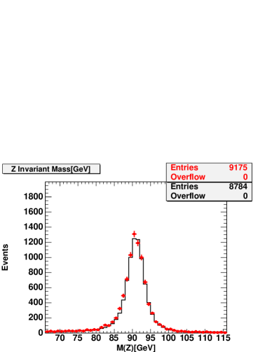
(a) Invariant Mass

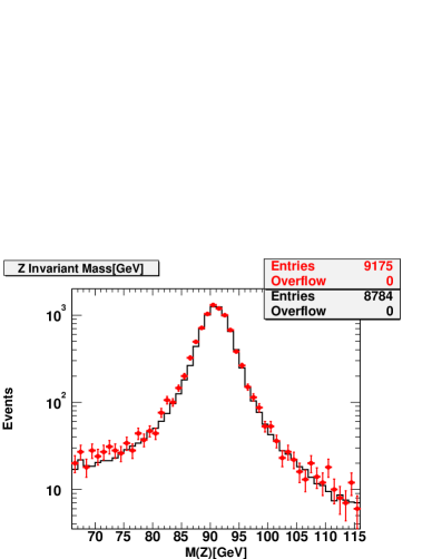
(b) Invariant Mass (log)

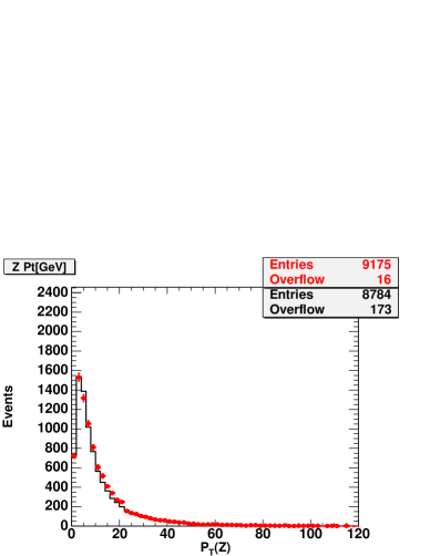
(c) $P_{T}$ of Z${}^{0}\rightarrow\mu^{+}\mu^{-}$

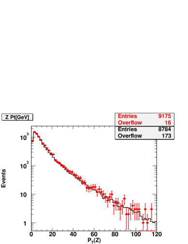
(d) $P_{T}$ of Z${}^{0}\rightarrow\mu^{+}\mu^{-}$ (log)

Figure 5.2: The Z${}^{0}\rightarrow\mu^{+}\mu^{-}$ control sample ‘sanity-check’ plots. The distributions for Invariant Mass of Z${}^{0}\rightarrow\mu^{+}\mu^{-}$, $P_{T}$ of Z${}^{0}\rightarrow\mu^{+}\mu^{-}$, linear plots(a, c), log plots(b, d). The histogram is the prediction from the Z${}^{0}\rightarrow\mu^{+}\mu^{-}$ MC sample; the points are the Z${}^{0}\rightarrow\mu^{+}\mu^{-}$ candidates from the data. Background estimates are not included.

To normalize the Z${}^{0}\rightarrow\mu^{+}\mu^{-}$ MC sample, we used the measured $\sigma$(Z${}^{0}\rightarrow\mu^{+}\mu^{-}$)$\times$BR [62]. The comparison of data vs MC for different muon types is shown in Table 5.7. The Z${}^{0}\rightarrow\mu^{+}\mu^{-}$ event yields are shown in Figure 5.3.

5.2.2 The W${}^{\pm}\rightarrow\mu^{\pm}\nu$ Control Sample

The selection criteria for the W${}^{\pm}\rightarrow\mu^{\pm}\nu$ control sample are listed in Table 5.6. We require one tight muon (${\rm p}_{\rm T}>25$ GeV, see Table 5.2), and $\mbox{${\rm\not\!E}_{\rm T}$}>25$ GeV (Section 8.1). We require the transverse mass of the $W$ candidate to be in the mass window 20-140 GeV.

To reject Z${}^{0}\rightarrow\mu^{+}\mu^{-}$ events in which one muon is not identified, events with a second track with ${\rm p}_{\rm T}>10$ GeV and associated EM and HAD calorimeter energies less than 3 and 9 GeV, respectively, are rejected. We find $118321$ W${}^{\pm}\rightarrow\mu^{\pm}\nu$ events, $59387$ positive and $58934$ negative $W$’s. The W${}^{\pm}\rightarrow\mu^{\pm}\nu$ event yields are shown in Figure 5.3.

Variable	Cut
Tight Muon	Cuts are listed in Table 5.2
Missing $E_{T}$ Cut	$E_{T}>$ 25 GeV
Z-Rejection	No 2nd Track with $P_{T}>10$ GeV, $E_{EM}<3$ GeV, $E_{HAD}<9$ GeV
Mass Window Cut	$M_{T}>20$ GeV and $<140$ GeV
Trigger	MUON_CMUP_18 or MUON_CMX_18

Table 5.6: The selection cuts for the W${}^{\pm}\rightarrow\mu^{\pm}\nu$ control sample.

5.2.3 Summary of the Muon Control Sample Event Counts. Stability Plots

We use the control samples of W${}^{\pm}\rightarrow\mu^{\pm}\nu$ and Z${}^{0}\rightarrow\mu^{+}\mu^{-}$ decays to check temporal stability of the event yields (Figure 5.3). The summary on the number of events in the Muon Sample is shown in Table 5.8.

   

(a) Z${}^{0}\rightarrow\mu^{+}\mu^{-}$

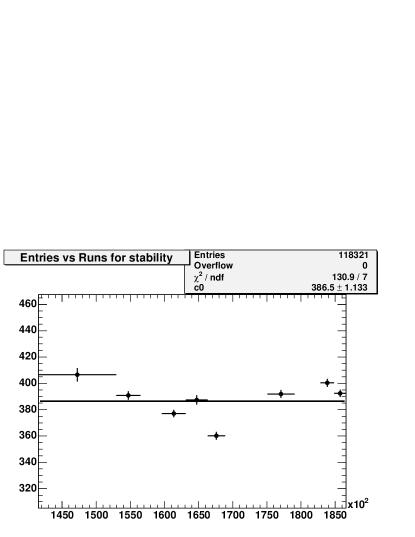
(b) W${}^{\pm}\rightarrow\mu^{\pm}\nu$

Figure 5.3: Stability plots of: (a) the Z${}^{0}\rightarrow\mu^{+}\mu^{-}$, and (b) W${}^{\pm}\rightarrow\mu^{\pm}\nu$ control sample cross sections versus run number. The bins are those of Table 4.1. Shown are the statistical errors, the luminosity systematic error of 6% (Chapter 11) is not included. The trends in Z${}^{0}\rightarrow\mu^{+}\mu^{-}$ (W${}^{\pm}\rightarrow\mu^{\pm}\nu$) are similar to Z${}^{0}\rightarrow e^{+}e^{-}$(W${}^{\pm}\rightarrow e^{\pm}\nu$), see Figure 6.4. We attribute this to common effects (luminosity, trigger, COT).

	DATA	MC
Z${}^{0}\rightarrow\mu^{+}\mu^{-}$
$\mbox{Z${}^{0}\rightarrow\mu^{+}\mu^{-}$}_{ALL~{}Tight}$	3465	3403
$\mbox{Z${}^{0}\rightarrow\mu^{+}\mu^{-}$}_{CMUP-CMUP~{}Tight}$	1462	1428
$\mbox{Z${}^{0}\rightarrow\mu^{+}\mu^{-}$}_{CMUP-CMX~{}Tight}$	1533	1529
$\mbox{Z${}^{0}\rightarrow\mu^{+}\mu^{-}$}_{CMX-CMX~{}Tight}$	470	446
$\mbox{Z${}^{0}\rightarrow\mu^{+}\mu^{-}$}_{ALL}$	9175	8784
$\mbox{Z${}^{0}\rightarrow\mu^{+}\mu^{-}$}_{CMUP-STUBLESS}$	3594	3464
$\mbox{Z${}^{0}\rightarrow\mu^{+}\mu^{-}$}_{CMX-STUBLESS}$	1929	1868

Table 5.7: Z${}^{0}\rightarrow\mu^{+}\mu^{-}$ summary: data vs Z${}^{0}\rightarrow\mu^{+}\mu^{-}$ MC. Background estimates are not included.

Category	N
Events with at least one Tight Muon	180340
Tight Muons	183982
W${}^{\pm}\rightarrow\mu^{\pm}\nu$(triggered+$M_{W}$ window cut)	118321
Tight + Loose Muons	9777
Z${}^{0}\rightarrow\mu^{+}\mu^{-}$(triggered+$M_{Z}$ window cut)	9175

Table 5.8: The numbers of events for the muon control samples. The muon selection cuts are given in Table 5.1, the Z${}^{0}\rightarrow\mu^{+}\mu^{-}$ selection cuts in Table 5.5, and the W${}^{\pm}\rightarrow\mu^{\pm}\nu$ cuts in Table 5.6.

Chapter 6 Electron Identification and Control Samples

We require at least one ‘tight central electron’ in an event for it to be classified as an $e\gamma$ event. In both $e\gamma$ and $\mu\gamma$ events we search for additional ’loose’ electrons in the central and end-plug electromagnetic calorimeters. We describe the tight central and loose central and plug cuts below. The counting experiments based on event counts rather than object counts for the $e\gamma$ candidates are described in Chapter 12. This chapter also describes the control samples of W${}^{\pm}\rightarrow e^{\pm}\nu$ and Z${}^{0}\rightarrow e^{+}e^{-}$ decays used to check the temporal stability, and also the product of acceptance and efficiency.

6.1 Electron Selection Criteria

Variable	Tight	Tight100	Loose
$E_{T}$, $GeV$	$>$ 25	$>$ 100	$>$ 20
Track $P_{T}$, $GeV$	$>$ 10	$>$ 25	$>$ 10
Track $|z0|$, cm	$<$ 60	$<$ 60	$<$ 60
Had/Em	$<$0.055+0.00045$\times$E	$<$0.055+0.00045$\times$E	$<$0.055+0.00045$\times$E
E/P	$<$ 2.0	-	-
Lshr	$<$ 0.2	-	-
Chi2 Strips	$<$ 10	-	-
$\Delta X$, cm	$-3.0<Q_{trk}\times\Delta X<$1.5	$|\Delta X|<$3.0	-
$|\Delta Z|$, cm	$<$ 3.0	$<$ 5.0	-
Fractional Calorimeter Isolation $E_{T}$	$<$ 0.1	$<$ 0.1	$<$ 0.1
Track quality cuts	3$\times$2 SL $\times$5 hits	3$\times$2 SL $\times$5 hits	3$\times$2 SL $\times$5 hits

Table 6.1: Central electron identification and isolation cuts.

The electron selection cuts are similar to the standard CDF Run II cuts [63]. We describe the selection of the tight central electrons in Section 6.1.1. The selection of loose central electrons is described in Section 6.1.2; the selection of electrons in end-plug is presented in Section 6.1.3. The selection cuts are standard [63] with the exception that the CES fiducial requirement (see Section 6.1.1) and the conversion cut (see Sections LABEL:conversions and 10.2) are not applied.

Variable	Tight	Phoenix Tight
$E_{T}$, $GeV$	$>$ 15	$>$ 15
Had/Em	$<$ 0.05	$<$ 0.05
Fractional Calorimeter Isolation $E_{T}$	$<$ 0.1	$<$ 0.1
Chi2 Strips	$<$ 10	$<$ 10
$\Delta R_{xy}$, cm	$<$ 3.0	$<$ 3.0
PES 5by9 U and V	$>$ 0.65	$>$ 0.65
PEM $|\eta|$	2.0 $<|\eta|<$ 1.2	2.0 $<|\eta|<$ 1.2
PhxMatch	-	TRUE
Number of Silicon Hits	-	$\geq$ 3
$|$Z(Phoenix)$|$, cm	-	$<$ 60

Table 6.2: Identification and isolation cuts for the electrons in end-plug. We are using the “Phoenix Tight” selection [64].

6.1.1 Tight Central Electrons

Variable	Cut	Cumulative	This Cut
$e$ Candidates		470379	470379
$E_{T}$, $GeV$	$>$ 25	323506	323506
Track $P_{T}$, $GeV$	$>$ 10; $E_{T}>$ 100 GeV: $>$ 25	316943	324739
Track $|z_{0}|$, cm	$<$ 60	316930	468731
Had/Em	$<$ 0.055 + 0.00045$\times$E	315752	420940
E/P (for $E_{T}<$ 100 GeV only)	$<$ 2.0	308932	365229
Lshr	$<$ 0.2 (for $E_{T}<$ 100 GeV only)	307955	362783
Chi2 Strips	$<$ 10 (for $E_{T}<$ 100 GeV only)	306883	433201
$\Delta X$, cm	-3.0 $<Q_{trk}\times\Delta X<$ 1.5; $E_{T}>$ 100 GeV: $|\Delta X|<$ 3.0	306768	362872
$|\Delta Z|$, cm	$<$ 3.0; $E_{T}>$ 100 GeV: $<$ 5.0	306660	361208
Fractional Calorimeter Isolation $E_{T}$	$<$ 0.1	269624	289848
Track quality cuts	3 Axial, 2 Stereo SL $\times$ 5 hits	269621	398424
Conversion Flag	$\neq$ 1	252900	439187
Fiducial	based on shower max	222844	367024

Table 6.3: Tight central electron identification and isolation cuts. Each entry corresponds to an CDF Central EM object in an event. The column labeled ‘Cumulative’ gives the effect of each successive cut on the number of electron candidates in the $490355$ events in the electron subsample. The heading ‘This Cut’ represents the effect of applying only the cut listed. We do not apply ’Conversion Flag’ and ’Fiducial’ cuts to select electrons, they are tabulated for reference and to see their effects.

The selection criteria for tight central electrons are listed in Table 6.1 and are described below.

Electrons are identified in the CEM by matching high momentum tracks to high-energy CEM clusters. The electron track is the highest momentum track which intersects one of two towers in the CEM cluster. The electron tracks that we use in this analysis are beam-constrained COT-only. We apply the same corrections to the electron tracks as we do to the muon tracks.

Fiduciality is a variable, which can have following values:

• error (null strip/wire cluster)

• not fiducial in central or plug

• fiducial in central or plug

• fiducial, but in CEM Tower 9

• fiducial, but in Chimney wedge tower 7

• fiducial in CEM using max pt track extrapolated to plane of CES

• fiducial in PEM using PES

• fiducial in PEM using max ${\rm p}_{\rm T}$ track extrapolated to plane of PES

An electron candidate is required to have tracking momentum (P) which exceeds half of its calorimeter energy (E). The electron track is required to have a minimum of 3 axial and 2 stereo SL segments containing at least 5 hits each. In order that the momentum resolution does not make for inefficiencies for very high-energy electrons, for $E_{T}>100~{}GeV$ the E/P cut is not applied (leaving only the ${\rm p}_{\rm T}>25$ GeV cut as the requirement on the track). The electrons are required to have the track extrapolate to the beam line within $|z_{0}|<60~{}cm$ so that CDF detector contains the collision well.

The position of the track extrapolated to the CES radius must satisfy the following requirements: it must fall within charge-signed CES shower position of the cluster in the r-phi view -3.0 cm $<Q_{trk}\times\Delta X<$ 1.5 cm and it must fall within 3 cm of the CES shower position in the Z-direction($\Delta Z$).

The CEM shower characteristics should be consistent with that of a single charged particle. We require the ratio of the total energy of the CHA towers located behind the CEM towers in the electron cluster to that of the electron itself to be less than than 0.055+0.00045$\times$E GeV. A comparison of the lateral shower sharing with neighboring towers in the CEM cluster with test-beam data is parameterized by a dimensionless quantity, $L_{shr}$ [39], which must have a value less than 0.2.

     

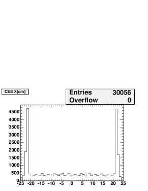
(a) CES X

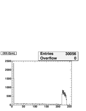
(b) CES Z

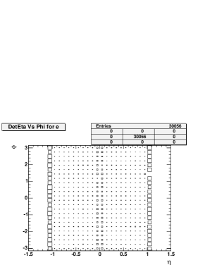
(c) Detector $\eta$ vs. $\phi$

Figure 6.1: Plots for electrons which pass cuts all but CES fiducial requirement.

We require the $\chi^{2}$ for the profile of energy deposited in the CES strips compared to that expected from test beam data [39] to be less than 10. No $\chi^{2}$ cut is made on the profile in the CES wires as bremsstrahlung will separate from the electron in the $r\phi$ view.

As an additional isolation requirement, the total transverse energy deposited in the calorimeter in a cone R=0.4 around the electron track, must be less than 0.1 of the $E_{T}$ of the electron. The isolation is corrected via the standard algorithm [65], for leakage, but not the number of vertices.

We do not apply ’Conversion Flag’ and ’Fiducial’ cuts to select electrons, they are tabulated for reference and to see their effects.

The acceptance gain by removing the fiduciality requirement is approximately 14%. Figure 6.1 shows the distributions for the electrons which pass all cuts but fiducial requirement.

6.1.2 Loose Central Electrons

While each $e\gamma$ event has to contain at least one tight electron, both $e\gamma$ and $\mu\gamma$ events are searched for additional high-${\rm p}_{\rm T}$ electrons that could come from the decays of heavy particles. The cuts for these additional electrons are described in Table 6.1. These cuts are looser than the tight cuts, and in particular do not require any of the CES variables, i.e. no track-cluster match in $\Delta X$ or $\Delta Z$ and no cut on strip $\chi^{2}$, and also no cut on $L_{shr}$ [39].

6.1.3 Plug Electrons

Additional isolated electrons in the plug calorimeter with ${\rm E}_{\rm T}>15$ GeV are identified for measured PEM rapidities of $1.2<|\eta|<2.0$. The cuts used for plug electron identification are given in Table 6.4. We require minimal leakage or activity in the hadron calorimeter, Had/Em $<$ 0.05, a fractional isolation (isolation energy over the electron energy) less than 0.1, and the shower shape to satisfy the PEM 3x3 $\chi^{2}$ and PES 5by9 5-strip to 9 strip ratio cuts. These cuts are similar to standard cuts [63].

We apply face corrections to the PEM energy of the plug electron candidate, add the PPR energy and scale resulting number by 1.0315 [66], as shown in Equation 6.1.

$$\begin{array}[]{l}E_{plug~{}electron}=(E_{pem}^{cor}+E_{ppr})\times 1.0315\end{array}$$ (6.1)

Variable	Cut	Cumulative	This Cut
$e$ Candidates		54247	54247
$E_{T}$	$>$ 15 GeV	15341	15341
Had/Em	$<$ 0.05	11971	37048
Fractional Calorimeter Isolation $E_{T}$	$<$ 0.1	10274	21053
Chi2 Strips	$<$ 10	9931	21708
Delta R	$<$ 3.0 cm	9886	47213
PES 5by9 U and V	$>$ 0.65	9478	25977
PEM $|\eta|$	1.2 $<\eta<$ 2.0	9057	33376
PhxMatch	TRUE	9028	13654
Number of Silicon Hits	$\geq$ 3	8836	11647
$|$Z(Phoenix)$|$	$<$ 60 cm	8836	11733

Table 6.4: Identification and isolation cuts for additional plug electrons.

6.2 Electron Control Samples

As in the muon case, the W and $Z^{0}$ provide control samples for the $e\gamma$ samples. We require at least one tight electron pass the high-${\rm E}_{\rm T}$ electron trigger (ELECTRON_CENTRAL_18) for both W and $Z^{0}$ candidates, where tight electrons are the electrons that pass the cuts in Table 6.1.

For comparisons with data we used the Z${}^{0}\rightarrow e^{+}e^{-}$ MC sample [61]. We applied trigger efficiencies [67] and scale factors [63], which are listed in table 6.5. The CEM Trigger efficiency for high-$E_{T}$ electrons is 1-2.784*exp(-1.749*($E_{T}$ - 17.86)) [67]. The total Track Trigger efficiency is $\approx$ 96-98%, depending on the run number and silicon/non-silicon list of good runs [67].We apply this trigger efficiency to our run-dependent Z${}^{0}\rightarrow e^{+}e^{-}$ MC sample.

Trigger efficiencies
$\epsilon^{trigger}_{CEM}$	1-2.784*exp[-1.749*($E_{T}$ - 17.86)]
$\epsilon^{trigger}_{Track}$	$\approx$0.96-0.98
Scale factors
tight CEM	0.999 $\pm$ 0.006
loose CEM	1.005 $\pm$ 0.005
tight PHX	0.95 $\pm$ 0.01

Table 6.5: Scale factors and trigger efficiencies for the electrons, applied to the Z${}^{0}\rightarrow e^{+}e^{-}$ MC samples.

6.2.1 The $Z^{0}\rightarrow e^{+}e^{-}$ Central-Central Control Sample

The selection criteria for the $Z^{0}\rightarrow e^{+}e^{-}$ central-central control sample are listed in Table 6.6. For this sample a $Z^{0}$ candidate is required to have two central electrons, one passing the tight cuts, and the other the loose cuts (Table 6.1). The mass of the Z candidate is required to be within the window 66 GeV to 116 GeV. The difference in the $z_{0}$ coordinates of the two electron tracks must be less than 4 cm. We find $10128$ opposite-sign events and $199$ same-sign central-central $Z^{0}$ events satisfying these criteria (the large number of same-sign events in the electron sample but not in the muon sample is largely due to photon conversions - see Chapter 10).

Variable	Cut
Tight Electron	Cuts are listed in Table 6.3
Loose Electron	Cuts are listed in Table 6.1
Electron tracks must be of opposite charge	$Q^{e1}+Q^{e2}$ = 0
Delta Z cut	$|Z_{TRACK}^{e1}$ - $Z_{TRACK}^{e2}|<$ 4 cm
Mass Window cut	$M>$ 66 GeV and $<116$ GeV
Trigger	ELECTRON_CENTRAL_18

Table 6.6: The selection cuts for the CC and CP $Z^{0}\rightarrow e^{+}e^{-}$ control samples. The superscripts $e1$ and $e2$ stand for electrons in the event.

The distributions in mass, ${\rm p}_{\rm T}$ of the pair, and $\Delta\phi$ are shown in Figure 6.2. To normalize the Z${}^{0}\rightarrow e^{+}e^{-}$ MC sample, we used the measured $\sigma$(Z${}^{0}\rightarrow\mu^{+}\mu^{-}$)$\times$BR [62].

       

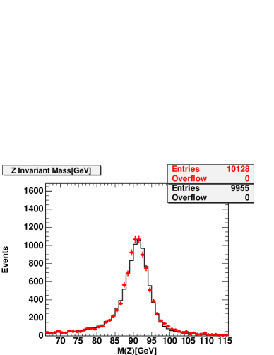
(a) Invariant Mass

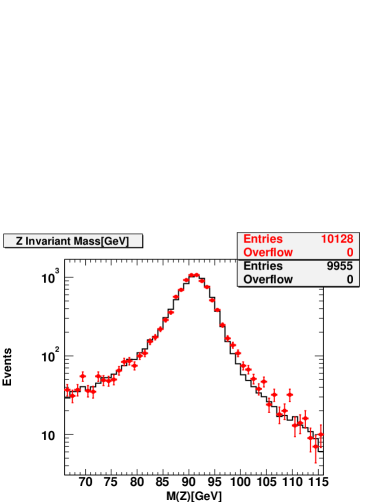
(b) Invariant Mass (log)

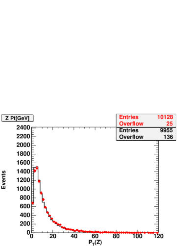
(c) $P_{T}$ of Z${}^{0}\rightarrow e^{+}e^{-}$

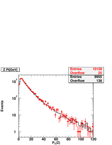
(d) $P_{T}$ of Z${}^{0}\rightarrow e^{+}e^{-}$ (log)

Figure 6.2: The distributions for Invariant Mass of Z${}^{0}\rightarrow e^{+}e^{-}$, $P_{T}$ of Z${}^{0}\rightarrow e^{+}e^{-}$, linear plots(a, c), log plots(b, d). The histogram is the prediction from the Z${}^{0}\rightarrow e^{+}e^{-}$ MC sample (ztop2i), the points are Z${}^{0}\rightarrow e^{+}e^{-}$ candidates in the data. Background estimates are not included.

6.2.2 The $Z^{0}\rightarrow e^{+}e^{-}$ Central-Plug Control Sample

We also form a central-plug dielectron $Z^{0}$ control sample to monitor the identification performance for the electrons in end-plug calorimeters. We require a tight central electron, and a plug electron passing the cuts of Table 6.4. The mass of the Z candidate is required to be within the window 66 GeV to 116 GeV. We find $3996$ ($4004$) central-plug $Z^{0}$ events satisfying these criteria with the plug electron in the East (West) calorimeter.

       

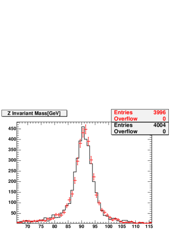
(a) Invariant Mass

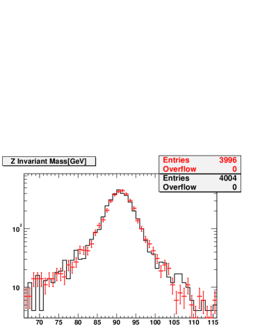
(b) Invariant Mass (log)

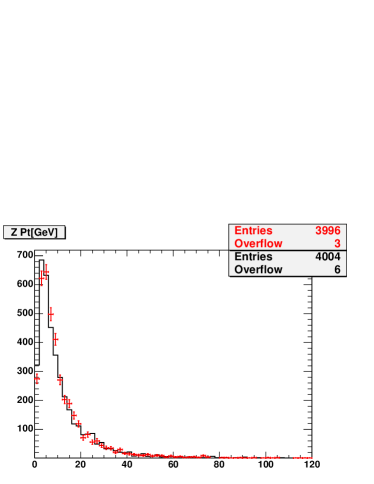
(c) $P_{T}$ of Z${}^{0}\rightarrow e^{+}e^{-}$

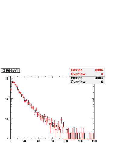
(d) $P_{T}$ of Z${}^{0}\rightarrow e^{+}e^{-}$ (log)

Figure 6.3: Central-plug dielectron Z${}^{0}\rightarrow e^{+}e^{-}$ control sample to monitor the plug electron identification performance. We require a tight central electron(Table 6.3), and a plug electron passing the cuts of Table 6.4. The distributions for Invariant Mass of Z${}^{0}\rightarrow e^{+}e^{-}$, $P_{T}$ of Z${}^{0}\rightarrow e^{+}e^{-}$, linear plots(a, c), log plots(b, d). We find $3996$ ($4004$) central-plug $Z^{0}$ events satisfying these criteria with the plug electron in the East (West) calorimeter. The points are Central-East Plug Z${}^{0}\rightarrow e^{+}e^{-}$ candidates; the histogram is Central-West Plug Z${}^{0}\rightarrow e^{+}e^{-}$ candidates.

The distributions in mass, ${\rm p}_{\rm T}$ of the pair, and $\Delta\phi$ are shown in Figure 6.3. The comparison of data vs MC is shown in Table 6.8. The Z${}^{0}\rightarrow\mu^{+}\mu^{-}$ event yields are shown in Figure 6.4.

6.2.3 The W${}^{\pm}\rightarrow e^{\pm}\nu$ Control Sample

The selection criteria for the W${}^{\pm}\rightarrow e^{\pm}\nu$ control sample are listed in Table 6.7. We require one tight central electron (i.e. $E_{T}>25$ GeV), and corrected ${\rm\not\!E}_{\rm T}$ (Section 8.1) greater than $25$ GeV. We require the transverse mass of the W candidate to be in the mass window 20-140 GeV. We find $184805$ W${}^{\pm}\rightarrow e^{\pm}\nu$ events, $92670$ positive and $92135$ negative W’s. The W${}^{\pm}\rightarrow e^{\pm}\nu$ event yields are shown in Figure 6.4.

Variable	Cut
Tight Electron	Cuts are listed in Table 6.3
Missing $E_{T}$ Cut	$E_{T}>$ 25 GeV
Mass Window Cut	$M_{T}>20$ GeV and $<140$ GeV
Trigger	ELECTRON_CENTRAL_18

Table 6.7: W${}^{\pm}\rightarrow e^{\pm}\nu$ selection cuts.

6.2.4 Summary of the Electron Control Sample Event Counts and Stability Plots

We use the control samples of W${}^{\pm}\rightarrow e^{\pm}\nu$ and Z${}^{0}\rightarrow e^{+}e^{-}$ decays to check temporal stability of the event yields (Figure 6.4). Table 6.8 presents summary of the electron control sample event counts.

       

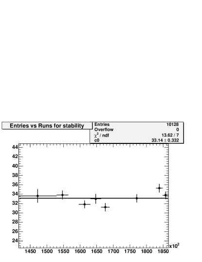
(a) Z${}^{0}\rightarrow e^{+}e^{-}$

(b) W${}^{\pm}\rightarrow e^{\pm}\nu$

(c) Z${}^{0}\rightarrow e^{+}e^{-}$ Central-East

(d) Z${}^{0}\rightarrow e^{+}e^{-}$ Central-West

Figure 6.4: Stability plots for Z${}^{0}\rightarrow e^{+}e^{-}$(a), W${}^{\pm}\rightarrow e^{\pm}\nu$(b), Z${}^{0}\rightarrow e^{+}e^{-}$ Central-East(c), Z${}^{0}\rightarrow e^{+}e^{-}$ Central-West(d). The bins are those of Table 4.1. Shown are the statistical errors, the luminosity systematic error of 6% (Chapter 11) is not included. The trends in Z${}^{0}\rightarrow e^{+}e^{-}$(W${}^{\pm}\rightarrow e^{\pm}\nu$) are similar to Z${}^{0}\rightarrow\mu^{+}\mu^{-}$ (W${}^{\pm}\rightarrow\mu^{\pm}\nu$), see Figure 5.3. We attribute this to some common effects (luminosity, trigger, COT).

	DATA	MC
Z${}^{0}\rightarrow e^{+}e^{-}$
$\mbox{Z${}^{0}\rightarrow e^{+}e^{-}$}_{CC}$	10128	9955
$\mbox{Z${}^{0}\rightarrow e^{+}e^{-}$}_{CCSame-Sign}$	199	127
$\mbox{Z${}^{0}\rightarrow e^{+}e^{-}$}_{CE}$	3996	4257
$\mbox{Z${}^{0}\rightarrow e^{+}e^{-}$}_{CW}$	4004	4131

Table 6.8: Z${}^{0}\rightarrow e^{+}e^{-}$ summary: data vs Z${}^{0}\rightarrow e^{+}e^{-}$ MC. The material is underestimated in MC, so we estimate $e\rightarrow\gamma$ fake rate from data.

Category	N
Events with at least one Tight Electron	254664
Tight Electrons	262555
W${}^{\pm}\rightarrow e^{\pm}\nu$(triggered+$M_{W}$)	184805
Tight + Loose Central Electron	11091
Tight + East Plug Electron	4181
Tight + West Plug Electron	4150
CC Z${}^{0}\rightarrow e^{+}e^{-}$(triggered+$M_{Z}$)	10128
CE Plug Z${}^{0}\rightarrow e^{+}e^{-}$(triggered+$M_{Z}$)	3996
CW Plug Z${}^{0}\rightarrow e^{+}e^{-}$(triggered+$M_{Z}$)	4004

Table 6.9: The numbers of events for the electron control samples. The electron selection cuts are given in Table 6.3, the $Z^{0}\rightarrow e^{+}e^{-}$ selection cuts in Table 6.6, and the W${}^{\pm}\rightarrow e^{\pm}\nu$ selection cuts in Table 6.7. CC refers to Central-Central events; CE refers to Central-East Plug, CW refers to Central-West Plug.

Chapter 7 Photon Identification

The photon selection criteria are identical for photons in both the muon and electron samples; the photon cuts, and the number of events passing in each sample, are enumerated in Table 7.2 and are described below.

A sample of photons from Z${}^{0}\rightarrow e^{+}e^{-}$ events used to measure the probability of an electron radiating an energetic photon is also introduced.

7.1 Photon Selection Criteria

Variable	Cut
$E_{T}^{corr}$	$>$ 25 GeV
Had/Em	$<$ 0.125 or $<$ 0.055 + 0.00045$\times E^{corr}$
$\chi^{2}$ (Strips+Wires)/2.0	$<$ 20
N Tracks	$\leq$ 1
Track $P_{T}$	$<$ 1+0.005$\times E_{T}^{corr}$ GeV
Cone 0.4 Iso$E_{T}^{corr}$	$<$ 2.0+0.02$\times(E_{T}^{corr}-20)$ GeV
Cone 0.4 TrackIso	$<$ 2.0+0.005$\times E_{T}^{corr}$ GeV
2nd CES Cluster (Strip and Wire)	$<$ 2.4+0.01$\times E_{T}^{corr}$ GeV
Fiducial	Ces$|X|<$ 21 cm, 9 cm $<$ Ces $|Z|<$ 230 cm

Table 7.1: Photon identification and isolation cuts.

A photon candidate is required to have corrected transverse energy greater than 25 GeV. For photons or electrons the CES shower position is determined by the energy-weighted centroid of the highest energy clusters of those strips and wires in the CES which correspond to the seed tower. The direction of the photon is determined by the line connecting the primary event vertex to the shower position in the CES. To ensure that events are well-measured the shower position of the photon is required to fall within the fiducial region of the CES so that the shower is fully contained in the active region.

Photon candidates are required to have characteristics consistent with those of a neutral electromagnetically-interacting particle. No COT track with ${\rm p}_{\rm T}>$ 1 GeV may point at the photon cluster. One track with ${\rm p}_{\rm T}<$ 1 GeV may point at the cluster.

The variable ‘Iso$E_{T}^{corr}$’ is the Run I cone $R_{\eta-\varphi}=0.4$ isolation energy with the Run I correction to isolation energy due to phi-crack leakage [65]. The tracking isolation variable ‘Track Isolation’ is the sum of the ${\rm p}_{\rm T}$ of tracks in a in a cone in $\eta-\varphi$ space of radius $R=0.4$ surrounding the photon, measured in GeV.

Table 7.2 summarizes the selection of photons in the muon and electron subsamples (Section 4.1).

Subsample		Muon		Electron
Variable	Cut	Cumulative	This	Cumulative	This
$\gamma$ Candidates		75026	75026	524626	524626
$E_{T}^{corr}$, $GeV$	$>$ 25	4567	4567	333650	333650
HAD/EM	$<$0.125$||\newline$0.055+0.00045$\times E$	4169	68819	330675	499963
$\chi^{2}$ × CES	$<$ 20	2978	39468	279701	389644
N Tracks	$\leq$ 1	2500	58325	210366	371793
Track $P_{T}$, $GeV$	$<$ 1 +0.005$\times E_{T}$	1787	43186	4073	96410
Cone 0.4 Iso$E_{T}^{corr}$, $GeV$	$<$ 2.0+0.02$\times(E_{T}-20)$	1647	19068	3818	302862
Track Isolation, $GeV$	$<$ 2.0+0.005$\times E_{T}$	1610	36352	3771	64776
E (2nd CES Cluster) (Strip and Wire), $GeV$	$<$ 2.4+0.01$\times E_{T}$	1604	67048	3762	471879
Fiducial: Ces$|X|$, Ces$|Z|$, cm	Ces$|X|<$ 21, 9 $<$ Ces$|Z|<$ 230	1598	40879	3735	409371

Table 7.2: Photon identification and isolation cuts. Each entry corresponds to one CDF EM Object, Central or Plug. The column labeled ‘Cumulative’ gives the effect of each successive cut on the number of photon candidates. The heading ‘This’ represents the effect of applying only the one cut listed. After a final cut requiring a Tight muon to be in the event with the photon we find a total of $66$ $\mu\gamma$ candidate events. After a final cut requiring a Tight electron to be in the event with the photon we find a total of $508$ $e\gamma$ candidate events.

For the muon subsample we require the event to be triggered by either a high-${\rm E}_{\rm T}$ muon trigger (which is MUON_CMUP_18 or MUON_CMX_18) or by a high-${\rm E}_{\rm T}$ photon trigger (PHOTON_25_ISO). After requiring a Tight muon (Table 5.1) to be in the event with the photon (Table 7.1) we find a total of $66$ $\mu\gamma$ candidate events.

For the electron subsample we require event to be triggered by either high-${\rm E}_{\rm T}$ electron trigger (ELECTRON_CENTRAL_18) or by high-${\rm E}_{\rm T}$ photon trigger (PHOTON_25_ISO). After requiring a tight electron(Table 6.1) to be in the event with the photon(Table 7.1) we find a total of $508$ $e\gamma$ candidate events. The disparity between this number and the $66$ $\mu\gamma$ events is due to a number of causes, in particular hard photon bremsstrahlung of an electron, as discussed later in Section 7.2.

7.2 Introducing the Photon Control Sample

Unlike for the electron or muon, finding a pure sample of high-Pt photons is difficult; the ‘Compton’ sample of $\gamma$-jet events has QCD fake backgrounds, for example. We describe here a control sample of high-Pt photons derived from the $Z^{0}$.

   

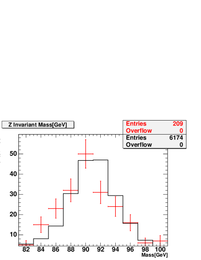
(a) Invariant Mass, GeV

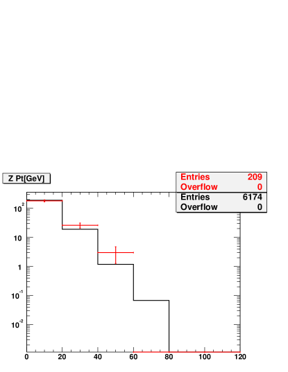
(b) $p_{T}$ of $Z^{0}$, GeV

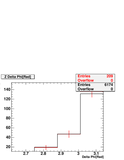
(c) $\Delta\phi$

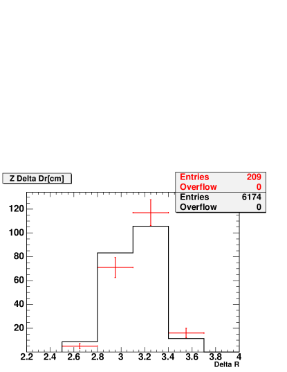
(d) $\Delta R$

Figure 7.1: The distributions for: (a) Invariant Mass of $e+`\gamma`$, (b) $p_{T}$ of $e+`\gamma`$, (c) $\Delta\phi$ of $e+`\gamma`$, (d) $\Delta R$ of $e+`\gamma`$. The points are the $Z^{0}$-like $e\gamma$ sample; the shaded histogram represents electron-electron events from data with the same kinematic cuts, normalized to the number of events in the control sample. Invariant mass for $e+`\gamma`$ is slightly shifted to the left, because energy of the radiated photon is less than energy of the original electron.

In looking for photons in the electron sample, one has to take into account that the dominant source of fake background for $e\gamma$ events is $Z^{0}\rightarrow e^{+}e^{-}$ production, wherein one of the electrons undergoes hard photon bremsstrahlung in the detector material, or the COT fails to detect one of the electron tracks, and that electron subsequently passes all of the photon cuts. There are approximately $7890$ tight central electron pairs in the CDF data, so a photon fake rate as low as $1\%$ will give rise to $158$ $e\gamma$ background events, which would be unacceptably high for finding sources of new physics comparable to $W/Z^{0}+\gamma$ production. The Run II detector has significantly more material inside the outer tracking chamber than the Run I detector had, and so the number of ‘$e\gamma$‘ events from Z${}^{0}\rightarrow e^{+}e^{-}$ production will be significantly higher. We measure this fake rate directly from the data (the material in simulated data is underestimated, see Table 6.8).

A control sample of $Z^{0}$-like events, $e+`\gamma`$, is selected from the $397$ two-body $e\gamma$ candidates (see Chapter 12) by requiring that the invariant mass of the $e\gamma$ pair, $M_{e\gamma}$, be within 10 GeV of the $Z^{0}$ mass (91 GeV). There are $209$ such events in the CDF data. It is observed that the shapes of the distributions of the two samples ($Z^{0}\rightarrow e^{+}e^{-}$ and $e+`\gamma`$) are similar to each other(Figure 7.1).

Chapter 8 Calculating the Missing Transverse Energy and $H_{T}$

This chapter describes how missing transverse energy (${\rm\not\!E}_{\rm T}$) is calculated, and gives the definition and describes calculation of the total transverse energy.

8.1 Calculating the ${\rm\not\!E}_{\rm T}$

Missing transverse energy (${\rm\not\!E}_{\rm T}$) is associated with particles that escape detection. For example, ${\rm\not\!E}_{\rm T}$ is the signature of weakly interacting neutral particles such as neutrinos, or possible new particles such as the gravitino or LSP. It also can come from mismeasurement of the true $E_{T}$ of objects, or from backgrounds such as cosmic rays or beam halo.

Missing $\rm E_{T}$ (${\not\!\!\vec{E}_{T}}$) is defined by ${\not\!\!\vec{E}_{T}}=-\sum_{i}E_{T}^{i}\hat{n}_{i}$, where i is the calorimeter tower number for $|\eta|<$ 3.6, and $\hat{n}_{i}$ is a unit vector perpendicular to the beam axis and pointing at the i^th tower. We define the magnitude $\mbox{${\rm\not\!E}_{\rm T}$}=|{\not\!\!\vec{E}_{T}}|$.

Corrections are made to the ${\rm\not\!E}_{\rm T}$ for non-uniform calorimeter response [56] for jets with uncorrected ${\rm E}_{\rm T}>15$ $GeV$ and $\eta<2.0$, and for muons with ${\rm p}_{\rm T}>20$ $GeV$:

• Muons:
  – correct for $E_{T}-P_{T}$, where $E_{T}$ is a transverse energy deposited in electromagnetic and hadron calorimeters, and $P_{T}$ is a transverse momentum of a muon track. We correct ${\rm\not\!E}_{\rm T}$ for all muons with ${\rm E}_{\rm T}>20$ GeV.

• Jets:
  – correct for $E_{T}-E_{T}^{corr}$, where $E_{T}$ is a transverse energy of an uncorrected jet, and $E_{T}^{corr}$ is a transverse energy of a jet, corrected for non-uniform calorimeter response. We correct for jets with ${\rm E}_{\rm T}^{corr}>15$ GeV.

When identifying jets we check that jet object does not have any of the objects identified in the current analysis close to it (within $\Delta R<$ 0.5).

For the $\ell\gamma\mbox{${\rm\not\!E}_{\rm T}$}$ analysis we set the cut on ${\rm\not\!E}_{\rm T}$ to be $\mbox{${\rm\not\!E}_{\rm T}$}>25$ GeV.

8.2 Calculating the Total Transverse Energy

Total transverse energy ${\rm H}_{\rm T}$ is defined for each event as the sum of the transverse energies of the leptons, photons, jets, and ${\rm\not\!E}_{\rm T}$ that pass the analysis selection criteria. To calculate $H_{T}$ we use Tight and Loose Central Electrons (Table 6.1), Tight Phoenix Electrons (Table 6.2), Tight and Loose CMUP and CMX muons, Stubless muons (Table 5.1), ${\rm\not\!E}_{\rm T}$, and jets in the event with $|\eta|<2$ and $E_{T}^{corr}>15$.

Chapter 9 Standard Model Predictions

The dominant source of $\ell\gamma$ events at the Tevatron is electroweak diboson production (Figure 9.1), in which an electroweak boson ($W$ or $Z^{0}$) decays leptonically ($\ell\nu$ or $\ell\ell$) and a photon is radiated from either an initial state quark, a charged electroweak boson ($W$), or a final state lepton. The number of $\ell\gamma$ events from electroweak diboson production is estimated using several leading-order (LO) Monte Carlo (MC) event generator programs. These programs are MadGraph [68], CompHep [69], and Baur [70, 71].

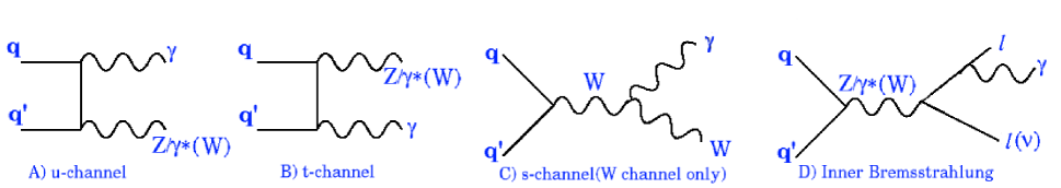
Figure 9.1: Tree-level diagrams for $Z\gamma$ and $W\gamma$ production.

These programs output 4-vectors and helicities of particles emanating from a diboson production event in an ASCII format. In addition the information on how the particles are produced (“mother” and “daughter”) is recorded, including the energy scale and other parameters used for the matrix element calculation.

These files are then fed into the LesHouchesModule [72], which runs Pythia [73] to add parton fragmentation and final-state radiation and initial-state radiation (both QED and QCD) , and then writes out the events in CDF HEPG format. These files are then used as input to the CDF detector simulation program. This program outputs simulated data in a format identical to that of an actual CDF Run II event. Simulated $\ell\gamma$ event rates are then estimated in a manner identical to that of CDF data.

9.1 $W\gamma$, $Z\gamma$, $W\gamma\gamma$ and $Z\gamma\gamma$ MC Sets

The details on the generator level settings of the Baur [71] MC $W\gamma$, $Z\gamma$ datasets can be found in Ref. [74].

The MadGraph $W\gamma$, $Z\gamma$, $W\gamma\gamma$, $Z\gamma\gamma$ datasets created for this analysis are listed in Table 9.3. Details on the MadGraph and CompHep MC samples can be found in Ref. [75, 76].

The kinematic cuts used for the generation of $W\gamma$, $Z\gamma$, $W\gamma\gamma$ and $Z\gamma\gamma$ MC Sets are listed in Table 9.1.

Object	Cuts
MadGraph and CompHep Samples
	${\rm E}_{\rm T}$, $GeV$	$\eta$	$\Delta R$
‘First’ Lepton	6.0	4.0	0.2
Additional Leptons	6.0	4.0	0.2
Neutrinos	1.0	10.0	0
‘First’ Photon	6.0	4.0	0.2
Additional Photons	6.0	4.0	0.2
Baur Samples
	${\rm E}_{\rm T}$, $GeV$	$\eta$	$\Delta R$
‘First’ Lepton	0.0	10.0	0.2
Additional Leptons	0.0	10.0	0.2
Neutrinos	0.0	10.0	0
‘First’ Photon	5.0	10.0	0.2
minimum m($\ell\ell$), $GeV$	$>$20
minimum m($\ell\ell\gamma$), $GeV$	$>$20

Table 9.1: The cuts used at generator level to produce the $Z\gamma$, $W\gamma$, $Z\gamma\gamma$ and $W\gamma\gamma$ samples for CompHep, MadGraph and Baur datasets.

DataSet Name	Events	Cross section (pb)
$Z\gamma$, $W\gamma$
$Z(ee)\gamma$	395482	6.855990
$Z(\mu\mu)\gamma$	395482	6.855990
$Z(\tau\tau)\gamma$	199047	6.423524
$W(e\nu)\gamma$	199831	27.2
$W(\mu\nu)\gamma$ .	199850	27.2
$W(\tau\nu)\gamma$	199891	24.0
$Z\gamma\gamma$, $W\gamma\gamma$
$Z(ee)\gamma\gamma$	198830	0.089137
$Z(\mu\mu)\gamma\gamma$	198830	0.089137
$Z(\tau\tau)\gamma\gamma$	198700	0.078612
$W(e\nu)\gamma\gamma$	199351	0.126
$W(\mu\nu)\gamma\gamma$	199351	0.126
$W(\tau\nu)\gamma\gamma$	198910	0.0939

Table 9.2: The $W\gamma$, $Z\gamma$, $W\gamma\gamma$ and $Z\gamma\gamma$ MadGraph datasets.

DataSet Name	Events	Cross section (pb)
$Z\gamma$, $W\gamma$
$Z(ee)\gamma$	429979	8.62
$Z(\mu\mu)\gamma$	438468	8.61
$W(e\nu)\gamma$	140130	31.9
$W(\mu\nu)\gamma$ .	164732	31.9

Table 9.3: The $W\gamma$ and $Z\gamma$ Baur datasets.

To account for NLO corrections to the $W\gamma$, $Z\gamma$, $W\gamma\gamma$, $Z\gamma\gamma$ processes we use the $E_{T}$-dependent K-factor=${{\sigma_{NLO}}\over{\sigma_{LO}}}$ obtained using Baur’s NLO calculation programs [77].

We apply these corrections to our LO MC(MadGraph and Baur). For $W\gamma\gamma$ and $Z\gamma\gamma$ we used the same K-factor formulas as for $W\gamma$ and $Z\gamma$, respectively.

Since the Baur NLO program only considers the $s$, $t$ and $u$ channel contributions and not the bremstrahlung off the lepton lines(in this case on the generator level $M_{W}\leq 76.0$, $M_{Z}\leq 86.0$) we apply the inclusive W cross-section K-factor of 1.36 to the W+photon processes.

The K-factor applied to $W\gamma$ and $W\gamma\gamma$ MadGraph MC samples is shown in Equation LABEL:kfactor_wgwgg.equation. The K-factor applied to $Z\gamma$ and $Z\gamma\gamma$ MadGraph MC samples is shown in Equation LABEL:kfactor_zgzgg.equation. In the Equations LABEL:kfactor_wgwgg.equation and LABEL:kfactor_zgzgg.equation $M_{W}$($M_{Z}$) is the mass of the generated W(Z) system , and $P_{T}^{\gamma}$ is a (generated) photon transverse energy.

$$\begin{array}[]{l}M_{W}\leq 76.0\Rightarrow K\kern-3.80005pt-\kern-3.80005ptfactor=1.36\\ M_{W}>76.0\Rightarrow K\kern-3.80005pt-\kern-3.80005ptfactor=1.62+0.00001\times P_{T}^{\gamma}-0.386\times exp(-0.100\times P_{T}^{\gamma})\\ \end{array}$$ (9.1)

$$\begin{array}[]{l}M_{Z}\leq 86.0\Rightarrow K\kern-3.80005pt-\kern-3.80005ptfactor=1.36\\ M_{Z}>86.0\Rightarrow K\kern-3.80005pt-\kern-3.80005ptfactor=1.46-0.000728\times P_{T}^{\gamma}-0.125\times exp(-0.0615\times P_{T}^{\gamma})\\ \end{array}$$ (9.2)

Every MC event is weighted with the appropriate K-factor.

9.2 Checks

To be highly confident in the SM predictions, we compared the predictions from the three independent LO matrix-element generators at generator and HEPG level.

There is excellent agreement (within 10% or within statistics) between MadGraph and CompHep in all channels. As the two generators are really different in technique (a helicity amplitude calculation in MadGraph, as opposed to the symbolic evaluation of squared matrix element in CompHep), this gives us confidence in the predictions.

Figure 9.2 shows the integrated cross section versus ${\rm E}_{\rm T}$ of the photon for the MadGraph and CompHep $W\gamma$ and $Z\gamma$ samples [75, 76]. Figure 9.3 shows the integrated cross section versus ${\rm E}_{\rm T}$ of the photon for the MadGraph and CompHep $W\gamma\gamma$ and $Z\gamma\gamma$ samples [75, 76].

   

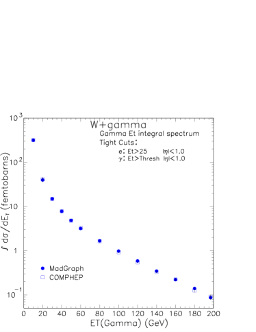
(a) $e\nu\gamma$

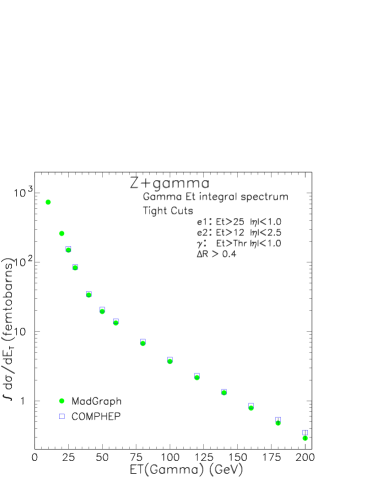
(b) $e^{+}e^{-}\gamma$

Figure 9.2: The integral cross-sections in fb from MadGraph and COMPHEP at 1.96 GeV versus the gamma ${\rm E}_{\rm T}$ for (a) $e\nu\gamma$ production, (b) $e^{+}e^{-}\gamma$ production [75, 76].

   

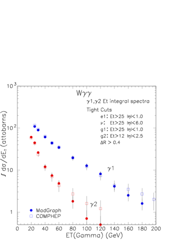
(a) $e\nu\gamma\gamma$

(b) $e^{+}e^{-}\gamma\gamma$

Figure 9.3: The integrated cross section in attobarns ($10^{-3}$ fb or $10^{-6}$ pb) versus the gamma ${\rm E}_{\rm T}$ for for (a) $W\gamma\gamma$ production and (b) $Z\gamma\gamma$ production. The cross section for the highest-${\rm E}_{\rm T}$ photon to be above the threshold is in blue; and the 2nd photon is in red [75, 76].

We have compared MadGraph, CompHep and MadGraph samples at GENERATOR [75] and HEPG [78]. The more detailed study for MadGraph and Baur $Z\gamma$ and $W\gamma$ samples have been performed at Ref. [79, 80]. For example, the distributions for the muon channel is shown in Figure 9.4.

                 

(a) First Lepton $E_{T}$ GeV

(b) Second Lepton $E_{T}$ GeV

(c) Photon $E_{T}$ GeV

(d) First Lepton $\eta$

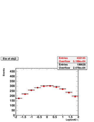
(e) Second Lepton $\eta$

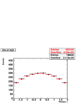
(f) Photon $\eta$

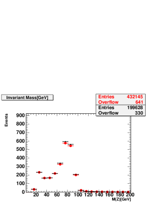
(g) M(Z) GeV

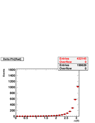
(h) $\Delta\phi(ll)$

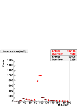
(i) M($Z\gamma$) GeV

Figure 9.4: Comparison of distributions for MadGraph (black) vs Baur(red dots) for $Z\gamma$ ($\mu$ channel) after fragmentation (HEPG level). See [79] for details.

9.3 The SM Diboson $W\gamma$ and $Z\gamma$ Processes as Sources of Lepton-Photon Events

The $W\gamma$ channel was the main SM contributor to the $\ell\gamma\mbox{${\rm\not\!E}_{\rm T}$}$ signature with the Run I cuts [29]. In the Run I analysis, $W\gamma$ was expected to contribute $1.93\pm 0.26$ events to the $e\gamma\mbox{${\rm\not\!E}_{\rm T}$}$ channel, out of a total of $3.41\pm 0.34$, and $1.99\pm 0.27$, out of a total of $4.23\pm 0.46$ for the $\mu\gamma\mbox{${\rm\not\!E}_{\rm T}$}$ channel. Having a reliable prediction of this signature is crucial.

Categories	All Other	1$\ell$, 1$\gamma$, $\Delta\phi_{\ell\gamma}<$150	$\ell\gamma\mbox{${\rm\not\!E}_{\rm T}$}$	Multi-Lepton	Multi-Photon
$W\gamma$, electron channel
MadGraph	15.3$\pm$0.99	1.61$\pm$0.32	13.6$\pm$0.93	0$\pm$0.042	0$\pm$0.042
Baur	15.9$\pm$1.31	2.05$\pm$0.47	13.8$\pm$1.21	0$\pm$0.069	0$\pm$0.069
Average	15.60$\pm$0.82(stat)	1.83$\pm$0.28(stat)	13.70$\pm$0.76(stat)	0.0$\pm$0.040(stat)	0.0$\pm$0.040(stat)
	$\pm$1.70(sys)	$\pm$0.48(sys)	$\pm$1.41(sys)	$\pm$0.0(sys)	$\pm$0.0(sys)
$W\gamma$, muon channel
MadGraph	10.4$\pm$0.77	1.97$\pm$0.34	8.44$\pm$0.70	0$\pm$0.042	0$\pm$0.042
Baur	10.8$\pm$0.95	1.56$\pm$0.36	9.25$\pm$0.88	0$\pm$0.059	0$\pm$0.059
Average	10.60$\pm$0.61(stat)	1.77$\pm$0.25(stat)	8.84$\pm$0.56(stat)	0.0$\pm$0.036(stat)	0.0$\pm$0.036(stat)
	$\pm$1.18(sys)	$\pm$0.45(sys)	$\pm$1.23(sys)	$\pm$0.0(sys)	$\pm$0.0(sys)

Table 9.4: The SM contributions from the $W\gamma$ channel to the analysis categories. The LO calculations from Baur and MadGraph have been corrected by the K-factor and CDF efficiencies. The difference between the two LO generators has been included as a systematic uncertainty (see text); the uncertainty on the average includes both the statistical uncertainties and this systematic uncertainty.

The photon can be radiated from the incoming quarks, from the outgoing electron, or the intermediate W (Figure 9.1). More detail on the kinematic distributions and the cross sections is available in Ref [75]. Initial-state radiation is simulated by the pythia MC program [73] tuned to reproduce the underlying event. The generated particles are then passed through a full detector simulation, and these events are then reconstructed with the same code used for the data.

The predicted numbers of detected $e\gamma$ and $\mu\gamma$ events in $305pb^{-1}$ from SM $W\gamma$ production satisfying the analysis cuts from MadGraph are given in Table 9.4.

The uncertainties on the SM contributions include those from parton distribution functions (5%), factorization scale (2%), K-factor (3%), a comparison of different MC generators ($\sim$ 5%), and the luminosity (6%) (Chapter 11).

We have studied predictions from MadGraph, CompHep and Baur generators for data and MC reconstructed in Ref. [78], and these studies showed good agreement in predicted rates.

The process $\rm p{\bar{p}}\kern-1.79993pt\rightarrow\kern-1.79993ptZ^{0}\kern-2.5pt/\kern-1.49994pt\gamma^{*}+\gamma$ is also one of the major SM backgrounds for the lepton+ photon+X searches. It is the largest contributor to the inclusive multi-body category in the Run I search, with expected contributions in 86 $pb^{-1}$ of 5.01 $\pm$ 0.54 events in the $e\gamma$ mode and 4.60$\pm$0.54 in the $\mu\gamma$ mode [2]. It is also significant in the $\ell\gamma\mbox{${\rm\not\!E}_{\rm T}$}$ channel, especially for muons, as one muon can be missed inducing ${\rm\not\!E}_{\rm T}$. The expected contributions for the electron and muon channels in Run I were $0.32\pm 0.5$ and $0.96\pm 0.15$ events, respectively, smaller than the $W\gamma$ contributions, but still significant, with a total ($e+\mu$) of $1.27\pm 0.17$ events out of the $7.64\pm 0.71$ events expected in 86 $pb^{-1}$.

The photon can be radiated from the incoming quarks or from the outgoing electron (Figure 9.1). More detail on the kinematic distributions and the cross sections is available in Ref [75].

The predicted numbers of detected (inclusive) $e\gamma$ and $\mu\gamma$ events in $305pb^{-1}$ from SM $Z\gamma$ production satisfying the analysis cuts from MadGraph are given in Table 9.5. The uncertainties on the SM contributions include those from parton distribution functions (7%), a comparison of different MC generators ($\sim$ 5%), and the luminosity (6%) (Chapter 11).

Categories	All Other	1$\ell$, 1$\gamma$, $\Delta\phi_{\ell\gamma}<$150	$\ell\gamma\mbox{${\rm\not\!E}_{\rm T}$}$	Multi-Lepton	Multi-Photon
$Z\gamma$, electron channel
MadGraph	21$\pm$0.39	7.77$\pm$0.24	0.97$\pm$0.084	12.1$\pm$0.29	0.12$\pm$0.030
Baur	22.7$\pm$0.43	8.31$\pm$0.26	1.34$\pm$0.11	12.9$\pm$0.33	0.17$\pm$0.038
Average	21.85$\pm$0.29(stat)	8.04$\pm$0.18(stat)	1.16$\pm$0.069(stat)	12.50$\pm$0.22(stat)	0.15$\pm$0.024(stat)
	$\pm$2.80(sys)	$\pm$0.98(sys)	$\pm$0.39(sys)	$\pm$1.51(sys)	$\pm$0.052(sys)
$Z\gamma$, muon channel
MadGraph	15.7$\pm$0.32	3.46$\pm$0.15	4.28$\pm$0.17	7.96$\pm$0.22	0.026$\pm$0.013
Baur	16.6$\pm$0.35	4.18$\pm$0.18	4.7$\pm$0.19	7.67$\pm$0.23	0.022$\pm$0.013
Average	16.15$\pm$0.24(stat)	3.82$\pm$0.12(stat)	4.49$\pm$0.13(stat)	7.81$\pm$0.16(stat)	0.024$\pm$0.01(stat)
	$\pm$1.92(sys)	$\pm$0.82(sys)	$\pm$0.63(sys)	$\pm$0.87(sys)	$\pm$0.0047(sys)

Table 9.5: The SM contributions from the $Z\gamma$ electron channel to the analysis categories. The LO calculations from Baur and MadGraph have been corrected by the K-factor and CDF efficiencies. The difference between the two LO generators has been included as a systematic uncertainty (see text); the uncertainty on the average includes both the statistical uncertainties and this systematic uncertainty.

9.4 The SM Triboson $W\gamma\gamma$ and $Z\gamma\gamma$ Processes as Sources of Lepton-Photon Events

While small, the $W\gamma\gamma$, $Z\gamma\gamma$ processes are the largest true SM sources of a signature of a high-${\rm p}_{\rm T}$ lepton plus two photons. The observation of several such events has motivated a careful study of the cross-sections for these sources [75]. In this study we have used both MadGraph and Comphep; we get excellent agreement between the two generators (Figure 9.3), giving us confidence in the predictions.

The final state of one lepton and two photons, $\ell\nu\gamma\gamma$, is produced in the SM through an intermediate W, with radiation off of any of the charged lines in the diagrams. We denote the final state of $\ell\nu\gamma\gamma$ as ‘$W\gamma\gamma$’ for convenience, although the $W$ is virtual and the kinematics of the final state are more complicated than the name would suggest. Note that this is process has three spin-one bosons in the final state; MadGraph treats the helicities correctly and writes them into the output file as input to the next steps.

The predicted numbers of detected $e\gamma$ and $\mu\gamma$ events in $305pb^{-1}$ from SM $W\gamma\gamma$ production satisfying the analysis cuts from MadGraph are given in Table 9.6. The agreement on the generator level for $W\gamma\gamma$ between the two monte carlos, CompHep and MadGraph is good (Figure 9.3), and we will use MadGraph $W\gamma\gamma$ to get predicted rates. More details, including kinematic distributions, can be found in Ref. [75].

Categories	All Other	1$\ell$, 1$\gamma$, $\Delta\phi_{\ell\gamma}<$150	$\ell\gamma\mbox{${\rm\not\!E}_{\rm T}$}$	Multi-Lepton	Multi-Photon
$W\gamma\gamma$, electron channel
MadGraph	0.14$\pm$	0.019$\pm$	0.11$\pm$	0.0052$\pm$	0.0067$\pm$
	0.0064(stat)	0.0023(stat)	0.0057(stat)	0.0012(stat)	0.0014(stat)
	$\pm$0.017(sys)	$\pm$0.0023(sys)	$\pm$0.013(sys)	$\pm$6.2e-04(sys)	$\pm$8.0e-04(sys)
$W\gamma\gamma$, muon channel
MadGraph	0.069$\pm$	0.0100$\pm$	0.055$\pm$	0.0$\pm$	0.0037$\pm$
	0.0042(stat)	0.0016(stat)	0.0037(stat)	1.9e-04(stat)	9.5e-04(stat)
	$\pm$0.0083(sys)	$\pm$0.0012(sys)	$\pm$0.0066(sys)	$\pm$0.0(sys)	$\pm$4.4e-04(sys)
$Z\gamma\gamma$, electron channel
MadGraph	0.54$\pm$	0.26$\pm$	0.029$\pm$	0.24$\pm$	0.015$\pm$
	0.0100(stat)	0.0070(stat)	0.0023(stat)	0.0067(stat)	0.0017(stat)
	$\pm$0.065(sys)	$\pm$0.031(sys)	$\pm$0.0035(sys)	$\pm$0.029(sys)	$\pm$0.0018(sys)
$Z\gamma\gamma$, muon channel
MadGraph	0.37$\pm$	0.12$\pm$	0.12$\pm$	0.12$\pm$	0.011$\pm$
	0.0080(stat)	0.0046(stat)	0.0046(stat)	0.0044(stat)	0.0014(stat)
	$\pm$0.044(sys)	$\pm$0.014(sys)	$\pm$0.014(sys)	$\pm$0.014(sys)	$\pm$0.0013(sys)

Table 9.6: The predicted number of $\ell\gamma+X$ events in $305pb^{-1}$ from SM $W\gamma\gamma$ and $Z\gamma\gamma$ production satisfying the analysis cuts from MadGraph. The uncertainty includes both the statistical uncertainties and this systematic uncertainty.

The final state of two leptons and two photons, $\ell\ell\gamma\gamma$, is generated through the intermediate photon and $Z^{0}$ states, with radiation off of any of the charged lines in the diagrams. We denote this as ‘$Z\gamma\gamma$’ for convenience, but the two amplitudes modify the mass spectra and angular distributions, and so are both important.

This process is one of the SM mechanisms that could produce the $\mu\mu\gamma\gamma jj$ event [28] (although with an extra two jets), and is of interest in the dilepton-diphoton searches as a background. As one can see below the SM cross sections are small, typically one femtobarn or less.

The predicted numbers of detected $e\gamma$ and $\mu\gamma$ events in $305pb^{-1}$ from SM $Z\gamma\gamma$ production satisfying the analysis cuts from MadGraph are given in Table 9.6. The agreement on the generator level for $W\gamma\gamma$ between the two monte carlos, CompHep and MadGraph is good (Figure 9.3), and we will use MadGraph $W\gamma\gamma$ to get predicted rates. More details, including kinematic distributions, can be found in Ref. [75].

9.5 The Sum of Contributions for SM $W\gamma$, $Z\gamma$, $W\gamma\gamma$, $Z\gamma\gamma$ Processes

Table 9.7 gives the sum of the expected contributions to the $e\gamma$ and $\mu\gamma$ channels from SM $W\gamma$, $Z\gamma$, $W\gamma\gamma$, and $Z\gamma\gamma$ processes. We have multiplied the average LO predictions for each channel by the K-factors listed in Equations LABEL:kfactor_wgwgg.equation and LABEL:kfactor_zgzgg.equation. As we require the event to be triggered either by the lepton or by the photon trigger, this combination of triggers is fully efficient.

Categories	All Other	1$\ell$, 1$\gamma$, $\Delta\phi_{\ell\gamma}<$150	$\ell\gamma\mbox{${\rm\not\!E}_{\rm T}$}$	Multi-Lepton	Multi-Photon
$e\gamma$	38.13$\pm$0.87(stat)	10.15$\pm$0.33(stat)	15.00$\pm$0.76(stat)	12.75$\pm$0.22(stat)	0.17$\pm$0.047(stat)
	$\pm$4.58(sys)	$\pm$1.49(sys)	$\pm$1.82(sys)	$\pm$1.54(sys)	$\pm$0.055(sys)
$\mu\gamma$	27.19$\pm$0.66(stat)	5.72$\pm$0.28(stat)	13.51$\pm$0.57(stat)	7.93$\pm$0.16(stat)	0.039$\pm$0.037(stat)
	$\pm$3.15(sys)	$\pm$1.29(sys)	$\pm$1.88(sys)	$\pm$0.88(sys)	$\pm$0.0064(sys)
$\ell\gamma$	65.32$\pm$1.09(stat)	15.87$\pm$0.44(stat)	28.51$\pm$0.95(stat)	20.68$\pm$0.28(stat)	0.21$\pm$0.060(stat)
	$\pm$7.74(sys)	$\pm$2.78(sys)	$\pm$3.70(sys)	$\pm$2.42(sys)	$\pm$0.061(sys)

Table 9.7: The sum of the expected contributions to the $e\gamma$ and $\mu\gamma$ channels from SM $W\gamma$, $Z\gamma$, $W\gamma\gamma$, and $Z\gamma\gamma$ processes. The average of the two LO predictions for each channel has been multiplied by the K-factors listed in Equations LABEL:kfactor_wgwgg.equation and  LABEL:kfactor_zgzgg.equation.

9.6 $W\gamma$ and $Z\gamma$ Followed by W${}^{\pm}\rightarrow\tau^{\pm}\nu$ or $Z\kern-1.79993pt\rightarrow\kern-1.79993pt{\tau^{+}\tau^{-}}$ and $\tau\rightarrow e\nu\nu$ or $\mu\nu\nu$

The last SM direct contribution (as opposed to misidentification) we consider is $W\gamma$ and $Z\gamma$ production followed by the boson leptonic decay in the $\tau$ channel(“$\tau\gamma$ background”). The tau can then decay into an electron or muon. These events are not fakes, in the sense that the electron or muon is real, although not a direct product of the vector boson decay.

Table 9.8 gives a summary of the contributions to the $e\gamma$ and $\mu\gamma$ channels from $\tau\gamma$ events ($W\gamma$ and $Z\gamma$ decaying to taus). Shown are numbers of expected tau events from different processes ($W\gamma$, $Z\gamma$) making a signature of $e\gamma$, $\mu\gamma$ and $l\gamma$ for the different categories defined in the analysis. The final lepton is either an electron or muon.

Categories	All Other	1$\ell$, 1$\gamma$, $\Delta\phi_{\ell\gamma}<$150	$\ell\gamma\mbox{${\rm\not\!E}_{\rm T}$}$	Multi-Lepton	Multi-Photon
$e\gamma$	1.13$\pm$0.20(stat)	0.42$\pm$0.12(stat)	0.71$\pm$0.16(stat)	0$\pm$0.041(stat)	0$\pm$0.041(stat)
	$\pm$0.14(sys)	$\pm$0.051(sys)	$\pm$0.085(sys)	$\pm$0(sys)	$\pm$0(sys)
$\mu\gamma$	0.66$\pm$0.12(stat)	0.38$\pm$0.11(stat)	0.26$\pm$0.072(stat)	0.013$\pm$0.042(stat)	0$\pm$0.041(stat)
	$\pm$0.079(sys)	$\pm$0.045(sys)	$\pm$0.031(sys)	$\pm$0.0016(sys)	$\pm$0(sys)
$\ell\gamma$	1.79$\pm$0.24(stat)	0.80$\pm$0.16(stat)	0.97$\pm$0.18(stat)	0.013$\pm$0.059(stat)	0$\pm$0.059(stat)
	$\pm$0.21(sys)	$\pm$0.096(sys)	$\pm$0.12(sys)	$\pm$0.0016(sys)	$\pm$0(sys)

Table 9.8: SM contributions from $\tau\gamma$ events ($W\gamma$ and $Z\gamma$ decaying to taus).

Background from $W\kern-1.79993pt\rightarrow\kern-1.79993pt\tau\nu$, where $\tau\kern-1.79993pt\rightarrow\kern-1.79993pt\rho\nu$ ($\approx$1/4 of the $\tau$ branching fraction), then $\rho\kern-1.79993pt\rightarrow\kern-1.79993pt\pi\pi^{0}$, which could mimic a single track + photon signature that looks like $\ell\gamma\mbox{${\rm\not\!E}_{\rm T}$}$ is a part of $\tau\gamma$ background estimated.

Chapter 10 Backgrounds: Fakes

In addition to the expectations from real SM processes that produce real $\ell\gamma$ events described in Chapter 9, there are backgrounds due to misidentified leptons and photons, and also incorrectly calculated ${\rm\not\!E}_{\rm T}$. We generically call these misidentifications ‘fakes’. In this chapter we first treat backgrounds from fake photons, then from fake leptons, including backgrounds to the W samples due to events with a fake lepton and false ${\rm\not\!E}_{\rm T}$.

10.1 Fake Photons

We consider two sources of fake photons: QCD jets in which a neutral hadron or photon from hadron decay mimics a direct photon, and electron bremsstrahlung, in which an energetic photon is radiated off of an electron which is then much lower energy and curls away from the photon.

10.1.1 Fake Photons from Jets

High ${\rm p}_{\rm T}$ photons are copiously created from hadron decays in jets initiated by a scattered quark or gluon. In particular, mesons such as the $\pi^{0}$ or $\eta$ decay to photons which may satisfy the photon selection criteria.

The number of lepton-plus-misidentified-jet events in the $\ell\gamma\mbox{${\rm\not\!E}_{\rm T}$}$ and $\ell\ell\gamma$ samples is determined by measuring the jet ${\rm E}_{\rm T}$ spectrum in $\ell\mbox{${\rm\not\!E}_{\rm T}$}+$jet and $\ell\ell+$jet samples, respectively, and then multiplying by the probability of a jet being misidentified as a photon, $P^{jet}_{\gamma}({\rm E}_{\rm T})$. The uncertainty on the number of such events is calculated by again using the measured jet spectrum and the upper and lower bounds on the ${\rm E}_{\rm T}$-dependent misidentification rate. An overview of the fake rate method is given in Ref. [41].

   

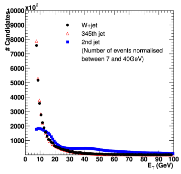
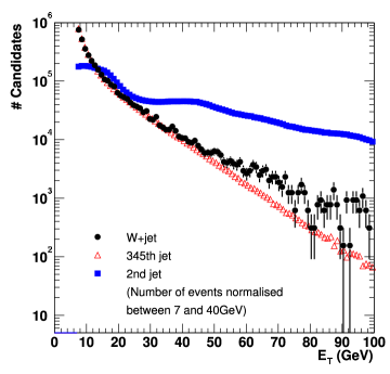
Figure 10.1: The dN/d${\rm E}_{\rm T}^{jet}$ vs ${\rm E}_{\rm T}^{jet}$ distribution for jets in W sample (black points) and in jet samples. 2nd high-${\rm E}_{\rm T}$jet in the jet samples is shown in blue squares and the 345th jet in red open triangles.

Any photon that is due the decay of a meson ($\pi^{0}\rightarrow\gamma\gamma$, $\eta\rightarrow\gamma\gamma$) is classified as FAKE and any photon that is created in the hard scattering process or radiated off a quark is classified as a TRUE photon. The strategy is first to measure the RAW fake rate. The fraction of jets which are matched to a photon candidate

$$P_{RAW}({\rm E}_{\rm T}^{jet})=\frac{N_{\gamma-candidate}}{N_{jet}}=\frac{N_{\gamma}^{TRUE}+N_{\gamma}^{FAKE}}{N_{jet}}$$ (10.1)

We estimate TRUE fake as

$$P_{TRUE}({\rm E}_{\rm T}^{jet})=P_{RAW}({\rm E}_{\rm T}^{jet})\times F_{QCD},~{}~{}F_{QCD}=\frac{N_{\gamma}^{FAKE}}{N_{\gamma}^{TRUE}+N_{\gamma}^{FAKE}}$$ (10.2)

To distinguish $\gamma$ from $\pi^{0}$ or other hadrons, the following variables have been used in the jet fake rate studies:

• CES $\chi^{2}$
  – $\pi^{0}\rightarrow\gamma\gamma$ typically have higher $\chi^{2}$ than prompt photons

• Isolation in a cone in $\eta-\varphi$ space of radius R=0.4 around the $\gamma$ candidate
  – the background is usually produced as a part of a jet $\Rightarrow$ ${\rm E}_{\rm T}$ is higher than for $\gamma$

• Hit rate in the CPR (Central Preradiator Detector, see Section 2.2.3)
  – CPR is between solenoid and calorimeter. $\gamma$ converts in the coil and therefore we measure charge. Photons and fakes have different conversion probabilities.

   

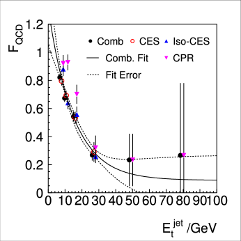
(a) $F_{QCD}$

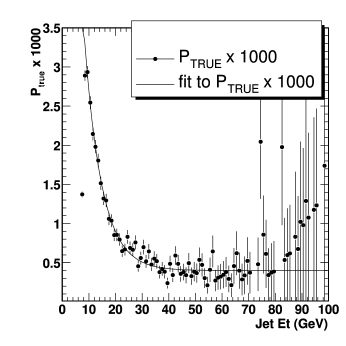
(b) $P_{TRUE}^{jet\rightarrow\gamma}$

Figure 10.2: (a) $F_{QCD}$; (b) a probability for a jet to fake a photon.

Technical details on the studies of jets faking photons in CDF II are available in Ref. [81]. The most recent numbers are available in Ref. [41] and resulting distribution for $F_{QCD}$ and $P_{TRUE}$ are shown in Figure 10.2. We follow this study closely in our estimates. We use jets from the inclusive high-${\rm p}_{\rm T}$ muon and high-${\rm E}_{\rm T}$ electron lepton samples (Section 4.1) to evaluate the background from jets faking photons.

The above studies show that the (fake) photon carries about 94% of the jet $E_{T}$, and the resolution on the photon $E_{T}$ is about 5%. We consequently scale and smear the jet $E_{T}$ by these numbers to get the $E_{T}$ of the fake photon. We then select jets with $|\eta|<1.1$ and $E_{T}>$ 25 GeV after the scaling and smearing. The jets are then weighted with by the jet fake rate [81].

       

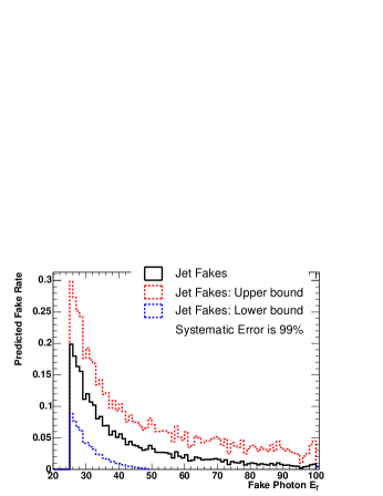
(a) $\ell\gamma\mbox{${\rm\not\!E}_{\rm T}$}$ (Electron Channel)

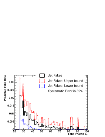
(b) $\ell\ell\gamma$ (Electron Channel)

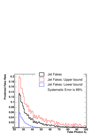
(c) $\ell\gamma\mbox{${\rm\not\!E}_{\rm T}$}$ (Muon Channel)

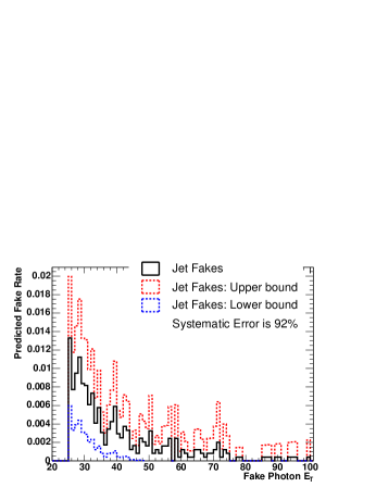
(d) $\ell\ell\gamma$ (Muon Channel)

Figure 10.3: The $E_{T}$ spectrum of events expected in $305pb^{-1}$ with a fake photon from a jet versus the $E_{T}$ of the fake photon. The four plots show the number of events per 2 GeV bin expected in the $\ell\gamma\mbox{${\rm\not\!E}_{\rm T}$}$ and $\ell\ell\gamma$ signatures in both the electron and muon channels. The upper and lower error bands from Ref. [41] are shown.

Categories	All Other	1 $l$, 1 $\gamma$, $\Delta\phi<$150	$\ell\gamma\mbox{${\rm\not\!E}_{\rm T}$}$	Multi-Lepton	Multi-Photon
$e\gamma$	$3.76$$\pm$$3.76$(tot)	$0.69$ $\pm$$0.69$(tot)	$2.8$ $\pm$$2.8$(tot)	$0.3$ $\pm$$0.3$(tot)	$0.0003$ $\pm$$0.0003$(tot)
$\mu\gamma$	$1.88$$\pm$$1.88$(tot)	$0.14$ $\pm$$0.14$(tot)	$1.6$ $\pm$$1.6$(tot)	$0.2$ $\pm$$0.2$(tot)	$0.00008$ $\pm$$0.00008$(tot)
$\ell\gamma$	$5.64$$\pm$$5.64$(tot)	$0.83$ $\pm$$0.83$(tot)	$4.40$ $\pm$$4.40$(tot)	$0.50$ $\pm$$0.50$(tot)	$0.00038$ $\pm$$0.00038$(tot)

Table 10.1: The predicted backgrounds from jets faking photons in the analysis subcategories. We estimate systematic uncertainty on the predicted number to be 100%. Statistical errors are negligible. The uncertainties in the electron and muon samples are assumed to be 100% correlated.

The number of fake events versus the $E_{T}$ of the fake photon are shown in Figure 10.3 for the $\ell\gamma\mbox{${\rm\not\!E}_{\rm T}$}$ and $\ell\ell\gamma$ samples in both the electron and muon channels. We count lepton-‘fake photon‘ candidates in the same way as we do for real photons to calculate background for each subcategory. Table 10.1 summarizes the number of events in the $e\gamma$ and $\mu\gamma$ samples for the sub-categories used in the analysis.

10.1.2 Fake Photons from Electron Bremsstrahlung

We can measure the probability that a high-${\rm E}_{\rm T}$ electron ‘brems’ an energetic photon in the material before the COT tracking volume in such a way that it fakes a photon, by using the $Z^{0}$ as a source of ‘tagged’ electrons. We look for a back-to-back $e^{+}e^{-}$ pair close to the $Z^{0}$ mass ($\Delta\phi_{ee}>150^{\circ}$ and $81~{}GeV<M_{ee}<101~{}GeV$) - this is the sub-category labeled ‘Z-like’. For the $e\gamma$ sample the requirements are an exactly 1 electron and 1 photon, with $\Delta\phi_{e\gamma}>150^{\circ}$ and $81~{}GeV<m_{e\gamma}<101~{}GeV$. From the number of these events and the number of Z${}^{0}\rightarrow e^{+}e^{-}$ events we can measure the probability per ‘leg’ of a $Z^{0}$ that an electron is misidentified as a photon. We require both electrons in Z${}^{0}\rightarrow e^{+}e^{-}$ to be central and pass tight cuts, so that the kinematic requirements will be the same as for the $e\gamma$ sample (i.e. two tight central electromagnetic objects).

The events in the 2nd row (labeled as Z${}^{0}\rightarrow e^{+}e^{-}$) of the Table 10.2 have the same signature as $\ell\gamma$ events (see Figure 12.1), but instead of a photon we require a tight central electron(Table 6.3).

For instance, to estimate contribution from electron faking photon to $\ell\gamma\mbox{${\rm\not\!E}_{\rm T}$}$ category we count events with ee+${\rm\not\!E}_{\rm T}$ (both electrons are tight central, Table 6.3). For Multi-Lepton + Photon we count events with three electrons, of which two electrons should be tight central, and the third one can be tight or loose central (Table 6.1), or phoenix tight (Table 6.2). Finally, for Multi-Photon + Lepton category we use $ee\gamma$ events, both electrons are Tight Central.

Using the numbers in Table 10.2 we calculate the background from electrons misidentified as photons. For example, for $e\gamma\mbox{${\rm\not\!E}_{\rm T}$}$ subcategory the estimated number of electron-fake-photon events(“$e~{}\rightarrow~{}\gamma~{}fakes$”) is calculated as follows:

$$N^{e~{}\rightarrow~{}\gamma~{}fakes}_{e\gamma\mbox{${\rm\not\!E}_{\rm T}$}}=N^{\mbox{Z${}^{0}\rightarrow e^{+}e^{-}$}}_{ee\mbox{${\rm\not\!E}_{\rm T}$}}\times\frac{N^{e\gamma}_{Z^{0}-like}-N^{diboson}_{Z^{0}-like}-N^{jets}_{Z^{0}-like}}{N^{\mbox{Z${}^{0}\rightarrow e^{+}e^{-}$}}_{Z^{0}-like}}$$ (10.3)

• $N^{\mbox{Z${}^{0}\rightarrow e^{+}e^{-}$}}_{ee\mbox{${\rm\not\!E}_{\rm T}$}}~{}\equiv$ $ee\mbox{${\rm\not\!E}_{\rm T}$}$ events in the Z${}^{0}\rightarrow e^{+}e^{-}$ sample

• $N^{e\gamma}_{Z^{0}-like}~{}~{}~{}~{}~{}~{}~{}~{}\equiv$ $e\gamma$ $Z^{0}$-like events

• $N^{diboson}_{Z^{0}-like}~{}~{}~{}~{}~{}~{}~{}~{}\equiv$ $e\gamma$ $Z^{0}$-like events expected from diboson events($W\gamma$, $Z\gamma$)

• $N^{jets}_{Z^{0}-like}~{}~{}~{}~{}~{}~{}~{}~{}\equiv$ $e$+jet faking photon $Z^{0}$-like events expected from misidentified jets

• $N^{\mbox{Z${}^{0}\rightarrow e^{+}e^{-}$}}_{Z^{0}-like}~{}\equiv$ Z${}^{0}\rightarrow e^{+}e^{-}$ events (81 GeV $<M_{Z}^{0}<$ 101 GeV, $\Delta\phi_{ee}>$ 150)

We take all numbers from data, with the exception that we get number of $Z^{0}-like$ events expected from diboson events, $W\gamma$ and $Z\gamma$, from MC (we take into account contribution from $Z\gamma\gamma$ and $W\gamma\gamma$, although it’s $\approx$ 1% of that from $Z\gamma$ and $W\gamma$).

Finally, we estimate the number of electron-fake-photon events in $\ell\gamma\mbox{${\rm\not\!E}_{\rm T}$}$ to be

$$N^{e~{}\rightarrow~{}\gamma~{}fakes}_{e\gamma\mbox{${\rm\not\!E}_{\rm T}$}}=76*\frac{209\pm 14.45-9.03\pm 0.23-0.97\pm 0.97}{6174}=2.45\pm 0.33$$ (10.4)

Categories	$Z^{0}$-like	All Other	1 $l$, 1 $\gamma$, $\Delta\phi<$150	$\ell\gamma\mbox{${\rm\not\!E}_{\rm T}$}$	Multi-Lepton	Multi-Photon
Z${}^{0}\rightarrow e^{+}e^{-}$	$6174$	$723$	$637$	$76$	$7$	$6$
Diboson	$9.03\pm 0.23$	$38.13\pm 0.87$	$10.15\pm 0.33$	$15.00\pm 0.76$	$12.75\pm 0.22$	$0.17\pm 0.047$
Jet fakes	$0.97\pm 0.97$	$3.76\pm 3.76$	$0.69\pm 0.69$	$2.8\pm 2.8$	$0.3\pm 0.3$	$0.0003\pm 0.0003$
$e\kern-1.61993pt\rightarrow\kern-1.61993pt\gamma$ fakes	$199.00\pm 14.67$	$23.30\pm 1.90$	$20.53\pm 1.70$	$2.45\pm 0.33$	$0.23\pm 0.09$	$0.193\pm 0.080$

Table 10.2: Bottom row: The calculated number of events in each analysis subcategory for electrons faking photons by catastrophic bremsstrahlung. The upper three rows are the input numbers used in the calculation, which is given by Equation 10.3. Only statistical errors are quoted. Systematic errors estimated by varying Z mass window are found to be negligible.

Table 10.2 summarizes the calculated number of events in each analysis subcategory for electrons faking photons by catastrophic bremsstrahlung. The upper three rows are the input numbers used in the calculation, which is given by Equation 10.3. The last row gives the estimated number of events detected with fake photons from electron bremsstrahlung.

10.2 QCD (’Non-W/Z’) Backgrounds

To measure the QCD backgrounds from fake leptons and or fake ${\rm\not\!E}_{\rm T}$, we form a ‘non-W/Z’ sample we expect to have very little real lepton content [82] by selecting on loose leptons, rejecting events from the W or Z.

To estimate Non-W/Z background we use four samples:

• Non-W/Z sample: 1 $\ell$ + jet(s), no W or Z candidates

• Signal Sample: $\ell\gamma\mbox{${\rm\not\!E}_{\rm T}$}$ or $ll\gamma$

• Golden-Lepton: tight e’s, CC Z${}^{0}\rightarrow e^{+}e^{-}$; tight $\mu$’s Z${}^{0}\rightarrow\mu^{+}\mu^{-}$

• Jet Faking Photon: $\ell j\mbox{${\rm\not\!E}_{\rm T}$}$ or $\ell\ell j$

In these samples we define three track isolation regions:

• Track-Isolated: 0 GeV $<$ Track Isolation $<$ 2 GeV

• Non-Track-Isolated: Track Isolation $>$4 GeV

• Intermediate: 2 GeV $<$ Track Isolation $<$4 GeV

The procedure we use is to:

• Estimate fraction of golden leptons with bad track isolation

• Estimate fraction of non-W/Z leptons with good track isolation

• Estimate QCD(Jet faking lepton and ${\rm\not\!E}_{\rm T}$) background

• Vary track isolation regions to get systematics

We describe the selection and the procedure in detail below. We define ’Non-W/Z’ sample in Section 10.2.1. We describe the basic method in Section 10.2.2, and then modify it to avoid double counting and to include systematics in Section 10.2.4. We estimate QCD (non-W/Z) background for W${}^{\pm}\rightarrow e^{\pm}\nu$ and W${}^{\pm}\rightarrow\mu^{\pm}\nu$ in Section 10.2.5 to make sure we obtain results consistent with Ref. [62].

10.2.1 Non-W/Z Sample

To select an event for the Non-W/Z sample we require the event to have no W or Z candidates. Therefore, we require the event to have exactly one tight lepton and no additional loose leptons or $\mbox{${\rm\not\!E}_{\rm T}$}>10~{}GeV$. We also require the event to have at least one hadronic jet. For the electron Non-W/Z sample the jet is required to have EM Fraction $<$ 0.8, $N_{tracks~{}in~{}the~{}jet}>2$, $E_{T}^{jet}>20$ GeV. For the muon Non-W/Z sample the jet is required to have 0.1 $<$ EM Fraction $<$ 0.9, $N_{tracks~{}in~{}the~{}jet}>2$, $E_{T}^{jet}>20$ GeV.

To reject Z${}^{0}\rightarrow\mu^{+}\mu^{-}$ events in which one muon is not identified, events with a second track with ${\rm p}_{\rm T}>10$ GeV and associated EM and HAD calorimeter energies less than 3 and 9 GeV, respectively, are rejected (we used the same requirements to select W${}^{\pm}\rightarrow\mu^{\pm}\nu$ control sample in Section 5.2.2).

               

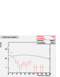
(a) Track Isolation

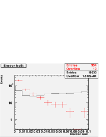
(b) Iso $E_{T}$

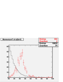
(c) Electron $E_{T}$

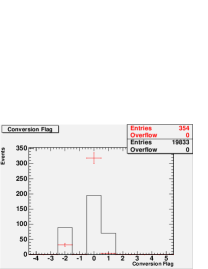
(d) Conversion Flag

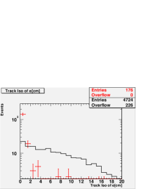
(e) Track Isolation

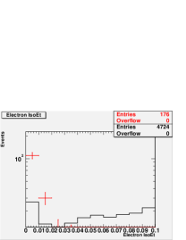
(f) Iso $E_{T}$

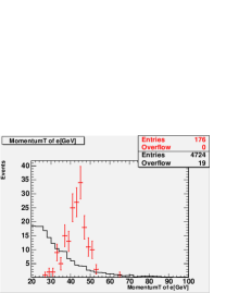
(g) Electron $E_{T}$

(h) Conversion Flag

Figure 10.4: A comparison of distributions from fake ‘electrons’ from the Non-WZ sample(black histogram) and from electrons from tight Z’s (red dots). The top set of plots has no (calorimeter) IsoEt cut applied; the IsoEt cut is applied in the bottom plots. The plot labeled ‘Conversion’ shows the value of the conversion flag, where the meaning is: 0 - not a conversion, 1 - conversion electron, -2 - trident.

           

(a) Track Isolation

(b) Iso $E_{T}$

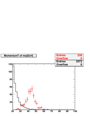
(c) Muon $P_{T}$

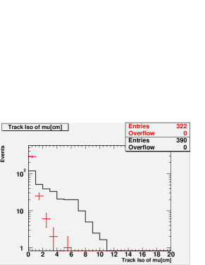
(d) Track Isolation

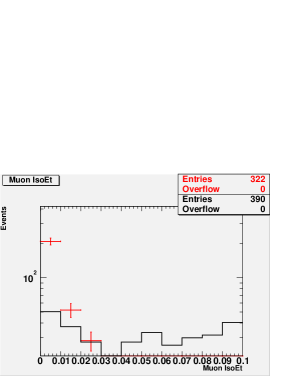
(e) Iso $E_{T}$

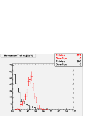
(f) Muon $P_{T}$

Figure 10.5: A comparison of distributions from fake ‘muons’ from the Non-WZ sample(black histogram) and from muons from tight Z’s (red dots). The top set of plots has no (calorimeter) IsoEt cut applied; the IsoEt cut is applied in the bottom plots.

10.2.2 Track Isolation Method

To calculate the backgrounds from fake W’s and fake Z’s in which the lepton comes from a jet, we use the track isolation of the lepton and the samples of good electrons from Z’s and QCD background from the non-WZ sample described above. The procedure is as follows:

• Assume W, Z, $W\gamma$, $Z\gamma$ all have the same underlying event structure, including jets (good assumption to first order in the SM, see for example Figure 10.6).

     

  

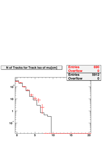
  (a) Number of Tracks in a cone 0.4

  

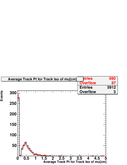
  (b) Average Track ${\rm p}_{\rm T}$ in a cone 0.4

  Figure 10.6: Check of the same underlying event structure assumption: muons from $\mu\mu j$ (red points) vs “golden” Z (black histogram).

• Define 3 samples:

  • $\ell\gamma\mbox{${\rm\not\!E}_{\rm T}$}$ or $ll\gamma$ (signal region)

  • golden-lepton (tight central-central electrons Z${}^{0}\rightarrow e^{+}e^{-}$, tight muons Z${}^{0}\rightarrow\mu^{+}\mu^{-}$)

  • Non-W/Z QCD background

• [0] $N_{TOT}$: Number of events in a signal sample
  Count $N_{TOT}$ events of $\ell\gamma\mbox{${\rm\not\!E}_{\rm T}$}$($ll\gamma$)

• [1] $f_{S}$: fraction of golden leptons with bad track isolation
  From the golden-lepton sample find the fraction $f_{S}$ of golden leptons that have bad track isolation (tiso$>$4).

• [2] $N_{S}^{tiso>4}$: number of signal in a $tiso>4$ region
  $f_{S}\times N_{TOT}$ represents the number of real electrons we will lose by subtracting off electrons with tiso$>$4 in the $\ell\gamma\mbox{${\rm\not\!E}_{\rm T}$}$($ll\gamma$) sample. This has an uncertainty ($\delta f_{S}\times N_{TOT}$) $\Rightarrow$
  $N_{S}^{tiso>4}=f_{S}\times N_{TOT}\pm\delta f_{S}\times N_{TOT}$

• [3] $R_{B}$: ratio of background with good track isolation to the bad track isolation
  From the non-WZ sample find the ratio $R_{B}$ of background with good track tiso ($tiso<2$) to those with bad track tiso ($tiso>4$). We use this to estimate how many of the tiso$<$2 candidates are really QCD background.
  $R_{B}={{Non-WZ^{tiso<2}}\over{Non-WZ^{tiso>4}}}$

• [4] $N_{B}^{tiso>4}$: the number of background with $tiso>4$
  From the $\ell\gamma\mbox{${\rm\not\!E}_{\rm T}$}$($ll\gamma$) sample, the number of background with tiso$>$4 should be the number of candidates with tiso$>$4 minus the expected number of real electrons with tiso$>$4:
  $N_{B}^{tiso>4}=N_{data}^{tiso>4}-N_{S}^{tiso>4}$

• [5] $N_{B}^{tiso<2}$: the number of background with $tiso<2$
  The number of background with $tiso<2$ is
  $N_{B}^{tiso<2}=(R_{B})(N_{B}^{tiso>4})\pm\delta N_{B}^{tiso<2}$

• [6] $N_{B}^{2<tiso<4}$: the number of background with $2<tiso<4$
  From number of background in $tiso>4$ $N_{B}^{tiso>4}$ and number of events in Non-WZ sample with $2<tiso<4$ and $tiso>4$ we estimate number of background with $2<tiso<4$. The number of background with $2<tiso<4$ is
  $N_{B}^{2<tiso<4}=(N_{B}^{tiso>4})\times{{Non-WZ^{2<tiso<4}}\over{Non-WZ^{tiso>4}}}$

• [7] $N_{QCD}$: QCD background
  Resulting Number of QCD background
  $N_{QCD}=N_{B}^{tiso<2}+N_{B}^{2<tiso<4}+N_{B}^{tiso>4}$

10.2.3 Non-W/Z Results

We have used track isolation to make estimates of the non-W backgrounds in the W${}^{\pm}\rightarrow l^{\pm}\nu$ control sample (Section 10.2.5).

Table 10.3 summarizes the numbers of track-isolated and non-track-isolated events in the good electron, non-WZ, and signal samples. In addition, we add numbers of events from W+jet and Z+jet categories, used to estimate jet faking photon background.

The good electrons are heavily track-isolated ($0<tiso<2$); the QCD background ‘electrons’ are predominantly track-non-isolated ($4<tiso$).

	$0~{}GeV<tiso<2~{}GeV$	$2~{}GeV<tiso<4~{}GeV$	$tiso>4~{}GeV$	total
Electrons:
$Z_{tight}^{CC}$	11204	610	534	12348
Non-WZ	1179	870	3709	5758
$e\gamma\mbox{${\rm\not\!E}_{\rm T}$}$	21	2	2	25
$ee\gamma$	35	1	2	38
$ej\mbox{${\rm\not\!E}_{\rm T}$}$	1.98655	0.164143	0.62847	2.77916
$eej$	0.46559	0.0241221	0.0371426	0.526854
Muons:
$Z_{tight}$	5686	190	36	5912
Non-WZ	173	78	93	344
$\mu\gamma\mbox{${\rm\not\!E}_{\rm T}$}$	16	1	0	17
$\mu\mu\gamma$	22	2	0	24
$\mu j\mbox{${\rm\not\!E}_{\rm T}$}$	1.41881	0.0601055	0.0618934	1.54081
$\mu\mu j$	0.264149	0.00932185	0.0318951	0.305366

Table 10.3: The numbers of events that are track-isolated ($0<tiso<2$) versus non-track-isolated ($tiso>4$) for good electrons, QCD background ‘electrons’, and the signal samples. The good electrons are heavily track-isolated; the QCD background ‘electrons’ are predominantly track-non-isolated.

Table 10.6 shows step-by-step calculation of predicted QCD (Non-WZ) backgrounds.

Sample	$f_{S}^{tiso>4}$	$N_{S}^{tiso>4}$	$R_{B}$	$N_{B}^{tiso>4}$	$N_{B}^{tiso<2}$	$N_{B}^{2<tiso<4}$	$N_{B}^{tot}$
$e\gamma\mbox{${\rm\not\!E}_{\rm T}$}$	0.043$\pm$0.0023	1.1$\pm$0.057	0.32$\pm$0.014	0.92$\pm$0.057	0.29$\pm$0.031	0.22$\pm$0.024	1.4$\pm$0.11
$ee\gamma$	0.043$\pm$0.0023	1.6$\pm$0.086	0.32$\pm$0.014	0.36$\pm$0.086	0.11$\pm$0.032	0.084$\pm$0.024	0.55$\pm$0.14
$\mu\gamma\mbox{${\rm\not\!E}_{\rm T}$}$	0.0061$\pm$0.0011	0.1$\pm$0.019	1.9$\pm$0.33	0$\pm$0.019	0$\pm$0.035	0$\pm$0.016	0$\pm$0.069
$\mu\mu\gamma$	0.0061$\pm$0.0011	0.15$\pm$0.026	1.9$\pm$0.33	0$\pm$0.026	0$\pm$0.049	0$\pm$0.022	0$\pm$0.097

Table 10.4: Predicted QCD backgrounds: step-by-step calculation.

Sample	$f_{S}^{tiso>4}$	$N_{S}^{tiso>4}$	$R_{B}$	$N_{B}^{tiso>4}$	$N_{B}^{tiso<2}$	$N_{B}^{2<tiso<4}$	$N_{B}^{tot}$
$e\gamma\mbox{${\rm\not\!E}_{\rm T}$}$	0.043$\pm$0.0023	0.96$\pm$0.05	0.32$\pm$0.014	0.41$\pm$0.05	0.13$\pm$0.022	0.096$\pm$0.017	0.64$\pm$0.089
$ee\gamma$	0.043$\pm$0.0023	1.6$\pm$0.085	0.32$\pm$0.014	0.34$\pm$0.085	0.11$\pm$0.032	0.08$\pm$0.024	0.53$\pm$0.14
$\mu\gamma\mbox{${\rm\not\!E}_{\rm T}$}$	0.0061$\pm$0.0011	0.094$\pm$0.017	1.9$\pm$0.33	0$\pm$0.017	0$\pm$0.031	0$\pm$0.014	0$\pm$0.063
$\mu\mu\gamma$	0.0061$\pm$0.0011	0.14$\pm$0.026	1.9$\pm$0.33	0$\pm$0.026	0$\pm$0.048	0$\pm$0.022	0$\pm$0.096

Table 10.5: Predicted QCD backgrounds: with jet fakes subtracted. Step-by-step calculation.

Sample	$f_{S}^{tiso>4}$	$N_{S}^{tiso>4}$	$R_{B}$	$N_{B}^{tiso>4}$	$N_{B}^{tiso<2}$	$N_{B}^{2<tiso<4}$	$N_{B}^{tot}$
$e\gamma\mbox{${\rm\not\!E}_{\rm T}$}$	0.043$\pm$0.0023	0.84$\pm$0.044	0.32$\pm$0.014	0$\pm$0.044	0$\pm$0.014	0$\pm$0.01	0$\pm$0.068
$ee\gamma$	0.043$\pm$0.0023	1.6$\pm$0.084	0.32$\pm$0.014	0.33$\pm$0.084	0.1$\pm$0.031	0.077$\pm$0.023	0.51$\pm$0.14
$\mu\gamma\mbox{${\rm\not\!E}_{\rm T}$}$	0.0061$\pm$0.0011	0.085$\pm$0.015	1.9$\pm$0.33	0$\pm$0.015	0$\pm$0.028	0$\pm$0.013	0$\pm$0.056
$\mu\mu\gamma$	0.0061$\pm$0.0011	0.14$\pm$0.026	1.9$\pm$0.33	0$\pm$0.026	0$\pm$0.048	0$\pm$0.021	0$\pm$0.095

Table 10.6: Predicted QCD backgrounds: with jet fakes double-subtracted. Step-by-step calculation.

10.2.4 Modified Track Isolation Method

From the jet fake rate we obtain (fake gamma + real W) and (fake gamma + fake W) backgrounds. From Track Isolation Method we obtain (real gamma + fake W) and possibly (fake gamma + fake W).

To summarize, there are three sources of faking $W\gamma$ with either fake gamma and/or fake W:

1. fake gamma + real W (from jet fake rate)

2. fake gamma + fake W (also part of jet fake rate and possibly part of non-W/Z background)

3. real gamma + fake W (from non-W/Z background)

If fake W is a part of non-W/Z background it should contribute to track-non-isolated regions. Real W’s from W+jet should have the same track isolation distribution as W+$\gamma$ (we have performed the checks for all the samples we use, see for example Figure 10.6).

To avoid double counting, we modify Track Isolation Method as follows: we subtract W+jet faking photon contribution from $\ell\gamma\mbox{${\rm\not\!E}_{\rm T}$}$ trackiso regions, we subtract Z+jet faking photon contribution from $\ell\ell\gamma$ trackiso regions. Then we repeat procedure, documented in Section 10.2.2, with these modified $\ell\gamma\mbox{${\rm\not\!E}_{\rm T}$}$ and $\ell\ell\gamma$ numbers (Table 10.6).

To take into account systematic error of 100% for jet faking photon rate (Table 10.6) we repeat these procedure, subtracting W+jet and Z+jet contribution multiplied by 2. Therefore, to avoid double-counting we use background estimates from “Predicted QCD Backgrounds with Jet Fakes Subtracted” (Table 10.6).

Region, GeV	$e\gamma\mbox{${\rm\not\!E}_{\rm T}$}$	$ee\gamma$	$\mu\gamma\mbox{${\rm\not\!E}_{\rm T}$}$	$\mu\mu\gamma$
0-2; 2-$\infty$	1.4$\pm$0.11	0$\pm$0.17	0.58$\pm$0.12	2.1$\pm$0.23
0-2; 4-$\infty$	0.64$\pm$0.09	0.53$\pm$0.14	0$\pm$0.06	0$\pm$0.10
0-2; 5-$\infty$	1.2$\pm$0.09	1.2$\pm$0.14	0$\pm$0.07	0$\pm$0.1
0-2.5; 4.5-$\infty$	0.93$\pm$0.09	0.9$\pm$0.14	0$\pm$0.07	0$\pm$0.1
0-3; 3-$\infty$	0.03$\pm$0.08	0$\pm$0.14	0$\pm$0.08	1.6$\pm$0.2
0-3; 5-$\infty$	1.2$\pm$0.09	1.2$\pm$0.14	0$\pm$0.07	0$\pm$0.1
Final	0.7	0.6	0.3	1.0
	$\pm$0.1(stat)	$\pm$0.1(stat)	$\pm$0.1(stat)	$\pm$0.1(stat)
	$\pm$0.7(sys)	$\pm$0.6(sys)	$\pm$0.3(sys)	$\pm$1.0(sys)

Table 10.7: QCD studies table: estimating the QCD background faking a $\ell\gamma\mbox{${\rm\not\!E}_{\rm T}$}$ or $\ell\ell\gamma$ event. The method uses track isolation and two regions, one at low track-iso and one at high. Leptons from the Z${}^{0}\rightarrow\ell^{+}\ell^{-}$ sample are used to estimate the number of leptons in the high-track-iso region; ‘leptons’ from the non-WZ sample are used to estimate the number of leptons in the low-track-iso region. The first column of the table gives the ranges in GeV for the low and high track-iso regions, respectively. The last line gives the final estimates.

Finally, Non-W/Z backgrounds for $\ell\gamma\mbox{${\rm\not\!E}_{\rm T}$}$ and $\ell\ell\gamma$ signatures are summarized in Table 10.7. Systematic errors are obtained by varying track isolation regions. Further checks for Non-WZ background for W${}^{\pm}\rightarrow e^{\pm}\nu$ and W${}^{\pm}\rightarrow\mu^{\pm}\nu$ are described below in Section 10.2.5.

10.2.5 Non-W/Z background for W${}^{\pm}\rightarrow e^{\pm}\nu$ and W${}^{\pm}\rightarrow\mu^{\pm}\nu$

We have used track isolation to make estimates of the non-WZ backgrounds in the W${}^{\pm}\rightarrow l^{\pm}\nu$ control sample and $\ell\ell\gamma$ and $\ell\gamma\mbox{${\rm\not\!E}_{\rm T}$}$ signal samples. Table 10.8 shows the estimated ‘non-W’ background in the W samples for 5 different track-iso regions. This is for a check- the values are consistent with known QCD backgrounds for W’s [62]. The method uses track isolation and two regions, one at low track-iso and one at high. Leptons from the golden Z sample are used to estimate the number of leptons in the high-track-iso region; ‘leptons’ from the non-WZ sample are used to estimate the number of leptons in the low-track-iso region. The first column of the table gives the ranges in GeV for the low and high track-iso regions, respectively.

Region, GeV	W${}^{\pm}\rightarrow e^{\pm}\nu$	W${}^{\pm}\rightarrow\mu^{\pm}\nu$
0-2; 4-$\infty$	6.5e+02$\pm$6.6e+02	1.8e+03$\pm$7.3e+02
0-3; 5-$\infty$	1.1e+03$\pm$6.5e+02	1.6e+03$\pm$7.2e+02
0-2; 5-$\infty$	1.1e+03$\pm$6.5e+02	1.6e+03$\pm$7.3e+02
0-2; 2-$\infty$	56$\pm$8.3e+02	5.7e+02$\pm$7.7e+02
0-3; 3-$\infty$	4.5e+02$\pm$7.1e+02	1.1e+03$\pm$7e+02

Table 10.8: QCD backgrounds for W’s The method uses track isolation and two regions, one at low track-iso and one at high. Leptons from the golden Z sample are used to estimate the number of leptons in the high-track-iso region; ‘leptons’ from the non-WZ sample are used to estimate the number of leptons in the low-track-iso region. The first column of the table gives the ranges in GeV for the low and high track-iso regions, respectively.

Chapter 11 Systematic Uncertainties

In this chapter we summarize estimates of the systematic uncertainties on the SM predicted rates and on the measured event counts.

The errors are categorised as theoretical (Section 11.1), luminosity (Section 11.2) and experimental (Section 11.3. The contributing effects for the SM predictions we have considered are:

• 7% error is on the total theoretical prediction, including the NLO uncertainties.

• Luminosity: 6%

• Trigger Efficiencies: 2% for muons and 1% for electrons for lepton triggers only. We OR’ing lepton trigger with photon trigger, and therefore this combination of triggers is fully efficient.

• $|$z_vert$|$ $<$ 60: 1%

• Muon ID Efficiencies: 2%

• Electron ID Efficiencies: 1%

• Photons ID Efficiencies: 4%

The systematic uncertainties on the backgrounds are included in the background estimates, discussed in Chapter 9 and Chapter 10. For the SM predictions the total systematic uncertainty is 10.2% for $W\gamma$ and $Z\gamma$ for electrons, and 10.5% for $W\gamma$ and $Z\gamma$ for muons (Chapter 9).

11.1 Theoretical Systematic Uncertainties

Limitations in the theoretical precision of the calculation, result in an uncertainty on the cross-section prediction. The effect of these errors on the cross-section is studied in [7, 41, 83] and is summarized in Table 11.1

Source	%
Factorization Scale	2
PDF	6
K-factor	3
Total	7

Table 11.1: Systematic errors on the $Z\gamma$, $W\gamma$, $Z\gamma\gamma$ and $W\gamma\gamma$ generation

11.1.1 Factorization Scale

The factorization scale is the minimum $Q^{2}$ value calculated [41, 83] for photon emission in the ZGAMMA and WGAMMA programs [70]. This value will affect the maximum $Q^{2}$ value for post generation Pythia fragmentation. The default factorization scale was $\hat{s}$, the square of the collision energy of the event. The cross-section and acceptance were measured using four other values, 2 $\hat{s}$, 3/2 $\hat{s}$, 2/3 $\hat{s}$and 1/2 $\hat{s}$. The greatest variation in the cross-section from the default value of Q2 was 2%.

11.1.2 Parton Density Function Choice

Protons and anti-protons are composite particles. Therefore, any interactions between them must be described using parton density functions (PDF). The PDF describes the energy distributions of the valence quarks, gluons and sea quarks inside the proton/anti-proton.

The PDF chosen for use with ZGAMMA [70] was the CTEQ5L PDF. In order to determine the systematic error from this choice, the LO cross-section is compared to the corresponding predictions calculated from the MRST 72 - 76 PDFs. The MRST cross-sections range between 1.604 and 1.625 $pb^{-1}$ whereas the cross-section using CTEQ5L is 1.72 $pb^{-1}$. The difference between the two was taken to be the systematic error [41, 83], of 6%.

11.1.3 K-factor

The calculated K-factor only takes into account O($\alpha_{s}$) corrections. To take into account higher order corrections, the Q scale in the NLO calculation was varied by factors of 2 and 1/2. A 3% variation in the cross-section calculation was observed, and taken to be a systematic error.

11.2 Luminosity Systematic Uncertainties

The luminosity error is estimated to be 6%, which includes a 4.4% contribution from the acceptance and operation of the luminosity monitor and 4.0% from the theoretical uncertainty on the calculation of the total $\rm p{\bar{p}}$ cross-section [49].

11.3 Experimental Systematic Uncertainties

The sources of experimental systematic errors [7, 41, 83] for the $\ell\gamma+X$ analysis subcategories are summarized in Table 11.2. Jet Fake systematic error is discussed in Section 10.1.1.

Source	%	Central	Plug	CMUP	CMX
Jet Fake	$\approx$100	x	x	x	x
$Z_{0}$ cut eff	1.0	x	x	x	x
photon cut eff	2.0	x	x	x	x
energy scale ($\gamma$)	3.0	x	x	x	x
conversion rate uncertainty	1.5	x	x	x	x
momentum scale ($\mu$)	2.0			x	x
acceptance ($e$)	1.0	x	x
acceptance ($\mu$)	2.0			x	x
central $e$ ID	1.0	x
central $e$ trigger	1.0	x
energy scale ($e$)	1.0	x	x
plue $e$ ID	2.5		x
plug trig eff	1.0		x
plug $e$ vertex eff	1.0		x
plug $e$ track eff	1.5		x
cosmic	0.01			x	x
Cot track reconstruction	0.4	x		x	x
CMUP ID	0.7			x
CMUP reconstruction	0.6			x
CMUP trigger	0.7			x
CMX ID	0.8				x
CMX reconstruction	0.3				x
CMX trigger	0.6				x

Table 11.2: Systematic errors summary for $\ell\gamma$. ’x’ means that channel needs to take into account its systematic uncertainty. Jet Fake systematic error is discussed in Section 10.1.1

Systematic uncertainty on jet faking photon rate is one of the dominating errors. The uncertainty is limited by the statistics for the high-${\rm E}_{\rm T}$ photons, so we expect it to significantly improve with more data. At that point we’ll be dominated by the systematic uncertainty. Therefore, the biggest contribution will be from the SM estimates on $W\gamma$, $Z\gamma$, $W\gamma\gamma$ and $Z\gamma\gamma$ production.

Chapter 12 The $\ell\gamma+X$ Search

This chapter presents the results of the $\ell\gamma+X$ search for the three signatures of interest - $\ell\gamma\mbox{${\rm\not\!E}_{\rm T}$}$, $\ell\ell\gamma$ and $\ell\ell\gamma$.

Section 12.1 describes the ‘analysis subcategories’ established in the Run I analysis [2], and used again here so as to be a priori. Section 12.2 presents the number of events in each analysis subcategory for the $e\gamma+X$, $\mu\gamma+X$, and $\ell\gamma+X$ (the sum of $e+\mu$) samples. Section 12.3 discusses the stability of the observed numbers during the course of the run. The predicted and observed totals for the $\ell\gamma\mbox{${\rm\not\!E}_{\rm T}$}$, $\ell\ell\gamma$ and $\ell\gamma\gamma$ and comparison of observed kinematic distributions to the SM predicted shapes is done in Section 12.4.

12.1 Defining the Event Categories by Topology

Categories of photon-lepton events were defined a priori in a way that characterized the different possibilities for new physics. For each category, the inclusive event total and basic kinematic distributions can be compared with standard model expectations. The decay products of massive particles are typically isolated from other particles, and possess large transverse momentum and low rapidity.

Therefore, inclusive $\ell\gamma$ events are selected by requiring a central tight photon with $\mathrm{E_{T}^{\gamma}}>25$ $GeV$ and a central $e$ or $\mu$ with $\mathrm{E_{T}^{\ell}}>25$ $GeV$. Both signal and control samples are drawn from this $\ell\gamma$ sample (Figures 12.3, 12.1 and  12.2).

Considering the control samples first, from the $\ell\gamma$ sample we select back-to-back events with exactly one photon and one lepton (i.e. $\mbox{${\rm\not\!E}_{\rm T}$}<25~{}GeV$); this is the dominant contribution to the $\ell\gamma$ sample, and has a large Drell-Yan component. A subset of this sample is the ‘Z-like’ sample, which provides the calibration for the probability that an electron radiates and is detected as a photon, as discussed in Section 10.1.2. The remaining back-to-back events are called the Two-Body Events and were not used in this analysis.

All events which either have more than one lepton or photon, or in which the lepton and photon are not back-to-back (and hence the event cannot be a Two-Body event), are classified as ‘Inclusive Multi-Body $\ell\gamma+X$’. These are further subdivided into three categories: $\ell\gamma\mbox{${\rm\not\!E}_{\rm T}$}$ (Section 12.5) (‘Multi-Body $\ell\gamma\mbox{${\rm\not\!E}_{\rm T}$}$ Events’), for which the ${\rm\not\!E}_{\rm T}$ (Section 8.1) is greater than 25 GeV , $\ell\ell\gamma$ (Section 12.6) and $\ell\gamma\gamma$ (Section 12.7) (‘Multi-Photon and Multi-Lepton Events’), and events with exactly one lepton and exactly one photon, which are not back-to-back. The events with exactly one lepton and exactly one photon, which are not back-to-back were not used in the analysis.

12.2 The Number of Events Observed

Figure 12.1 shows the results of this classification for the inclusive electron data sample. We find $508$ $e\gamma$ events, of which $111$ are in the Inclusive Multi-Body category. Of these, $25$ are classified as $e\gamma\mbox{${\rm\not\!E}_{\rm T}$}$ events and $0$ and $19$ as Multi-Photon and Multi-Electron events respectively.

Figure 12.2 shows the results for the inclusive muon sample.We find $66$ $\mu\gamma$ events, of which $41$ are in the Inclusive Multi-Body category. Of these, $17$ are classified as $\mu\gamma\mbox{${\rm\not\!E}_{\rm T}$}$ events and $0$ and $12$ as Multi-Photon and Multi-Muon events.

Figure 12.3 shows the sum of the electron and muon entries in the analysis subcategories. There are $42$ $l\gamma\mbox{${\rm\not\!E}_{\rm T}$}$ events, $0$ Multi-Photon events, and $31$ Multi-Lepton events. It is these categories, shown in red in the figures, that are of particular interest due to the Run I results.

Figure 12.1: Electron-photon sample: the subsets of inclusive $e\gamma$ events analyzed.

Figure 12.2: Muon-photon sample: the subsets of inclusive $\mu\gamma$ events analyzed.

Figure 12.3: Lepton-photon sample: the subsets of inclusive $\ell\gamma$ events analyzed.

12.3 Stability of the Event Rates versus Run Number

This sub-section looks at the rate for the analysis subcategories as a function of run number. We use the same eight luminosity bins used to check the stability of the control samples, described in Section 4.1. We see no obvious problems, although the statistics are low. Figure 12.4 shows the rates in events/$pb^{-1}$ for the $\ell\ell\gamma$ and $\ell\gamma\mbox{${\rm\not\!E}_{\rm T}$}$ signal subcategories in each run segment in the muon channel; Figure 12.5 does the same for the electron channel.

   

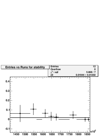
(a) $\ell\ell\gamma$

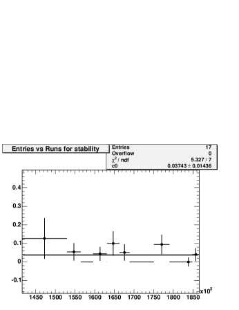
(b) $\ell\gamma\mbox{${\rm\not\!E}_{\rm T}$}$

Figure 12.4: Stability plots for the muon channels of the rate in events per $pb^{-1}$ for the 8 run segments (see Section 4.1) for: a) $\ell\ell\gamma$, and b) $\ell\gamma\mbox{${\rm\not\!E}_{\rm T}$}$.

   

(a) $\ell\ell\gamma$

(b) $\ell\gamma\mbox{${\rm\not\!E}_{\rm T}$}$

Figure 12.5: Stability plots for the electron channels of the rate in events per $pb^{-1}$ for the 8 run segments (see Section 4.1) for: a) $\ell\ell\gamma$, and b) $\ell\gamma\mbox{${\rm\not\!E}_{\rm T}$}$.

12.4 Results

In this section we summarize the predicted and observed totals for the $\ell\gamma\mbox{${\rm\not\!E}_{\rm T}$}$, $\ell\ell\gamma$ and $\ell\gamma\gamma$ searches. We compare observed kinematic distributions to the SM predicted shapes.

12.5 $\ell\gamma\mbox{${\rm\not\!E}_{\rm T}$}$ Search

The predicted and observed totals for the $\ell\gamma\mbox{${\rm\not\!E}_{\rm T}$}$ search are shown in Table 12.1. We observe $42$ $\ell\gamma\mbox{${\rm\not\!E}_{\rm T}$}$ events compared to the expectation of $37.3\pm 5.4$ events.

Lepton+Photon+${\rm\not\!E}_{\rm T}$ Events
SM Source	$e\gamma\mbox{${\rm\not\!E}_{\rm T}$}$	$\mu\gamma\mbox{${\rm\not\!E}_{\rm T}$}$	$(e+\mu)\gamma\mbox{${\rm\not\!E}_{\rm T}$}$
$W^{\pm}\gamma$	13.70$\pm$1.89	8.84$\pm$1.35	22.54$\pm$2.80
$Z^{0}\kern-2.5pt/\kern-1.49994pt\gamma^{*}+\gamma$	1.16$\pm$0.40	4.49$\pm$0.64	5.65$\pm$1.03
$W^{\pm}\gamma\gamma,Z^{0}\kern-2.5pt/\kern-1.49994pt\gamma^{*}\kern-1.79993pt+\kern-1.79993pt\gamma\gamma$	0.14$\pm$0.02	0.18$\pm$0.02	0.32$\pm$0.03
$W^{\pm}\gamma,Z^{0}\kern-2.5pt/\kern-1.49994pt\gamma^{*}\kern-1.79993pt+\kern-1.79993pt\gamma\kern-1.79993pt\rightarrow\kern-1.79993pt\tau\gamma$	0.71$\pm$0.18	0.26$\pm$0.08	0.97$\pm$0.22
$W^{\pm}$+Jet faking $\gamma$	2.8$\pm$2.8	1.6$\pm$1.6	4.4$\pm$4.4
$Z^{0}\kern-2.5pt/\kern-1.49994pt\gamma^{*}\kern-1.79993pt\rightarrow\kern-1.79993pte^{+}e^{-},e\kern-1.79993pt\rightarrow\kern-1.79993pt\gamma$	2.45$\pm$0.33	-	2.45$\pm$0.33
Jets faking $\ell+\mbox{${\rm\not\!E}_{\rm T}$}$	0.7$\pm$0.7	0.3$\pm$0.3	1.0$\pm$0.8
Total SM
Prediction	21.7$\pm$3.4	15.7$\pm$2.2	37.3$\pm$5.4
Observed
in Data	25	17	42

Table 12.1: A comparison of the numbers of events predicted by the standard model(SM) and the observations for the $\ell\gamma\mbox{${\rm\not\!E}_{\rm T}$}$ search. The SM predictions for the search are dominated by $W\gamma$ production, respectively [68, 71, 69]. Other contributions come from $Z\gamma$ production, from the tri-boson processes $W\gamma\gamma$ and $Z\gamma\gamma$, leptonic $\tau$ decays, and misidentified leptons, photons, or ${\rm\not\!E}_{\rm T}$.

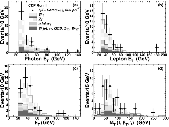
Figure 12.6: Distributions for the events in the $\ell\gamma\mbox{${\rm\not\!E}_{\rm T}$}$ sample (points) in a) the ${\rm E}_{\rm T}$ of the photon; b) the ${\rm E}_{\rm T}$ of the lepton; c) the missing transverse energy, ${\rm\not\!E}_{\rm T}$; and d) the transverse mass of the $\ell\gamma\mbox{${\rm\not\!E}_{\rm T}$}$ system. The histograms show the expected SM contributions, including estimated backgrounds from misidentified photons and leptons.

There is no significant excess in the $\ell\gamma\mbox{${\rm\not\!E}_{\rm T}$}$ signature. Figure 12.6 shows the observed distributions summed over the $e\gamma\mbox{${\rm\not\!E}_{\rm T}$}$ and $\mu\gamma\mbox{${\rm\not\!E}_{\rm T}$}$ events in a) the ${\rm E}_{\rm T}$ of the photon; b) the ${\rm E}_{\rm T}$ of the lepton; c) the missing transverse energy, ${\rm\not\!E}_{\rm T}$; and d) the transverse mass of the $\ell\gamma\mbox{${\rm\not\!E}_{\rm T}$}$ system, where $\rm{M_{T}}=[{(\rm E_{T}^{\ell}+E_{T}^{\gamma}+\mbox{${\rm\not\!E}_{\rm T}$})^{2}}$ - $({\vec{E}_{T}^{\ell}}+{\vec{E}_{T}^{\gamma}}+{\not\!\!\vec{E}_{T}})^{2}]^{1/2}$.

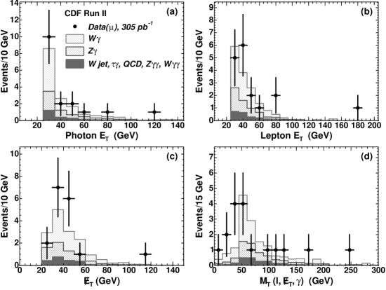
Figure 12.7: Distributions for the events in the $\mu\gamma\mbox{${\rm\not\!E}_{\rm T}$}$ sample (points) in a) the ${\rm E}_{\rm T}$ of the photon; b) the ${\rm E}_{\rm T}$ of the muon; c) the missing transverse energy, ${\rm\not\!E}_{\rm T}$; and d) the transverse mass of the $\ell\gamma\mbox{${\rm\not\!E}_{\rm T}$}$ system. The histograms show the expected SM contributions, including estimated backgrounds from misidentified photons and leptons.

The predicted and observed kinematic distributions for $\mu\gamma\mbox{${\rm\not\!E}_{\rm T}$}$ are compared in Figure 12.7. The distributions for $e\gamma\mbox{${\rm\not\!E}_{\rm T}$}$ signature are compared in Figure 12.8.

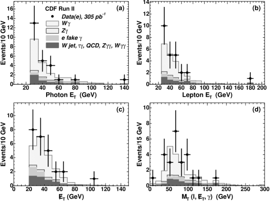
Figure 12.8: Distributions for the events in the $e\gamma\mbox{${\rm\not\!E}_{\rm T}$}$ sample (points) in a) the ${\rm E}_{\rm T}$ of the photon; b) the ${\rm E}_{\rm T}$ of the electron; c) the missing transverse energy, ${\rm\not\!E}_{\rm T}$; and d) the transverse mass of the $\ell\gamma\mbox{${\rm\not\!E}_{\rm T}$}$ system. The histograms show the expected SM contributions, including estimated backgrounds from misidentified photons and leptons.

The additional plots of the identification variables for $e\gamma\mbox{${\rm\not\!E}_{\rm T}$}$ and $\mu\gamma\mbox{${\rm\not\!E}_{\rm T}$}$ are available in Section LABEL:lgmet_plots.

12.6 $\ell\ell\gamma$ Search

The predicted and observed totals for the $\ell\ell\gamma$ search are shown in Table 12.2. We observe $31$ $\ell\ell\gamma$ events compared to the expectation of $23.0\pm 2.7$ events.

Multi-Lepton + Photon Events
SM Source	$ee\gamma$	$\mu\mu\gamma$	$ll\gamma$
$Z^{0}\kern-2.5pt/\kern-1.49994pt\gamma^{*}+\gamma$	12.50$\pm$1.53	7.81$\pm$0.88	20.31$\pm$2.40
$Z^{0}\kern-2.5pt/\kern-1.49994pt\gamma^{*}+\gamma\gamma$	0.24$\pm$0.03	0.12$\pm$0.02	0.36$\pm$0.04
$Z^{0}\kern-2.5pt/\kern-1.49994pt\gamma^{*}+$Jet faking $\gamma$	0.3$\pm$0.3	0.2$\pm$0.2	0.5$\pm$0.5
$Z^{0}\kern-2.5pt/\kern-1.49994pt\gamma^{*}\kern-1.79993pt\rightarrow\kern-1.79993pte^{+}e^{-},e\kern-1.79993pt\rightarrow\kern-1.79993pt\gamma$	0.23$\pm$0.09	-	0.23$\pm$0.09
Jets faking $\ell+\mbox{${\rm\not\!E}_{\rm T}$}$	0.6$\pm$0.6	1.0$\pm$1.0	1.6$\pm$1.2
Total SM
Prediction	13.9$\pm$1.7	9.1$\pm$1.4	23.0$\pm$2.7
Observed
in Data	19	12	31

Table 12.2: A comparison of the numbers of events predicted by the standard model(SM) and the observations for the $\ell\ell\gamma$ search. The SM predictions for the search are dominated by $Z\gamma$ production [68, 71, 69]. Other contributions come from the tri-boson process $Z\gamma\gamma$, and misidentified leptons or photons.

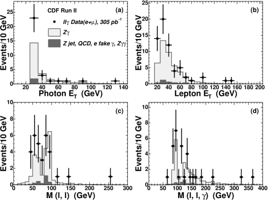
Figure 12.9: Distributions for the events in the $\ell\ell\gamma$ sample (points) in a) the ${\rm E}_{\rm T}$ of the photon; b) the ${\rm E}_{\rm T}$ of the leptons (two entries per event); c) the 2-body mass of the dilepton system; and d) the 3-body mass $m_{\ell\ell\gamma}$. The histograms show the expected SM contributions.

The $\ell\ell\gamma$ search criteria select $31$ events ($19$ $ee\gamma$ and $12$ $\mu\mu\gamma$) of the $574$ $\ell\gamma$ events. No $e\mu\gamma$ events are observed. Figure 12.9 shows the observed distributions in a) the ${\rm E}_{\rm T}$ of the photon; b) the ${\rm E}_{\rm T}$ of the leptons; c) the 2-body mass of the dilepton system; and d) the 3-body mass $m_{\ell\ell\gamma}$. For the $Z\gamma$ process occurring via initial state radiation, the dilepton invariant mass $m_{\ell\ell}$ distribution is peaked around the $Z^{0}$-pole. For the final state radiation, the three body invariant mass $m_{\ell\ell\gamma}$ distribution is peaked about the $Z^{0}$-pole.

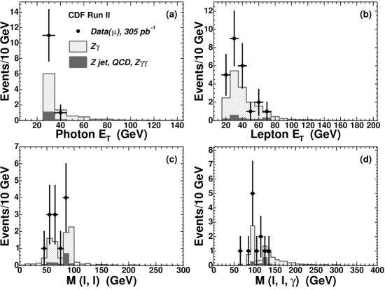
Figure 12.10: Distributions for the events in the $\mu\mu\gamma$ sample (points) in a) the ${\rm E}_{\rm T}$ of the photon; b) the ${\rm E}_{\rm T}$ of the muons (two entries per event); c) the 2-body mass of the dimuon system; and d) the 3-body mass $m_{\mu\mu\gamma}$. The histograms show the expected SM contributions.

The predicted and observed kinematic distributions for $\mu\mu\gamma$ are compared in Figure 12.10. The distributions for $ee\gamma$ signature are compared in Figure 12.11. The dominant contribution for the $ee\gamma$ and $\mu\mu\gamma$ signatures is from the SM $Z\gamma$ production.

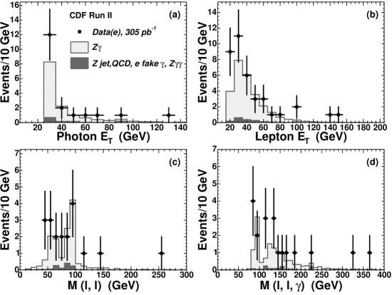
Figure 12.11: Distributions for the events in the $ee\gamma$ sample (points) in a) the ${\rm E}_{\rm T}$ of the photon; b) the ${\rm E}_{\rm T}$ of the electrons (two entries per event); c) the 2-body mass of the dielectron system; and d) the 3-body mass $m_{ee\gamma}$. The histograms show the expected SM contributions.

We do not expect events with large ${\rm\not\!E}_{\rm T}$ in the $\ell\ell\gamma$ sample, based on the SM backgrounds; the Run I $ee\gamma\gamma\mbox{${\rm\not\!E}_{\rm T}$}$ event was of special interest in the context of supersymmetry [18, 19] due to the large value of ${\rm\not\!E}_{\rm T}$ (55 $\pm$ 7 $GeV$). Figure 12.12 shows the distributions in ${\rm\not\!E}_{\rm T}$ for the $\mu\mu\gamma$ and $ee\gamma$ subsamples of the $\ell\ell\gamma$ sample. No events are observed with $\mbox{${\rm\not\!E}_{\rm T}$}>25$ $GeV$.

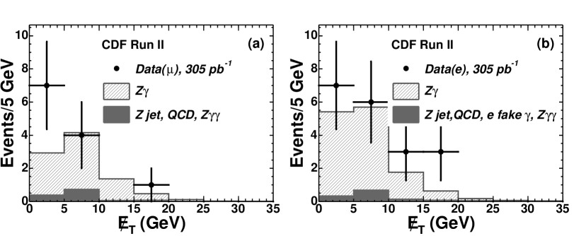
Figure 12.12: Distributions in missing transverse energy ${\rm\not\!E}_{\rm T}$ observed in the inclusive search for a) $\mu\mu\gamma$ events and b) $ee\gamma$ events. The histograms show the expected SM contributions.

The additional plots of the identification variables for $ee\gamma$ and $\mu\mu\gamma$ are available in Section LABEL:llg_plots.

12.7 $\ell\gamma\gamma$ Search

The predicted and observed totals for the $\ell\gamma\gamma$ search are shown in Table 12.3. We do not observe any $\ell\gamma\gamma$ candidate events compared to the expectation of $0.23\pm 0.080$ events.

Multi-Photon + Lepton Predicted Events
SM Source	$e\gamma\gamma$	$\mu\gamma\gamma$	$\l\gamma\gamma$
$W^{\pm}\gamma\gamma$	$0.0067\pm 0.0014$	$0.0037\pm 0.00095$	$0.010\pm 0.0017$
$Z^{0}\gamma\gamma$	$0.015\pm 0.0017$	$0.011\pm 0.0014$	$0.026\pm 0.0022$
$Z^{0}\gamma$, $e\kern-1.79993pt\rightarrow\kern-1.79993pt\gamma$	$0.193\pm 0.080$	-	$0.193\pm 0.080$
Total SM
Prediction	$\bf 0.22\pm 0.080$	$\bf 0.015\pm 0.0022$	$\bf 0.23\pm 0.080$
Observed
in Data	$0$	$0$	$0$

Table 12.3: The predicted number of multi-body events with additional photons in $305pb^{-1}$ from Standard Model sources, and the numbers of events observed. The $Z\gamma\gamma$ and $W\gamma\gamma$ predictions are from MadGraph. The “$Z^{0}\gamma$, $e\rightarrow\gamma$” prediction is taken from the data.

Conclusions

In conclusion, we have searched for physics beyond the Standard Model in a channel in which new phenomena due to supersymmetry or extra dimensions, for example, could well appear. In particular, we have repeated the Run I CDF search for inclusive lepton + photon production, a final state in which both a very rare event appeared and also in which there seemed to be an excess over SM predictions. The new analysis, the subject of this thesis, was done specifically with the same kinematic requirements as the Run I search, but with a significantly larger data sample and a higher collision energy.

We conclude that the excess in the $\ell\gamma\mbox{${\rm\not\!E}_{\rm T}$}$ signature in Run I of 2.7 sigma was at least largely a statistical fluctuation. If the Run I ratio of the number of $\ell\gamma\mbox{${\rm\not\!E}_{\rm T}$}$ events observed to the number expected, 16/7.6, had held up, the “2.7 $\sigma$ excess” in this channel observed in Run I would have resulted in an observation of 78$\pm$11 events when $37.3\pm 5.4$ are expected in the Run II repeat of the analysis, versus the $42$ events observed.

We find that the numbers of events in the $\ell\gamma\mbox{${\rm\not\!E}_{\rm T}$}$ and $\ell\ell\gamma$ subsamples of the $\ell\gamma+X$ sample agree with the SM predictions. We find no events like the $ee\gamma\gamma\mbox{${\rm\not\!E}_{\rm T}$}$ candidate event of Run I, and, even more generally, observe no $\ell\ell\gamma$ events with anomalous large ${\rm\not\!E}_{\rm T}$ or with multiple photons. We have no explanation for the Run I $ee\gamma\gamma\mbox{${\rm\not\!E}_{\rm T}$}$ event, and nothing we have measured leads us to believe that is background.

However, we still find that in the $\ell\gamma\mbox{${\rm\not\!E}_{\rm T}$}$ signature in the Run II data the number of observed events is higher than predicted, although the excess is now slight. It is possible that the leading-order + K-factor theoretical calculations of the diboson $W\gamma$ and $Z\gamma$ channels, which contain many diagrams including initial state radiation, are not precise enough for the precision we have now reached.

Alternatively, or perhaps in addition, this analysis has observed a small number of events on the ‘tails’ of the kinematic distributions, in regions we expect few SM events. These events contribute to the observation of more events than expected in the $\ell\gamma\mbox{${\rm\not\!E}_{\rm T}$}$ signature, much as the $ee\gamma\gamma\mbox{${\rm\not\!E}_{\rm T}$}$ event contributed to the excess in the Run I search. Whether these are very rare backgrounds or something new will require yet more data.

The Fermilab plan is to have a factor of 10-20 more data than presented here by the end of Run II of the Tevatron. The increased statistics will require an improved understanding of backgrounds as well as better SM predictions. In particular the estimate of the rate for a jet to be misidentified as a photon is limited now by the statistics for high-${\rm E}_{\rm T}$ photons; we expect the estimate will significantly improve with more data.

In summary, while it would have been very exciting to find physics beyond the Standard Model, we found no more $ee\gamma\gamma\mbox{${\rm\not\!E}_{\rm T}$}$ events in a much larger sample than in Run I, and the Run I excess in $\ell\gamma\mbox{${\rm\not\!E}_{\rm T}$}$ became less significant rather than more. However, we have conclusively settled a question that generated much interest in the theoretical community. The channels we have investigated will remain interesting, and the techniques we have developed and the knowledge gained will be useful for similar searches at the LHC.

Appendix A Appendices

A.1 List Of Lepton-Photon Events

	$\gamma$			$\ell$					$\ell\gamma$		${\rm\not\!E}_{\rm T}$
run/event	${\rm E}_{\rm T}$	$\phi$	$\eta$	type	${\rm p}_{\rm T}$	$\phi$	$\eta$	T	$\Delta\phi$	$m_{\ell\gamma}$	${\rm\not\!E}_{\rm T}$	$\phi$
179043/12444345	+29.13	-0.88	0.07	CMUP	27.16	-2.18	-0.20	1	1.30	34.60	27.67	1.36
178602/5535619	25.97	-1.29	1.04	CMUP	33.03	0.29	-0.24	1	1.58	58.37	30.98	2.96
178816/108292	+31.28	1.78	0.77	CMUP	77.49	-1.35	-0.20	1	3.12	110.7	34.17	3.06
178855/422245	+31.27	0.48	0.57	CMX	42.14	0.05	0.91	1	0.43	17.13	31.94	2.39
151843/1584392	+25.40	-1.55	0.10	CMUP	41.13	3.12	-0.21	1	1.61	47.87	48.05	0.76
151870/1255798	+79.18	-0.24	-0.28	CMX	62.62	2.32	0.80	1	2.56	158.8	27.78	-1.77
153739/175671	+28.20	-1.41	0.78	CMUP	41.18	-1.26	0.26	1	0.15	16.61	32.21	-0.42
155895/6336800	+55.41	2.30	-0.29	CMUP	52.70	-0.06	0.24	1	2.35	104.5	34.93	-1.76
160230/4222557	+52.97	1.22	1.02	CMX	49.38	0.83	0.66	1	0.39	25.13	43.43	-2.12
162686/2327952	+50.31	0.10	-0.23	CMUP	79.31	0.86	0.33	1	0.75	58.83	44.12	-2.52
166406/10446136	+119.8	0.86	0.05	CMX	25.17	-2.62	0.78	1	2.81	114.3	110.2	-2.26
166653/3270001	+32.07	-0.03	0.43	CMUP	26.39	0.63	0.51	1	0.66	18.81	48.83	-2.89
164274/2876183	+35.10	-1.17	0.19	CMX	38.78	-2.49	0.70	1	1.31	49.92	45.23	1.37
166008/3466824	42.82	-0.13	0.90	CMUP	184.1	2.05	-0.47	1	2.18	201.6	35.74	2.54
164386/2366320	25.30	0.84	0.45	CMUP	35.43	0.34	0.39	1	0.49	14.67	39.06	-2.23
186145/10202075	+27.36	-2.31	-0.33	CMUP	26.58	2.81	0.29	1	1.16	32.93	47.40	0.25
185332/13796632	+28.88	2.72	0.44	CMX	38.52	-2.61	0.92	1	0.96	33.46	57.47	0.14

Table A.1: List of muon + photon + ${\rm\not\!E}_{\rm T}$ events. ${\rm E}_{\rm T}$, ${\rm p}_{\rm T}$, ${\rm\not\!E}_{\rm T}$ and $m_{\ell\gamma}$ are in $GeV$. Column “T” shows if an event has been triggered by the high-${\rm E}_{\rm T}$ muon trigger. “+” in front of $\mathrm{E_{T}^{\gamma}}$ value means that an event has been triggered by the high-${\rm E}_{\rm T}$ photon trigger.

	$\gamma$			$\ell$					$\ell\gamma$		${\rm\not\!E}_{\rm T}$
run/event	${\rm E}_{\rm T}$	$\phi$	$\eta$	type	${\rm p}_{\rm T}$	$\phi$	$\eta$	T	$\Delta\phi$	$m_{\ell\gamma}$	${\rm\not\!E}_{\rm T}$	$\phi$
177371/273794	25.24	-1.91	-0.39	CMP	40.37	2.10	-0.20	-	2.27	58.09	7.84	1.33
				CMUP	34.51	-0.49	-0.39	1	1.42	38.43
179043/9452199	+28.91	-0.03	0.29	CMX	29.72	-2.47	0.79	1	2.44	57.61	5.55	2.79
				CMX	20.95	1.30	-0.64	1	1.34	37.71
152507/1700045	+34.62	0.99	-0.96	CMX	65.31	-3.00	-0.73	1	2.30	87.55	7.18	-0.82
				CMUP	27.43	0.06	-0.47	1	0.93	31.31
153345/1348276	+35.05	-0.13	-0.65	CMX	25.75	-3.13	0.78	0	3.00	75.63	1.85	-2.04
				CMUP	21.63	0.27	-0.37	1	0.40	12.46
154175/360663	+32.17	-1.23	0.12	CMP	29.45	0.76	0.43	-	1.99	52.65	3.67	-2.65
				CMX	28.42	2.99	0.75	1	2.06	55.60
155895/2377214	+26.58	-0.21	0.70	CMUP	29.76	-1.33	0.33	1	1.12	31.49	16.3	-3.08
				CMIO	23.10	0.00	-0.54	-	0.22	39.49
156089/1783191	+27.40	-2.75	-0.84	CMX	39.87	0.50	-0.73	1	3.03	66.16	4.24	-0.63
				CMUP	25.97	-2.71	-0.38	1	0.04	13.48
161330/3293805	+27.42	-0.22	0.32	CMUP	42.07	2.56	0.11	1	2.77	66.85	8.00	2.89
				CMIO	21.70	-0.70	0.63	-	0.48	13.49
162479/90695	+26.73	-0.29	-0.63	CMX	46.39	1.95	-0.91	1	2.24	64.14	3.76	2.27
				CMIO	41.69	-1.37	-1.00	-	1.08	36.36
162238/185410	+28.27	-2.27	-0.24	CMUP	59.06	-0.12	-0.26	0	2.14	71.82	0.49	0.15
				CMP	40.10	1.83	0.47	-	2.19	66.24
164261/192043	+25.70	-0.68	-0.20	CMUP	37.11	2.82	0.47	1	2.79	65.35	2.71	2.21
				CMUP	20.54	-0.13	-0.25	1	0.55	12.42
167955/33039	+26.68	-2.66	0.58	CMUP	55.97	-0.04	0.31	1	2.63	75.52	4.43	0.32
				CMIO	34.75	2.61	0.60	-	1.01	29.41

Table A.2: List of multi-muon + photon events. ${\rm E}_{\rm T}$, ${\rm p}_{\rm T}$, ${\rm\not\!E}_{\rm T}$ and $m_{\ell\gamma}$ are in $GeV$. Column “T” shows if an event has been triggered by the high-${\rm E}_{\rm T}$ muon trigger. “+” in front of $\mathrm{E_{T}^{\gamma}}$ value means that an event has been triggered by the high-${\rm E}_{\rm T}$ photon trigger.

	$\gamma$			$\ell$					$\ell\gamma$		${\rm\not\!E}_{\rm T}$
run/event	${\rm E}_{\rm T}$	$\phi$	$\eta$	type	${\rm p}_{\rm T}$	$\phi$	$\eta$	T	$\Delta\phi$	$m_{\ell\gamma}$	${\rm\not\!E}_{\rm T}$	$\phi$
178537/410195	+54.36	-3.09	0.97	TCEM	31.41	-1.11	0.53	1	1.98	71.53	67.39	0.60
178677/5534996	+38.69	-0.13	0.39	TCEM	37.70	1.27	0.07	0	1.40	50.56	49.60	-2.45
178758/3669012	+53.70	-2.28	-0.76	TCEM	27.63	-0.46	-0.86	1	1.82	60.93	40.55	1.38
178785/12963076	+58.01	-3.09	-0.62	TCEM	28.12	-2.63	0.77	1	0.46	63.80	56.56	0.30
151515/2273934	+34.33	-3.12	-0.18	TCEM	51.43	0.86	0.67	1	2.30	85.51	37.75	-1.54
152602/728988	+27.60	3.00	-0.19	TCEM	57.76	-0.67	-0.80	1	2.61	81.15	34.44	1.37
156083/1091219	+35.04	2.13	-0.19	TCEM	33.24	1.07	0.37	1	1.06	39.69	65.11	-1.57
161170/427847	+26.24	-2.29	-0.27	TCEM	25.04	0.44	-0.15	1	2.73	50.25	34.92	-2.44
163064/10108920	+81.04	-1.15	-0.12	TCEM	70.13	1.64	1.07	1	2.80	178.7	29.38	1.58
163431/1462399	+31.00	-0.54	-0.40	TCEM	27.76	0.03	-0.32	1	0.57	16.82	57.92	2.90
163526/14750	+25.41	-2.06	-0.46	TCEM	29.98	1.34	-0.54	0	2.88	54.76	29.75	-1.00
167299/670904	+27.78	2.29	-0.77	TCEM	26.16	1.92	-0.43	1	0.37	13.47	43.32	-1.04
167849/2063706	+48.13	3.12	0.89	TCEM	41.48	1.28	-0.14	1	1.84	84.77	42.78	-0.70
168599/3868597	+32.85	0.89	0.72	TCEM	53.58	-1.71	-0.66	1	2.60	101.9	28.62	2.19
183752/4059116	+46.67	-0.50	-0.28	TCEM	45.66	2.00	0.76	1	2.51	101.0	27.34	-2.60
184762/1221041	+30.45	2.64	0.47	TCEM	59.61	2.95	0.75	1	0.31	18.43	101.3	-0.32
183965/5394458	+36.76	0.45	0.68	TCEM	33.65	-1.72	0.80	1	2.17	62.32	28.56	2.48
184519/1108274	+33.70	-2.64	-0.50	TCEM	41.63	-0.84	0.18	1	1.81	64.29	35.83	2.10
184453/1736470	+28.81	1.89	0.35	TCEM	53.71	2.93	0.49	1	1.04	39.35	36.29	-1.22
184778/6449604	+28.14	-0.85	-0.71	HCEM	176.9	-0.09	-0.59	1	0.77	53.58	26.61	-3.07
184067/336957	+142.1	2.20	0.38	TCEM	68.80	-3.11	-0.45	1	0.97	125.0	32.88	-0.44
184868/4710858	+37.63	-0.32	-0.55	TCEM	47.46	-3.05	0.31	1	2.73	90.83	33.97	1.18
185176/11940	+25.94	1.24	-0.91	TCEM	44.78	2.44	0.44	1	1.19	61.29	41.11	-1.32
184778/345250	+28.03	2.82	0.13	TCEM	33.77	1.54	-0.57	1	1.28	42.98	26.55	-1.21
185848/2995941	+43.42	-2.57	0.50	TCEM	43.14	0.65	1.07	1	3.06	90.03	28.09	0.61

Table A.3: List of electron + photon + ${\rm\not\!E}_{\rm T}$ events. ${\rm E}_{\rm T}$, ${\rm p}_{\rm T}$, ${\rm\not\!E}_{\rm T}$ and $m_{\ell\gamma}$ are in $GeV$. TCEM stands for Tight CEM electron. Column “T” shows if an event has been triggered by the high-${\rm E}_{\rm T}$ electron trigger. “+” in front of $\mathrm{E_{T}^{\gamma}}$ value means that an event has been triggered by the high-${\rm E}_{\rm T}$ photon trigger.

Table A.4: List of multi-electron + photon events. ${\rm E}_{\rm T}$, ${\rm p}_{\rm T}$, ${\rm\not\!E}_{\rm T}$ and $m_{\ell\gamma}$ are in $GeV$. TCEM stands for Tight CEM Electron. LCEM stands for Loose CEM Electron. HCEM stands for Tight100 CEM Electron. EAST stands for Phoenix East Plug Electron, WEST stands for Phoenix West Plug Electron. Column “T” shows if an event has been triggered by the high-${\rm E}_{\rm T}$ electron trigger. “+” in front of $\mathrm{E_{T}^{\gamma}}$ value means that an event has been triggered by the high-${\rm E}_{\rm T}$ photon trigger.

	$\gamma$			$\ell$					$\ell\gamma$		${\rm\not\!E}_{\rm T}$
run/event	${\rm E}_{\rm T}$	$\phi$	$\eta$	type	${\rm p}_{\rm T}$	$\phi$	$\eta$	T	$\Delta\phi$	$m_{\ell\gamma}$	${\rm\not\!E}_{\rm T}$	$\phi$
178602/3018939	+25.72	2.74	-0.89	TCEM	60.24	-0.68	-0.74	1	2.85	78.14	5.95	-1.56
				TCEM	32.77	2.23	0.65	1	0.52	51.37
178852/3194148	+94.25	-2.93	0.64	TCEM	101.7	0.58	0.65	1	2.77	192.5	6.18	-1.46
				LCEM	31.52	-1.14	0.65	1	1.79	84.90
153074/1339595	+25.54	-0.33	-0.18	TCEM	76.89	2.87	-1.02	1	3.08	95.67	16.3	1.31
				TCEM	38.95	-1.34	-0.99	1	1.01	39.36
160346/1528176	+45.61	-0.82	-0.87	TCEM	50.34	-3.12	-1.00	1	2.30	87.71	19.7	1.84
				LCEM	24.53	0.81	-0.94	1	1.63	48.68
155394/2469758	+27.80	-1.77	-0.28	WEST	52.56	1.12	1.82	1	2.89	123.4	1.62	1.45
				TCEM	29.65	-2.30	0.80	1	0.53	35.45
155996/1191192	+37.75	1.21	-0.64	TCEM	66.64	2.81	-1.06	0	1.60	75.27	7.42	-1.72
				EAST	19.33	-0.27	-1.37	0	1.49	41.49
161830/69435	+135.0	-0.19	-0.57	HCEM	138.5	3.07	0.82	1	3.02	340.2	12.	2.50
				LCEM	26.95	1.91	-0.16	1	2.11	107.5
162396/1323030	+27.61	0.55	-0.99	TCEM	39.96	-2.81	-0.95	1	2.92	66.01	2.94	1.13
				LCEM	20.18	0.15	-0.39	1	0.40	15.82
164844/6642760	+26.85	-0.66	-0.07	TCEM	57.45	-2.92	0.88	1	2.26	80.95	9.50	1.53
				TCEM	41.01	0.54	0.98	1	1.20	52.39
166038/6509526	+31.01	2.27	0.36	TCEM	27.90	-1.89	0.96	1	2.13	55.19	4.32	1.68
				LCEM	22.41	-0.13	-0.15	1	2.40	50.98
167623/4691216	+27.49	1.92	0.70	TCEM	28.78	1.70	0.21	1	0.21	13.31	10.4	-1.32
				LCEM	23.13	-1.49	-0.72	1	2.88	62.58
167866/443088	+67.15	-1.26	-0.29	TCEM	148.1	1.73	0.05	1	2.99	201.8	17.1	1.47
				TCEM	99.93	-1.29	0.54	1	0.03	70.28
183913/878106	+30.10	-0.75	-0.92	TCEM	42.48	2.21	0.61	1	2.96	91.99	4.56	2.77
				EAST	17.65	-1.26	-1.57	1	0.50	20.09
184519/3570367	+27.58	2.43	0.44	TCEM	35.08	-0.80	-0.18	1	3.05	65.14	9.03	-2.57
				WEST	16.02	0.97	1.28	1	1.46	33.13
185037/1000257	+33.05	-1.15	-0.22	EAST	51.01	1.45	-1.35	1	2.60	92.97	2.53	-1.22
				TCEM	34.93	-2.46	0.93	1	1.30	59.26
185075/1540099	+64.57	2.85	0.17	TCEM	59.86	-0.71	0.48	1	2.71	123.0	12.2	0.48
				WEST	18.92	1.35	1.78	1	1.51	78.68
185281/13145621	+32.43	-1.69	-0.95	TCEM	44.60	0.95	-0.40	1	2.64	77.33	5.00	-0.63
				TCEM	33.45	2.93	-0.52	1	1.66	51.20
185634/4852157	+37.10	1.98	0.83	TCEM	28.27	-1.85	0.56	1	2.45	61.58	1.85	-0.98
				TCEM	25.95	-0.12	0.36	1	2.10	55.73
186145/10988173	+31.88	1.18	0.14	TCEM	27.08	-2.73	0.58	1	2.37	56.00	1.76	-0.85
				LCEM	22.91	-1.20	-0.68	1	2.38	55.12

A.2 Additional $\ell\gamma\mbox{${\rm\not\!E}_{\rm T}$}$ Plots

In this section we present additional plots of the identification variables for $\mu\gamma\mbox{${\rm\not\!E}_{\rm T}$}$ and $e\gamma\mbox{${\rm\not\!E}_{\rm T}$}$ signatures.

A.2.1 Additional $\mu\gamma\mbox{${\rm\not\!E}_{\rm T}$}$ Plots

       

   

A.2.2 Additional $e\gamma\mbox{${\rm\not\!E}_{\rm T}$}$ Plots

       

       

A.3 Additional $\ell\ell\gamma$ Plots

In this section we present additional plots of the identification variables for $\mu\mu\gamma$ and $ee\gamma$ signatures.

A.3.1 Additional $\mu\mu\gamma$ Plots

       

       

       

     

A.3.2 Additional $ee\gamma$ Plots

       

       

A.4 Stability Plots for $Zj$ and $Wj$

To check electron and muon identification in events with an extra object (such as a photon in the signal channel) we plot the rate for $Zj$ and $Wj$ in the 8 bins of luminosity (Table 4.1) in Figure LABEL:zjwj_stability.figure.

       

A.5 CMX vs CMUP muons: Comparison of Isolation Variables

We have checked that muons that go into the CMX system have the same isolation properties as CMUP muons. Figure LABEL:cmx_vs_cmup.figure shows the distributions in calorimeter isolation, relative track isolation (total ${\rm p}_{\rm T}$ of tracks in a cone in $\eta-\varphi$ space of radius $R=0.4$ around the muon track divided by ${\rm p}_{\rm T}^{muon}$) and absolute track isolation for Z${}^{0}\rightarrow\mu^{+}\mu^{-}$ and W${}^{\pm}\rightarrow\mu^{\pm}\nu$ events.

           

A.6 Fake Electrons from Photon Conversions

There are three dominant sources of fake electrons: a) photons from $\pi^{0}$, $\eta$ and other mesons, that convert into asymmetric $e^{+}e^{-}$ pairs in the material before the COT volume, b) charged hadrons in jets that either interact in the electromagnetic volume of the calorimeter or overlap with a $\pi^{0}$ or secondary photon in the jet, and c) electrons from the decay of heavy flavor ($b$, $c$, and maybe even $s$). We estimated these backgrounds in Section 10.2 by studying the total ${\rm p}_{\rm T}$ of tracks in a cone in $\eta-\varphi$ space of radius $R=0.4$ around the lepton track.

We consider fake electrons from photon conversions below. Electrons coming from photon conversion are identified by conversion algorithm, which looks for couple of opposite sign tracks with $|\Delta xy|<$0.2 cm and $|\Delta cot(\theta)|<$0.04.

For each electron a conversion flag is tested. We define if the electron is flagged as coming from a conversion ($\gamma\rightarrow e^{+}e^{-}$) or from trident events where a conversion is caused by a bremsstrahlung photon ($e\rightarrow e\gamma,\gamma\rightarrow e^{+}e^{-}$). We study same-sign events in Z${}^{0}\rightarrow e^{+}e^{-}$ sample and then check how many of them contain electrons tagged as conversions or tridents.

           

 

Figure LABEL:zeess.figure shows the distributions for same-sign and opposite-sign $e^{+}e^{-}$ pairs. The invariant mass of the same-sign electrons is shifted with respect to the invariant mass of Z${}^{0}\rightarrow e^{+}e^{-}$ (Figure LABEL:zeess.figure, a). We observe similar behavior (shift in invariant mass distribution) in the Z${}^{0}\rightarrow e^{+}e^{-}$ MC as in data (Figure LABEL:ztop2i_zee_z_mass.figure).

To develop an understanding of the conversion cut for the candidate events, we summarize the same-sign events in Z${}^{0}\rightarrow e^{+}e^{-}$ sample. Out of $199$ events in this sample only $21$ are not tagged as either a conversion electron or a trident. We find that we have $5$ same sign muon events, which is comparable to $21$ non-conversion/trident same-sign electron events.

Z${}^{0}\rightarrow e^{+}e^{-}$ same sign	199
Z${}^{0}\rightarrow e^{+}e^{-}$ SS, one conversion	44
Z${}^{0}\rightarrow e^{+}e^{-}$ SS, one trident	106
Z${}^{0}\rightarrow e^{+}e^{-}$ SS, two conversions (CC)	4
Z${}^{0}\rightarrow e^{+}e^{-}$ SS, two tridents (TT)	11
Z${}^{0}\rightarrow e^{+}e^{-}$ SS trident + conversion (TC)	13
Z${}^{0}\rightarrow e^{+}e^{-}$ SS neither conversion/trident	21

A.7 Checking the $\mu\mu\gamma$ and $\mu\gamma\mbox{${\rm\not\!E}_{\rm T}$}$ for Additional Backgrounds

We have used a number of techniques, described below, to look for additional backgrounds in the $\mu\mu\gamma$ and $\mu\gamma\mbox{${\rm\not\!E}_{\rm T}$}$ samples.

Same-Sign Leptons to Estimate Jets Faking one or More Leptons

We used results from Ref. [84] on the numbers of same-sign (SS) and other-sign (OS) muon pairs in the dimuon sample. The expected background from SS muon pairs to $\mu\mu\gamma$ is calculated as follows.

First we obtain the ratio of W+1 jet events to OS events, x, expected in the dimuon sample: x = SS/OS $\times$ 1.51$\pm$0.05. For the $\mu\mu$ sample ratio of SS/OS is of order of 0.05% and therefore x=0.1%. In the $\mu\mu\gamma$ sample we have 12 OS events, and therefore the expected background from W+1 jet is negligible, 0.1% $\times$ 12 = 0.012$\pm$0.001 events.

Decays in flight of Low Momentum $K^{\pm}$ Faking a High-Momentum Muon

A low-momentum hadron, not in an energetic jet, can decay to a muon forming a “kink” between the hadron and muon trajectories (Figure LABEL:dif_scatch.figure). In this case a high-momentum track may be reconstructed from the initial track segment due to the hadron and the secondary track segment from the muon. A kaon that decays before the COT volume results in a muon whose momentum is correctly measured; a kaon that decays after the COT is itself correctly measured. These contributions are included in the total background estimate (see Section 10.2).

The contribution from this background is estimated by identifying tracks consistent with a “kink” in the COT. We count the number of times that, proceeding radially along a COT track, a “hit” in the n+1 layer of sense-wires is on the other side of the fitted track from the hit in the nth layer. Real tracks will have hits distributed on both sides of the fit, and will therefore have many “transitions”. A mis-measured track from a 5-$GeV$ $K^{+}$ (for example), on the other hand, will consist of two intersecting low-momentum arcs fit by a high momentum track, and will have a small number of transitions [85].

Figure LABEL:ztight_mu_transitions_good_mu_transitions shows the number of transitions in muons in the Z${}^{0}\rightarrow\mu^{+}\mu^{-}$ control sample, and in a sample enriched in hadron decays by selecting events with a large $\mbox{${\rm\not\!E}_{\rm T}$}>25~{}GeV$, at least one jet and muon that have large impact parameter $d_{0}>0.2~{}$cm. Figure LABEL:dif_mumug_mugmet.figure shows the number of transitions for muon tracks with and without silicon hits. The red curve is the distribution for the muons from Z${}^{0}\rightarrow\mu^{+}\mu^{-}$ sample. Decays-in-flight have a distribution that peaks much lower, with few events above 30 transitions. We see no evidence that any of these tracks are DIF muons.

       

$\mu\mu\gamma$, $\mu\gamma\mbox{${\rm\not\!E}_{\rm T}$}$ Cosmics Background

For this we invert cosmic cut, and require the event to be tagged as cosmic [59]. We processed the unstripped high-${\rm p}_{\rm T}$ muon sample with this inverted requirement and found no $\mu\mu\gamma$ or $\mu\gamma\mbox{${\rm\not\!E}_{\rm T}$}$ candidate events.

In addition we scanned our $\mu\gamma\mbox{${\rm\not\!E}_{\rm T}$}$ and $\mu\mu\gamma$ candidate events with CDF Run II Event Display (Section 3) and made sure that none of them look like beam halo or cosmics events.

Bibliography

- [1] S.L. Glashow, Nucl. Phys. 22 588, (1961); S. Weinberg, Phys. Rev. Lett. 19 1264, (1967); A. Salam, Proc. 8th Nobel Symposium, Stockholm, (1979).
- [2] D. Acosta et al. (CDF Collaboration), Phys. Rev. D 66, 012004 (2002); hep-ex/0110015.
- [3] D. Acosta et al. (CDF Collaboration), Phys. Rev. Lett. 89, 041802 (2002); hep-ex/0202004.
- [4] A. Abulencia et al. (CDF Collaboration), Phys. Rev. Lett. 97, 031801 (2006), hep-ex/0605097.
- [5] A.Loginov for the CDF Collaboration. Search for New Physics in Photon Final States. Eur.Phys.J. C 46, Supplement 2, pp. 21-31 (2006).
- [6] A.Loginov for the CDF Collaboration. Search for New Physics in Lepton + Photon + X Events with 929 of Collisions at = 1.96 . Proceedings of Crimea Conference, Ukraine, 16-23 Sep 2006. FERMILAB-CONF-06-403-E.
- [7] D. Acosta et al. (CDF Collaboration), Phys. Rev. Lett. 94, 041803 (2005).
- [8] A.Loginov for the CDF Collaboration. Search for New Physics in Photon Final States (SUSY 2005, Durham). FERMILAB-CONF-05-598-E; hep-ex/0604036, 2005.
- [9] H. Frisch. Collider Physics Experiments. Proceedings of the Twenty First Lake Louise Winter Institute, 2006.
- [10] CDF Run II Event Display Code is available at: http://cdfkits.fnal.gov/CdfCode/source/RootEventDisplay/ http://cdfkits.fnal.gov/CdfCode/source/RootMods/.
- [11] D. Litvintsev, A. Loginov, I. Shreyber. The CDF Run II Event Display Users Manual. CDF7054; http://evd.fnal.gov, 2006.
- [12] A. Loginov, Y. C. Chen for CDF Collaboration. The CDF Run II Live Events. ”Live Events” Page, http://evd.fnal.gov/online, 2006.
- [13] CDF Run II Event Display Team: James Bellinger (UoW, Madison) Jong-young Chung (OSU) YeonSei Chung (UR) Elena Gerchtein (ITEP) Robert Harr (WSU) Konstantin Kotelnikov (ITEP) Dmitry Litvintsev (ITEP, Project Leader 1998-2001) Andrey Loginov (ITEP, Project Leader 2001-2007) Akiya Miyamoto (KEK) Pasha Murat (Fermilab) Carsten Rott (Purdue) Kurt Rinnert (University of Karlsruhe) Tony Vaiciulis (UR) Elena Vataga (New Mexico University) .
- [14] Sally Dawson John F. Gunion (Editor) Howard E. Haber, Gordon Kane. Higgs Hunter’s Guide. Westview Press, 2000.
- [15] P. Langacker, Proceedings of PASCOS 90 symposium, eds. P.Nath and S.Reucroft (World Scientific, Singapore, 1990); J. Ellis, S. Kelley, and D.V. Nanopoulos, Phys. Lett. B249, 441 (1990); U. Amaldi, W. de Boer, and H. Frstenau, Phys. Lett. B260, 447 (1991); P. Langacker and M.-X. Luo, Phys. Rev. D44, 817 (1991) .
- [16] K. Lane and E. Eichten. Natural topcolor–assisted technicolor. Physics Letters B, 352:382, 1995.
- [17] N. Arkani-Hamed and S. Dimopoulos and G. Dvali. Phys. Lett. B, 429:263, 1998.
- [18] S. Ambrosanio, G.L. Kane, G.D. Kribs, S.P. Martin, and S. Mrenna, Phys. Rev. D 55, 1372 (1997).
- [19] K. Sridhar Phys. Rev. Lett. 89 011801 (2002); hep-ph/0111014. B.C. Allanach, S. Lola.
- [20] L. Susskind. Phys. Rev. D, D20, 1979.
- [21] H.P. Nilles, Phys. Rep. 110, 1 (1984); H.E. Haber and G.L. Kane, Phys. Rep. 117, 75 (1985).
- [22] For a summary, see: B. C. Allanach et al. (Les Houches working group). Les Houches ’Physics at TeV colliders 2005’ Beyond the standard model working group: Summary report.
- [23] D. J. H. Chung, L. L. Everett, G. L. Kane, S. F. King, J. D. Lykken and L. T. Wang, “The soft supersymmetry-breaking Lagrangian: Theory and applications,” Phys. Rept. 407, 1 (2005) hep-ph/0312378. The gravitino is very light, typically a few MeV.
- [24] S. P. Martin. A Supersymmetry Primer, in Perspectives on Supersymmetry, G. Kane, editor. Singapore: World Scientific, 1998. hep-ph/9709356.
- [25] S. Ambrosanio, G. L. Kane, G. D. Kribs, S. P. Martin and S. Mrenna, Phys. Rev. Lett. 76, 3498 (1996).
- [26] S. Ambrosanio, G. L. Kane, G. D. Kribs, S. P. Martin and S. Mrenna. hep-ph/9607414, 1996.
- [27] D. Acosta et al. (CDF Collaboration), Phys. Rev. Lett. 94, 101802 (2005).
- [28] D. Toback, Ph.D. thesis, University of Chicago, 1997.
- [29] J. Berryhill, Ph.D. thesis, University of Chicago, 2000.
- [30] T. Affolder et al. (CDF Collaboration), Phys. Rev. D 65, 052006 (2002).
- [31] F. Abe et al. (CDF Collaboration), Phys. Rev. D 59, 092002 (1999); hep-ex/9806034.
- [32] F. Abe et al., Phys.Rev.Lett 81, 1791 (1998); hep-ex/9801019.
- [33] G. Aubrecht et al. Cockcroft-Walton pre-accelerator. Contemporary Physics Education Project, http://www.lbl.gov/abc/wallchart/teachersguide/pdf/Chap11.pdf.
- [34] C. W. Schmidt. The fermilab 400-mev linac upgrade. Presented at 1993 Particle Accelerator Conference (PAC 93), Washington, DC, 17-20 May 1993.
- [35] Fermilab Beam Division. Main Injector at Tevatron. Technical Report http://www-bd.fnal.gov/runII/index.html.
- [36] F. Abe et al. (CDF Collaboration), Nucl. Instrum. Methods A 271, 387 (1988).
- [37] A. Affolder et al., Nucl. Instrum. Methods A 526, 249 (2004).
- [38] A. Sill et al., Nucl. Instrum. Methods A 447, 1 (2000); A. Affolder et al., Nucl. Instrum. Methods A 453, 84 (2000); C.S. Hill, Nucl. Instrum. Methods A 530, 1 (2000).
- [39] L. Balka et al., Nucl. Instrum. Meth. A267, 272 (1988).
- [40] S. Bertolucci et al., Nucl. Instrum. Meth. A267, 301 (1988).
- [41] H. Hayward, Ph.D. thesis, University of Liverpool, 2005.
- [42] M. G. Albrow et al., Nucl. Instrum. Meth. A480, 524 (2002).
- [43] F. Abe et al. Technical report.
- [44] CDF Collaboration. CDF Run II Muon Chambers. http://www-cdfonline.fnal.gov/cdf_muon/chambers.html.
- [45] T. Dorigo et al. Nuclear Instruments and Methods in Physics Research A, Vol 461, 1, 2001.
- [46] D. Acosta et al., Nucl. Instrum. Meth. A518:605-608, 2004.
- [47] D. Acosta et al. The CDF Cherenkov luminosity monitor. Nuclear Instruments and Methods in Physics Research Section A, Vol 461, Issues 1-3, p540-544, 2001.
- [48] E811 Collaboration. A Measurement of the Proton Anti-Proton Total Cross Section at S**(1/2) = 1.8 TeV. Phys.Lett.B445:419-422, 1999.
- [49] S. Klimenko, J. Konigsberg, T. M. Liss. Averaging of the inelastic crosssections measured by the CDF and E811 experiments. Fermilab-FN-0741.
- [50] A. Bhatti et al., The Beam Shower Counters for Run II, CDF Note 5247.
- [51] M. Goncharov, D. Toback et al., submitted to NIM.
- [52] R. Brun, F. Rademakers. ROOT Framework. Technical Report http://root.cern.ch, 1995-2006.
- [53] R. Kennedyet al., The CDF Run II Event Data Model, Proceedings of CHEP 2000.
- [54] UC CDF Physics Group. The description of the UCNtuple package is available at http://hep.uchicago.edu/cdf/flatntuple. The data and MC sets are listed at http://hep.uchicago.edu/cdf/datasets. 2004.
- [55] S. Levy and C. Pilcher. Personal Communication.
- [56] A. Bhatti et al., Nucl. Instrum. Methods A 566, 375 (2006); hep-ex/0510047.
- [57] D. Acosta et al. (CDF Collaboration), Phys. Rev. D 71, 051104 (2005); hep-ex/0501023.
- [58] V. Martin, High pt muons, recommended cuts and efficiencies for release 5.3.1, CDF Note 7031, 2005; High-Pt Muon ID Cuts and Efficiencies for use with 5.3.1 Data and 5.3.3 MC. We use muon selection cuts which are identical to the standard cuts, with the exception that the impact parameter cut and the cuts on fiducial distance (x-fid, z-fid) are not applied to maximize acceptance. We reject muons from the CMP ’bluebeam’ region for run154449. We also reject muons from the CMX ’keystone’ or ’miniskirt’ regions before the October 2004 shutdown (run 186598).
- [59] A. Taffard, Run II Cosmic Ray Tagger, CDF Note 6100, 2003; A. Taffard, Run II Cosmic Ray Tagger Performance, CDF Note 6255, 2003. We use the COT-based cosmic rejection in CosmicFinderModule and check if COT-based cosmic rejection bit in a cosmic bitword is equal to 1 (cosmic&0x004000).
- [60] L. Beitler. Talk given to the W+Jets Meeting, Oct. 10, 2003.
- [61] Top Group MC Samples. http://www-cdf.fnal.gov/danielw/topmc5/; we used ztop0i Z and ztop2i Z MC samples.
- [62] D. Acosta et al. First measurements of inclusive W and Z cross sections from Run II of the Tevatron collider. Phys. Rev. Lett., 94:091803, 2005.
- [63] C. Hill, J. Incandela, and C. Mills, Electron Identification in Offline Release 5.3, CDF Note 7309, 2005. We use central electron selection cuts which are identical to the standard cuts, with the exception that the CES fiducial requirement and the conversion cut are not applied.
- [64] T. Nelson, R. Snider, D. Stuart. Forward Electron Tracking with the PhoenixMods Package. CDF Note 6278, CDF, 2003.
- [65] P. J. Wilson. Calorimeter Isolation and Lateral Shower Leakage for Photons and Electrons. CDF Note 4170, CDF, 1997.
- [66] G. Veramendi. Personal Communication.
- [67] Y. Ishizawa, J. Nielsen. Trigger Efficiencies for High Et Electrons. CDF Note 7401, CDF, 2005.
- [68] T. Stelzer and W. F. Long, Comput. Phys. Commun. 81, 357 (1994); F. Maltoni and T. Stelzer, JHEP 302, 27 (2003); hep-ph/0208156. We designate the production of lepton pairs through the Drell-Yan process, including both the and amplitudes, as in signatures such as . We use version v3.2.
- [69] A. Pukhov et al.; hep-ph/9908288; E. Boos et al. (The comphep Collaboration), Nucl. Instrum. Methods A 534, 250, (2004); hep-ph/0403113. We use version v4.1.10.
- [70] U. Baur and S. Mrenna. Monte carlo event generator program. http://www.hep.anl.gov/theory/mrenna/sources/uli.uu.
- [71] U. Baur, T. Han, and J. Ohnemus, Phys. Rev. D 48, 5140 (1993); J. Ohnemus, Phys. Rev. D 47, 940 (1993).
- [72] S. Tsuno, A. S. Thompson. A CDF-interface module for Les Houches Accords. CDF Note 6333, CDF, 2003.
- [73] T. Sjostrand, Comput. Phys. Commun. 82 (1994) 74; S. Mrenna, Comput. Phys. Commun. 101 (1997) 232. We use version v6.216. .
- [74] D. Benjamin, A. Goshaw, B. Heinemann and others. Theoretical Predictions of and Production in Run II. CDF Note 6619, CDF, 2004.
- [75] H. Frisch, C. Smith. Predicted Cross Sections for W+Photon and Z+Photon Production. CDF Note 6057, CDF.
- [76] H. Frisch. Appendix A to CDF6057; Final MadGraph , , and Datasets. CDF Note 7523, CDF.
- [77] U. Baur, T. Han and J. Ohnemus, Phys. Rev. D 48, 5140 (1993); U. Baur, T. Han and J. Ohnemus, Phys. Rev. D 57, 2823 (1998); hep-ph/9710416; and U. Baur, private communication. Both the and K-factors are fixed at 1.36 for generated masses below 76 and for generated masses below 86 . Above the poles the K-factors grow with to be 1.62 and 1.53 at for and , respectively.
- [78] H. Frisch, A. Loginov. Search for lepton-photon events. CDF Note 7040, CDF, 2005. We used CDF offline version 4.11.2 both for DATA and MC.
- [79] H. Frisch, A. Loginov, S. Tsuno. and MC MadGraph and Baur Samples. CDF Note 8116, CDF, 2006. To generate final , , and samples we used CDF offline version 5.3.3.
- [80] R. Culbertson, R. Field, H. Frisch, A. Goshaw, B. Heinemann, M. Kirby, A. Loginov, S. Mrenna, P. Murat, S. Tsuno, U. K. Yang. Pythia Settings for Generating , , , Monte Carlo. SM Matching. CDF Note 8126, CDF, 2006.
- [81] H. Hayward, B. Heinemann, The Probability of a Jet Faking an Isolated Photon, CDF Note 6363, 2003; H. Hayward, B. Heinemann, Update on the Measurement of the Probability of a Jet Faking an Isolated Photon, CDF Note 6838, 2004.
- [82] S. Kopp. Measurement of the Ratio R = ) in Collisions at = 1800 GeV. Thesis, CDF, 1994.
- [83] M. Kirby. Measurement of Production in Proton-Antiproton Collisions at root-s = 1.96 TeV. Thesis.
- [84] J. Nachtman and M. Schmitt. Sliding qT Ratio - Muon Channel. CDF Note 7560, CDF, 2005.
- [85] A. Paramonov. Personal Communication.