Measurement of $\rm K^{0}_{\mu 3}$  form factors

Abstract

This paper reports on a new high precision measurement of the form factors of the $\rm K_{L}\rightarrow~{}\pi^{\pm}~{}\mu^{\mp}~{}\nu_{\mu}$  decay. The data sample of about 2.3$\times 10^{6}$ events was recorded in 1999 by the NA48 experiment at CERN. Studying the Dalitz plot density we measured a linear, $\lambda^{{}^{\prime}}_{+}=(20.5\pm 2.2_{stat}\pm 2.4_{syst})\times 10^{-3}$, and a quadratic, $\lambda^{{}^{\prime\prime}}_{+}=(2.6\pm 0.9_{stat}\pm 1.0_{syst})\times 10^{-3}$ term in the power expansion of the vector form factor. No evidence was found for a second order term for the scalar form factor; the linear slope was determined to be $\lambda_{0}=(9.5\pm 1.1_{stat}\pm 0.8_{syst})\times 10^{-3}$. Using a linear fit our results were: $\lambda_{+}=(26.7\pm 0.6_{stat}\pm 0.8_{syst})\times 10^{-3}$ and, $\lambda_{0}=(11.7\pm 0.7_{stat}\pm 1.0_{syst})\times 10^{-3}$.
A pole fit of the form factors yields: $m_{V}=(905\pm 9_{stat}\pm 17_{syst})$ MeV/c² and $m_{S}=(1400\pm 46_{stat}\pm 53_{syst})$ MeV/c².

, , , , , , , , , , , , , , , , , , , , , , , , , , , , , , , , , , , , , , , , , ,

, , , , , , , , , , , , , , , , , , , , , , , , , , , , , , , , , , , , , , , , , , , , , , , , , , , , , , , , , , , , , , , , , , , , , , , , , , , , , , , , , , ,

1 Introduction

Since long ago [1]  $\rm K_{\ell 3}$  decays ($\rm K_{L}\rightarrow~{}\pi^{\pm}~{}\ell^{\mp}~{}\nu,~{}\ell=e,\mu$) have offered the opportunity to test several features of the electroweak interactions such as the V-A structure of weak currents, current algebra and the predictions of chiral perturbation theory. These decays have been the object of a renewed interest both on the experimental and theoretical side since they provide the cleanest [2] way to extract the CKM matrix element $|V_{\it us}|$. $\rm K_{\ell 3}$ decays give access to the product $f_{+}(0)$$|V_{\it us}|$, where $f_{+}(0)$, the vector form factor at zero momentum transfer, has to be determined by theory. The recent calculations at $\mathcal{O}(p^{6})$ [3] in the framework of chiral perturbation theory show how $f_{+}(0)$ could be experimentally constrained from the slope and the curvature of the scalar form factor $f_{0}$ of the $\rm K_{\mu 3}$ decay. In addition, the form factors are needed to calculate the phase space integrals which are another ingredient for the determination of $|V_{\it us}|$. Finally, very recently it has been pointed out [4] how a precise measurement of the value of $f_{0}$ at the Callan–Treiman point [5] could provide a clean test of a small admixture of right handed quark currents (RHCs) coupled to the standard W boson.
Until recently, the experimental knowledge [6] on $\rm K_{\ell 3}$ form factors was mainly based on a certain number of old measurements dating back to the seventies. The slopes obtained from $\rm K_{\mu 3}$ decays were less precise than those determined in $\rm K_{e3}$ decays, and a large difference between the results from charged and neutral kaon decays was present. This difference was more pronounced for the slope $\lambda_{0}$ where, in addition, the situation was confused also by the presence of negative values. Very recent high precision experiments [7, 8, 9, 10, 11] provided a more accurate determination of these quantities with values smaller than the old PDG averages and agreement between $\rm K^{0}$ and $\rm K^{\pm}$ measurements has been established. Furthermore, evidence for a quadratic term in the vector form factor was found, at the level of about 2 $\sigma$, by ISTRA+ in $\rm K_{e3}^{-}$ and by KLOE in $\rm K_{e3}$  decays. A cleaner indication came also from KTeV, both in $\rm K_{e3}$  and $\rm K_{\mu 3}$  decays, with a significance of about 3 $\sigma$.
This paper reports on a new high statistics measurement of $\rm K_{\mu 3}$ form factors. Following this introduction Sec. 2 recalls the formalism about the $\rm K_{\mu 3}$ decays, Sec. 3 describes the experimental set–up, Sec. 4 reports about the analysis, and Sec. 5 delineates the fitting procedure and the treatment of the systematic error.

2 The $\rm K_{L}\rightarrow~{}\pi^{\pm}~{}\mu^{\mp}~{}\nu_{\mu}$ decay

Only the vector current contributes to $\rm K_{\mu 3}$ decays. As a result the matrix element can be written in terms of two dimensionless form factors $f_{\pm}$ :

$${\mathfrak{M}}=\frac{G}{\sqrt{2}}~{}V_{us}~{}\left[f_{+}(t)\left(P_{K}+P_{\pi}\right)^{\mu}\bar{u}_{\ell}\gamma_{\mu}(1+\gamma_{5})u_{\nu}+f_{-}(t)~{}m_{\ell}\bar{u}_{\ell}(1+\gamma_{5})u_{\nu}\right],$$ (1)

where $P_{K}$ and $P_{\pi}$ are the kaon and pion four momenta, respectively, $\bar{u}_{\ell}$ and $u_{\nu}$ are the lepton spinors, $m_{\ell}$ is the lepton mass and $t=(P_{K}-P_{\pi})^{2}=m_{K}^{2}+m_{\pi}^{2}-2P_{K}\cdot P_{\pi}=q^{2}$ is the square of the four–momentum transfer to the lepton pair. The form factor $f_{-}(t)$ is related to a scalar term proportional to the lepton mass and can be measured only in $\rm K_{\mu 3}$ decays.
The determination of the form factors in this analysis is based on a study of the Dalitz plot density which can be parametrized [1] as:

$$\rho(E_{\mu}^{*},E_{\pi}^{*})={dN^{2}(E_{\mu}^{*},E_{\pi}^{*})\over dE_{\mu}^{*}~{}dE_{\pi}^{*}}\propto Af_{+}^{2}(t)+Bf_{+}(t)f_{-}(t)+Cf_{-}^{2}(t),$$ (2)

where A, B and C are kinematical terms:

$$A =m_{K}(2E_{\mu}^{*}E_{\nu}^{*}-m_{K}E_{\pi}^{{}^{\prime}})+m_{\mu}^{2}(1/4~{}E^{{}^{\prime}}_{\pi}-E_{\nu}^{*}),$$

$$B =m_{\mu}^{2}(E_{\nu}^{*}-1/2~{}E_{\pi}^{{}^{\prime}}),$$

$$C =1/4~{}m_{\mu}^{2}E_{\pi}^{{}^{\prime}}.$$

$E_{\mu}^{*},E_{\pi}^{*}$ are the muon and pion energy in the kaon center of mass (CMS) respectively. For the neutrino we have $E_{\nu}^{*}=m_{K}-E_{\mu}^{*}-E_{\pi}^{*}$ and $E_{\pi}^{{}^{\prime}}$ is defined as:

$$E_{\pi}^{{}^{\prime}}=E_{\pi}^{*Max}-E_{\pi}^{*}=\frac{m_{K}^{2}+m_{\pi}^{2}-m_{\mu}^{2}}{2m_{K}}-E_{\pi}^{*}.$$

In an alternative parametrization one can define the form factor $f_{0}(t)$:

$$f_{0}(t)=f_{+}(t)+{t\over(m_{K}^{2}-m_{\pi}^{2})}~{}f_{-}(t).$$ (3)

This parametrization is preferred because $f_{+}$ and $f_{0}$ are related to the vector ($1^{-}$) and scalar ($0^{+}$) exchange to the lepton system, respectively and are less correlated than in the previous case. The expansion in powers of $t$ of the form factors is often stopped at the linear term:

$$f_{\pm,0}(t)=f_{\pm,0}(0)~{}\left(\rule{0.0pt}{14.22636pt}1+\lambda_{\pm,0}~{}t/m_{\pi}^{2}\right).$$ (4)

The assumption that $f_{+}$ and $f_{0}$ are linear in $t$ implies that $f_{+}(0)=f_{0}(0)$ so that $f_{-}$ does not diverge at $t=0$.
The form (4) is usually adopted as consequence of the smallness of data samples from the past experiments rather than on physical motivations. Nowadays, with higher statistics, it is becoming customary to search for a second order term in the form factors expansion:

$$f_{+,0}(t)=f_{+}(0)~{}\left[\rule{0.0pt}{14.22636pt}1+\lambda^{{}^{\prime}}_{+,0}~{}t/m_{\pi}^{2}+\frac{1}{2}~{}\lambda^{{}^{\prime\prime}}_{+,0}~{}(t/m_{\pi}^{2})^{2}\right].$$ (5)

The weak interaction of hadron systems at low energies can also be described in terms of couplings of mesons to the weak gauge bosons (pole model, meson dominance [12]). In this framework the form factors acquire a physical meaning since they can be related to the exchange of the lightest $\rm K^{*}$ resonances which have spin–parity $1^{-}$/$0^{+}$ and mass $m_{V}$/$m_{S}$, respectively:

$$f_{+}(t)=f_{+}(0)~{}\frac{m^{2}_{V}}{m^{2}_{V}-t};~{}~{}~{}~{}~{}~{}~{}~{}~{}~{}~{}~{}~{}~{}f_{0}(t)=f_{+}(0)~{}\frac{m^{2}_{S}}{m^{2}_{S}-t}.$$ (6)

Recently new parametrizations of the vector [13] and scalar [4] form factors based on dispersion relations subtracted twice have been proposed:

$$f_{+}(t)=f_{+}(0)\exp\Bigl{[}\frac{t}{m^{2}_{\pi}}(\Lambda_{+}+H(t))\Bigr{]};~{}~{}~{}~{}~{}f_{0}(t)=f_{+}(0)\exp\Bigl{[}\frac{t}{(m_{K}^{2}-m_{\pi}^{2})}(\ln C-G(t))\Bigr{]},$$ (7)

here $\Lambda_{+}$ is a slope parameter and $\ln C=\ln[f_{0}(m_{K}^{2}-m_{\pi}^{2})]$ is the logarithm of the value of the scalar form factor at the Callan–Treiman point. For the dispersive integrals $H(t)$ and $G(t)$ accurate polynomial approximations have been derived.

3 Experimental set–up

For the measurement reported here the data were taken during a dedicated run period in September 1999. A pure $\rm K_{L}$ beam was produced by 450 GeV/c protons from the CERN SPS hitting a beryllium target. The decay region was contained in a 90 m long evacuated tube and was located 126 m downstream the target after the last of three collimators.
The NA48 detector was originally designed for a precise measurement of direct CP violation in the neutral kaon decays to two pions. A detailed description can be found in [14]; only the main components relevant for this measurement are described here:
Magnetic Spectrometer.  It was contained in a helium tank kept at atmospheric pressure and consisted of four drift chambers and a magnet. Each chamber had four views (x, y, u, v) each of which had two planes of sense wires. The spatial resolution per projection was 100 $\mu$m and the time resolution was 0.7 ns. The magnet, placed between the second and the third chamber, was a dipole with a transverse momentum kick of 265 MeV/c. The momentum resolution of the spectrometer was ($p$ in GeV/c):

$$\frac{\sigma_{p}}{p}=0.48\%\oplus 0.009~{}p\%.$$

Hodoscope.  Located downstream of the spectrometer, it was used to provide a precise time reference for tracks. It consisted of two orthogonal planes of scintillators segmented in horizontal and vertical strips and arranged in four quadrants. The time resolution per track was about 200 ps. The coincidence of signals from quadrants was used in the first level trigger for events with charged particles.
Electromagnetic calorimeter.  This was a quasi–homogeneous liquid krypton calorimeter (LKr) with projective tower structure made by Be–Cu 40 $\mu$m thick ribbons extending from the front to the back of the device in a small accordion geometry. The 13248 read–out cells had a cross-section of $2\times 2$ cm². The energy resolution was parametrized as ($E$ in GeV):

$$\frac{\sigma_{E}}{E}=\frac{(3.2\pm 0.2)\%}{\sqrt{E}}\oplus\frac{(9\pm 1)\%}{E}\oplus(0.42\pm 0.05)\%.$$

Muon system.  The muon system (MUV) was located between the hadron calorimeter and the beam dump and consisted of three planes of scintillators each shielded by a 80 cm thick iron wall. The first two planes were made of 25 cm wide horizontal and vertical scintillators strips. The strips overlapped slightly in order to ensure full coverage over the whole area of $2.7\times 2.7$ m². The third plane had horizontal strips 44.6 cm wide. The central strip was split with a gap of 21 cm to accomodate the beam pipe. All counters (apart the central ones) were read out at both sides. The inefficiency of the system was at the level of one per mill and the time resolution was below 1 ns. The passage of particles in the MUV produces ”hits”, i.e. a coincidence between an horizontal and a vertical counter which defines a $25\times 25$ cm² region.
Trigger.  The acquisition of events was driven by a two level trigger. In the first level the presence of at least two hits in the hodoscope was requested. In the second level trigger the spectrometer was used to reconstruct tracks and a vertex made of opposite charge tracks in the decay region was required. To measure the trigger efficiency, a control trigger was implemented using the first level trigger properly downscaled.

4 Data analysis

4.1 Event selection

The data sample consists of about $10^{8}$ triggers recorded alternating the polarities of the magnetic field of the spectrometer. To identify the $\rm K_{\mu 3}$ decays the following selection criteria were applied to the reconstructed data.
The events were required to have exactly two tracks of opposite charge forming a vertex in the decay region, defined to be between 7.5 m and 33.5 m from the exit of the final collimator and within 2.5 cm from the beam line. The distance of closest approach of these two tracks had to be less than 2 cm.
The difference in the track times reconstructed by the spectrometer had to be less than 6 ns while for the times determined by the hodoscope a maximum difference of 2 ns was admitted.
Both tracks were required to be inside the detector acceptance by demanding that their projection had to be inside the fiducial area of the various subdetectors. Tracks were accepted in the momentum range between 10 and 170 GeV/c.
In order to allow a clear separation of showers, a minimum distance of 35 cm between the extrapolated impact points of the tracks at the entrance of the LKr calorimeter was required. Furthermore to avoid problems due to the misreconstruction of the shower energy a minimum distance of 2 cm from the track impact point to a dead calorimeter cell was imposed.
In order to reduce the background from $\rm K_{L}\rightarrow~{}\pi^{+}~{}\pi^{-}~{}\pi^{0}$ ($\rm K_{3\pi}$) decays the cut $P_{0}^{{}^{\prime}2}<-0.004$ (GeV/c)² was applied. The variable $P_{0}^{{}^{\prime}2}$, which is computed assuming that the decay is a $\rm K_{3\pi}$, is defined as:

$$P_{0}^{{}^{\prime}2}=\frac{1}{4(p_{\perp}^{2}+m_{+-}^{2})}\left[\left(m_{K}^{2}-m_{+-}^{2}-m_{\pi^{0}}^{2}\right)^{2}-4\left(m_{+-}^{2}m_{\pi^{0}}^{2}+m_{K}^{2}p_{\perp}^{2}\right)\right].$$

In the above formula $p_{\perp}~{}(m_{+-})$ is the transverse momentum (invariant mass) of the assumed $\pi^{+}\pi^{-}$ system relative to the direction of the $\rm K_{L}$. $P_{0}^{{}^{\prime}2}$ represents the $\rm K_{L}$ momentum in a reference frame in which the longitudinal component of the pion system is zero. It is positive for $\rm K_{3\pi}$ decays and negative for $\rm K_{\ell 3}$ decays.
The $\rm K_{e3}$ background was suppressed using the ratio $E/p$, where $E$ is the energy of the cluster, reconstructed in the electromagnetic calorimeter and associated to a track, and $p$ is the track momentum as measured by the spectrometer. For both tracks $E/p$ had to be less than 0.9. The probability for a $\pi$ to be rejected by this cut was measured to be about 1%.
A track was identified as a muon when its extrapolated impact point at the MUV could be spatially associated to a MUV hit. The distance of association was dependent on the momentum of the track to account for multiple scattering and measurement errors. For this analysis in addition, other constraints were imposed: the distance between the track extrapolation and the hit had to be less than 30 cm; the difference between the event time (determined by the charged hodoscope) and the muon time (determined by the MUV) had to be less than 3 ns, and finally also a coincidence in the MUV plane 3 was required. Monte–Carlo (MC) studies indicate that under these conditions the probability to misidentify a $\mu$ for a $\pi$ is at the $10^{-5}$ level.
A well–known problem with $\rm K_{\ell 3}$ decays is the quadratic ambiguity in the determination of the $\rm K_{L}$ energy. The $\nu$ escapes undetected in this decay and while the transverse component of the momentum ($p_{\nu T}$) to the $\rm K_{L}$ direction of flight (obtained joining the event vertex to the target position) is determined by the $\mu$ and $\pi$ transverse momenta, the longitudinal component ($p^{*}_{\nu L}$) can be determined only up to a sign representing the two possible orientations of the $\nu$ in the kaon CMS. This ambiguity leads to two solutions for kaon energy, called ”low” ($E_{L}$) and ”high”($E_{H}$). As an additional selection criteria we required both kaon energy solutions to be greater than 70 GeV.
Finally a cut was applied on the variable $p_{\nu}^{*}-p_{\nu T}$, where $p_{\nu}^{*}$ is the total neutrino momentum in the kaon CMS. This quantity, clearly positive for good $\rm K_{\mu 3}$ events, is highly sensitive to resolution effects which give rise to a moderate negative tail. We set a cut at $p_{\nu}^{*}-p_{\nu T}>7$ MeV/c, selecting a region where the MC simulation accurately reproduces the data behaviour. After the applications of all cuts, 2344382 $\rm K_{\mu 3}$ events were reconstructed from the data sample.

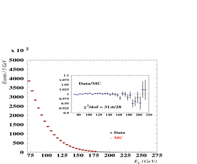
Figure 1: Comparison data–MC for the low kaon energy solution, the inset shows the ratio data/MC.

4.2 Monte–Carlo simulation

The detector response has been simulated in details using a MC program based on GEANT [15]. Particle interactions in the detector material as well as response functions of the different detector elements have been taken into account in the simulation. Pre–generated shower libraries for photons, electrons and charged pions are used to describe the response of the calorimeters.
To determine the detector acceptance as well as the distortion and losses of events on the Dalitz plot induced by the radiative effects, the $\rm K_{\mu 3}$ decay has been simulated both at the Born level and at the next–to–leading order (NLO). The acceptance suffers only from a residual dependence on the values (and on the type of parametrization) of the form factors used for the generation of the MC samples. To avoid any biases the samples were produced, after an iterative procedure, with values close to the results reported here. A linear parametrization was used with $\lambda_{+}^{gen}=0.0260$ and $\lambda_{0}^{gen}=0.0120$.
The NLO sample was obtained using as event generator KLOR [16], a program which numerically evaluates the radiative corrections and generates MC events. The simulated events underwent the same reconstruction procedure as the data events and the same selection cuts described in Sec 4.1 were applied. These two MC samples provide a statistics which is one order of magnitude larger than the data one.
A third, smaller, $\rm K_{\mu 3}$ sample was generated with full simulation of the showers in the calorimeters and was used to model the multiple scattering in the MUV. For detailed studies of the background samples of $\rm K_{e3}$, $\rm K_{3\pi}$ and $\rm K_{L}\rightarrow~{}\pi^{+}~{}\pi^{-}$ ($\rm K_{2\pi}$) decays decays were produced.
The $\rm K_{L}$ energy spectrum was extracted from the data by using the data distributions of the low and high energy solutions and the probability matrix, obtained from MC, which relates $E_{L}$ and $E_{H}$ to the true kaon energy.
To show the quality of the MC simulation the comparison of data and MC for some relevant kinematical quantities are shown in Fig. 1 to 3.

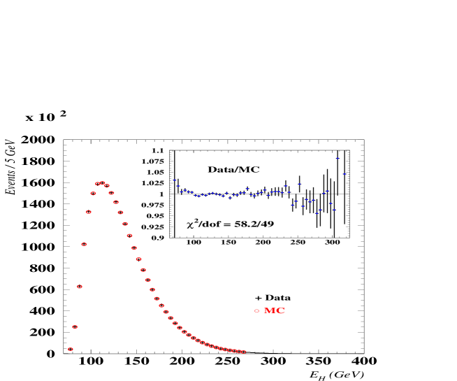
Figure 2: Comparison data–MC for the high kaon energy solution, the inset shows the ratio data/MC.

Figure 3: Comparison data–MC for the momentum distributions of muons, pions (lab system) and neutrinos (kaon CMS).

4.3 Backgrounds

The $\rm K_{e3}$, $\rm K_{3\pi}$ and $\rm K_{2\pi}$ decays are the major sources of background. A $\rm K_{e3}$ event can fake a genuine $\rm K_{\mu 3}$ when the $\pi$ decays into a muon and the $e$ has the $E/p$ requested for the identification of a $\pi~{}(E/p<0.9)$. To determine this source of contamination in the selected $\rm K_{\mu 3}$ sample, we used the $E/p$ distributions of tracks which pass all cuts, but not considering $E/p$. The electron signal is obtained by fitting this distribution around the value of 1. The integration of the fitted function into the ”pion” region allows to determine a value for the $\rm K_{e3}$ contamination of:

$$\mathcal{P}^{cont}_{Ke3}=(6.59\pm 0.09)\times 10^{-4}.$$ (8)

The $\rm K_{3\pi}$ decays (followed by the decay of one of the two charged $\pi$) are strongly suppressed by the $P_{0}^{{}^{\prime}2}$ cut. To determine the residual contamination the selected $\rm K_{\mu 3}$ events undergo a $\rm K_{3\pi}$ selection procedure: in the presence of clusters in the LKr not associated to the tracks, an attempt to reconstruct a $\pi^{0}$ is made. In case the two photons reconstruct the $\pi^{0}$ mass within a window of $\pm 6$ MeV/c², the invariant mass of the two tracks (assumed to be pions) and the $\pi^{0}$ is evaluated and if it falls in an interval of $\pm 9$ MeV/c² around the $K^{0}$ mass the event is assumed to be a $\rm K_{3\pi}$ decay. The number of these $\rm K_{3\pi}$ background events, corrected for their acceptance, allows to estimate for the $\rm K_{3\pi}$ contamination the value:

$$\mathcal{P}^{cont}_{3\pi}=(6.31\pm 0.16)\times 10^{-4}.$$ (9)

Another source of background stems from the $\rm K_{2\pi}$ decay with subsequent $\pi$ decay in flight or pion punch–through in the iron of the MUV. Using the $\rm K_{2\pi}$ MC sample this contamination is estimated to be:

$$\mathcal{P}^{cont}_{2\pi}=(5.63\pm 0.16)\times 10^{-4}.$$ (10)

This background source turns out to be the most dangerous one since the $\rm K_{2\pi}$ events populate a narrow region (the top right corner) of the $\rm K_{\mu 3}$ Dalitz plot introducing appreciable distortions. The $\rm K_{3\pi}$ events instead populate the bottom left region of the plot; being not much concentrated, they induce a smaller effect. Finally the $\rm K_{e3}$ events are distributed randomly on the plot and their effect is negligible.
Background events from $\rm K_{2\pi}$ and $\rm K_{3\pi}$ will be subtracted from the data while the effects of $\rm K_{e3}$ events will be included in the treatment of the systematic uncertainty related to the background (Sec.5.2).

5 Fitting procedure and results

5.1 Fitting procedure

The measurement reported here is based on the study of the Dalitz plot density.

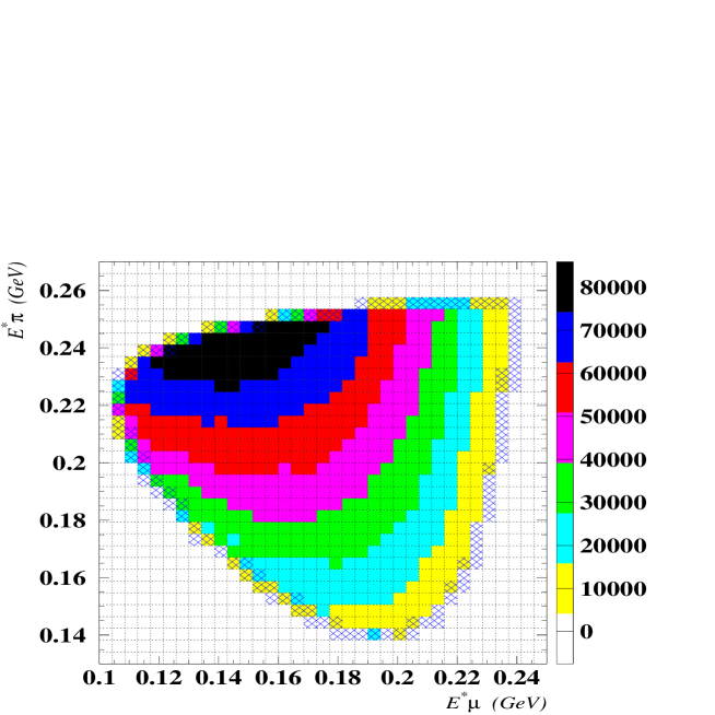
Figure 4: Dalitz plot distribution of the $\rm K_{\mu 3}$ events corrected for radiative effects and acceptance; the shaded cells are not used for the fit.

As mentioned before, the ambiguity in the determination of the kaon energy leads to two solutions for the $\rm K_{L}$ energy and for the CMS energies of the $\mu$ and the $\pi$. Consequently each event has a double location on the Dalitz plot. We chose to evaluate $E_{\mu}^{*}$ and $E_{\pi}^{*}$ by using only the low kaon energy solution. According to the MC simulation, this corresponds to the most probable solution, being in 61% of cases the correct one. The Dalitz plot was divided into cells with a dimension of about $4\times 4$ MeV² (see Fig. 4). About 39% of the events are reconstructed exactly in the same cell where they were generated, while this figure drops to 22% if the high solution is used. To extract the form factors we fit the data Dalitz plot, corrected for acceptance and radiative effects, to the Born level prediction. The acceptance, in the $i$–th cell of the plot, $\epsilon_{i}$, is defined as the ratio of the number of reconstructed events (evaluated using the low energy solution) to the number of generated events (evaluated using the true kaon energy) in that cell. We note that this definition of acceptance accounts also for the migration of events induced by the use of the low solution only.
The correction (for the $i$–th cell of the plot) due to the radiative effects is $(1+\delta)_{i}$ and is evaluated by taking the ratio between the number of reconstructed events from the MC–NLO sample and the number of reconstructed events from the MC–Born one.
The number of events, corrected for acceptance and radiative effects, in a given cell of the plot is therefore:

$$N_{i}=\frac{N_{i}^{Rec}}{\rule{0.0pt}{8.53581pt}\epsilon_{i}(1+\delta)_{i}},$$ (11)

where $N_{i}^{Rec}$ is the number of reconstructed and background subtracted data events.
The form factors were determined by fitting with the MINUIT [17] package the Dalitz plot distribution, corrected for acceptance and radiative effects, to the parametrization reported in Eq. 2. The cells crossed by the Dalitz plot boundary are excluded from the fit (see Fig. 4). Various $t$ dependences of the form factors were considered: linear, quadratic, pole and dispersive. The fit results are listed in Table 1; the correlations among the fitted form factors parameters are shown in Table 2. The comparison Data–Fit are shown in Fig. 5.

Linear ($\times 10^{-3}$)	$\lambda_{+}$	$\lambda_{0}$		$\chi^{2}$/ndf
	26.7$\pm$0.6	11.7$\pm$0.7		604.0/582
Quadratic ($\times 10^{-3}$)	$\lambda^{{}^{\prime}}_{+}$	$\lambda^{{}^{\prime\prime}}_{+}$	$\lambda_{0}$	$\chi^{2}$/ndf
	20.5$\pm$2.2	2.6$\pm$0.9	9.5$\pm$1.1	595.9/581
Pole (MeV/c2)	$m_{V}$	$m_{S}$		$\chi^{2}$/ndf
	905$\pm$9	1400$\pm$46		596.7/582
Dispersive ($\times 10^{-3}$)	$\Lambda_{+}$	$\ln C$		$\chi^{2}$/ndf
	23.3$\pm$0.5	143.8$\pm$8.0		595.0/582

Table 1: Form factors fit results for linear, quadratic pole and dispersive parametrizations. The quoted errors are the statistical ones.

We also fitted for a possible quadratic term in the scalar form factor and found $\lambda^{{}^{\prime\prime}}_{0}=(1.1\pm 1.3)\times 10^{-3}$ indicating that the linear assumption is sufficient to describe this form factor.

Linear		$\lambda_{0}$
	$\lambda_{+}$	-0.40
Quadratic		$\lambda^{{}^{\prime\prime}}_{+}$	$\lambda_{0}$
	$\lambda^{{}^{\prime}}_{+}$	-0.96	0.63
	$\lambda^{{}^{\prime\prime}}_{+}$	$-$	-0.73
Pole		$m_{S}$
	$m_{V}$	-0.47
Dispersive		$\Lambda_{+}$
	$\ln C$	-0.44

Table 2: Correlation coefficients among the fit parameters for the linear, quadratic, pole and dispersive parametrizations.

In the expansion of the vector form factor instead, evidence is present for the existence of both a linear and a quadratic term. We notice also a remarkable shift in the value of $\lambda_{0}$ as consequence of the presence of the quadratic term in the vector form factor expansion. The value of $m_{V}$ and $m_{S}$, obtained with the pole fit are found to be consistent with the $\rm K^{*}(892)$ and $\rm K^{*}(1430)$ masses, respectively.

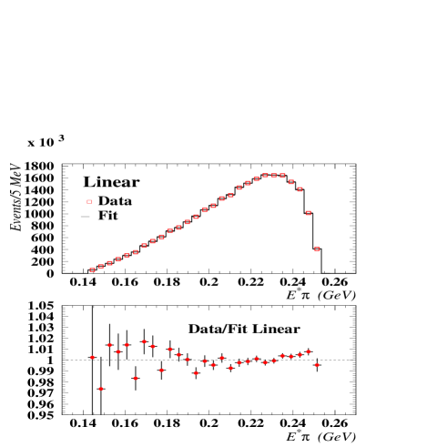
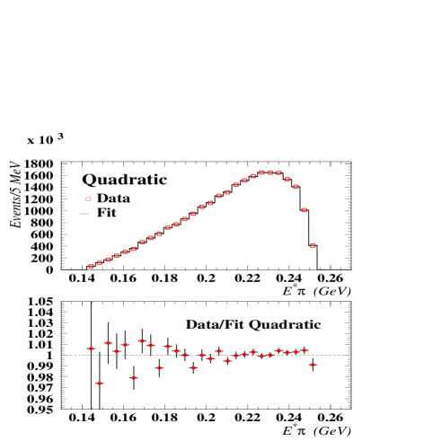
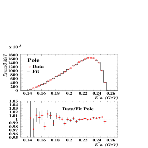
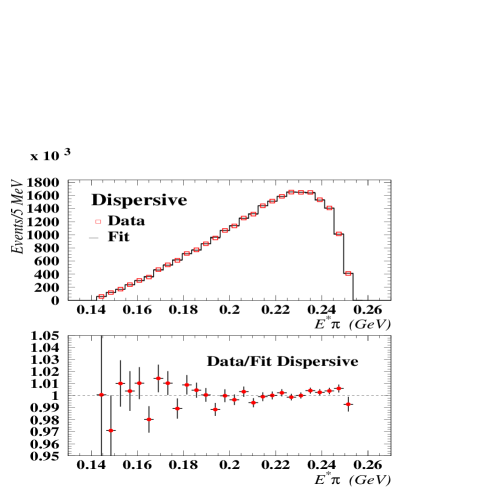
Figure 5: Comparison Data–Fits and Data/Fit ratios for the four parametrization used in the analysis. For visualization purposes the various Dalitz plots distributions have been projected onto the $E_{\pi}^{*}$ axis.

As a cross–check we extracted the linear form factors using a $\chi^{2}$ built by comparing the data Dalitz plot distribution, corrected for radiative effects only, with a set of Born level plots of reconstructed MC events. Each MC Dalitz plot distribution was produced with different form factors values by proper re–weighting of the events of the reference MC–Born sample. The form factors values are extracted by minimizing the $\chi^{2}(\lambda_{+},~{}\lambda_{0})$ function constructed in this way. The results obtained with this method are less accurate than those provided by the fit procedure but fully unbiased with respect to the choice of the form factors values used to generate the MC sample. These results are in perfect agreement with the ones obtained with the fit procedure, indicating the absence of such kind of bias in the analysis procedure.
To check the fit procedure we fitted MC events, using the reference MC sample (generated with linear parametrization) and smaller samples generated with quadratic and pole parametrizations. In all the three cases the input form factors were correctly reproduced at the end of the process, indicating the absence of any bias in the fit procedure.

5.2 Systematic uncertainties

Various sources of systematic uncertainties in the determination of the form factors have been investigated. Their individual contributions are reported on Table 3 together with the effects related to the background contamination. The total error was obtained by combining the individual errors in quadrature.

	$\Delta$$\lambda_{+}$	$\Delta$$\lambda_{0}$	$\Delta\lambda_{+}^{{}^{\prime}}$	$\Delta\lambda_{+}^{{}^{\prime\prime}}$	$\Delta$$\lambda_{0}$	$\Delta m_{V}$	$\Delta m_{S}$	$\Delta\Lambda_{+}$	$\Delta\ln C$
	$\times 10^{-3}$					MeV/c2		$\times 10^{-3}$
Background	$\pm$0.0	$\pm$0.1	$\pm$0.2	$\pm$0.1	$\pm$0.0	$\pm$0	$\pm$5	$\pm$0.0	$\pm$1.2
Acceptance	$\pm$0.4	$\pm$0.5	$\pm$0.7	$\pm$0.4	$\pm$0.4	$\pm$7	$\pm$22	$\pm$0.4	$\pm$5.0
$TRK_{dist}$ @ LKr	$\pm$0.4	$\pm$0.4	$\pm$0.5	$\pm$0.4	$\pm$0.3	$\pm$10	$\pm$20	$\pm$0.4	$\pm$5.4
$P_{MIN}$	$\pm$0.1	$\pm$0.3	$\pm$0.4	$\pm$0.1	$\pm$0.3	$\pm$1	$\pm$20	$\pm$0.1	$\pm$3.1
$P_{\nu}^{*}-P_{\nu T}$	$\pm$0.2	$\pm$0.2	$\pm$0.5	$\pm$0.2	$\pm$0.2	$\pm$6	$\pm$10	$\pm$0.2	$\pm$2.2
$\rm K_{L}$  spectrum	$\pm$0.2	$\pm$0.4	$\pm$0.0	$\pm$0.0	$\pm$0.3	$\pm$4	$\pm$20	$\pm$0.2	$\pm$4.1
HIGH solution	$\pm$0.3	$\pm$0.0	$\pm$0.6	$\pm$0.2	$\pm$0.2	$\pm$8	$\pm$12	$\pm$0.4	$\pm$1.9
MUV reconstruction	$\pm$0.1	$\pm$0.1	$\pm$0.1	$\pm$0.0	$\pm$0.1	$\pm$2	$\pm$5	$\pm$0.2	$\pm$0.8
Radiative corrections	$\pm$0.2	$\pm$0.4	$\pm$2.0	$\pm$0.7	$\pm$0.3	$\pm$2	$\pm$20	$\pm$0.1	$\pm$4.3
Cell Size	$\pm$0.3	$\pm$0.3	$\pm$0.5	$\pm$0.3	$\pm$0.3	$\pm$5	$\pm$20	$\pm$0.2	$\pm$4.0
Total Systematic	$\pm$0.8	$\pm$1.0	$\pm$2.4	$\pm$1.0	$\pm$0.8	$\pm$17	$\pm$53	$\pm$0.8	$\pm$11.2
Statistical	$\pm$0.6	$\pm$0.7	$\pm$2.2	$\pm$0.9	$\pm$1.1	$\pm$9	$\pm$46	$\pm$0.5	$\pm$8.0
Total Error	$\pm$1.0	$\pm$1.2	$\pm$3.3	$\pm$1.3	$\pm$1.4	$\pm$19	$\pm$70	$\pm$0.9	$\pm$13.8

Table 3: Systematic and total uncertainties for the four form factor parametrizations analyzed. The systematic and statistical uncertainties have been added in quadrature to obtain the total error.

Effects related to the background have been checked altering the estimated contaminations by 15% and accounting for the tiny effect related to $\rm K_{e3}$ events. The variations in the fit results were taken as the systematic uncertainty.
Effects related to the acceptance and selection criteria have been checked by varying the selection cuts in a reasonable range. The largest fluctuations in the form factors were taken as systematic errors.
Effects related to the $\rm K_{L}$  energy spectrum used in the MC simulations were investigated by using the spectrum obtained from a clean sample of $\rm K_{2\pi}$ decays. The simulated events were re–weighted with the ratio of the two spectra, and the differences in the form factor results were taken as the systematic uncertainty.
To check effects related to the use of the low kaon energy solution the analysis was repeated using the high solution to determine the acceptance and radiative corrections. Also in this case the differences with the reference fit results were taken as systematic error.
The inefficiency of the MUV during this run was measured by identifying the $\mu$ according to its energy deposition in the electromagnetic and hadronic (HAC) calorimeters. The MUV efficiency was found to vary between 0.97 for a 10 GeV/c and 1 for a $\geq 20$ GeV/c muon with an average of $\epsilon_{MUV}=0.9987\pm 0.0001$. To investigate possible biases, the inefficiency was artificially increased by randomly rejecting events according to the momentum dependence of the efficiency and its value, without observing any significant effect.
Effects related to the MUV offline reconstruction were tested by relaxing the cut between the track extrapolation and the hit position and by accepting also events for which only plane 1 and 2, but not plane 3, had fired. This produces an increase of 3.2% in the statistics of the data sample; here again differences from the reference form factor values were taken as systematic error.
Effects related to the radiative corrections model used in the analysis were tested by applying the corrections obtained with the Ginsberg [18] formalism, amending the error reported in Ref. [19] and allowing for a $t$ dependence of the form factors. The differences with the reference results were taken as an estimate of the systematic effect.
The effects related to the size of the cells in which the Dalitz plot was divided were determind by reducing the cell size down to about $3\times 3$ MeV², the largest fluctuations in the form factors were taken as systematic errors.
To estimate the possible influence of accidental particles, tracks outside the allowed time window for a match in the MUV were studied. No effect was found from this source.

6 Conclusions

The $\rm K_{\mu 3}$ decay has been studied with the NA48 detector. A sample of 2.3$\times 10^{6}$ reconstructed events was analyzed in order to extract the decay form factors. Studying the Dalitz plot density we measured the following values for the form factors parameters: $\lambda^{{}^{\prime}}_{+}=(20.5\pm 2.2_{stat}\pm 2.4_{syst})\times 10^{-3}$, $\lambda^{{}^{\prime\prime}}_{+}=(2.6\pm 0.9_{stat}\pm 1.0_{syst})\times 10^{-3}$ and $\lambda_{0}=(9.5\pm 1.1_{stat}\pm 0.8_{syst})\times 10^{-3}$.
Our results indicate the presence of a quadratic term in the expansion of the vector form factor in agreement with other recent analyses of kaon semileptonic decays. Fig. 6 shows the comparison between the results of the quadratic fits as reported by the recent experiments [11, 9, 10, 7, 8]. The 1 $\sigma$ contour plots are shown, both for $\rm K_{e3}$ and $\rm K_{\mu 3}$ decays; the ISTRA+ results have been multiplied by the ratio $(m_{\pi^{+}}/m_{\pi^{0}})^{2}$. The results are higly correlated, those from this measurement and from KTeV have a larger quadratic term and appear only in partial agreement with the other $\rm K_{e3}$ experiments. We notice however that the observed spread in the $\lambda^{{}^{\prime}}_{+}$, $\lambda^{{}^{\prime\prime}}_{+}$ figures is greatly reduced if the values obtained from the Taylor expansion of the pole parametrization ($\lambda^{{}^{\prime}}_{+}=m_{\pi}^{2}/m_{V}^{2}$; $\lambda^{{}^{\prime\prime}}_{+}=2\lambda^{{}^{\prime}2}_{+}$) are used.
Using a linear fit our results were: $\lambda_{+}=(26.7\pm 0.6_{stat}\pm 0.8_{syst})\times 10^{-3}$ and, $\lambda_{0}=(11.7\pm 0.7_{stat}\pm 1.0_{syst})\times 10^{-3}$. While the result for $\lambda_{+}$  is well compatible with the recent (and most precise) KTeV measurement, the value of $\lambda_{0}$ appears to be shifted towards lower values. A pole fit of the form factors yields: $m_{V}=(905\pm 9_{stat}\pm 17_{syst})$ MeV/c² and $m_{S}=(1400\pm 46_{stat}\pm 53_{syst})$ MeV/c² in agreement with the $\rm K^{*}(892)$ and $\rm K^{*}(1430)$ masses, respectively. In Fig. 7 is shown a comparison between our results and those of [9] and [11] for this parametrization.
Using the recently proposed parametrization based on a dispersive approach, we obtain for the slope of the vector form factor: $\Lambda_{+}=(23.3\pm 0.5_{stat}\pm 0.8_{syst})\times 10^{-3}$ and for the logarithm of the scalar form factor at the Callan–Treiman point: $\ln C=(143.8\pm 8.0_{stat}\pm 11.2_{syst})\times 10^{-3}$. According to the model proposed in [4] the value of $\ln C$ can be used to test the existence of RHCs by comparing it with the Standard Model predictions. Taking the value of $|F_{K+}V_{us}/F_{\pi+}V_{ud}|$ from [20] and those of $f_{+}(0)|V_{us}|$ and $|V_{ud}|$ from [21] we obtain for a combination of the RHCs couplings and the Callan–Treiman discrepancy ($\tilde{\Delta}_{CT}$) the value: $2(\epsilon_{S}-\epsilon_{NS})+\tilde{\Delta}_{CT}=-0.071\pm 0.014_{NA48}\pm 0.002_{theo}\pm 0.005_{ext}$, where the first error is the combination in quadrature of the statistical and systematical uncertainties, the second one refers to the uncertainties related to the approximations used to replace the dispersion integrals and the last one is due to the external experimental input.

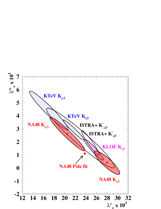
Figure 6: 1 $\sigma$ contour plots in the plane $\lambda^{{}^{\prime}}_{+}$–$\lambda^{{}^{\prime\prime}}_{+}$ showing the NA48 results together with those of [9, 7, 11] for the quadratic fits of the $\rm K_{\mu 3}$ and $\rm K_{e3}$ decays. The dot represents $\lambda^{{}^{\prime}}_{+}$ and $\lambda^{{}^{\prime\prime}}_{+}$ as obtained with a Taylor expansion of the pole parametrization. The ISTRA+ results have been multiplied by the ratio $(m_{\pi^{+}}/m_{\pi^{0}})^{2}$.

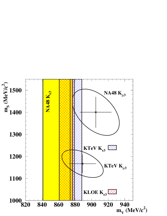
Figure 7: NA48 pole fits results, together with those of [9] and [11], for $\rm K_{\mu 3}$ and $\rm K_{e3}$ decays. $\rm K_{e3}$ results appear as vertical bands on the $m_{V}$–$m_{S}$ plane; the ellipses shown for $\rm K_{\mu 3}$ results are the 68% C.L. contour plots.

References

- [1] L.-M. Chounet, J.-M. Gaillard, M.K. Gaillard, Phys. Rep. 4C, (1972) 199.
- [2] H. Leutwyler, M. Roos, Z. Phys. C 25, (1984) 91.
- [3] J. Bijnens, P. Talavera, Nucl. Phys. B 669, (2003) 341.
- [4] V. Bernard, M. Oertel, E. Passmar and J. Stern, Phys. Lett. B 638, (2006) 480.
- [5] R. F. Dashen and M. Weinstein, Phys. Rev. Lett. 22, (1969) 1337.
- [6] S. Eidelman et al., Phys. Lett. B 592, (2004) 1.
- [7] O.P. Yushchenko et al. (ISTRA+ Coll.), Phys. Lett. B 589, (2004) 111.
- [8] O.P. Yushchenko et al. (ISTRA+ Coll.), Phys. Lett. B 581, (2004) 31.
- [9] T. Alexopoulos et al. (KTeV Coll.), Phys. Rev. D 70, (2004) 092007.
- [10] A. Lai et al. (NA48 Coll.), Phys. Lett. B 604, (2004) 1.
- [11] F. Ambrosino et al. (KLOE Coll.), Phys. Lett. B 636, (2006) 166.
- [12] P. Lichard, Phys. Rev. D 55, (1997) 5385.
- [13] J. Stern, private communication.
- [14] A. Lai et al. (NA48 Coll.), Eur. Phys. J. C 22, (2001) 231.
- [15] CERN Program Library Long Writeup, W5013 (1993).
- [16] T. Andre, hep-ph/0406006 and Nucl. Phys. B Proc. Suppl. 142, (2005) 58.
- [17] F. James, CERN Program Library Long Writeup, D506 (1998).
- [18] E. Ginsberg, Phys. Rev. D 1, (1970) 229.
- [19] V. Cirigliano et al., Eur. Phys. J. C 23, (2002) 121.
- [20] M. Jamin, J. A. Oller and A. Pich, Phys. Rev. D 74, (2006) 074009.
- [21] W.–M Yao et al., Journ. Phys. G. 33, (2006) 1.