Daya Bay

Proposal

December 1, 2006

A Precision Measurement of the Neutrino Mixing Angle $\theta_{13}$ Using Reactor Antineutrinos At Daya Bay

Daya Bay Collaboration

Beijing Normal University

Xinheng Guo, Naiyan Wang, Rong Wang

Brookhaven National Laboratory

Mary Bishai, Milind Diwan, Jim Frank, Richard L. Hahn, Kelvin Li, Laurence Littenberg, David Jaffe, Steve Kettell, Nathaniel Tagg, Brett Viren, Yuping Williamson, Minfang Yeh

California Institute of Technology

Christopher Jillings, Jianglai Liu, Christopher Mauger, Robert McKeown

Charles Unviersity

Zdenek Dolezal, Rupert Leitner, Viktor Pec, Vit Vorobel

Chengdu University of Technology

Liangquan Ge, Haijing Jiang, Wanchang Lai, Yanchang Lin

China Institute of Atomic Energy

Long Hou, Xichao Ruan, Zhaohui Wang, Biao Xin, Zuying Zhou

Chinese University of Hong Kong,

Ming-Chung Chu, Joseph Hor, Kin Keung Kwan, Antony Luk

Illinois Institute of Technology

Christopher White

Institute of High Energy Physics

Jun Cao, Hesheng Chen, Mingjun Chen, Jinyu Fu, Mengyun Guan, Jin Li, Xiaonan Li, Jinchang Liu, Haoqi Lu, Yusheng Lu, Xinhua Ma, Yuqian Ma, Xiangchen Meng, Huayi Sheng, Yaxuan Sun, Ruiguang Wang, Yifang Wang, Zheng Wang, Zhimin Wang, Liangjian Wen, Zhizhong Xing, Changgen Yang, Zhiguo Yao, Liang Zhan, Jiawen Zhang, Zhiyong Zhang, Yubing Zhao, Weili Zhong, Kejun Zhu, Honglin Zhuang

Iowa State University

Kerry Whisnant, Bing-Lin Young

Joint Institute for Nuclear Research

Yuri A. Gornushkin, Dmitri Naumov, Igor Nemchenok, Alexander Olshevski

Kurchatov Institute

Vladimir N. Vyrodov

Lawrence Berkeley National Laboratory and University of California at Berkeley

Bill Edwards, Kelly Jordan, Dawei Liu, Kam-Biu Luk, Craig Tull

Nanjing University

Shenjian Chen, Tingyang Chen, Guobin Gong, Ming Qi

Nankai University

Shengpeng Jiang, Xuqian Li, Ye Xu

National Chiao-Tung University

Feng-Shiuh Lee, Guey-Lin Lin, Yung-Shun Yeh

National Taiwan University

Yee B. Hsiung

National United University

Chung-Hsiang Wang

Princeton University

Changguo Lu, Kirk T. McDonald

Rensselaer Polytechnic Institute

John Cummings, Johnny Goett, Jim Napolitano, Paul Stoler

Shenzhen Univeristy

Yu Chen, Hanben Niu, Lihong Niu

Sun Yat-Sen (Zhongshan) University

Zhibing Li

Tsinghua University

Shaomin Chen, Hui Gong, Guanghua Gong, Li Liang, Beibei Shao, Qiong Su, Tao Xue, Ming Zhong

University of California at Los Angeles

Vahe Ghazikhanian, Huan Z. Huang, Charles A. Whitten, Stephan Trentalange

University of Hong Kong,

K.S. Cheng, Talent T.N. Kwok, Maggie K.P. Lee, John K.C. Leung, Jason C.S. Pun, Raymond H.M. Tsang, Heymans H.C. Wong

University of Houston

Michael Ispiryan, Kwong Lau, Logan Lebanowski, Bill Mayes, Lawrence Pinsky, Guanghua Xu

University of Illinois at Urbana-Champaign

S. Ryland Ely, Wah-Kai Ngai, Jen-Chieh Peng

University of Science and Technology of China

Qi An, Yi Jiang, Hao Liang, Shubin Liu, Wengan Ma, Xiaolian Wang, Jian Wu, Ziping Zhang, Yongzhao Zhou

University of Wisconsin

A. Baha Balantekin, Karsten M. Heeger, Thomas S. Wise

Virginia Polytechnic Institute and State University

Jonathan Link, Leo Piilonen

Preprint numbers:
BNL-77369-2006-IR
LBNL-62137
TUHEP-EX-06-003

Executive Summary

This document describes the design of the Daya Bay reactor neutrino experiment. Recent discoveries in neutrino physics have shown that the Standard Model of particle physics is incomplete. The observation of neutrino oscillations has unequivocally demonstrated that the masses of neutrinos are nonzero. The smallness of the neutrino masses ($<$2 eV) and the two surprisingly large mixing angles measured have thus far provided important clues and constraints to extensions of the Standard Model.

The third mixing angle, $\theta_{13}$, is small and has not yet been determined; the current experimental bound is $\sin^{2}2\theta_{13}<$ 0.17 at 90% confidence level (from Chooz) for $\Delta m^{2}_{31}=2.5\times 10^{-3}$ eV². It is important to measure this angle to provide further insight on how to extend the Standard Model. A precision measurement of $\sin^{2}2\theta_{13}$ using nuclear reactors has been recommended by the 2004 APS Multi-divisional Study on the Future of Neutrino Physics as well as a recent Neutrino Scientific Assessment Group (NuSAG) report.

We propose to perform a precision measurement of this mixing angle by searching for the disappearance of electron antineutrinos from the nuclear reactor complex in Daya Bay, China. A reactor-based determination of $\sin^{2}2\theta_{13}$ will be vital in resolving the neutrino-mass hierarchy and future measurements of $CP$ violation in the lepton sector because this technique cleanly separates $\theta_{13}$ from $CP$ violation and effects of neutrino propagation in the earth. A reactor-based determination of $\sin^{2}2\theta_{13}$ will provide important, complementary information to that from long-baseline, accelerator-based experiments. The goal of the Daya Bay experiment is to reach a sensitivity of 0.01 or better in $\sin^{2}2\theta_{13}$ at 90% confidence level.

The Daya Bay Experiment

The Day Bay nuclear power complex is one of the most prolific sources of antineutrinos in the world. Currently with two pairs of reactor cores (Daya Bay and Ling Ao), separated by about 1.1 km, the complex generates 11.6 GW of thermal power; this will increase to 17.4 GW by early 2011 when a third pair of reactor cores (Ling Ao II) is put into operation and Daya Bay will be among the five most powerful reactor complexes in the world. The site is located adjacent to mountainous terrain, ideal for siting underground detector laboratories that are well shielded from cosmogenic backgrounds. This site offers an exceptional opportunity for a reactor neutrino experiment optimized to perform a precision determination of $\sin^{2}2\theta_{13}$ through a measurement of the relative rates and energy spectrum of reactor antineutrinos at different baselines. In addition, this project offers a unique and unprecedented opportunity for scientific collaboration involving China, the U.S., and other countries.

The basic experimental layout of Daya Bay consists of three underground experimental halls, one far and two near, linked by horizontal tunnels. Figure 0.1 shows the detector module deployment at these sites.

Figure 0.1: Default configuration of the Daya Bay experiment, optimized for best sensitivity in sin${}^{2}2\theta_{13}$. Four detector modules are deployed at the far site and two each at each of the near sites.

Eight identical cylindrical detectors, each consisting of three nested cylindrical zones contained within a stainless steel tank, will be deployed to detect antineutrinos via the inverse beta-decay reaction. To maximize the experimental sensitivity four detectors are deployed in the far hall at the first oscillation maximum. The rate and energy distribution of the antineutrinos from the reactors are monitored with two detectors in each near hall at relatively short baselines from their respective reactor cores, reducing the systematic uncertainty in $\sin^{2}2\theta_{13}$ due to uncertainties in the reactor power levels to about 0.1%. This configuration significantly improves the statistical precision over previous experiments (0.2% in three years of running) and enables cross-calibration to verify that the detectors are identical. Each detector will have 20 metric tons of 0.1% Gd-doped liquid scintillator in the inner-most, antineutrino target zone. A second zone, separated from the target and outer buffer zones by transparent acrylic vessels, will be filled with undoped liquid scintillator for capturing gamma rays that escape from the target thereby improving the antineutrino detection efficiency. A total of 224 photomultiplier tubes are arranged along the circumference of the stainless steel tank in the outer-most zone, which contains mineral oil to attenuate gamma rays from trace radioactivity in the photomultiplier tube glass and nearby materials including the outer tank. The detector dimensions are summarized in Table 0.1.

Dimensions	Inner Acrylic	Outer Acrylic	Stainless Steel
Diameter (mm)	3200	4100	5000
Height (mm)	3200	4100	5000
Wall thickness (mm)	10	15	10
Vessel Weight (ton)	0.6	1.4	20
Liquid Weight (ton)	$\sim$20	$\sim$20	$\sim$40

Table 0.1: Summary of antineutrino detector properties. The liquid weights are for the mass of liquid contained only within that zone.

With reflective surfaces at the top and bottom of the detector the energy resolution of the detector is about 12% at 1 MeV.

The mountainous terrain provides sufficient overburden to suppress cosmic muon induced backgrounds to less than 1% of the antineutrino signal. The detectors in each experimental hall are shielded by 2.5 m of water from radioactivity and spallation neutrons in the surrounding rock. The detector halls include a muon detector system, consisting of a tracker on top of the water pool and water Cherenkov counters in the water shield, for tagging the residual cosmic muons.

With this experimental setup, the signal and background rates at the Daya Bay near hall, Ling Ao near hall and the far hall are summarized in Table 0.2.

	Daya Bay Near	Ling Ao Near	Far Hall
Baseline (m)	363	481 from Ling Ao	1985 from Daya Bay
		526 from Ling Ao II	1615 from Ling Ao’s
Overburden (m)	98	112	350
Radioactivity (Hz)	$<$50	$<$50	$<$50
Muon rate (Hz)	36	22	1.2
Antineutrino Signal (events/day)	930	760	90
Accidental Background/Signal (%)	$<$0.2	$<$0.2	$<$0.1
Fast neutron Background/Signal (%)	0.1	0.1	0.1
8He+9Li Background/Signal (%)	0.3	0.2	0.2

Table 0.2: Summary of signal and background rates for each detector module at the different experimental sites.

Careful construction, filling, calibration and monitoring of the detectors will reduce detector-related systematic uncertainties to a level comparable to or below the statistical uncertainty. Table 0.3 is a summary of systematic uncertainties for the experiment.

Source	Uncertainty
Reactor Power	0.087% (4 cores)
	0.13% (6 cores)
Detector (per module)	0.38% (baseline)
	0.18% (goal)
Signal Statistics	0.2%

Table 0.3: Summary of uncertainties. The baseline value is realized through proven experimental methods, whereas the goal value should be attainable with additional research and development.

The horizontal tunnels connecting the detector halls will facilitate cross-calibration and offer the possibility of swapping the detectors to further reduce systematic uncertainties.

Civil construction is scheduled to begin in the spring of 2007. Deployment of the first pair of the detectors in one of the near halls will start in February 2009. Data taking using the baseline configuration of two near halls and the far hall will begin in June 2010. With three years of running and the estimated signal and background rates as well as systematic uncertainties, the sensitivity of Daya Bay for $\sin^{2}2\theta_{13}$ is 0.008 or better, relatively independent of the value of $\Delta m^{2}_{31}$ within its currently allowed range.

Contents

1. Executive Summary
2. 1 Physics
   1. 1.1 Neutrino Oscillations
   2. 1.2 Neutrino Mixing
      1. 1.2.1 Current Knowledge of Mixing Parameters
   3. 1.3 Significance of the Mixing Angle $\theta_{13}$
      1. 1.3.1 Impact on the experimental program
      2. 1.3.2 Impact on theoretical development
   4. 1.4 Complementarity of Reactor-based and Accelerator-based Neutrino Oscillation Experiments
   5. 1.5 Reactor Antineutrino Experiments
      1. 1.5.1 Energy Spectrum and Flux of Reactor Antineutrinos
      2. 1.5.2 Inverse Beta-Decay Reaction
      3. 1.5.3 Observed Antineutrino Rate and Spectrum at Short Distance
      4. 1.5.4 Reactor Antineutrino Disappearance Experiments
   6. 1.6 Determining $\theta_{13}$ with Nuclear Reactors
      1. 1.6.1 Past Measurements
      2. 1.6.2 Precision Measurement of $\theta_{13}$
   7. 1.7 The Daya Bay Reactor Antineutrino Experiment
3. 2 Experimental Design Overview
   1. 2.1 Experimental layout
   2. 2.2 Detector Design
      1. 2.2.1 Antineutrino detector
      2. 2.2.2 Muon detector
   3. 2.3 Alternative Designs of the Water Buffer
4. 3 Sensitivity & Systematic Uncertainties
   1. 3.1 Reactor Related Uncertainties
      1. 3.1.1 Power Fluctuations
      2. 3.1.2 Location Uncertainties
      3. 3.1.3 Spent Fuel Uncertainties
   2. 3.2 Detector Related Uncertainties
      1. 3.2.1 Target Mass and H/C Ratio
      2. 3.2.2 Position Cuts
      3. 3.2.3 Positron Energy Cut
      4. 3.2.4 Neutron Detection Efficiency
      5. 3.2.5 Neutron Multiplicity
      6. 3.2.6 Trigger
      7. 3.2.7 Live Time
   3. 3.3 Cross-calibration and Swapping of Detectors
      1. 3.3.1 Detector Swapping
      2. 3.3.2 Detector Cross-calibration
   4. 3.4 Backgrounds
      1. 3.4.1 Cosmic Muons in the Underground Laboratories
      2. 3.4.2 Simulation of Neutron Backgrounds
      3. 3.4.3 Cosmogenic Isotopes
      4. 3.4.4 Radioactivity
      5. 3.4.5 Background Subtraction Uncertainty
   5. 3.5 Sensitivity
      1. 3.5.1 Global $\chi^{2}$ Analysis
      2. 3.5.2 $\theta_{13}$ Sensitivity
5. 4 Experimental Site and Laboratories
   1. 4.1 General Laboratory Facilities
      1. 4.1.1 Tunnels
   2. 4.2 Site Survey
      1. 4.2.1 Topographic Survey
      2. 4.2.2 Engineering Geological Mapping
      3. 4.2.3 Geophysical Exploration
      4. 4.2.4 Engineering Drilling
      5. 4.2.5 On-site Test at Boreholes
      6. 4.2.6 Laboratory Tests
      7. 4.2.7 Survey Summary
   3. 4.3 Conceptual Design
      1. 4.3.1 Transportation Vehicle for the Antineutrino Detectors
      2. 4.3.2 Lifting System for the Antineutrino Detectors
      3. 4.3.3 Experimental Hall Layout
      4. 4.3.4 Design of Tunnel
      5. 4.3.5 Other Facilities
   4. 4.4 Civil Construction Overview
6. 5 Antineutrino Detectors
   1. 5.1 Overview
      1. 5.1.1 Module Geometry
      2. 5.1.2 Target Mass
      3. 5.1.3 Three-zone Antineutrino Detector
      4. 5.1.4 $\gamma$-Catcher
      5. 5.1.5 Oil Buffer
      6. 5.1.6 2-zone vs. 3-zone Detector
      7. 5.1.7 Expected Performance
   2. 5.2 Containers and Calibration Ports
      1. 5.2.1 Acrylic Vessel
      2. 5.2.2 Calibration Ports
   3. 5.3 Liquid Scintillator
      1. 5.3.1 Selection of Solvents
      2. 5.3.2 Preparation of Gadolinium Complexes
      3. 5.3.3 Purification of Individual Components for Gd-LS
      4. 5.3.4 Characterization of Gd-LS
      5. 5.3.5 Comparisons with Commercial Gd-LS
      6. 5.3.6 Large Scale Production of Gd-LS
      7. 5.3.7 Storing and Handling of LS at Daya Bay
   4. 5.4 Antineutrino Detector Photomultiplier Tubes
      1. 5.4.1 PMT Selection Options
      2. 5.4.2 PMT Testing
      3. 5.4.3 PMT Support Structure
      4. 5.4.4 High-Voltage System
   5. 5.5 Front End Electronics
      1. 5.5.1 Front-End Electronics Specifications
      2. 5.5.2 Front End Boards
   6. 5.6 Antineutrino Detector Prototype
      1. 5.6.1 Prototype Detector Design
      2. 5.6.2 Prototype Detector Test Results
7. 6 Calibration and Monitoring Systems
   1. 6.1 Radioactive Sources
   2. 6.2 LED Calibration System
   3. 6.3 In-situ Detector Monitoring
   4. 6.4 Detector monitoring with data
   5. 6.5 Automated Deployment System
   6. 6.6 Manual deployment system
8. 7 Muon System
   1. 7.1 Muon System Specifications
      1. 7.1.1 Muon Detection Efficiency
      2. 7.1.2 Muon System Redundancy
      3. 7.1.3 Spatial Resolution
      4. 7.1.4 Timing Resolution
      5. 7.1.5 Water Shield Thickness
      6. 7.1.6 Summary of Requirements
   2. 7.2 Water Buffer
      1. 7.2.1 Water Buffer Design
      2. 7.2.2 Water Shield PMT layout
      3. 7.2.3 Water Shield Simulation Studies
      4. 7.2.4 Water Buffer Front-End Electronics
      5. 7.2.5 Calibration of the Water Buffer PMTs
      6. 7.2.6 Purification of the Water Buffer
   3. 7.3 Muon Tracker
      1. 7.3.1 Resistive Plate Chambers (RPC)
      2. 7.3.2 RPC Design
      3. 7.3.3 RPC Mounting
      4. 7.3.4 RPC Performance
      5. 7.3.5 RPC Front-End Electronics
      6. 7.3.6 Water Cherenkov Modules
      7. 7.3.7 Plastic Scintillator Strips
      8. 7.3.8 Scintillator Strip Performance
      9. 7.3.9 Scintillator Strip Front-End Electronics
9. 8 Trigger and Data Acquisition System
   1. 8.1 The Trigger System
      1. 8.1.1 Requirements
      2. 8.1.2 The Antineutrino Detector Trigger System
      3. 8.1.3 The Muon Trigger System
   2. 8.2 The Timing System
      1. 8.2.1 Timing Master Clock
      2. 8.2.2 Timing Control Board
      3. 8.2.3 Timing Signal Fanout
   3. 8.3 The Data Acquisition System
      1. 8.3.1 Requirements
      2. 8.3.2 The DAQ System Architecture
   4. 8.4 Detector Control and Monitoring
10. 9 Installation, System Testing, and Detector Deployment
    1. 9.1 Receiving and Storage of Detector Components
    2. 9.2 Surface Assembly Building
    3. 9.3 Assembly of the Antineutrino Detectors
    4. 9.4 Precision Survey of Detector Modules
    5. 9.5 Subsystem Testing
    6. 9.6 Filling the Detector Modules
    7. 9.7 Transport to Experimental Halls
    8. 9.8 Final Integration in the Experimental Halls
    9. 9.9 Early Occupancy of the Experimental Halls at the Near and Mid Sites
    10. 9.10 Precision Placement and Alignment
11. 10 Operations of the Daya Bay Experiment
    1. 10.1 Configurations of Detector Modules
    2. 10.2 Detector Swapping
    3. 10.3 Logistics of Detector Swapping
12. 11 Schedule and Scope
    1. 11.1 Project Schedule
    2. 11.2 Project Scope
13. A Acknowledgements
14. B Acronyms

List of Figures

1. 0.1 Default configuration of the Daya Bay experiment, optimized for best sensitivity in sin${}^{2}2\theta_{13}$. Four detector modules are deployed at the far site and two each at each of the near sites.
2. 1.1 Global fits to $\sin^{2}\theta_{13}$.
3. 1.2 Resolving ambiguity in $\theta_{23}$ with $\sin^{2}2\theta_{13}$ determined by reactor experiments. Not only does the reactor experiment provide a precise measurement of $\sin^{2}2\theta_{13}$, but it provides a precise measurement of $\theta_{23}$ by resolving an ambiguity in the interpretation of the accelerator data.
4. 1.3 Fission rate of reactor isotopes as a function of time.
5. 1.5.1 Energy Spectrum and Flux of Reactor Antineutrinos
6. 1.6 Total cross section for inverse beta-decay calculated in leading order and next-to-leading order.
7. 1.5.2 Inverse Beta-Decay Reaction
8. 1.9 Antineutrino energy spectrum, total inverse beta-decay cross section, and count rate as a function of antineutrino energy.
9. 1.10 Reactor antineutrino disappearance probability as a function of distance from the source.
10. 1.11 Reactor antineutrino disappearance probability due to the mixing angle $\theta_{13}$ as a function of the baseline $L_{\rm far}$ over the allowed 2$\sigma$ range in $\Delta{m}^{2}_{32}$.
11. 1.12 Exclusion contours determined by Chooz, Palo Verde along with the allowed region obtained by Kamiokande.
12. 1.13 Daya Bay and vicinity: The nuclear power complex is located about 55 km from central Hong Kong.
13. 1.14 The Daya Bay nuclear power complex. The Daya Bay nuclear power plant is in the foreground. The Ling Ao nuclear power plant is in the background. The experimental halls will be underneath the hills to the left.
14. 2.1 Layout of the Daya Bay experiment.
15. 2.2 Site optimization using the global $\chi^{2}$ analysis. The optimal sites are labelled with red triangles. The stars show the reactors. The black contours show the sensitivity when one site’s location is varied and the other two are fixed at optimal sites. The red lines with tick marks are the perpendicular bisectors of the reactor pairs. The mountain contours are also shown on the plot (blue lines).
16. 2.3 Layout of the baseline design of the Daya Bay detector. Four antineutrino detector modules are shielded by a 1.5 m-thick active water Cherenkov buffer. Surrounding this buffer is another 1-meter of water Cherenkov tanks serving as muon trackers. The muon system is completed with RPCs at the top.
17. 2.4 Cross sectional slice of a 3-zone antineutrino detector module showing the acrylic vessels holding the Gd-doped liquid scintillator at the center (20 T), liquid scintillator between the acrylic vessels (20 T) and mineral oil (40 T) in the outer region. The PMTs are mounted on the inside walls of the stainless steel tank.
18. 2.5 The water pool with four antineutrino detector modules inside. water tanks of dimension 1 m$\times$1 m are used as an outer muon tracker.
19. 2.6 Side cutaway view of a near detector site aquarium with two detectors visible.
20. 2.7 End, side and top views of the conceptual design of a near detector site aquarium. All distances are in mm.
21. 3.1 Schematic drawing of a Coriolis mass flow meter. The driver coil excites the tubes at 150 Hz, and a set of sensing coils measures the tubes’ amplitude and frequency while liquid is flowing.
22. 3.2 Energy spectra associated with the positron’s true energy, simulated energy (Geant Energy), and reconstructed energy at 1 MeV. The full spectrum is shown in the inset, where the red line corresponds to the true energy and the black one corresponds to the reconstructed energy.
23. 3.3 Spallation neutron response for detector modules with scintillator optical attenuation lengths of $4.5\leq d\leq 18$ m. The left panel shows the raw photoelectron spectra, whereas the right panel shows the spectra rescaled according to a non-linear rescaling procedure we have developed. The rescaled 6 MeV effective energy threshold produces a constant value of $\epsilon_{E}=93\%$ to within 0.4% over this extreme range of attenuation length.
24. 3.4 Three dimensional profile of Pai Ya Mountain, where the Daya Bay experimental halls will be located, generated from a 1:5000 topographic map of the Daya Bay area.
25. 3.4.1 Cosmic Muons in the Underground Laboratories
26. 3.7 The prompt energy spectrum of fast neutron background at the Daya Bay far detector. The inset is an expanded view of the spectrum from 1 to 10 MeV.
27. 3.4.3 Cosmogenic Isotopes
28. 3.10 Spectrum of natural radioactivity measured with a Ge crystal in the Hong Kong Aberdeen Tunnel. Prominent peaks for ⁴⁰K (1.461 MeV) and ²⁰⁸Tl (2.615 MeV) are clearly evident along with many other lines associated with the U/Th series.
29. 3.11 Spectra of three major backgrounds for the Daya Bay experiment and their size relative to the oscillation signal, which is the difference of the expected neutrino signal without oscillation and the ‘observed’ signal with oscillation for $\sin^{2}2\theta_{13}=0.01$.
30. 3.5.2 $\theta_{13}$ Sensitivity
31. 3.14 Expected $\sin^{2}2\theta_{13}$ sensitivity at 90% C.L. versus year of data taking of the full measurement, with two near sites and one far site. The value of $\Delta m^{2}_{31}$ is taken to be $2.5\times 10^{-3}$ eV².
32. 4.1 Layout of the Daya Bay and Ling Ao cores, the future Ling Ao II cores and possible experiment halls. The entrance portal is shown at the bottom-left. Five experimental halls marked as #1 (Daya Bay near hall), #2 (Ling Ao near hall), #3 (far hall), #4 (mid hall), #5 (LS filling hall) are shown. The green line represents the access tunnel, the blue lines represent the main tunnels and the pink line represents the construction tunnel. The total tunnel length is about 2700 m
33. 4.2 Plan view of the experimental halls and tunnels from the site survey (not a detailed tunnel design). All distances are in meters. Line A{1-2-3-7-4-5-far site} has a total length of 2002 m; Line B{7-6} has a total length of 228 m; Line C{8-9} has a total length of 607 m; Line D{4-8-Ling Ao near} has a total length of 465 m. Line E is the dashed line on the top across far site. The four bore hole sites are marked as ZK1, ZK2, ZK3, ZK4 from north to south.
34. 4.3 Topographical map in the vicinity of the far site. The location of the far detector hall is marked by a red square in the middle of the map.
35. 4.4 Geological map of the experimental site.
36. 4.5 Seismic refraction, electrical resistivity and high resolution density maps along the tunnel cross section from the Daya Bay experimental hall (left end) to the far hall (right end).
37. 4.6 Rock samples from borehole ZK1.
38. 4.7 Water level variation vs time in the four boreholes. There is no measurement during holidays in January 2006 in ZK2. The cause of the sudden drop of the water level in April 2006 is unknown. The unit of the $x$ coordinate is 7 days, the date reads as year/month/day. The unit of the $y$ coordinate is the water level in meters down the borehole.
39. 4.8 Engineering geological section in line A: the faults, weathering bags and tunnel are shown on the figure. The first curve down from the surface shows the boundary of the weathered granite and the second curve down shows the boundary of the slightly weathered granite. The tunnel passes through one region of slightly weathered granite.
40. 4.9 Photo of a platform truck with schematic diagrams of wheel rotations. The specifications written in Chinese on the right-bottom are the same as in Table 4.2
41. 4.10 Schematic diagram of a semi-trailer. The dimensions, length, width, and height are in mm.
42. 4.11 Schematic diagrams of a gantry crane in the experimental hall to lift the antineutrino detector (left panel) and lower it into the water pool (right panel).
43. 4.12 A photo of a bridge style crane, the crane rail is fixed to the wall of the experimental hall.
44. 4.13 Layout of the experimental hall where the counting room, etc., are laid out in series along the hall (as proposed by TSY).
45. 4.14 Layout of the experimental hall where the counting room, etc., are along one side of the hall (as proposed by YREC).
46. 4.15 An engineering schematic diagram of the tunnel layout proposed by TSY. The dimensions are in cm.
47. 4.16 An engineering schematic diagram of the tunnel layout Proposed by YREC. The dimensions are in meters.
48. 4.17 A schematic diagram of the the main portal and the layout of auxiliary buildings.
49. 5.1 Sensitivity of $\sin^{2}2\theta_{13}$ at the 90% C.L. as a function of the target mass at the far site.
50. 5.2 Cross section of a simple detector module showing the three-zone antineutrino detector.
51. 5.3 The neutron capture energy spectrum in gadolinium as obtained from the GEANT3 simulation. The long tail at low energies corresponds to the escaped events.
52. 5.4 The neutron detection efficiency as a function of the $\gamma$-catcher (GCAT). The neutron energy cut is set at 6 MeV. The thickness of the middle zone of the Daya Bay experiment will be 45 cm.
53. 5.5 Antineutrino detector response (in number of photoelectrons) as a function of radial location of a 1 MeV electron energy deposit. The mineral oil volume has been removed and the PMTs are positioned directly outside the $\gamma$-catcher volume. The vertical red line is 15 cm from the PMT surface and indicates the need for 15 cm of buffer between the PMT surface and the region of active energy deposit in order to maintain uniform detector response.
54. 5.6 The energy distribution observed by Chooz, horizontal axis is the prompt signal energy; the vertical axis is the delayed signal energy. In the region labelled D there are many background events with delayed signal falling into the 3–5 MeV energy range.
55. 5.7 Left: The energy reconstruction resolution for electron events uniformly generated in the target region follows $12.2\%/\sqrt{E(MeV)}$. Right: The vertex reconstruction resolution for 8 MeV electron events uniformly generated in the target region using maximum likelihood fitting. The x-axis is the distance of the reconstructed vertex to the true vertex and the y-axis is the number of events.
56. 5.8 3D view of the stainless steel Buffer vessel.
57. 5.9 The design of the double vessel.
58. 5.10 A sample acrylic vessel produced at the Gold Aqua Technical Co. in Taiwan. The diameter and the height are both 2 m, with high precision.
59. 5.11 UV-visible spectra of LAB before and after purification
60. 5.12 The UV absorption values of BNL Gd-LS samples at 430 nm as a function of time
61. 5.13 Long-term Stability Test: 2 g/L IHEP Gd-LS as a Function of Time.
62. 5.14 PMT mechanical support structure.
63. 5.15 Block diagram of front-end electronics module for the antineutrino detector.
64. 5.16 Sketch of the antineutrino detector prototype (Left) Top view, (Right) Side view.
65. 5.17 The antineutrino detector: before (left) and after (right) the muon detectors were mounted.
66. 5.18 Energy response of the prototype to ¹³⁷Cs (left) and ⁶⁰Co (right) sources at the center of the detector with a comparison to Monte Carlo simulation.
67. 5.19 Linearity of energy response of the prototype to various sources at the center of the detector (left), and the energy resolution (right).
68. 5.20 Energy response of the prototype to a ¹³⁷Cs source as a function of z position, and a Monte Carlo simulation.
69. 6.1 Schematic diagram of the LED calibration system.
70. 6.2 Diagram illustrating the variety of monitoring tools to be integrated into the design of the antineutrino detector modules.
71. 6.3 Schematic diagram of the automated deployment system concept.
72. 6.4 The left panel shows how the scintillator attenuation length can be determined from the ratio of the neutron capture peak from spallation neutrons (uniform distribution) to that from a source at the center of the detector. The right panel shows a similar measurement using the ratio of the ⁶⁰Co peak for a source at the center to one at the corner ($r=1.4$ m, $z=1.4$ m) of the central volume (1000 events each).
73. 6.5 Schematic diagram of the manual source deployment system.
74. 7.1 Elevation view of an experimental hall.
75. 7.2.3 Water Shield Simulation Studies
76. 7.2.3 Water Shield Simulation Studies
77. 7.2.3 Water Shield Simulation Studies
78. 7.3.1 Resistive Plate Chambers (RPC)
79. 7.10 Distribution of tested RPC a) efficiencies and b) singles rates.
80. 7.11 Structure for a double-gap RPC module. Three such layers are envisioned.
81. 7.12 Sliding roof mount for muon tracker modules above the water pool.
82. 7.13 Efficiency as a function of gap voltage for the individual modules of the Daya Bay prototype RPCs (blue) and for the system when two out of three hit modules are required (red).
83. 7.14 Configuration of the electronics & readout system.
84. 7.15 Position dependent response of the water tank to cosmic-muons. $X$ is the distance from trigger counters to the PMT at right. The line represents the Monte Carlo prediction with an effective attenuation length of 5.79 m. The measured effective attenuation length of the water tank is (5.74$\pm$0.29) m.
85. 7.16 The geometry of a water Cherenkov module unit. Four 8-in PMTs are installed in each end, with an Al mirror.
86. 7.17 Cross-section of a single scintillator strip.
87. 7.3.7 Plastic Scintillator Strips
88. 7.3.7 Plastic Scintillator Strips
89. 7.22 Number of photoelectrons detected on each side of several AMCRYS-H plastic scintillator strips versus the distance to the photomultipliers (from Dracos et al.).
90. 8.1 A simplified trigger scheme.
91. 8.2 Calculated trigger rates caused by PMT dark current as a function of the multiplicity threshold. The maximum number of PMTs is 200, the PMT dark current rate used is 50k with a 100 ns integration window.
92. 8.3 Schematic layout of the global clock.
93. 8.4 Block diagram of the Daya Bay clock system.
94. 8.5 Block diagram of data acquisition system.
95. 9.1 Layout of the surface assembly building and storage facilities along the road to the tunnel portal.
96. 10.1 Optional commissioning runs of pairs of detectors at the Daya Bay near site. With sufficient runtime of a few months for systematic checks of the detectors a relative comparison of the detector response is possible.
97. 10.2 Optional near-mid configuration of the Daya Bay experiment for an early physics run. With two 20-ton detectors at the near and mid site a sensitivity of sin${}^{2}2\theta_{13}\sim$0.035 can be achieved in $\sim$1 year of data taking.
98. 10.3 Default configuration of the Daya Bay experiment, optimized for best sensitivity in sin${}^{2}2\theta_{13}$. Data taking can occur in a static configuration or with swapping of detectors.
99. 11.1 Daya Bay Project Summary Schedule.

List of Tables

1. 0.1 Summary of antineutrino detector properties. The liquid weights are for the mass of liquid contained only within that zone.
2. 0.2 Summary of signal and background rates for each detector module at the different experimental sites.
3. 0.3 Summary of uncertainties. The baseline value is realized through proven experimental methods, whereas the goal value should be attainable with additional research and development.
4. 1.1 Contributions to the overall systematic uncertainty in the absolute normalization of Chooz.
5. 1.2 Summary of the antineutrino detection efficiency in Chooz.
6. 2.1 Distances in meters from each detector site to the centroid of each pair of reactor cores.
7. 3.1 Reactor-related systematic uncertainties for different reactor configurations. The uncorrelated uncertainty of the power of a single core is assumed to be 2%.
8. 3.2 Comparison of detector-related systematic uncertainties (all in percent, per detector module) of the Chooz experiment (absolute) and projections for Daya Bay (relative). Baseline values for Daya Bay are achievable through essentially proven methods, whereas the goals should be attainable through additional efforts described in the text. In addition, the additional improvement from detector swapping is indicated in the last column.
9. 3.3 Swapping scheme with four running periods. The detectors (labelled 1–8) are deployed at the Near(DB), Near(LA), and Far sites during each period as indicated in this table.
10. 3.4 Vertical overburden of the detector sites and the corresponding muon flux and mean energy.
11. 3.5 Neutron rates in a 20-ton module at the Daya Bay sites. The rows labelled ”tagged” refer to the case where the parent muon track traversed and was detected by the muon detectors, and thus it could be tagged. Rows labelled ”untagged” refer to the case where the muon track was not identified by the muon detectors.
12. 3.6 ⁸He+⁹Li rates in a 20-ton module at the Daya Bay sites.
13. 3.7 Cosmogenic radioactive isotopes without neutron emission but with beta decay energy greater than 6 MeV. Cross sections are taken from KamLAND [14] (¹²B/¹²N) and Hagner [11] (others).
14. 3.8 Summary of signal and background rates in the antineutrino detectors at Daya Bay. A neutron detection efficiency of 78% has been applied to the antineutrino and single-neutron rates.
15. 3.9 90% CL sensitivity limit for $\sin^{2}2\theta_{13}$ at $\Delta m^{2}_{31}=2.5\times 10^{-3}$ eV² for different assumptions of detector related systematic uncertainties as considered in Section 3.2. We assume 3 years running for each scenario.
16. 4.1 Average values of meteorological data from the Da Ken station in 1985.
17. 4.2 Technical parameters of platform trucks.
18. 4.3 Table of the main civil construction work items.
19. 5.1 Radiation from the PMT glass detected in the Gd-scintillator (in Hz) as a function of the oil-buffer thickness (in cm). A 45 cm thick oil buffer will provide 20 cm of shielding against radiation from teh PMT glass.
20. 5.2 Dimensions of the mechanical structure and materials of the antineutrino detector modules. IR (OR) refers to the inner (outer) radius of each volume and thickness refers to the wall thickness.
21. 5.3 Uncertainty of the neutron energy threshold efficiency caused by uncertainty in the energy scale for 2-zone and 3-zone detector modules. The energy scale uncertainty is taken to be 1% and 1.2% at 6 MeV and 4 MeV, respectively.
22. 5.4 Properties of Selected Liquid Scintillators, as compiled at BNL
23. 5.5 Light yield for several Gd-LS samples prepared at IHEP, measured relative to an anthracene crystal.
24. 5.6 Readout Electronics Specifications.
25. 6.1 Requirements for the full manual calibration procedure #1.
26. 6.2 Requirements for automated calibration procedure #3.
27. 6.3 Radioactive sources to be used for calibrations.
28. 6.4 Estimated production rates (per 20 T detector module) for spallation neutron and ¹²B events in the Daya Bay experiment.
29. 7.1 Muon system requirements
30. 7.2 Number of PMTs for the water shield.
31. 7.3.6 Water Cherenkov Modules
32. 7.4 Parameters of scintillator strip detectors
33. 8.1 Summary of data rate estimations. kB/s = 1000 bytes per second. The total data throughput rate for all 3 sites is estimated to be 1620 kB/s. The trigger rate for the central detector has substantial components from natural radioactivity and from muons. The trigger rate in the RPCs has, in addition, some trigger rate from noise. The trigger rate in the water pool and $\mu$-tracker comes predominantly from muons.
34. 8.2 Estimated number of readout channels from various detector systems at the far site.
35. 9.1 Positioning accuracy of the principal elements of the Daya Bay experiment.
36. 11.1 Daya Bay project scope. The X’s refer to which country has the lead on a given task. The *’s refer to responsibility for scope deliverables. The $\circ$’s refer to shared responsibility.

1 Physics

Neutrino oscillations are an ideal tool for probing neutrino mass and other fundamental properties of neutrinos. This intriguing phenomenon depends on two neutrino mass differences and three mixing angles. The neutrino mass differences and two of the mixing angles have been measured with reasonable precision. The goal of the Daya Bay reactor antineutrino experiment is to determine the last unknown neutrino mixing angle $\theta_{13}$ with a sensitivity of 0.01 or better in sin${}^{2}2\theta_{13}$, an order of magnitude better than the current limit. This section provides an overview of neutrino oscillation, the key features of reactor antineutrino experiments, and a summary of the Daya Bay experiment.

1.1 Neutrino Oscillations

The last decade has seen a tremendous advance in our understanding of the neutrino sector [1]. There is now robust evidence for neutrino flavor conversion from solar, atmospheric, reactor and accelerator experiments, using a wide variety of detector technologies. The only consistent explanation for these results is that neutrinos have mass and that the mass eigenstates are not the same as the flavor eigenstates (neutrino mixing). Neutrino oscillations depend only on mass-squared differences and neutrino mixing angles. The scale of the mass-squared difference probed by an experiment depends on the ratio $L/E$, where $L$ is the baseline distance (source to detector) and $E$ is the neutrino energy. Solar and long-baseline reactor experiments are sensitive to a small mass-squared difference, while atmospheric, short-baseline reactor and long-baseline accelerator experiments are sensitive to a larger one. To date only disappearance experiments have convincingly indicated the existence of neutrino oscillations.

The SNO experiment [2] utilizes heavy water to measure high-energy ⁸B solar neutrinos via charged current (CC), neutral current (NC) and elastic scattering (ES) reactions. The CC reaction is sensitive only to electron neutrinos whereas the NC reaction is sensitive to the total active solar neutrino flux ($\nu_{e}$, $\nu_{\mu}$ and $\nu_{\tau}$). Elastic scattering has both CC and NC components and therefore serves as a consistency check. The neutrino flux indicated by the CC data is about one-third of that given by the NC data, and the NC data also agrees with the standard solar model prediction for the ⁸B neutrino flux. Since only $\nu_{\rm e}$’s are produced in the sun, the SNO data can only be explained by flavor transmutation $\nu_{e}\to\nu_{\mu}$ and/or $\nu_{\tau}$. Super-Kamiokande has also measured the ES flux for the ⁸B neutrinos [3] with a water Cherenkov counter and their data agree with the SNO results.

Radiochemical experiments can also measure lower-energy solar neutrinos, in addition to ⁸B neutrinos. The Homestake experiment [4] is sensitive to ⁷Be and pep neutrinos using neutrino capture on ³⁷Cl. The SAGE, GALLEX and GNO experiments [5] are sensitive to all sources of solar neutrinos, including the dominant pp neutrinos, using neutrino capture on ⁷¹Ga. A global fit to all solar neutrino data yields a unique region in the oscillation parameter space, known as the Large Mixing Angle (LMA) solution.

Using a liquid scintillator detector, the KamLAND experiment [6] measured a deficit of electron antineutrinos from reactors ($L/E$ sensitive to the mass-squared difference indicated by the solar neutrino data) consistent with neutrino oscillations. Furthermore, KamLAND has also observed a spectral distortion that can only be explained by neutrino oscillations. The oscillation parameters indicated by KamLAND agree with the LMA solution. Since they were done in completely different environments, the combination of solar neutrino and KamLAND data rules out exotic explanations such as nonstandard neutrino interactions or neutrino magnetic moment [1].

The atmospheric-neutrino induced $\mu$-like events of Super-Kamiokande show a depletion at long flight-path compared to the theoretical predictions without oscillations, while the $e$-like events agree with the non-oscillation expectation [7]. The detailed energy and zenith angle distributions for both electron and muon events agree with the oscillation predictions if the dominant oscillation channel is $\nu_{\mu}\to\nu_{\tau}$. More recently, the long-baseline accelerator experiments K2K [8] and MINOS [9], have measured $\nu_{\mu}$ survival that is consistent with the atmospheric neutrino data. The mass-squared difference indicated by the atmospheric neutrino data is about 30 times larger than that obtained from the fits to solar data. The existence of two independent mass-squared difference scales means that the three neutrinos have different masses.

The Chooz [10] and Palo Verde [11] experiments, which measured the survival probability of reactor electron antineutrinos at an $L/E$ sensitive to the mass-squared difference indicated by the atmospheric neutrino data, found no evidence for oscillations, consistent with the lack of $\nu_{e}$ involvement in the atmospheric neutrino oscillations. However, $\nu_{e}$ oscillations for this mass-squared difference are still allowed at roughly the 10% level or less.

There exists another set of neutrino oscillation data from the LSND short-baseline accelerator experiment [12], which found evidence of the oscillation $\bar{\nu}_{\mu}\rightarrow\bar{\nu}_{\rm e}$. A large region allowed by the LSND data has been ruled out by the KARMEN experiment [13] and astrophysical measurements [14]. The remaining allowed region is currently being tested by the MiniBooNE experiment [15]. If confirmed, the LSND signal would require the existence of new physics beyond the standard three-neutrino oscillation scenario.

1.2 Neutrino Mixing

The phenomenology of neutrinos is described by a mass matrix. For $N$ flavors, the neutrino mass matrix consists of $N$ mass eigenvalues, $N(N-1)/2$ mixing angles, $N(N-1)/2$ $CP$ phases for Majorana neutrinos or $(N-1)(N-2)/2$ $CP$ phases for Dirac neutrinos. The mixing phenomenon is caused by the misalignment of the flavor eigenstates and the mass eigenstates which are related by a mixing matrix. The mass matrix which is commonly expressed in the flavor base is diagonalized using the mixing matrix. For three flavors, the mixing matrix, usually called the Maki-Nakagawa-Sakata-Pontecorvo [16] mixing matrix, is defined to transform the mass eigenstates ($\nu_{1}$, $\nu_{2}$, $\nu_{3}$) to the flavor eigenstates ($\nu_{\rm e}$, $\nu_{\mu}$, $\nu_{\tau}$) and can be parameterized as

$$U_{\rm MNSP} = \left(\begin{array}[]{ccc}1&0&0\\ 0&C_{23}&S_{23}\\ 0&-S_{23}&C_{23}\end{array}\right)\left(\begin{array}[]{ccc}C_{13}&0&\hat{S}^{*}_{13}\\ 0&1&0\\ -\hat{S}_{13}&0&C_{13}\end{array}\right)\left(\begin{array}[]{ccc}C_{12}&S_{12}&0\\ -S_{12}&C_{12}&0\\ 0&0&1\end{array}\right)\left(\begin{array}[]{ccc}e^{i\phi_{1}}&&\\ &e^{i\phi_{2}}&\\ &&1\end{array}\right)$$ (13)

$$= \left(\begin{array}[]{ccc}C_{12}C_{13}&C_{13}S_{12}&\hat{S}^{*}_{13}\\ -S_{12}C_{23}-C_{12}\hat{S}_{13}S_{23}&C_{12}C_{23}-S_{12}\hat{S}_{13}S_{23}&C_{13}S_{23}\\ S_{12}S_{23}-C_{12}\hat{S}_{13}C_{23}&-C_{12}S_{23}-S_{12}\hat{S}_{13}C_{23}&C_{13}C_{23}\end{array}\right)\left(\begin{array}[]{ccc}e^{i\phi_{1}}&&\\ &e^{i\phi_{2}}&\\ &&1\end{array}\right)$$ (20)

where $C_{\rm jk}=\cos\theta_{\rm jk}$, $S_{\rm jk}=\sin\theta_{\rm jk}$, $\hat{S}_{13}=e^{i\delta_{CP}}\sin\theta_{13}$. The ranges of the mixing angles and the phases are: $0\leq\theta_{jk}\leq\pi/2$, $0\leq\delta_{CP},\phi_{1},\phi_{2}\leq 2\pi$. The neutrino oscillation phenomenology is independent of the Majorana phases $\phi_{1}$ and $\phi_{2}$, which affect only neutrinoless double beta-decay experiments.

For three flavors, neutrino oscillations are completely described by six parameters: three mixing angles $\theta_{12}$, $\theta_{13}$, $\theta_{23}$, two independent mass-squared differences, $\Delta{m}^{2}_{21}\equiv m^{2}_{2}-m^{2}_{1}$, $\Delta{m}^{2}_{32}\equiv m^{2}_{3}-m^{2}_{2}$, and one $CP$ phase angle $\delta_{CP}$ (note that $\Delta{m}^{2}_{31}\equiv m^{2}_{3}-m^{2}_{1}=\Delta{m}^{2}_{32}+\Delta{m}^{2}_{21}$). An extensive discussion of theoretical effects of massive neutrinos and neutrino mixings can be found in [17].

1.2.1 Current Knowledge of Mixing Parameters

Various solar, atmospheric, reactor, and accelerator neutrino experimental data have been analyzed to determine the mixing parameters separately and in global fits. In the three-flavor framework there is a general agreement on solar and atmospheric parameters. In particular for global fits in the $2\sigma$ range, the solar parameters $\Delta{m}^{2}_{21}$ and $\sin^{2}\theta_{12}$ have been determined to 9% and 18%, respectively; the atmospheric parameters $|\Delta{m}^{2}_{32}|$ and $\sin^{2}\theta_{23}$ have been determined to 26% and 41%, respectively. Due to the absence of a signal, the global fits on $\theta_{13}$ result in upper bounds which vary significantly from one fit to another. The sixth parameter, the $CP$ phase angle $\delta_{CP}$, is inaccessible to the present and near future oscillation experiments.

We quote here the result of a recent global fit with $2\sigma$ (95% C.L.) ranges [18]:

$$\Delta{m}^{2}_{21} = 7.92(1.00\pm 0.09)\times 10^{-5}~{}{\rm eV^{2}}\hskip 12.91663pt\sin^{2}\theta_{12}~{}=~{}0.314(1.00^{+0.18}_{-0.15})$$ (21)

$$|\Delta{m}^{2}_{32}| = 2.4(1.00^{+0.21}_{-0.26})\times 10^{-3}~{}{\rm eV^{2}}\hskip 30.1388pt\sin^{2}\theta_{23}~{}=~{}0.44(1.00^{+0.41}_{-0.22})$$ (22)

$$\sin^{2}\theta_{13} = (0.9^{+2.3}_{-0.9})\times 10^{-2}$$ (23)

A collection of fits of $\sin^{2}\theta_{13}$ with different inputs as given in [18] is reproduced in Fig. 1.1.

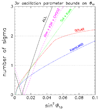
Figure 1.1: Global fits to $\sin^{2}\theta_{13}$, taken from [18].

Note that fits involving solar or atmospheric data separately have $\theta_{13}=0$ coinciding with the minima of the chi-square. However global analyses taking into account both solar and atmospheric effects show $\chi^{2}$ minima at a non-vanishing value of $\theta_{13}$. Another very recent global fit [19] with different inputs finds allowed ranges for the oscillation parameters that overlap significantly with the above results even at $1\sigma$ (68% C.L.). The latest MINOS neutrino oscillation results [9] significantly overlap those in the global fit [18]. All these signify the convergence to a set of accepted values of neutrino oscillation parameters $\Delta{m}^{2}_{21}$, $|\Delta{m}^{2}_{32}|$, $\sin^{2}\theta_{12}$, and $\sin^{2}\theta_{23}$.

At 95% C.L., the upper bound of $\theta_{13}$ extracted from Eq. 23 is about 10^∘. This corresponds to a value of $\sin^{2}2\theta_{13}$ of 0.12, which should be compared to the upper limit of 0.17 at 90% C.L. obtained by Chooz (see Section 1.6.1). We can conclude that, unlike $\theta_{12}$ and $\theta_{23}$, the mixing angle $\theta_{13}$ is relatively small.

At present the three parameters that are not determined by the solar, atmospheric, and KamLAND data are $\theta_{13}$, the sign of $\Delta m^{2}_{32}$ which fixes the hierarchy of neutrino masses, and the Dirac $CP$ phase $\delta_{CP}$.

1.3 Significance of the Mixing Angle $\theta_{13}$

As one of the six neutrino mass parameters measurable in neutrino oscillations, $\theta_{13}$ is important in its own right and for further studies of neutrino oscillations. In addition, $\theta_{13}$ is important in theoretical model building of the neutrino mass matrix, which can serve as a guide to the theoretical understanding of physics beyond the standard model. Therefore, on all considerations, it is highly desirable to significantly improve our knowledge on $\theta_{13}$ in the near future. The February 28, 2006 report of the Neutrino Scientific Assessment Group (NuSAG) [20], which advises the DOE Offices of Nuclear Physics and High Energy Physics and the National Science Foundation, and the APS multi-divisional study’s report on neutrino physics, the Neutrino Matrix [21], both recommend with high priority a reactor antineutrino experiment to measure sin${}^{2}2\theta_{13}$ at the level of 0.01.

1.3.1 Impact on the experimental program

The next generation of neutrino oscillation experiments has several important goals to achieve: to measure more precisely the mixing angles and mass-squared differences, to probe the matter effect, to determine the hierarchy of neutrino masses, and very importantly to determine the Dirac $CP$ phase. The mixing matrix element which provides the information on the $CP$ phase angle $\delta_{CP}$ appears always in the combination $U_{\rm e3}=\sin\theta_{13}e^{-i\delta_{CP}}$. If $\theta_{13}$ is zero then it is not possible to probe leptonic $CP$ violation in oscillation experiments. Given the known mixing angles $\theta_{12}$ and $\theta_{23}$ which are both sizable, we thus need to know the value of $\theta_{13}$ to a sufficient precision in order to design the future generation of experiments to measure $\delta_{CP}$. The matter effect, which can be used to determine the mass hierarchy, also depends on the size of $\theta_{13}$. If $\theta_{13}>0.01$, then the design of future oscillation experiments is relatively straightforward [22]. However, for smaller $\theta_{13}$ new experimental techniques and accelerator technologies are likely required to carry out the same sets of measurements.

1.3.2 Impact on theoretical development

The observation of neutrino oscillation has far reaching theoretical implications. To date, it is the only evidence of physics beyond the standard model in particle physics. The pattern of the neutrino mixing parameters revealed so far is strikingly different from that of quarks. This has already put significant constraints and guidance for constructing models involving new physics. Driven by the value of $\theta_{13}$, studies of the neutrino mass matrix have reached some interesting general conclusions.

In general, if $\theta_{13}$ is not too small i.e., close to the current upper limit of $\sin^{2}2\theta_{13}\approx 0.1$ and $\theta_{23}\neq{\pi\over 4}$, the neutrino mass matrix does not have to have any special symmetry features, sometimes referred to as anarchy models, and the specific values of the mixing angles can be understood as a numerical accident.

However, if $\theta_{13}$ is much smaller than the current limit, special symmetries of the neutrino mass matrix will be required. As a concrete example, the study of Mohapatra [23] shows that for $\theta_{13}<{\Delta{m}^{2}_{\rm sol}\over\Delta{m}^{2}_{\rm atm}}\approx 0.03$ a $\mu$-$\tau$ lepton-flavor-exchange symmetry is required. It disfavors a quark-lepton unification type theory based on $SU_{c}(4)$ or $SO(10)$ models.

For a larger value of $\theta_{13}$, it leaves open the question of quark-lepton unification.

1.4 Complementarity of Reactor-based and Accelerator-based Neutrino Oscillation Experiments

Long-baseline accelerator experiments with intense $\nu_{\mu}$ beams and very large detectors, in addition to improving the measurements of $|\Delta m^{2}_{32}|$ and $\theta_{23}$ via the study of $\nu_{\mu}$ survival, will also be able to search for $\nu_{e}$ appearance due to $\nu_{\mu}\to\nu_{e}$ oscillations. A measurement of both $\nu_{\mu}\to\nu_{e}$ and $\bar{\nu}_{\mu}\to\bar{\nu}_{e}$ oscillations allows one to measure $\theta_{13}$, test for $CP$ violation in the lepton sector, and determine the hierarchy of the neutrino masses, provided that $\theta_{13}$ is large enough. However, there are potentially three two-fold parameter degeneracies leading to the following ambiguities [1, 24]:

1. the $\delta_{CP}-\theta_{13}$ ambiguity,

2. the ambiguity in the sign of $\Delta m^{2}_{32}$ and

3. the $\theta_{23}$ ambiguity, which occurs because only $\sin^{2}2\theta_{23}$, not $\theta_{23}$, is measured in $\nu_{\mu}$ survival.

The degeneracies can all be present simultaneously, leading to as much as an eight-fold ambiguity in the determination of $\theta_{13}$ and $\delta_{CP}$. Another problem is that Earth-matter effects can induce fake $CP$ violation, which must be taken into account in any determination of $\theta_{13}$ and $\delta_{CP}$. One advantage of matter effects is that they may be able to distinguish between the two possible mass hierarchies.

There are experimental strategies that can overcome some of these problems. For example, by combining the results of two long-baseline experiments at different baselines, the sign of $\Delta m^{2}_{32}$ could be determined if $\theta_{13}$ is large enough [25]. By sitting near the peak of the leading oscillation with a narrow-band beam, $\theta_{13}$ can be removed from the $\delta_{CP}-\theta_{13}$ ambiguity [26]. However, neither of these approaches resolves the $\theta_{23}$ ambiguity, and $\theta_{13}$ may not be uniquely determined.

The $\bar{\nu}_{e}$ survival probability for reactor antineutrinos at short baseline depends only on $\theta_{13}$ and $\Delta m^{2}_{31}$, and is independent of $\delta_{CP}$ and insensitive to $\theta_{12}$ and $\Delta m_{21}^{2}$. Furthermore, matter effects are negligible due to the short distance. Therefore, a short-baseline reactor antineutrino experiment is an ideal method for measuring $\theta_{13}$ with no degeneracy problem. If $\theta_{13}$ can be unambiguously determined by a reactor antineutrino experiment, then the $\delta_{CP}-\theta_{13}$ ambiguity is resolved and long-baseline accelerator experiments can measure $\delta_{CP}$ and determine the sign of $\Delta m^{2}_{32}$ [27]. Figure 1.2 is an illustration of the synergy between reactor experiments and the future very long-baseline accelerator experiment, NOvA.

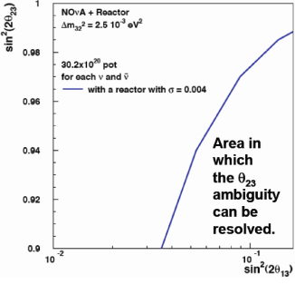
Figure 1.2: Resolving ambiguity in $\theta_{23}$ with $\sin^{2}2\theta_{13}$ determined by reactor experiments. Not only does the reactor experiment provide a precise measurement of $\sin^{2}2\theta_{13}$, but it provides a precise measurement of $\theta_{23}$ by resolving an ambiguity in the interpretation of the accelerator data. The blue line is the 95% C.L. curve averaged over the two mass-hierarchy solutions and possible values of $\delta_{CP}$.

For $\sin^{2}2\theta_{23}>0.87$ at 68% C.L. [9], using both muon neutrino and antineutrino beams, NOvA cannot distinguish the value of $\theta_{23}$. Yet, for $\Delta m^{2}_{32}=2.5\times 10^{-}3$ eV² and $\sin^{2}2\theta_{13}>0.035$, a reactor antineutrino experiment with an error of 0.004 can help single out the correct value for $\theta_{23}$.

1.5 Reactor Antineutrino Experiments

Nuclear reactors have played crucial roles in experimental neutrino physics. Most prominently, the very first observation of the neutrino was made at the Savannah River Nuclear Reactor in 1956 by Reines and Cowan [28], 26 years after the neutrino was first proposed. Recently, again using nuclear reactors, KamLAND observed disappearance of reactor antineutrinos at long baseline and distortion in the energy spectrum, strengthening the evidence of neutrino oscillation. Furthermore, as discussed in Section 1.4, reactor-based antineutrino experiments have the potential of uniquely determining $\theta_{13}$ at a low cost and in a timely fashion.

In this section we summarize the important features of nuclear reactors which are crucial to reactor-based antineutrino experiments.

1.5.1 Energy Spectrum and Flux of Reactor Antineutrinos

A nuclear power plant derives its power from the fission of uranium and plutonium isotopes (mostly ²³⁵U and ²³⁹Pu) which are embedded in the fuel rods in the reactor core. The fission produces daughters, many of which beta decay because they are neutron-rich. Each fission on average releases approximately 200 MeV of energy and six antineutrinos. The majority of the antineutrinos have very low energies; about 75% are below 1.8 MeV, the threshold of the inverse beta-decay reaction that will be discussed in Section 1.5.2. A typical reactor with 3 GW of thermal power (3 GW_th) emits $6\times 10^{20}$ antineutrinos per second with antineutrino energies up to 8 MeV.

Many reactor antineutrino experiments to date have been carried out at pressurized water reactors (PWRs). The antineutrino flux and energy spectrum of a PWR depend on several factors: the total thermal power of the reactor, the fraction of each fissile isotopes in the fuel, the fission rate of each fissile isotope, and the energy spectrum of antineutrinos of the individual fissile isotopes.

The antineutrino yield is directly proportional to the thermal power that is estimated by measuring the temperature, pressure and the flow rate of the cooling water. The reactor thermal power is measured continuously by the power plant with a typical precision of about 1%.

Fissile materials are continuously consumed while new fissile isotopes are produced from other fissionable isotopes in the fuel (mainly ²³⁸U) by fast neutrons. Since the antineutrino energy spectra are slightly different for the four main isotopes, ²³⁵U, ²³⁸U, ²³⁹Pu, and ²⁴¹Pu, the knowledge on the fission composition and its evolution over time are therefore critical to the determination of the antineutrino flux and energy spectrum. From the average thermal power and the effective energy released per fission [29], the average number of fissions per second of each isotope can be calculated as a function of time. Figure 1.3 shows the results of a computer simulation of the Palo Verde reactor cores [30].

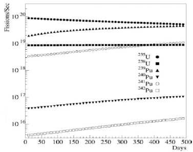
Figure 1.3: Fission rate of reactor isotopes as a function of time from a Monte Carlo simulation [30].

It is common for a nuclear power plant to replace some of the fuel rods in the core periodically as the fuel is used up. Typically, a core will have 1/3 of its fuel changed every 18 months. At the beginning of each refueling cycle, 69% of the fissions are from ²³⁵U, 21% from ²³⁹Pu, 7% from ²³⁸U, and 3% from ²⁴¹Pu. During operation the fissile isotopes ²³⁹Pu and ²⁴¹Pu are produced continuously from ²³⁸U. Toward the end of the fuel cycle, the fission rates from ²³⁵U and ²³⁹Pu are about equal. The average (“standard”) fuel composition is 58% of ²³⁵U, 30% of ²³⁹Pu, 7% of ²³⁸U, and 5% ²⁴¹Pu [31].

In general, the composite antineutrino energy spectrum is a function of the time-dependent contributions of the various fissile isotopes to the fission process. The Bugey 3 experiment compared three different models of the antineutrino spectrum with its measurement [32]. Good agreement was observed with the model that made use of the $\bar{\nu}_{e}$ spectra derived from the $\beta$ spectra [33] measured at the Institute Laue-Langevin (ILL). The ILL derived spectra for isotopes ²³⁵U, ²³⁹Pu, and ²⁴¹Pu are shown in Fig. 1.5.

Figure 1.4: Yield of antineutrinos per fission for the several isotopes. These are determined by converting the corresponding measured $\beta$ spectra [33].

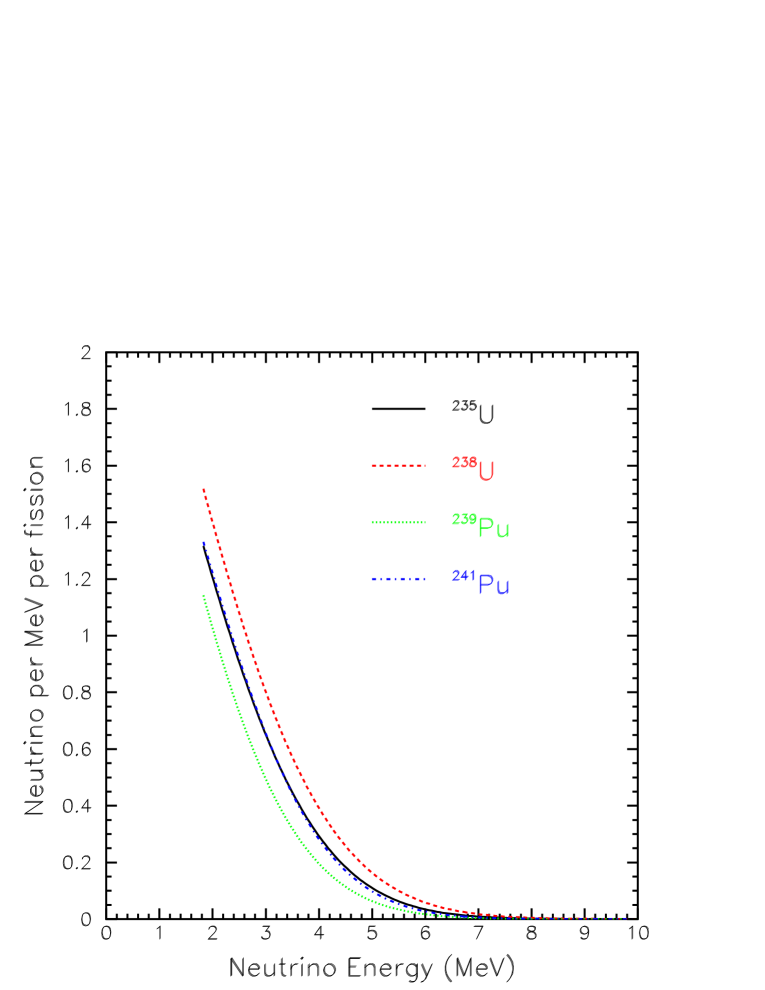
Figure 1.5: Antineutrino energy spectrum for four isotopes following the parameterization of Vogel and Engel [34].

However, there is no data for ²³⁸U; only the theoretical prediction is used. The possible discrepancy between the predicted and the real spectra should not lead to significant errors since the contribution from ²³⁸U is never higher than 8%. The overall normalization uncertainty of the ILL measured spectra is 1.9%. A global shape uncertainty is also introduced by the conversion procedure.

A widely used three-parameter parameterization of the antineutrino spectrum for the four main isotopes, as shown in Fig. 1.5, can be found in [34].

1.5.2 Inverse Beta-Decay Reaction

The reaction employed to detect the $\bar{\nu}_{e}$ from a reactor is the inverse beta-decay $\bar{\nu}_{e}+p\to e^{+}+n$. The total cross section of this reaction, neglecting terms of order $E_{\nu}/M$, where $E_{\nu}$ is the energy of the antineutrino and $M$ is the nucleon mass, is

$$\sigma^{(0)}_{tot}=\sigma_{0}(f^{2}+3g^{2})(E^{(0)}_{e}p^{(0)}_{e}/1{\rm MeV^{2}})$$ (24)

where $E^{(0)}_{e}=E_{\nu}-(M_{n}-M_{p})$ is the positron energy when neutron recoil energy is neglected, and $p^{(0)}_{e}$ is the positron momentum. The weak coupling constants are $f=1$ and $g=1.26$, and $\sigma_{0}$ is related to the Fermi coupling constant $G_{F}$, the Cabibbo angle $\theta_{C}$, and an energy-independent inner radiative correction. The inverse beta-decay process has a threshold energy in the laboratory frame $E_{\nu}=[(m_{\rm n}+m_{\rm e})^{2}-m^{2}_{\rm p}]/2m_{\rm p}$ = 1.806 MeV. The leading-order expression for the total cross section is

$$\sigma^{(0)}_{tot}=0.0952\times 10^{-42}{\rm cm}^{2}(E^{(0)}_{e}p^{(0)}_{e}/1{\rm MeV^{2}})$$ (25)

Vogel and Beacom [35] have recently extended the calculation of the total cross section and angular distribution to order $1/M$ for the inverse beta-decay reaction. Figure 1.6 shows the comparison of the total cross sections obtained in the leading order and the next-to-leading order calculations.

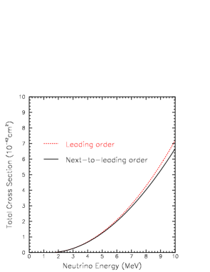
Figure 1.6: Total cross section for inverse beta-decay calculated in leading order and next-to-leading order.

Noticeable differences are present for high antineutrino energies. We adopt the order $1/M$ formulae for describing the inverse beta-decay reaction. The calculated cross section can be related to the neutron lifetime, whose uncertainty is only 0.2%.

The expected recoil neutron energy spectrum, weighted by the antineutrino energy spectrum and the $\bar{\nu}_{e}+p\to e^{+}+n$ cross section, is shown in Fig. 1.8.

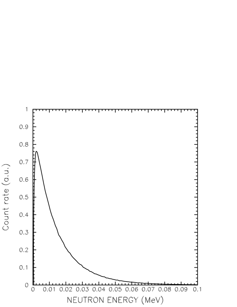
Figure 1.7: Recoil neutron energy spectrum from inverse beta-decay weighted by the antineutrino energy spectrum.

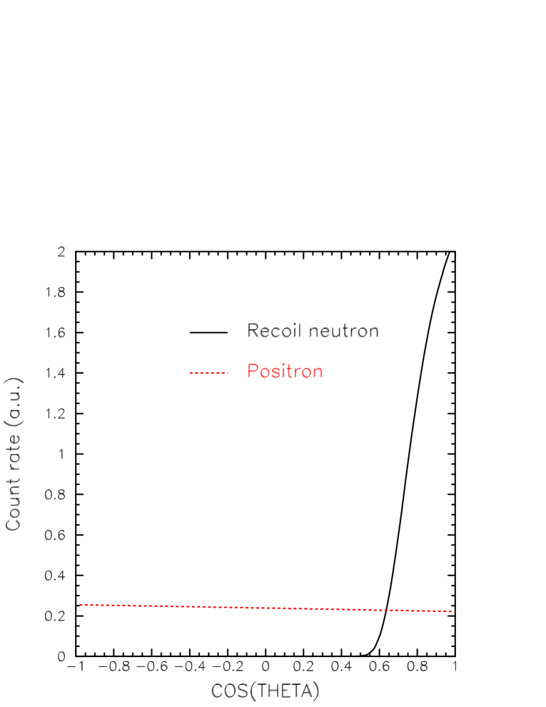
Figure 1.8: Angular distributions of positrons and recoil neutrons from inverse beta-decay in the laboratory frame.

Due to the low antineutrino energy relative to the mass of the nucleon, the recoil neutron has low kinetic energy. While the positron angular distribution is slightly backward peaked in the laboratory frame, the angular distribution of the neutrons is strongly forward peaked, as shown in Fig. 1.8.

1.5.3 Observed Antineutrino Rate and Spectrum at Short Distance

The observed antineutrino spectrum in a liquid scintillator detector, which is rich in free protons in the form of hydrogen, is a product of the reactor antineutrino spectrum and the cross section of inverse beta-decay. Figure 1.9 shows the differential antineutrino energy spectrum, the total cross section of the inverse beta-decay reaction, and the expected count rate as a function of the antineutrino energy. The differential energy distribution is the sum of the antineutrino spectra of all the radio-isotopes in the fuel. It is thus sensitive to the variation of thermal power and composition of the nuclear fuel.

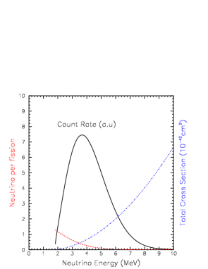
Figure 1.9: Antineutrino energy spectrum, total inverse beta-decay cross section, and count rate as a function of antineutrino energy.

By integrating over the energy of the antineutrino, the number of events can be determined. With one-ton of liquid scintillator, a typical rate is about 100 antineutrinos per day per GW_th at 100 m from the reactor. The highest count rate occurs at $E_{\nu}\sim 4$ MeV when there is no oscillation.

1.5.4 Reactor Antineutrino Disappearance Experiments

In a reactor-based antineutrino experiment the measured quantity is the survival probability for $\bar{\nu}_{\rm e}\rightarrow\bar{\nu}_{\rm e}$ at a baseline of the order of hundreds of meters to about a couple hundred kilometers with the $\bar{\nu}_{\rm e}$ energy from about 1.8 MeV to 8 MeV. The matter effect is totally negligible and so the vacuum formula for the survival probability is valid. In the notation of Eq. 20, this probability has a simple expression

$$P_{\rm sur} = 1-C^{4}_{13}\sin^{2}2\theta_{12}\sin^{2}\Delta_{21}-C^{2}_{12}\sin^{2}2\theta_{13}\sin^{2}\Delta_{31}-S^{2}_{12}\sin^{2}2\theta_{13}\sin^{2}\Delta_{32}$$ (26)

where

$$\Delta_{\rm jk} \equiv 1.267\Delta{m}^{2}_{\rm jk}({\rm eV^{2}})\times 10^{3}{L({\rm km})\over E({\rm MeV})}$$ (27)

$$\Delta{m}^{2}_{\rm jk} \equiv m^{2}_{\rm j}-m^{2}_{\rm k}$$

$L$ is the baseline in km, $E$ the antineutrino energy in MeV, and $m_{\rm j}$ the $j$-th antineutrino mass in eV. The $\nu_{\rm e}\rightarrow\nu_{\rm e}$ survival probability is also given by Eq. 26 when $CPT$ is not violated. Eq. 26 is independent of the $CP$ phase angle $\delta_{CP}$ and the mixing angle $\theta_{23}$.

To obtain the value of $\theta_{13}$, the depletion of $\bar{\nu}_{\rm e}$ has to be extracted from the experimental $\bar{\nu}_{\rm e}$ disappearance probability,

$$P_{\rm dis} \equiv 1-P_{\rm sur}$$ (28)

$$= C^{4}_{13}\sin^{2}2\theta_{12}\sin^{2}\Delta_{21}+C^{2}_{12}\sin^{2}2\theta_{13}\sin^{2}\Delta_{31}+S^{2}_{12}\sin^{2}2\theta_{13}\sin^{2}\Delta_{32}\,$$

Since $\theta_{13}$ is known to be less than 10^∘, we define the term that is insensitive to $\theta_{13}$ as

$$P_{12}=C^{4}_{13}\sin^{2}2\theta_{12}\sin^{2}\Delta_{21}\approx\sin^{2}2\theta_{12}\sin^{2}\Delta_{21}\,$$ (29)

Then the part of the disappearance probability directly related to $\theta_{13}$ is given by

$$P_{13} \equiv P_{\rm dis}-P_{12}$$ (30)

$$= +C^{2}_{12}\sin^{2}2\theta_{13}\sin^{2}\Delta_{31}+S^{2}_{12}\sin^{2}2\theta_{13}\sin^{2}\Delta_{32}$$

The above discussion shows that in order to obtain $\theta_{13}$ we have to subtract the $\theta_{13}$-insensitive contribution $P_{12}$ from the experimental measurement of $P_{\rm dis}$. To see their individual effect, we plot $P_{13}$ in Fig. 1.10

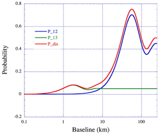
Figure 1.10: Reactor antineutrino disappearance probability as a function of distance from the source. The values of the mixing parameters are given in Eq. 31. $P_{12}$ is the slowly rising blue curve. $P_{13}$ is the green curve that has a maximum near 2 km. The total disappearance probability $P_{\rm dis}$ is the red curve.

together with $P_{\rm dis}$ and $P_{12}$ as a function of the baseline from 100 m to 250 km. The antineutrino energy is integrated from 1.8 MeV to 8 MeV. We also take $\sin^{2}2\theta_{13}=0.10$, which will be used for illustration in most of the discussions in this section. The other parameters are taken to be

$$\theta_{12}=34^{\circ},~{}~{}~{}\Delta{m}^{2}_{21}=7.9\times 10^{-5}{\rm eV}^{2},~{}~{}~{}\Delta{m}^{2}_{31}=2.5\times 10^{-3}{\rm eV}^{2}$$ (31)

The behavior of the curves in Fig. 1.10 are quite clear from their definitions, Eqs. (28), (29), and (30). Below a couple kilometers $P_{12}$ is very small, and $P_{13}$ and $P_{\rm dis}$ track each other well. This suggests that the measurement can be best performed at the first oscillation maximum of $P_{13}({\rm max})\simeq\sin^{2}2\theta_{13}$. Beyond the first minimum $P_{13}$ and $P_{\rm dis}$ deviate from each other more and more as $L$ increases when $P_{12}$ becomes dominant in $P_{\rm dis}$.

When we determine $P_{13}$(max) from the difference $P_{\rm dis}-P_{12}$, the uncertainties on $\theta_{12}$ and $\Delta m^{2}_{21}$ will propagate to $P_{13}$. It is easy to check that, given the best fit values in Eq. 21, when $\sin^{2}2\theta_{13}$ varies from 0.01 to 0.10 the relative size of $P_{12}$ compared to $P_{13}$ is about 25% to 2.6% at the first oscillation maximum. Yet the uncertainty in determining $\sin^{2}2\theta_{13}$ due to the uncertainty of $P_{12}$ is always less than 0.005.

In Fig. 1.11 $P_{13}$ integrated over $E$ from 1.8 to 8 MeV is shown as a function of $L_{\rm far}$, the best possible distance for the detector, for three values of $\Delta{m}^{2}_{32}$ that cover the allowed range of $\Delta{m}^{2}_{32}$ at 95% C.L. as given in Eq. 22.

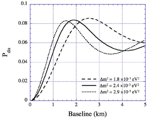
Figure 1.11: Reactor antineutrino disappearance probability due to the mixing angle $\theta_{13}$ as a function of the baseline $L_{\rm far}$ over the allowed 2$\sigma$ range in $\Delta{m}^{2}_{32}$.

The curves show that $P_{dis}$ is sensitive to $\Delta{m}^{2}_{32}$. For $\Delta{m}^{2}_{32}=(1.8,~{}2.4,~{}2.9)\times 10^{-3}$ eV², the oscillation maxima correspond to a baseline of 2.5 km, 1.9 km, and 1.5 km, respectively. From this simple study, placing the detector between 1.5 km and 2.5 km from the reactor looks to be a good choice.

We conclude from this phenomenological investigation that the choice of $L_{\rm far}$ be made so that it can cover as large a range of $\Delta{m}^{2}_{31}$ as possible.

1.6 Determining $\theta_{13}$ with Nuclear Reactors

In this section previous attempts to measure $\sin^{2}2\theta_{13}$ are summarized, and a new method for a high-precision determination of $\sin^{2}2\theta_{13}$ is presented.

1.6.1 Past Measurements

In the 1990’s, two reactor-based antineutrino experiments, Chooz [10] and Palo Verde [11], were carried out to investigate neutrino oscillation. Based on $\Delta{m}_{32}^{2}$ = $1.5\times 10^{-2}$ eV² as reported by Kamiokande [36], the baselines of Chooz and Palo Verde were chosen to be about 1 km. This distance corresponded to the location of the first oscillation maximum of $\nu_{e}\to\nu_{\mu}$ when probed with low-energy reactor $\bar{\nu}_{e}$. Both Chooz and Palo Verde were looking for a deficit in the $\bar{\nu}_{e}$ rate at the location of the detector by comparing the observed rate with the calculated rate assuming no oscillation occurred. With only one detector, both experiments had to rely on the operational information from the reactors, in particular, the composition of the nuclear fuel and the amount of thermal power generated as a function of time, for calculating the rate of $\bar{\nu}_{e}$ produced in the fission processes.

Chooz and Palo Verde utilized Gd-doped liquid scintillator (0.1% Gd by weight) to detect the reactor $\bar{\nu}_{e}$ via the inverse beta-decay $\bar{\nu}_{e}+p\to n+e^{+}$ reaction. The ionization loss and subsequent annihilation of the positron give rise to a fast signal obtained with photomultiplier tubes (PMTs). The energy associated with this signal is termed the prompt energy, $E_{p}$. As stated in Section 1.5.2, $E_{p}$ is directly related to the energy of the incident $\bar{\nu}_{e}$. After a typical moderation time of about 30 $\mu$s, the neutron is captured by a Gd nucleus, emitting several $\gamma$-ray photons with a total energy of about 8 MeV. This signal is called the delayed energy, $E_{d}$. The temporal correlation between the prompt energy and the delayed energy constitutes a powerful tool for identifying the $\bar{\nu}_{e}$ and for suppressing backgrounds.

The value of $\sin^{2}{2\theta_{13}}$ was determined by comparing the observed antineutrino rate and energy spectrum at the detector with the predictions that assumed no oscillation. The number of detected antineutrinos $N_{det}$ is given by

$$N_{\rm det} = \frac{N_{p}}{4\pi L^{2}}\int{\epsilon\sigma P_{\rm sur}SdE}$$ (32)

where $N_{p}$ is the number of free protons in the target, $L$ is the distance of the detector from the reactor, $\epsilon$ is the efficiency of detecting an antineutrino, $\sigma$ is the total cross section of the inverse beta-decay process, $P_{sur}$ is the survival probability given in Eq. 26, and $S$ is the differential energy distribution of the antineutrino at the reactor shown in Fig. 1.9.

Since the signal rate is low, it is desirable to conduct reactor-based antineutrino experiments underground to reduce cosmic-ray induced backgrounds, such as neutrons and the radioactive isotope ⁹Li. Gamma rays originating from natural radioactivity in construction materials and the surrounding rock are also problematic. The random coincidence of a $\gamma$ ray interaction in the detector followed by a neutron capture is a potential source of background. For Chooz, their background rate was $1.41\pm 0.24$ events per day in the 1997 run, and $2.22\pm 0.14$ events per day after the trigger was modified in 1998. The background events were subtracted from $N_{\rm det}$ before $\sin^{2}{2\theta_{13}}$ was extracted.

The systematic uncertainties and efficiencies of Chooz are summarized in Tables 1.1

parameter	relative uncertainty (%)
reaction cross section	1.9
number of protons	0.8
detection efficiency	1.5
reactor power	0.7
energy released per fission	0.6
combined	2.7

Table 1.1: Contributions to the overall systematic uncertainty in the absolute normalization of Chooz.

and 1.2 respectively.

selection	$\epsilon$ (%)	relative error (%)
positron energy	97.8	0.8
positron-geode distance	99.9	0.1
neutron capture	84.6	1.0
capture energy containment	94.6	0.4
neutron-geode distance	99.5	0.1
neutron delay	93.7	0.4
positron-neutron distance	98.4	0.3
neutron multiplicity	97.4	0.5
combined	69.8	1.5

Table 1.2: Summary of the antineutrino detection efficiency in Chooz.

Neither Chooz nor Palo Verde observed any deficit in the $\bar{\nu}_{e}$ rate. This null result was used to set a limit on the neutrino mixing angle $\theta_{13}$, as shown in Fig. 1.12.

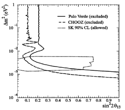
Figure 1.12: Exclusion contours determined by Chooz, Palo Verde along with the allowed region obtained by Kamiokande. [10]

Chooz obtained the best limit of 0.17 in sin${}^{2}2\theta_{13}$ for $\Delta{m}^{2}_{31}=2.5\times 10^{-3}$ eV² at the 90% confidence level.

1.6.2 Precision Measurement of $\theta_{13}$

With only one detector at a fixed baseline from a reactor, according to Eq. 32, Chooz and Palo Verde had to determine the absolute antineutrino flux from the reactor, the absolute cross section of the inverse beta-decay reaction, and the efficiencies of the detector and event-selection requirements in order to measure $\sin^{2}2\theta_{13}$. The prospect for determining $\sin^{2}2\theta_{13}$ precisely with a single detector that relies on a thorough understanding of the detector and the reactor is not promising. It is a challenge to reduce the systematic uncertainties of such an absolute measurement to sub-percent level, especially for reactor-related uncertainties.

Mikaelyan and Sinev pointed out that the systematic uncertainties can be greatly suppressed or totally eliminated when two detectors positioned at two different baselines are utilized [37]. The near detector close to the reactor core is used to establish the flux and energy spectrum of the antineutrinos. This relaxes the requirement of knowing the details of the fission process and operational conditions of the reactor. In this approach, the value of $\sin^{2}2\theta_{13}$ can be measured by comparing the antineutrino flux and energy distribution observed with the far detector to those of the near detector after scaling with distance squared. According to Eq. 32, the ratio of the number of antineutrino events with energy between $E$ and $E+dE$ detected at distance $L_{\rm f}$ to that at a baseline of $L_{\rm n}$ is given by

$$\frac{N_{\rm f}}{N_{\rm n}} = \left(\frac{N_{\rm p,f}}{N_{\rm p,n}}\right)\left(\frac{L_{\rm n}}{L_{\rm f}}\right)^{2}\left(\frac{\epsilon_{\rm f}}{\epsilon_{\rm n}}\right)\left[\frac{P_{\rm sur}(E,L_{\rm f})}{P_{\rm sur}(E,L_{\rm n})}\right]$$ (33)

If the detectors are made identical and have the same efficiency, the ratio depends only on the distances and the survival probabilities. By placing the near detector close to the core such that there is no significant oscillating effect, $\sin^{2}2\theta_{13}$ is approximately given by

$$\sin^{2}2\theta_{13} \approx \frac{1}{A(E,L_{\rm f})}\left[1-\left(\frac{N_{\rm f}}{N_{\rm n}}\right)\left(\frac{L_{\rm f}}{L_{\rm n}}\right)^{2}\right]$$ (34)

where $A(E,L_{\rm f})$ = $\sin^{2}\Delta_{31}$ with $\Delta_{31}$ defined in Eq. 27 is the analyzing power when the contribution of $\theta_{12}$ is small. Indeed, from this simplified picture, it is clear that the two-detector scheme is an excellent approach for pin-pointing the value of $\sin^{2}2\theta_{13}$ precisely. In practice, we need to extend this idea to handle more complicated arrangements involving multiple reactors and multiple detectors as in the case of the Daya Bay experiment.

1.7 The Daya Bay Reactor Antineutrino Experiment

As discussed in Section 1.5.4, probing $\sin^{2}2\theta_{13}$ with excellent sensitivity will be an important milestone in advancing neutrino physics. There are proposals to explore $\sin^{2}2\theta_{13}$ with sensitivities approaching the level of 0.01 [22]. The objective of the Daya Bay experiment is to determine $\sin^{2}2\theta_{13}$ with sensitivity of 0.01 or better.

In order to reach the designed goal, it is important to reduce both the statistical and systematic uncertainties as well as suppress backgrounds to comparable levels in the Daya Bay neutrino oscillation experiment.

This experiment will be located at the Daya Bay nuclear power complex in southern China. Its geographic location is shown in Fig. 1.13.

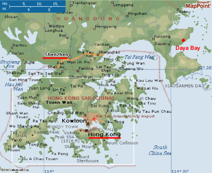
Figure 1.13: Daya Bay and vicinity: The nuclear power complex is located about 55 km from central Hong Kong.

The experimental site is about 55 km north-east from Victoria Harbor in Hong Kong. Figure 1.14

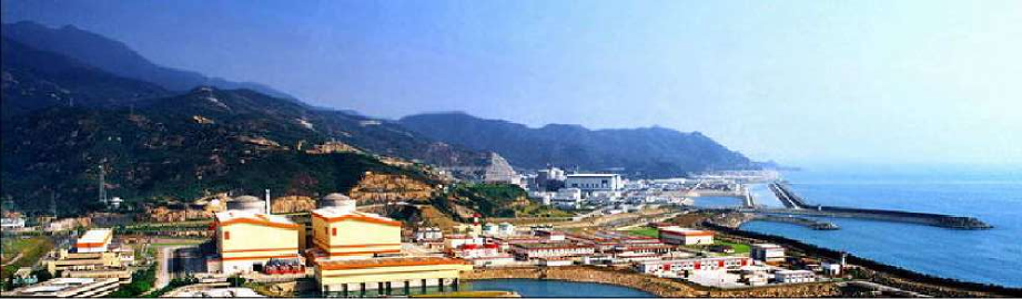
Figure 1.14: The Daya Bay nuclear power complex. The Daya Bay nuclear power plant is in the foreground. The Ling Ao nuclear power plant is in the background. The experimental halls will be underneath the hills to the left.

is a photograph of the complex. The complex consists of three nuclear power plants (NPPs): the Daya Bay NPP, the Ling Ao NPP, and the Ling Ao II NPP. The Ling Ao II NPP is under construction and will be operational by 2010–2011. Each plant has two identical reactor cores. Each core generates 2.9 GW_th during normal operation. The Ling Ao cores are about 1.1 km east of the Daya Bay cores, and about 400 m west of the Ling Ao II cores. There are mountain ranges to the north which provide sufficient overburden to suppress cosmogenic backgrounds in the underground experimental halls. Within 2 km of the site the elevation of the mountain varies generally from 185 m to 400 m.

The six cores can be roughly grouped into two clusters, the Daya Bay cluster of two cores and the Ling Ao cluster of four cores. We plan to deploy two identical sets of near detectors at distances between 300 m and 500 m from their respective cluster of cores to monitor the antineutrino fluxes. Another set of identical detectors, called the far detectors, will be located approximately 1.5 km north of the two near detector sets. Since the overburden of the experimental site increases with distance from the cores, the cosmogenic background decreases as the signal decreases, hence keeping the background-to-signal ratio roughly constant. This is beneficial to controlling systematic uncertainties. By comparing the antineutrino fluxes and energy spectra between the near and far detectors, the Daya Bay experiment will determine $\sin^{2}2\theta_{13}$ to the designed sensitivity. Detailed design of the experiment, including baseline optimization accounting for statistical and systematic uncertainty, backgrounds and topographical information will be discussed in the following chapters.

It is possible to instrument a mid detector site between the near and far sites. The mid detectors along with the near and far detectors can be used to carry out measurements for systematic studies and for internal consistency checks. In combination with the near detectors close to the Daya Bay NPP, they could also be utilized to provide a quick determination of $\sin^{2}{2\theta_{13}}$, albeit with reduced sensitivity, in the early stage of the experiment.

2 Experimental Design Overview

To establish the existence of neutrino oscillation due to $\theta_{13}$, and to determine sin${}^{2}2\theta_{13}$ to a precision of 0.01 or better, at least 50,000 detected events detected at the far site are needed, and systematic uncertainties in the ratios of near-to-far detector acceptance, antineutrino flux and background have to be controlled to a level below 0.5%, an improvement of almost an order of magnitude over the previous experiments. Based on recent single detector reactor experiments such as Chooz, Palo Verde and KamLAND, there are three main sources of systematic uncertainty: reactor-related uncertainty of (2–3)%, background-related uncertainty of (1–3)%, and detector-related uncertainty of (1–3)%. Each source of uncertainty can be further classified into correlated and uncorrelated uncertainties. Hence a carefully designed experiment, including the detector design and background control, is required. The primary considerations driving the improved performance are listed below:

• identical near and far detectors Use of identical detectors at the near and far sites to cancel reactor-related systematic uncertainties, a technique first proposed by Mikaelyan et al. for the Kr2Det experiment in 1999 [1]. The event rate of the near detector will be used to predict the yield at the far detector. Even in the case of a multiple reactor complex, reactor-related uncertainties can be controlled to negligible level by a careful choice of locations of the near and far sites.

• multiple modules Employ multiple, identical modules at the near and far sites to cross check between modules at each location and reduce detector-related uncorrelated uncertainties. The use of multiple modules in each site enables internal consistency check to the limit of statistics. Multiple modules implies smaller detectors which are easier to move. In addition, small modules intercept fewer cosmic-ray muons, resulting in less dead time, less cosmogenic background and hence smaller systematic uncertainty. Taking calibration and monitoring of detectors, redundancy, and cost into account we settle on a design with two modules for each near site and four modules for the far site.

• three-zone detector module Each module is partitioned into three enclosed zones. The innermost zone, filled with Gd-loaded liquid scintillator, is the antineutrino target which is surrounded by a zone filled with unloaded liquid scintillator called the $\gamma$-catcher. This middle zone is used to capture the $\gamma$ rays from antineutrino events that leak out of the target. This arrangement can substantially reduce the systematic uncertainties related to the target volume and mass, positron energy threshold, and position cut. The outermost zone, filled with transparent mineral oil that does not scintillate, shields against external $\gamma$ rays entering the active scintillator volume.

• sufficient overburden and shielding Locations of all underground detector halls are optimized to ensure sufficient overburden to reduce cosmogenic backgrounds to the level that can be measured with certainty. The antineutrino detector modules are enclosed with sufficient passive shielding to attenuate natural radiation and energetic spallation neutrons from the surrounding rocks and materials used in the experiment.

• multiple muon detectors By tagging the incident muons, the associated cosmogenic background events can be suppressed to a negligible level. This will require the muon detector to have a high efficiency and that it is known with small uncertainty. Monte Carlo study shows that the efficiency of the muon detector should be better than 99.5% (with an uncertainty less than 0.25%). The muon system is designed to have at least two detector systems. One system utilizes the water buffer as a Cherenkov detector, and another employs muon tracking detectors with decent position resolution. Each muon detector can easily be constructed with an efficiency of (90–95)% such that the overall efficiency of the muon system will be better than 99.5%. In addition, the two muon detectors can be used to measure the efficiency of each other to a uncertainty of better than 0.25%.

• movable detectors The detector modules are movable, such that swapping of modules between the near and far sites can be used to cancel detector-related uncertainties to the extent that they remain unchanged before and after swapping. The residual uncertainties, being secondary, are caused by energy scale uncertainties not completely taken out by calibration, as well as other site-dependent uncertainties. The goal is to reduce the systematic uncertainties as much as possible by careful design and construction of detector modules such that swapping of detectors is not necessary. Further discussion of detector swapping will be given in Chapters 3 and 10.

With these improvements, the total detector-related systematic uncertainty is expected to be $\sim$0.2% in the near-to-far ratio per detector site which is comparable to the statistical uncertainty of $\sim$0.2% (based on the expected 250,000 events for three years of running at the far site). Using a global $\chi^{2}$ analysis (see Section 3.5.1), incorporating all known systematic and statistical uncertainties, we find that $\sin^{2}2\theta_{13}$ can be determined to a sensitivity of better than 0.01 at 90% confidence level as discussed in Sec. 3.5.2.

2.1 Experimental layout

Taking the current value of $\Delta m^{2}_{31}=2.5\times 10^{-3}$ eV² (see equation 31), the first maximum of the oscillation associated with $\theta_{13}$ occurs at $\sim$1800 m. Considerations based on statistics alone will result in a somewhat shorter baseline, especially when the statistical uncertainty is larger than or comparable to the systematic uncertainty. For the Daya Bay experiment, the overburden influences the optimization since it varies along the baseline. In addition, a shorter tunnel will decrease the civil construction cost.

The Daya Bay experiment will use identical detectors at the near and far sites to cancel reactor-related systematic uncertainties, as well as part of the detector-related systematic uncertainties. The Daya Bay site currently has four cores in two groups: the Daya Bay NPP and the Ling Ao NPP. The two Ling Ao II cores will start to generate electricity in 2010–2011. Figure 2.1 shows the locations of all six cores.

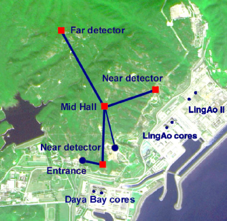
Figure 2.1: Layout of the Daya Bay experiment.

The distance between the two cores in each NPP is about 88 m. Daya Bay is 1100 m from Ling Ao, and the maximum distance between cores will be 1600 m when Ling Ao II starts operation. The experiment will locate detectors close to each reactor cluster to monitor the antineutrinos emitted from their cores as precisely as possible. At least two near sites are needed, one is primarily for monitoring the Daya Bay cores and the other primarily for monitoring the Ling Ao—Ling Ao II cores. The reactor-related systematic uncertainties can not be cancelled exactly, but can be reduced to a negligible revel, as low as 0.04% if the overburden is not taken into account. A global optimization taking all factors into account, especially balancing the overburden and reactor-related uncertainties, results in a residual reactor uncertainty of $<$0.1%

Three major factors are involved in optimizing the locations of the near sites. The first one is overburden. The slope of the hills near the site is around 30 degrees. Hence, the overburden falls rapidly as the detector site is moved closer to the cores. The second concern is oscillation loss. The oscillation probability is appreciable even at the near sites. For example, for the near detectors placed approximately 500 m from the center of gravity of the cores, the integrated oscillation probability is $0.19\times\sin^{2}2\theta_{13}$ (computed with $\Delta m_{31}^{2}=2.5\times 10^{-3}$ eV²). The oscillation contribution of the other pair of cores, which is around 1100 m away, has been included. The third concern is the near-far cancellation of reactor uncertainties.

After careful study of many different experimental designs, the best configuration of the experiment is shown in Fig. 2.1 together with the tunnel layout. Based on this configuration, a global $\chi^{2}$ fit (see Eq. 48) for the best sensitivity and baseline optimization was performed, taking into account backgrounds, mountain profile, detector systematics and residual reactor related uncertainties. The result is shown in Fig. 2.2.

Figure 2.2: Site optimization using the global $\chi^{2}$ analysis. The optimal sites are labelled with red triangles. The stars show the reactors. The black contours show the sensitivity when one site’s location is varied and the other two are fixed at optimal sites. The red lines with tick marks are the perpendicular bisectors of the reactor pairs. The mountain contours are also shown on the plot (blue lines).

Ideally each near detector site should be positioned equidistant from the cores that it monitors so that the uncorrelated reactor uncertainties are cancelled. However, taking overburden and statistics into account while optimizing the experimental sensitivity, the Daya Bay near detector site is best located 363 m from the center of the Daya Bay cores. The overburden at this location is 98 m (255 m.w.e.). The Ling Ao near detector hall is optimized to be 481 m from the center of the Ling Ao cores, and 526 m from the center of the Ling Ao II cores where the overburden is 112 m (291 m.w.e).

The far detector site is about 1.5 km north of the two near sites. Ideally the far site should be equidistant between the Daya Bay and Ling Ao—Ling Ao II cores; however, the overburden at that location would be only 200 m (520 m.w.e). At present, the distances from the far detector to the midpoint of the Daya Bay cores and to the mid point of the Ling Ao—Ling Ao II cores are 1985 m and 1615 m, respectively. The overburden is about 350 m (910 m.w.e). A summary of the distances to each detector is provided in Table 2.1.

Sites	DYB	LA	Far
DYB cores	363	1347	1985
LA cores	857	481	1618
LA II cores	1307	526	1613

Table 2.1: Distances in meters from each detector site to the centroid of each pair of reactor cores.

It is possible to install a mid detector hall between the near and far sites such that it is 1156 m from the midpoint of the Daya Bay cores and 873 m from the center of the Ling Ao—Ling Ao II cores. The overburden at the mid hall is 208 m (540 m.w.e.). This mid hall could be used for a quick measurement of $\sin^{2}2\theta_{13}$, studies of systematics and internal consistency checks.

There are three branches for the main tunnel extending from a junction near the mid hall to the near and far underground detector halls. There are also access and construction tunnels. The length of the access tunnel, from the portal to the Daya Bay near site, is 295 m. It has a grade between 8% and 12% [2]. A sloped access tunnel allows the underground facilities to be located deeper with more overburden. The quoted overburdens are based on a 10% grade.

2.2 Detector Design

As discussed above, the antineutrino detector employed at the near (far) site has two (four) modules while the muon detector consists of a cosmic-ray tracking device and active water buffer. There are several possible configurations for the water buffer and the muon tracking detector as discussed in Section 7. The baseline design is shown in Fig. 2.3.

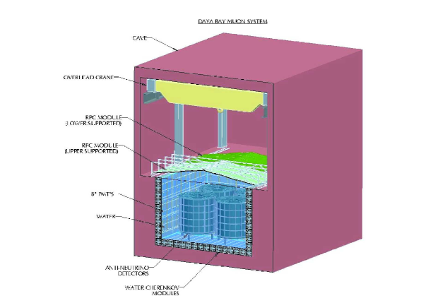
Figure 2.3: Layout of the baseline design of the Daya Bay detector. Four antineutrino detector modules are shielded by a 1.5 m-thick active water Cherenkov buffer. Surrounding this buffer is another 1-meter of water Cherenkov tanks serving as muon trackers. The muon system is completed with RPCs at the top.

The water buffer in this case is a water pool, equipped with photomultiplier tubes (PMTs) to serve as a Cherenkov detector. The outer region of the water pool is segmented into water tanks made of reflective PVC sheets with a cross section of 1 m$\times$1 m and a length of 16 m. Four PMTs at each end of the water tank are installed to collect Cherenkov photons produced by cosmic muons in the water tank. The water tank scheme first proposed by Y.F. Wang [3] for very long baseline neutrino experiments as a segmented calorimeter is a reasonable choice as a muon tracking detector for reasons of both cost and technical feasibility. Above the pool the muon tracking detector is made of light-weight resistive-plate chambers (RPCs). RPCs offer good performance and excellent position resolution for low cost.

The antineutrino detector modules are submerged in the water pool that shields the modules from ambient radiation and spallation neutrons. Other possible water shielding configurations will be discussed in Section 2.3.

2.2.1 Antineutrino detector

Antineutrinos are detected by an organic liquid scintillator (LS) with high hydrogen content (free protons) via the inverse beta-decay reaction:

$$\bar{\nu}_{e}+p\longrightarrow e^{+}+n$$

The prompt positron signal and delayed neutron-capture signal are combined to define a neutrino event with timing and energy requirements on both signals. In LS neutrons are captured by free protons in the scintillator emitting 2.2 MeV $\gamma$-rays with a capture time of 180 $\mu$s. On the other hand, when Gadolinium (Gd), with its huge neutron-capture cross section and subsequent 8 MeV release of $\gamma$-ray energy, is loaded into LS the much higher $\gamma$ energy cleanly separates the signal from natural radioactivity, which is mostly below 2.6 MeV, and the shorter capture time ($\sim$30 $\mu$s) reduces the background from accidental coincidences. Both Chooz [4] and Palo Verde [5] used 0.1% Gd-loaded LS that yielded a capture time of 28 $\mu$s, about a factor of seven shorter than in undoped liquid scintillator. Backgrounds from random coincidences will thus be reduced by a factor of seven as compared to unloaded LS.

The specifications for the design of the antineutrino detector module follow:

• Employ three-zone detector modules partitioned with acrylic tanks as shown in fig 2.4.

  

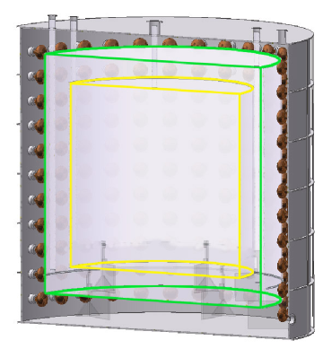
  Figure 2.4: Cross sectional slice of a 3-zone antineutrino detector module showing the acrylic vessels holding the Gd-doped liquid scintillator at the center (20 T), liquid scintillator between the acrylic vessels (20 T) and mineral oil (40 T) in the outer region. The PMTs are mounted on the inside walls of the stainless steel tank.

  The target volume is defined by the physical dimensions of the central region of Gd-loaded liquid scintillator. This target volume is surrounded by an intermediate region filled with normal LS to catch $\gamma$s escaping from the central region. The liquid-scintillator regions are embedded in a volume of mineral oil to separate the PMTs from the scintillator and suppress natural radioactivity from the PMT glass and other external sources.

  Four of these modules, each with 20 T fiducial volume, will be deployed at the far site to obtain sufficient statistics and two modules will be deployed at each near site, enabling cross calibrations. The matching of four near and four far detectors allows for analyzing data with matched near-far pairs.

  In this design, the homogeneous target volume is well determined without a position cut since neutrinos captured in the unloaded scintillator will not in general satisfy the neutron energy requirement. Each vessel will be carefully measured to determine its volume and each vessel will be filled with the same set of mass-flow and flow meters to minimize any variation in relative detector volume and mass. The effect of neutron spill-in and spill-out across the boundary between the two liquid-scintillator regions will be cancelled when pairs of identical detector modules are used at the near and far sites. With the shielding of mineral oil, the singles rate will be reduced substantially. The trigger threshold can thus be lowered to below 1.0 MeV, providing $\sim$100% detection efficiency for the prompt positron signal.

• The Gd-loaded liquid scintillator, which is the antineutrino target, should have the same composition and fraction of hydrogen (free protons) for each pair of detectors (one at a near site and the other at the far site). The detectors will be filled in pairs (one near and one far detector) from a common storage vessel to assure that the composition is the same. Other detector components such as unloaded liquid scintillator and PMTs will be characterized and distributed evenly to a pair of detector modules during assembly to equalize the properties of the modules.

• The energy resolution should be better than 15% at 1 MeV. Good energy resolution is desirable for reducing the energy-related systematic uncertainty on the neutron energy cut. Good energy resolution is also important for studying spectral distortion as a signature of neutrino oscillations.

• The time resolution should be better than 1 ns for determining the event time and for studying backgrounds.

Detector modules of different shapes, including cubical, cylindrical, and spherical, have been considered. From the point of view of ease of construction cubical and cylindrical shapes are particularly attractive. Monte Carlo simulation shows that modules of cylindrical shape can provide better energy and position resolutions for the same number of PMTs. Figure 2.4 shows the structure of a cylindrical module. The PMTs are arranged along the circumference of the outer cylinder. The surfaces at the top and the bottom of the outer-most cylinder are coated with white reflective paint or other reflective materials to provide diffuse reflection. Such an arrangement is feasible since 1) the event vertex is determined only with the center of gravity of the charge, not relying on the time-of-flight information, 2) the fiducial volume is well defined with a three-zone structure, thus no accurate vertex information is required. Details of the antineutrino detector will be discussed in Chapter 5.

2.2.2 Muon detector

Since most of the backgrounds come from the interactions of cosmic-ray muons with nearby materials, it is desirable to have a very efficient active muon detector coupled with a tracker for tagging the cosmic-ray muons. This will provide a means for studying and rejecting cosmogenic background events. The three detector technologies that are being considered are water Cherenkov counter, resistive plate chamber (RPC), and plastic scintillator strip. When the water Cherenkov counter is combined with a tracker, the muon detection efficiency can be close to 100%. Furthermore, these two independent detectors can cross check each other. Their inefficiencies and the associated uncertainties can be well determined by cross calibration during data taking. We expect the inefficiency will be lower than 0.5% and the uncertainty of the inefficiency will be lower than 0.25%.

Besides being a shield against ambient radiation, the water buffer can also be utilized as a water Cherenkov counter by installing PMTs in the water. The water Cherenkov detector is based on proven technology, and known to be very reliable. With sufficient PMT coverage and reflective surfaces, the efficiency of detecting muons should exceed 95%. The current baseline design of the water buffer is a water pool, similar to a swimming pool with a dimensions of 16 m (length) $\times$ 16 m (width) $\times$ 10 m (height) for the far hall containing four detector modules, as shown in Fig. 2.5.

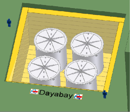
Figure 2.5: The water pool with four antineutrino detector modules inside. water tanks of dimension 1 m$\times$1 m are used as an outer muon tracker.

The PMTs of the water Cherenkov counters are mounted facing the inside of the water pool. This is a simple and proven technology with very limited safety concerns. The water will effectively shield the antineutrino detectors from radioactivity in the surrounding rocks and from Radon, with the attractive features of being simple, cost-effective and having a relatively short construction time.

The muon tracking detector consists of water tanks and RPCs. RPCs are very economical for instrumenting large areas, and simple to fabricate. The Bakelite based RPC developed by IHEP for the BES-III detector has a typical efficiency of 95% and noise rate of 0.1 Hz/cm² per layer. [6]. A possible configuration is to build three layers of RPC, and require two out of three layers hit within a time window of 20 ns to define a muon event. Such a scheme has an efficiency above 99% and noise rate of $<$0.1 Hz/m². Although RPCs are an ideal large area muon detector due to their light weight, good performance, excellent position resolution and low cost, it is hard to put them inside water to fully surround the water pool. The best choice seems to use them only at the top of the water pool.

Water tanks with a dimension of 1 m$\times$1 m and a length of 16 m as the outer muon tracking detector have a typical position resolution of about 30 cm. Although not as good as other choices, the resolution is reasonably good for our needs, in particular with the help of RPCs at the top. Actually the water tanks are not really sealed tanks, but reflective PVC sheets assembled on a stainless steel structure, so that water can flow freely among water pool and water tanks, and only one water purification system is needed for each site. Water tanks can be easily installed at the side of the water pool, but must be cut into sections at the bottom to leave space for the supporting structure of antineutrino detector modules. Each tank will be equipped with four PMTs at each end to collect Cherenkov photons produced by cosmic-muons. A few more PMTs are needed for the bottom tanks to take into account optical path obstruction by the supporting structure of the antineutrino detector modules. A 13 m long prototype has been built and tested [3]. A detailed Monte Carlo simulation based on the data from this prototype shows that the total light collected at each end is sufficient, as will be discussed in detail in Chapter 7. The technology employed in this design is mature and the detector is relatively easy and fast to construct.

2.3 Alternative Designs of the Water Buffer

We have chosen a water pool as the baseline experimental design (see Fig. 2.3). The two near detector sites have two antineutrino detector modules in a rectangular water pool, whereas the far site has four antineutrino detector modules in a square water pool. The distance from the outer surface of each antineutrino detector is at least 2.5 m to the water surface, with 1 m of water between each antineutrino detector.

Our primary alternative to the baseline design is the “aquarium” option. A conceptual design, showing a cut-away side view is provided in Fig. 2.6.

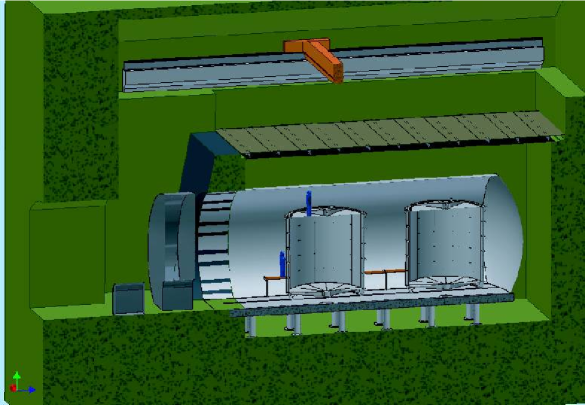
Figure 2.6: Side cutaway view of a near detector site aquarium with two detectors visible.

Several views are shown in Fig. 2.7.

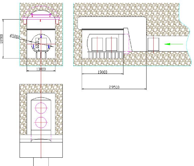
Figure 2.7: End, side and top views of the conceptual design of a near detector site aquarium. All distances are in mm.

The primary feature of this aquarium design is that the antineutrino detector modules do not sit in the water volume, but are rather in air. The advantages of this design are ease of access to the antineutrino detectors, ease of connections to the antineutrino detectors, simpler movement of the antineutrino detectors, more flexibility to calibrate the antineutrino detectors and a muon system that does not need to be partially disassembled or moved when the antineutrino detectors are moved. The primary disadvantages of this design include the engineering difficulties of the central tube and the water dam, safety issues associated with the large volume of water above the floor level, cost, maintenance of the antineutrino detectors free of radon and radioactive debris. This is preserved as the primary option for a “dry detector” and serves as our secondary detector design option. Other designs that have been considered include: ship-lock, modified aquarium, water pool with a steel tank, shipping containers, and water pipes, among others.

The cost drivers that we have identified for the optimization of the experimental configuration include:

• Civil construction

• Cranes for the antineutrino detectors

• Transporters for the antineutrino detectors

• Safety systems in the event of catastrophic failure

• Storage volume of purified water

• Complexity of seals in water environment

The physics performance drivers that we have identified include:

• Uniformity of shielding against $\gamma$’s from the rock and cosmic muon induced neutrons

• Cost and complexity of purifying the buffer region of radioactive impurities

• Amount and activity of steel near the antineutrino detectors (walls and mechanical support structures)

• Efficiency of tagging muons and measurement of that inefficiency

The primary parameters that we have investigated in the optimization of the detector design are the thickness of the water buffer, the optical segmentation of this water Cherenkov detector, the PMT coverage of this water Cherenkov detector, the size and distribution of the muon tracker system, the number of PMTs in the antineutrino detector, the reflectors in the antineutrino detector. The study is ongoing, but existing work favors the water pool.

3 Sensitivity & Systematic Uncertainties

The control of systematic uncertainties is critical to achieving the $\sin^{2}2\theta_{13}$ sensitivity goal of this experiment. The most relevant previous experience is the Chooz experiment [1] which obtained $\sin^{2}2\theta_{13}<0.17$ for $\Delta m^{2}_{31}=2.5\times 10^{-3}$eV² at 90% C.L., the best limit to date, with a systematic uncertainty of 2.7% and statistical uncertainty of 2.8% in the ratio of observed to expected events at the ‘far’ detector. In order to achieve a $\sin^{2}2\theta_{13}$ sensitivity below 0.01, both the statistical and systematic uncertainties need to be an order of magnitude smaller than Chooz. The projected statistical uncertainty for the Daya Bay far detectors is 0.2% with three years data taking. In this section we discuss our strategy for achieving the level of systematic uncertainty comparable to that of the statistical uncertainty. Achieving this very ambitious goal will require extreme care and substantial effort, and can only be realized by incorporating rigid constraints in the design of the experiment.

There are three main sources of systematic uncertainties: reactor, background, and detector. Each source of uncertainty can be further classified into correlated and uncorrelated uncertainties.

3.1 Reactor Related Uncertainties

For a reactor with only one core, all uncertainties from the reactor, correlated or uncorrelated, can be canceled precisely by using one far detector and one near detector (assuming the distances are precisely known) and forming the ratio of measured antineutrino fluxes [2]. In reality, the Daya Bay nuclear power complex has four cores in two groups, the Daya Bay NPP and the Ling Ao NPP. Another two cores will be installed adjacent to Ling Ao, called Ling Ao II, which will start to generate electricity in 2010–2011. Figure 2.1 shows the locations of the Daya Bay cores, Ling Ao cores, and the future Ling Ao II cores. Superimposed on the figure are the tunnels and detector sites. The distance between the two cores at each NPP is about 88 m. The midpoint of the Daya Bay cores is 1100 m from the midpoint of the Ling Ao cores, and will be 1600 m from the Ling Ao II cores. For this type of arrangement, with more reactor cores than near detectors, one must rely upon the measured reactor power levels in addition to forming ratios of measured antineutrino fluxes in the detectors. Thus there is a residual uncertainty in the extracted oscillation probability associated with the uncertainties in the knowledge of the reactor power levels. In addition to the reactor power uncertainties, there are uncertainties related to uncertainties in the effective locations of the cores relative to the detectors.

3.1.1 Power Fluctuations

Typically, the measured power level for each reactor core will have a correlated (common to all the reactors) uncertainty of the order of 2% and an uncorrelated uncertainty of similar size. Optimistically, we may be able to achieve uncorrelated uncertainties of 1%, but we conservatively assume that each reactor has 2% uncorrelated uncertainty in the following. (We note that both Chooz and Palo Verde achieved total reactor power uncertainties of 0.6–0.7%. The appropriate value for the Daya Bay reactors will need to be studied in detail with the power plant and could hopefully be reduced below 2% per core.) If the distances are precisely known, the correlated uncertainties will cancel in the near/far ratio.

For the geometry of the Daya Bay experiment, we have (effectively) two near detectors. One near site primarily samples the rate from the two Daya Bay cores and and the other primarily samples the rate from the (two or four) Ling Ao cores. The detectors at the far site do not sample the reactor cores equally, so one needs to consider the weighting of the data from the near sites relative to the far site. In order to provide optimal relative weights of the near sites one can utilize the following combination of ratios in the event rates of the far and near detectors:

$$\rho=\left[\alpha\sum_{r}\frac{\phi_{r}}{(L_{r}^{DB})^{2}}\,+\,\sum_{r}\frac{\phi_{r}}{(L_{r}^{LA})^{2}}\right]\left/\sum_{r}\frac{\phi_{r}}{(L_{r}^{f})^{2}}\right.$$ (35)

where $\phi_{r}$ is the antineutrino flux at unit distance from core $r$, $L_{r}^{f}$ is the distance from reactor $r$ to the far site, $L_{r}^{DB}$ ($L_{r}^{LA}$) is the distance from reactor $r$ to the near Daya Bay (Ling Ao) site, and $\alpha$ is a constant chosen to provide the proper weighting of the near site data and minimize the sensitivity of $\rho$ to the uncertainties in the relative reactor power levels. (In Eq. 35 we have neglected neutrino oscillations. In the absence of oscillations and given a value of $\alpha$, the quantity $\rho$ is completely determined by the geometry. Thus a measurement of $\rho$ that differs from this value could then be used to determine the oscillation probability that depends upon $\sin^{2}2\theta_{13}$ with minimal systematic uncertainty due to the uncorrelated reactor power uncertainties.)

To illustrate the utility of the ratio $\rho$ in Eq. 35, we can consider a slightly simplified geometry where there are only two cores, each very close to a near detector. Then the cross-talk in a near detector from the other core can be neglected and the value of $\alpha=(L^{f}_{LA}/L^{f}_{DB})^{2}$ will correct the ratio $\rho$ for the fact that the two reactors are not sampled equally by the far detector. (Here $L^{f}_{DB}$ and $L^{f}_{LA}$ are the distances of the far detector from the two reactor cores.) Then the ratio $\rho$ would be independent of the reactor power uncertainties.

For the more complex situation as in Fig. 2.1, the optimal choice of the weighting factor $\alpha$ is somewhat different, and can be computed from knowledge of the relative distances and powers of the reactor cores. One can also determine $\alpha$ by Monte Carlo simulations that minimize the systematic uncertainty in $\rho$ due to uncorrelated reactor power uncertainties. The weighting of near sites using $\alpha$ does introduce a slight degradation (in our case $<$11% fractional increase) in the statistical uncertainty. The correlated uncertainties of the reactors are common to both the numerator and denominator of the ratio $\rho$, and therefore will cancel.

Using the detector configuration shown in Fig. 2.1, with two near sites at $\sim$500 m baselines to sample the reactor power and a far site at an average baseline of $\sim$1800 m, an uncorrelated uncertainty of 2% for each core and optimal choice of $\alpha$ leads to the estimated reactor power contribution to $\sigma_{\rho}$ (i.e., the fractional uncertainty in the ratio $\rho$) shown in Table 3.1 for the case of four (six) reactor cores. In Section 3.5.1 below, we study the sensitivity of the Daya Bay experiment to neutrino oscillations and $\sin^{2}2\theta_{13}$ using a more general $\chi^{2}$ analysis that includes all the significant sources of systematic uncertainty. The optimal weighting of near sites in that analysis is implemented by allowing all the reactor core powers to vary in the $\chi^{2}$ minimization associated with the measured rates in the different detectors.

Number of cores	$\alpha$	$\sigma_{\rho}$(power)	$\sigma_{\rho}$(location)	$\sigma_{\rho}$(total)
4	0.338	0.035%	0.08%	0.087%
6	0.392	0.097%	0.08%	0.126%

Table 3.1: Reactor-related systematic uncertainties for different reactor configurations. The uncorrelated uncertainty of the power of a single core is assumed to be 2%.

3.1.2 Location Uncertainties

The the center of gravity of the antineutrino source in each core will be determined to a precision of about 30 cm. We assume that the location uncertainties are uncorrelated, and so their combined effect will be reduced by $\sim\sqrt{N_{r}}$ where $N_{r}$ is the number of reactor cores. The resulting fractional uncertainty in the near/far event ratio is estimated to be 0.08% for the near baseline of $\sim$500 m.

3.1.3 Spent Fuel Uncertainties

In addition to fission, beta decay of some fission products can also produce antineutrinos with energy higher than the inverse beta decay threshold 1.8 MeV. Some of these have long lifetimes, such as [3]

$${}^{106}{\rm Ru}(T_{1/2}=372\,d) \rightarrow {}^{106}{\rm Rh}(T_{1/2}=20\,s,E_{\rm max}=3.54{\rm MeV})$$

$${}^{144}{\rm Ce}(T_{1/2}=285\,d) \rightarrow {}^{144}{\rm Pr}(T_{1/2}=17\,m,E_{\rm max}=3.00{\rm MeV})$$

$${}^{90}{\rm Sr}(T_{1/2}=28.6\,y) \rightarrow {}^{90}{\rm Y}(T_{1/2}=64\,h,E_{\rm max}=2.28{\rm MeV})$$ (36)

These isotopes will accumulate in the core during operations. Normally a fuel rod will produce power in the core for 2–3 years. The inverse beta decay rate arising from these fission products will increase to 0.4–0.6% of the total event rate. In the 1.8–3.5 MeV range, the yield will increase to about 4%. Neutron capture by fission products will also increase the total rate by 0.2% [3].

The Daya Bay and Ling Ao NPPs store their spent fuel in water pools adjoining the cores. A manipulator moves the burnt-out fuel rods from the core to the water pool during refueling. The long lived isotopes mentioned in the previous paragraph will continue to contribute to the antineutrino flux. The spent fuel data, as well as the realtime running data, will be provided to the Daya Bay Collaboration by the power plant.

Taking the average of all fuel rods at different life cycles, and the decay in the spent fuel, these isotopes are estimated to contribute $<$0.5% to the event rate (prior to receiving the detailed reactor data). All of these events are in the low energy region. Since the spent fuel is stored adjoining to the core, the uncertainty in the flux will be canceled by the near-far relative measurement, in the same way as the cancellation of the reactor uncertainties. The uncertainty associated with the spent fuel is much smaller than the assumed 2% uncorrelated uncertainty of reactor fission, and thus we expect it will have negligible impact on the $\theta_{13}$ sensitivity.

3.2 Detector Related Uncertainties

For the detector-related uncertainties, we estimate two values for the Daya Bay experiment: baseline and goal. The baseline value is what we expect to be achievable through essentially proven methods with straightforward improvement in technique and accounting for the fact that we need to consider only relative uncertainties between near and far detectors. The goal value is that which we consider achievable through improved methods and extra care beyond the level of previous experiments of this type. The results are summarized in Table 3.2 and discussed in the rest of this section.

Source of uncertainty		Chooz	Daya Bay (relative)
		(absolute)	Baseline	Goal	Goal w/Swapping
# protons	H/C ratio	0.8	0.2	$0.1$	0
	Mass	-	0.2	0.02	0.006
Detector	Energy cuts	0.8	0.2	0.1	0.1
Efficiency	Position cuts	0.32	0.0	0.0	0.0
	Time cuts	0.4	0.1	0.03	0.03
	H/Gd ratio	1.0	0.1	0.1	0.0
	n multiplicity	0.5	0.05	0.05	0.05
	Trigger	0	0.01	0.01	0.01
	Live time	0	$<$ 0.01	$<$ 0.01	$<$ 0.01
Total detector-related uncertainty		1.7%	0.38%	0.18%	0.12%

Table 3.2: Comparison of detector-related systematic uncertainties (all in percent, per detector module) of the Chooz experiment (absolute) and projections for Daya Bay (relative). Baseline values for Daya Bay are achievable through essentially proven methods, whereas the goals should be attainable through additional efforts described in the text. In addition, the additional improvement from detector swapping is indicated in the last column.

3.2.1 Target Mass and H/C Ratio

The antineutrino targets are the free protons in the detector, so the event rate in the detector is proportional to the total mass of free protons. The systematic uncertainty in this quantity is controlled by precise knowledge of the relative total mass of the central volumes of the detector modules as well as filling the modules from a common batch of scintillator liquid so that the H/C ratio is the same to high precision.

The mass of the antineutrino target is accurately determined in several ways. First the detector modules will be built to specified tolerance so that the volume is known to $\sim 0.1\%$ (typically $<$1 mm dimension out of a diameter of 3.2 meters). We will make a survey of the detector geometry and dimensions after construction to characterize the detector volumes to higher precision than 0.1%. Using optical measuring techniques and reflective survey targets built into the detector modules and attached to the surfaces of the acrylic vessels sub-mm precision is easily achievable with conventional surveying techniques. A precision survey of each detector module will be conducted after the assembly of the acrylic vessels and the stainless steel tank in the surface assembly building near the underground tunnel entrance.

Once the detectors are underground, we plan to fill each detector from a common stainless tank the size of a detector volume using a variety of instrumentation to directly measure the mass and volume flow into the detector. A combination of Coriolis mass flow meters (see Fig. 3.1),

Figure 3.1: Schematic drawing of a Coriolis mass flow meter. The driver coil excites the tubes at 150 Hz, and a set of sensing coils measures the tubes’ amplitude and frequency while liquid is flowing.

volume flow meters, and thermometers in the filling station and load sensors in both the storage tank and possibly the antineutrino detector will allow us to determine the mass of the liquid scintillator reliably and with independent methods.

We will also measure the fluid flow using premium grade precision volume flow meters with a repeatability specification of 0.02%. Several volume flowmeters will be run in series for redundancy. Residual topping up of the detector module to a specified level (only about $\sim$20 kg since the volume is known and measured) is measured with these flowmeters as well.

During the filling process the temperature of the storage tank as well as the ambient temperature of the filling station are controlled and monitored. Liquid level sensors may be used during the filling process to monitor and maintain the relative liquid levels in the antineutrino detector volume and the $\gamma$-catcher region.

Coriolis mass flow meters are devices developed by the processing industry to measure directly the mass flow of a liquid or gas (compared to the volume flow of conventional flow meters). The measured mass flow is independent of the liquid’s density and viscosity hence minimizing the need for environmental control of the storage tank, filling station, and detector modules, and reducing possible systematics due to ambient temperature fluctuations. Coriolis meters use two U-shaped oscillating flow tubes. A sine voltage is applied to an electromagnetic driver which produces an oscillating motion of the tubes. The vibration of the tube causes a slight angular rotation about its center. The fluid flow is then deflected by the Coriolis force which changes the tube rotation, The amplitude of this change is related to the mass flow and the frequency is related to the product density. Coriolis meters measure simultaneously the mass flow and density of the liquid. They are commercially available with flow rates ranging from 1g/hr to 8000 kg/hr. The quoted absolute accuracy of the devices is 0.1–0.2%, and their repeatability is $\sim$0.1%. Combined with a control valve system Coriolis flow meters allow the precise and repeatable filling of the detector modules with a chosen target mass.

The volume flowmeters have an absolute calibrated precision of $0.2\%$, so we quote a baseline uncertainty of 0.2% for the detector mass. We use the 0.02% repeatability performance of the volume flowmeters to estimate the goal uncertainty of 0.02%.

The absolute H/C ratio was determined by Chooz using scintillator combustion and analysis to 0.8% precision based on combining data from several analysis laboratories. We will only require that the relative measurement on different samples be known, so an improved precision of 0.2% or better is expected. We quote this as the estimated baseline H/C systematic uncertainty.

We are presently engaged in a program of R&D with the goal of measuring the relative H/C ratio in different samples of liquid scintillator to $\sim$0.1% precision. We are exploring three different methods to achieve this goal: precision NMR, chemical analysis, and neutron capture. The neutron capture method would need to be utilized before the introduction of Gd into the scintillator, but could be used to precisely characterize the organic liquids used in the liquid scintillator cocktail. In principle, the other methods could be used on the final Gd-loaded scintillator.

In addition, we will need to determine the relative H/C ratio in the $\gamma$-catcher liquid scintillator to about 1%. This is to control the relative amount of “spill-in” events where a neutron generated in the $\gamma$-catcher is captured in the Gd-loaded scintillator after thermal diffusion. This should be much more straightforward than the more demanding requirement on the Gd-loaded scintillator but will be sufficient to achieve the goal H/C systematic uncertainty in Table 3.2.

3.2.2 Position Cuts

Due to the design of the detector modules, the event rate is measured without resort to reconstruction of the event location. Therefore the uncertainty in the event rate is related to the physical parameters of the antineutrino volume. We do not anticipate employing cuts on reconstructed position to select events, and there should be no uncertainty related to this issue.

3.2.3 Positron Energy Cut

Due to the high background rates at low energy, Chooz employed a positron energy threshold of 1.3 MeV. This cut resulted in an estimated uncertainty of 0.8%. The improved shielding design of the Daya Bay detectors makes it possible to lower this threshold to below 1 MeV while keeping uncorrelated backgrounds as low as 0.1%. The threshold of visible energy of neutrino events is 1.022 MeV. Due to the finite energy resolution of $\sim$12% at 1 MeV, the reconstructed energy will have a tail below 1 MeV. The systematic uncertainty associated with this cut efficiency is studied by Monte Carlo simulation. The tail of the simulated energy spectrum is shown in Fig. 3.2 with the full spectrum shown in the inset.

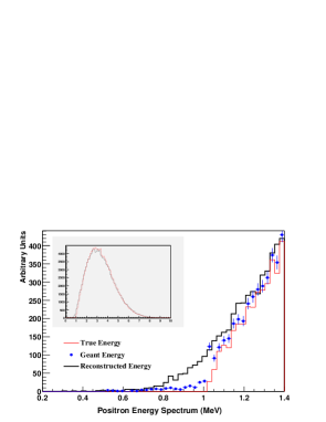
Figure 3.2: Energy spectra associated with the positron’s true energy, simulated energy (Geant Energy), and reconstructed energy at 1 MeV. The full spectrum is shown in the inset, where the red line corresponds to the true energy and the black one corresponds to the reconstructed energy.

For this simulation, 200 PMTs are used to measure the energy deposited in a 20-ton module. The energy resolution is $\sim$15% at 1 MeV. The inefficiencies are 0.32%, 0.37%, and 0.43% for cuts at 0.98 MeV, 1.0 MeV, and 1.02 MeV, respectively. Assuming the energy scale uncertainty is 2% at 1 MeV, this inefficiency variation will produce a 0.05% uncertainty in the detected antineutrino rate. The upper energy requirement for the positron signal will be $E<8$ MeV and will also contribute a negligible uncertainty to the positron detection efficiency.

3.2.4 Neutron Detection Efficiency

The delayed neutron from the inverse beta decay reaction is produced with $\sim$10 keV of kinetic energy. The neutron loses energy in the first few interactions with H and C in the scintillator, and reaches thermal energy in a few microseconds. The neutrons can capture on either H or Gd during or after the thermalization process. We will detect the neutrons that capture on Gd, yielding at least 6 MeV of visible energy from the resulting capture $\gamma$ rays, during the time period 0.3$<T<$200 $\mu$s.

The efficiency for detecting the neutron is given by

$$\epsilon_{n}=P_{Gd}\epsilon_{E}\epsilon_{T}$$ (37)

in which $P_{Gd}$ is the probability to capture on Gd (as opposed to H), $\epsilon_{E}$ is the efficiency of the $E>6$ MeV energy cut for Gd capture, and $\epsilon_{T}$ is the efficiency of the delayed time period cut. In order to measure the rates for two detectors (near and far) with a precision to reach $\sin^{2}2\theta_{13}=0.01$ the baseline requirement for the uncertainty on relative neutron detection efficiencies is $0.25\%$. The $\epsilon_{n}$ for neutrons at the center of a detector module can be determined directly by using a tagged neutron source (either ²⁵²Cf, AmBe or both can be used) and counting the number of neutrons using the time and energy cuts after neutron producing event. (Corrections associated with uniformly distributed neutrons are studied with spallation neutrons, as discussed in Section 6.) This will require measurement of order 1 million neutron captures, and would likely require several hours of measurement. This will be established during the initial comprehensive calibration of each detector.

In addition, the individual components $P_{Gd}$, $\epsilon_{E}$, and $\epsilon_{T}$ can be monitored separately as an additional check on the measurement of $\epsilon_{n}$.

H/Gd ratio

Neutrons are thermalized during their first $10~{}\mu$s of existence in the detector central volume. Thus for times longer than $10~{}\mu$s the delayed neutron capture events will exhibit an exponential time constant, $\tau$, related to the average concentration of Gd in the detector module. The rate of capture, $\Gamma\equiv 1/\tau$, is given by:

$$\Gamma=\Gamma_{Gd}+\Gamma_{H}=[n_{Gd}\sigma_{Gd}+n_{H}\sigma_{H}]v\>$$ (38)

where $n_{H(Gd)}$ is the number density of hydrogen (Gd) in the liquid scintillator and $\sigma_{H(Gd)}$ is the neutron capture cross section on hydrogen (Gd) and $v$ is the thermal velocity. The fraction of neutrons that capture on Gd rather than H is then

$$P_{Gd}=\frac{1}{1+\Gamma_{H}/\Gamma_{Gd}}$$ (39)

and we would like to know this relative fraction between different detector modules to $\sim$0.1%. Thus we must measure the time constants $\tau$ for different detector modules to a relative precision of 0.2 $\mu$s. The value of $\tau$ is expected to be about 30 $\mu$s, so we need to measure it to about 0.5% relative precision. Such a measurement requires measuring about 30,000 neutron captures, which can be done in a few minutes with a neutron source. The Chooz experiment measured the (absolute) $\sim$30 $\mu$s capture time to $\pm$0.5 $\mu$s precision.

Measurement of $\tau$ to 0.5% precision will provide a relative value of $P_{Gd}$ to 0.1% uncertainty, which is the baseline and goal value in Table 3.2.

Energy cut efficiency

Another issue is the neutron detection efficiency associated with the signal from capture of neutrons on Gd in the antineutrino detector volume. An energy threshold of about 6 MeV will be employed to select these delayed events, and the efficiency ($\sim$93%) of this criterion may vary between detector modules depending upon the detailed response of the module. However, this can be calibrated through the use of radioactive sources (see Section 6) and spallation neutron captures. The KamLAND detector gain is routinely (every two weeks) monitored with sources, and a relative long-term gain drift of $\sim 1\%$ is readily monitored with a precision of $0.05\%$. Monte Carlo simulations of the Daya Bay detector response for the Gd capture $\gamma$s indicate that 1% energy scale uncertainty will lead to 0.2% uncertainty in $\epsilon_{E}$, and we use this value as the baseline systematic uncertainty.

We have also performed detailed Monte Carlo simulations of the detector response to neutron sources and spallation neutrons. The results of these studies indicate that we can indeed establish the relative value of $\epsilon_{E}$ to $0.1\%$, even for reasonable variations of detector properties (such as scintillator attenuation length). As an example, Fig. 3.3 shows how the source data can be used with uniform spallation neutrons to bootstrap a non-linear energy scale that corrects the spectrum, independent of attenuation length over the extreme range of 4.5–18 m.

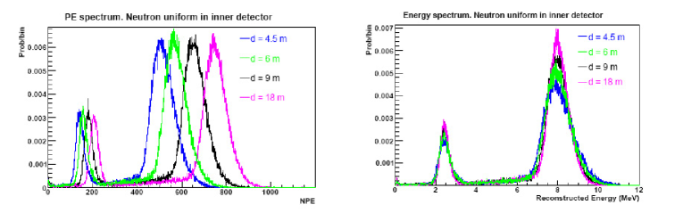
Figure 3.3: Spallation neutron response for detector modules with scintillator optical attenuation lengths of $4.5\leq d\leq 18$ m. The left panel shows the raw photoelectron spectra, whereas the right panel shows the spectra rescaled according to a non-linear rescaling procedure we have developed. The rescaled 6 MeV effective energy threshold produces a constant value of $\epsilon_{E}=93\%$ to within 0.4% over this extreme range of attenuation length.

Therefore, we estimate a value of 0.1% for the goal systematic uncertainty in $\epsilon_{E}$.

Time cuts

The time correlation of the prompt (positron) event and the delayed (neutron) event is a critical aspect of the event signature. Matching the time delays of the start and end times of this time window between detector modules is crucial to reducing systematic uncertainties associated with this aspect of the antineutrino signal. If the starting time ($\sim$0.3 $\mu$s) and ending time ($\sim$200 $\mu$s) of the delayed event window is determined to $\sim$10 ns precision, the resulting uncertainty associated with missed events is $\sim$0.03%. We will insure that this timing is equivalent for different detector modules by slaving all detector electronics to one master clock. We estimate that with due care, the relative neutron efficiency for different modules due to timing is known to $\sim$0.03%, and we use this value as the estimated goal systematic uncertainty. We use a more conservative 0.1% value for the baseline value.

3.2.5 Neutron Multiplicity

Chooz required a cut on the neutron multiplicity to eliminate events where it appeared that there were two neutron captures following the positron signal, resulting in a 2.6% inefficiency and associated 0.5% systematic uncertainty. These multiple neutron events are due to muon-induced spallation neutrons, and will be reduced to a much lower level by the increased overburden available at the Daya Bay site. For the near site at 500 m baseline, the muon rate relative to the signal rate will be more than a factor nine lower than for the Chooz site. Therefore, events with multiple neutron signals will be reduced by this factor relative to Chooz, and should present a much smaller problem for the Daya Bay site. We therefore estimate a 0.05% value for this systematic uncertainty and use this for both the baseline and goal values.

3.2.6 Trigger

The trigger efficiency can be measured to high precision (0.01%) using studies with pulsed light sources in the detector. (We note that KamLAND has used this method to determine 99.8% absolute trigger efficiency [4].) In addition, we will employ several redundant triggers so that they can be used to cross-check each other to high precision. We estimate a systematic uncertainty of 0.01% can be achieved, and use this for both the baseline and goal values.

3.2.7 Live Time

The detector live time can be measured accurately by counting a 100 MHz clock using the detector electronics, and normalizing to the number of clock ticks in a second (as defined by a GPS receiver signal). The uncertainty associated with this procedure should be extremely small, and certainly negligible relative to the other systematic uncertainties. For example, SNO measured the relative live times for their day/night analysis with a relative fractional uncertainty of $5\times 10^{-7}$.

3.3 Cross-calibration and Swapping of Detectors

3.3.1 Detector Swapping

The connection of the two near detector halls and the far hall by horizontal tunnels provides the Daya Bay experiment with the unique and important option of swapping the detectors between the locations. This could enable the further reduction of detector-related systematic uncertainties in the measurement of the ratio of neutrino fluxes at the near and far locations. Although the estimated baseline and goal systematic uncertainties in Table 3.2 are sufficient to achieve a sensitivity of 0.01 in $\sin^{2}2\theta_{13}$, implementation of detector swapping could provide an important method to further reduce systematic uncertainties and increase confidence in the experimental results.

The swapping concept is easy to demonstrate for a simple scenario with a single neutrino source and only two detectors deployed at two locations, near and far. The desired measurement is the ratio of event rates at the near and far locations: $N/F$. With detector #1 (efficiency $\epsilon_{1}$) at the near location and detector #2 (efficiency $\epsilon_{2}$)at the far location we would measure

$$\frac{N_{1}}{F_{2}}=\left(\frac{\epsilon_{1}}{\epsilon_{2}}\right)\frac{N}{F}\>$$ (40)

By swapping the two detectors and making another measurement, we can measure

$$\frac{N_{2}}{F_{1}}=\left(\frac{\epsilon_{2}}{\epsilon_{1}}\right)\frac{N}{F}\>$$ (41)

where we have assumed that the detector properties (e.g., efficiencies) do not change when the detector is relocated. We can now combine these two measurements to obtain a value of $N/F$ that is, to first order, independent of the detector efficiencies:

$$\frac{1}{2}\left(\frac{N_{1}}{F_{2}}+\frac{N_{2}}{F_{1}}\right)=\frac{N}{F}\left(1+\frac{\delta^{2}}{2}\right)$$ (42)

where we have defined

$$\delta\equiv\frac{\epsilon_{2}}{\epsilon_{1}}-1\>$$ (43)

Note that even if the detector efficiencies are different by as much as 1%, we can determine $N/F$ to a fractional precision better than $10^{-4}$.

The layout of the Daya Bay experiment involves two near sites with two detectors each, and a far site with four detectors. The simplest plan is to designate the eight detectors as four pairs: (1,2), (3,4), (5,6), (7,8). Using four running periods (designated I, II, III, IV, separated by three detector swaps) we can arrange for each detector to be located at the far site half the time and a near site half the time by swapping two pairs between running periods, as shown in Table 3.3.

Run Period	Near(DB)	Near(LA)	Far
I	1,3	5,7	2,4,6,8
II	2,3	6,7	1,4,5,8
III	2,4	6,8	1,3,5,7
IV	1,4	5,8	2,3,6,7

Table 3.3: Swapping scheme with four running periods. The detectors (labelled 1–8) are deployed at the Near(DB), Near(LA), and Far sites during each period as indicated in this table.

Ratios of event rates can be combined in a fashion analogous to the above discussion to provide cancellation of detector-related systematic uncertainties and also reactor power systematic uncertainties. Careful calibration of the detectors following each swap will be necessary to insure that each detector’s performance does not change significantly due to relocation. In particular, all the parameters in Table 3.2 need to be checked and, if necessary, corrections applied to restore the detection efficiency to the required precision through, e.g., changes in calibration constants.

Successful implementation of this swapping concept will lead to substantial reduction in many of the detector-related systematic uncertainties. The uncertainty associated with the H/C and H/Gd ratios should be completely eliminated. By measuring the fluid levels before and after swapping, we can insure that the detector volume will be the same with negligible uncertainty. However, due to the residual uncertainty in the monitored temperature of the detector module ($0.1^{\circ}$ C), there will be a residual uncertainty in the detector mass of 0.006%, and this is the value quoted in Table 3.2.

3.3.2 Detector Cross-calibration

Another important feature of the design of the Daya Bay experiment is the presence of two detector modules at each near site. During a single running period (I, II, III, or IV) each near detector module will measure the neutrino rate with 0.23% statistical precision. If the systematic uncertainties are smaller than this, the two detectors at the near site should measure the same rate, giving a detector asymmetry of $0\pm 0.34$% (statistical uncertainty only). Combining all the detector pairs in all 4 running periods will yield an asymmetry of $0\pm 0.04$% (statistical uncertainty only). These asymmetries are an important check to ensure that the detector-related systematic uncertainties are under control. In addition, this analysis can provide information on the the degree to which the detector-related systematic uncertainties are correlated or uncorrelated so that we know how to handle them in the full analysis including the far site.

Finally, the near detector data can provide important information on the reactor power measurements. We will measure the ratio

$$R_{\rm near}=\frac{S_{DB}}{S_{LA}}$$ (44)

where $S_{DB}$ ($S_{LA}$) is the detector signal (background subtracted, normalized to the reactor power) for the Daya Bay (Ling Ao) near site. If the reactor powers are correct (and the detector systematic uncertainties are under control) then we expect $R_{\rm near}=1.0\pm 0.24\%\pm 0.51\%$, where the first uncertainty is statistical (only 1 of the 4 running periods) and the second uncertainty is the detector (baseline) systematic uncertainty. Note that these uncertainties are small relative to the expected 2% uncorrelated reactor power uncertainty, so measurement of $R_{\rm near}$ will provide an important check (and even perhaps additional information) on the reactor powers. Furthermore, studies of the measured neutrino spectra in the different near detectors during different parts of the reactor fuel cycle can help provide constraints on the fuel cycle effects on the spectrum.

3.4 Backgrounds

In the Daya Bay experiment, the signal events (inverse beta decay reactions) have a distinct signature of two time-ordered signals: a prompt positron signal followed by a delayed neutron-capture signal. Backgrounds can be classified into two categories: correlated and uncorrelated backgrounds. If a background event is triggered by two signals that come from the same source, such as those induced by the same cosmic muon, it is a correlated background event. On the other hand, if the two signals come from different sources but satisfy the trigger requirements by chance, the event is an uncorrelated background.

There are three important sources of backgrounds in the Daya Bay experiment: fast neutrons, ⁸He/ ⁹Li, and natural radioactivity. A fast neutron produced by a cosmic muon in the surrounding rock or the detector can produce a signal mimicking the inverse beta decay reaction in the detector: the recoil proton generates the prompt signal and the capture of the thermalized neutron provides the delayed signal. The ⁸He/ ⁹Li isotopes produced by cosmic muons have substantial beta-neutron decay branching fractions, 16% for ⁸He and 49.5% for ⁹Li. The beta energy of the beta-neutron cascade overlaps the positron signal of neutrino events, simulating the prompt signal, and the neutron emission forms the delayed signal. Fast neutrons and ⁸He/ ⁹Li isotopes create correlated backgrounds since both the prompt and delayed signals are from the same single parent muon. Some neutrons produced by cosmic muons are captured in the detector without proton recoil energy. A single neutron capture signal has some probability to fall accidentally within the time window of a preceding signal due to natural radioactivity in the detector, producing an accidental background. In this case, the prompt and delayed signals are from different sources, forming an uncorrelated background.

All three major backgrounds are related to cosmic muons. Locating the detectors at sites with adequate overburden is the only way to reduce the muon flux and the associated background to a tolerable level. The overburden requirements for the near and far sites are quite different because the signal rates differ by more than a factor of 10. Supplemented with a good muon identifier outside the detector, we can tag the muons going through or near the detector modules and reject backgrounds efficiently.

In this section, we describe our background studies and our strategies for background management. We conclude that the background-to-signal ratio will be around 0.3% at the near sites and around 0.2% at the far site, and that the major sources of background can be quantitatively studied in-situ.

3.4.1 Cosmic Muons in the Underground Laboratories

The most effective and reliable approach to minimize the backgrounds in the Daya Bay experiment is to have sufficient amount of overburden over the detectors. The Daya Bay site is particularly attractive because it is located next to a 700-m high mountain. The overburden is a major factor in determining the optimal detector sites. The location of detector sites has been optimized by using a global $\chi^{2}$ analysis described in Section 3.5.1.

Detailed simulation of the cosmogenic background requires accurate information of the mountain profile and rock composition. Figure 3.4 shows the mountain profile converted from a digitized 1:5000 topographic map.

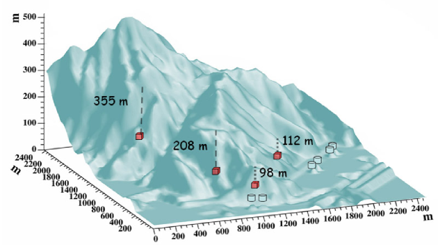
Figure 3.4: Three dimensional profile of Pai Ya Mountain, where the Daya Bay experimental halls will be located, generated from a 1:5000 topographic map of the Daya Bay area.

The horizontal tunnel and detector sites are designed to be about $-$20 m PRD. Several rock samples at different locations of the Daya Bay site were analyzed by two independent groups. The measured rock density ranges from 2.58 to 2.68 g/cm³. We assume an uniform rock density of 2.60 g/cm³ in the present background simulation. A detailed description of the topography and geology of the Daya Bay area is given in Chapter 4.

The standard Gaisser formula [5] is known to poorly describe the muon flux at large zenith angle and at low energies. This is relevant for the Daya Bay experiment since the overburden at the near sites is only $\sim$100 m. We modified the Gaisser formula as

$$\frac{dI}{dE_{\mu}d\cos\theta}=0.14\left(\frac{E_{\mu}}{\rm GeV}\left(1+\frac{3.64{\rm\,GeV}}{E_{\mu}(\cos\theta^{\ast})^{1.29}}\right)\right)^{-2.7}\left[\frac{1}{1+\frac{1.1E_{\mu}\cos\theta^{\ast}}{115{\rm\,GeV}}}+\frac{0.054}{1+\frac{1.1E_{\mu}\cos\theta^{\ast}}{850{\rm\,GeV}}}\right]$$ (45)

which is the same as the standard formula, except that the polar angle $\theta$ is substituted with $\theta^{\ast}$,

$$\cos\theta^{\ast}=\sqrt{\frac{(\cos\theta)^{2}+P_{1}^{2}+P_{2}(\cos\theta)^{P_{3}}+P_{4}(\cos\theta)^{P_{5}}}{1+P_{1}^{2}+P_{2}+P_{4}}}$$ (46)

as defined in [6]. The parameters are determined to be $P_{1}=0.102573,\;P_{2}=-0.068287,\;P_{3}=0.958633,\;P_{4}=0.0407253$, and $P_{5}=0.817285$, by using CORSIKA to simulate the muon production in the atmosphere. The comparison of the modified formula with data is shown in Fig. 3.6, where the calculations with the standard Gaisser formula are also shown.

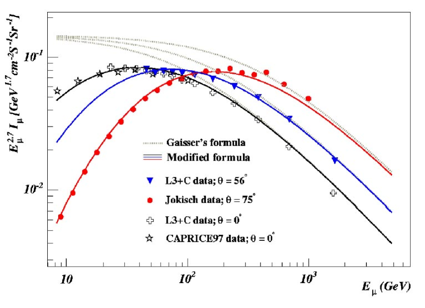
Figure 3.5: Comparison of the modified formula (solid lines) with data. Calculations with the standard Gaisser’s formula are shown in dashed lines. The data are taken from Ref. [7, 8].

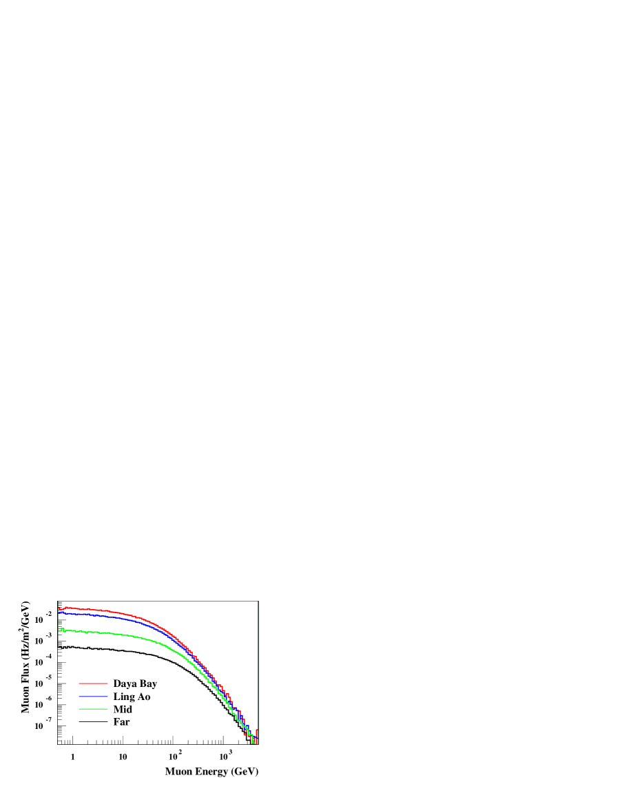
Figure 3.6: Muon flux as a function of the energy of the surviving muons. The four curves from upper to lower correspond to the Daya Bay near site, the Ling Ao near site, the mid site and the far site, respectively.

At muon energies of several tens of GeV, the standard Gaisser formula has large discrepancies with data while the modified formula agrees with data in the whole energy range.

Using the mountain profile data, the cosmic muons are transported from the atmosphere to the underground detector sites using the MUSIC package [9]. Simulation results are shown in Table 3.4 for the optimal detector sites.

	DYB site	LA site	Mid site	Far site
Vertical overburden (m)	98	112	208	355
Muon Flux (Hz/m2)	1.16	0.73	0.17	0.041
Muon Mean Energy (GeV)	55	60	97	138

Table 3.4: Vertical overburden of the detector sites and the corresponding muon flux and mean energy.

The muon energy spectra at the detector sites are shown in Fig. 3.6. The four curves from upper to lower corresponds to the Daya Bay near site, the Ling Ao near site, the mid site and the far site, respectively.

3.4.2 Simulation of Neutron Backgrounds

The neutron production rates will depend upon the cosmic muon flux and average energy at the detector. However, the neutron backgrounds in the detector also depend on the local detector shielding. The neutrino detectors will be shielded by at least 2.5 meters of water. This water buffer will be used as a Cherenkov detector to detect muons. Thus neutrons produced by muons in the detector module or the water buffer will be identified by the muon signal in the water Cherenkov detector. In addition, neutrons created by muons in the surrounding rock will be effectively attenuated by the 2.5 m water buffer. Together with another muon tracker outside the water buffer, the combined muon tag efficiency is designed to be 99.5%, with an uncertainty smaller than 0.25%.

From the detailed muon flux and mean energy at each detector site, the neutron yield, energy spectrum, and angular distribution can be estimated with an empirical formula [10] which has been tested against experimental data whenever available. A full Monte Carlo simulation has been carried out to propagate the primary neutrons produced by muons in the surrounding rocks, the water buffer, and the oil buffer layer of the neutrino detector, to the detector. The primary neutrons are associated with their parent muons in the simulation so that we know if they can be tagged by the muon detector. Neutrons produced by muons that pass through the liquid scintillator neutrino detector will be tagged with 100% efficiency. Neutrons produced in the water buffer will be tagged with an efficiency of 99.5%, since their parent muons must pass through the muon systems. Neutrons produced in the rocks, however, have to traverse at least 2.5 meters of water to reach a detector module. About 70% of the neutrons that enter the detector modules from the surrounding rock arise from parent muons that leave a signal in the muon system (i.e., “tagged”). About 30% of the neutrons that enter the detector modules from the surrounding rocks arise from muons that miss the muon system ($\equiv$ “untagged”). The neutron background after muon rejection is the sum of the untagged events and 0.5% (due to veto inefficiency) of the tagged events.

Some energetic neutrons will produce tertiary particles, including neutrons. For those events that have energy deposited in the liquid scintillator, many have a complex time structure due to multiple neutron scattering and captures. These events are split into sub-events in 50 ns time bins. We are interested in two kinds of events. The first kind has two sub-events. The first sub-event has deposited energy in the range of 1 to 8 MeV, followed by a sub-event with deposited energy in the range of 6 to 12 MeV in a time window of 1 to 200 $\mu$s. These events, called fast neutron events, can mimic the antineutrino signal as correlated backgrounds. The energy spectrum of the prompt signal of the fast neutron events, e.g. at the far site, is shown in Fig. 3.7 up to 50 MeV.

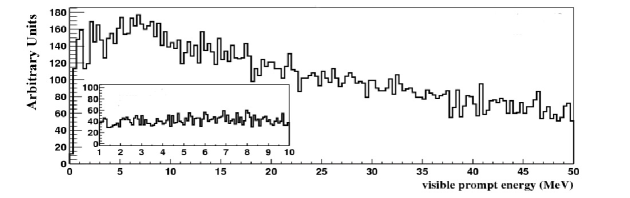
Figure 3.7: The prompt energy spectrum of fast neutron background at the Daya Bay far detector. The inset is an expanded view of the spectrum from 1 to 10 MeV.

The other kind of events has only one sub-event with deposited energy in range of 6 to 12 MeV. These events, when combined with the natural radioactivity events, can provide the delayed signal to form the uncorrelated backgrounds. We call them single neutron events. Most of the single neutron events are real thermalized neutrons while others are recoil protons that fall into the 6–12 MeV energy range accidentally. About 1.5% thermalized neutrons will survive the 200 $\mu$s cut, even though its parent muon is tagged. This inefficiency will be also taken into account when calculating the single neutron rate. The neutron simulation results are listed in Table 3.5.

		DYB site	LA site	far site
fast neutron	tagged	19.6	13.1	2.0
(/day/module)	untagged	0.5	0.35	0.03
single neutron	tagged	476	320	45
(/day/module)	untagged	8.5	5.7	0.63

Table 3.5: Neutron rates in a 20-ton module at the Daya Bay sites. The rows labelled ”tagged” refer to the case where the parent muon track traversed and was detected by the muon detectors, and thus it could be tagged. Rows labelled ”untagged” refer to the case where the muon track was not identified by the muon detectors.

The rate and energy spectrum of the fast neutron backgrounds can be studied with the tagged sample.

3.4.3 Cosmogenic Isotopes

Cosmic muons, even if they are tagged by the muon identifier, can produce radioactive isotopes in the detector scintillator which decay by emitting both a beta and a neutron ($\beta$-neutron emission isotopes). Some of these so-called cosmogenic radioactive isotopes live long enough such that their decay cannot be reliably associated with the last tagged muon. Among them, ⁸He and ⁹Li with half-lives of 0.12 s and 0.18 s, respectively, constitute the most serious correlated background sources. The production cross section of these two isotopes has been measured with muons at an energy of 190 GeV at CERN [11]. Their combined cross section is $\sigma(^{9}{\rm Li}+^{8}{\rm He})=(2.12\pm 0.35)~{}\mu{\rm barn}$. Since their lifetimes are so close, it is hard to extract individual cross sections. About 16% of ⁸He and 49.5% of ⁹Li will decay by $\beta$-neutron emission. Using the muon flux and mean energy at each detector site (from Section 3.4.1) and an energy dependent cross section, $\sigma_{\rm tot}(E_{\mu})\propto E_{\mu}^{\alpha}$, with $\alpha=0.73$, the estimated ⁸He+⁹Li backgrounds are listed in Table 3.6.

	DYB site	LA site	Far site
(8He+9Li)/day/module	3.7	2.5	0.26

Table 3.6: ⁸He+⁹Li rates in a 20-ton module at the Daya Bay sites.

The recent Double Chooz paper [13] includes new reactor-off data from Chooz [1] that allow a better separation of ⁹Li from fast neutron background. This basically comes from including previously unreleased high energy data in the fit. The extracted ⁹Li background level was 0.7$\pm$0.2 events/day. The mean muon energy in Chooz was $\sim$ 60 GeV, almost the same as the Daya Bay near site (55 GeV) and the Ling Ao near site (60 GeV). The fitting is based on the assumption that the fast neutron background is flat in energy spectrum. Scaling from the Chooz result, the Daya Bay experiment will have 8.0, 5.4, and 0.57 ⁹Li events per module per day at the Daya Bay near site, the Ling Ao near site, and the far site, respectively. These estimates are twice as large as the estimates from the CERN cross section.

The KamLAND experiment measures this ⁹Li/ ⁸He background very well by fitting the time interval since last muon. The muon rate is 0.3 Hz in the active volume of KamLAND detector. The mean time interval of successive muons is $\sim 3$ seconds, much longer than the lifetimes of ⁹Li/ ⁸He. For the Daya Bay experiment, the target volume of a 20 ton detector module has a cross section around 10 m², thus the muon rate is around 10 Hz at the near sites, resulting in a mean time interval of successive muons shorter than the lifetimes of ⁹Li/⁸He. With a modified fitting algorithm, we find that it is still feasible to measure the isotope background in-situ.

From the decay time and $\beta$-energy spectra fit, the contribution of ⁸He relative to that of ⁹Li was determined by KamLAND to be less than 15% at 90% confidence level [14]. Furthermore, the ⁸He contribution can be identified by tagging the double cascade ⁸He $\rightarrow^{8}$Li $\rightarrow^{8}$Be. So we assume that all isotope backgrounds are ⁹Li. They can be determined with a maximum likelihood fitting even at 10 Hz muon rate, by taking all contributions from the preceding muons into account. The resolution of the background-to-signal ratio can be determined to be [15]

$$\sigma_{b}=\frac{1}{\sqrt{N}}\cdot\sqrt{(1+\tau R_{\mu})^{2}-1}\,$$ (47)

where $N$ is the total number of neutrino candidates, $\tau$ is the lifetime of ⁹Li, and $R_{\mu}$ is the muon rate in the target volume of detector. The resolution is insensitive to the ⁹Li level since the statistical fluctuation of neutrino events dominates the uncertainty. The background-to-signal ratio of ⁹Li background can be measured to $\sim$ 0.3% with two 20-ton modules at the near sites of the Daya Bay experiment and $\sim$ 0.1% at the far site with four 20-ton modules, with the data sample of three years of running. The fitting uses time information only. Inclusion of energy and vertex information could further improve the precision.

A Monte Carlo has been carried out to check the fitting algorithm. The background-to-signal ratio is fixed at 1%. The total number of neutrino candidates is $2.5\times 10^{5}$, corresponding to the far site statistical uncertainty, 0.2%. Figure 3.9 shows the fitting results as a function of muon rate.

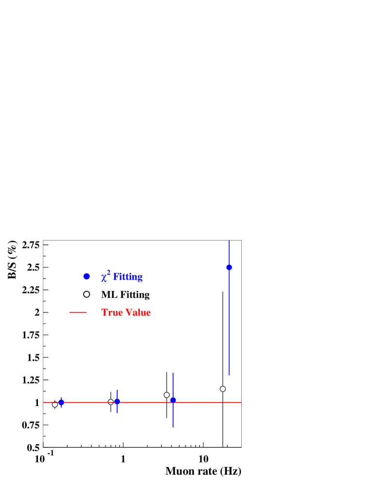
Figure 3.8: Fitting results as a function of the muon rate. The uncertainty bars show the precision of the fitting. The $\chi^{2}$ fitting uses the same muon rate as the maximum likelihood fitting and is shown to the right of it.

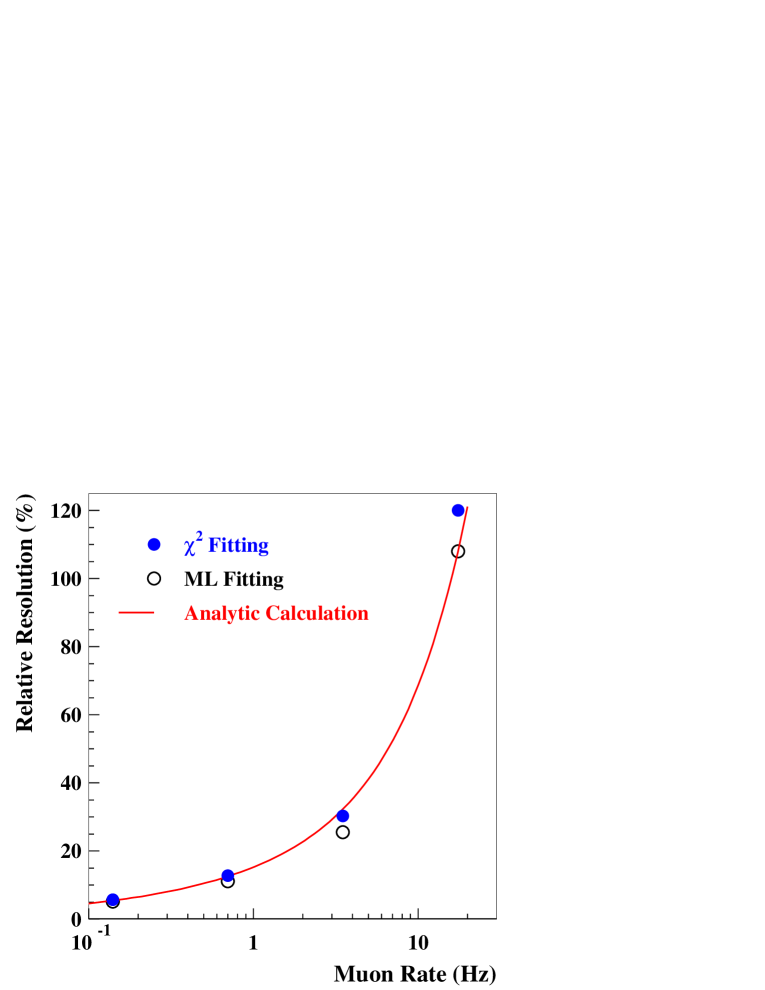
Figure 3.9: The fitting precision as a function of the muon rate, comparing with the analytic estimation of Eq. 47. The y-axis shows the relative resolution of the background-to-signal ratio.

The data sample generation and fitting were performed 400 times for each point to get the fitting precision. In Fig. 3.9 the fitting precision is compared to the analytic formula Eq. 47 with the same Monte Carlo samples. The Monte Carlo results for minimizing $\chi^{2}$, the maximum likelihood fit, and the simple analytical estimation are in excellent agreement.

KamLAND also found that most ⁸He/ ⁹Li background are produced by showering muons [14]. A 2-second veto of the whole detector is applied at KamLAND to reject these backgrounds. Roughly 3% of cosmic muons shower in the detector. It is not feasible for Daya Bay to apply a 2-second veto since the dead time of the near detector would be more than 50%. However, if the Daya Bay detector is vetoed for 0.5 s after a showering muon, about 85% of the ⁸He/ ⁹Li backgrounds caused by shower muons can be rejected. Approximately 30% of the ⁸He/ ⁹Li background will remain: $\sim 15\%$ from non-showering muons and $\sim 15\%$ from showering muons. Although additional uncertainties may be introduced due to the uncertainties in the relative contributions from showering and non-showering muons and the uncertainties arising from the additional cuts (e.g., increased dead time), this rejection method can cross check the fitting method and firmly determine the background-to-signal ratio to 0.3% at the near sites and to 0.1% at the far site.

Some other long-lived cosmogenic isotopes, such as ¹²B/¹²N, beta decay without an accompanying neutron. They can not form backgrounds themselves but can fake the delayed ‘neutron’ signal of an accidental background if they have beta decay energy in the 6–10 MeV range. The expected rates from these decays in the antineutrino detector are listed in Table 3.7. The ¹²B/¹²N cross section is taken from KamLAND [14] and the others are taken from measurement at CERN [11]. They are extrapolated to Daya Bay mean muon energies using the power law $\sigma_{\rm tot}(E_{\mu})\propto E_{\mu}^{0.73}$. The total rates of all these isotopes of visible energy in detector in the 6–10 MeV range, where they can be misidentified as a neutron capture signal on Gadolinium, are 210, 141, and 14.6 events per module per day at the Daya Bay near site, the Ling Ao near site, and the far site, respectively. The dominant contribution is from ¹²B/¹²N. KamLAND found that ¹²N yield is smaller than 1% of ¹²B. Since the half-life of ¹²B is short comparing to the mean muon interval, the rate can be well determined in situ by fitting the time since last muon. Using Eq. 47, the yield can be determined to a precision of 0.34, 0.25, and 0.015 events per module per day at the Daya Bay near site, the Ling Ao near site, and the far site, respectively, using three years’ data sample. Therefore, we expect those isotopes will introduce very little uncertainties in the background subtraction. On the other side, these isotopes, uniformly produced inside the detector, can be used to monitor detector response.

isotopes	$E_{\rm max}$	$T_{1/2}$(s)	DYB site	LA site	far site
	(MeV)	(s)	(/day/module)	(/day/module)	(/day/module)
12B/12N	13.4 ($\beta^{-}$)	0.02/0.01	396	267	27.5
9C	16.0 ($\beta^{+}$)	0.13	16.6	11.2	1.15
8B	13.7 ($\beta^{+}$)	0.77	24.5	16.5	1.71
8Li	16.0 ($\beta^{-}$)	0.84	13.9	9.3	0.96
11Be	11.5 ($\beta^{-}$)	13.8	$<$8.0	$<$5.4	$<$0.56
Total in 6-10 MeV			210	141	14.6

Table 3.7: Cosmogenic radioactive isotopes without neutron emission but with beta decay energy greater than 6 MeV. Cross sections are taken from KamLAND [14] (¹²B/¹²N) and Hagner [11] (others).

3.4.4 Radioactivity

Natural radioactivity and the single neutron events induced by cosmic muons may occur within a given time window accidentally to form an uncorrelated background. The coincidence rate is given by $R_{\gamma}R_{n}\tau,$ where $R_{\gamma}$ is the rate of natural radioactivity events, $R_{n}$ is the rate of spallation neutron, and $\tau$ is the length of the time window. With the single neutron event rate given in the previous section, the radioactivity should be controlled to 50 Hz to limit the accidental backgrounds $<0.1$%. The accidental backgrounds can be well determined in-situ by measurement of the individual singles rates from radioactivity and the single neutrons. The energy spectrum can be also well determined.

Past experiments suppressed uncorrelated backgrounds with a combination of carefully selected construction materials, self-shielding, and absorbers with large neutron capture cross section. However, additional care is necessary to lower the detector energy threshold much below 1 MeV. A higher threshold will introduce a systematic uncertainty in the efficiency of detecting the positron. In the following, the singles rate is from radioactivity depositing $>$1 MeV of visible energy in detector.

Radioactive background can come from a variety of sources. For simplicity, U, Th, K, Co, Rn, Kr in the following text always mean their radioactive isotopes ²³⁸U, ²³²Th, ⁴⁰K, ⁶⁰Co, ²²²Rn, ⁸⁵Kr. The radioactive sources include

• U/Th/K in the rocks around the detector hall.

• U/Th/K in the water buffer.

• Co in the detector vessel and other supporting structures.

• U/Th/K in weld rods.

• U/Th/K in the PMT glass.

• U/Th/K in the scintillator.

• U/Th/K in materials used in the detector.

• Dust and other impurities

• Rn and Kr in air.

• Cosmogenic isotopes.

The radioactivity of rock samples from the Daya Bay site has been measured by several independent groups, including the Institute for Geology and Geophysics (IGG). The concentrations are: $\sim$10 ppm for U, $\sim$30 ppm for Th, and $\sim$5 ppm for K. The effect of the rock radioactivity on the antineutrino detectors has been studied with Monte Carlo. With the shielding of 2.5-meter water buffer and 45 cm oil buffer, there are 0.65 Hz, 2.6 Hz, and 0.26 Hz singles rates with visible energy greater than 1 MeV in each antineutrino detector module for U/Th/K, respectively. The total rate is $\sim$3.5 Hz.

The geological environment and rock composition are very similar in Hong Kong and Daya Bay. The spectrum of natural radioactivity that we have measured of the rock in the Aberdeen Tunnel in Hong Kong is shown in Fig. 3.10.

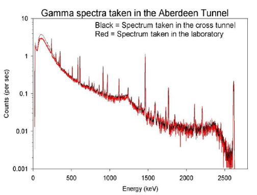
Figure 3.10: Spectrum of natural radioactivity measured with a Ge crystal in the Hong Kong Aberdeen Tunnel. Prominent peaks for ⁴⁰K (1.461 MeV) and ²⁰⁸Tl (2.615 MeV) are clearly evident along with many other lines associated with the U/Th series.

The water buffer will be circulated and purified to achieve a long attenuation length for Cherenkov light as well as low radioactivity. Normally tap water has 1 ppb U, 1 ppb Th, and also 1 ppb K. If filling with tap water, the water buffer will contribute 1.8 Hz, 0.4 Hz, and 6.3 Hz singles rates from U/Th/K, respectively. Purified water in the water pool will have much lower radioactivity. Thus the radioactivity from water buffer can be ignored.

The Co in stainless steel varies from batch to batch and should be measured before use as detector material, such as the outer vessel. U/Th/K concentration in normal weld rods are very high. There are non-radioactivity weld rods commercially available. Weld rods TIG308 used in KamLAND were measured to have $<$1 ppb Th, $0.2\pm 0.08$ ppb U, $0.1\pm 0.03$ ppb K, and $2.5\pm 0.04$ mBq/kg Co, five orders of magnitude lower than normal weld rods. The welded stainless steel in KamLAND has an average radioactivity of 3 ppb Th, 2 ppb U, 0.2 ppb K, and 15 mBq/kg Co. Assuming the same radioactivity for the vessel of the Daya Bay neutrino detector module, the corresponding rate from a 20-ton welded stainless steel vessel are 7 Hz, 4.6 Hz, 1.5 Hz, 4.5 Hz for U/Th/K/Co, respectively for a total of 17.6 Hz.

A potential PMT candidate is the Hamamatsu R5912 with low radioactivity glass. The concentrations of U and Th are both less than 40 ppb in the glass, and that of K is 25 ppb. The Monte Carlo study shows that the singles rate is 2.2 Hz, 1 Hz, 4.5 Hz for U/Th/K, respectively, with a 20 cm oil buffer from the PMT surface to the liquid scintillator. The total rate from the PMT glass is 7.7 Hz.

Following the design experience of Borexino and Chooz, backgrounds from impurities in the liquid scintillator can be reduced to the required levels. A major source is the U/Th contamination in the Gadolinium, which can be purified before doped into liquid scintillator. The U/Th/K concentration of $10^{-12}g/g$ in liquid scintillator will contribute only 0.8 Hz of background in a 20-ton detector module.

Radon is one of the radioactive daughters of ²³⁸U, which can increase the background rate of the experiment. The Radon concentration in the experimental halls can be kept to an acceptable level by ventilation with fresh air from outside. Since the neutrino detector modules are immersed in a 2.5-meter thick water buffer, it is expected that the radon contribution, as well as the krypton, can be safely ignored for the water pool design.

The $\beta$ decay of long lived radioactive isotopes produced by cosmic muons in the scintillator will contribute a couple of Hz at the near detector, and less than 0.1 Hz at the far detector. The rate of muon decay or muon capture are 2–6% of the muon rate. So they can be ignored when viewed as a source of singles.

3.4.5 Background Subtraction Uncertainty

There are other sources of backgrounds, such as cosmogenic nuclei, stopped-muon decay, and muon capture. While they are important for a shallow site, our study shows that they can be safely ignored at Daya Bay.

Assuming a muon efficiency of 99.5%, the three major backgrounds are summarized in Table 3.8 while the other sources are negligible (the signal and singles rates are also included).

	DYB site	LA site	far site
Antineutrino rate (/day/module)	930	760	90
Natural radiation (Hz)	$<$50	$<$50	$<$50
Single neutron (/day/module)	18	12	1.5
$\beta$-emission isotopes	210	141	14.6
Accidental/Signal	$<$0.2%	$<$0.2%	$<$0.1%
Fast neutron/Signal	0.1%	0.1%	0.1%
8He9Li/Signal	0.3%	0.2%	0.2%

Table 3.8: Summary of signal and background rates in the antineutrino detectors at Daya Bay. A neutron detection efficiency of 78% has been applied to the antineutrino and single-neutron rates.

In our sensitivity study, the uncertainties were taken to be 100% for the accidental and fast neutron backgrounds. The ⁸He/ ⁹Li background can be measured to an uncertainty of 0.3% and 0.1% at the near and far sites, respectively.

The rates and energy spectra of all three major backgrounds can be measured in-situ. Thus the backgrounds at the Daya Bay experiment are well controlled. The simulated energy spectra of backgrounds are shown in Fig. 3.11. The background-to-signal ratios are taken at the far site.

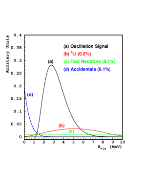
Figure 3.11: Spectra of three major backgrounds for the Daya Bay experiment and their size relative to the oscillation signal, which is the difference of the expected neutrino signal without oscillation and the ‘observed’ signal with oscillation for $\sin^{2}2\theta_{13}=0.01$.

3.5 Sensitivity

If $\theta_{13}$ is non-zero, a relative rate deficit will be present at the far detector due to oscillation. At the same time, the energy spectra of neutrino events at the near and far detectors will be different because neutrinos of different energies oscillate at different frequencies. Both the rate deficit and spectral distortion of neutrino signal will be exploited in the final analysis to obtain maximum sensitivity. When the neutrino event statistics are low ($<$400 ton$\cdot$GW$\cdot$y), the sensitivity is dominated by the rate deficit. For luminosity higher than 8000 ton$\cdot$GW$\cdot$y, the sensitivity is dominated by the spectral distortion [16]. The Daya Bay experiment will have $\sim$4000 ton$\cdot$GW$\cdot$y exposure in three years, so both rate deficit and shape distortion effects will be important to the analysis.

3.5.1 Global $\chi^{2}$ Analysis

Many systematic uncertainties will contribute to the final sensitivity of the Daya Bay experiment, and many of them are correlated. The correlation of the uncertainties must be taken into account correctly. A rigorous analysis of systematic uncertainties can be done by constructing a $\chi^{2}$ function with pull terms, where the uncertainty correlations can be introduced naturally [16, 17, 18, 19]:

$$\chi^{2} = \min_{\gamma}\sum_{A=1}^{8}\sum_{i=1}^{N_{bins}}\frac{\left[M_{i}^{A}-T_{i}^{A}\left(1+\alpha_{c}+\sum_{r}\omega_{r}^{A}\alpha_{r}+\beta_{i}+\varepsilon_{D}+\varepsilon_{d}^{A}\right)-\eta_{f}^{A}F^{A}_{i}-\eta_{n}^{A}N^{A}_{i}-\eta_{s}^{A}S^{A}_{i}\right]^{2}}{T_{i}^{A}+\sigma_{b2b}^{2}}$$ (48)

$$+ \frac{\alpha_{c}^{2}}{\sigma_{c}^{2}}+\sum_{r}\frac{\alpha_{r}^{2}}{\sigma_{r}^{2}}+\sum_{i=1}^{N_{bins}}\frac{\beta_{i}^{2}}{\sigma_{\rm shp}^{2}}+\frac{\varepsilon_{D}^{2}}{\sigma_{D}^{2}}+\sum_{A=1}^{8}\left[\left(\frac{\varepsilon_{d}^{A}}{\sigma_{d}}\right)^{2}+\left(\frac{\eta_{f}^{A}}{\sigma_{f}^{A}}\right)^{2}+\left(\frac{\eta_{n}^{A}}{\sigma_{n}^{A}}\right)^{2}+\left(\frac{\eta_{s}^{A}}{\sigma_{s}^{A}}\right)^{2}\right]\$$

where $A$ sums over detector modules, $i$ sums over energy bins, and $\gamma$ denotes the set of minimization parameters, $\gamma=\{\alpha_{c},\alpha_{r},\beta_{i},\varepsilon_{D},\varepsilon_{d}^{A},\eta_{f}^{A},\eta_{n}^{A},\eta_{s}^{A}\}$. The $\gamma$’s are used to introduce different sources of systematic uncertainties. The standard deviations of the corresponding parameters are $\{\sigma_{c},\sigma_{r},\sigma_{\rm shp},\sigma_{D},\sigma_{d},\sigma_{f}^{A},\sigma_{n}^{A},\sigma_{s}^{A}\}$. They will be described in the following text. $T_{i}^{A}$ is the expected events in the $i$-th energy bin in detector $A$, and $M_{i}^{A}$ is the corresponding measured events. $F^{A}_{i},N^{A}_{i},S^{A}_{i}$ are number of fast neutron, accidental, and ⁸He/ ⁹Li backgrounds, respectively. For each energy bin, there is a statistical uncertainty $T_{i}^{A}$ and a bin-to-bin systematic uncertainty $\sigma_{b2b}$. For each point in the oscillation space, the $\chi^{2}$ function is minimized with respect to the parameters $\gamma$.

Assuming each uncertainty can be approximated by a Gaussian, this form of $\chi^{2}$ can be proven to be strictly equivalent to the more familiar covariance matrix form $\chi^{2}=(M-T)^{T}V^{-1}(M-T)$, where $V$ is the covariance matrix of $(M-T)$ with systematic uncertainties included properly [17].

To explore the sensitivity to $\theta_{13}$, we use the single parameter raster scan method. We make an assumption of no oscillations so that $T_{i}^{A}$ are the event numbers without oscillation. For each given $\Delta m^{2}_{31}$, the ”measured” event numbers $M_{i}^{A}$ are calculated with different $\sin^{2}2\theta_{13}$. The $\sin^{2}2\theta_{13}$ value corresponding to $\chi^{2}=2.71$ is the limit of the experiment to exclude the ”no oscillation” assumption at 90% confidence level.

The systematic uncertainties are described in detail:

• The reactor-related correlated uncertainty is $\sigma_{c}\approx 2\%$. This fully correlated uncertainty will be cancelled by the near-far relative measurement and has little impact on the sensitivity.

• The reactor-related uncorrelated uncertainty for core $r$ is $\sigma_{r}\approx 2\%$. These enter the normalization of the predicted event rate for each detector $A$ according to the weight fractions $\omega_{r}^{A}$. After minimization, the $\sigma_{r}$ contribute a total of $\sim$0.1% to the relative normalization of neutrino rate. This is essentially equivalent to the analysis described in Section 3.1, and takes into account the correlations of this uncertainty with the others (like the detector efficiencies $\varepsilon_{d}^{A}$).

• The spectrum shape uncertainty is $\sigma_{\rm shp}\approx 2\%$: The shape uncertainty is the uncertainty in the neutrino energy spectra calculated from the reactor information. This uncertainty is uncorrelated between different energy bins but correlated between different detectors. Since we have enough statistics at near detector to measure the neutrino energy spectrum to much better than 2%, it has little effect on the Daya Bay sensitivity.

• The detector-related correlated uncertainty is $\sigma_{D}\approx 2\%$. Some detection uncertainties are common to all detectors, such as H/Gd ratio, H/C ratio, neutron capture time on Gd, and the edge effects, assuming we use the same batch of liquid scintillator and identical detectors. Based on the Chooz experience, $\sigma_{D}$ is (1–2)%. Like other fully correlated uncertainties, it has little impact on sensitivity.

• The detector-related uncorrelated uncertainty is $\sigma_{d}=0.38\%$. We take the baseline systematic uncertainty as described in Section 3.2. The goal systematic uncertainty with swapping is estimated to be 0.12%.

• The background rate uncertainties $\sigma_{f}^{A},\sigma_{n}^{A}$, and $\sigma_{s}^{A}$, corresponding to the rate uncertainty of fast neutron, accidental backgrounds, and ⁸He/ ⁹Li isotopes. They are listed in Table 3.8.

• Bin-to-bin uncertainty $\sigma_{b2b}$: The bin-to-bin uncertainty is the systematic uncertainty that is uncorrelated between energy bins and uncorrelated between different detector modules. The bin-to-bin uncertainties normally arise from the different energy scale at different energies and uncertainties of background energy spectra during background subtraction. The only previous reactor neutrino experiment that performed spectral analysis with large statistics is Bugey, which used a bin-to-bin uncertainty of order of 0.5% [20, 21]. With better designed detectors and much less background, we should have much smaller bin-to-bin uncertainties than Bugey. The bin-to-bin uncertainty can be studied by comparing the spectra of two detector modules at the same site. We will use 0.3%, the same level as the background-to-signal ratio, in the sensitivity analysis. The sensitivity is not sensitive to $\sigma_{b2b}$ at this level. For example, varying $\sigma_{b2b}$ from 0 to 0.5% will change the $\sin^{2}2\theta_{13}$ sensitivity from 0.0082 to 0.0087 at the best fit $\Delta m^{2}_{31}$.

There are other uncertainties not included in the $\chi^{2}$ function. 1) Due to the energy resolution, the spectra are distorted. However, the energy bins used for sensitivity analysis ($\sim 30$ bins) is 2$\sim$6 times larger than the energy resolution, and the distortion happens at all detectors in the same way. It has little impact on the final sensitivity. 2) Detector energy scale uncertainty has significant impact on detection uncertainties (neutron efficiency and positron efficiency) which has been taken into account in $\sigma_{d}$. An energy scale uncertainty will shift the whole spectrum, thus directly impacting the analysis, especially on the best fit values. However, this shift has very little impact on our sensitivity computations. 3) Current knowledge on $\theta_{12}$ and $\Delta m_{21}$ has around 10% uncertainties. Although the primary oscillation effect at the Daya Bay baseline is related to $\theta_{13}$ only, the subtraction of $\theta_{12}$ oscillation effects introduce very small uncertainties (see Section 1.5.4). We have studied the above three sources of uncertainty and found that none of them have a significant impact on the sensitivity of the Daya Bay experiment. For simplicity, they are ignored in our $\chi^{2}$ analysis of sensitivity.

3.5.2 $\theta_{13}$ Sensitivity

Figure 3.13 shows the sensitivity contours in the $\sin^{2}2\theta_{13}$ versus $\Delta m^{2}_{31}$ plane for three years of data, using the global $\chi^{2}$ analysis and the baseline values for detector-related systematic uncertainties.

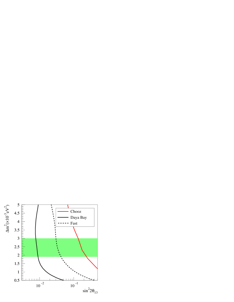
Figure 3.12: Expected $\sin^{2}2\theta_{13}$ sensitivity at 90% C.L. with 3 years of data, as shown in solid black line. The dashed line shows the sensitivity of a fast measurement with the DYB near site and mid site only. The red line shows the current upper limit measured by Chooz.

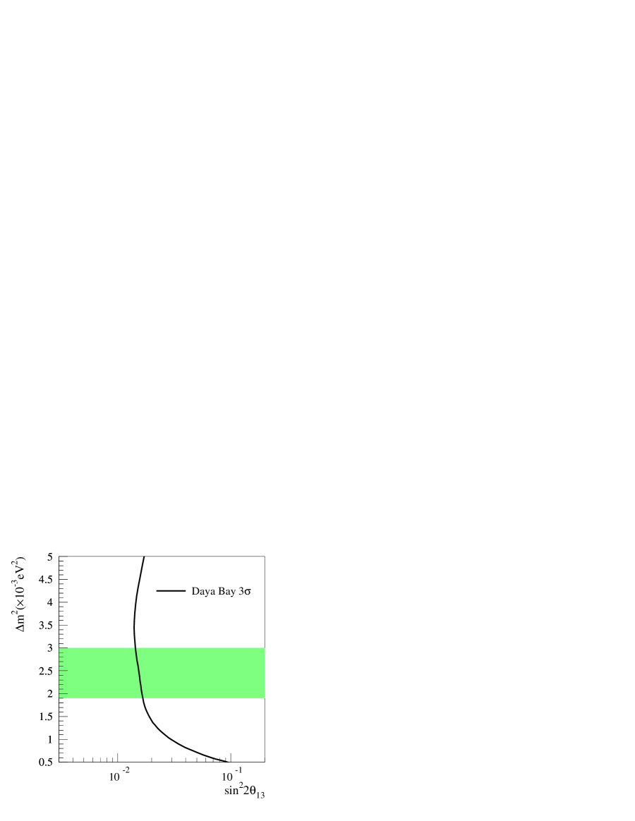
Figure 3.13: Expected 3$\sigma$ discovery limit for $\sin^{2}2\theta_{13}$ at Daya Bay with 3 years of data.

The green shaded area shows the 90% confidence region of $\Delta m^{2}_{31}$ determined by atmospheric neutrino experiments. Assuming four 20-ton modules at the far site and two 20-ton modules at each near site, the statistical uncertainty is around 0.2%. The sensitivity of the Daya Bay experiment with this design can achieve the challenging goal of 0.01 with 90% confidence level over the entire allowed (90% CL) range of $\Delta m^{2}_{31}$. At the best fit $\Delta m^{2}_{31}=2.5\times 10^{-3}$ eV², the sensitivity is around 0.008 with 3 years of data. The corresponding values for other assumptions of systematic uncertainties are shown in Table 3.9.

Systematic Uncertainty Assumptions:	Baseline	Goal	Goal
			with swapping
90% CL Limit:	0.008	0.007	0.006

Table 3.9: 90% CL sensitivity limit for $\sin^{2}2\theta_{13}$ at $\Delta m^{2}_{31}=2.5\times 10^{-3}$ eV² for different assumptions of detector related systematic uncertainties as considered in Section 3.2. We assume 3 years running for each scenario.

Figure 3.13 shows the 3$\sigma$ discovery limit for $\sin^{2}2\theta_{13}$ at Daya Bay with 3 years of data. At $\Delta m^{2}_{31}=2.5\times 10^{-3}$ eV², the corresponding $\sin^{2}2\theta_{13}$ discovery limit is 0.015. Figure 3.14 shows the sensitivity versus time of data taking. After one year of data taking, $\sin^{2}2\theta_{13}$ sensitivity will reach 0.014 (1.4%) at 90% confidence level.

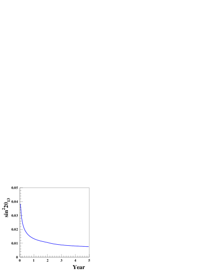
Figure 3.14: Expected $\sin^{2}2\theta_{13}$ sensitivity at 90% C.L. versus year of data taking of the full measurement, with two near sites and one far site. The value of $\Delta m^{2}_{31}$ is taken to be $2.5\times 10^{-3}$ eV².

The tunnel of the Daya Bay experiment will have a total length around 3 km. The tunnelling will take $\sim 2$ years. To accelerate the experiment, the first completed experimental hall, the Daya Bay near hall, can be used for detector commissioning. Furthermore, it is possible to conduct a fast experiment with only two detector sites, the Daya Bay near site and the mid site. For this fast experiment, the ‘far detector’, which is located at the mid hall, is not at the optimal baseline. At the same time, the reactor-related uncertainty would be 0.7%, very large compared with that of the full experiment. However, the sensitivity is still much better than the current best limit of $\sin^{2}2\theta_{13}$. It is noteworthy that the improvement comes from better background shielding and improved experiment design. The sensitivity of the fast option for one year of data taking is shown in the dashed line in Fig. 3.13. With one year of data, the sensitivity is $\sim$0.035 for $\Delta m^{2}=2.5\times 10^{-3}$ eV², compared with the current limit of 0.17 from the Chooz experiment. This fast option will allow us to gain valuable experience and a preliminary physics result while construction is being completed. The higher precision of the completed experiment will be necessary to fully complement the future long baseline accelerator experiments as discussed in Section 1.4.

4 Experimental Site and Laboratories

The Daya Bay site is an ideal place to search for oscillations of antineutrinos from reactors. The nearby mountain range provides excellent overburden to suppress cosmogenic background at the underground experimental halls. Since the Daya Bay nuclear power complex consists of multiple reactor cores, there will be two near detector sites to monitor the yield of antineutrinos from these cores and one far detector site to look for disappearance of antineutrinos. It is possible to instrument another detector site about half way between the near and far detectors to provide independent consistency checks.

The proposed experimental site is located at the east side of the Dapeng peninsula, on the west coast of Daya Bay, where the coastline goes from southwest to northeast (see Fig. 1.13). It is in the Dapeng township of the Longgang Administrative District, Shenzhen Municipality, Guangdong Province. Two mega cities, Hong Kong and Shenzhen are nearby. Shenzhen City is 45 km to the west and Hong Kong is 55 km to the southwest. The geographic location is east longitude 114^∘33’00” and north latitude 22^∘36’00”. Daya Bay is semi-tropical and the climate is dominated by the south Asia tropical monsoon. It is warm and rainy with frequent rainstorms during the typhoon season in one half of the year, while relatively dry in the other half. Frost is rare.

The Daya Bay Nuclear Power Plant (NPP) is situated to the southwest and the Ling Ao NPP to the northeast along the coastline. Each NPP has two cores that are separated by 88 m. The distance between the centers of the two NPPs is about 1100 m. The thermal power, $W_{\rm th}$, of each core is 2.9 GW. Hence the total thermal power available is $W_{\rm th}=11.6$ GW. A third NPP, Ling Ao II, is under construction and scheduled to come online by 2010–2011. This new NPP is built roughly along the line extended from Daya Bay to Ling Ao, about 400 m northeast of Ling Ao. The core type is the same as that of the Ling Ao NPP but with slightly higher thermal power. When the Daya Bay—Ling Ao—Ling Ao II NPP are all in operation, the complex can provide a total thermal power of 17.4 GW.

The site is surrounded to the north by a group of hills which slope upward from southwest to northeast. The slopes of the hills vary from 10^∘ to 45^∘. The ridges roll up and down with smooth round hill tops. Within 2 km of the site the elevation of the hills generally vary from 185 m to 400 m. The summit, called Pai Ya Shan, is 707 m PRD. Due to the construction of the Daya Bay and Ling Ao NPPs, the foothills along the coast from the southwest to the northeast have been levelled to a height of 6.6 m to 20 m PRD. Daya Bay experiment laboratories are located inside the mountain north of the Daya Bay and Ling Ao NPPs.

There is no railway within a radius of 15 km of the site. The highway from Daya Bay NPP to Dapeng Township (Wang Mu) is of second-class grade and 12 m wide. Dapeng Town is connected to Shenzhen, Hong Kong, and the provincial capital Guangzhou by highways which are either of first-class grade or expressways.

There are two maritime shipping lines near the site in Daya Bay, one on the east side and the other on the west side. Oil tankers to and from Nanhai Petrochemical use the east side. Huizhou Harbor, which is located in Daya Bay is 13 km to the north. Two general-purpose 10,000-ton docks were constructed in 1989. Their functions include transporting passengers, dry goods, construction materials, and petroleum products. The ships using these two docks take the west line. The minimum distance from the west line to the power plant site is about 6 km. Two restricted docks of 3000-ton and 5000-ton capacity, respectively, have been constructed on the power plant site during the construction of the Daya Bay NPP [1].

4.1 General Laboratory Facilities

The laboratory facilities include access tunnels connected to the entrance portal, a construction tunnel for waste rock transfer, a main tunnel connecting all the four underground detector halls, a LS filling hall, counting rooms, water and electricity supplies, air ventilation, and communication. There is an assembly hall and control room near the entrance portal on surface. The approximate location of the experiment halls and the layout of the tunnels are shown in Fig. 4.1. All experimental halls are located at similar elevations, approximately $-$20 m PRD.

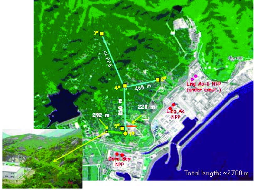
Figure 4.1: Layout of the Daya Bay and Ling Ao cores, the future Ling Ao II cores and possible experiment halls. The entrance portal is shown at the bottom-left. Five experimental halls marked as #1 (Daya Bay near hall), #2 (Ling Ao near hall), #3 (far hall), #4 (mid hall), #5 (LS filling hall) are shown. The green line represents the access tunnel, the blue lines represent the main tunnels and the pink line represents the construction tunnel. The total tunnel length is about 2700 m

.

4.1.1 Tunnels

A sketch of the layout of the tunnels is shown in Fig. 4.2. There are three branches, which are represented by line{3-7-4-5}, line{4-8-Ling Ao near} and line{5-far site}, form the horizontal main tunnel extending from a junction near the mid hall to the near and far underground detector halls. The lines marked as A, B, C, D and E are for the geophysical survey. Line E, which is a dashed line on the top of figure across the far site, is the geophysical survey line investigated if the far site needs to be pushed further from the cores as a result of future optimizations. Line{1-2-3} is the access tunnel with a length of 292 m. Lines B and C are from the survey for the design of the construction tunnel (which may have different options for cost optimization).

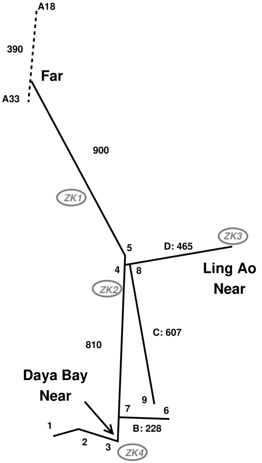
Figure 4.2: Plan view of the experimental halls and tunnels from the site survey (not a detailed tunnel design). All distances are in meters. Line A{1-2-3-7-4-5-far site} has a total length of 2002 m; Line B{7-6} has a total length of 228 m; Line C{8-9} has a total length of 607 m; Line D{4-8-Ling Ao near} has a total length of 465 m. Line E is the dashed line on the top across far site. The four bore hole sites are marked as ZK1, ZK2, ZK3, ZK4 from north to south.

Figure 4.1 shows the entrance portal of the access tunnel behind the on-site hospital and to the west of the Daya Bay near site. From the portal to the Daya Bay near site is a downward slope with a grade of less than 10%. A sloped access tunnel will allow the underground facilities to be located deeper with more overburden.

The access and main tunnels will be able to accommodate vehicles transporting equipment of different size and weight. The grade of the main tunnel will be 0.3% upward from the Daya Bay near hall to the mid hall, and from the mid hall to both the Ling Ao hall and the far hall. The slightly sloped tunnel has two important functions: to ensure a nearly level surface for the movement of the heavy detectors filled with liquid scintillator inside the main tunnel and to channel any water seeping into the tunnel to a collection pit which is located at the lowest point near the Daya Bay near site. The collected water will be pumped to the surface.

The entrance portal of the construction tunnel is near the lower level of the Daya Bay Quarry. The length of this tunnel is 228 m from the entrance to the junction point with the main tunnel if the shortest construction tunnel option is chosen (see Fig. 4.1). During most of the tunnel construction, all the waste rock and dirt is transferred through this tunnel to the outside in order to minimize the interference with the operation of the hospital and speed up the tunnel construction. We expect the access tunnel and the Daya Bay near hall to be finished earlier than the far and Ling Ao halls since it requires much less tunnelling. After the work on this section of tunnel is finished, the Daya Bay near hall will be available for detector installation. Since the construction tunnel is far from the access tunnel and the Daya Bay near hall, we can therefore avoid interference with the rest of the excavation activities and the assembly of detectors in the Daya Bay near site can proceed in parallel. The cross section of the construction tunnel can be smaller than the other tunnels; it is only required to be large enough for rock and dirt transportation. The grade and the length of this construction tunnel will be determined later to optimize the construction cost and schedule.

Excavation will begin from the construction portal. Once it reaches the intersection of the main tunnel, the excavation will proceed in parallel in the directions of the Daya Bay near hall and the mid hall. Once the tunnelling reaches the the mid hall, it will proceed parallel in the direction of the far hall and the Ling Ao hall.

The total length of the tunnel is about 2700 m. The amount of waste to be removed will be about 200,000 m³. About half of the waste will be dumped in the Daya Bay Quarry to provide additional overburden to the Daya near site which is not far away from the Quarry. This requires additional protection slopes and retaining walls. The rest of the waste could be disposed of along with the waste from the construction of the Ling Ao II NPP. Our tunnel waste is about one tenth of the Ling Ao II NPP waste.

4.2 Site Survey

The geological integrity of the Daya Bay site was studied in order to determine its suitability for the construction of the underground experimental halls and the tunnels connecting them. The survey consisted of a set of detailed geological surveys and studies: (1) topographic survey, (2) engineering geological mapping, (3) geophysical exploration, (4) engineering drilling, (5) On-site tests at boreholes and (6) laboratory tests. The site survey has been conducted by the Institute of Geology and Geophysics (IGG) of Chinese Academy of Sciences (CAS). The work started in May 2005 and was completed in June 2006.

4.2.1 Topographic Survey

The topographic survey is essential for determining the position of the tunnels and experimental halls. From the topographic survey the location of the cores relative to the experimental halls is determined, as is the overburden above each of the experimental halls. This measurement of the overburden was input to the optimization of the experimental sensitivity. It is also needed for the portal design and construction. Appropriate maps are constructed out of this measurement. The area surveyed lies to the north of the Daya Bay complex The area of the survey extends 2.5 km in the north-south direction and varies from 450 m to 1.3 km in the east-west direction as determined by the location of the experimental halls and tunnels. The total area measured is 1.839 km². The results of the survey are plotted at a scale of 1:2000.

The instrument used for the topographic measurement is a LEICA TCA2003 Total Station, with a precision of $\pm$0.5” in angle and $\pm$1 mm in distance. Based on four very high standard control points that exist in the area, twenty-six high grade control points and forty-five map baseline points are selected. In total, 7000 points are used to obtain the topographic map. As an example, Fig. 4.3 shows the topographic map around the far site.

Figure 4.3: Topographical map in the vicinity of the far site. The location of the far detector hall is marked by a red square in the middle of the map.

The altitude difference between adjacent contour lines is one meter. The area around the entrance portal, which is behind the local hospital, and the two possible construction portals are measured at the higher resolution of 1:500. The cross sections along the tunnel line for the access and construction portals are measured at an even higher resolution of 1:200. The positions of the experimental halls, the entrance portal, and the construction portal are marked on the topographic map.

4.2.2 Engineering Geological Mapping

Geological mapping has been conducted in an area extending about 2.5 km in the north-south direction and about 3 km in the east-west direction. From an on-the-spot survey to fill in the geological map of the area, a listing of the geological faults, underground water distribution and contact interface between different rocks and weathering zones could be deduced. The statistical information on the orientation of joints is used to deduce the general property of the underground rock, and the determination of the optimal tunnel axes. The survey includes all the areas through which the tunnels will pass and those occupied by the experimental halls. Reconnaissance has been performed along 28 geological routes, of 18.5 km total length. Statistics of 2000 joints and rock mine skeletons are made at 78 spots. Rock mine appraisals are done with 36 sliced samples.

Surface exploration and trenching exposure show that the landforms and terrain are in good condition. There are no karsts, landslides, collapses, mud slides, empty pockets, ground sinking asymmetry, or hot springs that would affect the stability of the site. There are only a few pieces of weathered granite scattered around the region.

The mountain slopes in the experimental area, which vary from $10^{\circ}$ to $30^{\circ}$, are stable and the surface consists mostly of lightly effloresced granite. The rock body is comparatively integrated. Although there is copious rainfall which can cause erosion in this coastal area, there is no evidence of large-scale landslide or collapse in the area under survey. However, there are small-scale isolated collapses due to efflorescence of the granite, rolling and displacement of effloresced spheroid rocks.

The engineering geological survey found mainly four types of rocks in this area: (1) hard nubby and eroded but hard nubby mid-fine grained biotite granite, (2) gray white thick bedding conglomerate and gravel-bearing sandstone, (3) siltstone, (4) sandy conglomerate sandstone. Most of the areas are of hard nubby granite, extended close to the far detector site in the north and reaching to the south, east, and west boundaries of the investigated area. There exists a sub-area, measured about 150 m (north-south) by 100 m (east-west), which contains eroded but still hard nubby granites north of a conspicuous valley existing in this region. Mildly weathered and weathered granites lie on top of the granite layer. Devonian sandstones are located in the north close to the far detector site. There are also scattered sandstones distributed on the top of the granites. The granites are generally very stable, and there exist only three small areas of landslide found around the middle of the above mentioned valley. The total area of the slide is about 20 m² and the thickness is about 1 m. Four faults (F2, F6, F7, F8) and two weathering bags have been identified, as shown in Fig. 4.4

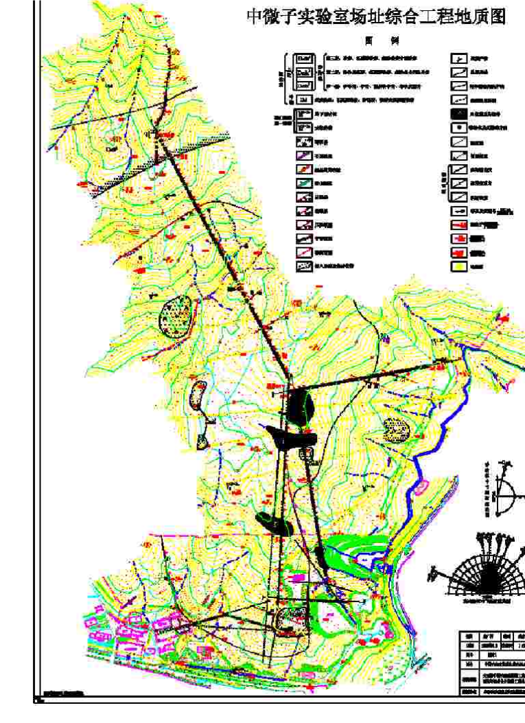
Figure 4.4: Geological map of the experimental site.

The accumulation and distribution of underground water depends generally on the local climate, hydrology, landform, lithology of stratum, and detailed geological structure. In the investigated area of the Daya Bay site, the amount of underground water flux depends, in a complicated way, on the atmospheric precipitation and the underground water seeping that occurs. The sandstone area is rich in underground water seeping in, mainly through joints caused by weathering of crannies that formed in the structure. No circulation is found between the underground water and outside boundary water in this area. Underground water mainly comes from the atmospheric precipitation, and emerges in the low land and is fed into the ocean.

Table 4.1 gives the values of various aspects of the meteorology of the Daya Bay area.

Meteorological Data	Units	Magnitude
Average air speed	m/s	3.29
Yearly dominant wind direction		E
Average temperature	∘C	22.3
Highest temperature	∘C	36.9
Lowest temperature	∘C	3.7
Average relative humidity	%	79
Average pressure	hPa	1012.0
Average rainfall	mm	1990.8

Table 4.1: Average values of meteorological data from the Da Ken station in 1985.

A direct comparison shows that the weather elements in Daya Bay are similar to those in the Hong Kong—Shenzhen area.

According to the historical record up to December 31, 1994, there have been 63 earthquakes above magnitude 4.7 on the Richter scale (RS), including aftershocks, within a radius of 320 km of the site. Among the stronger ones, there was one 7.3 RS, one 7.0 RS, and ten 6.0–6.75 RS. There were 51 medium quakes between 4.7 and 5.9 RS. The strongest, 7.3 RS, took place in Nan Ao, 270 km northeast of Daya Bay, in 1918. The most recent one in 1969 in Yang Jiang at 6.4 RS. In addition, there have been earthquakes in the southeast of China and one 7.3 RS quake occurred in the Taiwan Strait on Sept. 16, 1994. The epicenters of the quakes were at a depth of roughly 5 to 25 km. These statistics show that the seismic activities in this region originate from shallow sources which lie in the earth crust. The strength of the quakes generally decreases from the ocean shelf to inland.

Within a radius of 25 km of the experimental site, there is no record of earth quakes of ${\rm M_{s}}\geq 3.0~{}({\rm M_{L}}\geq 3.5)$, and there is no record of even weak quakes within 5 km of the site. The distribution of the weak quakes is isolated in time and separated in space from one another, and without any obvious pattern of regularity.

According to the Ling Ao NPP site selection report [3], activity in the seismic belt of the southeast sea has shown a decreasing trend. In the next one hundred years, this region will be in a residual energy-releasing period to be followed by a calm period. It is expected that no earthquake greater than 7 RS will likely occur within a radius of 300 km around the site; the strongest seismic activity will be no more than 6 RS. In conclusion, the experimental site is in a good region above the lithosphere, as was argued when the NPP site was selected.

4.2.3 Geophysical Exploration

Three methods are commonly used in geophysical prospecting: high density electrical resistivity method, high resolution gravity method, and seismic refraction image method using a mechanical hammer. The first two methods together with the third as supplement have been used for the Daya Bay geophysical study. The combination of these three methods reveal the underground structure, including: faults, type of granite, rock mine contact interface, weathering zone interface and underground water distribution.

Geophysical exploration revealed another four faults (F1, F3, F4, F5 shown in Fig. 4.4) along the tunnel lines. Figure 4.5 shows the regions of the geophysical survey, including the experimental halls and tunnel sections from the Daya Bay near hall to the mid hall and the far hall. The experimental halls, tunnel sections, faults and weathering bags are marked explicitly in the figure.

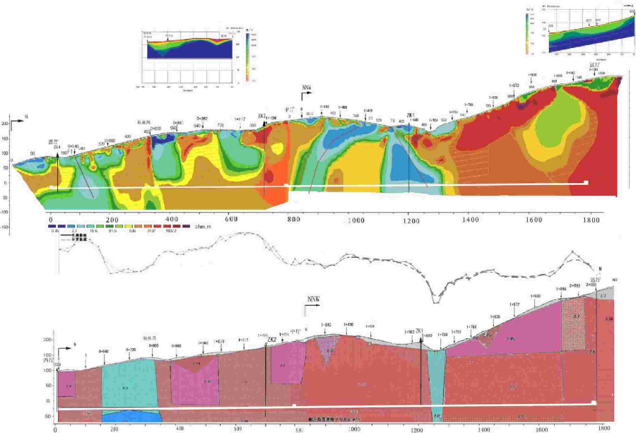
Figure 4.5: Seismic refraction, electrical resistivity and high resolution density maps along the tunnel cross section from the Daya Bay experimental hall (left end) to the far hall (right end).

The electrical resistivity measurements are shown in the middle of the figure, the high resolution density measurements on the bottom, and two sections of seismic refraction measurement in the corresponding part on the top. Because of the complexity and variety of underground structures, the electrical resistivity was measured in boreholes ZK1 and ZK2. The resistivity and density of the rock samples from the boreholes were used for calibration of the resistivity map. Depending on the characteristics of the granite and its geological structure, the electrical resistivity of this area can vary from tens of ohm-m to more than 10k ohm-m. The non-weathered granite has the highest electrical resistivity, whereas the sandstone has medium resistivity due to trapped moisture. The weathered zone, consisting of weathered bursa and faults, has relatively low resistivity.

4.2.4 Engineering Drilling

Based on the information about faults, zones with relative high density of joints, weathering bags, low resistivity areas revealed from previous geological survey, four borehole positions were determined. The purpose of the boreholes was essentially to prove or exclude the inferences from the previous survey approaches above ground. These four boreholes are labelled as ZK1, ZK2, ZK3, ZK4 from north to south in Fig. 4.2. The depth of the four boreholes are 213.1 m, 210.6 m, 130.3 m, 133.0 m respectively (all to at least the tunnel depth). Figure 4.6 shows sections of rock samples obtained from borehole ZK1.

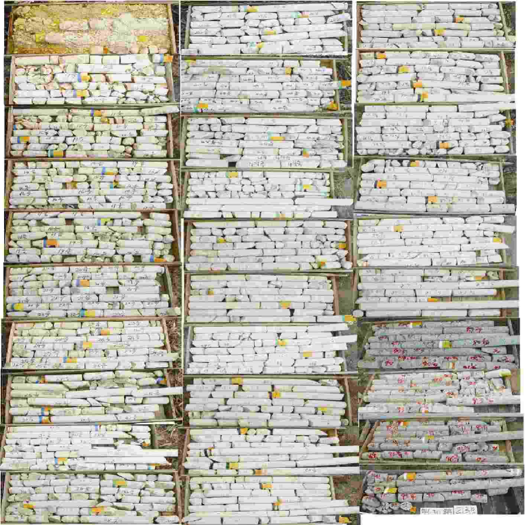
Figure 4.6: Rock samples from borehole ZK1.

Similar samples are obtained in the other three boreholes. The samples are used for various laboratory tests.

4.2.5 On-site Test at Boreholes

There are many on-site tests performed at the boreholes: (1) High density electrical resistivity measurement in boreholes ZK1 and ZK2. (2) Permeability tests at different time and depth are made in the boreholes during borehole drilling and at completion. The test shows that all measured values of the permeability parameter K are less than $0.0009~{}{\rm m/d}$. The K values in ZK2, ZK3 are smaller than that in ZK1 and ZK4. Figure 4.7 shows the water level variation vs time from pouring tests in the four boreholes.

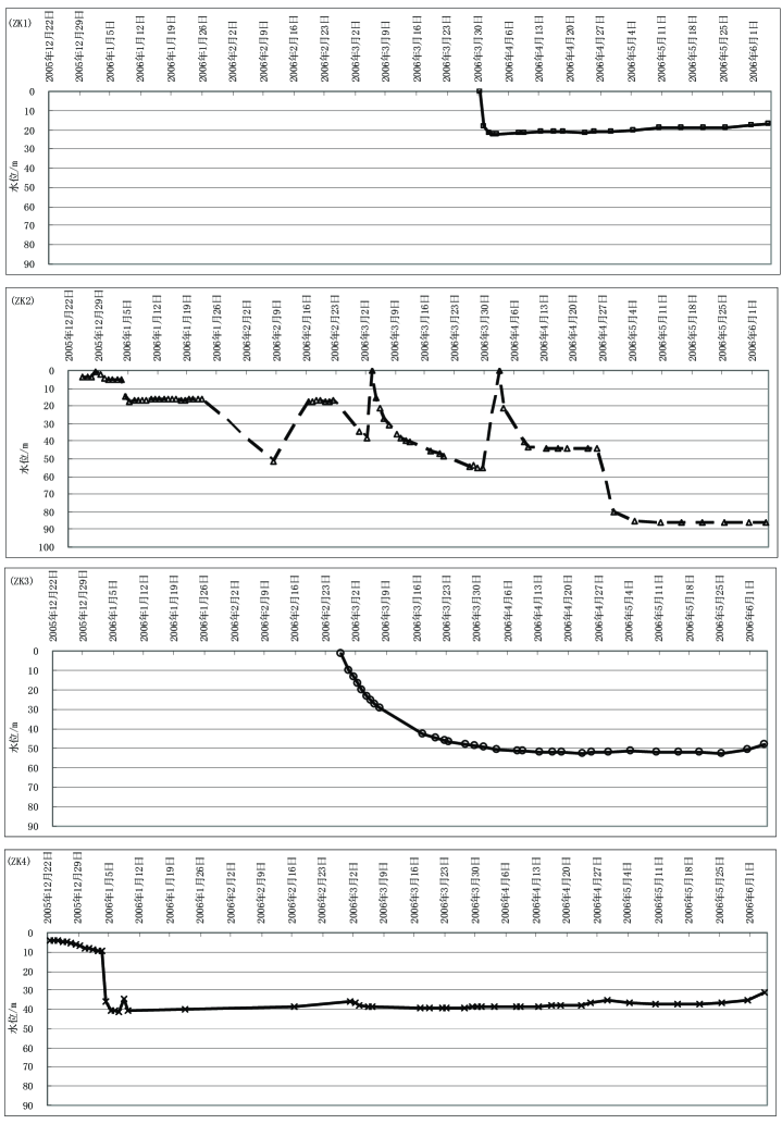
Figure 4.7: Water level variation vs time in the four boreholes. There is no measurement during holidays in January 2006 in ZK2. The cause of the sudden drop of the water level in April 2006 is unknown. The unit of the $x$ coordinate is 7 days, the date reads as year/month/day. The unit of the $y$ coordinate is the water level in meters down the borehole.

(3) Acoustic logging, which is tested at different segments separated by 0.5 m. There are 66, 26, 34, 23 segments tested in ZK1, ZK2, ZK3, ZK4 respectively. The combined results give the velocity of longitudinal wavelength $V_{\rm p}=5500~{}{\rm m/s}$ in the fresh granite. (4) Geo-stress test. (5) Digital video. (6) The radon emanation rate inside the borehole ZK4 was measured up to a depth of 27 m with an electronic radon dosimeter inserted into the borehole. An average rate of $0.58\times 10^{-3}$ Bq m^-2 s^-1 was determined at depths of 14–27 m after correction for back diffusion. These values generally agree with the rates (0.13–2.56)) $\times 10^{-3}$ Bq m^-2 s^-1 measured directly from the rock samples extracted from the borehole. (7) Measurements of the rock chemical composition. The chemical elements of the rock were measured, among these elements, the amount of radioactive U was measured to be 10.7, 16.6, 14.5 and 14.2 ppm from the samples in each of the four boreholes, respectively. The Th concentrations were measured to be 25.2, 49.6, 29.4 and 41.9 ppm in each of the borehole respectively. (8) Water chemical analysis. Water samples from the four boreholes and a surface stream have a pH slightly smaller than 7.5, considered neutral. The water hardness is smaller than 42 mg/l which is considered to be very soft. The underground water is thus very weakly corrosive to the structure of steel, but is not corrosive to reinforced concrete.

4.2.6 Laboratory Tests

Laboratory tests performed includes: rock chemical properties, mineral elements, physical and mechanical property tests. The following data are some of the physical properties of slightly weathered or fresh rock which are the most comment type of rocks in the tunnel construction:

• Density of milled rock: $2.609\sim 2.620~{}g/cm^{3}$

• Density of bulk rock: $2.59\sim 2.60~{}g/cm^{3}$

• Percentage of interstice: $0.765\%\sim 1.495\%$

• Speed of longitudinal wave $(V_{p}):4800\sim 5500~{}m/s$

• Pressure resistance strength of a saturated single stalk: $85.92\sim 131.48~{}MPa$

• Pressure resistance strength of a dry single stalk: $87.88\sim 125.79~{}MPa$

• Softening coefficient: $0.924\sim 1.000$

• Elastic modulus: $32.78\sim 48.97~{}GPa$

• Poisson ratio: $0.163\sim 0.233$

4.2.7 Survey Summary

Based on the combined analyses of the survey and tests described above, IGG concludes that the geological structure of the proposed experimental site is rather simple, consisting mainly of massive, slightly weathered or fresh blocky granite. There are only a few small faults with widths varying from 0.5 m to 2 m, and the affected zone width varies from 10 m to 80 m. There are a total of four weathering bags along the tunnel from the Daya Bay near site to the mid site and on the longer construction tunnel option from the Daya Bay quarry to the mid site. The weathering depth and width are 50–100 m. Just below the surface, the granite is mild to mid weathered. These weathered zones are well above the tunnel, more than three times the tunnel diameter away, so the tunnel is not expected to be affected by these weathering bags. Nevertheless, there are joints around this region and some sections of the tunnel will need extra support.

The far hall at a depth of 350 m is thought to consist of lightly effloresced or fresh granites; the far hall is most likely surrounded by hard granite. The distance to the interface with Devonian sandstone is about 100 m (to the North) from the present analysis estimate.

The rock along the tunnel is lightly effloresced or fresh granite, and mechanical tests found that it is actually hard rock. No circulation is found between the underground water and the outside boundary water in this area, underground water mainly comes from the atmospheric precipitation. Water borehole permeability tests show that underground water circulation is poor and there is no uniform underground water level at the tunnel depth. At the tunnel depth the stress is 10 MPa, which lies in the normal stress regime. The quality of most of the rock mass varies from grade II to grade III (RQD around 70% which indicates good and excellent rock quality). From the ZK1 and ZK2 stress measurements and structure analysis, the orientation of the main compressive stress is NWW. For the east-west oriented excavation tunnel, this is a favorable condition for tunnel stability. For the 810 m segment of the main tunnel from the Daya Bay near hall (#1) to the mid hall (#4) the tunnel orientation will run sub-perpendicular to the orientation of the maximum principal stress and it will thus be subject to higher stress levels at the excavation perimeter. These higher stress levels are not expected to cause significant stability problems due to the strength of the granite rock mass. There are some tunnel sections, including the access tunnel, where the rock mass quality belongs to grade IV, and some belongs to grade V. Figure 4.8 shows the details of the engineering geological section along Line A.

Figure 4.8: Engineering geological section in line A: the faults, weathering bags and tunnel are shown on the figure. The first curve down from the surface shows the boundary of the weathered granite and the second curve down shows the boundary of the slightly weathered granite. The tunnel passes through one region of slightly weathered granite.

Detailed results from the site survey by IGG can be found in references [4, 7, 8, 9, 10, 11, 12].

4.3 Conceptual Design

In June 2006 we organized a bid for a conceptual design of the civil construction. The purpose of this effort was to further refine our understanding of the cost of various options and to make sure that we do not leave any important points out of the final design specifications. The major items of the conceptual design included: (1) the underground experimental halls, the connecting tunnel, access tunnel, and construction tunnel; (2) the infrastructure buildings above ground; (3) the electric power, communication, monitor, ventilation system, water supply, and drainage, safety, blast control, and environmental protection. Two design firms were selected: the Fourth Survey and Design Institute of China Railways (TSY) and the Yellow River Engineering Consulting Co. Ltd. (YREC). TSY has expertise in the design of railway tunnels, and YREC has a great deal of experience in underground hydroelectric engineering projects. They completed their designs in the end of July and beginning of August 2006. These two reports will aide the writing of the specifications of the bid for the detailed tunnel design.

4.3.1 Transportation Vehicle for the Antineutrino Detectors

The biggest item to transport in the tunnel is the antineutrino detector module. Each module is a cylinder of 100 T with an outer diameter 5 m and a height of 5 m, with ports extending above. The transportation of the antineutrino detector determines the cross section of the tunnel and directly affects the total tunnelling construction plan.

The space in the tunnel is limited, so the transportation vehicle for the heavy antineutrino detector should be easy to operate and very stable and smooth during movement. TSY has investigated two kinds of transportation vehicles: (1) heavy-truck with a lowboy trailer, and (2) truck with a platform on top. The bed of the lowboy trailer is 40 cm off the ground and the loading height is 80 cm. The total length of the truck plus the trailer is more than 20 m long, the turnaround radius is 50 m. This turnaround radius makes it impossible to turn the vehicle around without significantly increase the total length of the tunnel. So TSY recommends the use of a truck with a platform on top and the specifications of this platform vehicle available in two manufacturing companies in China are listed in Table 4.2.

Manufacturer	QinHuangDao Heavy	WuHan TianJie special
	Engineering Union Co. Ltd.	transportation Co. Ltd.
Model	TLC100A	TJ100
Full loading(t)	100	100
Out dimension L x W (m)	11.0 x 5.0	11.0 x 5.5
Height of loading (mm)	1700($\pm$300)	1750($\pm$300)
Self weight(t)	28	28
Axles and Wheels/axle	4/8	4/8
Speed	full loading (on flat): 6 km/h	full loading (on flat): 5 km/h
Slope	Vertical 6% Horizontal 4%	Vertical 8% Horizontal 2%
Power	168 kW	235 kW

Table 4.2: Technical parameters of platform trucks.

An example of the platform truck is shown in Fig. 4.9.

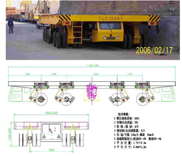
Figure 4.9: Photo of a platform truck with schematic diagrams of wheel rotations. The specifications written in Chinese on the right-bottom are the same as in Table 4.2

It has an easy rotating system with the wheels rotatable in any directions. It has two driving cabs, one in the front and one in the back which makes turning around in the tunnel unnecessary. Its movement is more steady than the lowboy trailer which is very important for transporting the antineutrino detector modules.

YREC also investigated the above mentioned transporting vehicles with similar specifications. In addition, they have investigated an electric railway transportation system which consists of a transport framework, support frame, cable winding, and control desk. However, the loading height is 1 m, and laying the rail is expensive and time consuming. Finally, YREC recommend the use of a semi-trailer with a platform loading, as shown in Fig. 4.10.

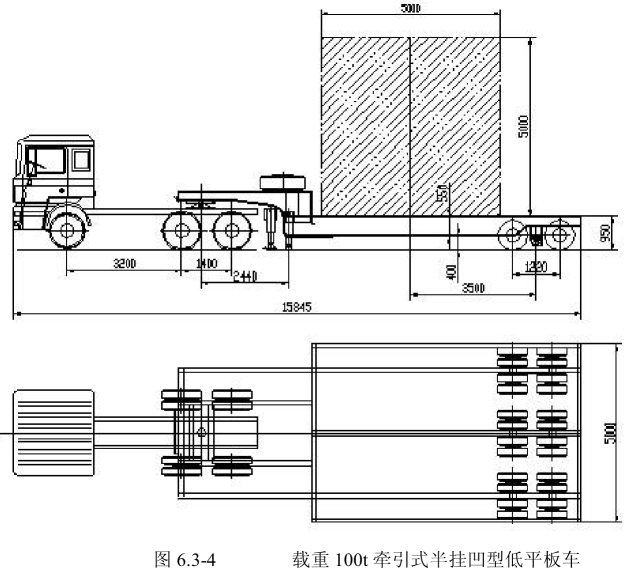
Figure 4.10: Schematic diagram of a semi-trailer. The dimensions, length, width, and height are in mm.

The total length is 15.8 m and the loading height is 95 cm. Since it is not very long, this semi-trailer will drive forward and backward in the tunnel without turning around. The ventilation speed in the tunnel has to be increased during the transportation of the detector modules to vent the exhaust discharged in the tunnel.

Further investigation about the transportation vehicle with lower height of the loading platform is needed in order to lower the required height of the tunnel. It is also necessary to find a suitable electric powered vehicle instead of one powered by petroleum. Current studies are focussing on custom low-boy trailers with electric tugs and on sophisticated, low-profile computer controlled transporters.

4.3.2 Lifting System for the Antineutrino Detectors

Lifting systems, mainly for handling the antineutrino detectors, have been investigated. The lifting system should be low in order to minimize the height of the experimental hall and to gain overburden. Both gantry cranes (suggested by TSY) and bridge style cranes (suggested by YREC) satisfy our requirement. The heights of the experimental halls required to install and lift the antineutrino detector with these two types of cranes are similar: about 12–13 m. Figures 4.11 and 4.12 show these two kind of cranes.

Figure 4.11: Schematic diagrams of a gantry crane in the experimental hall to lift the antineutrino detector (left panel) and lower it into the water pool (right panel).

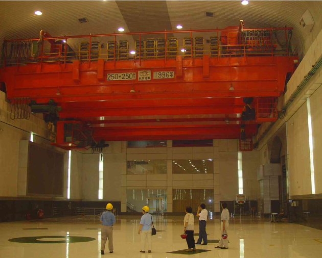
Figure 4.12: A photo of a bridge style crane, the crane rail is fixed to the wall of the experimental hall.

Both cranes have two hooks working during the lifting which will greatly decrease the height of the hall and can be operated more steadily. The final choice of one vs. two hooks needs further study. The rails of the bridge crane are supported on the two side walls of the experiment hall. The final choice of a crane system needs further study.

4.3.3 Experimental Hall Layout

The experimental hall layout can not be fixed before we know how to install the antineutrino detectors, how to lay the muon detectors on top, and what auxiliary facilities are needed. The two designers presented two sketches which include antineutrino detector transportation, lifting space, and rooms for auxiliary facilities, see Fig. 4.13 (designed by TSY)

Figure 4.13: Layout of the experimental hall where the counting room, etc., are laid out in series along the hall (as proposed by TSY).

and Fig. 4.14 (designed by YREC).

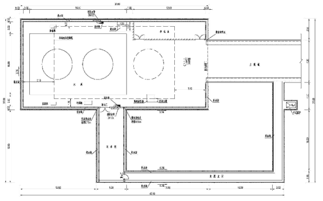
Figure 4.14: Layout of the experimental hall where the counting room, etc., are along one side of the hall (as proposed by YREC).

The auxiliary facilities rooms are at the side of the hall in Fig. 4.14 which may reduce the length of the electronics cables from the detector to the counting room, and other auxiliary facility rooms, which could be arranged parallel to the counting room, are more flexibly arranged. A side tunnel links the main tunnel with the control room and the other possible rooms.

The longitudinal direction of the Daya Bay (#1) and mid (#4) experimental halls is preferred to be along the tunnel direction for construction convenience. The Ling Ao near hall (#2) is the only one with its longitudinal direction to be about 90^∘ with the accessing tunnel in order to keep all the halls in the same orientation.

The LS filling hall (#5) will be decided upon once we settle on the LS mixing and filling procedures. We expect no special questions about the design and construction of this hall. At this stage, we put it near the Daya Bay hall (#1).

4.3.4 Design of Tunnel

According to the size of the selected transportation vehicles, the cross section of the main tunnel will be relatively easy to define:

• Width of the roadway: 5.0 m.

• Width of safety distance to side wall: 1.0 m x 2.

• Width of drainage channel: 0.25 m x 2.

• The total width of the tunnel is: 7.5 m (YREC has 7.0 m because they have a narrower space for safety).

• Height of the transporting vehicle plus height of antineutrino detector: 6.4 m.

• Duct diameter: 1.5 m.

• Safety distance between detector module to the duct: 0.5 m.

• Total height of the tunnel is: 8.4 m (YREC has 8.5 m)

Figures 4.15 and 4.16

Figure 4.15: An engineering schematic diagram of the tunnel layout proposed by TSY. The dimensions are in cm.

Figure 4.16: An engineering schematic diagram of the tunnel layout Proposed by YREC. The dimensions are in meters.

describe the cross sections of the main tunnel. The lining of the tunnel depends on the rock quality. The rock quality varies from grades I to V, grade I being excellent and grade V poor. According to the site survey, more than 90% of the rock belongs to grade I, II or III which are stable rocks. Some very short section of the tunnel have grade IV rock and the only grade V rock is in the first tens of meters at the main portal. The lining for different quality of rocks are giving by two designers in their report [13] [14].

The access tunnel has the same cross section as the main tunnel to enable transportation of the antineutrino detector. This tunnel section has a slope of up to 10%. The antineutrino detector is not yet filled with LS when it is transported down the access tunnel. The length of the tunnel is less than 300 m and modern mining/industrial equipment will have no difficulties in moving on the 9.6% slope of the access tunnel (in the YREC design).

There are two possible design strategies for the construction tunnel. One is to transport the dirt by heavy truck, another one is by tram. In the truck option, the allowed slope is up to 13% (TSY), the width of this tunnel is 5.0 m and height 5.8 m. There will be a passing section in every 80 m along the tunnel for two trucks to cross into the opposite directions. The total length of such a tunnel is 528 m. If a tram is used for dirt transportation, the tunnel can tolerate a much steeper slope, up to 42% ( $<23^{\circ}$ ). The tunnel length can be as short as 200 m and the cross section is 4.6 m wide by 4.08 m high. Construction with a tram will allow for a shorter tunnel, therefore saving both time and money. The dirt removal with a tram is more complicated than using heavy trucks, which will take more time and money. Let us note that in the case of a tram, since special tools are needed, the number of construction companies bidding on the tunnel construction contract may be more limited.

A possible layout of the main portal behind the local hospital is shown in Fig. 4.17 (YREC’s design).

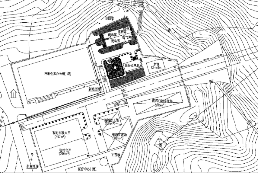
Figure 4.17: A schematic diagram of the the main portal and the layout of auxiliary buildings.

4.3.5 Other Facilities

Other facilities are also included in the conceptual design reports submitted by TSY [13] and YREC [14]. They include: (1) electricity, (2) ventilation system (3) water supply and drainage, (4) communication, (5) monitoring systems, (6) blast control, and (7) environmental effect evaluations.

4.4 Civil Construction Overview

Based in part on the two conceptual design reports, we are optimizing the construction tunnel layout, the crane system, the transport system and the tunnel cross section. Once this process is completed a specification for the final civil construction design package will be drafted. The final tunnel design and civil construction contractors will be selected via a bidding process. Most likely the detailed design and civil construction team will be separated. An oversight agency is needed for the construction. The time needed to complete the final design will be 4–5 months once all of the specifications are laid out. The civil construction will last 1.5–2 years as estimated by the conceptual designers.

The main civil construction work items are listed in Table 4.3.

Construction item	Volume ($m^{3}$)
Excavation dirt in open	17,068
Excavation dirt in tunnel	202,745
Concrete	8,740
Eject concrete	7,774

Table 4.3: Table of the main civil construction work items.

5 Antineutrino Detectors

5.1 Overview

The measurement of $\sin^{2}2\theta_{13}$ to 0.01 or better is an experimental challenge. A value of 0.01 for $\sin^{2}2\theta_{13}$ yields a tiny oscillation effect. This corresponds to a small difference in the number of antineutrino events observed at the far site from the expectation based on the number of events detected at the near site after correcting for the distance under the assumption of no oscillation. To observe such a small change, the detector must be carefully designed following the guidelines discussed in Chapter 2, and possible systematic uncertainties discussed in Chapter 3. The following requirements should be satisfied in the design of the antineutrino detector modules and related components:

1. The detector modules should be homogeneous to minimize edge effects.

2. The energy threshold should be less than 1.0 MeV to be fully efficient for positrons of all energies.

3. The number of protons in the target liquid scintillator should be well known, implying that the scintillator mass and the proton to carbon ratio should be precisely determined. The target scintillator should come from the same batch for each pair of near-far detector modules, and the mixing procedure should be well controlled to ensure that the composition of each antineutrino target is the same.

4. The detector module should not be too large; otherwise, it would be difficult to move from one detector site to another for a cross check to reduce systematic effects. In addition, beyond a certain size, the rate of cosmic-ray muons passing through the detector module is too high to be able to measure the ⁹Li background.

5. The event time should be determined to be better than 25 ns for studying backgrounds.

6. The energy resolution should be better than 15% at 1 MeV. Good energy resolution is desirable for reducing systematic uncertainty (see Chapter 3). It is also important for the study of spectral distortion as a signal of neutrino oscillation.

5.1.1 Module Geometry

Several previous neutrino experiments have designed spherical or ellipsoidal detectors to insure uniform energy response in the entire volume. This type of detector vessel is expensive and requires many PMTs for 4$\pi$ coverage. Two types of alternative detector geometries have been investigated: cubic and cylindrical. Both are attractive from the viewpoint of construction. Monte Carlo simulation shows that a cylindrical shape, as shown in Fig. 2.3, can deliver a better energy and position resolution while maintaining good uniformity of light response over the volume, similar to that of a sphere or ellipsoid. This design is verified by our prototype tests as discussed in section 5.6. An optical reflector can be put at the top and bottom of the cylinder, so that PMTs are only positioned on the circumference of the cylinder, to reduce the number of PMTs by half.

This design, which allows a tremendous reduction of the detector cost including savings on the PMT readout, steel and acrylic vessel construction, is practical due to the following considerations:

1. The event vertex is determined by the center of gravity of the charge, without reliance on time-of-flight, so that the light reflected from the top and bottom of the cylinder will not worsen the performance of the detector module. The individual PMT hit times are measured to a resolution of 0.5 ns for background studies.

2. The fiducial volume is well defined with a three-zone-structure as discussed below wherein no accurate vertex information is needed.

5.1.2 Target Mass

The total target mass at the far site is determined by the sensitivity goal as is shown in Fig. 5.1 as a function of the far site detector mass.

Figure 5.1: Sensitivity of $\sin^{2}2\theta_{13}$ at the 90% C.L. as a function of the target mass at the far site.

To measure $\sin^{2}2\theta_{13}$ to better than 0.01, a total target mass of 80–100 tons is needed, which corresponds to a statistical uncertainty of $\sim$0.2% after three years data taking. A larger target mass is not attractive since the sensitivity improves rather slowly when the target mass goes beyond 100 tons. By adopting a multiple-module-scheme as discussed in Chapter 2, two modules are chosen for each near site to allow a cross check of the module behavior (within the limit of statistic uncertainties at the near site). For the far detector site, at least four modules are needed for sufficient statistics to reach the designed sensitivity while maintaining the number of modules at a manageable level. A detector scheme of eight identical modules, each with a target mass of 20 tons, is chosen. About 600 to 1200 events per day per module will be detected at the Daya Bay near site (300–500 m) with about 90 events per day per module at the far site ($>$1800 m).

5.1.3 Three-zone Antineutrino Detector

A Chooz-type detector with suitable upgrades can in principle fulfill the requirements although completely new concepts are not excluded. The energy threshold of a Chooz-type scintillator detector can be reduced by a three-zone structure as shown in Fig. 5.2.

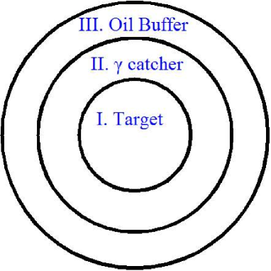
Figure 5.2: Cross section of a simple detector module showing the three-zone antineutrino detector.

The inner-most zone (region I) is the Gd-loaded liquid scintillator antineutrino target. The second zone (region II) is filled with normal liquid scintillator and serves as a $\gamma$-catcher to contain the energy of $\gamma$s from neutron capture or positron annihilation. This zone does not serve as an antineutrino target as neutron-capture on hydrogen does not release sufficient energy to satisfy the 6 MeV neutron detection threshold. The outer-most zone (region III) contains mineral oil that shields radiation from the PMT glass from entering the fiducial volume. This buffer substantially reduces the singles rates and allows the threshold to be lowered below 1.0 MeV. The three regions are partitioned with transparent acrylic tanks so that the target mass contained in region I can be well determined without the need for event vertex reconstruction and a position cut.

5.1.4 $\gamma$-Catcher

The $\gamma$ rays produced in the target region by positron annihilation or neutron capture will undergo many collisions with the LS molecules to transfer most of their energy to the liquid scintillator before converting to visible scintillation light. However, the $\gamma$ rays can also escape from this target region and deposit energy outside of this region. To capture the escaping $\gamma$ rays a layer of undoped liquid scintillator surrounding the target zone is added, significantly reducing this energy loss mechanism. The energy spectrum of the delayed neutron capture signal is shown in Fig. 5.3.

Figure 5.3: The neutron capture energy spectrum in gadolinium as obtained from the GEANT3 simulation. The long tail at low energies corresponds to the escaped events.

The tail to low energies is from events with an escaping $\gamma$. The Gd capture peak at 8 MeV is from the two most abundant isotopes of gadolinium, ¹⁵⁵Gd and ¹⁵⁷Gd, with total $\gamma$ energies of 7.93 and 8.53 MeV, respectively.

A threshold of 6 MeV cleanly separates the 8 MeV neutron capture signal from the background due to natural radioactivity. However, this threshold will cause a loss of some neutron capture events and a corresponding loss of detection efficiency. A simulation of the detector module giving the correlation between the thickness of the $\gamma$-catcher region and the neutron detection efficiency is shown in Fig. 5.4.

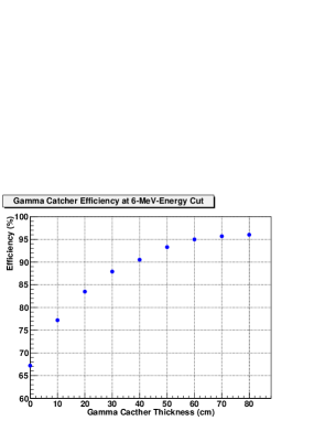
Figure 5.4: The neutron detection efficiency as a function of the $\gamma$-catcher (GCAT). The neutron energy cut is set at 6 MeV. The thickness of the middle zone of the Daya Bay experiment will be 45 cm.

The figure shows that with a $\gamma$-catcher thickness of 45 cm the neutron detection efficiency is 92%. Chooz had a smaller detector and a $\gamma$-catcher thickness of 70 cm, and neutron source test showed a (94.6$\pm$0.4)% detection efficiency [1]. The uncertainty includes a vertex selection uncertainty that Daya Bay will not have. Chooz, Palo Verde and KamLAND all claimed an uncertainty on the energy scale at 6 MeV of better than 1%. Our detector simulation shows that a 1% uncertainty in energy calibration will cause a 0.2% uncertainty in the relative neutron detection efficiencies of different detector modules for a 6 MeV threshold. After subtracting the vertex selection uncertainty, the results of the efficiency test are consistent with simulation. After a comprehensive study of detector size, detection efficiency, and experimental uncertainties, we choose 45 cm as the thickness of the $\gamma$-catcher.

5.1.5 Oil Buffer

The outermost zone of the detector module is composed of mineral oil. The PMTs will be mounted in the mineral oil next to the stainless steel vessel wall, facing radially inward. This mineral oil layer is optically transparent and emits very little scintillation light. There are two primary purposes for this layer: 1) to attenuate radiation from the PMT glass, steel tank and other sources outside of the module; and 2) to ensure that the PMTs are sufficiently far from the liquid scintillator so that the light yield is quite uniform. Simulations indicate that the location of light emission should be at least 15 cm away from the PMT surface, as indicated in Fig. 5.5.

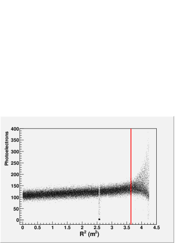
Figure 5.5: Antineutrino detector response (in number of photoelectrons) as a function of radial location of a 1 MeV electron energy deposit. The mineral oil volume has been removed and the PMTs are positioned directly outside the $\gamma$-catcher volume. The vertical red line is 15 cm from the PMT surface and indicates the need for 15 cm of buffer between the PMT surface and the region of active energy deposit in order to maintain uniform detector response.

Simulation shows that with 20 cm of oil buffer between the PMT glass and the liquid scintillator (which corresponds to a 45 cm total oil buffer thickness), the radiation from the PMT glass detected in the liquid scintillator is 7.7 Hz, as summarized in Table 5.1.

		Buffer Oil Thickness
Isotope	Concentration	20 cm	25 cm	30 cm	40 cm
		(Hz)	(Hz)	(Hz)	(Hz)
238U	40 ppb	2.2	1.6	1.1	0.6
232Th	40 ppb	1.0	0.7	0.6	0.3
40K	25 ppb	4.5	3.2	2.2	1.3
Total		7.7	5.5	3.9	2.2

Table 5.1: Radiation from the PMT glass detected in the Gd-scintillator (in Hz) as a function of the oil-buffer thickness (in cm). A 45 cm thick oil buffer will provide 20 cm of shielding against radiation from teh PMT glass.

The welded stainless steel in KamLAND has an average radioactivity of 3 ppb Th, 2 ppb U, 0.2 ppb K, and 15 mBq/kg Co. Assuming the same radioactivity levels for the vessel of the Daya Bay antineutrino detector module, the corresponding rate from a 10-ton welded stainless steel vessel shielding by 45 cm of oil buffer are 3.5 Hz, 2.3 Hz, 0.8 Hz and 2.2 Hz for U/Th/K/Co, respectively at a threshold of 1 MeV. The total is 8.8 Hz. The natural radioactivity of rock, buffer water, mineral oil, dust, radon and krypton in air play a minor role, as described in section 3.4.4. The total $\gamma$ rate is $<$50 Hz.

Since the PMTs are placed in the mineral oil, and the length of PMT plus its base is about 25–30 cm, a 45-cm thick oil buffer will be sufficient to suppress the $\gamma$ rate and the subsequent uncorrelated backgrounds to an acceptable level. The dimensions of the antineutrino detector modules are shown in Table 5.2.

Region	IR(m)	OR(m)	inner height(m)	outer height(m)	thickness(mm)	material
target	0.00	1.60	0.00	3.20	10.0	Gd-LS
$\gamma$-catcher	1.60	2.05	3.20	4.10	15.0	LS
buffer	2.05	2.50	4.10	5.00	8.0–10.0	Mineral oil

Table 5.2: Dimensions of the mechanical structure and materials of the antineutrino detector modules. IR (OR) refers to the inner (outer) radius of each volume and thickness refers to the wall thickness.

The neutrino target is a cylinder of 3.2 m height and 1.6 m radius. The $\gamma$-catcher and oil buffer are both 0.45 m thick. The diameter of the stainless steel vessel is 5.0 m, with a height of 5.0 m and a total mass of 100 tons.

5.1.6 2-zone vs. 3-zone Detector

The possibility of adopting a detector module design with a 2-zone structure, by removing the $\gamma$-catcher from the current 3-zone design, has been carefully studied. A 2-zone detector module with the same outer dimension as the 3-zone structure has a target mass of 40 ton (keeping the same oil buffer and $\gamma$-catcher thicknesses). The efficiency of the neutron energy cut at 6 MeV will be $\sim$70%, compared to $\sim$90% with the $\gamma$-catcher and the 2-zone 40 ton detector module will have only $\sim$60% more detected events than the 3-zone 20 ton detector module. The reduction of efficiency in the neutron energy cut will introduce a larger uncertainty due to the energy scale uncertainty. This uncertainty is irreducible, not removable by the near/far relative measurement, in the different detector modules due to differences in the energy scales.

The energy scale is possibly site-dependent due to variation of calibration conditions in the different sites. According to the experience gained from KamLAND, a 1% energy scale stability at 8 MeV and 2% at 1 MeV can be readily achieved. The uncertainties in neutron detection efficiency for a 1% relative energy scale uncertainty have been studied by Monte Carlo for the 2-zone 40-ton detector module and the 3-zone 20-ton detector module. The uncertainty in the relative neutron detection efficiency for the 2-zone detector module is 0.4% at 6 MeV as compared with 0.22% for the 3-zone detector module. Similar uncertainties at 4 MeV have also been studied, see Table 5.3.

Configuration	6 MeV	4 MeV
2-zone	0.40%	0.26%
3-zone	0.22%	0.07%

Table 5.3: Uncertainty of the neutron energy threshold efficiency caused by uncertainty in the energy scale for 2-zone and 3-zone detector modules. The energy scale uncertainty is taken to be 1% and 1.2% at 6 MeV and 4 MeV, respectively.

This uncertainty will be the dominant residual detector uncertainty (see Table 3.2), while other uncertainties are cancelled by detector module swapping this one is not (e.g., a doubling of this uncertainty will significantly degrade the $\sin^{2}2\theta_{13}$ sensitivity that can be achieved).

As shown in Table 5.3, lowering the energy cut to 4 MeV can reduce the neutron energy threshold efficiency uncertainty. However, the intrinsic radioactivity from the Gd-doped liquid scintillator and the acrylic vessel will cause a significant increase of the accidental background rate. For external sources (such as radioactivity from the PMTs and the rock) only $\gamma$s, with an upper limit of $\sim$3.5 MeV, can enter the detector module. For internal sources, however, $\gamma$s, $\beta$s, and $\alpha$s contribute — these can produce significant rates of signals above 3.5 MeV (e.g. ²⁰⁸Tl has an endpoint of 5 MeV) as observed by KamLAND. Chooz has also observed a significant number of events of delayed energy of 4–6 MeV (see Fig. 5.6).

Figure 5.6: The energy distribution observed by Chooz, horizontal axis is the prompt signal energy; the vertical axis is the delayed signal energy. In the region labelled D there are many background events with delayed signal falling into the 3–5 MeV energy range.

In addition, gadolinium has contamination from ²³²Th which increases the rate of ²⁰⁸Tl decay in the scintillator. All of these factors make a reduction of the neutron threshold from 6 MeV to 4 MeV undesirable. The accidental background rate would be a couple of orders of magnitude larger with the lower threshold at 4 MeV.

5.1.7 Expected Performance

With reflectors at the top and bottom the effective photocathode coverage is 12% with 224 PMTs, the light yield is $\sim$100 p.e./MeV and the energy resolution is around 5.4% at 8 MeV when the total-charge method is used, or 4.5% with a maximum likelihood fit approach. The vertex can also be reconstructed with a resolution similar to a design with 12% PMT coverage on all surfaces. The vertex reconstruction resolution is $\sim$13 cm for a 8 MeV electron event using the maximum likelihood fit, as shown in Fig. 5.7.

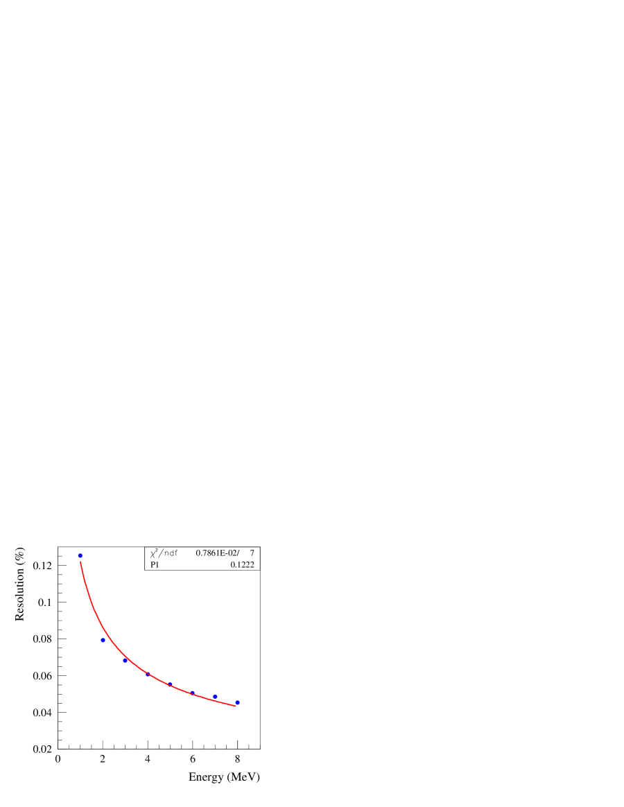
Figure 5.7: Left: The energy reconstruction resolution for electron events uniformly generated in the target region follows $12.2\%/\sqrt{E(MeV)}$. Right: The vertex reconstruction resolution for 8 MeV electron events uniformly generated in the target region using maximum likelihood fitting. The x-axis is the distance of the reconstructed vertex to the true vertex and the y-axis is the number of events.

The horizontal axis is the distance of the reconstructed vertex to the true vertex and the vertical axis is the number of events. Such a vertex resolution is acceptable since the neutron capture vertex has $\sim$20 cm intrinsic smearing, as found by Chooz [1] and by our Monte Carlo simulation as well. The intrinsic smearing of the neutron capture vertex is caused by the energy deposition of the $\gamma$s released from neutron-capture on Gd.

5.2 Containers and Calibration Ports

The stainless steel vessel is the outer tank of the antineutrino detector module, and surrounds the buffer oil region. It will be built with low radioactivity 304L stainless steel and will satisfy the following requirements:

• leak-tight against mineral oil and water over a long period of time (10 years);

• chemically compatible with the mineral oil buffer;

• mechanical strength to support the hydrostatic pressure of the liquids, to support the PMT structure and to handle the stresses induced by transporting, lifting and handling;

• minimal material so as to reduce backgrounds from radioactivity in the steel and welds.

The stainless steel vessel is a cylinder of 5000 mm height and 5000 mm diameter (external dimensions) with a 10 mm wall thickness (304L stainless) as depicted in Fig. 5.8.

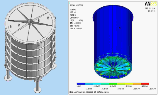
Figure 5.8: 3D view of the stainless steel Buffer vessel.

It weighs about 20 tons (including the support structures) and has a volume of $\sim$95 m³ (without the chimney).

5.2.1 Acrylic Vessel

The target vessel is a cylinder of 3200 mm height and 3200 mm diameter (external dimensions) with 10 mm wall thickness (acrylic). It weighs $\sim$580 kg, and contains a volume of $\sim$25 m³ (without chimneys). The $\gamma$-catcher vessel surrounding the Target is a cylinder of 4100 mm height and 4100 mm diameter (external dimensions) with a 15 mm wall thickness (acrylic). It weighs 1420 kg, and contains a volume of 28 m³ ($53~{}m^{3}-25~{}m^{3}$) (without the chimneys). At the top of the target vessel, there are two or three chimneys for injecting the LS and for passage of radioactive calibration sources. There will be one or two chimneys for the $\gamma$-catcher as well. The chimneys diameter will be $\sim$50–100 mm. Drawings of the target and the $\gamma$-catcher vessels are shown in Fig. 5.9.

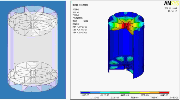
Figure 5.9: The design of the double vessel.

The target and $\gamma$-catcher vessels will be built of acrylic which is transparent to photons with wavelength above $\sim$300 nm (50% at 300 nm [2]). Both vessels are designed to contain aromatic liquids with a long term leak-tightness (free from leakage for ten years) and stability. The critical constraint is the chemical compatibility between the vessel and the scintillating liquids, for at least five years. There must be no degradation of the liquid properties (scintillation efficiency, absorption length) nor any significant degradation of the acrylic material (yellowing or crazing of more than a few percent of the acrylic surface area). The $\gamma$-catcher vessel will also be chemically compatible with the mineral oil in the buffer region.

Acrylic is normally PMMA plus additional ingredients to prevent aging and UV light absorption. Different manufacturing companies have different formulas and trade secrets for the additional ingredients, resulting in different appearance, chemical compatibility, and aging effects. For the material choice, we have surveyed many kinds of organic plastic. We have identified two possible sources for fabrication of the acrylic vessels: the Jiang Chuan Organic Plastic Ltd. Corp, located in city of Lang Fang, Hebei Province, China, and the Gold Aqua System Technical Co. in Kaoshiung, Taiwan (subsidiary of the Nakano company).

The Jiang Chuan Corp. uses a centrifugal casting method for their construction of the vessel. The approach of Nakano’s subsidiary company uses bent plate sheets to be glued together by the polymerization method. It appears at this time that this method will be preferable as it should provide a higher quality vessel.

In the polymerization gluing method, they add the same raw materials as the acrylic (PMMA + ingredients) into the gap between the plates. Thus the joints consist of exactly the same acrylic material as the joined plates, and there is no difference in their mechanical, chemical and optical properties. During polymerization, UV light is used instead of heating, in order to prevent the bent sheets from rebounding. The speed of polymerization is controlled to minimize the remaining stress. Once the tank is fabricated in shape, it will be put in a thermally insulated enclosure for up to a month ($\sim$1 week in our case) to be heated for releasing the stresses. The temperature will be controlled within $\pm 1^{\circ}$ C. Different acrylic types, shapes, thicknesses, etc., need different temperature curves for bending and curing. Hence experience is very important. The geometric precision can be controlled to $\pm$2 mm for a 2 m-diameter tank. The tank can have reinforcement structures at both the top and bottom; therefore the mechanical strength is not a problem for a very thin tank ($\sim$1 cm). However, a thin sheet tends to have more residual stress which may be problematic for chemical compatibility. The minimum thickness of our tank is to be discussed after the compatibility tests of acrylic sheets with liquid scintillator and mineral oil are completed. Figure 5.10 shows a example of the acrylic plastic vessel.

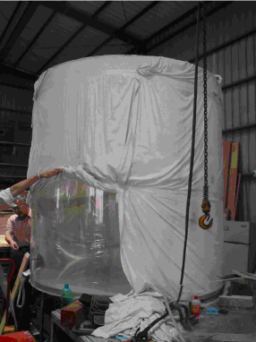
Figure 5.10: A sample acrylic vessel produced at the Gold Aqua Technical Co. in Taiwan. The diameter and the height are both 2 m, with high precision.

Mechanically, the double vessels must be strong and stable enough to ensure identical shapes between near and far target vessels.

The manufacture and transportation of the detector vessels can cause complications to the experiment and they need to be studied in great detail. Simulation has shown that the transportation phase is hazardous for a double acrylic vessel which has been completely assembled. The vessel design, and the design of a transportation system to isolate large shock and vibration loads, requires further analysis. This problem could also be solved, without changing the baseline design, by transporting the target and $\gamma$-catcher vessels separately, and integrate and glue the $\gamma$-catcher top lid and the chimney in the filling hall.

All three regions within the antineutrino detector module have to be filled simultaneously. The filling phase generates constraints related to the differences in height of the liquid. According to mechanical simulations, if we neglect density variations, the acceptable difference in relative fluid heights is 30 cm.

5.2.2 Calibration Ports

In addition to the central chimney port, the buffer vessel lid will have several (3–6) ports, each 100–200 mm diameter, to facilitate the deployment of radioactive calibration sources and light sources. These ports will have gate valves to isolate the calibration devices when they are not in use and facilitate their removal. Around the side wall of the stainless steel vessel there will be 32 ports of 5–10 cm diameter for high voltage, signal, and instrumentation cables.

The cables will be routed down to the bottom of the water pool and up the side so as to minimize interference with the water Cherenkov system. The cables may either be contained in pipes, or we will design a fail-safe isolation connector to allow the cables to be in the water.

5.3 Liquid Scintillator

The gadolinium-loaded organic liquid scintillator, Gd-LS, is a crucial component of the antineutrino detector. The H atoms (”free protons”) in the LS serve as the target for the inverse beta-decay (IBD) reaction, and the Gd atoms produce the delayed coincidence, so important for background reduction, between the prompt positron and the delayed neutron from the IBD. The LS contains $\sim$10% hydrogen. Gd has a very large neutron-capture cross section; the $\sigma$ of natural abundance Gd is 49,000 barns so that isotopic enrichment of the Gd is not required. Two stable isotopes of Gd contribute most of this cross section: $\sigma({{}^{155}}{\rm Gd})=61,400$ barns and $\sigma({{}^{157}}{\rm Gd})=255,000$ barns. Furthermore, neutron-capture on Gd leads to emission of $\gamma$ rays with a total energy of $\sim$8 MeV, that is much higher than the energies of the $\gamma$ rays from natural radioactivity which are normally below 3.5 MeV. Hence, organic LS doped with a small amount of Gd is an ideal antineutrino target and detector. Both Chooz [1] and Palo Verde [3] used 0.1% Gd-doping (1 g Gd per kg LS) that yielded a capture time of $\tau\sim$28 $\mu$s, about a factor of seven shorter than that on protons in undoped liquid scintillator, ($\tau\sim$180 $\mu$s). This shorter capture time reduces the backgrounds from random coincidences by a factor $\sim$7.

To detect reactor antineutrinos with high precision, the Gd-LS must have the following key properties: a) high optical transparency = long optical attenuation length, (b) high photon production (high light yield) by the scintillator, (c) ultra-low impurity content, mainly of the natural radioactive contaminants, such as U, Th, Ra, K, and Rn, and (d) long-term chemical stability, over a period of several years. It is necessary to avoid any chemical decomposition, hydrolysis, formation of colloids, or polymerization, which can lead over time in the LS to development of color, cloudy suspensions, or formation of gels or precipitates, all of which can degrade the optical properties of the LS. To achieve these criteria, R&D is required on a variety of topics, such as: (1) selection of the proper organic LS, (2) development of chemical procedures to synthesize an organo-Gd complex that is soluble and chemically stable in the LS, (3) purification of the components of the Gd-LS, and (4) development of analytical methods to measure these key properties of the Gd-LS over time. These topics will be discussed in the subsections below.

Major R&D efforts on LS and Gd-LS are being carried out at BNL in the U.S., IHEP in the Peoples Republic of China and JINR in Russia:

• The Solar-Neutrino/Nuclear-Chemistry Group in the BNL Chemistry Department has been involved since 2000 in R&D of chemical techniques for synthesizing and characterizing organic liquid scintillators loaded with metallic elements, M-LS. They helped to develop a proposed new low-energy solar-neutrino detector, LENS/Sol [4]. Concentrations of M in the LS $\sim$5-10% by weight were achieved to serve as targets for solar neutrino capture, with M being ytterbium (Yb³⁺) and indium (In³⁺). It was obvious that these chemical results could readily be extended to the new reactor antineutrino experiments, to prepare Gd-LS (with Gd³⁺) at the much lower concentrations required for neutron detection, $\sim$0.1%. BNL began R&D in 2004 on solvent extraction methods to synthesize Gd-LS.

• Nuclear chemists at IHEP also began their R&D on Gd-LS in 2004. They have tended to focus on preparing solid organo-Gd complexes, the idea being that the solid should be readily dissolvable in the LS, to allow preparation of the Gd-LS at the Daya Bay reactor site.

• The JINR chemists, who have long experience in the development of plastic scintillators, are currently studying the characteristics of different LS solvents, especially Linear Alkyl Benzene. They have also began some collaborative work on Gd-LS with chemists at the Institute of Physical Chemistry of the Russian Academy of Sciences, who also did R&D on In-LS for LENS/Sol starting in about 2001.

It should be noted that the general approach of these different groups is pretty much the same, to prepare organo-Gd complexes that are soluble and stable in the LS organic solvent. However, the chemical details of their R&D programs do differ in significant respects at present, such as in the purification procedures, the control of pH, and reliance on either solvent-extraction methods or formation of Gd-precipitates to isolate the Gd organo-complex. We discuss the current status of the major similarities and differences of these approaches. We note that the differences cited do not seriously affect the general goals of the experiment and are acceptable at this stage of development of the experiment. As closer cooperative R&D ties between these groups develop in the coming months, it is expected that these issues will be resolved.

5.3.1 Selection of Solvents

Several aromatic (organic compounds based on benzene) scintillation liquids were studied at BNL to test their applicability as solvents for Gd-LS. (1) Pseudocumene (PC), which is the 1,2,4-isomer of trimethylbenzene (and mesitylene, the 1,3,5-isomer), has been the most commonly used solvent for Gd-LS in previous neutrino experiments. But it has a low flash point (48^∘ C) and aggressively attacks acrylic plastic. (2) Phenylcyclohexane (PCH) has a lower reactivity than PC, but only half of the light yield. (3) Both di-isopropylnaphthalene (DIN) and 1-phenyl-1-xylyl ethane (PXE) have optical absorption bands in the UV region below 450-nm that cannot be removed by our purification procedure (although we note that Double Chooz has chosen PXE as a satisfactory solution for their requirements). (4) Recently, a new LS solvent, Linear Alkyl Benzene (LAB) [5], has been identified as a potentially excellent solvent for Gd-LS. LAB is composed of a linear alkyl chain of 10–13 carbon atoms attached to a benzene ring, and has a light yield comparable to PC. LAB also has a high flash point, which significantly reduces the safety concerns. It is claimed by the manufacturers to be biodegradable, and is relatively inexpensive, since it is used in the industrial manufacturing of detergents. (5) Mineral oil (MO) and dodecane (DD) both have very good light transmission in the UV-visible region so that no further purification is required. They produce little or no scintillating light. It has been reported that mixtures of PC + mineral oil will not attack acrylic.

PC and LAB, as well as mixtures of PC with DD and of LAB with PC, have been selected as the candidate scintillation liquids for loading Gd in the Daya Bay neutrino detector. In China, an unpurified LAB sample obtained from Fushun Petroleum Chemical, Inc. has an attenuation length longer than 30 m; if its quality is uniform from production batch to batch, it can be used directly as the required solvent without further purification. In the U.S., pure LAB has been obtained from the Petresa Company in Canada. Even though this LAB is quite pure, BNL routinely uses purification procedures to ensure that all of its LAB samples have uniform properties. The chemical properties and physical performance of these scintillation solvents, plus mineral oil and dodecane, are summarized in Table 5.4.

LS	Gd Loading	Density	abs430	Purification	Relative	Flash Point
	in LS	(g/cm3)		Method	Light Yield
PC	Yes	0.889	0.002	Distillation	1	48oC
PCH	Yes	0.95	0.001	Column	0.46	99oC
DIN	Yes	0.96	0.023	Column	0.87	$\geq$140oC
PXE	Yes, but is not stable	0.985	0.022	Column	0.87	167oC
LAB	Yes	0.86	0.000	Column	0.98	130oC
MO	No	0.85	0.001	Not needed	NA	215oC
DD	No	0.75	0.000	Not needed	NA	71oC

Table 5.4: Properties of Selected Liquid Scintillators, as compiled at BNL

5.3.2 Preparation of Gadolinium Complexes

One of the major research challenges is how to dissolve the Gd into the liquid scintillator. Since the LS detector is made of an aromatic organic solvent, it is difficult to add inorganic salts of Gd into the organic LS. The only solution to this problem is to form organometallic complexes of Gd with organic ligands that are soluble in the organic LS.

The recent Chooz and Palo Verde antineutrino experiments used different methods to produce their Gd-doped liquid scintillator. In the Chooz experiment, Gd(NO₃)₃ was directly dissolved in the LS, resulting in a scintillator whose attenuation length decreased at a relatively rapid rate, 0.4% per day. As a result, Chooz had to be shut down prematurely. On the other hand, the Palo Verde experiment used the organic complex, Gd-ethylhexanoate, yielding a scintillator which aged at a much slower rate, 0.03% per day.

In the Periodic Table, Gd belongs to the lanthanide (Ln) or rare-earth series of elements. Lanthanides such as Gd can form stable organometallic complexes with ligands that contain oxygen, nitrogen, and phosphorus, such as carboxylic acids, organophosphorus compounds, and beta-diketones. Several recipes for Ln-LS have been developed based on these organic ligands. For example, Gd-ethylhexanoate (Palo Verde, Univ. Sheffield, Bicron), In-, Yb- and Gd-carboxylates (BNL for LENS and Daya Bay), Gd-triethylphosphate (Univ. Sheffield), Yb-dibutyl-butylphosphonate (LENS), and Gd-acetylacetonate (Double-Chooz).

Complexants that have been studied at BNL are (i) carboxylic acids (R-COOH) that can be neutralized with inorganic bases such as NH₄OH to form carboxylate anions that can then complex the Ln³⁺ ion, and (ii) organic phosphorus-oxygen compounds, ”R-P-O”, such as tributyl phosphate (TBP), or trioctyl phosphine oxide (TOPO), that can form complexes with neutral inorganic species such as LnCl₃ [6]. Initially, work was done with the R-P-O compounds. The extraction of Ln is effective, but the attenuation length is only a few meters and the final Ln-LS was not stable for more than a few months. On the other hand, the carboxylic acids, ”RCOOH”, form organic-metal carboxylate complexes that can be loaded into the LS with more than 95% efficiency using solvent-solvent extraction. Moreover the carboxylic acids are preferable because they are less expensive and easier to dispose of as chemical waste, compared to the phosphorus-containing compounds. In principle, the chemical reactions are (a) neutralization, RCOOH + NH₄OH $\rightarrow$ RCOO^- + NH${}_{4}^{+}$+ H₂O in the aqueous phase, followed by (b) Ln-complex formation, Ln³⁺ + 3RCOO${}^{-}\rightarrow$ Ln(RCOO)₃, which is soluble in the organic LS. These reactions are very sensitive to pH: the neutralization step to form the RCOO^- depends on the acidity of the aqueous solution, and hydrolysis of the Ln³⁺ can compete with formation of the Ln(RCOO)₃ complex.

A range of liquid carboxylic acids with alkyl chains containing from 2 to 8 carbons was studied. It was found that acetic acid (C2) and propionic acid (C3) have very low efficiencies for extraction of Ln into the organic phase. Isobutyl acid (C4) and isovaleric acid (C5) both have strong unpleasant odors and require R-P-O ligands to achieve high extraction efficiencies for Ln. Carboxylic acids containing more than 7 carbons are difficult to handle because of their high viscosity; also as the number of carbon atoms increases in the carboxylate complex, the relative concentration by weight of Ln decreases. The best complexant found to date is the C6 compound, 2-methylvaleric acid, C₅H₁₁COOH or ”HMVA”.

Several instrumental and chemical analytical techniques have been used at BNL as guides for optimization of the synthesis procedures for Gd-LS. Besides the measurements of light yield and optical attenuation length to be described below, are measurements in the LS of the concentrations of: (1) Gd³⁺ by spectrophotometry, (2) the total carboxylic acid, R-COOH, by acid-base titrations, (3) the uncomplexed R-COOH by IR spectroscopy, (4) the different organo-Gd complexes in the organic liquid by IR spectroscopy, (5) the H₂O by Karl-Fischer titration, and (6) the NH${}_{4}^{+}$ and Cl^- by electrochemistry with specific ion-sensitive electrodes. These measurements produced very interesting results that indicated that the chemistry of the Gd-LS is more varied and complicated than what is expected from the simple chemical reactions (a) and (b) listed above. The Gd molecular complex in the LS is not simply Gd(MVA)₃, but contains some OH as well, and the form of this complex changes with changing pH. So, even though the long-term studies consistently show that the Gd-LS is chemically stable for periods $\geq$1 year, there is the lingering concern that hydrolysis reactions might occur over long times in the LS. Careful attention to chemical details, especially pH control, is crucial here, as is long-term monitoring of the Gd-LS.

To date at BNL, many hundreds of Ln-LS samples have been synthesized, including scores of Gd-LS. [7] There are two approaches for preparing batches of the Gd-LS: (i) synthesizing each batch at the desired final Gd concentration, 0.1–0.2%, or (ii) synthesizing more concentrated batches, $\geq$1–2% Gd, and then diluting with the organic LS by a factor $\geq$10 to the desired concentration. The two approaches are not identical, with regard to possible long-term effects such as hydrolysis and polymerization. Approach (ii) is currently favored because it simplifies the logistics of preparing and transporting very large volumes of Gd-LS. At IHEP, thirteen organic ligands including four organophosphorus compounds, five carboxylic acids, and four $\beta$-diketones have been tested. The carboxylic acids seem most suitable; three of them have been used for further study. The Gd carboxylate can be synthesized by the following methods: [a.] Carboxylic acids are neutralized by ammonium hydroxide and reacted with GdCl₃ to form a precipitate. The solid is collected by filtration, washed with distilled water, and dried at room temperature. [b.] Carboxylic acids are dissolved in an organic solvent that is also the LS and mixed with a GdCl₃ water solution. Then the pH of the solution is adjusted with ammonium hydroxide. The Gd-carboxylate is simultaneously formed and extracted into the LS solvent. Method [a], the preparation of the solid Gd complex, is currently being emphasized at IHEP.

After the Gd-complex is synthesized and dissolved in the LS, a primary fluorescent additive and a secondary spectrum shifter (both called ”fluors”) are added. At IHEP, the final concentration of the solutes includes 1 g/L Gd, 5 g/L PPO (primary), and 10 mg/L bis-MSB (secondary). The resulting liquid is then pumped through a 0.22-$\mu$m filter and bubbled with nitrogen for the removal of air. At BNL, the fluors, butyl-PBD (3 g/L) and bis-MSB (15 mg/L), are used. No filtration is applied.

5.3.3 Purification of Individual Components for Gd-LS

Most purification steps developed at BNL are applied before and during the synthesis of the Gd-LS [8]. Chemical separation schemes that would be used after the Gd-LS has been synthesized are usually unsuitable because they would likely remove some of the Gd as well as other inorganic impurities.

The removal of non-radioactive chemical impurities can increase the transmission of the light in the LS and enhance the long-term stability of the Gd-LS, since some impurities can induce slow chemical reactions that gradually reduce the transparency of the Gd-LS. Chemical purification steps have been developed for use prior to or during the chemical synthesis: (1) The purification of chemical ingredients in the aqueous phase, such as ammonium hydroxide and ammonium carboxylate, is done by solvent extraction with toluene mixed with tributyl phosphine oxide (TBPO). (2) LAB, which has low volatility, is purified by absorption on a column of activated Al₂O₃. (3) High-volatility liquids, such as the carboxylic acids and PC, are purified by temperature-dependent vacuum distillation at $\leq$0.04 bar. Vacuum distillation should remove any radioisotopic impurities, including radon. Figure 5.11

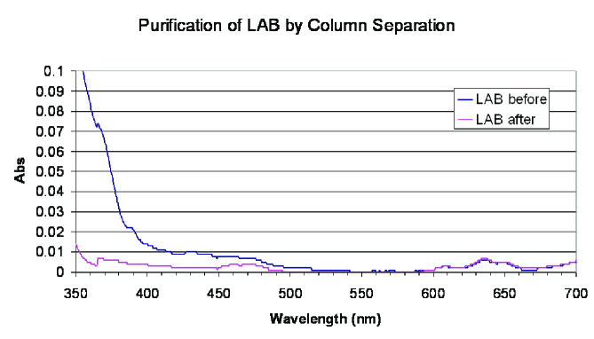
Figure 5.11: UV-visible spectra of LAB before and after purification

compares the optical spectra for LAB before and after purification with the activated Al₂O₃ column.

Two methods, cation exchange and solvent extraction, are being considered at BNL for the purification of radioactive impurities associated with Gd, mainly the U and Th decay chains. The contents of the radioactive impurities in the commercially obtained 99% and 99.999% GdCl₃.6H₂O solids that are used as starting materials were measured by low-level counting at BNL and at the New York State Department of Health and found to be less than the detectable limits (10^-8 g/g). More sophisticated radioactivity measurement steps will have to be developed to quantify these radioactive species at concentrations of 10^-9 g/g in the Gd (implying impurity levels of 10^-12 g/g in the final 0.1% Gd-LS) to fulfill our criterion of a random singles rate below 50 Hz (with 0.8 Hz from radioactive contamination of ²³⁸U, ²³²Th, and ⁴⁰K in the Gd-LS). Although this goal is achievable routinely for unloaded LS (i.e., without added Gd), [9], special care is required for Gd-loaded LS since the Gd (and other lanthanides) obtained in China usually contain ²³²Th at a level of $\sim$0.1 ppm. For Gd loading of 0.1% by weight in the antineutrino detector, the Gd starting material has to be purified to a level $\leq$10^-10g/g. In order to eliminate the Th, Gd₂O₃ powder at IHEP is dissolved in hydrochloric acid and passed through a cation-exchange resin column. Preliminary assays at IHEP showed that this Gd purification procedure reduced the Th content at the ppb level by a factor of four.

5.3.4 Characterization of Gd-LS

The long-term stability of the Gd-LS preparations is periodically monitored in a ”QC”, quality control, program, by measuring their light absorbance and light yield. Samples from the same synthesis batch are sealed respectively in 10-cm optical glass cells for UV absorption measurements, and in scintillation vials for light yield measurements. Monitoring the UV absorption spectrum as a function of time gives a more direct indication of chemical stability than does the light yield. In Fig. 5.12,

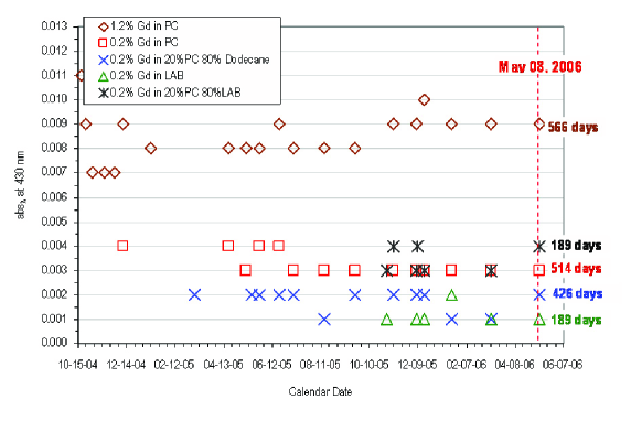
Figure 5.12: The UV absorption values of BNL Gd-LS samples at 430 nm as a function of time

the UV absorption values for a wavelength of 430 nm (in the UV spectrometer) are plotted for BNL Gd-LS samples as a function of calendar date, until May 2006, for different concentrations of Gd from 0.2% to 1.2% by weight in a variety of solvent systems — pure PC, pure LAB, and mixtures of PC+dodecane and of PC+LAB. The figure shows that, since synthesis, samples of: (a) the 1.2% and 0.2% of Gd in pure PC have so far been stable for more than 1.5 and 1 years, respectively; (b) the 0.2% of Gd in the mixture of 20% PC and 80% dodecane has so far been stable for more than a year; and (c) the recently developed 0.2% of Gd in pure LAB and in 20% PC + 80% LAB have been stable so far for approximately 6 months.

The value of the optical attenuation length, $L$, is extrapolated from the UV absorption data. It is defined as the distance at which the light transmitted through the sample has its intensity reduced to $1/e$ of the initial value: $L$ = 0.434 d/a, where $a$ is the absorbance of light (at a reference wavelength, usually 430 nm) measured in an optical cell of length d. Note that for d = 10 cm, a value of $a$ = 0.004 translates into an attenuation length $L$$\sim$11 m. However, it is difficult to extract accurate optical attenuation lengths from these short pathlength measurements because the $a$ values are close to zero. Measurements over much longer pathlengths are needed. BNL has constructed a system with a 1-meter-pathlength, horizontally aligned quartz tube. The light source is a He-Cd, blue laser with $\lambda$ = 442 nm. The light beam is split into two beams with 80% of the light passing through the 1-m tube containing the Gd-LS before arriving at a photodiode detector. The remaining 20% of the light passes through an air-filled 10-cm cell and reaches another photodiode detector to measure the fluctuations of the laser intensity, without any interactions in the liquid. Use of this dual-beam laser system with 1-m pathlength confirmed the values of the attenuation length extrapolated from the measurements with the 10-cm cell in the UV Spectrometer. For 0.2% Gd in a 20% PC + 80% dodecane mixture without fluors, the 1-m measurement gave 99.54% transmission, corresponding to attenuation length $\sim$22 m. This agreed with the value $\sim$21.7 m that was extrapolated from the measured $a$= 0.002 in the 10-cm cell.

The long-term stability of the Gd-LS developed at IHEP has also been investigated with a UV-Vis spectrophotometer using a 10-cm optical cell. IHEP also has developed an optical system with variable vertical pathlengths up to $\sim$2 m to measure the optical attenuation more accurately. Figure 5.13 shows the long term stability over time of four IHEP Gd-LS samples as measured by optical absorption at 430 nm.

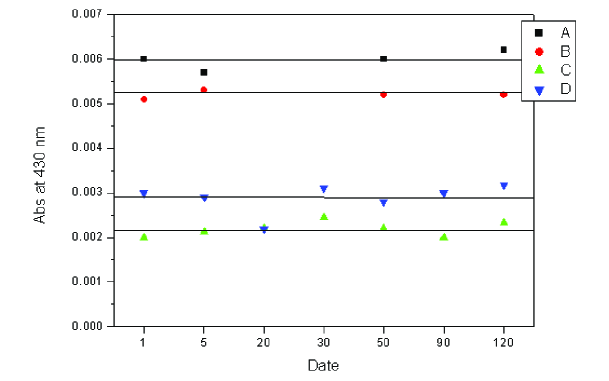
Figure 5.13: Long-term Stability Test: 2 g/L IHEP Gd-LS as a Function of Time.

In all of these IHEP samples, fluors were added, 5 g/L PPO and 10 mg/L bis-MSB. The concentrations of Gd, complexing ligand, and solvent in the four samples are: [A.] 2 g/L Gd, isonanoate as ligand, 4: 6 Mesitylene/dodecane; [B.] 2 g/L Gd, ethylhexanoate as ligand, 2: 8 Mesitylene/dodecane; [C.] 2 g/L Gd, isonanoate as ligand, LAB; [D.] 2 g/L Gd, 2:8 ethylhexanoate as ligand, 2: 8 Mesitylene/LAB; The IHEP results show that the variations of the absorption values are very small during the four-month period for all four samples. The attenuation lengths of samples C and D are longer than 10 m. The IHEP QC program of long-term stability testing will continue for $>$1 year. At JINR, optical properties and light yields of samples of LAB are being measured.

The light yield of the Gd-LS is also measured at BNL and at IHEP. At BNL, a scintillation vial containing ten mL of Gd-LS plus the wavelength-shifting fluors, butyl-PBD (3 g/L) and bis-MSB (15 mg/L), is used for measurement of the photon production. The value of the Gd-LS light yield, which is determined from the Compton-scattering spectrum produced by an external ¹³⁷Cs $\gamma$-ray source that irradiates the sample, is quoted in terms of S%, relative to a value of 100% for pure PC with no Gd loading. Measured S% values are respectively 95% for 95% LAB + 5% PC, and 55% for 0.1% Gd in 20% PC + 80% dodecane.

Table 5.5 lists the light yield for several IHEP Gd-LS samples, relative to a value of 100% for an anthracene crystal.

Gd(g/L)	Scintillator	Complex	Solvent	Light Yield
—	PPO bis-MSB	—	PC:dodecane	0.459
—	PPO bis-MSB	—	LAB	0.542
1.5	PPO bis-MSB	Gd-ethylhexanoate	2:8 PC:LAB	0.538
2.0	PPO bis-MSB	Gd-ethylhexanoate	2:8 PC:LAB	0.528
1.5	PPO bis-MSB	Gd-isononanoic acid	LAB	0.492
2.0	PPO bis-MSB	Gd-isononanoic acid	LAB	0.478

Table 5.5: Light yield for several Gd-LS samples prepared at IHEP, measured relative to an anthracene crystal.

It is seen that the concentration of Gd loading has very little effect on the light yield.

5.3.5 Comparisons with Commercial Gd-LS

At BNL, a sample of commercially available Gd-LS, purchased from Bicron, BC-521, containing 1% Gd in pure PC, has been compared with a BNL Gd-LS sample containing 1.2% Gd in PC. BC-521 is the concentrated Gd-doped scintillator with organic complexing agent in PC that was used in the Palo Verde reactor experiment after it was diluted to 40% PC + 60% mineral oil. The light yields of the respective BNL and Bicron samples were found to be comparable, 82% vs. 85%, when measured at BNL relative to 100% PC, and, as quoted by Bicron, 57% relative to anthracene. However, the attenuation length for the BNL-prepared Gd-LS was $\sim$2.5 times longer than the value for the Bicron BC-521 sample, 6.2 m vs. 2.6 m as measured at BNL; Bicron quoted a value $>$4.0 m for its sample. This significant difference in attenuation may reflect the care put into the BNL pre-synthesis purification steps.

The chemical stability of these BNL and Bicron BC-521 samples are being followed in our QC program. No perceptible worsening of the optical properties of these samples has been observed over periods of 1.5 and $\sim$1 years, respectively. Note that Bicron simply characterizes the stability of its BC-521 as being ”long term”.

5.3.6 Large Scale Production of Gd-LS

Tasks that have begun or will be undertaken in the next several months are as follows: (1) to continue the QC program of long-term stability of different Gd-LS preparations; (2) to determine the quality, quantity, and types of fluors required to add to the Gd-LS to optimize photon production and light attenuation, in order to decide upon a final recipe for the Gd-LS synthesis; (3) to build a closed synthesis system that eliminates exposure of the Gd-LS to air; (4) to scale the chemical procedures for Gd-LS synthesis up from the current lab-bench scale to volumes of several hundred liters, for prototype detector module studies, and as a prelude to industrial-scale production on the level of 160 tons; (5) to automate many of these chemical procedures, which are currently done by hand; (6) to use standardized ASTM-type tests to study the chemical compatibility of the LS with the materials that will be used to construct the detector vessel, e.g., acrylic; (7) to find methods to measure accurately, with high precision, the concentration ratios, C/H and Gd/H, and the H and C concentrations.

5.3.7 Storing and Handling of LS at Daya Bay

The basic assumptions that underlie the following discussion are that we will select LAB as our LS choice. If another scintillator is chosen, the procedures will be modified appropriately. The procedures described below assume that we will dilute a 1% solution of Gd-LS; if another option is chosen these procedures will be appropriately modified. We also assume:

1. Detector modules will be treated as matched pairs, so that they are known to be as identical as can be prepared. Comparison of any differences in the operating characteristics of these identical detectors will provide crucial information about the control of systematic uncertainties. Thus, at a minimum, 40 tons of 0.1% Gd-LS, well mixed and equilibrated, will have to be prepared at one time, to be able to fill two of the antineutrino detector modules at the same time.

2. To reduce the volume of the required space underground and of the costs of excavations, the ‘stock solutions’ of LAB and of 1% Gd in LAB will be stored on the surface.

3. Some procedures, such as stirring or mixing of a liquid in a tank on surface, will be required to ensure uniformity within that liquid. With that capability in hand, it becomes feasible to dissolve the fluors in the LAB that is stored on the surface.

4. Preparation of the 0.1% Gd in LAB will be done underground prior to filling the inner detector modules.

The following points represent the preferred conceptual option for handling large amounts of organic liquids at the Daya Bay site. The first three subsections deal with conditions on the surface, during transport, and underground, while the fourth section deals with general issues that are relevant to all of the subsections.

Surface LS Handling

• LAB (undoped) storage tank (if possible located not too far from tunnel entrance, but this is not an absolute necessity).

  1. Minimum capacity is 140 tons, the total amount of undoped LAB needed to prepare the solution of 0.1% Gd in LAB that will fill all eight antineutrino detector modules.

  2. If desired, this tank can be large enough to store ALL of the LAB required to fill all of the $\gamma$-catcher regions as well as the antineutrino detector modules. Maximum capacity needed is 400 tons.

  3. This tank will not be for passive storage. It will have to contain some mixing apparatus (e.g., mechanical stirrer or gas bubbling) to ensure uniformity of the contained liquid (assuming that more than one shipment of LAB is received from the manufacturer).

  4. This tank on surface will also be used to dissolve and mix the fluors in LAB.

  5. This tank will require a purification column (containing Al₂O₃) in its inlet line, since the LAB will have to undergo final purification prior to addition of the fluors.

• Storage tank for 1% Gd in LAB that has been synthesized elsewhere.

  1. Capacity of 20 tons.

  2. This tank will also need mixing apparatus, to ensure uniformity of the total volume of liquid.

• Mineral Oil will not need a storage tank on surface. If it is delivered in a tanker truck, it can be moved directly underground. If delivered in drums, the mineral oil will be transferred on the surface to an ISO tank for shipment underground.

Transportation of LS Underground

• As discussed in Section 5.3.7 below, transport of batches of liquids from the tanks of LAB and 1% Gd in LAB on the surface to the underground hall will be done in dedicated ISO containers.

• Dilution of the 1% Gd LAB mixture with LAB will be done in the underground filling hall.

Underground LS Filling

• There will be three tanks, each with 40-ton capacity, and each devoted to use with only one of the liquids that will go into the detector module.

• Each of these three tanks will serve as a filling station, by being outfitted with exit ports that will connect to a centralized, instrumented system with plumbing designed to allow the filling of the three zones of each detector module simultaneously: the inner zone with 0.1% Gd in LAB, the intermediate zone with undoped LAB, the outer zone with mineral oil.

• Two of these tanks will be for intermediate passive storage, i.e., one for undoped LAB and one for mineral oil.

• The third tank will serve as a chemical processing tank, to prepare the 0.1% Gd in LAB, by diluting and mixing the 1% Gd-LAB with the undoped LAB. This tank will contain a mixing apparatus.

General Points Regarding LS Handling

• All tanks containing LAB-based liquids, on surface and underground, will need Teflon-like inner liners. The tanks themselves may be stainless steel or other material. We want to avoid rusting as well as contact of the metal with the organic liquids. The choice of materials may depend on the cost.

• To remove air, all of the tanks will have the capability of gas purging, by bubbling inert gas (such as nitrogen) through the organic liquids in the tanks or by establishing a blanket of inert gas to cover the liquid.

• ISO containers, with thermal insulation or possibly active temperature control, will either be leased or purchased. These have capacities of 5000–9000 gallons. They will be carefully cleaned prior to use. Individual ISO containers will be dedicated to use with particular liquids, one for LAB, one for 1% Gd in LAB, and if needed, one for mineral oil. Their main use will be for transport of the liquids from the surface to underground.

• Procedures will have to be developed for clean transfers of the liquids, both on surface and underground, when hooking up to plumbing, etc., to minimize contamination by dust, dirt, and by air-borne radon.

5.4 Antineutrino Detector Photomultiplier Tubes

Optical photons produced by charged particles or $\gamma$ rays in the antineutrino detector are detected with 224 PMTs submerged in the buffer oil inside the steel vessel. The PMTs are arranged in seven horizontal rings, each with 32 PMTs. The rings are staggered in such a way that the PMTs on two adjacent rings are offset by half the PMT spacing in a ring. Simulation studies indicate the adopted number of PMTs and configuration can provide good energy resolution, about 16% at 1 MeV. From the experience of the other experiments, the failure of PMT in the detector is about 1%. We thus have sufficient number of PMTs in each detector module to ensure reliable performance.

We require the PMT to have a spectral response that matches the emission spectrum of the liquid scintillator and good quantum efficiency for detecting single optical photon at a nominal gain of about $10^{7}$. It is desirable to have good charge response, i.e. the peak-to-valley ratio, for identifying the single photo-electron spectrum from the noise distribution. Since the energy of an event is directly related to the number of optical photons collected, the PMTs operating at the nominal gain must have excellent linearity over a reasonable broad dynamic range. In addition, the dark current, pre-pulse and after pulse should be low to minimize the noise contribution to the energy measurement. Furthermore, the natural radioactivity of the materials of the PMT must be kept low so that the $\gamma$-ray background in the detector module is as small as possible. These specifications will be quantified with simulations and by detailed studies of a small number of PMTs purchased from the manufacturers prior to the production order.

Taking the photo-cathode coverage of the detector module, number of PMTs to be used, and cost into account, we plan to use 20-cm-diameter PMTs for the antineutrino detector modules.

5.4.1 PMT Selection Options

There are currently two candidate photomultiplier tubes for use in the antineutrino detector modules, the Hamamatsu R5912 [10] and the Electron Tubes 9354KB [11]. Both are 2$\pi$ PMTs with a 190 mm-wide photocathode and peak wavelength sensitivity near 400 nm. They are similar in design and construction. However, the R5912 has 10 dynodes while the 9354KB has 12. The Hamamatsu R5912 is an improved version over the R1408, which was used by SNO [12]. The R5912 is used by MILAGRO and AMANDA. Both PMTs will be extensively tested.

The manufacturers will be asked to integrate potted bases and oil-resistant high-voltage and signal cables into the construction of the deliverable products. Also we plan to specify the type of the voltage divider optimized by us for Daya Bay operation, which the manufacturer will build from high radiopurity components and seal in the PMT/base assembly. The final decision on the selection of a specific manufacturer will be made after verifying the compliance with the required level of radiopurity, detailed performance comparisons, and price.

5.4.2 PMT Testing

Uniform performance, stable, reliable and lasting operation of the PMT system are essential to the successful execution of the experiment. These requirements demand a comprehensive program of testing and validation conducted prior to installation and commissioning of the PMTs.

We will ask the selected manufacturer to provide certificates of acceptance for the PMTs. The certificates document measured results, compliant to our specifications, that typically include: cathode and anode luminous sensitivity, cathode blue sensitivity, anode dark current and dark counting rate, operating voltage for a gain of 10⁷, charge response and transit time spread.

Testing and validation of the received PMTs will be conducted using a custom test-stand. An LED will be pulsed to simulate scintillation light. The light will be collected within optical fibers and transported to the PMT. This setup allows us to adjust the intensity and position (on the photocathode) of the light reaching the phototube. The purpose of this exercise is to gather a set of physical parameters for each PMT, such as gain vs. high-voltage, operating voltage at the nominal gain, quantum efficiency, dark rate, transition time spread, and linearity. In addition, test of radio-purity will be made. A couple randomly selected tubes from each batch will be radio-assayed non-destructively. If the K, Th, or U content exceeds the specified level of contaminations, additional randomly selected tubes from the same batch will be radio-assayed. If more PMTs exceed the specified contamination level, the whole batch will be rejected. The collected data will be used in simulation and analysis.

5.4.3 PMT Support Structure

The mechanical support of each PMT is a tripod structure which is mounted on a frame attached to the inner wall of the steel vessel. A tripod is stable and convenient for adjusting the orientation of the PMT. Figure 5.14 shows the support structure. This structure is light and will be made of radio-pure materials. The orientation of the PMT can be adjusted by varying the lengths of the three legs. The circular grips provide reliable support of the PMT in all possible positions relative to the direction of the buoyant force.

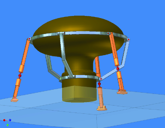
Figure 5.14: PMT mechanical support structure.

5.4.4 High-Voltage System

The high voltage and its control system is designed around an Analog Devices’ variant of the 8052 microcontroller. It functions for both HV control and monitoring. The system is capable of 0.5 V resolution up to 2048 V. An EMCO DC-to-DC HV generator [13] will be mounted near the phototube and will act as our voltage source. The EMCO chips have low ripple, good regulation, and are economical. The base will be a simple tapered divider design mounted directly to the phototube, having a footprint smaller than the standard socket provided by each manufacturer.

Control software is currently written using LabView. The design of this unit is a modified version of the STAR EMC (4800 towers) code, which allowed for 4096 units to be controlled from a single serial port (plus a RS485 converter) in a multi-drop, master-slave network using an RS485 bus. RS485 repeaters will be used to connect various branches of the HV control network to the main control bus. The firmware on the microcontroller and the LabView based control program are both available.

5.5 Front End Electronics

The antineutrino detector readout system is designed to process the PMT output signals. The essential functions are as follows:

• Determine the charge of each PMT signal to measure the energy deposit in the liquid scintillator. This will enable us to select neutrino events, reject backgrounds and deduce the neutrino energy spectrum.

• Determine the event time by measuring arrival time of the signals to the PMTs in order to build the time correlation between prompt and delayed sub-event. The timing information can also help us to reconstruct the location of the antineutrino interaction in the detector, and to study and reject potential background events.

• Provide fast information to the trigger system.

5.5.1 Front-End Electronics Specifications

When a reactor antineutrino interacts in the target, its energy is converted into ultraviolet or visible light, some of which will ultimately be transformed into photoelectrons (p.e.) at the photocathodes of the PMTs. For a given PMT, the minimal number of p.e.’s is one and, based on Monte Carlo simulation, the maximum number is 50 when an antineutrino interaction occurs in the vicinity of the interface between the Gd-doped liquid scintillator and the $\gamma$-catcher. Since typically 500 p.e.’s will be recorded by PMTs for a cosmic-ray muon passing through the detector, the dynamic range of the PMTs is required to be up to about 500 p.e.’s. The intrinsic energy resolution for a single p.e. is typically about 40% with some variation from PMT to PMT, while the energy threshold of a PMT is constrained by the dark noise, typically at the level of about 1/3–1/4 of a p.e. The peak-to-peak noise and the charge resolution of the PMT readout electronics is thus required to be less than 1/10 of a p.e. in both cases. The total charge measurement determined by the center-of-gravity method will produce the total energy deposited by an antineutrino signal or a background event.

The arrival time of the signal from the PMT will be measured relative to a common stop signal, for example, the trigger signal. The time jitter of a PMT for a single p.e. is about 1–2 ns, caused by the PMT transit time jitter, the PMT rise time, and the time walk effect of the signal, etc. The design goal for the time resolution of the readout electronics is thus determined to be less than 0.5 ns.

Since an antineutrino event is a coincidence of the prompt and delayed sub-event, their time interval is a crucial parameter for physics analysis. The precision of this interval is dominated by the trigger signal which is synchronized to the 100 MHz system clock. Hence a 10 ns precision is expected, which is sufficient given the fact that the coincidence window of sub-events is 200 $\mu$s and the resultant uncertainty in efficiency is less than 0.03%. If a TDC counter is employed at the trigger board to measure the actual trigger arrival time with respect to the system clock, a better precision can be achieved.

The dynamic range of the time measurement depends on the uncertainty of the trigger latency and the maximum time difference between the earliest and the latest arrival time of light to PMTs. The range is chosen to be from 0 to 500 ns.

The time measurement of the individual PMT time can also be used to determine the event vertex. Although such a method is particularly suitable for large detectors similar to KamLAND, it provides an independent measurement which complements the charge-gravity method for small detectors with diameters of several meters. Hence it offers a cross-check of systematic uncertainties and an additional handle for studying backgrounds. The readout electronics specifications are summarized in Table 5.6.

Quantity	Specification
Dynamic range	0–500 p.e.
Charge resolution	$<$ 10% @ 1 p.e.
	0.025% @ 400 p.e.
noise	$<$ 10% @ 1 p.e.
Digitization resolution	14 bits
Time range	0–500 ns
Time resolution	$<$ 500 ps
Sampling rate	40 MHz
Channels/module	16
VME standard	VME64xp-340 mm

Table 5.6: Readout Electronics Specifications.

5.5.2 Front End Boards

Each detector module is designed to have a readout system without any relationship to the other modules except receiving a common clock signal and GPS information. The positron and neutron triggers are both recorded with time stamps and the their matching in time will be done offline by software. The readout electronics for each detector module is housed in a 9U VME crate, each can handle up to 16 readout modules, one trigger module, and one or two fan-out modules. In such an arrangement, moveable modules can be easily realized, and correlations among modules can be minimized.

Each readout module receives 16 channels of PMT signals and completes the time and charge measurement. The sum of hit numbers and the total energy of this module is fed into the trigger system for a fast decision. After collecting information from all readout modules, a trigger signal may send to all readout modules for data readout upon a positive decision.

A simplified circuit diagram of the electronic readout system, showing its main functions, is given in Fig. 5.15.

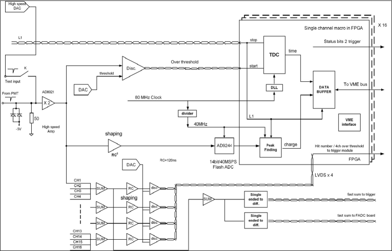
Figure 5.15: Block diagram of front-end electronics module for the antineutrino detector.

The analog signal from a PMT is amplified with a fast, low noise (FET input stage) amplifier. The output of the amplifier is split into two branches, one for time measurement, and the other for charge measurement.

The signal for time measurement is first sent to a fast discriminator with a programmable threshold to generate a timing pulse, whose leading edge defines the arrival time of the signal. A stable threshold set by a 14-bit DAC (AD7247) [14] via the VME controller is needed for the discrimination in order to achieve the required time resolution.

The timing pulse is sent to a TDC as the start signal, while the trigger signal is used as the common stop. The TDC is realized by using internal resources of a high-performance FPGA with key components of two ultra high speed Gray-code counters. The first counter changes at the rising edge of the 320 MHz clock, while the second one changes at the falling edge. Thus, the time bin is 1.5625 ns and the RMS of the time resolution is less than 0.5 ns.

To measure the charge of a PMT signal, an ultra low-noise FET input amplifier (AD8066) is selected for the charge integrator. A passive RC differentiator is used after the integrator to narrow the signal. Since the signal rate of a typical PMT is about 5 kHz including noise, a 300 ns shaping time is chosen, corresponding to an output signal width of less than 1 $\mu$s. The analog signal is accurately digitized by a 14-bit Flash ADC with 40 MHz sampling rate after a baseline recovering. The digitized result goes directly into FPGA, in which all data-processing like data pipelining, pedestal subtraction, nonlinearity correction, and data buffering are implemented.

The readout module has a standard VME A24:D32 interface. Both ADC and TDC data of the triggered event are sent to a buffer, which can store a maximum of 256 events. The data will be readout through the VME backplane by the DAQ system within a reasonable time span.

5.6 Antineutrino Detector Prototype

Valuable data on the performance of the antineutrino detector has been obtained from a scaled down prototype at at the Institute of High Energy Physics, Beijing, China. The goal of this R&D work is multifold: 1) to verify the detector design principles such as reflectors at the top and the bottom, uniformity of the response in a cylinder, energy and position resolution of the detector, etc.; 2) to study the structure of the antineutrino detector; 3) to investigate the long term stability of the liquid scintillator; 4) to practice detector calibration; 5) to provide necessary information for the Monte Carlo simulation.

5.6.1 Prototype Detector Design

As shown in Fig. 5.16, the prototype consists of two cylinders: the inner cylinder is a transparent acrylic vessel 0.9 m in diameter and 1 m in height with 1 cm wall thickness. The outer cylinder is 2 m in diameter and 2 m in height made of stainless steel. Currently, the acrylic vessel is filled with 0.54 tons of normal liquid scintillator, while Gd-loaded liquid scintillator is planned for the near future. The liquid scintillator consists of 30% mesitylene, 70% mineral oil with 5 g/l PPO and 10 mg/l bis-MSB. The space between the inner and outer vessel is filled with 4.8 tons of mineral oil. A total of 45 8” EMI 9350 and D642 PMTs, arranged in three rings and mounted in a circular supporting structure, are immersed in the mineral oil. The attenuation length of the LS is measured to be 10 m and that of the mineral oil is 13 m.

An optical reflector of Al film is placed at the top and bottom of the cylinder to increase the effective coverage area from 10% to 14%. The scintillator light yield is about 10000 photons/MeV, and the expected detector energy response is about 200 p.e./MeV.

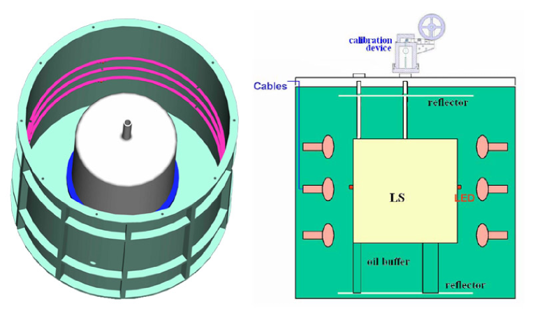
Figure 5.16: Sketch of the antineutrino detector prototype (Left) Top view, (Right) Side view.

The prototype is placed inside a cosmic ray shield with dimensions of 3 m$\times$3 m$\times$3 m. It fully covers five sides (except the bottom). The top is covered by 20 plastic scintillator counters (from the BES Time-of-Flight system), each 15 cm wide $\times$ 3 m long. The four side walls are covered by 36 1.2 m$\times$1.2 m square scintillation counters from the L3C experiment. Figure 5.17 shows a photograph of the prototype test setup, before and after the muon counters were mounted.

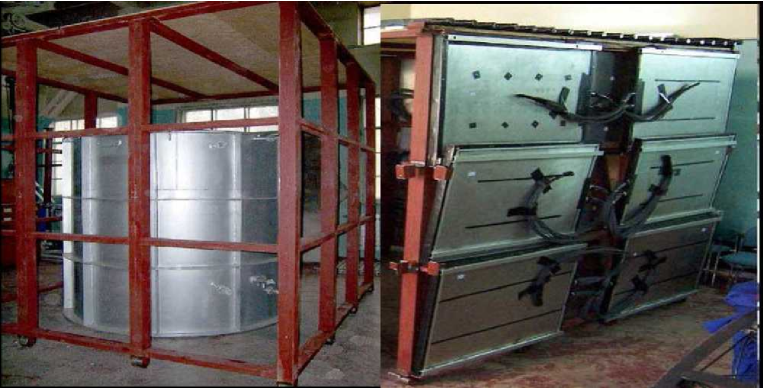
Figure 5.17: The antineutrino detector: before (left) and after (right) the muon detectors were mounted.

The readout electronics were designed as prototypes for the antineutrino detector, according to the requirements discussed in Section 5.5. The trigger system, DAQ system and online software are all assembled as prototypes for the experiment (see Chapter 8).

5.6.2 Prototype Detector Test Results

Several radioactive sources including ¹³³Ba (0.356 MeV), ¹³⁷Cs (0.662 MeV), ⁶⁰Co (1.17+1.33 MeV) and ²²Na (1.022+1.275 MeV) are placed at different locations through a central calibration tube inside the liquid scintillator to study the energy response of the prototype. The gain of all PMTs are calibrated by using LED light sources, and the trigger threshold is set at 30 p.e., corresponding to about 110 keV.

Figure 5.18 shows the energy spectrum after summing up all PMT response for the ¹³⁷Cs and ⁶⁰Co sources located at the center of the detector. A total of about 160 p.e. for ¹³⁷Cs is observed, corresponding to an energy response of 240 p.e./MeV, higher than naive expectations. The energy resolution can be obtained from a fit to the spectra, resulting in a value of about 10%. A detailed Monte Carlo simulation is performed to compare the experimental results with expectations, as shown in Fig. 5.18. Very good agreement is achieved, showing that the detector behavior is well understood.

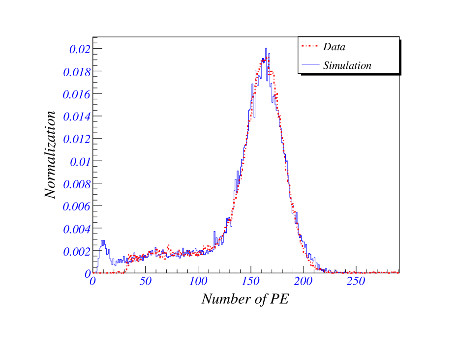
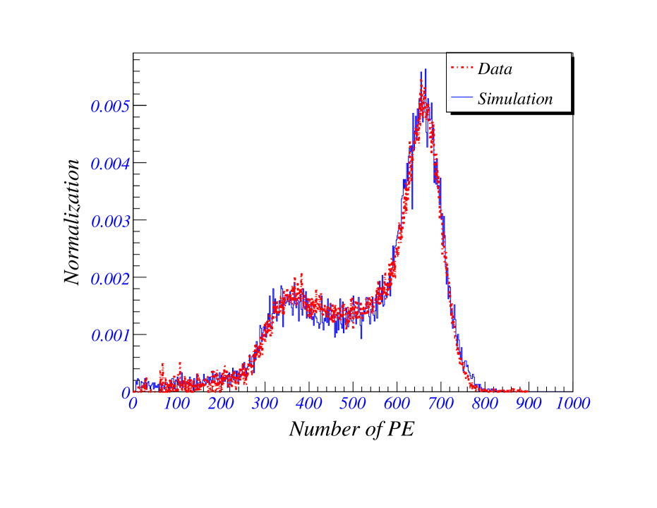
Figure 5.18: Energy response of the prototype to ¹³⁷Cs (left) and ⁶⁰Co (right) sources at the center of the detector with a comparison to Monte Carlo simulation.

All of the sources were inserted into the center of the detector; the energy response is shown in Fig. 5.19 (left). Good linearity is observed, although at low energies non-linear effects are observed which are likely due to light quenching and Cherenkov light emission. The energy resolution at different energies is also shown in Fig. 5.19 (right), following a simple expression of $\sim 9\%/\sqrt{E}$, in good agreement with Monte Carlo simulation as shown in Fig. 5.18.

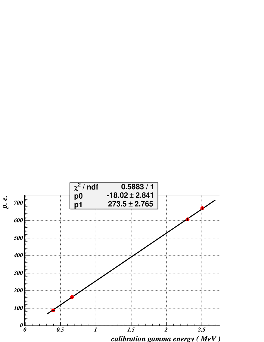
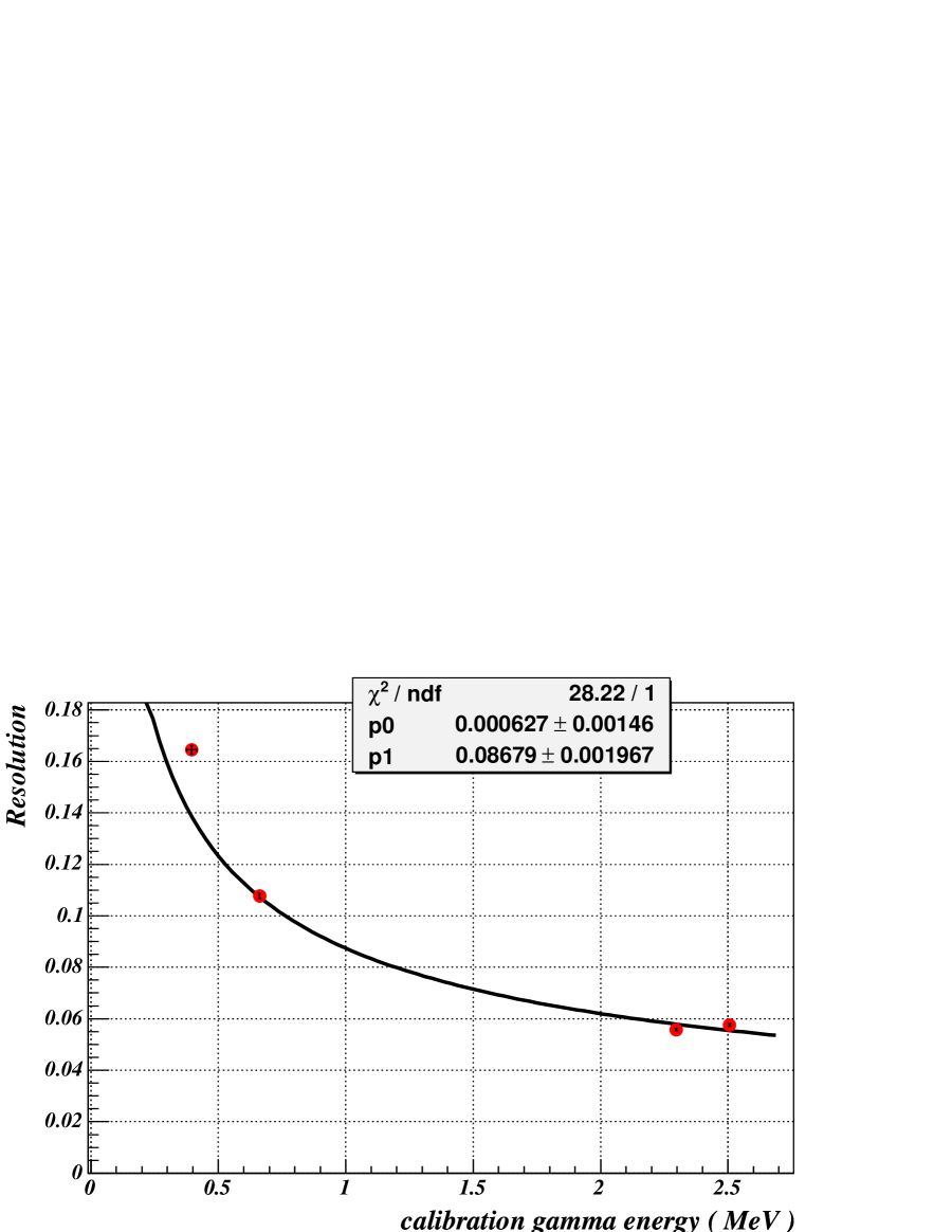
Figure 5.19: Linearity of energy response of the prototype to various sources at the center of the detector (left), and the energy resolution (right).

The energy response as a function of vertical depth along the z-axis is shown in Fig. 5.20. Very good uniformity (better than 10%) over the entire volume of the liquid scintillator shows that the transparency of the liquid is good, and the light reflector at the top and the bottom of the cylinder works well as expected. The fact that the data and Monte Carlo expectation are in good agreement, as shown in Fig. 5.20, demonstrates that the prototype, including its light yield, light transport, liquid scintillator, PMT response, and the readout electronics is largely understood.

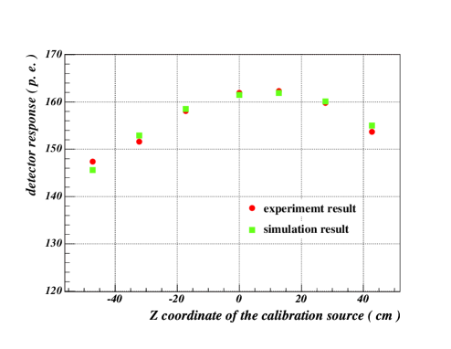
Figure 5.20: Energy response of the prototype to a ¹³⁷Cs source as a function of z position, and a Monte Carlo simulation.

6 Calibration and Monitoring Systems

The measurement of $\sin^{2}2\theta_{13}$ to a precision of 0.01 in the Daya Bay experiment will require extreme care in the characterization of the detector properties as well as frequent monitoring of the detector performance and condition. The physics measurement requires that the neutrino flux be measured with relative precision that is substantially better than 1%. This is accomplished by taking ratios of observed event rates in the detectors at near and far sites to separate the oscillation effect. This will require that differences between detector modules be studied and understood at the level of $\sim$0.1% and that changes in a particular detector module (over time or after relocation at another site) be studied and understood at $\sim$0.1%. Achieving these goals will be accomplished through a comprehensive program of detector calibration and monitoring.

We anticipate a program with three different classes of procedures:

1. “complete” characterization of a detector module,

2. “partial’ characterization, and

3. routine monitoring.

We envision that the complete characterization (procedure #1.) will generally be performed once during initial commissioning of a detector module before taking physics data. Procedure #2 would be employed after relocation of a detector module or after some other change that requires a careful investigation of the detector properties and will involve a subset of the activities in procedure #1. If substantial changes are detected during procedure #2, then we would likely opt for reverting to procedure #1. Finally, procedure #3 will involve both continuous monitoring of some detector parameters as well as frequent (i.e., daily or weekly) automated procedures to acquire data from LED light sources and radioactive sources deployed into the detector volume. The requirements and proposed solutions for procedure #1. are listed in Table 6.1.

Requirement	Description	Proposed Solution(s)
Optical Integrity	Spatial uniformity of response, light attenuation	LED, $\gamma$ sources
PMT gains	Match gains of all PMTs	LED - single p.e. matching
PMT timing	$\sim 1$ ns timing calibration for each PMT	Pulsed LED
Energy scale	Set scale of energy deposition	Gamma sources
H/Gd ratio	Measure relative Gd fraction	252Cf neutron source

Table 6.1: Requirements for the full manual calibration procedure #1.

These will be manually operated procedures using equipment and systems to be described below, and will likely entail several weeks activity.

Procedure #2 will be a subset (to be determined) of the activities in procedure #1 These will be also be manually operated procedures using equipment and systems to be described below, and will likely entail several days activity.

The requirements and proposed solutions for procedure #3 are listed in Table 6.2.

Requirement	Description	Proposed Solution(s)
Mechanical/thermal	Verify these properties are stable	Load sensors, thermometers, etc.
Optical stability	Track variations in light yield	Gamma sources, spallation products
Uniformity, light attenuation	Monitor spatial distribution of light	Gamma sources, spallation products
Detection efficiency	Monitor $\epsilon$ for neutrons and positrons	Gamma sources, neutron sources
PMT gains	Monitor 1 p.e. peaks	LED source

Table 6.2: Requirements for automated calibration procedure #3.

Procedure #3 will entail continuous in-situ monitoring (Sec. 6.3), monitoring of continuously produced spallation-induced activity (Sec. 6.4), and regularly scheduled automated deployment of sources (Sec. 6.5).

6.1 Radioactive Sources

The main goal of the source calibration is to reach the maximum sensitivity to neutrino oscillations by comparing the energy spectra measured by near and far detectors. The response of the detectors at the far and near sites may have small differences, these minute differences can lead to slight distortion in the measured energy spectra of the antineutrinos. Therefore, it is necessary to characterize the detector properties carefully before data taking and monitor the stability of the detectors during the whole experiment. The calibration sources must be deployed regularly throughout the active volume of the detectors to simulate and monitor the detector response to positrons, neutron capture gammas and gammas from the environment.

The sources will be used in the calibration are listed in Table 6.3.

Sources	Calibrations
Neutron sources:	Neutron response, relative and
Am-Be and 252Cf	absolute efficiency, capture time
Positron sources:	Positron response, energy scale
22Na, 68Ge	trigger threshold
Gamma sources:	Energy linearity, stability, resolution
	spatial and temporal variations, quenching effect
137Cs	0.662 MeV
54Mn	0.835 MeV
65Zn	1.351 MeV
40K	1.461 MeV
H neutron capture	2.223 MeV
22Na	annih + 1.275 MeV
60Co	1.173 + 1.333 MeV
208Tl	2.615 MeV
Am-Be	4.43 MeV
238Pu-13C	6.13 MeV
Gd neutron capture	$\sim$ 8 MeV

Table 6.3: Radioactive sources to be used for calibrations.

These sources cover the energy range from about 0.5 MeV to 10 MeV and thus can be used for a thorough energy calibration.

The Am-Be source can be used to calibrate the neutron capture detection efficiency by detecting the 4.43 MeV gamma in coincidence with the neutron. The absolute neutron detection efficiency can be determined with a ²⁵²Cf source, because the neutron multiplicity is known with an accuracy of about 0.3$\%$. In order to absolutely determine the neutron detection efficiency, a small fission chamber will be used to tag neutron events by detecting the fission products. In addition, neutron sources allow us to determine the appropriate thresholds of neutron detection and to measure the neutron capture time for the detectors.

The positron detection can be simulated by a ²²Na source. When a ²²Na source emits a 1.275 MeV gamma, a low energy positron will be emitted along with the gamma and then annihilate. The primary gamma and the following annihilation gammas mimic the antineutrino event inside the detector.

The sources must be encapsulated in a small containers to prevent any possible contamination of the ultra-pure liquid scintillator. They can be regularly deployed to the whole active volume of the detectors and the $\gamma$-catcher.

6.2 LED Calibration System

LEDs have proven to be reliable and stable light sources that can generate fast pulses down to ns widths. They are therefore ideal light sources for checking the optical properties of the liquid scintillator, the performance of the PMTs and the timing characteristics of the data acquisition systems. A schematic diagram of the LED calibration system is shown in Fig. 6.1.

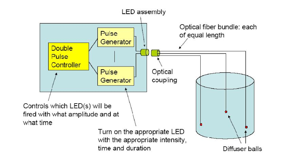
Figure 6.1: Schematic diagram of the LED calibration system.

The LED controller box controls the pulsing of the individual LEDs which are coupled through optical fibers to diffuser balls installed inside the detector module. To ensure consistency among detector modules, a single controller box will be used which can be coupled to the optical fiber bundle of each detector module when needed. Some of the features of the controller box are as follows:

• The pulse heights of each of the double pulses and their separation are fully programmable to simulate the scintillation light produced in an inverse beta-decay interaction. The first pulse will simulate the annihilation photons and direct energy deposition from the positron and the second pulse will simulate the gamma burst resulting from neutron capture on Gd.

• The pulse separation can be generated randomly or stepped gradually.

• The gamma burst can be simulated by simultaneously flashing a number of diffuser balls at various locations inside the detector.

• The controller can be triggered by the muon system to test the detector response following muon events.

The performance of the LEDs will be checked regularly against scintillation produced by a gamma source in a solid scintillator viewed by a PMT. This could be done by coupling the controller box to an optical fiber bundle that is viewed by the same PMT. The number of diffuser balls and their locations inside the central acrylic vessel and the $\gamma$-catcher will be determined through computer simulation. Most of the diffuser balls will be fixed while a few can be moved in the vertical direction by using the same deployment system for radioactive source calibration. The diffuser balls and optical fibers will have to be fully compatible with liquid scintillator.

6.3 In-situ Detector Monitoring

Each detector module will be equipped with a suite of devices to monitor in-situ some of the critical detector properties during all phases of the experiment. The in-situ monitoring includes load and liquid sensors for the detector mass, attenuation length measurements of the Gd-loaded LS target and the LS $\gamma$-catcher, a laser-based monitoring system for the position of the acrylic vessel, accelerometers, temperature sensors, and pressure sensors for the cover gas system. A sampler for routine extraction of a LS sample complements this multi-purpose suite of monitoring tools.

The purpose of these tools is to provide close monitoring of the experiment during three critical phases of the experiment:

1. detector filling

2. data taking

3. detector transport and swapping

During filling of the modules the changing loads and buoyancy forces on the acrylic vessels and the detector support structure are carefully monitored with load and level sensors to ensure that this dynamic process does not exceed any of the specifications for the acrylic vessels.

Most of the time during the duration of the experiment the detectors will be stationary and taking data. Experience from past experiments has shown that the optical properties of detectors will change over time due to changes in the attenuation lengths of the liquid scintillator or changes in the optical properties of the acrylic vessel. It is important to track these characteristics to be able to explain any possibly changes in the overall detector response as determined in the regular, automated calibration. In-situ monitoring of the LS attenuation length and regular extractions of LS samples from the detector modules will help monitor some of the basic detector properties.

The transport of the filled detectors to their location and the swapping of detectors over a distance of up to $\sim$1.5 km is a complex and risky task that will require close monitoring of the structural health of the detectors modules during the move. The proposed swapping scheme of the detectors is a novel method without proof-of-principle yet. While conceptually very powerful, extreme care has to be taken in the calibration and characterization of the detectors before and after the move to be able to correct for all changes in the detector response or efficiencies. The accelerometers, pressure sensors, and the monitoring of the acrylic vessel positions will provide critical real-time information during this procedure to ensure that the detectors – and in particular the acrylic vessels and PMTs – are not put at risk. Recording any changes in the detector modules will also help us understand possible differences in the detector response before and after the move. The acrylic vessel position monitoring system will use a laser beam and reflective target on the acrylic vessel surfaces. By measuring the angular deflection of the laser beam over the length of the detector, transverse displacements of the acrylic vessel can be monitored quite precisely.

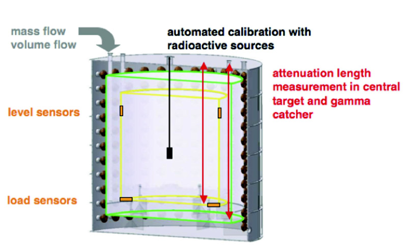
Figure 6.2: Diagram illustrating the variety of monitoring tools to be integrated into the design of the antineutrino detector modules.

6.4 Detector monitoring with data

Cosmic muons passing through the detector modules will produce useful short-lived radioactive isotopes and spallation neutrons. These events will follow the muon signal (detected in the muon system as well as the detector) and will be uniformly distributed throughout the detector volume. Therefore, these provide very useful information on the full detector volume which is complementary to the information obtained by deploying point sources (Sec. 6.5 and 6.6). For example, such events are used by KamLAND to study the energy and position reconstruction as well as to determine the fiducial volume. As with KamLAND, the Daya Bay experiment will use primarily spallation neutron capture and ¹²B decay ($\tau=29.1$ ms and $Q=13.4$ MeV). The rates of these events for Daya Bay are given in Table 6.4.

Event type	Near Site Rate	Far Site Rate
Neutrons	9000/day	400/day
12B	300/day	28/day

Table 6.4: Estimated production rates (per 20 T detector module) for spallation neutron and ¹²B events in the Daya Bay experiment.

Regular monitoring of the full-volume response for these events, compared with the regular automated source deployments, will provide precise information on the stability (particularly of optical properties of the detector, but also general spatial uniformity of response) of the detector modules. With the addition of Monte Carlo simulations, this comparison can be used to accurately assess the relative efficiency of different detector modules as well as the stability of the efficiency of each module.

6.5 Automated Deployment System

Automated deployment systems will be used to monitor all detector modules on a routine (perhaps daily) basis. Each detector module will be instrumented with three (or possibly four) identical automated deployment systems. Each system will be located above a single port on the top of the detector module, and will be capable of deploying four different sources into the detector volume (see Fig. 6.3).

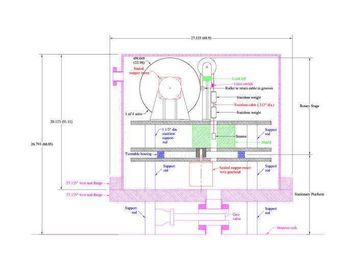
Figure 6.3: Schematic diagram of the automated deployment system concept.

This will be facilitated by four independent stepping-motor driven source deployment units all mounted on a common turntable. The turntable and deployment units will all be enclosed in a sealed stainless steel vessel to maintain the isolated detector module environment from the outside. All internal components must be certified to be compatible with liquid scintillator. The deployment systems will be operated under computer-automated control in coordination with the data acquisition system (to facilitate separation of source monitoring data from physics data). Each source can be withdrawn into a shielded enclosure on the turntable for storage. The deployed source position will be known to about 2 mm.

At present, we anticipate including three radioactive sources on each deployment system:

• ⁶⁸Ge source providing two coincident 0.511 MeV $\gamma$’s to simulate the threshold positron signal,

• ⁶⁰Co source providing a $\gamma$ signal at 2.506 MeV

• ²⁵²Cf fission source to provide neutrons that simulate the neutron capture signal.

These sources can be deployed in sequence by each of the systems on each detector module. During automated calibration/monitoring periods, only one source would be deployed in each detector module at a time. Simulation studies are in progress to determine the minimal number of locations necessary to sufficiently characterize the detector (in combination with spallation product data as discussed in section 6.4). At present we anticipate that three or four radial locations will be sufficient with at least three as follows:

• Central axis

• A radial location in the central Gd-loaded volume near (just inside) the inner cylindrical acrylic vessel wall

• A radial location in the $\gamma$-catcher region.

An additional radial location may be instrumented if it is demonstrated to be necessary by the ongoing simulation studies.

Simulation studies indicate that we can use these regular automated source deployments to track and compensate for changes in:

• average gain of the detector (photoelectron yield per MeV)

• number of PMTs operational

• scintillation light attenuation length

as well as other optical properties of the detector system.

As an example of how the system can be utilized to monitor the attenuation length of the scintillator, Figure 6.4 shows simulations of neutron captures and ⁶⁰Co source deployments.

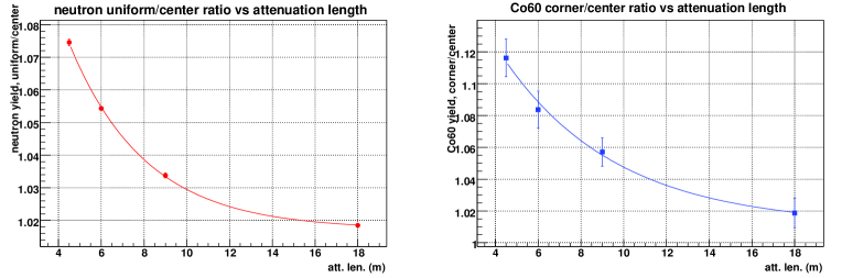
Figure 6.4: The left panel shows how the scintillator attenuation length can be determined from the ratio of the neutron capture peak from spallation neutrons (uniform distribution) to that from a source at the center of the detector. The right panel shows a similar measurement using the ratio of the ⁶⁰Co peak for a source at the center to one at the corner ($r=1.4$ m, $z=1.4$ m) of the central volume (1000 events each).

Both methods can clearly be used to measure the attenuation length of the Gd-loaded liquid scintillator. Thus these methods will provide frequent monitoring of the condition of the scintillator, and will allow us to track changes and differences between detector modules.

6.6 Manual deployment system

A mechanical system will be designed to deploy sources throughout the active volume of the detectors. The source inside the detector can be well controlled and the position can be repeated at a level less than 5 cm. The whole deployment system must be treated carefully to prevent any contamination to the liquid scintillator. The system must be easy to setup and operate, tolerate frequent use and must have a reliable method to put sources into the detectors and to take the sources out as well. The space for operation should not be too large. Figure 6.5 shows a schematic view of the manual source deployment system.

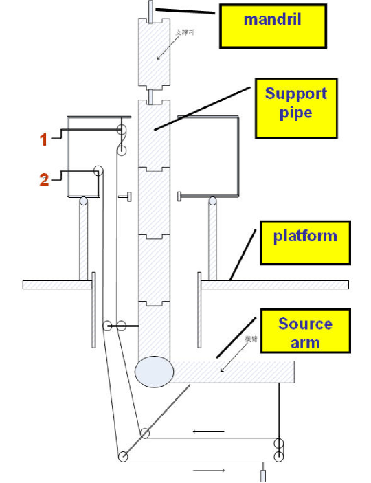
Figure 6.5: Schematic diagram of the manual source deployment system.

The philosophy of such a system is taken from the oil drilling system. The support pipe is separated into several segments. They can be connected one by one to make a long support pipe. This design would reduce the requirement for large space for operations.

The operation procedure will be the following: first, the support pipe and the source arm will be installed in line (vertical). Then, it will be put into the desired position inside the detector, by adjusting the number of segments. When it reach the measurement position, the source arm is turned to the horizontal. After this, the source position can be adjusted by the rope system. The rope system must be designed to insert and remove the sources easily and the position of the source must be accurately controlled. The whole system can be rotated around the axis of the pipe on the platform, thus it can deploy the sources to any position inside the detector.

7 Muon System

The main backgrounds to the Daya Bay Experiment are induced by cosmic-ray muons. These backgrounds are minimized by locating the detectors underground with maximum possible overburden. Background due to muon spallation products at the depths of the experimental halls as well as ambient gamma background due to the radioactivity of the rock surrounding the experimental halls is minimized by shielding the antineutrino detectors with 2.5 meters of water. Gammas in the range of 1–2 MeV are attenuated by a factor $\sim$10 in 50 cm of water [1]. Thus the 2.5 meters of water provides a reduction in the rock gamma flux of approximately five orders of magnitude. This “water buffer” also attenuates the flux of neutrons produced outside the water pool.

Events associated with fast neutrons produced in the water itself remain a major potential background. A system of tracking detectors will be deployed to tag muons that traverse the water buffer. Events with a muon that passes through the water less than 200$\mu$s before the prompt signal, which have a small but finite probability of creating a fake signal event, can be removed from the data sample without incurring excessive deadtime. By measuring the energy spectrum of tagged background events and having precise knowledge of the tagging efficiency of the tracking system, the background from untagged events (due to tagging inefficiency) can be estimated and subtracted statistically with small uncertainty. Our goal is to keep the uncertainty of this background below 0.1%.

The tracking system will also tag events that have a high likelihood to produce other cosmogenic backgrounds, ⁹Li being the most important one. While tagging muon showering events may help to suppress the ⁹Li background, the working assumption is that no extra requirements are imposed on the tracker in order to reduce the ⁹Li background.

The current baseline configuration for meeting these challenges is shown schematically in Fig. 7.1.

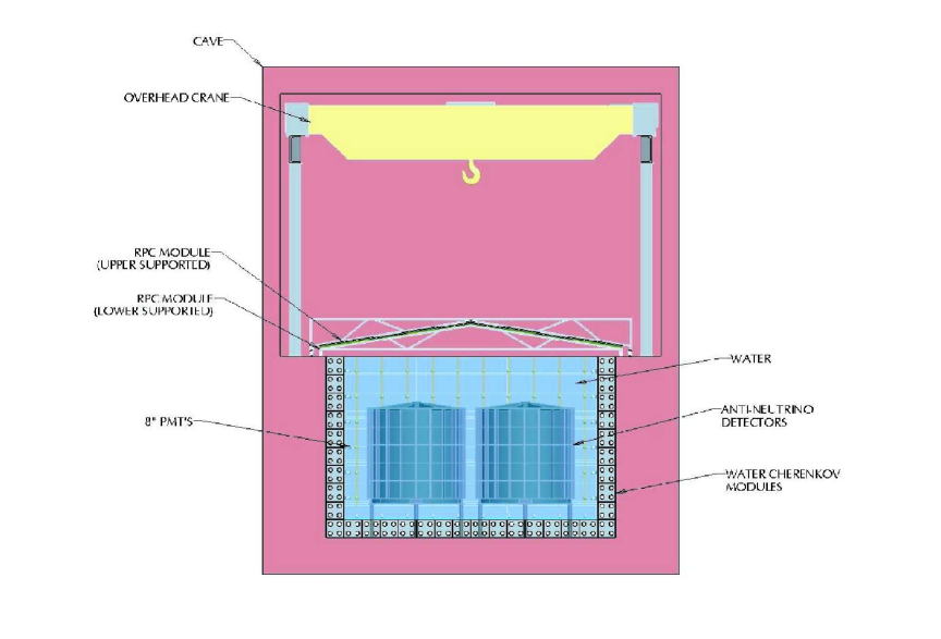
Figure 7.1: Elevation view of an experimental hall.

The antineutrino detectors are separated by 1 m from each other and immersed in a large pool of highly-purified water. The pool is rectangular in the case of the near halls and square in the case of the far hall. The minimum distance between the detectors and the walls of the pool is 2.5 m. The water shield constitutes the inner section of the pool and is instrumented with phototubes to detect Cherenkov photons from muons impinging on the water. The sides and bottom of the pool are lined with 1 m $\times$ 1 m cross-section Water Cherenkov Modules (WCMs) read out by phototubes at either end. The muon tracker is completed by layers of Resistive Plate Chambers (RPCs) above the pool. The top layers extend 1 m beyond the edge of the pool in all directions, both to minimize the gaps in coverage and to allow studies of background caused by muon interactions in the rocks surrounding the pool.

Expected rates of cosmic ray muons in the components of the muon system can be found in Table 8.1.

7.1 Muon System Specifications

Note that it is not envisioned that this system will act as an online veto. This will allow ample opportunity for careful offline studies to optimize the performance of the system.

Requirements of the muon system are summarized in more detail in the following subsections.

7.1.1 Muon Detection Efficiency

The combined efficiency of the muon tracker and the water shield has to exceed 99.5%, with an uncertainty $<$0.25%. This is driven by the need to reject the fast neutron background from muon interactions in the water and to measure its residual level. As can be seen in Table 3.5, without suppression, this background would otherwise be $>$30 times that of the fast neutron background from muon interactions in the surrounding rock, i.e. at a level roughly 2% of that of the signal. A factor 200 reduction in this rate brings the fast neutron background from the water safely below that from the rock, and the total residual fast neutron background down to the 0.1% level. The requirement on the uncertainty in the efficiency brings the systematic due to the uncertainty on the fast neutron background from the water to a level where it is small compared with other systematics.

7.1.2 Muon System Redundancy

It is difficult to achieve the requisite efficiency with only one tracking system. Moreover it is necessary to have a method of measuring the residual level of background after the imposition of the muon rejection cuts. Therefore it is desirable to have two complementary tracking systems to cross check the efficiency of each system.

As discussed below, the current baseline design is to instrument the water shield as a Cherenkov tracker by deploying 8” PMTs in the water with 1.6% coverage. Such systems are expected to have $>$95% efficiency. A second tracking system, in our baseline a combination of RPCs [2] [3] above and Water Cherenkov Modules [4] at the sides and bottom of the water shield, can give an independent efficiency of $>$90%. The two systems compliment each other, with the probability of a muon being missed by both systems below 0.5%.

7.1.3 Spatial Resolution

The fast neutron background due to muons interacting in the water shield falls rapidly with distance from the muon track. The spatial resolution of the muon tracker should be sufficient to measure this falloff. Measurements from previous experiments show that the falloff is about 1 meter [5]. A spatial resolution of 50–100 cm in the projected position in the region of the antineutrino detectors is necessary in order to study this radial dependence. All the technologies we are considering are capable of achieving sufficient resolution in each coordinate.

7.1.4 Timing Resolution

There are several constraints on the timing resolution. The least restrictive is on the time registration of the muon signal with respect to that of the candidate event. To avoid compromising the veto rejection to a significant extent, this resolution need only be in the range of fractions of a microsecond. More stringent requirements are imposed by other, technology-dependent, considerations. The water shield PMTs need $\sim$2 ns resolution to minimize the effect of accidentals and assure event integrity. The Water Cherenkov Modules require $\sim$3 ns resolution to match the position resolution given in the transverse direction by the 1 m granularity of the system (see Sect. 7.3.6). If scintillator strips are used, 1ns time resolution will allow the random veto deadtime from false coincidences in that system to be held to the order of 1%. RPCs will need $\sim$ 25 ns resolution to limit random veto deadtime from false coincidences in that system to a similar level.

7.1.5 Water Shield Thickness

As mentioned above the shield must attenuate $\gamma$’s and neutrons from the rock walls of the cavern by large factors to reduce the accidental background in the antineutrino detectors. A minimum thickness of 2 m of water is required; 2.5 m gives an extra margin of safety.

7.1.6 Summary of Requirements

The requirements discussed above are summarized in Table 7.1

Product of inefficiencies for the $\mu$ tracker & water shield for cosmic rays should be $\leq$0.5%.

The uncertainty on this quantity should be no greater than $\pm$0.25%.

The uncertainty on the random veto deadtime should be no greater than $\pm 0.05\%$

The position of the muon in the region of the antineutrino detectors should be determinable to 0.5-1 m

Timing resolution of $\pm$ 1, 2, 3,  25 ns for scintillator, water shield, WCMs, and RPCs respectively

Thickness of the water buffer of at least 2 m

Table 7.1: Muon system requirements

7.2 Water Buffer

The neutrino detectors will be surrounded by a buffer of water with a thickness of at least 2.5 meters in all directions. Several important purposes are served by the water. First, fast-neutron background originating from the cosmic muons interacting with the surrounding rocks will be significantly reduced by the water. Simulation shows that the fast-neutron background rate is reduced by a factor of $\sim$2 for every 50-cm of water. Second, the water will insulate the neutrino detectors from the air, reducing background from the radon in the air as well as gamma rays from surrounding rocks and dust in the air. With the low-energy gamma ray flux reduced by a factor of $>$10 per 50-cm of water, the water can very effectively reduce the accidental background rate associated with the gamma rays. Third, the inner portion of the water buffer, the “water shield” can be instrumented with PMTs for observing the passage of cosmic muons via the detection of the Cherenkov light.

The active water shield, together with the RPC and the Water Cherenkov Module detectors, form an efficient muon tagging system with an expected overall efficiency greater than 99.5%. The ability to tag muons with high efficiency is crucial for vetoing the bulk of the fast-neutron background. Finally, the large mass of water can readily provide a constant operating temperature for the antineutrino detectors at the near and far sites, eliminating one potential source of systematic uncertainty.

7.2.1 Water Buffer Design

The schematics of the water shield is illustrated in Fig. 7.1 for the water pool configuration. The cylindrical neutrino detector modules are placed inside a rectangular cavity filled with purified water, i.e. a water pool configuration. The dimensions of the water pool are 16 m$\times$16 m$\times$10 m (high) for the far site, and 16 m$\times$10 m$\times$10 m (high) for the near sites. The four detector modules in the far site will be immersed in the water pool forming a 2 by 2 array. As shown in Fig. 7.1, the adjacent detector modules are separated by 1 meter and each module is shielded by at least 2.5 meters of water in all directions. For the near sites, the two neutrino detector modules are separated by 1 meter. Again, any neutrons or gamma rays from the rock must penetrate at least 2.5 m of water in order to reach the neutrino detector modules. The weight of water is 2170 tons and 1400 tons, respectively, for the far site and for each of the two near sites.

As discussed in Sect. 7.3.6, Cherenkov water module detectors of 1 m$\times$1 m cross sectional area and lengths of up to 16 m will be laid against the four sides and the bottom of the water pool, shown in Fig. 7.1. Therefore, the water buffer is effectively divided into two independent sections, each capable of cross-checking the performance of the other.

7.2.2 Water Shield PMT layout

In the baseline design the water shield will be instrumented with arrays of 8” PMT as shown in Fig. 7.1. Inward-viewing PMT arrays will be mounted on frames placed at the sides and on the bottom of the pool, abutting the inner surfaces of the Water Cherenkov Modules (which will be covered with Tyvek). The PMTs will be evenly distributed forming a rectangular grid with a density of 1 PMT per 2 m². This corresponds to a 1.6% areal coverage. The total number of PMTs for the far site and the two near sites is 844, as detailed in Table 7.2.

Site	bottom	sides	total
DB Near	60	192	252
LA Near	60	192	252
Far	100	240	340
All three	220	624	844

Table 7.2: Number of PMTs for the water shield.

The HV system will be very similar to that described in Sect. 5.4.4 for the antineutrino detector PMTs.

Optimized efficiency, position resolution, energy resolution, timing resolution, etc. are to be determined from Monte-Carlo simulations now in progress. The baseline and a number of other possible arrangements of PMTs have been studied so far.

7.2.3 Water Shield Simulation Studies

Fig. 7.3 shows the simulated distribution of track length of cosmic ray muons in the water shield of the Daya Bay Near Hall. The mean distance traveled through the water is about 5 m. For full geometric coverage with a typical bialkali photo-cathode, one would expect about 15,000 photoelectrons from a track of this length. Taking into account the 1.6% PMT geometric coverage, these muons would produce $\sim$240 photoelectrons in the PMTs from photons collected directly. As can be seen in Fig. 7.3, the average is actually $>$1000 for the baseline configuration. Our simulation verifies that this is due to reflected photons.

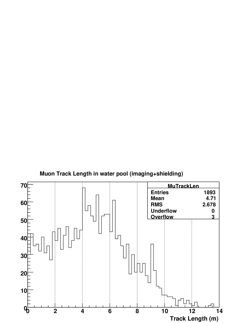
Figure 7.2: Track length of muons in the water shield for the Daya Bay Near Hall.

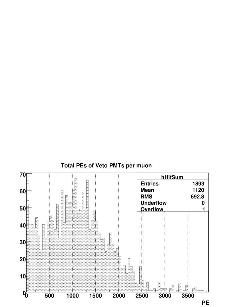
Figure 7.3: Total number of photoelectrons observed in baseline configuration in the Daya Bay Hall.

These photoelectrons are spread over an average of $\sim$130 PMTs as seen in Fig. 7.5, and the resulting distribution of photoelectrons in a single PMT is shown in Fig. 7.5. As expected the average is about 8 photoelectrons, although there is a long tail exponential tail with a slope of $\sim$26.

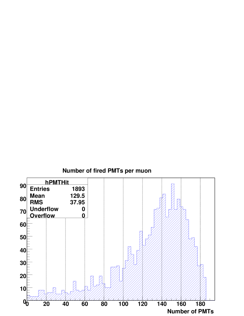
Figure 7.4: Number of phototubes hit in baseline configuration of the Day Bay Near Hall.

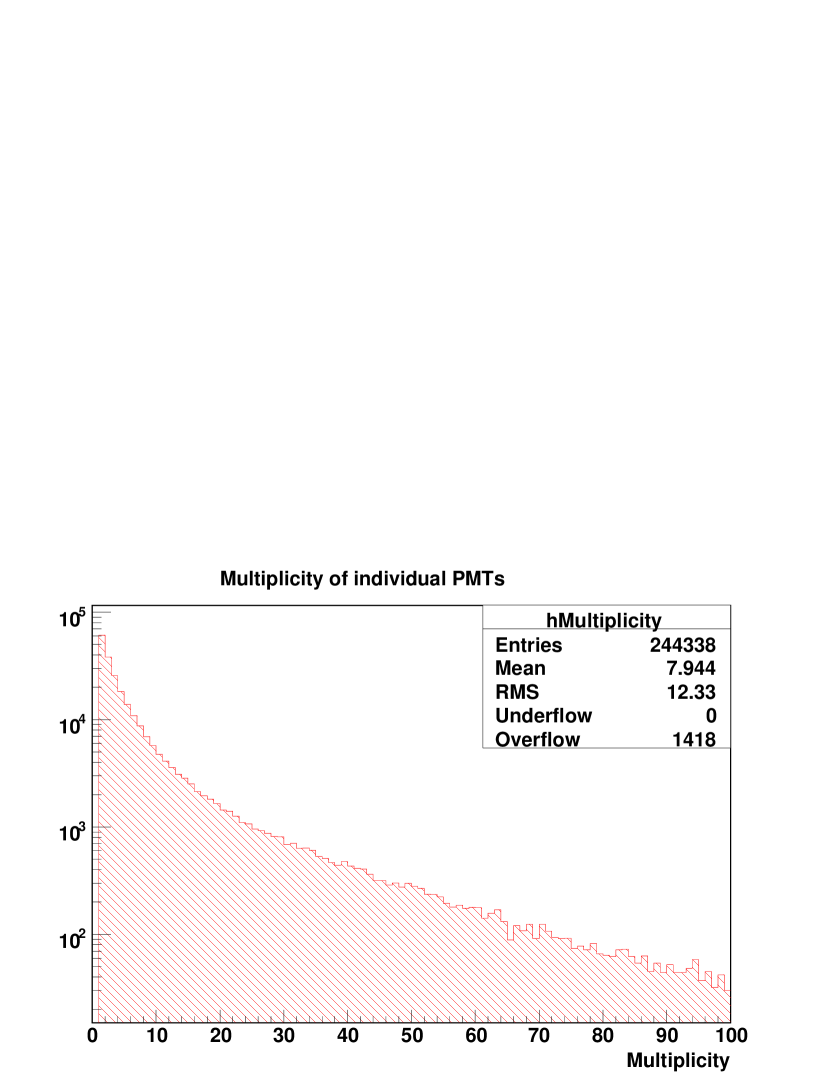
Figure 7.5: Photoelectrons observed per PMT in baseline configuration of the Daya Bay Near Hall.

Initial results on efficiency of the water shield as a function of the number of PMTs demanded are shown in Fig. 7.7. In each case a threshold number of PMTs is determined by the requirement that the deadtime due to random coincidences be $<$1%. Conservatively an effective singles rate (dark current plus radioactivity) of 50 kHz/PMT was assumed for this calculation. For the baseline configuration described above, this level was reached at a threshold of 12 PMTs, yielding an efficiency of $>$99.3% as can be seen from the black curve, labeled “K” in Fig. 7.7.

Results from three other configurations are also shown. The green curve, labeled “I” corresponds to a configuration similar to that of the baseline, but with a higher density of PMTs (1.1 m spacing instead of 1.4 m). A threshold of 17 PMTs is needed to reduce the random trigger deadtime to below 1%. At this point the efficiency is a little above 99.2%, i.e. statistically identical to that of the baseline. However it’s clear that if a higher threshold should be needed, the efficiency of this configuration holds up better than that of the baseline. The red curve, labeled “C”, corresponds to a case when PMTs are deployed on many other surfaces of the pool (at the same 1.4 m spacing). In addition to the sides and bottom of the pool, for this configuration, there is a plane of PMTs at the top of the pool looking down into it, a plane parallel to this one just above the antineutrino detectors looking up, and vertical planes abutting the antineutrino detectors (forming a “box” around the detectors) with the PMTs looking out into the pool. For this configuration, the random coincidence rate reaches 30Hz, which results in a deadtime of 0.6%, at a threshold of 17 PMTs. At this point the efficiency is about 99.6%. This configuration has clearly better performance than that of the baseline, although at the cost of twice as many PMTs and much added complication in the PMT mounting scheme. A configuration more efficient in the number of PMTs than the baseline is shown in blue, labeled “M”. This configuration has no inward-looking PMTs except near the corners of bottom of the pool. There are upward-facing PMTs above the antineutrino detectors and outward-facing PMTs on the sides of the “box” surrounding those detectors. The PMTs are spaced at 1.4 m. The “M” configuration has very similar efficiency performance to that of the baseline, but requires 25% fewer PMTs (albeit at the cost of a more complicated mounting system).

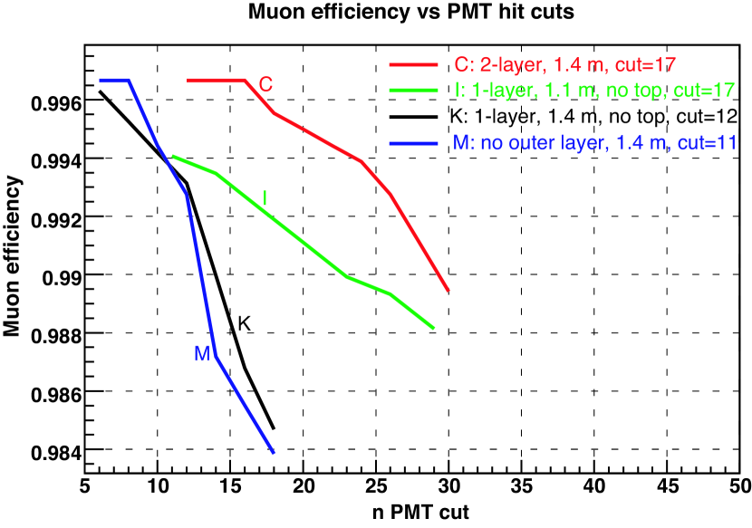
Figure 7.6: Muon efficiency of the water shield as a function of threshold (in number of PMTs hit) for four different configurations of PMTs. The black curve represents the performance of the current baseline.

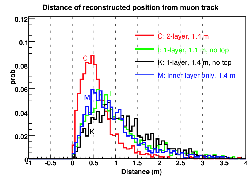
Figure 7.7: Difference between the reconstructed position and the nearest point on the actual muon trajectory for four different configurations. The black curve is for the current baseline.

An initial attempt was made to develop a position-determining algorithm. The positions of the five PMTs with earliest light are averaged to obtain an estimator of the muon position. This was tested in the same GEANT runs used to calculate efficiency. In Fig. 7.7 the difference between the calculated position and actual trajectory of the muon is plotted for the four configurations discussed above. For the baseline, the resolution averages $\sim$0.9 m. Doubling the numbers of PMTs in the same configuration doesn’t help much here. However the “M” configuration performs a little better than the baseline, and the “C” configuration with both more PMTs and more surfaces has substantially better performance.

These results on efficiency and position determination, although preliminary are extremely encouraging.

7.2.4 Water Buffer Front-End Electronics

Extrapolation of the curve in Fig. 7.5 indicates that although the number of photoelectrons per PMT has a long tail, only about 0.01% of the PMTs see more than 100 photoelectrons. Thus the performance of the antineutrino detector electronics should certainly be adequate for the water buffer readout. However the reduced dynamic range requirement may indicate that less expensive options should be considered for the pulse height measurement. In addition to the pulse height information, timing information will also be provided by the readout electronics. With 0.5 ns/bin TDCs, a timing resolution of 2 ns is readily achievable for a single PMT channel. The energy sum of the PMTs as well as the multiplicity of the struck PMTs will be used for defining the muon trigger (see Sect. 8.1.3).

7.2.5 Calibration of the Water Buffer PMTs

The gain stability and the timing of the PMTs will be monitored by a LED system identical to that for the neutrino detectors. No radioactive sources will be required.

7.2.6 Purification of the Water Buffer

We must purify the water to maintain constant water transparency and to prevent microbial growth.

We must also recirculate the water to maintain a constant relatively low temperature (15^∘C) to inhibit microbial growth and maintain the antineutrino detectors at constant temperature. Also, we must remove impurities that have leached into the water from the detector materials and wall during recirculation.

The level of purity needed to prevent growth will reduce radioactive backgrounds to well below the level where they would make detectable background in the antineutrino detectors.

7.3 Muon Tracker

The muon tracker has the job of tagging the entering muons and determining their path through the region of the antineutrino detectors. In addition, it must measure the efficiency of the water shield for muons.

Three technologies are being considered for the muon tracker. RPCs can be used on top of the water shield, but to use them in the water would require a large program of R&D on techniques of encapsulation. Water Cherenkov modules are cheap and practical to operate in the water, but would be difficult to remove from the top of the water shield when the antineutrino detectors need maintenance or have to be moved. Plastic strip scintillators can be operated either on top of the water or in it, although the latter requires developing an encapsulation scheme.

7.3.1 Resistive Plate Chambers (RPC)

The RPC is an attractive candidate tracking detector since it is economical for instrumenting large areas. Furthermore, RPCs are simple to fabricate. The manufacturing technique for both Bakelite (developed by IHEP for the BES-III detector [2]) and glass RPCs (developed for Belle [3]) are well established.

An RPC is composed of two resistive plates with gas flowing between them. High voltage is applied on the plates to produce a strong electric field in the gas. When a charged particle passes through the gas, an avalanche or a streamer is produced. The electrical signal is then registered by a pickup strip and sent to the data acquisition system. In our case, the RPCs will operate in the streamer mode.

The RPCs for the BES-III spectrometer were constructed using a new type of phenolic paper laminate developed at IHEP. The surface quality of these plates is markedly improved compared to the Bakelite plates previously used to construct RPCs. IHEP has developed a technique to control the resistivity of the laminates to any value within a range of $10^{9}\!-\!10^{13}\ \Omega\cdot$m. About 1000 bare chambers ($\sim$1500 m²) without linseed oil coating have been produced for BES-III. Tests show that the performance of this type of RPC is comparable in performance to RPCs made with linseed oil-treated Bakelite and to glass RPCs operated in streamer mode. Applying linseed oil to Bakelite is a time-consuming step in the productions, and presents a major risk factor in the long-term operation of the chambers.

The efficiency and noise rate of the BES-III RPCs have been measured. In Fig. 7.9, the efficiencies versus high voltage are shown for threshold settings between 50 and 250 mV. The efficiency as plotted does not include the dead area along the edge of the detector, but does include the dead region caused by the insulation gasket. This kind of dead area covers 1.25% of the total detection area. The efficiency of the RPC reaches plateau at 7.6 KV and rises slightly to 98% at 8.0 KV for a threshold of 150 mV. There is no obvious difference in efficiency above 8.0 KV for thresholds below 200 mV. The singles rate of the RPC shortly after production is shown in Fig. 7.9.

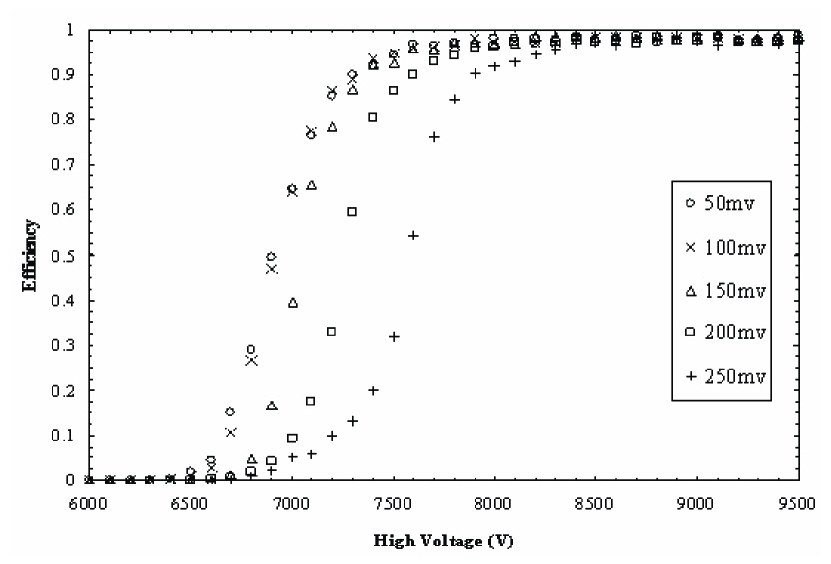
Figure 7.8: Efficiency of the BES-III RPC versus high voltage for different thresholds.

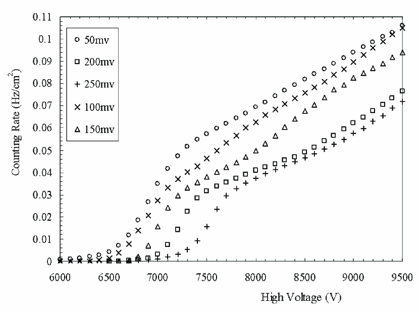
Figure 7.9: Noise rate of the BES-III RPC versus high voltage for different thresholds.

The typical singles rate at thresholds above 150 mV is $<$0.1 Hz/cm² after training. The noise rate increases significantly when the high voltage is higher than 8 kV.

In cosmic ray tests of a large sample of BES chambers, the average efficiency was 97%, and only 2 had efficiency less than 92%. Figure 7.10a shows the efficiency distribution. This efficiency was obtained with no corresponding excessive chamber noise. Figure 7.10b shows the RPCs singles rate.

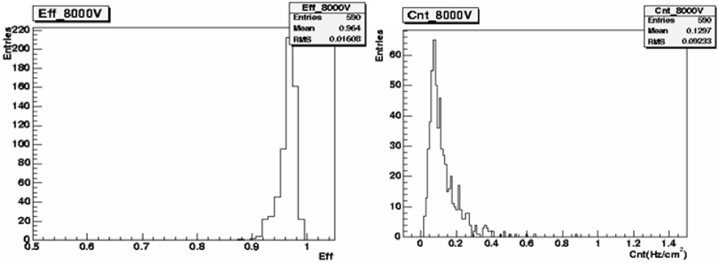
Figure 7.10: Distribution of tested RPC a) efficiencies and b) singles rates.

The most probable value was $\sim$0.08 Hz/cm² and the average was 0.13 Hz, with only 1.5% higher than 0.3 Hz/cm².

7.3.2 RPC Design

The above measurements were made with one dimensional readout RPCs. For the Daya Bay experiment, we are planning to use RPCs with readout in two dimensions in order to get both x and y-coordinates of the cosmic muons (similar in design to the BELLE RPCs [3]). Three double gap layers would be combined to form a module. The layers are electrically shielded from one another to avoid cross talk. The structure of a single such layer is shown in Fig. 7.11.

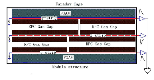
Figure 7.11: Structure for a double-gap RPC module. Three such layers are envisioned.

Plastic spacers will be used periodically to precisely maintain the gap width. These spacers are potentially a source of dead space. Therefore, within each module, spacers in different layers will be offset, resulting in no aligned dead space. Also, modules will overlap at the edges, so there will be no inter-module dead space. The double-gap design improves robustness and efficiency, at the cost of doubling the noise rate.

Bakelite modules as large as 1 m$\times$2 m are straightforward to manufacture. Two of these will be bonded together to make a single 2 m$\times$2 m unit. The chambers will be read out by strips of $\sim$14 cm dimension. Thus each unit will have 28 readout channels. With adequate module overlap and the peaked roof shown in Fig. 7.1 extending an extra 1m on all sides of the pool, it will be necessary to cover an area of 20 m$\times$18 m at the Far Hall and 20 m$\times$12 m at each of the near halls. This will require a total of 630 units for three layers, and a total of 17,640 readout strips.

Alternatively glass modules as large as 1.5 m$\times$1.5 m are easy to make and convenient to handle. They would have $\sim$19 cm-wide readout strips. These would require a total of 1092 units and 17,472 readout strips.

7.3.3 RPC Mounting

Figure 7.12 shows a candidate scheme for mounting the RPCs on a peaked roof over the water pool.

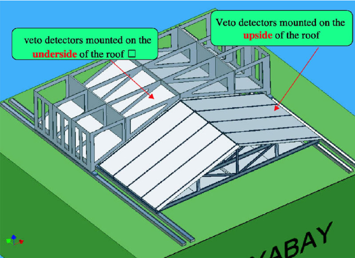
Figure 7.12: Sliding roof mount for muon tracker modules above the water pool.

The roof will be divided into two sections of different heights and the RPCs mounted in a way that allows one section to slide over or under the other.

7.3.4 RPC Performance

Taking into account inefficiencies due to dead-spaces, we expect the overall efficiency of a single layer to be at least $\varepsilon\sim$96%. If we adopt the definition of a track as hits in at least two out of three layers then the coincidence efficiency is $\varepsilon^{3}+C^{2}_{3}\varepsilon^{2}(1-\varepsilon)=0.96^{3}+3\times 0.96^{2}\times(1-0.96)=99.5$%, where $C^{2}_{3}=3$ is the binomial coefficient. Assuming a bare chamber noise rate, $r$, of 1.6 kHz/m² is achieved (consistent with twice the BES chamber measurements), a signal overlap width $\tau$, of 20 ns, and a coincidence area, $A$, of 0.25 m², the noise rate would be $C^{2}_{3}A^{2}r^{2}\tau(1$ m${}^{2}/A^{2})=3\times 1600^{2}\times 0.2\cdot 10^{-7}=0.154$ Hz/m². For the Far Hall, this gives a total accidental rate of 55 Hz and a corresponding contribution to the deadtime of 1.1% in the case that a muon signal is defined by a hit in the RPCs alone. A test of the 3 layer scenario with prototypes of the Daya Bay chambers, using a track definition of two out of three hits, found a coincidence efficiency of 99.5$\pm$0.25%, which is consistent with the calculated efficiency. The efficiency curves are shown in Fig. 7.13.

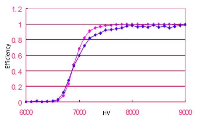
Figure 7.13: Efficiency as a function of gap voltage for the individual modules of the Daya Bay prototype RPCs (blue) and for the system when two out of three hit modules are required (red).

Initial simulation results based on measurements of radioactivity in the Aberdeen Tunnel predict singles rates from radioactivity of $\sim$650 Hz/m² and coincidence rate of 1 Hz/m², mainly from double Comptons. This corresponds to a trigger of $\sim$300 Hz in the Far Hall and a contribution to the veto deadtime of $\sim$6%.

7.3.5 RPC Front-End Electronics

The readout system consists of a readout subsystem, a threshold control subsystem, and a test subsystem. The readout system, shown in Fig. 7.14, contains a 9U VME crate located above the detector, which holds a system control module, a readout module, an I/O module, and a JTAG control module. The system clock will operate at 100 MHz.

1) Control Module

The control module receives the trigger signals (L1, Clock, Check, and Reset) from the trigger system and transmits them to the Front End Card (FECs) through the I/O modules. It also receives commands (such as setting thresholds, testing, etc.) and transmits them to the FECs. The control module is also a transceiver which transfers the FULL signal between the readout module and FECs.

2) I/O Modules

The VME crate contains several I/O modules, each of which consists of 12 I/O sockets connected by a data chain. The I/O module drives and transmits the signals of the clock and trigger to all the FEC’s, and transmits control signals between the readout module and the FECs.

3) VME Readout Modules

The readout module is responsible for all the operations relative to data readout. It not only reads and sparsifies the data from all the data chains (it can read 40 of them in parallel), constructs the sub-event data to save into the buffer, and requests the interrupt to the DAQ system to process the sub-event data, but also communicates the Full signals to the FEC’s to control the data transmission. The readout module checks and resets control signals to the trigger system. It also controls the reading and sparcifying of the FEC data, the requesting of a DAQ interrupt, and the counting and resetting of the trigger number.

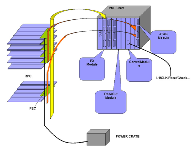
Figure 7.14: Configuration of the electronics & readout system.

4) Front-End Cards

The FECs are located on the RPC detector. Their task is to transform signals from the strips into a bit map, store the data in a buffer and wait for a trigger signal. Events with a trigger will be transmitted in a chain event buffer in the VME readout modules. Events without a trigger are cleared. Analog signals from groups of 16 strips are discriminated and the output read and stored in parallel into a 16-bit shift register, which is connected to a 16-shift daisy chain. A total of 16 FECs compose one FEC Daisy-Chain, which covers 256 strips. The data from each chain, as position information, are transferred bit-by-bit to the readout module in the VME crate through the I/O modules using differential LVDS signals. Each datum of the chain will be stored temporarily in the relative data chain buffer of the readout module. After the data sparsification, the whole data chain will be stored into the sub-event data buffer awaiting DAQ processing.

In each FEC there is also a DAC chip, which is used to generate test signals. When a test command goes to the test signal generator which resides in the system control module in the VME crate, the generator sends timing pulses to the FEC’s DAC chip through an I/O module. This chip then delivers a test signal to each channel’s comparator.

The principle of the threshold setting circuit is the same as the test circuit. The timing pulses are generated by the threshold controller in the system control module, and sent to the DAC to generate the threshold level at each of the input ports of the discriminators in the FEC.

5) JTAG Module

The JTAG module gets the FPGA setting command from the VME BUS, transforms the command into the JTAG control timing, and sends it to the FECs. Each of the JTAG modules has 12 slots on the panel of the module, enough to satisfy the requirements of the whole readout system.

6) Test System

The test system for the readout system consists of the test control module in the VME crate, and a test function generator in the FEC.

7) Threshold-Setting System

The threshold-setting system for the readout system consists of the threshold-setting control module in the VME crate, and a threshold-setting generator in the FEC.

7.3.6 Water Cherenkov Modules

As a part of the preliminary R&D for a long baseline neutrino oscillation experiment, the novel idea of a water Cherenkov calorimeter made of water tanks was investigated [4]. A water tank prototype made of PVC with dimensions 1$\times$1$\times$13 m³ was built. The inner wall of the tank is covered by Tyvek film 1070D from DuPont. At each end of the tank is a Winston cone that can collect parallel light at its focal point, where an 8-in photomultiplier is situated. The Winston cone is again made of PVC, covered by aluminum film with a protective coating. Cherenkov light produced by through-going charged particles is reflected by the Tyvek and the Al film and collected by the photomultiplier.

The light collected due to cosmic-muons is a function of the distance from the point of incidence of the muon to the phototube. Such a position dependent response of the tank is critical to its energy resolution and pattern recognition capability. Typically it is characterized by an exponential behavior of $e^{-x/\lambda}$, where $x$ is the distance of the muon event to the phototube and $\lambda$ is the characteristic parameter, often called the “effective attenuation length”. The characteristic parameter $\lambda$ depends on the water transparency, the reflectivity of the Tyvek film, and the geometry of the tank. Using trigger scintillation counters to define the muon incident location, keeping the $y$ coordinate constant, the total light collected as a function of $x$ at several locations was obtained as shown in Fig. 7.15. It can also be seen from Fig. 7.15 that, for a through-going muon entering the center of the tank, $\sim$20 photoelectrons are collected by each PMT, corresponding to a statistical determination of about 7%/$\sqrt{E(GeV)}$.

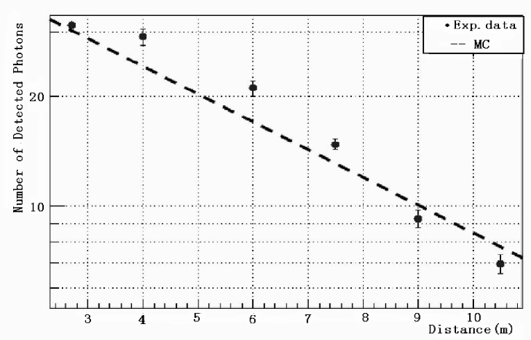
Figure 7.15: Position dependent response of the water tank to cosmic-muons. $X$ is the distance from trigger counters to the PMT at right. The line represents the Monte Carlo prediction with an effective attenuation length of 5.79 m. The measured effective attenuation length of the water tank is (5.74$\pm$0.29) m.

As discussed in Section 7.2 the Daya Bay antineutrino detector modules are to be shielded from external radiation (such as gamma-ray and cosmic-ray induced neutrons) by a $\sim$2.5-m thick water buffer. One could use modules similar to the above-mentioned Cherenkov units as the muon tracker (Fig. 7.1).

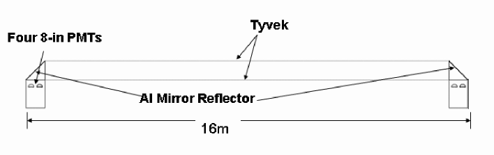
Figure 7.16: The geometry of a water Cherenkov module unit. Four 8-in PMTs are installed in each end, with an Al mirror.

Such modules have many advantages: (1) very good cosmic-ray detection efficiency (theoretically, the efficiency is close to 100%); (2) insensitivity to the natural radioactivity of Daya Bay’s rock; (3) very modest requirements on the support system because the whole detector is immersed in the water; (4) low cost because water is used as the medium.

The geometry of the water Cherenkov units located at the four sides of water pool is shown in Fig 7.16. We use four PMTs at each end to decrease the risk of failure of a unit if one PMT dies. The unique geometry of two ends reduces the optically dead region. Similar modules would be placed at the bottom of the pool.

It is possible that instead of a Tyvek lining, we may be able to rely on the reflectivity of TiO2-loaded PVC, of the sort being studied for the NOvA experiment at Fermilab. R&D on this possibility is in progress.

A modified version of the LED system discussed in Sec. 6.2 would be used for gain calibration of the WCMs.

To cover the Daya Bay and Ling Ao Near Sites and the Far Site will require 108 16 m-long units and 36 10 m-long units, with a total of 1152 8” PMTs. The WCMs will not be water-tight and will share the purification system of the water shield.

Water Cherenkov Module Performance

A GEANT4 simulation tuned to match the performance of the prototype described above was adapted to the longer modules proposed for Daya Bay. The optical parameters come from our previous MC simulation program of the prototype. Preliminary MC results are shown in Table 7.3. These show that adequate signal can be obtained from both ends of these modules for muons at any point along them.

Table 7.3: Number of photoelectrons detected in the 16 m-long water Cherenkov module with different incident positions of (vertical) muons from the Monte Carlo simulation. These modules have four PMTs on each end.

	-7m	-5m	-2m	0	2m	5m	7m
Left	9.8	23.1.	52.8	86.1	149.5	343.8	1044.9
Right	985.3	340.8	152,7	88.6	51.3	23.0	10.0

Position resolution in the direction transverse to the axis of the module will be given by its size: $\sigma_{x}=100{\rm cm}/\sqrt{12}=$ 29 cm. In the other dimension, 2 ns resolution on the end-to-end timing will contribute $\sim$32 cm to the position uncertainty. We can also use the comparison of pulse height from the two ends for determining the position. Including both methods we expect a resolution comparable or better than that in the coordinate determined by the module cross-section. For muons that traverse the water pool and hit modules on either side, these resolutions yield uncertainties of $\sim$21 cm on the position at the center of the trajectory.

Accidental rates in this system, which is essentially blind to rock radioactivity, are expected to be negligibly small.

From Table 7.3, we see it is desirable to measure signals that are $\sim$1 photoelectron to those that are several hundred photoelectrons. Thus the same electronics discussed in Sect. 7.2.4 are appropriate for use here.

7.3.7 Plastic Scintillator Strips

Plastic scintillator strips serve as a backup option for both the top and in-water tracking systems. For both purposes we propose to use the extruded plastic scintillator strip technology developed by MINOS, OPERA and other previous experiments. The parameters of this system are shown in Table  7.4.

Name	value	unit
number of strips	5304
length of strip	5.25	m
width of strip	0.2	m
thickness of strip	1	cm
fibers/strip	5
length of fiber	7.25	m
diameter of fiber	1	mm
strips/module	6
modules (full/top only)	884/295
phototubes (full/top only)	1768/530

Table 7.4: Parameters of scintillator strip detectors

If the scintillators are used for the entire muon tracker system they will be set back from the walls and floor of the pool by 50 cm to allow attenuation of the gammas from rock radioactivity. For a similar reason they will be mounted 50 cm below the top of the pool. There will be two orthogonal layers on each wall, the floor and the top. In the case where only the top is to be covered by scintillator strips, they would be arrayed in the manner described above for the RPCs, i.e. there would be three layers mounted on the sliding roof. In this case a triple coincidence could be demanded if made necessary by the random rates.

Scintillator Strip Design

Almost all the scintillators will be of the same type: 5.25 m$\times$0.2 m$\times$0.01 m extruded polystyrene, co-extruded with a coating of TiO2-doped PVC. Five 1 mm Kuraray Y-11(200) S-type wavelength-shifting fibers will be glued into 2 mm deep $\times$ 1.6 mm wide grooves in the plastic using optical glue [6]. Six such scintillators will be placed in a single frame and read out as one 1.2 m-wide unit. Figure 7.17 shows the cross section of one scintillator.

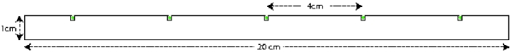
Figure 7.17: Cross-section of a single scintillator strip.

Scintillator Strip Photoreadout

A 1$\frac{1}{8}$-inch photomultiplier tube such as a Hamamatsu R6095 or Electron Tubes 9128B will be used to read out 30 fibers on each end of the six-scintillator module. The PMTs will be run at positive HV, via a system similar to that discussed in Sect. 5.4.4. Calibration will be via thin-film ²⁴¹Am sources placed near the ends of the scintillators. The sources provide $\sim$400 Hz of $\sim$0.5 MeV signals.

Counter Housing and Support

Above the water, the counters will be mounted on a simple system of strongbacks supported by the sliding roof. In the water, the requirements for deployment are much more demanding. The six scintillator strips will be housed in an RPVC extruded box, shown in Fig. 7.19. The box ends are closed by custom manifolds that contain the fiber ends which are dressed to have an equal length of $\sim$90 cm. The fibers will be routed through a molded cookie, gathered into single bundle and conducted in a PVC pipe through the water into a separate small enclosure containing the PMT/base assembly. Figure 7.19 shows the module end, routing cookie and PMT containment.

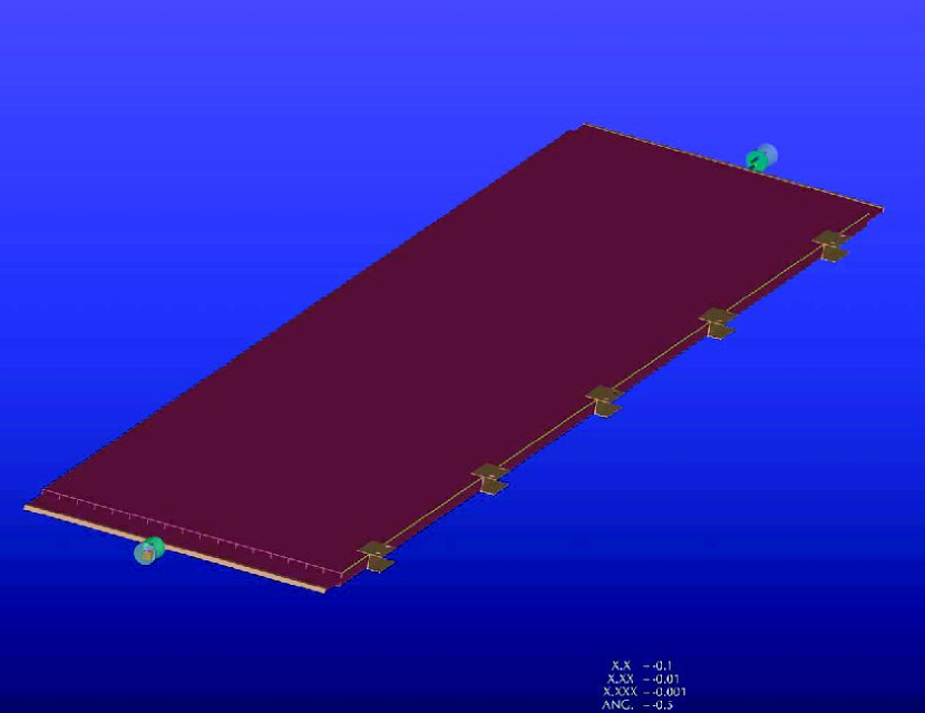
Figure 7.18: Extruded container for six-scintillator module

.

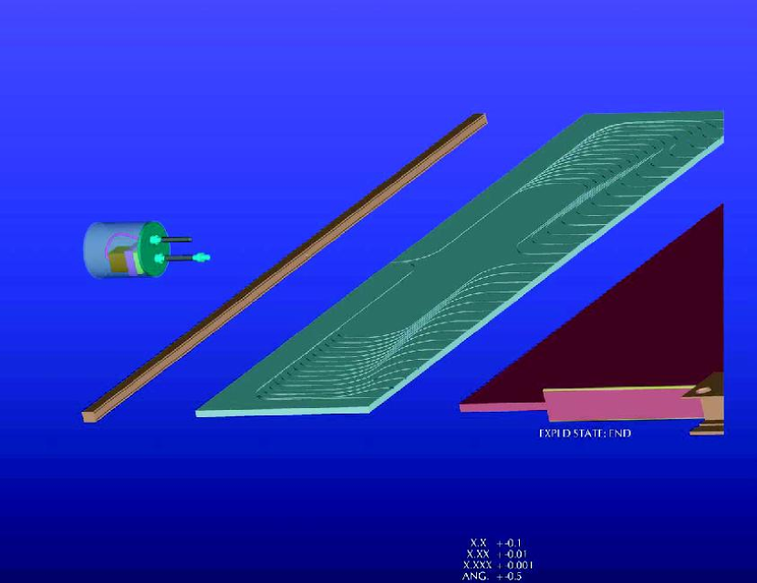
Figure 7.19: Exploded view of the end of the scintillator housing module showing routing of fibers, PMT containment, and other details.

The scintillator housings will be supported by a steel frame in a manner similar to the H-clip technique used by MINOS [7], although our version, shown in Fig. 7.21, will be made of RPVC. It will be glued onto the module housing and fixed to the frame with two hole-drilling screws or blind rivets. Figure 7.21 shows the support scheme for the side walls of the scintillator system.

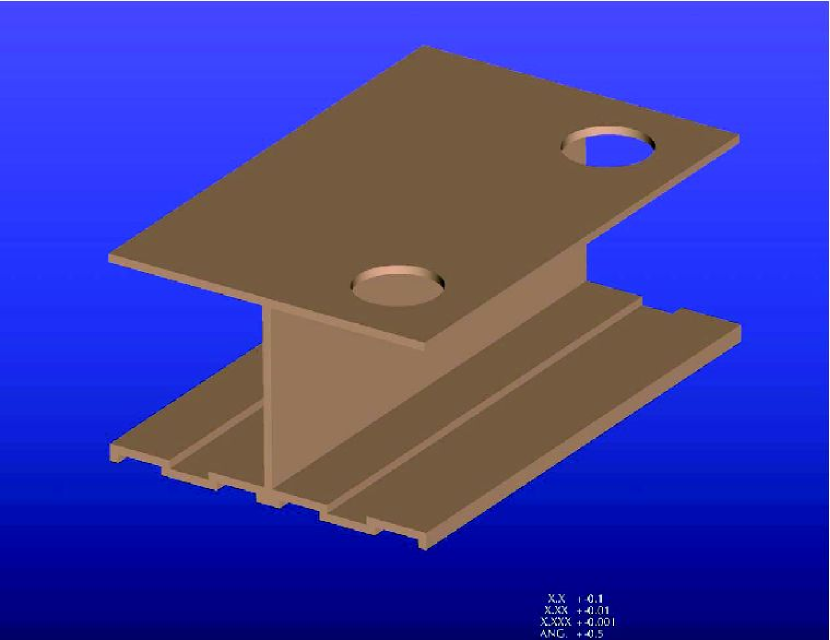
Figure 7.20: H-clip to hold the scintillator housing.

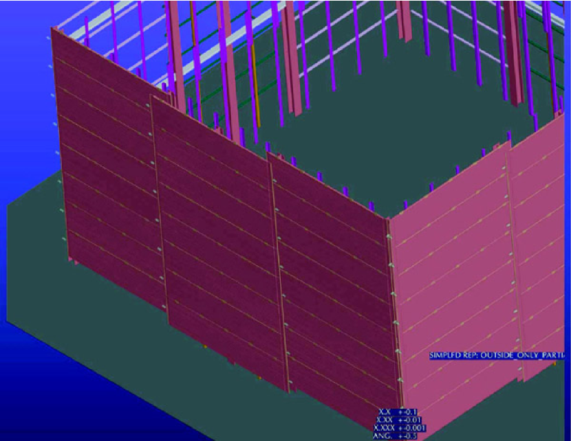
Figure 7.21: Side walls of the scintillator strip system partially assembled.

7.3.8 Scintillator Strip Performance

We base our expectation of performance on that of the prototype OPERA target tracker scintillators [8]. Figure 7.22 shows the yield of photoelectrons versus distance to the photomultiplier tubes.

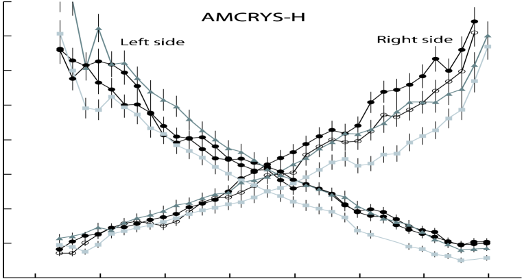
Figure 7.22: Number of photoelectrons detected on each side of several AMCRYS-H plastic scintillator strips versus the distance to the photomultipliers (from Dracos et al.).

Note that our counters are only a little longer than 5 m, a point at which the OPERA strips yield about 6 p.e.

The OPERA strips are 26 mm wide by 10.6 mm thick. Our strips are 200 mm wide by 10 mm thick. The MINOS GEANT3 Monte Carlo was adapted to compare the two cases. For collection into the wavelength-shifting fibers, the fraction of OPERA performance for 4, 5, and 6 fibers per 20 cm is 0.74, 0.89, and 1.02 respectively. OPERA uses Hamamatsu H7546-M64 PMTs, which have a photocathode efficiency about 80% as high as either of the single-anode tube we are planning to use. Thus any of the 4–6 fiber cases should achieve performance similar to that of OPERA. For estimation purposes we choose 5 fibers, which nominally should give 1.15 times OPERA performance in our system. The single photoelectron pulse height distribution will reduce the effective number of photoelectrons by a factor of (1 + the variance of the distribution). With PMTs of the type discussed, this will result in an inefficiency of $\sim$0.6% in the worst case (hit at one end of the counter). An upper limit on the position resolution is given by the granularity of the counters: $\sigma_{x}=120{\rm cm}/\sqrt{12}\approx 35\,{\rm cm}$. For a muon that hits two sides of the pool, the resolution on the position at the center of its trajectory through the pool will be $\sim$ 25 cm. End-to-end timing and pulse height are expected to improve this. A timing resolution of 1 ns will contribute $\sim$15 cm to the resolution along the counter and $\sim$11 cm to the resolution at the center of the trajectory for through-going muons.

Plastic scintillators are sensitive to the ambient radioactivity from rock. Tests of these rates were carried out with a scintillator telescope in the Aberdeen Tunnel in Hong Kong [9], which has similar granite to that of Daya Bay. These indicate that the true coincidence rate of two 1cm layers at a threshold of 0.5 MeV would be $\sim$7 Hz/m². For the relevant active area of the top of the Far Hall water pool, this gives an overall rate of $\sim$1800 Hz. If the top scintillator array alone were used as a 200 $\mu$s veto, it would give an unacceptable random veto deadtime. However, for through-going muons that could be required to register as well on the side or bottom of the pool, the random veto rate would be reduced to a negligible level (with the shielding from 50 cm of water, the coincidence rate in scintillators in the pool would be expected to be only 0.7 Hz/m², so 180 Hz on the bottom which is the worst case). Since the background from stopping muons is extremely small, scintillators seem acceptable in either or both roles.

7.3.9 Scintillator Strip Front-End Electronics

Once again, the electronics and readout discussed in Sect. 7.2.4 would be adequate for this system. However since it is not necessary to measure energies above a few MeV, a smaller dynamic range would be acceptable. Whether it is worth it to develop separate electronics for this case is under study. In any case the readout would be similar to that discussed in Sect. 5.5.

8 Trigger and Data Acquisition System

The trigger event selection and estimated rates are presented, along with the timing synchronization between all of the electronics elements. The processing of the trigger data from the front-end modules through data storage is discussed, along with the detector control system.

8.1 The Trigger System

The trigger system of the Daya Bay experiment makes trigger decisions for the antineutrino and muon detectors to select neutrino-like events, muon-related events, periodic trigger events and calibration trigger events. The following sections will describe the requirements and technical baseline for the trigger system.

8.1.1 Requirements

The signature of a neutrino interaction in the Daya Bay antineutrino detectors is a prompt positron with a minimum energy of 1.022 MeV plus a delayed neutron. About 90% of the neutrons are captured on Gadolinium, giving rise to an 8 MeV gamma cascade with a capture time of 28 $\mu$s. The main backgrounds to the signal in the antineutrino detectors are fast neutrons produced by cosmic muon interactions in the rock, ⁸He/⁹Li, which are also produced by cosmic muons and accidental coincidences between natural radioactivity and neutrons produced by cosmic muons. All three major backgrounds are related to cosmic muons. The following are the main trigger requirements imposed by the physics goals of the Daya Bay experiment:

1. Energy threshold: The trigger is required to independently trigger on both the prompt positron signal of 1.022 MeV and the delayed neutron capture event with a photon cascade of $\approx$8 MeV with very high efficiency. The threshold level of the trigger is set at 0.7 MeV. This level corresponds to the minimum visible positron energy adjusted for a $3\sigma$ energy resolution effect. This low threshold requirement fulfils two trigger goals. For the neutrino signal, it allows the DAQ to record all prompt positron signals produced from the neutrino interactions, enabling a complete energy spectrum analysis that increases the sensitivity to $\theta_{13}$. For background, it allows the DAQ to register enough uncorrelated background events due to either PMT dark noise or low energy natural radioactivity to enable a detailed analysis of backgrounds offline.

2. Trigger efficiency: In the early stages of the experiment, the trigger efficiency is required to be as high as possible for signal and background, provided that the event rate is still acceptable and will not introduce any dead time. After an accurate characterization of all the backgrounds present has been achieved, the trigger system can then be modified to have more powerful background rejection without any efficiency loss for the signal. To measure the efficiency variation, the system should provide a random periodic trigger with no requirement on the energy threshold at trigger level. A precise spectrum analysis also requires an energy-independent trigger efficiency for the whole signal energy region.

3. Time stamp: Since neutrino events are constructed offline from the time correlation between the prompt positron signal and the neutron capture signal, each front-end (FEE), DAQ and trigger unit must be able to independently time-stamp events with an accuracy better than 1 $\mu$s. The trigger boards should provide an independent local system clock and a global time-stamp to all the DAQ and FEE readout boards in the same crate. The trigger boards in each DAQ crate will receive timing signals from a global GPS based master clock system as described in Section 8.2. Events recorded by the antineutrino detectors and muon systems can thus be accurately associated in time offline using the time-stamp.

4. Flexibility: The system must be able to easily implement various trigger algorithms using the same basic trigger board design for different purposes such as

   1. Using different energy thresholds to adapt to the possible aging effect of liquid scintillator, or for triggering on calibration source events which have lower energy signatures.

   2. Using different hit multiplicities to increase the rejection power due to the uncorrelated low energy background and for special calibration triggers.

   3. Implementing different pattern recognition for triggering on muon signals in the different muon systems.

   4. Using an OR of the trigger decision of different trigger algorithms to provide a cross-check and cross-calibration of the different algorithms as well as a redundancy to achieve a high trigger efficiency.

5. Independence: Separate trigger system modules should be used for each of the antineutrino detectors, and the muon systems. This is to reduce the possibility of introducing correlations between triggers from different detector systems caused by a common hardware failure.

8.1.2 The Antineutrino Detector Trigger System

Neutrino interactions inside a detector module deposit an energy signature that is converted to optical photons which are then detected by a number of the PMTs mounted on the inside of the detector module. Two different types of triggers can be devised to observe this interaction:

1. An energy sum trigger.

2. A multiplicity trigger.

In addition to neutrino interaction triggers, the antineutrino detector trigger system needs to implement several other types of triggers for calibration and monitoring:

1. Calibration triggers of which there are several types:

   1. Triggers generated by the LED pulsing system that routinely monitors PMT gains and timing.

   2. Triggers generated by the light sources periodically lowered into the detector volume to monitor spatial uniformity of the detector response and the light attenuation.

   3. Specialty energy and multiplicity triggers used to test detector response using radioactive sources

2. A periodic trigger to monitor detector stability and random backgrounds.

3. An energy sum and/or multiplicity trigger (with looser threshold and multiplicity requirements) generated in individual antineutrino detector modules which is initiated by a delay trigger from the muon system. This trigger records events to study muon induced backgrounds. This trigger should be able to operate in both tag and veto modes.

A VME module with on-board Field Programmable Gate Arrays (FPGA)s is used to implement the antineutrino detector trigger scheme outlined in Fig. 8.1 based on experiences gained at the Palo Verde [1] and KamLAND experiments.

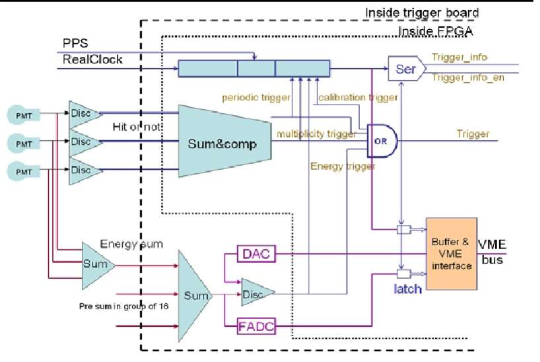
Figure 8.1: A simplified trigger scheme.

We use an OR of both an energy sum and a multiplicity trigger to signal the presence of neutrino interactions in the antineutrino detector. These two triggers provide a cross-check and cross-calibration of each other.

The multiplicity trigger is implemented with FPGAs which can perform complicated pattern recognition in a very short time. FPGAs are flexible and can be easily reprogrammed should trigger conditions change. In addition, different pattern recognition software can be downloaded remotely during special calibration runs, such as might be needed for detector calibration with sources. The signal from different PMTs is compared with the threshold on on-board discriminators in the front-end readout cards as described in Section 5.5. The output of the PMT discriminators are input into the trigger module FPGA which performs clustering and pattern recognition and generates the multiplicity trigger decision. The dark current rate of the low activity antineutrino detector PMTs is typically around 5 kHz at 15^∘ C. For a detector with $N$ total PMTs, a dark current rate of $f$ Hz, and an integration time of $\tau$ ns, the trigger rate $R$ given a multiplicity threshold $m$ is

$$R=\frac{1}{\tau}\sum_{i=m}^{N}iC_{N}^{i}(f\tau)^{i}(1-f\tau)^{N-i},\ \ \ f\tau<<1$$ (49)

where $C_{N}^{i}$ are the binomial coefficients.

To be conservative, we assume a PMT dark current rate of 50 kHz when estimating the dark current event rate from the multiplicity trigger. For the multiplicity trigger, an integration window of 100 ns will be used for the central detector PMTs. The dark current rate calculated using Eq. 49 as a function of the number of PMT coincidences is shown in Fig. 8.2.

Figure 8.2: Calculated trigger rates caused by PMT dark current as a function of the multiplicity threshold. The maximum number of PMTs is 200, the PMT dark current rate used is 50k with a 100 ns integration window.

At a multiplicity of 10 PMTs, the total trigger rate would be of order 1 Hz with a 100 ns integration window.

The energy sum trigger is the sum of charges from all PMTs obtained from the front-end readout boards with a 100 ns integrator and discriminator. The threshold of the discriminator is generated with a programmable DAC which can be set via the VME backplane bus. The energy sum is digitized using a 200 MHz flash ADC (FADC) on the trigger module. We plan to have an energy trigger threshold of 0.7 MeV or less to be compatible with the positron energy of 1.022 MeV within 3$\sigma$ of the energy resolution. At such low energy thresholds, the trigger will be dominated by two types of background: One is natural radioactivity originating in the surrounding environment which is less than 50 Hz as shown in a Monte Carlo simulation in Section 3.4.4, and the other is from cosmic muons (negligible at the far site). At this threshold, the energy sum trigger rate from the PMT dark current with a 100 ns integration window is negligible.

Tagging antineutrino interactions in the detector requires measuring the time-correlation between different trigger events. The time-correlation will be performed offline, therefore each triggered event needs to be individually timestamped with an accuracy of order of microseconds or better. It may become necessary to have a correlated event trigger in the case the background rate is too high.

A periodic trigger to monitor the PMT dark-current, the cosmic ray background, and detector stability will be included.

8.1.3 The Muon Trigger System

The muon system will utilize three separate trigger and DAQ VME crates, one for each of the muon detector systems: The water Cherenkov detector, the RPC system and the muon tracker system (scintillators or water trackers).

The presence of a muon which goes through the water Cherenkov detector can be tagged with energy sum and multiplicity triggers using a similar scheme and hardware modules as used for the antineutrino detector. In addition, a more complicated pattern recognition scheme using localized energy and multiplicity information may be used. The trigger rate in the water Cherenkov detector is dominated by the cosmic muon rate which is $<$15 Hz in the far hall and $<$300 Hz in the near halls (see Table 8.1). In addition to the water pool Cherenkov detector trigger, muons will be tagged by a system of RPCs and either water tracker modules or double layers of scintillator strips.

The FPGA logic used for the RPC and scintillator strip detectors forms muon “stubs” from coincident hits in two overlapping layers of scintillator or two out of three layers of RPC. Although the readout electronics of RPC is very different from that of the PMT, the trigger board can still be similar to the other trigger boards. As we discussed before, each FEC of RPC readout electronics can provide a fast OR signal of 16 channels for the trigger. All the fast OR signals will be fed into the trigger board for further decision by FPGA chips. The principal logic is to choose those events with hits in two out of three layers within a time window of 20 ns in a localized region of typically 0.25 m². Since the noise rate of a double gap RPC is estimated to be about 1.6 kHz/m² (consistent with twice the BES single gap chamber rates), the false trigger rate from noise can then be controlled to be less than 50 Hz in such a scheme. The coincidence rate in the RPC system due to radioactivity is estimated to be 1 Hz/m² obtained from simulation results based on measurements in the Aberdeen tunnel (see Section 7.3.4). This corresponds to a radioactivity trigger rate of about 360 Hz in the far hall.

For the water tracker modules, we need three types of triggers:

1. an AND of the two ends with a threshold of approximately 3 p.e. on each end.

2. A prescaled single ended trigger with a lower threshold.

3. The energy sum of the two ends with a threshold of $\sim$ 20 p.e.

The antineutrino detector trigger board can be used to implement the trigger schemes for the water tracker. The fake trigger rates from radioactivity in the water tracker modules is expected to be negligible.

An alternative to the water tracker modules discussed above, two layers of scintillator strips in the water pool can be used as described in Section 7. The 0.5 m of water between the water pool walls and the scintillator strips provides some shielding from radioactivity in the rock which generates a rate of 180 Hz of background in the largest plane (bottom of the far detector). The scintillator PMTs noise rate is $<$2 kHz at 15^∘ C. Requiring a coincidence of two hits in overlapping layers with a 100 ns integration window reduces the fake trigger rate from the scintillator strip PMT noise to a negligible level. In principal, the same trigger module design can be used for both RPCs and scintillator strips with different FPGA software to handle the stub formation in the different geometries.

The global muon trigger decision is an OR of the three muon detector trigger systems: RPC, water Cherenkov and muon tracker. The muon trigger decision may be used to launch a higher level delay trigger looking for activity inside the antineutrino detector at lower thresholds and/or multiplicities for background studies.

8.2 The Timing System

The design of the trigger and DAQ system is such that each antineutrino detector and muon detector system has independent DAQ and trigger modules. In this design it is necessary to synchronize the data from the individual DAQ and trigger systems offline. This is particularly important for tagging and understanding the backgrounds from cosmic muons. A single cosmic muon candidate will be reconstructed offline from data originating in three independent systems: the water Cherenkov pool, muon tracker and RPC tracker. Cosmic muon candidates reconstructed in the muon detector systems have to then be time correlated with activity in the antineutrino detector to study muon induced backgrounds. To this end, the Daya Bay timing system is required to provide a global time reference to the entire experiment, including the trigger, DAQ, and front-end boards for each module (LS, water Cherenkov, and tracker) at each site. By providing accurate time-stamps to all components various systematic problems can easily be diagnosed. For instance, common trigger bias, firmware failure, and dead time can all be tracked by looking for time-stamp disagreements in the data output from each component. Furthermore, by having multiple sites synchronized to the same time reference, it will be possible to identify physical phenomena such as supernova bursts or large cosmic-ray air showers.

The timing system can be conceptually divided into four subsystems: the (central) master clock, the local (site) clock, the timing control board, and the timing signal fanout.

8.2.1 Timing Master Clock

The global timing reference can easily be provided by a GPS (Global Positioning System) receiver to provide a UTC (Universal Coordinated Time) reference. Commercially-available units are typically accurate to better than 200 ns relative to UTC [2, 3].

This GPS receiver can be placed either at one of the detector sites (most conveniently the mid hall) or in a surface control building. A master clock generator will broadcast the time information to all detector sites. If the master clock is located underground, the GPS antenna may require an optical fiber connection to the surface, which again is commercially available. One such possibility is illustrated in Fig. 8.3

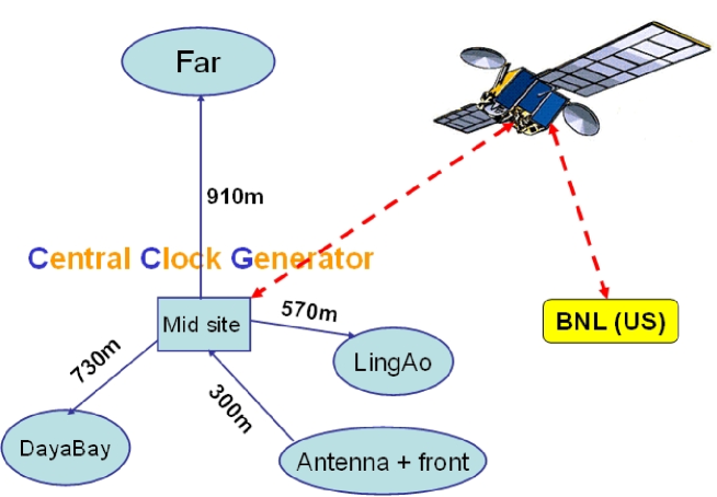
Figure 8.3: Schematic layout of the global clock.

The master clock will generate a time reference signal consisting of a 10 MHz clock signal, a PPS (Pulse Per Second) signal, and a date and time. These signals can be encoded onto a one-way fiber optic link to be carried to each of the detector halls where they are then fanned-out to individual trigger boards as shown in Fig. 8.4

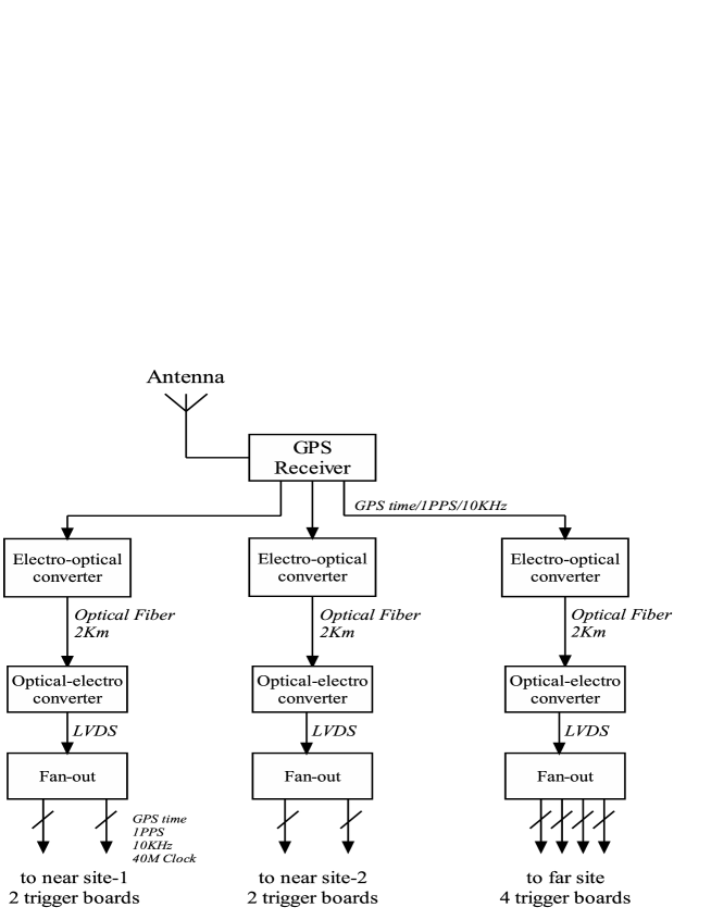
Figure 8.4: Block diagram of the Daya Bay clock system.

Additionally, the GPS receiver will be used to synchronize a local computer. This computer can then be used as a Tier-1 network time protocol (NTP) peer for all experiment computers, in particular the DAQ,

Each site will receive the signals from the master clock and use them to synchronize a quartz crystal oscillator via a phase-locked loop. This local clock can then be used as the time reference for that site.

This method allows each site to operate independently of the master clock during commissioning or in the case of hardware failure, but in normal operation provides good time reference. This clock could be used to multiply the 10 MHz time reference to the 40 MHz and 100 MHz required for the front ends. This clock will reproduce the PPS, and 10 (or 40/100) MHz signals and supply them to the timing control board.

8.2.2 Timing Control Board

The timing control board will act to control the local clock operations (i.e. to slave it to the master clock or let it run freely) and to generate any timing signals required by the trigger, DAQ, or front end that need to be synchronously delivered. Typical examples include buffer swap signals, run start/stop markers, and electronic calibration triggers. In addition, this board could be used to generate pulses used by optical calibration sources. This board would be interfaced to the detector control computers.

8.2.3 Timing Signal Fanout

The signals from the timing control board need to be delivered to the individual detector components: every FEE board, DAQ board, and trigger unit. This will allow each component to independently time-stamp events at the level of 25 ns.

This fanout system could work, for example, by encoding various signals by encoding them on a serial bus, such as HOTLink. The trigger board in each FEE and DAQ VME crate could then receive the serial signal and distribute it via the crate backplane. The crate backplanes will then carry the 40 MHz clock (100 MHz clock for RPCs), the PPS signal (to reset the clock counters), and the other timing signals (run start/stop marker, calibration, etc).

Individual components of the trigger, DAQ, and front end can employ counters and latches to count seconds since start of run and clock ticks since start of second. These will provide sufficient data to assemble events and debug the output data streams.

8.3 The Data Acquisition System

The data acquisition (DAQ) system is used to:

1. Read data from the front-end electronics.

2. Concatenate data fragments from all FEE readout into a complete event.

3. Perform fast online processing and event reconstruction for online monitoring and final trigger decisions.

4. Record event data on archival storage.

A brief review of the DAQ design requirements is followed by a discussion of the system architecture, DAQ software, and detector control and monitoring system.

8.3.1 Requirements

The Daya Bay DAQ system requirements are listed in Table 8.1.

		Trigger Rates (Hz)					data rate
Detector	Description	DB	LA	Far	Occ	Ch size	(kB/s)
$\bar{\nu}$ module	cosmic-$\mu$	$36\times 2$	$22\times 2$	$1.2\times 4$	100%	$228\times 64$ bits	217
	Rad.	$50.0\times 2$	$50.0\times 2$	$50.0\times 4$			730
RPC	Rad. & Noise	260	260	415	10%	$5040/7560\times 1$ bit	72
	cosmic-$\mu$	186	117	10.5			20
Pool	cosmic-$\mu$	250	160	13.6	50%	$252/340$ $\times 64$ bits	437
$\mu$-tracker	cosmic-$\mu$	1390	819	57.8	100%	$8\times 64$ bits	145
site totals	(kB/s)	683	500	436			1620

Table 8.1: Summary of data rate estimations. kB/s = 1000 bytes per second. The total data throughput rate for all 3 sites is estimated to be 1620 kB/s. The trigger rate for the central detector has substantial components from natural radioactivity and from muons. The trigger rate in the RPCs has, in addition, some trigger rate from noise. The trigger rate in the water pool and $\mu$-tracker comes predominantly from muons.

1. Architecture requirements: The architecture requires separate DAQ systems for the three detector sites. Each antineutrino detector module will have an independent VME readout crate that contains the trigger and DAQ modules. In addition, the water Cherenkov detector and muon tracking detectors will also have their own VME readout crates. The trigger and DAQ for the antineutrino and muon detector modules are kept separate to minimize correlations between them. The DAQ run-control is designed to be operated both locally in the detector hall during commissioning and remotely in the control room. In addition, run-control will enable independent operation of individual antineutrino and muon detector modules.

2. Event rates The trigger event rates at the Daya Bay, Ling Ao and Far site from various sources are summarized in Table 8.1. The rate of cosmic muons coming through the top of a detector are calculated using Table 3.4. To turn this into a volumetric rate, we use a MC simulation to calculate the ratio of muon rates entering the top to all muons entering the detector’s volume. The total rates from cosmic muons in the different different systems are shown in Table 8.1. At the far site, the trigger rates in the central detectors are dominated by natural radioactivity ($<$50 Hz/detector) and at the near sites both cosmic and natural radioactivity contribute.

   The trigger rate in the water Cerenkov pool is dominated by the cosmic muon rate, the singles rate from PMT noise, gammas and fast neutron backgrounds are negligible.

   The RPC noise rates are taken from the BES chamber measurements in Section 7.3.4. We scale the BES noise rates by a factor of 2 to account for the different geometry of the Daya Bay RPC modules (3 double gap layers). This increases the coincidence rate due to RPC noise by a factor of 4. The singles rates shown in Table 8.1 are the sum of the noise and natural radioactivity rates in the RPC systems at the various sites.

   For the purposes of calculating the overall data throughput for the muon tracker modules, each module is treated as an independent detector and the muon rate through each module is assumed to be its “trigger rate”. The occupancy is 100% but only 8 channels are read out. In reality of course muons will tend to hit multiple modules in one full-detector trigger but the entire detector will not be read out. In the end the two methods simply trade trigger rate for # of hit channels and the results should be the same.

   While the trigger rate in the antineutrino detectors at each site is of order a few 100 Hz, an OR of the three muon trigger systems could produce a maximum trigger rate of $<$1 kHz. The Daya Bay trigger and DAQ system will be designed to handle a maximum event rate of 1 kHz. In addition, to trigger on the correlated neutrino and fast neutron signals in the antineutrino detector, the DAQ needs to be able to acquire events that occur 1 $\mu$s or more apart.

3. Bandwidth

   The maximum number of electronics channels for the antineutrino detectors, water Cherenkov pool, and muon tracker PMTs at the far site is estimated to be at most 2000 channels as shown in Table 8.2.

   Detector Option	Geometry	Approximate number of channels
   PMT channels
   Scint tracker	2 layers
   strip module	side/bottom
   1.2 m $\times$ 5.25 m	water pool	$\sim 530$
   OR
   Water tracker	8 PMTs	$\sim 450$
   modules	per module
   1 m $\times$ 16 m module	side/bottom
   Water Cherenkov	1 PMT/2 m2
   pool	4 sides/bottom	$\sim 350$
   Antineutrino detector	4 modules	896
   Total PMT channels		$\sim 1900$
   RPC channels
   RPC on top	3 layers of
   of water pool	double gap
   2 m $\times$ 2 m module	modules	7560

   Table 8.2: Estimated number of readout channels from various detector systems at the far site.

   We assume that the largest data block needed for each PMT channel is 64 bits or less, provided waveform digitization is not used, the breakdown of the channel data block could be as follows:
   Address : 12 bits
   Timing(TDC+local time): 32 bits
   FADC : 14 bits
   For the RPC readout its 1bit/channel + header (12bits) + global time-stamp (64bits) = 1 kBytes maximum.

   Assuming zero suppression, and maximum occupancy numbers of 10% for the RPC system, 100% for 1 out of the 4 antineutrino detectors, 10% for the water tracker and 50% for the water Cherenkov (with reflecting surfaces), we estimate the maximum event size at the far will not exceed 10 kBytes/event including DAQ/Trigger header words and global time-stamps. The event sizes at the near sites are smaller than the far site due to a smaller number of channels. The expected data throughput from each site is estimated by combining the number of readout channels with the trigger rates and occupancies as shown in Table 8.1. The site totals in Table 8.1 do not include global header words, trigger words and time-stamps which add a small overhead. Therefore, we estimate that the expected data throughput rate is $<$1 MBytes/second/site. If waveform digitization is used for the PMTs, this could increase the maximum desired data throughput by an order of magnitude to $<$10 MBytes/second/site.

4. Dead-time: The DAQ is required to have a negligible readout dead-time ($<$0.5%). This requires fast online memory buffers that can hold multiple detector readout snapshots while the highest level DAQ CPUs perform online processing and final trigger decisions and transfer to permanent storage. It may also require some low level pipelines at the level of the PMT FADCs.

8.3.2 The DAQ System Architecture

The main task of the DAQ system is to record antineutrino candidate events observed in the antineutrino detectors. In order to understand the background, other types of events are also recorded, such as cosmic muon events, low energy radiative backgrounds… etc. Therefore, the DAQ must record data from the antineutrino and muon detectors (RPCs, water Cherenkov and Tracker), with precise timing information. Offline analysis will use timing information between continuous events in the antineutrino detector and in both the muon and antineutrino detectors to select antineutrino events from correlated signals or study the muon related background in the antineutrino detectors.

The DAQ architecture design is a multi-level system using advanced commercial computer and network technology as shown in Fig. 8.5.

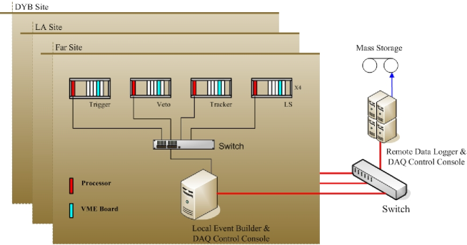
Figure 8.5: Block diagram of data acquisition system.

There should be three sets of DAQ systems: one for each of the three detector sites. The DAQ system levels shown in Fig. 8.5 are as follows:

1. VME front-ends: The lowest level is the VME based front-end readout system. Each VME crate is responsible for one detector or muon system. Each module of the antineutrino detector will have its own independent VME crate. Therefore, The lowest level VME readout system of the far detector hall will consist of the trigger boards for each system, the front-end readout boards from three muon systems, and the four antineutrino detector readout boards. All readout boards are expected to be 9U VME boards.

   The Far and Near detector halls, will have the same DAQ architecture but with different number of VME readout crates to accommodate the different number of readout channels in the Far/Near halls. Each VME crate holds a VME system controller, some front-end readout (FEE) modules and at least one trigger module which supplies the clock signals via the VME backplane to the FEE modules. The VME processor, an embedded single board computer, is used to collect, preprocess, and transfer data. The processor can read data from a FEE board via D8/D16/D32/MBLT 64 transfer mode, allowing a transfer rate up to 80 MB/s per crate which is sufficient to meet the bandwidth requirement. All readout crates of the entire DAQ system at a single site are connected via a fast asynchronous Ethernet switch to a single local event builder computer.

2. Event Builder and DAQ control: At each site an Event Builder computer collects the data from the different VME crates for the different detectors and concatenates the FEE readout to form single antineutrino or muon events. The data stream flow can work in two ways, depending on the requirements of offline analysis. One scheme is to send muon events and antineutrino events out into one data stream on the readout computer. Another scheme is that each type of sub-event, muon events, or antineutrino events, have a different data stream and will be recorded as separate data files in permanent storage. The second scheme is simpler from a DAQ design viewpoint and complies with the DAQ system design principal of keeping each detector system completely independent for both hardware and software. The Event Builder computer at each site also allows for local operation and testing of the DAQ system.

3. Data Storage and Logging:

   Data from the Event Builder computer at each site are sent via fast optical fiber link through a dedicated switch at a single surface location where it is then transferred to local hard disk arrays. The hard disk arrays act as a buffer to the remote data archival storage or as a large data cache for possible further online processing. Each day will produce about 0.6 Terabyte of data that needs to be archived. Although implementation of data logging has not yet been finalized, there are two obvious options:

   1. Set up a high bandwidth network link between Daya Bay and the Chinese University of Hong Kong, China, and distribute the data via the GRID (high bandwidth computing network and data distribution applications for high energy physics experiments). This is the preferable scheme.

   2. Record the data locally on tape. This scheme requires a higher level data filter to reduce data throughput to a manageable level.

   Whichever option is realized, the local disk array should have the capability to store a few days worth of data in the case of temporary failures of the network link or the local tape storage.

Since the DAQ system is required to be dead time free, each DAQ level should have a data buffer capability to handle the random data rate. In addition, both the VME bus and network switches should have enough margin of data bandwidth to deal with the data throughput of the experiment.

The DAQ control and monitoring systems should be able to run both remotely from the surface control room computers and locally on the Event Builder computer in each detector hall. The run control design should be configurable allowing it to run remotely for data taking from all systems and locally. Run control should allow both global operation of all detector systems simultaneously, and local operation of individual detector systems for debugging and commissioning.

Buffer and VME Interface

For each trigger, the event information (including the time stamp, trigger type, trigger counter) and the snapshot of the FADC values should be written into a buffer that will be read out via the VME bus for crosscheck.

The global event information which includes absolute time-stamps and trigger decision words will be read out from the trigger board, while individual channel data are read out from the FEE boards. In this case the event synchronization between the DAQ boards and the trigger board is critical, and an independent event counter should be implemented in both the DAQ boards and the trigger boards. The trigger board in each crate provides the clock and synchronization signals for the local counters on each FEE board. The global timing system is designed to enable continuous synchronization of the local clocks in different crates and at different sites.

The event buffers are envisioned to be VME modules that are in the same crates as the FEE boards. Data from the trigger and FEE boards is transfered via the VME bus to the VME buffers. An alternative design is to have the VME buffer modules in separate crates and have data transfered from the FEE modules via fast optical GHz links (GLinks) to the VME buffer modules. We envision VME buffers with enough capacity to store up to 256 events.

8.4 Detector Control and Monitoring

The detector control system (DCS) controls the various devices of the experiment (e.g., high voltage systems, calibration system, etc.), and monitors the environmental parameters and detector conditions (e.g., power supply voltages, temperature/humidity, gas mixtures, radiation, etc.). Some safety systems, such as rack protection and fast interlocks are also included in the DCS.

The DCS will be based on a commercial software package implementing the supervisory, control, and data acquisition (SCADA) standard in order to minimize development costs, and to maximize its maintainability. LabVIEW with Data logging and Supervisory control module is a cost effective choice for the DCS.

The endpoint sensors and read modules should be intelligent, have digitalized output, and conform to industrial communication standard. We will select the minimum number of necessary field bus technologies to be used for communication among the SCADA system and the readout modules.

9 Installation, System Testing, and Detector Deployment

The construction and installation of the Daya Bay experiment requires the civil construction of the underground halls, the assembly and testing of the antineutrino detectors, and the transport and deployment of the detectors in their appropriate locations. Well-coordinated activities underground and on surface are essential for the timely start of the experiment. While the civil construction of the underground tunnels and halls is being completed the Collaboration will start the assembly and testing of the first detector modules above-ground so that they can be filled and deployed as early as possible.

The Collaboration has a wide range of experience in the installation and operation of large detector systems including underground installations at SNO and KamLAND, the IceCube experiment at the South Pole, and the STAR detector. Members of the Daya Bay Collaboration have also been involved in the engineering and installation activities at MINOS, and Chris Laughton is directly involved in the evaluation of the tunnel design and specification for the civil construction at Daya Bay.

All of the assembly work of the antineutrino detector modules except for the filling will be performed above-ground in a Surface Assembly Building (SAB). This will provide a facility for the assembly and testing of two antineutrino detector modules at a time. The SAB will also include storage and testing facilities for other subsystems such as the muon system as well as some storage and mixing facilities for the antineutrino detector liquids (see Chapter 5.3.) A separate Storage Building (SB) will also be available for storage of arriving equipment. Some elements, such as the mineral oil storage tanks, will arrive ready for installation on the surface or in the tunnel. Other elements, such as the muon tracker will require brief retesting to ensure that no damage occurred during transport. However, elements such as the antineutrino detector tanks will require assembly under cleanroom conditions and system testing prior to the transport underground and filling with liquid scintillator.

Careful logistical coordination will be essential for the receiving, assembly, installation, and testing of all detector components and subsystems. This chapter discusses some of the basic considerations in the installation process and outlines a plan for the assembly, filling, and deployment of the antineutrino detector modules.

The logistics of assembly and installation of the antineutrino detector include:

1. All detector modules will be fully assembled and tested with inert gas under cleanroom conditions in the surface assembly building.

2. Only empty detector modules will be moved down the ramp of the access tunnel to the underground laboratory. During transport down the access tunnel the antineutrino detectors are unfilled (and are therefore only about 20 T or 20% their final weight).

3. All detector liquids will be transported underground in special ISO liquid containers to ensure clean and safe handling of all liquids (see Section 5.3).

4. The detector modules will be filled in pairs in the underground filling hall to ensure “identical” target mass and composition for each pair.

5. Once a pair of detector modules has been filled, the detectors are ready for deployment in one of the experimental halls.

6. Once a module is filled with liquid it will only be moved in the horizontal tunnels ($<$0.5% grade) between the experimental halls.

7. The filling hall is designed to allow for the draining of all detector modules at the end of the experiment.

9.1 Receiving and Storage of Detector Components

The logistics of receiving, storing, assembling, and testing components for the Daya Bay experiment requires the construction of suitable surface facilities including the SAB and SB. As detector subsystem elements arrive at the Daya Bay site, they will be delivered to one of these buildings. Special arrangements will be made for the handling of the detector liquids: the unloaded liquid scintillator, Gd-loaded liquid scintillator, and mineral oil. The major elements of the detector (antineutrino detector tanks, acrylic vessels, calibration systems, muon detectors, PMTs, liquid storage tanks) will arrive on a well coordinated timeline to avoid space problems and to allow the assembly of two detector modules at a time in the SAB. The space required for the storage of components would otherwise quickly overrun the available storage space. The storage building will be of sufficient size to hold the large elements of the antineutrino detector and muon systems, but only for a few of these elements and for short periods of time before they are moved into the surface assembly building. Space for two steel outer vessels plus two sets of nested acrylic vessels as well as several large muon detector panels and boxes of PMTs will be sufficient. This requires a building of roughly 200 m² area and a crane with two hooks (20 T and 5 T). A possible layout of the on-site storage and assembly facilities is shown in Fig. 9.1.

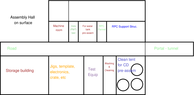
Figure 9.1: Layout of the surface assembly building and storage facilities along the road to the tunnel portal.

The logistics underground also requires special consideration: the storage tanks for Gd-loaded liquid scintillator, pure liquid scintillator and mineral oil will need to be in place prior to the arrival of antineutrino detector elements or completed antineutrino detectors will stack up down in the tunnel waiting to be filled.

9.2 Surface Assembly Building

A surface assembly building of the scale of 25 m$\times$50 m (1250 m²) is required to assemble, survey, and test two antineutrino detectors at once. This building will be large enough to house two detector tanks and their associated inner acrylic vessels. The rest will be stored in the storage building. It will also have a crane of sufficient capacity to assemble the nested vessels and to lift the completed (but dry) antineutrino detectors onto their transporter. The surface assembly building will require clean assembly space for working on the open vessels to maintain the appropriate surface cleanliness. Once the detector modules are assembled and tested as required, they will be moved underground for filling and subsequent installation in the experimental halls.

In parallel with the assembly of the antineutrino detectors, the muon detectors will be inspected and tested. A building of this size will allow us to set up several inspection and testing stations and have a station for survey and alignment. It is sized to handle the assembly of two antineutrino detectors in parallel plus a short incoming RPC panel test station. If the building is arranged in a long (50 m), orientation, a single 30 T bridge crane with rails along the building and a smaller 5–10 T crane utilizing the same rails are sufficient. This allows for the manipulation of partially or fully completed (dry) antineutrino detectors while moving muon detector panels or staging other structures in parallel.

To accomplish these multiple testing, assembly, and QA tasks, appropriate test stations will be assembled. We may need to provide appropriate gas mixes and high and low voltage power as well as a low-noise test environment.

The surface assembly building will be designed to ensure several levels of cleanliness control. Detector components arriving on site will be stored under sealed conditions in the surface assembly building. During the assembly of the detector modules more stringent cleanliness requirements apply. Both the level of particulates and the environmental air will have to be monitored. Cleanrooms of class 1000–10000 inside the surface assembly building or movable clean tents with HEPA filters to cover the detector modules can be used to provide the appropriate environment for the detector assembly.

9.3 Assembly of the Antineutrino Detectors

The major components of the antineutrino detectors will be fabricated at different places worldwide and shipped to the Daya Bay site for assembly and testing. The tasks involved in the assembly of the detector modules include:

1. Cleaning and inspection of stainless steel tank

2. Installation of the PMTs and cabling inside the detector tank

3. Installation of monitoring equipment in tank

4. Lifting the acrylic vessels into the detector tank

5. Connecting all fill lines, calibration, and instrumentation ports

6. Precision survey of tank and acrylic vessel geometry

7. Final cleaning throughout the entire assembly process.

8. Pressure/leak testing of acrylic vessels and detector tank after assembly

9. Test installation of automated calibration systems (to be removed before transport underground)

The entire assembly of the detector modules will be performed in class 1000–10000 cleanroom conditions. This complex assembly and integration task will require close coordination of several working groups (detector design, engineering, calibration, monitoring) and the on-site presence of key scientific and technical personnel.

9.4 Precision Survey of Detector Modules

Before transporting the detector modules underground the geometry of the detector modules is surveyed to high precision using modern laser surveying techniques. The precision commonly achieved in modern equipment over the scale of the antineutrino detector ($\sim 5$ m) is of the order of $<$25 $\mu$m in both the radial and the longitudinal direction. This will serve as a baseline reference for the as-built detector geometry. In-situ monitoring equipment inside the detector modules will then be used to track any changes during the transport or filling of the modules.

Similarly, the muon chambers, PMT support structure and other detector subsystems will be surveyed in the surface assembly building prior to the transport underground. Relating internal system geometries to external fiducial points in the experimental halls will ultimately allow a precise relative understanding of detector geometry to the experimental hall and the outside world.

9.5 Subsystem Testing

Following the assembly of detector modules and subsystems, testing becomes a critical task to ensure a smooth turn on and commissioning the detectors underground. The collaboration’s QA and QC experience, such as from IceCube, will be invaluable in preparing subsystems, getting them ready, and finally installing them underground with a high success rate.

All incoming equipment will be inspected for obvious damage. System elements that are completely assembled and tested to meet specifications at far away sites (the US and Beijing for example) will require a limited retest to ensure no internal damage occurred during shipment. Testing for broken channels or shorts in RPC chambers, PMT function, calibration system function, etc., will all be required. To accomplish these tasks, appropriate test stations will be assembled and utilized in the surface assembly building. The test stations will be manned by technicians, grad students, post-docs and physicists and will utilize a small set of simple electrical tests performed to a written test specification. It is not likely we will repeat all the original performance tests performed at the originating institutions. However, we may need the capability to provide appropriate gas mixes and high and low voltage power as well as a low-noise test environment.

Once the antineutrino detectors have been assembled in the surface assembly building we plan to perform a suite of tests of their mechanical integrity and functionality including

1. pressure and leak tests of the detector tank and acrylic vessels

2. running the PMTs and all cabling with a gas fill inside the detector zones

3. testing the functionality of all ports, calibration, and monitoring equipment

Once a detector module passes these tests it is ready for transport underground. It will be moved down the access tunnel into the underground filling hall on transporters at very low speed.

9.6 Filling the Detector Modules

The underground filling station is designed to accommodate two detector modules during the filling process. The three components: Gd-loaded liquid scintillator, liquid scintillator for the $\gamma$-catcher, and mineral oil will be filled simultaneously into each detector module. The goal is to fill two detector modules from the same batch of liquids to ensure the same target mass and composition in pairs of detectors. They can then be deployed either both at the same near site for a check of the relative detection efficiency, or one at the near and the other one at the far site for a relative measurement of the antineutrino flux. An alternate plan under consideration would be to fill the two detectors in their respective experimental halls. This would require very different logistics and transport arrangements.

The underground filling hall houses a 40-t storage/mixing tank for the 0.1% Gd-liquid scintillator and two more storage tanks for the $\gamma$-catcher scintillator and the mineral oil for the buffer region. All three regions of the detector modules will be filled simultaneously while maintaining equal liquid levels in each vessel to minimize stress and loads on the acrylic vessels. The underground storage tanks are sufficiently large to hold the full liquid volumes for two detector modules.

Dedicated fill lines for the Gd-liquid scintillator, the $\gamma$-catcher liquid scintillator, and the mineral oil connect the storage tank to the detector module during the filling process. The filling station will be equipped with a variety of instrumentation on the storage tanks and the fill lines for a precise and redundant measurement of the target mass and composition. Each fill line may use multiple flowmeters in series for additional systematic control. The instrumentation we envision using during the filling procedure includes (see chapter 6.3):

On the storage tanks

1. liquid level sensors

2. load sensors

3. temperature sensors

4. access ports for extracting liquid samples

In the fill lines

1. Coriolis mass flowmeters + density measurement

2. conventional volume flow meters

3. temperature sensors

In each detector module

1. load sensors in the support of each acrylic vessel

2. liquid level sensors in each zone or volume

3. CCD imaging of inside of detector modules

In addition, all fill lines will be equipped with the necessary filtration and liquid handling systems. The filling of the different detectors will be performed sequentially. This ensures that the same set of instrumentation and flowmeters is used in determining the target mass in each detector. In this scenario the systematic uncertainty on the relative target mass between detector modules comes from the repeatability of the mass flow measurements of one set of instrumentation while the uncertainty on the relative masses between different detector zones (which is less critical) comes from the absolute difference between different sets of instrumentation. After filling, the two detector modules will be deployed in the appropriate experimental halls.

9.7 Transport to Experimental Halls

Detector modules and related systems will be transported to the filling hall and experimental halls from the surface assembly building using flat-bed trailers or self-propelled transporters. There are several issues associated with this task that make it somewhat more difficult than simply using conventional transportation equipment:

1. Due to cost and civil construction constraints the tunnel itself is not very large.

2. Entrance to the underground laboratory is through an access tunnel with an incline of up to 10%.

3. Transport systems have to be compliant with ventilation and underground safety requirements.

Because of this, the transport mechanism should:

1. have a low bed height ($\leq$0.5 m).

2. be powered by an electric drive or by some very clean burning fuel such as propane gas.

3. be capable of accurate tracking along an electric or mechanical guide.

4. utilize an active horizontal level mechanism while transporting the antineutrino detector down the 10% entrance tunnel into underground laboratory. This will maintain the detector in an upright and vertical position and minimize any stress on the inner acrylic vessels.

Note that the detector modules will be filled in the underground filling station and they will only be transported in the horizontal tunnels between experimental halls after they have been filled. During the transport to the experimental halls the antineutrino detectors are filled and have a total mass of $\sim$100 T. We are currently investigating several transportation systems. Custom-made (short and wide) flatbed, ‘lowboy’ trailers pulled by an electric airport pushback tugs are one option. A second option is self-propelled, remote-controlled, small wheel diameter transporters which often have hydraulic lifting capability. A third option is an electric power train-like transporter which runs on rails. All of these systems have the benefit of having a bed height of around 0.5 m. All of these can be powered by electric motors for clean, safe operation in confined spaces.

9.8 Final Integration in the Experimental Halls

After the antineutrino detectors have been filled they will be slowly transported through the tunnels to the appropriate experimental halls. They will be deployed by crane into the drained water pool and onto their stands. All cabling and electronics will be connected and their calibration systems installed so they can be calibrated and checked.

The muon-detector elements (RPC chambers, structures and PMTs) will be delivered to the experimental halls after test and checkout on the surface. These elements will be installed in the pool (PMTs and PMT supports) and over the roof of the pool (RPCs).

9.9 Early Occupancy of the Experimental Halls at the Near and Mid Sites

The civil construction of the underground laboratory including the experimental halls and tunnels will take about 24 months. The time scale is set by the excavation of the tunnels between the experimental halls. The near and mid sites will be completed first before the tunnel to the far site is finished. Completion of experimental halls at the Daya Bay near site and the mid site suggests the implementation of an early experiment utilizing the halls at these two sites. Early occupancy of these sites would provide the opportunity to commission the detector modules at the near site and to make a first, “fast” measurement with a sensitivity of sin${}^{2}2\theta_{13}<$0.035 (see Chapter 3).

The use of these experimental halls during the ongoing excavation and construction of the tunnel to the far site poses significant but not insurmountable logistical challenges for the work underground. While shared underground occupancy is largely to be avoided because of issues of safety (traffic, blasting, explosives, fumes etc..) and interference with mining work other experimental facilities such as KamLAND in the Kamioka mine have demonstrated that data taking with a sensitive neutrino experiment is possible while a new underground hall is excavated some few hundred feet away. In the case of KamLAND, a new underground hall for a liquid scintillator purification system was built in 2006. The experiment continued data taking and access to the experimental facilities for scientists was arranged on a specific schedule together with the mining and construction crews. A similar situation can be found at SNOLab in the Creighton mine in Canada which is being constructed during the active phase of the Sudbury Neutrino Observatory.

The possibility of commissioning the detector modules at the near site and making an early measurement of sin${}^{2}2\theta_{13}$ with detector modules at the near and mid sites may be worth the additional logistical challenge of coordinating the underground construction work and the installation of the first detector modules. In this case, the experiment may start commissioning detector modules 18 months after beginning of civil construction and taking first neutrino data at two different experimental halls and distances about two years after breaking ground.

The planning for this scenario requires that

1. the necessary infrastructure for the operation of the detector modules (power, air, etc) can be installed at the near and mid sites while the construction of the tunnel to the far site is ongoing.

2. a plan for the installation of the detector modules will be developed that does not impact the day-to-day mining operation

3. safety issues with respect to escape routes and personnel underground are addressed

This possibility requires further discussion and negotiations with the contractors for the underground construction of the tunnel and experimental halls.

9.10 Precision Placement and Alignment

Precise knowledge of the ‘global’ location of each hall with respect to the reactor cores is important for the accurate determination of the distances between the reactor cores and each neutrino detector. Permanent survey markers in each experiment hall will serve as reference marks for the positioning of the detectors. These survey markers will be placed and known to a precision of better than tens of centimeters, with respect to the outside world, even though the halls are hundreds of meters inside underground tunnels. This precision is commonly achieved in the construction of tunnels and in mining.

Within the experimental halls the position of the detectors can be determined quite precisely. The antineutrino detectors will be surveyed into approximate but precisely known location on their stands at the bottom of each water pool. The knowledge of the location of each antineutrino detector, with respect to the fiducial markers in the halls, will be at the sub-mm level. The location of the muon system elements also can be surveyed and understood at the same sub-mm level. This is both with respect to the antineutrino detectors and the experimental hall.

With this information the distance between the detector modules and the reactor cores will be known to the required precision of better than 30 cm.

Element of Experiment	Positioning Accuracy
experimental hall	$\mathcal{O}$(10 cm)
detector position in experimental hall	$<$ mm
acrylic vessels within detector tank	$<25$ $\mu$m

Table 9.1: Positioning accuracy of the principal elements of the Daya Bay experiment.

10 Operations of the Daya Bay Experiment

Operation of the Daya Bay Experiment requires a variety of tasks including:

1. Underground transport of detector modules and deployment into the experimental halls.

2. Data taking with the detector modules in the experimental halls.

3. Frequent automated calibration of each detector module.

4. Full-volume calibration of the detector modules as needed.

5. Monitoring of the state of the detector modules and the underground lab conditions.

6. Monitoring and maintenance of the muon system.

7. Maintenance and repair of the calibration system.

8. Monitoring, maintenance, and repair of electronics and data acquisition system.

9. Monitoring the target liquid and and performing regular chemical assays on the liquid scintillator samples.

The routine monitoring of the experiment will be performed by members of the collaboration and special technical personnel trained in emergency procedures of the underground lab facility. A surface control room will be set up in the vicinity of the access portal for monitoring and data taking. Daily walk-around checks in the underground facility will ensure the safe operation of all underground systems.

The operations of the detector will consist of monitoring the detector performance and data quality, routine calibration, and online data analysis. The calibration procedure will include automated calibration runs to be performed by shift members operating the detector. Special manual calibration runs are to be performed by expert personnel.

All shift duties related to data taking and monitoring will be shared between the members of the Day Bay Collaboration. On-site shifts as well as remote, off-site shifts will be part of running the Daya Bay experiment. Groups responsible for specific subsystems will make arrangements for the maintenance of detector subsystems.

The scientific and technical team of the Daya Bay experiment will have support from the China Guangdong Nuclear Power Group (CGNPG) which operates the Daya Bay reactor complex, and which is a collaborator on the experiment.

Operation of the Daya Bay experiment includes data taking with the detector modules in different configurations. The default configuration, as well as other optional configurations, are outlined in the following section. A variety of alternative operations plans are currently being evaluated with varying frequency of detector swaps.

10.1 Configurations of Detector Modules

This section describes the different possible detector configurations of the Day Bay experiment and their possible use during different phases of the experiment. The different deployment options and run scenarios are currently being evaluated from the point of view of logistics, cost and physics reach:

1. Initial Detector Deployment: The eight detector modules are built, assembled, and filled in pairs to ensure that their characteristics and target mass and composition are as identical as possible. Once a detector pair has been filled underground there are two options:

   1. the detectors can either be deployed together at the Daya Bay near site for a commissioning run and check of their relative detector efficiencies, or

   2. one of them can be installed at the near site and the other one at the mid or far site to immediately start data taking with two detectors of the same pair at different distances

   A commissioning run of both detectors at the near hall is a unique opportunity to test the operation of each detector module before one of them is deployed at the mid or far site. The intrinsic detector background, the cosmogenic background at the near site, and the relative detection efficiency of the detector modules can be checked during this commissioning phase. This step is trivial for the first detector pair, as the default plan for the Daya Bay near site allows for the installation of two detector modules. Commissioning of the other detector pairs at the near site requires deploying the detectors to the other experimental halls immediately after the commissioning run. A drawing of the detector configuration is shown in Fig. 10.1.

   

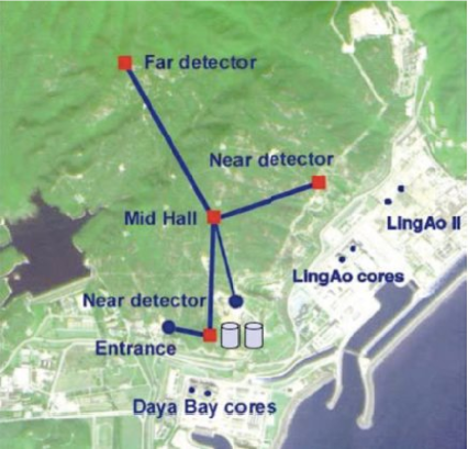
   Figure 10.1: Optional commissioning runs of pairs of detectors at the Daya Bay near site. With sufficient runtime of a few months for systematic checks of the detectors a relative comparison of the detector response is possible.

   Including the time for detector installation and start-up, the total time for such a commissioning run is likely to be $\sim$6 months. The collaboration may decide to skip this initial commissioning step and immediately deploy the two detectors from each pair at the near and far (or mid) sites to expedite the overall experiment. In this second scenario two detectors are assembled and filled at the same time and then one of them is deployed at a near site and the other one is immediately moved to the far site. Data taking and a relative measurement of the neutrino flux between these two detectors can then commence immediately.

2. Using the Mid Site: The default plan for the construction of the underground laboratory at Daya Bay includes a mid-site at a distance of about 1156 m from the Daya Bay cores and 873 m from the center of the Ling-Ao cores (as discussed in Section 2.1). Civil construction of this site will finish earlier than the excavation of the tunnel to the far site. By deploying two or four 20-ton detector modules at the mid-site along with two 20-ton detectors at the Daya Bay near it may be possible to make a first, “fast” measurement of sin${}^{2}2\theta_{13}$ at this intermediate distance. See chapter 9 for a discussion of the logistical and construction issues relating to early occupancy of the near and mid sites. A drawing of this detector configuration is shown in Fig. 10.2.

   

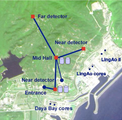
   Figure 10.2: Optional near-mid configuration of the Daya Bay experiment for an early physics run. With two 20-ton detectors at the near and mid site a sensitivity of sin${}^{2}2\theta_{13}\sim$0.035 can be achieved in $\sim$1 year of data taking.

   One can also envision using the mid-site for a systematic cross check. By running the experiment in the mid-far configuration it is possible to probe the $\theta_{13}$ oscillation with a different combination of distances. The ultimate sensitivity of the experiment is somewhat reduced but the ratio of the energy spectra from the mid and far site provide a different oscillation signature as a function of energy.

3. Default Configuration of Full Experiment: To achieve the best sensitivity in the Daya Bay experiment two 20-ton detector modules are deployed at each one of the Daya Bay and Ling-Ao near sites along with four 20-ton detector modules at the far site. The total active target mass at the far site is 80 tons. In the default scenario, the mid-site is unused. It is possible to operate in this configuration either with or without the swapping of pairs of detectors. A drawing of this detector configuration is shown in Fig. 10.3.

   

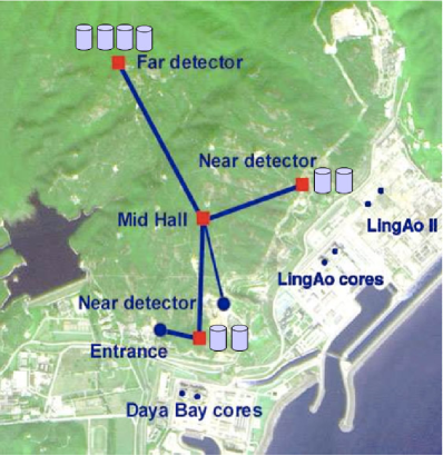
   Figure 10.3: Default configuration of the Daya Bay experiment, optimized for best sensitivity in sin${}^{2}2\theta_{13}$. Data taking can occur in a static configuration or with swapping of detectors.

4. Optional Swapping in the Daya Bay Run Plan: Swapping of detector modules is an option but not a necessity in the Daya Bay experiment. The target sensitivity of sin${}^{2}2\theta_{13}<0.01$ at 90% C.L. can be achieved without swapping detectors. The design of the Daya Bay experiment provides the option of swapping detectors for systematic checks and to ultimately increase the sensitivity of the experiment to about sin${}^{2}2\theta_{13}<0.006$ (see Table 3.9). After all detectors are commissioned and located at their initial sites swapping of detectors can occur either:

   1. throughout the experiment in regular 6-months intervals for the optimal cancellation of the experimental systematics (as described in Table 3.3), or

   2. after an initial static experiment with data taking for 2-3 years that reaches the design goal of sin${}^{2}2\theta_{13}<0.01$

   The collaboration has not decided yet which approach to choose. It will depend on the outcome of the design studies of the antineutrino detectors, their transportation system, and R&D on the calibration and monitoring of the detector response. In addition, the timeliness and potential impact of a first measurement of $\theta_{13}$ at Daya Bay will drive the detector deployment and run plan.

10.2 Detector Swapping

The purpose of swapping detectors has been described in Sections 2 and 3. An overview of the steps involved in the swapping procedure is given below. Detector swapping will utilize the standard transportation methods developed for the underground movement of the detectors. As such, detector swapping uses all of the same techniques and procedures that are developed for the initial deployment of the detector modules and the installation of the experiment. Even the initial deployment of the detector modules at the far site requires filled modules to be transported from the filling station to the far experimental hall. Swapping is different from the initial deployment of the detector modules in that it is critical to characterize any change in the detector response during the swap. Without a complete characterization of the detector response the performance of a module cannot be compared before and after the swap. This poses a unique challenge and sets the criteria for the development of a comprehensive calibration and monitoring program.

10.3 Logistics of Detector Swapping

The total estimated time for detector swapping in the baseline water pool configuration is several days. We anticipate that the transport of each detector module in the tunnel can be performed in less than a day. With a transportation speed of $\sim$5 m/minute a distance of 1500 m can be covered in less than 7 hrs.

Detector swapping includes the following sequence of steps:

1. Perform final detector calibration to establish detector response immediately prior to the move.

2. Shut down HV and DAQ.

3. Disconnect large area RPC roof system as necessary to ready this portion of muon system for sliding back and out of the way for antineutrino detector lift operation.

4. Drain water pool to a level below the antineutrino detector module ($\sim$1000–1500 m³). (Replace with fresh, filtered water when refilling.)

5. Install a personnel man bridge over the open pit to allow safe access to the top of antineutrino detector.

6. Disconnect PMT HV and signal cables, LS overflow plumbing, etc. as required to prepare for move.

7. Remove calibration system & piping as required from top of antineutrino detector.

8. Attach the lifting device to the antineutrino detector.

9. Using a 150 T crane, lift the antineutrino detector vertically out of pool and translate it horizontally onto a transporter.

10. Transport the antineutrino detector to the new location.

11. Reverse the operation at the previously prepared new location.

12. Calibrate the detector in the new location to establish the detector response immediately after the move.

11 Schedule and Scope

In this chapter, the overall project plan will be described. This will include an overview of the project schedule, and the concept for the international division of scope. Later, the planned U.S. scope range will be outlined. This is a joint project with an international collaboration.

11.1 Project Schedule

Briefly, the first significant construction event of the Daya Bay experiment schedule begins with the initiation of civil construction on the tunnels in the spring of 2007. The Project’s goal is to complete the civil construction of the tunnels, experimental halls and utility infrastructure before the middle of 2009.

There is an additional goal to complete the Daya Bay Near Hall (and Filling Hall) as early as possible — approximately 12 months earlier than the final (far) hall. The schedule for the detector elements is therefore driven by the completion of the first two antineutrino detectors and one third of the muon system hardware by the fall of 2008 in order to deploy these in this first experimental hall. This Daya Bay Near Hall will be used as an early opportunity to install, test and begin partial experiment operations — a chance to debug and gain insight into detector operations. This would occur in the early summer of 2009. The next hall to follow will be the Mid Hall. This hall and its detectors will most likely be available for installation tasks 3–4 months after the Daya Bay Near Hall (early in calendar 2009). This would then allow us an opportunity to install and begin measurements of $\theta_{13}$ by late summer of 2009.

The remainder of the detectors will be installed and commissioned in the Ling Ao Near and Far Halls by early summer of calendar 2010 so that the full complement of near and far detectors can begin data taking. A more complete view of the project schedule is shown in Fig. 11.1 below.

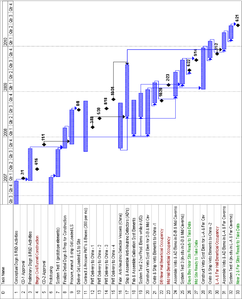
Figure 11.1: Daya Bay Project Summary Schedule.

11.2 Project Scope

The project’s entire technical scope has been described in the previous chapters. The total Daya Bay project includes the civil construction of the experimental facility at the Daya Bay nuclear reactor complex as well as the construction of the detector elements (antineutrino detectors, muon system, calibration system, DAQ/Trigger/Online and offline). Crucial to all of these activities are the project integration elements: Installation and System Test, System Integration and Project Management.

The division of the Project scope will not be finalized until a formal MOU is developed and signed between the U.S., China and other countries. Therefore, the scope shown in Table 11.1 is based on the current status of discussions within the Collaboration.

WBS	Description	China	U.S.
		lead	lead
1	Antineutrino Detector	X
	System design, steel vessels, LS, mineral oil	*
	FEE co-design and manufacture, racks	*
	safety systems, assem. and test	*
	Gd-LS, LS purification/mixing/filling	$\circ$	$\circ$
	acrylic vessels, PMTs and support,		*
	transporter, FEE co-design, cables, crates		*
2	Muon System		X
	System design, muon tracker, water Cherenkov		*
	PMTs and support, assem. and test		*
	FEE, safety systems	*
3	Calibration and Monitoring		X
	automated system, glove box		*
	monitoring system and system test		*
	manual system, LED, radioactive sources	*
	low background counting system	*
4	Trigger/DAQ/Online	X
	Trig/DAQ board co-design and manufacture	*
	monitoring/controls hardware and software	*
	racks	*
	Online hardware and software	$\circ$	$\circ$
	Trig/DAQ board co-design, crates, cables		*
	system test platform		*
5	Offline	$\circ$	$\circ$
	offline architecture and data archiving in U.S.		*
	offline hardware and software and simulations	$\circ$	$\circ$
6	Conventional Construction	X
	tunnels, halls, underground utilities	*
	safety systems, surface facilities	*
7	Installation and Test	$\circ$	$\circ$
	Onsite installation and system testing	$\circ$	$\circ$
	planning, execution	$\circ$	$\circ$
8	System Integration	$\circ$	$\circ$
	System level mechanical engineering	$\circ$	$\circ$
	System level electronics engineering	$\circ$	$\circ$
	Common Fund
9	Project Management	$\circ$	$\circ$
	Planning, communication, coordination	$\circ$	$\circ$
	reporting, reviews	$\circ$	$\circ$

Table 11.1: Daya Bay project scope. The X’s refer to which country has the lead on a given task. The *’s refer to responsibility for scope deliverables. The $\circ$’s refer to shared responsibility.

The major elements of U.S. scope deliverables include parts of the antineutrino detector: Gadolinium loaded Liquid Scintillator, PMTs (w/bases and control boards), PMT support structure and the transporter system for moving the assembled and filled antineutrino detectors. The U.S. scope also includes the majority of the Muon System: the PMT based water Cherenkov system and the roof tracking system (possibly RPCs). A significant portion of the Calibration system will also be a U.S. deliverable: the automated deployment system and the full monitoring system. Additionally, many elements will be cooperatively developed: the front-end and trigger electronics design for both the antineutrino and muon systems and many of the infrastructure items (e.g., online and offline software). System design integration, installation and test and project management will be jointly planned, managed and executed by the U.S. and China.

Appendix A Acknowledgements

This work was supported in part by the the Chinese Academy of Sciences, the National Natural Science Foundation of China (Project numbers 10225524, 10475086, 10535050 and 10575056), the Ministry of Science and Technology of China, the Guangdong provincial goverment, the Shenzhen Municipal government, the China Guangdong Nuclear Power Group, the Research Grants Council of the Hong Kong Special Administrative Region of China (Project numbers 400805 and 400606), the United States Department of Energy (Contracts DE-AC02-98CH10886, DE-AS02-98CH1-886, and DE-FG02-91ER40671 and Grant DE-FG02-88ER40397), the U.S. National Science Foundation (Grants PHY-0555674 and NSF03-54951), the University of Houston (GEAR Grant number 38991), the University of Wisconsin and the Ministry of Education, Youth and Sports of the Czech Republic (Project numbers MSM0021620859 and LC527).

Appendix B Acronyms

AC	alternating current
Access	database program from Microsoft Corporation
ADC	analog to digital converter
BES	Beijing Spectrometer at the Beijing Electron Positron Collider
BINE	Beijing Institute of Nuclear Energy
BNL	Brookhaven National Laboratory
CAS	Chinese Academy of Sciences
CC	charged-current neutrino interactions
CCG	central clock generator
CD-1	Critical Decision #1 — Site Selection (CDR)
CD-2	Critical Decision #2 — Cost/Schedule/Scope well defined (TDR)
CERN	European Organization for Nuclear Research
CGNPC	China Guandong Nuclear Power Group (Daya Bay owner)
CL	confidence level
$CP$	charge, parity symmetry
$CPT$	charge, parity, time reversal symmetry
CVS	code versioning system
DAC	digital to analog converter
DAQ	data acquisition
DC	direct current
DCS	detector control system
DOE	U.S. Department of Energy
ES	elastic neutrino scattering
ES&H	environment, safety & health
FADC	flash ADC
FEC	front-end card
FEE	front-end electronics
FET	field effect transistor
FPGA	field programmable gate array
FY	fiscal year
FWHM	full width at half maximum
Gallex	Gallium Experiment
Gd-LS	Gd loaded liquid scintillator
GEANT	detector description and simulation tool
GNO	Gallium Neutrino Observatory
GOC	global operation clock
GPS	Global Positioning System
H/C	ratio of hydrogen to carbon
H/Gd	ratio of hydrogen to gadolinium
HOTLink	bus for clock distribution
HV	high voltage
HVPS	high voltage power supplies

IFC	International Finance Committee
IGG	Institute of Geology and Geophysics
IHEP	Institute for High Energy Physics
ILL	Institut Laue-Langevin
ISO	International Standards Organization
JINR	Joint Institutes for Nuclear Research
JTAG	electronic standard for testing & downloading FPGA’s
KamLAND	Kamioka Liquid Scintillator Antineutrino Detector
K2K	KEK to Kamiokanda neutrino oscillation experiment
KARMEN	Karlsruhe Rutherford Medium Energy Neutrino experiment
KEK	High Energy Accelerator Research Organization in Japan
Kr2Det	Two Detector Reactor Neutrino Oscillation experiment at Krasnoyarsk
$L/E$	distance divided by energy
L3C	L3 cosmic ray experiment
LAB	Linear Alkyl Benzene
LabVIEW	Laboratory Virtual Instrument Engineering Workbench
LBNL	Lawrence Berkeley National Laboratory
LED	light emitting diode
LENS	Low Energy Solar Neutrino Spectrometer
LIGO	Laser Interferometric Gravity Observatory
LMA	Large Mixing Angle solution
Ln	lanthanides
LS	liquid scintillator
LSND	Liquid Scintillator Neutrino Detector
LVDS	low voltage differential
MBLT	Multiplexed Block Transfer
m.w.e.	meters of water equivalent
MC	Monte Carlo
MINOS	Main Injector Neutrino Oscillation experiment
MoST	Ministry of Science and Technology of China
MOU	Memorandum of Understanding
MSB	1,4-bis[2-methylstyrl]benzene
MSPS	mega-sample per second
NC	neutral current neutrino interactions
NSFC	Natural Science Foundation of China
NPP	nuclear power plant
NTP	Network Time Protocol
ODH	oxygen deficiency hazard
OPERA	Oscillation Project with Emulsion-tRacking Apparatus
p.e.	photo-electrons
PC	pseudocumene
PC	personal computer
PMT	photomultiplier tube
PPS	Pulse Per Second
PRD	Pearl River Delta (elevation above sea level)
PVC	Poly Vinyl Chloride
PWR	pressurized water reactors

QA	quality assurance
QC	Quality control
QE	quantum efficiency
REE	rare earth elements
R&D	research and development
RS	Richter scale
RPC	resistive plate chamber
RPVC	rigid polyvinyl chloride
SAGE	Soviet American Gallium solar neutrino Experiment
SCADA	supervisory, control, and data acquisition
s.p.e.	single photo-electron
SNO	Sudbury Neutrino Observatory
SNO+	proposed solar and geo-neutrino experiment using liquid scintillator in the existing SNO detector
SS	stainless steel
SAB	surface assembly building
TDC	time to digital converter
TSY	Fourth Survey and Design Institute of China Railways
UTC	Universal Coordinated Time
UV	ultraviolet light
VME	Versa Module Europa
WBS	work-breakdown structure
YREC	Yellow River Engineering Consulting Co. Ltd.

References

- [1] For a recent review, see V. Barger, D. Marfatia, and K. Whisnant, Int. J. Mod. Phys. E 12 (2003) 569 [arXiv:hep-ph/0308123].
- [2] Q.R. Ahmad et at. (SNO Collaboration), Phys. Rev. Lett 87 071301 [arXiv:nucl-ex/0106015]; 89 (2002) 011301 [arXiv:nucl-ex/0204008]; 89 (2002) 011302 [arXiv:nucl-ex/0204009]; 92 (2004) 181301 [arXiv:nucl-ex/0309004]; Phys. Rev. C72 (2005) 055502 [arXiv:nucl-ex/0502021].
- [3] Y. Fukuda et al. (SuperK Collaboration), Phys. Rev. Lett., 81 (1998) 1158 [arXiv:hep-ex/9805021]; 82 (1999) 2430 [arXiv:hep-ex/9812011]; S. Fukuda et al., Phys. Rev. Lett. 86 (2001) 5651 [arXiv:hep-ex/010302]; M. B. Smy et al., Phys. Rev. D69 (2004) 011104 [arXiv:hep-ex/0309011].
- [4] B. T. Cleveland et al., Astrophys. J. 496 (1998) 505.
- [5] J. N. Abdurashitov et al. (SAGE Collaboration), J. Exp. Theor. Phys. 95 (2002) 181 [arXiv:astro-ph/0204245]; W. Hampel et al. (GALLEX Collaboration), Phys. Lett. B447 (1999) 127; M. Altman et al. (GNO Collaboration), Phys. Lett. B490 (2000) 16 [arXiv:hep-ex/0006034].
- [6] K. Eguchi et al. (KamLAND Collaboration), Phys. Rev. Lett., 90 (2003) 021802 [arXiv:hep-ex/0212021]; 94 (2005) 081801 [arXiv:hep-ex/0406035].
- [7] Y. Fukuda et al. (SuperK Collaboration), Phys. Lett. B433 (1998) 9 [arXiv:hep-ex/9803006]; B436 (1998) 33 [arXiv:hep-ex/9805006]; Phys. Rev. Lett., 81 (1998) 1562 [arXiv:hep-ex/9807003]; S. Fukuda et al., Phys. Rev. Lett. 85 (2000) 3999 [arXiv:hep-ex/0009001]; Y. Ashie et al., Phys. Rev. Lett. 93 (2004) 101801 [arXiv:hep-ex/0404034].
- [8] E. Aliu et al. (K2K Collaboration), Phys. Rev. Lett. 94 (2005) 081802 [arXiv:hep-ex/0411038].
- [9] D.G. Michael et at. (MINOS Collaboration), Observation of muon neutrino disappearance in the MINOS detectors with the NuMI neutrino beam [arXiv:hep-ex/0607088].
- [10] M. Apollonio et al. (Chooz Collaboration), Eur. Phys. J. C27, 331 (2003) [arXiv:hep-ex/0301017].
- [11] F. Boehm et al. (Palo Verde Collaboration), Phys. Rev. D62, 072002 (2000) [arXiv:hep-ex/0003022].
- [12] C. Athanassopoulos et al. (LSND Collaboration), Phys. Rev. C54 (1996) 2685 [arXiv:hep-ex/9605001]; Phys. Rev. Lett. 77 (1996) 3082 [arXiv:hep-ex/9605003]; A. Aguilar et al., Phys. Rev. D64 (2001) 112007 [arXiv:hep-ex/0204049].
- [13] K. Eitel et al. (KARMEN Collaboration), Nucl. Phys. Proc. Suppl. 91 (2000) 191 [arXiv:hep-ex/0008002]; B. Armbruster et al., Phys. Rev. D66 (2002) 112001 [arXiv:hep-ex/0203021].
- [14] S. Doldelson, A. Melchiorri, and A. Slosar, Phys. Rev. Lett. 97 (2006) 04301 [arXiv:astro-ph/0511500].
- [15] I. Stancu et al., The MiniBooNE detector technical design report, FERMILAB-TM-2207, May 2001.
- [16] Z. Maki, M. Nakagawa, and S. Sakata, Prog. Theor. Phys. 28 (1962) 870; B. Pontecorvo, Sov. Phys. JETP 26 (1968) 984; V.N. Gribov and B. Pontecorvo, Phys. Lett. B28 (1969) 493.
- [17] R.N. Mohapatra et al., Theory of Neutrinos: A white paper [arXiv:hep-ph/0510213].
- [18] G.L. Fogli, E. Lisi, A. Marrone, and A. Palazzo, and A.M. Rotunno, 40th Rencontres de Moriond on Electroweak Interactions and Unified Theories, La Thuile, Aosta Valley, Italy, 5-12 March 2005 [arXiv:hep-ph/0506307].
- [19] T. Schwetz, Talk given at 2nd Scandinavian Neutrino Workshop (SNOW 2006, Stockholm Sweden, 2-6 May 2006 [arXiv:hep-ph/0606060].
- [20] ‘Recommendations to the Department of Energy and the National Science Foundation on a U.S. Program of Reactor- and Accelerator-based Neutrino Oscillations Experiments’, http://www.science.doe.gov/hep/NuSAG2ndRptFeb2006.pdf
- [21] The Neutrino Matrix, http://www.aps.org/neutrino/
- [22] K. Anderson, et al., White paper report on using nuclear reactors to search for a value of [arXiv:hep-ex/0402041].
- [23] R.N. Mohapatra, Talk at the 11th International Workshop on Neutrino Telescopes, Venice, Italy, 22-25 Feb. 2005 [arXiv:hep-ph/0504138].
- [24] V. Barger, D. Marfatia and K. Whisnant, Phys. Rev. D65 (2002) 073023 [arXiv:hep-ph/0112119].
- [25] V. Barger, D. Marfatia and K. Whisnant, Phys. Lett. B560 (2003) 75 [arXiv:hep-ph/0210428]; P. Huber, M. Lindner and W. Winter, Nucl. Phys. B654 (2003) 3 [arXiv:hep-ph/0211300]; H. Minakata, H. Nunokawa and S. Parke, Phys. Rev. D68 (2003) 013010 [arXiv:hep-ph/0301210].
- [26] V. D. Barger, D. Marfatia and K. Whisnant, “Neutrino Superbeam Scenarios At The Peak,” in Proc. of the APS/DPF/DPB Summer Study on the Future of Particle Physics (Snowmass 2001) ed. N. Graf, eConf C010630 (2001) E102 [arXiv:hep-ph/0108090].
- [27] H. Minakata et al., Phys. Rev. D68 (2003) 033017 [Erratum-ibid. D70 (2004) 059901] [arXiv:hep-ph/0211111]; P. Huber, M. Lindner, M. Rolinec, T. Schwetz and W. Winter, Phys. Rev. D70 (2004) 073014 [arXiv:hep-ph/0403068]; K. Hiraide et al., Phys. Rev. D73 (2006) 093008 [arXiv:hep-ph/0601258].
- [28] C.L. Cowan, F. Reines, F.B. Harrison, H.W. Kruse, and A.D. McGuire, Science 124 (1956) 103.
- [29] M.F. James, J. Nucl. Energy 23 517 (1969).
- [30] L. Miller, Ph.D Thesis, Stanford University, 2000, unpublished.
- [31] V.I. Kopeikin, Phys. Atom. Nucl. 66 (2003) 472 [arXiv:hep-ph/0110030].
- [32] B. Achkar et al., Phys. Lett. B374 243 (1996).
- [33] K. Schreckenbach et al., Phys. Lett. B160, 325 (1985); A. A. Hahn et al., Phys. Lett. B218, 365 (1989).
- [34] P. Vogel and J. Engel, Phys. Rev. D39, 3378 (1989).
- [35] P. Vogel and J. F. Beacom, Phys. Rev. D60, 053003 (1999) [arXiv:hep-ph/9903554].
- [36] K. S. Hirata et al., Phys. Lett. B205, 416 (1988); Y. Fukuda et al., Phys. Lett. B335, 237 (1994).
- [37] L.A. Mikaelyan and V.V. Sinev, Phys.Atomic Nucl. 63 1002 (2000) [arXiv:hep-ex/9908047].

References

- [1] L. A. Mikaelyan and V. V. Sinev, Phys. Atom. Nucl. 63, 1002 (2000); L. Mikaelyan, Nucl. Phys. Proc. Suppl. 91, 120 (2001); L. A. Mikaelyan, Phys. Atom. Nucl. 65, 1173 (2002).
- [2] Report of Preliminary Feasibility Study of Site Selection for the Daya Bay Neutrino Experiment, prepared by Beijing Institute of Nuclear Energy, September, 2004.
- [3] Y.F. Wang, Nucl. Instr. and Meth. A503, 141 (2003); M.J. Chen et al., Nucl. Instr. and Meth.A562, 214 (2006).
- [4] M. Apollonio et al. (Chooz Collaboration), Phys. Lett. B420, 397 (1998); Phys. Lett. B466, 415 (1999); Eur. Phys. J. C27, 331 (2003).
- [5] F. Boehm et al. (Palo Verde Collaboration), Phys. Rev. Lett. 84, 3764 (2000) [arXiv:hep-ex/9912050]; Phys. Rev. D62, 072002 (2000) [arXiv:hep-ex/0003022]; Phys. Rev. D64, 112001 (2001) [arXiv:hep-ex/0107009]; A. Piepke et al., Nucl. Instr. and Meth. A432, 392 (1999).
- [6] J.W. Zhang et al., High Energy Phys. and Nucl. Phys., 27, 615 (2003); JiaWen Zhang et al., Nucl. Instrum. Meth. A540, 102 (2005).

References

- [1] M. Apollonio et al., Phys. Lett. B420, 397 (1998); Phys. Lett. B466, 415 (1999); Euro. Phys. J. C27, 331 (2003).
- [2] L. A. Mikaelyan and V. V. Sinev, Phys. Atom. Nucl. 63, 1002 (2000); L. Mikaelyan, Nucl. Phys. Proc. Suppl. 91, 120 (2001); L. A. Mikaelyan, Phys. Atom. Nucl. 65, 1173 (2002).
- [3] V. Kopeikin, L. Mikaelyan, V. Sinev, Phys. Atom. Nucl. 64, 849 (2001); V. Kopeikin, L. Mikaelyan, V. Sinev [arXiv:hep-ph/0412044].
- [4] K. Eguchi et al., Phys. Rev. Lett. 90, 021802 (2003).
- [5] T. Gaisser, Cosmic Rays and Particle Physics, Cambridge University Press, 1991.
- [6] D. Chirkin, [arXiv:hep-ph/0407078].
- [7] J. Kremer et al., Phys. Rev. Lett. 83, 4241 (1999)
- [8] H. Jokisch et al., Phys. Rev. D19, 1368 (1979).
- [9] P. Antonioli et al., Astro. Phys. 7, 357 (1997).
- [10] Y. F. Wang et al., Phys. Rev. D64, 013012 (2001).
- [11] T. Hagner et al., Astro. Phys. 14, 33 (2000).
- [12] J. Boger et al., Nucl. Instr. and Meth. A449, 172 (2000).
- [13] M.G.T. Lasserre, [arXiv:hep-ex/0606025].
- [14] T. Araki et al., (KamLAND Collaboration) Phys. Rev. Lett. 94, 081801 (2005).
- [15] Liangjian Wen et al., Nucl. Instr. and Meth. A564, 471 (2006).
- [16] P. Huber, M Lindner, T. Schwetz, and W. Winter, Nucl. Phys. B665, 487 (2003); Nucl. Phys. B645, 3 (2002).
- [17] D. Stump et al., Phys. Rev. D65, 014012 (2001).
- [18] Y. Fukuda et al., Phys. Rev. Lett. 81, 1562 (1998); Y. Ashie et al., [arXiv:hep-ex/0501064].
- [19] H. Minakata, H. Sugiyama, O. Yasuda, K. Inoue, and F. Suekane, Phys. Rev. D68, 033017 (2003); H. Minakata and H. Sugiyama, Phys. Lett. B580, 216 (2004).
- [20] Y. Declais et al., Phys. Lett.B338, 383 (1994); B. Ackar et al., Nucl. Phys. B434, 503 (1995); B. Ackar et al., Phys. Lett. B374, 243 (1996).
- [21] H. Sugiyama and O. Yasuda, [arXiv:hep-ph/0508090].

References

- [1] Report of Preliminary Feasibility Study of Site Selection for the Daya Bay Neutrino Experiment, prepared by Beijing Institute of Nuclear Energy, September, 2004.
- [2] Catalog of Chinese Earthquakes, Quoted in the Preliminary Safety Report on Ling Ao Nuclear Power Plant.
- [3] Report of Ling Ao Nuclear Power Plant.
- [4] Report on Geo-technical Survey(Feasibility Study and Conceptual Design), Institute of Geology and Geophysics, CAS, May, 2006.
- [5] Final Report on Topographic Survey of the Neutrino Experimental Site, Institute of Geology and Geophysics, CAS, June, 2006.
- [6] Map obtained from Topographic Survey of the Neutrino Experimental Site, Institute of Geology and Geophysics, CAS, December, 2005.
- [7] Report on Engineering Geology of the Neutrino Experimental Site, Institute of Geology and Geophysics, CAS, May 6, 2006.
- [8] Report on Geophysical Survey of the Neutrino Experimental Site, Institute of Geology and Geophysics, CAS, May 6, 2006.
- [9] Report on Bore Drilling and In-situ Sonic Investigation of the Neutrino Experimental Site, Institute of Geology and Geophysics, CAS, May, 2006.
- [10] Report on Stress-loading in Bore Holes at the neutrino Experimental Site, Institute of Geology and Geophysics, CAS, April 18, 2006.
- [11] Report on Ultra-sonic Imaging in Bore holes at the Neutrino Experimental Site, Institute of Geology and Geophysics, CAS, May, 2006.
- [12] Report on Laboratory Study of the Neutrino Experimental Site, Institute of Geology and Geophysics, CAS, May 6, 2006.
- [13] Feasibility study about Daya Bay neutrino experiment engineering work, The Fourth Survey and Design Inst. of China Railway, July 2006.
- [14] Feasibility study about Daya Bay neutrino experiment engineering work, Yellow River Engineering Consulting Co. Ltd., August 2006.

References

- [1] M. Apollonio et al. (Chooz Collaboration), Phys. Lett. B420, 397 (1998); Phys. Lett. B466, 415 (1999); Eur. Phys. J. C27, 331 (2003).
- [2] http://www.detectors.saint-gobain.com/
- [3] Boehm et al. (Palo Verde Collaboration), Phys. Rev. Lett. 84, 3764 (2000) [arXiv:hep ex/9912050]; Phys. Rev. D62, 072002 (2000) [arXiv:hep-ex/0003022]; Phys. Rev. D64, 112001 (2001) [arXiv:hep-ex/0107009]; A. Piepke et al., Nucl. Instr. and Meth. A432, 392 (1999).
- [4] H. Back et al. (LENS-Sol Collaboration), Proceedings of the 5th International Workshop on Neutrino Oscillations and Their Origin (NOON 2004), World Scientific Publishing Co., Eds. Y. Suzuki, M. Nakahata, S. Moriyama, Y. Koshio (University of Tokyo, Japan), June 2005.
- [5] C. Kraus, et al. (SNO+ Collaboration), Prog. Part. Nucl. Phys. 5 7 (2006) 150–152.
- [6] M. Yeh, R. L. Hahn, A. Garnov, and Z. Chang, AIP Conf. Proc. 785 (2005) 209.
- [7] M.Yeh, A. Garnov and R. L. Hahn, Gadolinium-Loaded Liquid Scintillator for High-Precision Measurements of Antineutrino Oscillations and the Mixing Angle, , submitted to Nucl. Instr. and Meth. A (2006)
- [8] R. L. Hahn, Progress in Particle and Nuclear Physics, 57 (2006) 134–143.
- [9] K. Eguchi et al. (KamLAND Collaboration), Phys. Rev. Lett., 90 (2003) 021802 [arXiv:hep-ex/0212021]; 94 (2005) 081801 [arXiv:hep-ex/0406035].
- [10] http://www.hamamatsu.com/
- [11] http://www.electrontubes.com/
- [12] J. Boger et al. (SNO Collaboration), Nucl. Instr. and Meth. A449, 172 (2000).
- [13] http://www.emcohighvoltage.com/
- [14] http://www.analog.com/en/prod/0,,AD7247,00.html

References

- [1] Hubbell, J.H. and Seltzer, S.M. (2004), “Tables of X-Ray Mass Attenuation Coefficients and Mass Energy-Absorption Coefficients” (version 1.4). http://physics.nist.gov/xaamdi [2006, August 2]. National Institute of Standards and Technology, Gaithersburg, MD.
- [2] J.Zhang et al. Nucl. Instrum. & Meth. A540 (2005) 102.
- [3] A. Abashian et al., Nucl. Instrum. Meth. A449, (2000) 112.
- [4] M.-J Chen et al. Nucl. Instrum. & Meth. A562 (2006) 214.
- [5] M. Aglietta et al. [LVD Collaboration], “Measurement of the neutron flux produced by cosmic-ray muons with LVD at Gran Sasso” [arXiv:hep-ex/9905047].
- [6] SHELL EPON 815C with hardener TETA @ 13%.
- [7] C. James, private communication.
- [8] M. Dracos et al. Phys. At. Nucl 67 (2004) 1092-1096 (Yadernaya Fizika, 67 (2004) 1120-1124).
- [9] K. Luk et al., Daya Bay Internal Document, Nov 2005.

References

- [1] G. Gratta et al., Nucl. Instr. and Meth. A400, 54 (1997).
- [2] Trimble Navigation Ltd. http://www.trimble.com/acutime2000.html
- [3] TrueTime Ltd, http://www.truetime.net/software-winsync.html