Cavity Microwave Searches for Cosmological Axions

Abstract

This chapter will cover the search for dark matter axions based on microwave cavity experiments proposed by Pierre Sikivie. The topic begins with a brief overview of halo dark matter and the axion as a candidate. The principle of resonant conversion of axions in an external magnetic field will be described as well as practical considerations in optimizing the experiment as a signal-to-noise problem. A major focus of the lecture will be the two complementary strategies for ultra-low noise detection of the microwave photons - the “photon-as-wave” approach (i.e. conventional heterojunction amplifiers and soon to be quantum-limited SQUID devices), and “photon-as-particle” (i.e. Rydberg-atom single-quantum detection). Experimental results will be presented; these experiments have already reached well into the range of sensitivity to exclude plausible axion models, for limited ranges of mass. The section will conclude with a discussion of future plans and challenges for the microwave cavity experiment.

1 Dark matter and the axion

Recent precision measurements of various cosmological parameters have revealed a universe in which only a small fraction can be observed directly. Measurements of deuterium abundances predicted from the theory of big bang nucleosynthesis (BBN) have limited the familiar baryonic matter to a mere 4% of the universe’s total energy density BBN . Evidence from the cosmic microwave background, combined with supernovae searches, galaxy surveys and other measurements leads to the fascinating conclusion that the vast majority of the universe is made of gravitating “dark matter” (26%) and a negative pressure “dark energy” (70%) Tegmark .

Though the evidence for “dark energy” is relatively recent (primarily resting on cosmological supernovae surveys taken over the last decade or so) the existence of “dark matter” has been known since the early 1930s. It was then that Fritz Zwicky, surveying the Coma cluster, noticed that member galaxies were moving far too quickly to be gravitationally bound by the luminous matter Zwicky . Either they were unbound, which meant the cluster should have ripped apart billions of years ago or there was a large amount of unseen “dark matter” keeping the system together. Since those first observations evidence for dark matter has accumulated on scales as small as dwarf galaxies (kiloparsecs)JKG_DM_full to the size of the observable universe (gigaparsecs)WMAP_1 .

Currently the best dark matter candidates appear to be undiscovered non-baryonic particles left over from the big bang. By definition they would have only the feeblest interactions with standard model particles such as baryons, leptons and photons. Studies of structure formation in the universe suggest that the majority of this dark matter is “cold”, i.e. non-relativistic at the beginning of galactic formation. Since it is collisionless, relativistic dark matter would tend to stream out of initial density perturbations effectively smoothing out the universe before galaxies had a chance to form Structure . The galaxies that we observe today tend to be embedded in large halos of dark matter which extend much further than their luminous boundaries. Measurements of the Milky Way’s rotation curves (along with other observables such as microlensing surveys) constrain the density of dark matter near the solar system to be roughly $\rho_{CDM}\approx 0.45$ GeV/cm³ Local_Density .

The two most popular dark matter candidates are the general class of Weakly Interacting Massive Particles (WIMPs), one example being the supersymmetric neutralino, and the axion, predicted as a solution to the “Strong CP” problem. Though both particles are well motivated this discussion will focus exclusively on the axion. As described in earlier chapters the axion is a light chargeless pseudo-scalar boson (negative parity, spin-zero particle) predicted from the breaking of the Peccei-Quinn symmetry. This symmetry was originally introduced in the late 1970s to explain why charge (C) and parity (P) appear to be conserved in strong interactions, even though the QCD Lagrangian has an explicitly CP violating term. Experimentally this CP violating term should have lead to an easily detectable electric dipole moment in the neutron but none has been observed to very high precision Dipole .

The key parameter defining most of the axion’s characteristics is the spontaneous symmetry breaking (SSB) scale of the Peccei-Quinn symmetry, $f_{a}$. Both the axion couplings and mass are inversely proportional to $f_{a}$ with the mass defined as

$$m_{a}\simeq 6\;\mu eV\left(\frac{10^{12}\;GeV}{f_{a}}\right).$$ (1)

and the coupling of axions to photons ($g_{a\gamma\gamma}$) expressed as

$$g_{a\gamma\gamma}\equiv\frac{\alpha g_{\gamma}}{\pi f_{a}}$$ (2)

where $\alpha$ is the fine structure constant and $g_{\gamma}$ is a dimensionless model dependent coupling parameter. Generally $g_{\gamma}$ is thought to be $\sim 0.97$ for the class of axions denoted KSVZ (for Kim-Shifman-Vainshtein-Zakharov) KSVZ_1 ; KSVZ_2 and $\sim-0.36$ for the more pessimistic grand-unification-theory inspired DFSZ (for Dine-Fischler-Srednicki-Zhitnitshii) models DFSZ_1 ; DFSZ_2 . Since interactions are proportional to the square of the couplings these values of $g_{\gamma}$ tend to constrain the possible axion-to-photon conversion rates to only about an order of magnitude at any particular mass.

Initially $f_{a}$ was believed to be around the electroweak scale ($f_{a}\sim 250\;GeV$) resulting in an axion mass of order $100\;keV$ Weinberg ; Wilczek and couplings strong enough to be seen in accelerators. Searches for axions in particle and nuclear experiments, along with limits from astrophysics, soon lowered its possible mass to $m_{a}\leq 3\times 10^{-3}\;eV$Cavity_review corresponding to $f_{a}\geq 10^{9}\;GeV$. Since their couplings are inversely proportional to $f_{a}$ these low mass axions were initially thought to be undetectable and were termed “invisible” axions.

From cosmology it was found that a general lower limit could be placed on the axion mass as well. At the time of the big bang axions would be produced in copious amounts via various mechanisms described in previous chapters. The total contributions to the energy density of the universe from axions created via the vacuum misalignment method can then be expressed as

$$\Omega_{a}\sim\left(\frac{5\;\mu eV}{m_{a}}\right)^{7/6}$$ (3)

which puts a lower limit on the axion mass of $m_{a}\geq 10^{-6}\;eV$ (any lighter and the axions would overclose the universe, $\Omega_{a}\geq 1$). Combined with the astrophysical and experimental limits this results in a 3 decade mass range for the axion, from $\mu eV\;-\;meV$, with the lower masses more likely if the axion is the major component of dark matter. The axions generated in the early universe around the QCD phase transition, when the axion mass turns on, would have momenta $\sim 10^{-8}\;eV/c$ while the surrounding plasma had a temperature $T\simeq 1\;GeV$ Cavity_review . Furthermore, such axions are so weakly coupling that they would never be in thermal equilibrium with anything else. This means they would constitute non-relativistic “cold” dark matter from the moment they appeared and could start to form structures around density perturbations relatively quickly.

Today the axion dark matter in the galaxy would consist of a large halo of particles moving with relative velocities of order $10^{-3}c$. It is unclear whether any or all of the axions would be gravitationally thermalized but, in order for them to be bound in the galaxy, they would have to be moving less than the local escape velocity of $2\times 10^{-3}c$. It’s possible that non-thermalized axions could still be oscillating into and out of the galaxy’s gravitational well. These axions would have extraordinarily tiny velocity dispersions (of order $10^{-17}c$) Caustics and the differences in velocity from various infalls (first time falling into the galaxy, first time flying out, second time falling in, etc.) would be correlated with the galaxy’s development.

2 Principles of microwave cavity experiments

Pierre Sikivie was the first to suggest that the “invisible” axion could actually be detected Cavity_idea . This possibility rests on the coupling of axions to photons given by

$$L_{a\gamma\gamma}=-\left(\frac{\alpha}{\pi}\frac{g_{\gamma}}{f_{a}}\right)a\vec{E}\cdot\vec{B}$$ (4)

where $\vec{E}$ and $\vec{B}$ are the standard electric and magnetic field of the coupling photons, $\alpha$ is the fine structure constant and $g_{\gamma}$ is the model dependent coefficient mentioned in the previous section Cavity_review . Translating this to a practical experiment Sikivie suggested that axions passing through an electromagnetic cavity permeated with a magnetic field could resonantly convert into photons when the cavity resonant frequency ($\omega$) matched the axion mass ($m_{a}$). Since the entire mass of the axion would be converted into a photon a 5 $\mu eV$ axion at rest would convert to a 1.2 GHz photon which could be detected with sensitive microwave receivers. The predicted halo axion velocities of order $\beta=10^{-3}$ would predict a spread in the axion energy, from $E_{a}=m_{a}c^{2}+\frac{1}{2}m_{a}c^{2}\beta^{2}$, of order $10^{-6}$. For our example 5 $\mu eV$ axions this would translate into a 1.2 kHz upward spread in the frequency of converted photons. The power of axions converting to photons on resonance in a microwave cavity is given by

$$P_{a} = \left(\frac{\alpha}{\pi}\frac{g_{\gamma}}{f_{a}}\right)^{2}VB^{2}_{0}\rho_{a}C_{lmn}\frac{1}{m_{a}}Min\left(Q_{L},Q_{a}\right)$$

$$= 0.5\times 10^{-26}W\left(\frac{V}{500\;liters}\right)\left(\frac{B_{0}}{7\;T}\right)^{2}C\left(\frac{g_{\gamma}}{0.36}\right)^{2}$$

$$\times\left(\frac{\rho_{a}}{0.5\times 10^{-24}g/cm^{3}}\right)$$

$$\times\left(\frac{m_{a}}{2\pi\;(GHz)}\right)Min\left(Q_{L},Q_{a}\right)$$

where $V$ is the cavity volume, $B_{0}$ is the magnetic field, $Q_{L}$ is the cavity’s loaded quality factor (defined as center frequency over frequency bandwidth), $Q_{a}=10^{6}$ is the quality factor of the axion signal (axion energy over spread in energy or $1/\beta^{2}$), $\rho_{a}$ is the axion mass density at the detection point (earth) and $C_{lmn}$ is the form factor for one of the transverse magnetic ($TM_{lmn}$) cavity modes (see section 3.2 for more on cavity modes). This form factor is essentially the normalized overlap integral of the external static magnetic field, $\vec{B_{0}}(\vec{x})$, and the oscillating electric field, $\vec{E}_{\omega}(\vec{x})e^{i\omega t}$, of that particular cavity mode. It can be determined using

$$C=\frac{|\int_{V}d^{3}x\vec{E}_{\omega}\cdot\vec{B}_{0}|^{2}}{\vec{B}^{2}_{0}V\int_{V}d^{3}x\epsilon|\vec{E}_{\omega}|^{2}}$$ (6)

where $\epsilon$ is the dielectric constant in the cavity.

For a cylindrical cavity with a homogeneous longitudinal magnetic field the $TM_{010}$ mode provides the largest form factor ($C_{010}=0.69$) Cavity_review . Though model dependent equation 2 can give an idea of the incredibly small signal, measured in yoctowatts ($10^{-24}$ W), expected from axion-photon conversions in a resonant cavity. This is much smaller than the $2.5\times 10^{-21}\;W$ of power received from the last signal of the $Pioneer\;10$ spacecraft’s 7.5-W transmitter in 2002, when it was 12.1 billion kilometers from earth Pioneer .

Currently the axion mass is constrained between a $\mu eV$ and a $meV$ corresponding to a frequency range for converted photons between 240 MHz and 240 GHz. To maintain the resonant quality of the cavity, however, only a few kHz of bandwidth can be observed at any one time. As a result the cavity needs to be tunable over a large range of frequencies in order to cover all possible values of the axion mass. This is accomplished using metallic or dielectric tuning rods running the length of the cavity cylinder. Moving the tuning rods from the edge to the center of the cavity shifts the resonant frequency by up to 100 MHz.

Even when the cavity is exactly tuned to the axion mass detection is only possible if the microwave receiver is sensitive enough to distinguish the axion conversion signal over the background noise from the cavity and the electronics. The signal to noise ratio (SNR) can be calculated from the Dicke radiometer equation Dicke_radiometer

$$SNR=\frac{P_{a}}{\bar{P}_{N}}\sqrt{Bt}=\frac{P_{a}}{k_{B}T_{S}}\sqrt{\frac{t}{B}}$$ (7)

where $P_{a}$ is the axion conversion power, $\bar{P}_{N}=k_{B}BT_{S}$ is the average thermal noise power, $B$ is the bandwidth, $T_{S}$ is the total system noise temperature (cavity plus electronics) and $t$ is the signal integration time Cavity_review . With the bandwidth of the experiment essentially set by the axion mass and anticipated velocity dispersion ($\beta^{2}\sim 10^{-6}$) the SNR can be raised by either increasing the signal power ($P_{a}\propto B^{2}_{0}V$), lowering the noise temperature or integrating for a longer period of time. Increasing the size of the magnetic field or the volume of the cavity to boost the signal power can get prohibitively expensive fairly quickly. Given the large range of possible masses the integration time needs to remain relatively short (of order 100 seconds integration for every kHz) in order to scan an appreciable amount in time scales of a year or so. If one chooses a specific SNR that would be acceptable for detection then a scanning rate can be defined as

$$\frac{df}{dt} = \frac{12\;GHz}{yr}\left(\frac{4}{SNR}\right)^{2}\left(\frac{V}{500\;liter}\right)\left(\frac{B_{0}}{7\;T}\right)^{4}$$

$$\times\;C^{2}\left(\frac{g_{\gamma}}{0.36}\right)^{4}\left(\frac{\rho_{a}}{5\times 10^{-25}}\right)^{2}$$

$$\times\left(\frac{3K}{T_{S}}\right)^{2}\left(\frac{f}{GHz}\right)^{2}\frac{Q_{L}}{Q_{a}}.$$

Given that all other parameters are more or less fixed, due to physics and budgetary constraints, the sensitivity of the experiment (both in coupling reach and in scanning speed) can only practically be improved by developing ultra low noise microwave receivers. In fact some of the quietest microwave receivers in the world have been developed to detect axions Med_res .

3 Technical implementation

The first generation of microwave experiments were carried out at Brookhaven National Laboratory (BNL) Brookhaven and at the University of Florida UofF in the mid-1980s. These were proof-of-concept experiments and got within factors of 100 - 1000 of the sensitivity required to detect plausible dark matter axions (mostly due to their small cavity size and relatively high noise temperatures) Cavity_review . In the early 1990s second generation cavity experiments were developed at Lawrence Livermore National Laboratory (LLNL) in the U.S. and in Kyoto, Japan. Though both used a microwave cavity to convert the axions to photons they each employed radically different detection techniques. The U.S. experiment focused on improving coherent microwave amplifiers (photons as waves) while the Japan experiment worked to develop a Rydberg-atom single-quantum detector (photons as particles). Since the Kyoto experiment is still in the development phase we will save its description for a later section and focus on the U.S. experiment.

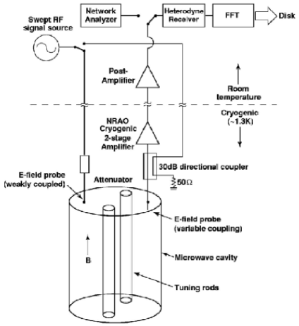
Figure 1: Schematic diagram of ADMX experiment including both the resonant cavity (which sits in the bore of a superconducting solenoid) and receiver electronics chain.

A schematic of the LLNL experiment, dubbed the Axion Dark Matter eXperiment (ADMX), can be seen in figure 1. The experiment consists of a cylindrical copper-plated steel cavity containing two axial tuning rods. These can be moved transversely from the edge of the cavity wall to its center allowing one to perturb the resonant frequency. The cavity itself is located in the bore of a superconducting solenoid providing a strong constant axial magnetic field. The electromagnetic field of the cavity is coupled to low-noise receiver electronics via a small adjustable antennaCavity_review . These electronics initially amplify the signal using two ultra-low noise cryogenic amplifiers arranged in series. The signal is then boosted again via a room temperature post-amplifier and injected into a double-heterodyne receiver. The receiver consists of an image reject mixer to reduce the signal frequency from the cavity resonance (hundreds of MHz - GHz) to an intermediate frequency (IF) of 10.7 MHz. A crystal bandpass filter is then employed to reject noise power outside of a 35 kHz window centered at the IF. Finally the signal is mixed down to almost audio frequencies (35 kHz) and analyzed by fast-Fourier-transform (FFT) electronics which compute a 50 kHz bandwidth centered at 35 kHz. Data is taken every 1 kHz or so by moving the tuning rods to obtain a new resonant $TM_{010}$ mode. In the next few sections we will expand on some of these components.

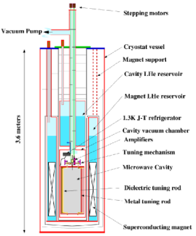
Figure 2: Overview of ADMX hardware including superconducting magnet and cavity insert.

3.1 Magnet

The main magnet for ADMX was designed to maximize the $B^{2}_{0}V$ contribution to the signal power (equation 2). It was determined that a superconducting solenoid would yield the most cost effective solution and its extremely large inductance (535 Henry) would have the added benefit of keeping the field very stable. The 6 ton magnet coil is housed in a 3.6 meter tall cryostat (see figure 2) with an open magnet bore allowing the experimental insert, with the cavity and its liquid helium (LHe) reservoir, to be lowered in. The magnet itself is immersed during operations in a 4.2 K LHe bath in order to keep the niobium-titanium windings superconducting. Generally the magnet was kept at a field strength of 7.6 T in the solenoid center (falling to approximately 70 % strength at the ends) but recently its been run as high as 8.2 T Cavity_review .

3.2 Microwave cavities

The ADMX experiment uses cylindrical cavities in order to maximize the axion conversion volume in the solenoid bore. They are made of a copper-plated steel cylinder with capped ends. The electromagnetic field structure inside a cavity can be found by solving the Helmholtz equation

$$\nabla^{2}\Phi+k^{2}\Phi=0$$ (9)

where the wavenumber $k$ is given by

$$k^{2}=\mu\epsilon\omega^{2}-\beta^{2}$$ (10)

and $\beta$ is the eigenvalue for the transverse (x,y) component Kinion_thesis . The cavity modes are the standing wave solutions to equation 9. The boundary conditions of an empty cavity only allow transverse magnetic (TM) modes ($\vec{B}_{z}=0$) and transverse electric (TE) modes ($\vec{E}_{z}=0$). Since the TE modes have no axial electric field one can see from equation 4 that they don’t couple at all to axions and we’ll ignore them for the moment. The $TM_{lmn}$ modes are three dimensional standing waves where $l=0,1,2...$ is the number of azimuthal nodes, $m=1,2,3...$ is the number of radial nodes and $n=0,1,2...$ is the number of axial nodes. The axions couple most strongly to the lowest order $TM_{010}$ mode.

The resonant frequency of the $TM_{010}$ mode can be shifted by the introduction of metallic or dielectric tuning rods inserted axially into the cavity. Metallic rods raise the cavity resonant frequency the closer they get to the center while dielectric rods lower it. In ADMX these rods are attached to the ends of alumina arms which pivot about axles set in the upper and lower end plates. The axles are rotated via stepper motors mounted at the top of the experiment (see figure 2) which swing the tuning rods from the cavity edge to the center in a circular arc. The stepper motors are attached to a gear reduction which translates a single step into a 0.15 arcsecond rotation, corresponding to a shift of $\sim$ 1 kHz at 800 MHz resonant frequency Cavity_review .

Figure 3: Resonant cavity with top flange removed. An alumina tuning rod can be seen at the bottom right and a copper tuning rod is in the upper left.

With the addition of metallic tuning rods TEM modes ($\vec{B}_{z}=\vec{E}_{z}=0$) can also be supported in the cavity. Like the TE modes they do not couple to the axions but they can couple weakly to the vertically mounted receiver antenna (due to imperfections in geometry, etc).

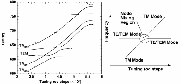
Figure 4: Mode structure of a cavity with two copper tuning rods. The left figure displays the frequencies of the resonant modes, measured via a swept rf signal, when one tuning rod is kept at the cavity edge while the other is moved toward the center. The right figure is a sketch of a mode crossing.

Figure 4 demonstrates how the various resonant modes shift as a copper tuning rod is moved from near the cavity wall toward the center. The TEM and TE modes are largely unaffected by the change in tuning rod position while TM modes rise in frequency as one of the copper rods moves toward the cavity center. This leads to regions in which a TM mode crosses a TE or TEM mode (referred to as mode mixing). These mode mixings (illustrated by the right part of figure 4) introduce frequency gaps which can not be scanned. As a result the cavity was later filled with LHe, which changed the microwave index of refraction to 1.027, thus lowering the mode crossings by 2.7% and allowed the previously unaccessible frequencies to be scanned.

A key feature of the resonant microwave cavity is its quality factor $Q$, which is a measure of the sharpness of the cavity response to external excitations. It is a dimensionless value which can be defined a number of ways including the ratio of the stored energy ($U$) to the power loss ($P_{L}$) per cycle: $Q=\omega_{0}U/P_{L}$. The quality factor (Q) of the $TM_{010}$ mode is determined by sweeping a radio (rf) signal through the weakly coupled antenna in the cavity top plate (see figure 1). Generally, the unloaded Q of the cavity is $\sim 2\times 10^{5}$ Cavity_review which is very near to the theoretical maximum for oxygen-free annealed copper at cryogenic temperatures. During data taking the insertion depth of the major antenna is adjusted to make sure that it matches the 50 $\Omega$ impedance of the cavity (called critically coupling). When the antenna is critically coupled half the microwave power in the cavity enters the electronics via the antenna while half is dissipated in the cavity walls. Overcoupling the cavity would lower the Q and thus limit the signal enhancement while undercoupling the cavity would limit the microwave power entering the electronics.

3.3 Amplifier and receiver

After the axion signal has been generated in the cavity and coupled to the major port antenna it is sent to the cryogenic amplifiers. The design of the first amplifier is especially important because its noise temperature (along with the cavity’s Johnson noise) dominates the rest of the system. This can be illustrated by following a signal from the cavity as it travels through two amplifiers in series. The power contribution from the thermal noise of the cavity at temperature $T_{c}$ over bandwidth $B$ is given by $P_{nc}=Bk_{B}T_{c}$ (where $k_{B}$ is Boltzmann’s constant). When this noise passes through the first amplifier, which provides gain $G_{1}$, the output includes the boosted cavity noise as well as extra power ($P_{N,A_{1}}$) from the amplifier itself. The noise from the amplifier appears as an increase in the temperature of the input source.

$$P_{1}=G_{1}Bk_{B}T_{c}+P_{N,A_{1}}=G_{1}Bk_{B}(T_{c}+T_{A_{1}})$$ (11)

If this boosted noise power (cavity plus first amplifier) is then sent through a second amplifier, with gain $G_{2}$ and noise temperature $T_{A_{2}}$, the power output becomes

$$P_{2}=G_{2}P_{1}+P_{N,A_{2}}=G_{2}(G_{1}Bk_{B}(T_{c}+T_{A_{1}}))+G_{2}Bk_{B}T_{A_{2}}$$ (12)

The combined noise temperature from the two amplifiers ($T_{A}$) can be found by matching equation 12 to that of a single amplifier, $P_{2}=G_{2}G_{1}Bk_{B}(T_{c}+T_{A})$, which gives

$$T_{A}=T_{A_{1}}+\frac{T_{A_{2}}}{G_{1}}$$ (13)

Thus one can see that, because of the gain $G_{1}$ of the first stage amplifier, its noise temperature dominates all other amplifiers in the series.

The current first stage amplifiers used in ADMX are cryogenic heterostructure field-effect transistors (HFETs) developed at the National Radio Astronomy Observatory (NRAO) specifically for the ADMX experiment Cavity_review ; NRAO . In these amplifiers electrons from an aluminum doped gallium arsenide layer fall into the GaAs two-dimensional quantum well (the FET channel). The FET electrons travel ballistically, with little scattering, thus minimizing electronic noise Physics_Today . Currently electronic noise temperatures of under 2 K have been achieved using the HFETs. In the initial ADMX data runs, now concluded, two HFET amplifiers were used in series, each with approximately 17 dB power gain, leading to a total first stage power gain of 34 dB. Each amplifier utilized 90 degree hybrids in a balanced configuration in order to minimize input reflections, thus providing a broadband match to the 50 $\Omega$ cavity impedance (see figure 5).

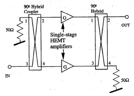
Figure 5: Schematic diagram of a balanced amplifier. Every time the signal crosses through the middle of a hybrid its phase is shifted by 90 degrees. Reflections back to the input destructively interfere while reflections to the upper left constructively interfere and are dumped into a 50 $\Omega$ terminator. Signals to the output are both shifted by 90 degrees and thus add constructively.

Though the amplifiers worked well in the high magnetic field just above the cavity it was determined during commissioning that they should be oriented such that the magnetic field was parallel to the HFET channel electron flow. This minimized the electron travel path and thus the noise temperature Cavity_review .

The signal from the cryogenic amplifiers is carried by coaxial cable to a low-noise room temperature post-amplifier, which added an additional 38 dB gain between 300 MHz - 1 GHz. Though the post-amplifiers noise temperature is 90 K its contribution relative to the cryogenic amplifiers (with 38 dB initial gain) is only 0.03 K (see equation 13). Including various losses the total gain from the cavity to the post-amplifier output is 69 dB Cavity_review .

After initial stages of amplification the signal enters the double-heterodyne receiver (essentially an AM radio). Figure 6 is a schematic of the receiver electronics. The first element is an image reject mixer which uses a local oscillator to mix the signal down to 10.7 MHz. This intermediate frequency (IF) is then sent through a programmable attenuator (used during room temperature testing so that the receiver electronics are not saturated). An IF amplifier then boosts the signal by another 20 dB before passing it by a weakly coupled signal sampler. The signal then passes through a crystal bandpass filter which suppresses noise outside a 30 kHz bandwidth center at 10.7 MHz. The signal is then boosted by an additional 20 dB before being mixed down to 35 kHz. The total amplification of the signals from the cavity is $\sim$ 106 dB General_art_1 .

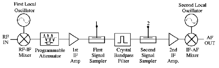
Figure 6: Receiver chain that mixes the signal down from the cavity $TM_{010}$ resonant frequency to 35 kHz.

Once the signal has been mixed down to the 35 kHz center frequency it is passed off to a commercial FFT spectrum analyzer and the power spectrum recorded. The entire receiver, including filter, is calibrated using a white-noise source at the input. During data collection the FFT spectrum analyzer takes 8 msec single-sided spectra (the negative and positive frequency components are folded on top of each other). Each spectrum consists of 400 bins with 125 Hz width spanning a frequency range of 10-60 kHz. After 80 seconds of data taking (with a fixed cavity mode) the 10,000 spectra are averaged together and saved as raw data. This is known as the medium resolution data.

In addition there is a high resolution channel to search for extremely narrow conversion lines from late infall non-thermal axions (as mentioned at the end of section 1). For this channel the 35 kHz signal is passed through a passive LC filter with a 6.5 kHz passband, amplified, and then mixed down to a 5 kHz center frequency. A single spectrum is then obtained by acquiring $2^{20}$ points in about 53 sec and a FFT is performed. This results in about $3.4\times 10^{5}$ points in the 6.5 kHz passband with a frequency resolution of 19 mHz.

4 Data analysis

The ADMX data analysis is split into medium and high resolution channels. The medium resolution channel is analyzed using two hypotheses. The first is a “single-bin” search motivated by the possibility that some of the axions have not thermalized and therefore would have negligible velocity dispersion, thus depositing all their power into a single power-spectrum bin. The second hypothesis utilizes a “six-bin” search which assumes that axions have a velocity dispersion of order $10^{-3}c$ or less (axions with velocities greater than $2\times 10^{-3}c$ would escape the halo). The six-bin search is the most conservative and is valid regardless of whether the halo axions have thermalized or not.

Since each 80 second long medium resolution spectra is only shifted by 1 kHz from the previous integration each frequency will show up in multiple spectra (given the 50 kHz window). As a result each 125 Hz bin is weighted according to where it falls in the cavity response function and co-added to give an effective integration time of $\sim$ 25 minutes per frequency bin. For the single-bin search individual 125 Hz bins are selected if they exceed an initial power-level threshold. This is set relatively low so a large number of bins are usually selected. These bins are then rescanned to achieve a similar signal-to-noise ratio and combined with the first set of data generating a spectra with higher signal to noise. The selection process is then repeated a number of times until persistent candidates are identified. These few survivors are then carefully checked to see if there are any external sources of interference that could mimic an axion signal. If all candidates turn out to be exterior radio interference the excluded axion couplings (assuming a specific dark matter density) can be computed from the near-Gaussian statistics of the single-bin data. For the six-bin search, all six adjacent frequency bins that exceed a set power-threshold are selected from the power spectra. The large number of candidates are then whittled down using the same iterations as the single-bin analysis. If no candidates survive the excluded axion couplings are computed by Monte Carlo Cavity_review .

From the radiometer equation (7) one can see that the search sensitivity can be increased if strong narrow spectral lines exist. The integration times for each tuning rod setting is around 60 seconds and the resulting Doppler shift from the Earth’s rotation leads to a spread of $\sim$ mHz in a narrow axion signal. Since the actual velocity dispersions of each discrete flow is unknown multiple resolution searches were performed by combining 19 mHz wide bins. These were referred to as $n$-bin searches, where $n=$ 1, 2, 4, 8, 64, 512 and 4096. Candidate peaks were kept if they were higher then a specified threshold set for that particular $n$-bin search. These thresholds were 20, 25, 30, 40, 120, 650 and 4500 $\sigma$, for increasing order of $n$. The initial search using the high resolution analysis took data between 478-525 MHz, corresponding to axion masses between 1.98 and 2.17 $\mu eV$. This search was made in three steps. First the entire frequency range was scanned in 1 kHz increments with the candidate axion peaks recorded. Next multiple time traces were taken of candidate peaks High_res . Finally persistent peaks were checked by attenuating or disconnecting various diagnostic coaxial cables leading into the cavity (see figure 1). If the signals were external interference they would decrease in power dramatically while an axion signal would remain unchanged Cavity_review . Further checks could be done by disconnecting the cavity from the receiver input and replacing it with an antenna to see if the signal persisted.

If a persistent candidate peak is found which does not have an apparent source from external interference a simple check would be to turn off the magnetic field. If the signal disappears it would be a strong indication that it was due to axions and not some unknown interference. So far, though, all candidates have been identified with an external source.

5 Results

So far no axions have been detected in any experiment. ADMX currently provides the best limits from microwave cavity experiments in the lowest mass range (most plausible if axions are the major component to the dark matter). Both the medium resolution data and the high resolution data yield exclusion plots in either the coupling strength of the axion (assuming a halo density of $\rho_{a}=0.45\;GeV/cm^{3}$) or in the axion halo density (assuming a specific DFSZ or KSVZ coupling strength). Results from the medium resolution channel Med_res can be seen in figure 7 and the high resolution results High_res can be seen in 8. Both of the results are listed at 90 % confidence level.

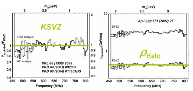
Figure 7: Results from the medium resolution channel Med_res . The figure to the left is the exclusion plot for power in a thermalized spectrum assuming a halo density of $\rho_{a}=0.45\;GeV/cm^{3}$. The figure to the right is the fractional dark matter halo density excluded as axions for two different axion models.

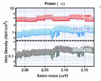
Figure 8: High resolution limits given different axion couplings High_res . This shows that the current high resolution channel is sensitive to fractional halo densities ($\approx$ 30%) if the axions couple via the KSVZ model. If they couple via the DFSZ model the experiment is not yet sensitive to the maximum likelihood halo density ($\rho_{a}\sim 0.45\;GeV/cm^{3}$), but would be sensitive to a single line with twice that density.

6 Future developments

In order to carry out a definitive search for axion dark matter various improvements to the detector technology need to be carried out. Not only do the experiments need to become sensitive enough to detect even the most pessimistic axion couplings (DFSZ) at fractional halo densities but they must be able to scan relatively quickly over a few decades in mass up to possibly hundreds of GHz. The sensitivity of the detectors (which is also related to scanning speed) is currently limited by the noise in the cryogenic HFET amplifiers. Even though they have a noise temperature under 2 K the quantum limit (defined as $T_{Q}\sim h\nu/k$) is almost two orders of magnitude lower (25 mK at 500 MHz). To get down to, or even past, this quantum limit two very different technologies are being developed. The first is the implementation of SQUIDs (Superconducting Quantum Interference Devices) as first stage cryogenic amplifiers. The second uses Rydberg-atoms to detect single microwave photons from axion conversions in the cavity.

Though both techniques will lead to vastly more sensitive experiments they will still be limited in their mass range. Currently all cavity experiments have been limited to the $2-20\mu eV$ range, mostly due to the size of resonant cavities. For a definitive search the mass range must be increased by a factor of 50 which requires new cavity designs that increase the resonant frequency while maintaining large enough detection volumes. Detectors that work at these higher frequencies also need to be developed.

6.1 SQUID amplifiers

The next generation of the ADMX experiment will use SQUID amplifiers to replace the first stage HFETs. SQUIDs essentially use a superconducting loop with two parallel Josephson junctions to enclose a total amount of magnetic flux $\Phi$. This includes both a fixed flux supplied by the bias coil and the signal flux supplied by an input coil. The phase difference between the currents on the two sides of the loop are affected by changing $\Phi$ resulting in an interference effect similar to the two-slit experiment in optics Kinion_thesis . Essentially the SQUID will act as flux to voltage transducers as illustrated in figure 9.

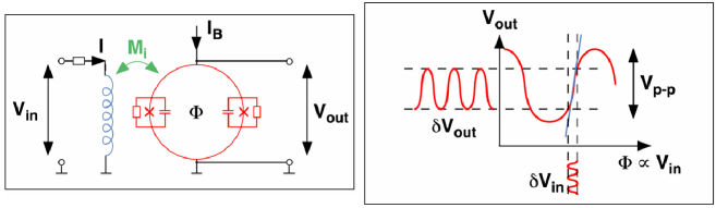
Figure 9: Essentials of a SQUID microwave detector. The left figure is a schematic of the SQUID device coupling to the input signal which is converted into magnetic flux. The right figure shows how biasing the flux allows for amplification.

Most SQUIDs are built using the Ketchen and Jaycox design Ketchen , in which the SQUID loop is an open square washer made of niobium (Nb). The loop is closed by a separate Nb electrode connected to the washer opening on either side by a Josephson junction and external shunt resistors. A spiral input coil is placed on top of the washer, separated by a layer of insulation. The original designs in which input signals were coupled into both ends of the coil tended to only work below about 200 MHz due to parasitic capacitance between the coil and the washer at higher frequencies. This was solved by coupling the input signal between one end of the coil and the SQUID washer, which would act as a ground plane to the coil and create a microstrip resonator (see figure 10). This design has been tested successfully up to 3 GHz Kinion_thesis .

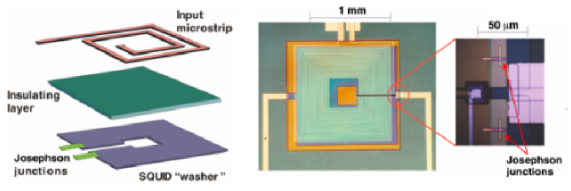
Figure 10: Diagram and picture of microstrip resonator SQUIDs to be used in ADMX upgrade.

Unlike the HFETs, whose noise temperature bottoms out at just under 2 K regardless of how cold the amplifiers get, the SQUIDs noise temperature remains proportional to the physical temperature down to within 50% of the quantum limit. The source of this thermal noise comes from the shunt resistors across the SQUID’s Josephson junctions and future designs that minimize this could push the noise temperature even closer to the quantum limit Physics_Today .

Currently the ADMX experiment is in the middle of an upgrade in which SQUIDs will be installed as first stage cryogenic amplifiers. This should cut the combined noise temperature of the cavity + electronics in half allowing ADMX to become sensitive to half the KSVZ coupling (with the same scanning speed as before). Due to the SQUIDs’ sensitivity to magnetic fields this upgrade includes an entire redesign in which a second superconducting magnet is being installed in order to negate the main magnet’s field around the SQUID amplifiers. Data taking is expected to begin in the first half of 2007 and run for about a year. Future implementations of ADMX foresee using these SQUID detectors with a dilution refrigerator to set an operating temperature of $\sim$ 100 mK, allowing sensitivity to DFSZ axion couplings to be achieved with 5 times the scanning rate the current HFETs take to reach KSVZ couplings.

6.2 Rydberg-atom single-quantum detectors

One technique to evade the quantum noise limit is to use Rydberg atoms to detect single photons from the cavity. A Rydberg atom has a single valence electron promoted to a level with a large principal quantum number $n$. These atoms have energy spectra similar in many respects to hydrogen, and dipole transitions can be chosen anywhere in the microwave spectrum by an appropriate choice of $n$. The transition energy itself can be finely tuned by using the Stark effect to exactly match a desired frequency. That, combined with the Rydberg atom’s long lifetime and large dipole transition probability, make it an excellent microwave photon detector.

An experimental setup utilizing this technique called CARRACK has been assembled in Kyoto, Japan Cavity_review ; Kyoto_1 and a schematic can be seen pictured in figure 11. The axion conversion cavity is coupled to a second “detection” cavity tuned to the same resonant frequency $\nu$. A laser excites an atomic beam (in this case rubidium) into a Rydberg state ($|0>\rightarrow|n>$) which then traverses the detection cavity. The spacing between the energy levels is adjusted to $h\nu$ using the Stark effect and microwave photons from the cavity can be efficiently absorbed by the atoms (one photon per atom, $|ns>\rightarrow|np>$). The atomic beam then exits the cavity and is subjected to selective field ionization in which electrons from atoms in the higher energy state ($|np>$) get just enough energy to be stripped off and detected Physics_Today .

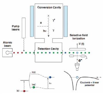
Figure 11: Schematic of single photon microwave detection utilizing Rydberg atoms.

Currently the Kyoto experiment has measured cavity emission at 2527 MHz down to a temperature of 67 mK, a factor of two below the quantum limit at that frequency, and is working to reach the eventual design goal of 10 mk Kyoto_1 . This would be the point in which the cavity blackbody radiation would become the dominant noise background. One deficiency of the Rydberg atom technique is that it can’t detect structure narrower than the bandpass ($\Delta E/E$) of the cavity (generally $\sim 10^{-5}$). As a result it is insensitive to axion halo models that predict structure down to $\Delta E/E\sim 10^{-11}$, an area in which the ADMX high resolution channel, utilizing microwave amplifiers, can cover. Despite this Rydberg atom detectors could become very useful tools for halo axion detection in the near future.

6.3 Challenge of higher frequencies

Current microwave cavity technology has only been able to probe the lowest axion mass scale. In order to cover the entire range up to the exclusion limits set by SN 1987a of $m_{a}\leq meV$ new cavity and detection techniques must be investigated which can operate up to the 100 GHz range. The resonant cavity frequency essentially depends on the size the cavity and the resonant mode used. The $TM_{010}$ mode has by far the largest form factor ($C\sim 0.69$) of any mode and all other higher frequency modes have much smaller or identically zero form factors. The single 50 cm diameter cavity used in the initial ADMX experiments had a central resonant frequency ($TM_{010}$) of 460 MHz and radial translation of metallic or dielectric tuning rods could only raise or lower that frequency by about $\pm 50\%$ Cavity_review . Smaller cavities could get higher frequencies but the rate of axion conversions would go down as the cavity volume decreased.

In order to use the full volume of the magnet with smaller cavities it was determined that multiple cavities could be stacked next to each other and power combined. As long as the de Broglie wavelength of the axions is larger than the total array individual cavities tuned to the same frequency can be summed in phase. Typical axion de Broglie wavelengths are $\lambda_{dB}\sim 10m-100m$ which means they drive the $\sim 1m$ cavity volume coherently. Data taken using a four cavity array in ADMX reached KSVZ sensitivity Kinion_thesis over a small mass range (see figure 12). These initial tests had difficulties getting the piezoelectric motors working trouble free in the magnetic and cryogenic environment. Since those tests the technology has advanced to the point in which it may be feasible to create larger sets of smaller cavity areas.

To reach even higher frequencies ideas have been raised to use resonators with periodic arrays of metal posts. Figure 12 shows the electric field profile of one possible array using a 19 post hexagonal pattern. Mounting alternating posts from the cavity top and the bottom and translating them relative to each other allow the resonant frequency to be adjusted by 10% or so. The possibility of using such cavities, or other new cavity geometries, is an active area of research and progress needs to be made before the full axion mass range can be explored.

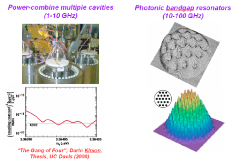
Figure 12: Outline of possible cavity concepts to explore higher axion masses. The left figure includes both a picture of the 4 cavity array and its corresponding exclusion plot over the limited mass range it took data. The right figure includes field maps for multiple posts inserted in a cavity.

7 Summary, conclusions

Experimentally the axion is a very attractive cold dark matter candidate. Its coupling to photons ($g_{\gamma}$) for several different models all fall within about an order of magnitude in strength and its mass scale is currently confined to a three decade window. This leaves the axion in a relatively small parameter space, the first two decades or so of which is within reach of current or near future technology.

The ADMX experiment has already begun to exclude dark matter axions with KSVZ couplings over the lowest masses and upgrades to SQUID amplifiers and a dilution refrigerator could make ADMX sensitive to DFSZ axion couplings over the first decade in mass within the next three years. Development of advanced Rydberg-atom detectors, along with higher frequency cavities geometries, could give rise to the possibility of a definitive axion search within a decade. By definitive we mean a search which would either detect axions at even the most pessimistic couplings (DFSZ) at fractional halo densities over the full mass range, or rule them out entirely.

It should be noted that if the axion is detected it would not only solve the Strong-CP problem and perhaps the nature of dark matter but could offer a new window into astrophysics, cosmology and quantum physics. Details of the axion spectrum, especially if fine structure is found, could provide new information of how the Milky Way was formed. The large size of the axions de Broglie wavelength ($\lambda_{a}\sim 10m-100m$) could even allow for interesting quantum experiments to be performed at macroscopic scales. All of these tantalizing possibilities, within the reach of current and near future technologies, makes the axion an extremely exciting dark matter candidate to search for.

8 Acknowledgments

This work was supported under the auspices of the U.S. Department of Energy under Contract W-7405-Eng-48 at Lawrence Livermore National Laboratory.

References

- [1] D.N. Schramm and M. S. Turner. Big-bang nucleosynthesis enters the precision era. Reviews of Modern Physics, 70:303–318, January 1998.
- [2] M. Tegmark et al. Cosmological parameters from SDSS and WMAP. Physical Review D, 69:103501(26), 2004.
- [3] F. Zwicky. On the Masses of Nebulae and of Clusters of Nebulae. Helvetica Physica Acta, 6:110–127, 1933.
- [4] G. Jungman, M. Kamionkowski, and K. Griest. Supersymmetric Dark Matter. Physics Reports, 267:195–373, 1996.
- [5] D.N. Spergel et al. First-Year Wilkinson Microwave Anisotropy Probe (WMAP) Observations: Determination of Cosmological Parameters. Astrophysical Journal Supplement Series, 148(1):175–194, 2003.
- [6] F. De Paolis et al. The case for a baryonic dark halo. Physical Review Letters, 74:14–17, January 1995.
- [7] C. Alcock et al. The MACHO Project: Microlensing results from 5.7 years of Large Magellanic Cloud observations. The Astrophysical Journal, 542:281–307, 2000.
- [8] C. Afonso et al. Limits on galactic dark matter with 5 years of EROS SMC data. Astronomy and Astrophysics, 400:951–956, March 2003.
- [9] J.T. Kleyna et al. First clear signatures of an extended dark matter halo in the Draco Dwarf Spheroidal. Astrophysical Journal Letters, 563:115–118, 2001.
- [10] J.R. Primack. Dark Matter and Structure Formation in the Universe. Proceedings of Midrasha Matematicae in Jerusalem: Winter School in Dynamic Systems, 1997.
- [11] E.I. Gates, G. Gyuk, and M.S. Turner. The Local Halo Density. The Astrophysical Journal, 449:L123–L126, August 1995.
- [12] P.G. Harris et al. New experimental limit on the electric dipole moment of the neutron. Physical Review Letters, 82:904–907, 1999.
- [13] J.E. Kim. Weak-Interaction singlet and strong CP invariance. Physical Review Letters, 43:103–107, July 1979.
- [14] M.A. Shifman, A.I. Vainshtein, and V.I. Zakharov. Can confinement ensure natural CP invariance of strong interactions. Nuclear Physics B, 166:493–506, 1980.
- [15] A.R. Zhitnitskii. . Soviet Journal of Nuclear Physics, 31:260–, 1980.
- [16] M. Dine, W. Fischler, and M. Srednicki. A simple solution to the strong CP problem with a harmless axion. Physics Letters B, 104:199–202, 1981.
- [17] S. Weinberg. A new light boson. Physical Review Letters, 40:223–226, 1978.
- [18] F. Wilczek. Problem of strong P and T invariance in the presence of instantons. Physical Review Letters, 40:279–282–, 1978.
- [19] R. Bradley et al. Microwave cavity searches for dark-matter axions. Reviews of Modern Physics, 75:777–817, 2003.
- [20] P. Sikivie. Evidence for ring caustics in the Milky Way. Physics Letters B, 567:1–8, June 2003.
- [21] P. Sikivie. Experimental Test of the ”Invisible” Axion. Physical Review Letters, 51:1415–1417, October 1983.
- [22] Pioneer 10 Project Manager Larry Lasher, 2005. Private Communication.
- [23] R.H. Dicke. The Measurement of Thermal Radiation at Microwave Frequencies. The Review of Scientific Instruments, 17:268–275, July 1946.
- [24] S.J. Asztalos et al. Improved rf cavity search for halo axions. Physical Review D, 69:011101(5), January 2004.
- [25] S. DePanfilis et al. Limits on the abundance and coupling of cosmic axions at . Physical Review Letters, 59:839–842, August 1987.
- [26] C. Hagmann et al. Results from a search for cosmic axions. Physical Review D, 42:1297–1300, August 1990.
- [27] Darin Kinion. First results from a multiple-microwave-cavity search for dark-matter axions. PhD dissertation, UC Davis, Physics Department, 2001.
- [28] E. Daw and R. F. Bradley. Effects of high magnetic fields on the noise temperature of a heterostructure field-effect transistor low-noise amplifier. Journal of Applied Physics, 82(4):1925–1929, August 1997.
- [29] K. van Bibber and L. Rosenberg. Ultrasensitive searches for the axion. Physics Today, pages 30–35, August 2006.
- [30] S. Asztalos et al. Large-scale microwave cavity search for dark-matter axions. Physical Review D, 64:092003(28), November 2001.
- [31] L.D. Duffy et al. High Resolution Search for Dark-Matter Axions. Physical Review D, 74:012006(11), July 2006.
- [32] M.B. Ketchen and M.B. Jaycox. Ultra-low-noise tunnel junction dc SQUID with a tightly coupled planar input coil. Applied Physics Letters, 40:736–738, April 1982.
- [33] M. Tada et al. Single-photon detection of microwave blackbody radiatons in a low-temperature resonant-cavity with high Rydberg atoms. Physics Letters A, 349:488–493, October 2006.