Flavor Tagging at Tevatron incl. calibration and control

Abstract

This report summarizes the flavor tagging techniques developed at the CDF and DØ experiments. Flavor tagging involves identification of the $B$ meson flavor at production, whether its constituent is a quark or an anti-quark. It is crucial for measuring the oscillation frequency of neutral $B$ mesons, both in the $B^{0}$ and $\mathrm{B}^{0}_{s}$ system. The two experiments have developed their unique approaches to flavor tagging, using neural networks, and likelihood methods to disentangle tracks from $b$ decays from other tracks. This report discusses these techniques and the measurement of $B^{0}$ mixing, as a means to calibrate the taggers.

1 INTRODUCTION

Flavor tagging is important in studies of neutral $B$ meson mixing and CP violation in the $B$ system. At hadron colliders, because of minimum bias events and multiple interactions per crossing, the background level is higher as compared to the more cleaner environment at $e^{+}e^{-}$ colliders. Also, at hadron colliders the $b$-jets may not always be well separated (as in the case of $g\rightarrow b\bar{b}$), while at $\mathrm{e}^{+}e^{-}$ colliders, one gets well balanced and separated jets. Therefore, in order to identify $b$-jets or decays one needs sophisticated techniques to achieve a good efficiency and purity of the tags. Broadly speaking, flavor tagging methods can be categorized into Opposite Side Tagging (OST) and Same Side Tagging (SST) [1]. In the case of OST, one uses the decay products of the opposite $B$ in the event, and since the $B$ mesons are produced in pairs in a $b\bar{b}$ event, the $B$ flavor of the tag side is ideally opposite to the $B$ flavor of the decay side (The $B$ meson which is fully or partially reconstructed is referred to as the “decay” or “reconstruction” side $B$ meson). The tag side $B$ meson however could oscillate if it was neutral, independent of the reconstruction side $B$ meson and therefore in such a case the tag would incorrect. OST flavor taggers are sub-categorized into (i) Lepton taggers, where one exploits the charge correlation of the lepton and the quark flavor in semileptonic $b$ decays, (ii) Jet charge taggers, where one use the fact that the kinematically weighted charge of the $b$-jet is correlated with the charge of the $b$, and (iii) Opposite Side Kaon Tagger (OSKT), where one exploits the correlation of the charge of the kaon with the $B$ flavor in the decay chain $b\rightarrow c\rightarrow XK^{-}$. In the case of SST, one utilizes the charge correlation of the fragmentation tracks produced on the same side as the “reconstructed” $B$. For SST the wrong sign contribution due to the “tag” $B$ meson oscillating is absent, and it has a high efficiency, but it has a somewhat worse purity than the OST tagger, as it is difficult to identify the correct fragmentation track from a large number of decay product tracks.

Flavor taggers are optimized to obtain high efficiencies ($\varepsilon$) and purities, where $\varepsilon$ is defined as the fraction of reconstructed events ($N_{\rm{tot}}$) that are tagged ($N_{\rm{tag}}$): $\varepsilon=N_{\rm{tag}}/N_{\rm{tot}}$. The term dilution ($\cal{D}$) is more commonly used, which is related to the purity, $P$, as ${\cal{D}}=2P-1$ and is defined as the normalized difference of correctly and wrongly tagged events: ${\cal{D}}=\frac{N_{\rm{cor}}-N_{\rm{wr}}}{N_{\rm{cor}}+N_{\rm{wr}}}=\frac{N_{\rm{cor}}-N_{\rm{wr}}}{N_{\rm{tag}}}$ where, $P=N_{\rm{cor}}/N_{\rm{tag}}$. The terms “correctly” and “wrongly” refer to the determination of the decay $B$ meson flavor. The effective tagging power of a tagging algorithm is given by $\varepsilon{\cal{D}}^{2}$ and the goal is to maximize this quantity.

2 CDF AND DØ DETECTOR

Leptons from $B$ decays have low momenta as compared to leptons from top or electroweak decays, and require special treatment to identify them. The complexity of lepton identification needed depends on the detector. The CDF detector has a muon coverage up-to $|\eta|\leq 1.5$ and the DØ detector has a muon coverage up-to $|\eta|\leq 2.0$ in RunII. At CDF, the Central muon chamber (CMU) is situated just outside the hadron calorimeter. Hence, the fake rate from punchthroughs, and decay in flights (DIF’s) from kaons and pions decaying into muons, for the CMU muons is high. Another layer of muon chambers was therefore installed further up, for the RunII phase, which is acronymed as CMP. The rates of punch-through and DIF’s are studied in data. The central muon detectors at DØ are proportional drift tubes (PDT’s) located in the pseudo-rapidity range of $0.0<|\eta|<1.0$ and mini-drift tubes (MDT’s) between $1.0<|\eta|<2.0$. Both the central and forward detectors consist of 3 layers, with the first layer just outside the hadron calorimeter and the other two layers lying outside the toroid. Muons at DØ have negligible punchthrough background after requiring that it passes the toroid.

The CDF calorimeter is a sampling calorimeter consisting of layers of scintillators and lead. There is a position detector at shower maximum, at about 6 radiation lengths ($X_{0}$), which is composed of orthogonal strips and wires, and provides measurement in the $x$ and $z$ direction. Besides this, a central pre-radiator at about 1 $X_{0}$ is useful as an additional layer for identifying electrons, especially low momentum electrons which can start showering much before the EM calorimeter. This was a gas wire chamber in the RunIIa phase and is now replaced by scintillators in the RunIIb phase. The DØ calorimeter is a primarily liquid-argon/uranium sampling calorimeter, covering up-to $|\eta|<4$. The central preshower situated at $\approx$ 1 $X_{0}$, is made of three concentric cylindrical layers of triangular cross-section scintillator strips, with wavelength shifting fiber (WLS) readout.

More details on the CDF and DØ detector can be found in ref. [2] and [3] respectively.

3 OPPOSITE SIDE TAGGING

3.1 Soft lepton identification

For identifying muons, CDF developed a muon likelihood function, to disentangle background coming from punchthroughs and DIF’s, which is especially problematic in the CMU. The muon ID variable probability density functions (pdf’s) were developed from data, using signal muons from $J/\Psi\rightarrow\mu^{+}\mu^{-}$ and fakes from $K^{0}_{S}\rightarrow\pi^{+}\pi^{-}$ and other modes. The energy deposit in the hadron calorimeter for signal and fakes can be seen in Fig. 1.

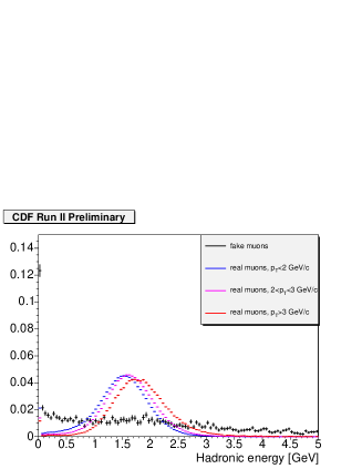
Figure 1: Energy deposit in the hadron calorimeter for fakes and signal muons at CDF. The black dots come from fakes peaking at 0, while real muons deposit around 1.5-2.0 GeV depending on their $p_{T}$, consistent with a minimum ionizing particle.

At DØ, simple cuts are used, as there is negligible punchthrough after requiring that the muon must pass the toroid.

The standard electron reconstruction is based on calorimeter clusters, relying on the characteristic transverse and longitudinal shapes of electromagnetic showers and is usually designed for high $p_{T}$ electrons. The leptons in $B$ decays have low momenta and could be non-isolated and within the b-jet. For low $p_{T}$ electrons, in order to achieve a higher purity and to remove contamination from nearby tracks, one starts with the track and extrapolates it to the calorimeter and it suffices to use a fewer number of towers to form a narrower cluster. DØ uses simple cuts on the electron ID quantities while CDF uses a likelihood variable. To optimize the cuts or to develop the likelihood, electrons from photon conversions $\gamma\rightarrow\mathrm{e}^{+}e^{-}$ as signal and $K^{0}_{S}\rightarrow\pi^{+}\pi^{-}$ are used for the fakes. Electrons from photon conversions have a very similar $p_{T}$ spectrum as electrons from $b$-decays. The ratio of energy deposited in the electromagnetic calorimeter to the momentum of the track for the DØ experiment can be see in Fig. 2

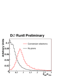
Figure 2: The fraction of energy deposited in the electro-magnetic calorimeter to the momentum of the track.

3.2 OST development at CDF

CDF uses a lepton and displaced track trigger, called Silicon Vertex Trigger (SVT) at level2 to collect a $b$-enriched inclusive, high statistics sample to calibrate the lepton taggers. To enhance the $b$ component further, the invariant mass of the lepton and displaced track system $M_{l+SVT}$ is required to be consistent with a $B$ candidate, using the cut, $2<M_{l+SVT}<4$ GeV. Furthermore, true $B$ decays should have a positively displaced signed impact parameter $\delta$, where $\delta=|d_{0}|sign(d_{0}\cdot p_{l+SVT})$, $d_{0}$ being the impact parameter of the track. Therefore, a background subtraction is done, and the sample with negative impact parameter is subtracted from the sample with positive signed impact parameter (See Fig. 3). However, since this sample is inclusive of all $B$ decays, the trigger side can mix and undergo sequential decays and there are also fake leptons, which means that the sign of the lepton does not give the correct $B$ meson flavor at the decay side. Thus, the “true” tagger dilution is given by the “raw” tagger dilution/”trigger” side dilution.

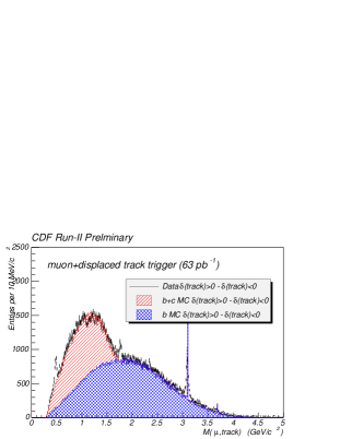
Figure 3: The invariant mass distribution for $l+SVT$ sample with the negative impact parameter background component subtracted. The $b$ and $c$ components from MC are also superimposed

3.2.1 Lepton tagging

The sign of the $B$ flavor on the “decay” side is given by the trigger lepton in the $l+SVT$ sample. Tag leptons (muon or electron) with $p_{T}>2GeV$ are searched for, on the opposite side using the soft lepton identification algorithms as described in section 3.1. Only electrons in the range $|\eta|\leq 1$ are used. The dilution is then parametrized as a function of the transverse momentum of the tag lepton w.r.t the tag lepton jet ($p_{T}^{\rm rel}$) and the electron or muon likelihood cut, to provide an event-by-event dilution [4].

3.2.2 Jet charge tagging

The jet charge tag starts with forming track based jets. Each of the tracks in the jet are assigned a “b”-ness probability using a neural network, called a TrackNet probability. Some of the track properties used as inputs to the neural network are the impact parameter significance, the signed impact parameter, the transverse momentum, and others. To select the single best $b$-jet in the presence of multiple jets, the jets are fed to a neural network, and the jet with the highest NN probability ($P_{nn}$) is chosen. The jet charge is calculated as $Q_{jet}=\frac{\sum q_{i}p_{T}^{i}(1+t_{i})}{\sum p_{T}^{i}(1+t_{i})}$, where $t_{i}$ is the NN probability for the track. The jets are then divided into three categories based on the presence of a secondary vertex or the number of tracks with high NN prob., and for each class the dilution is derived as a function of $|Q_{jet}|*P_{nn}$. The NN probability for all the jets and the dilution calibration for class 1 jets can be seen in Fig. 4. The results are summarized in table 1.

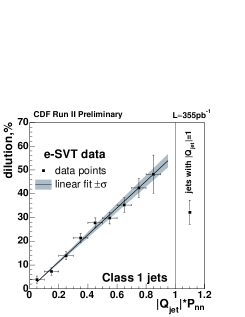
Figure 4: The dilution as a function of $|Q_{jet}|*P_{nn}$ for class 1 jets in the electron+displaced track trigger sample.

3.2.3 Opposite side kaon tagging

CDF utilizes dE/dx in the tracker and time-of-flight (TOF) information to identify kaons. The following results are found for OSKT [4]: $\varepsilon=18.11\pm 0.07\%$ and $\varepsilon{\cal{D}}^{2}=0.229\pm 0.016\pm 0.001(\%)$

3.3 OST development at D0

At DØ one collects samples using an inclusive muon trigger. Then, $B^{+}\rightarrow D^{0}\mu^{+}\nu X$ decays are reconstructed and used for the development of the tagger. (Charge conjugated states are implied throughout the note). In this sample, the muon charge gives the flavor of the reconstruction side $B$ since charged $B$’s do not oscillate. This sample has a small contribution from $B^{0}$ decays but by requiring a small decay length of the $B$ candidate, the sample is composed of $98\%$ of the decays from $B^{+}$ mesons. On the opposite side then, one can construct p.d.f’s for tag variables that distinguish between $b$ and $\bar{b}$, the flavor information being given by the sign of the muon in this sample’s case. For n discriminating variables, therefore the combined tagging variable $r$ is defined as: $r=\prod_{i=1}^{n}r_{i}$, where $r_{i}$ is given by the ratio of the p.d.f’s for a $b$ and a $\bar{b}$ quark. A more convenient tagging variable is defined as: $d=\frac{1-r}{1+r}$, which ranges between $-1$ and $1$, and an event with $d>0$ is tagged as a $b$ quark and with $d<0$ as a $\bar{b}$ quark. A higher $|d|$ value corresponds to higher $b$-ness of the tag. Specifically, for each event with an identified muon on the opposite side, the discriminating variables, muon jet charge $Q_{J}^{\mu}$, and the secondary vertex charge $Q_{SV}$ are used to construct a muon tagger. For each event without a muon but with an identified electron, the electron jet charge $Q_{J}^{e}$ and the secondary vertex charge $Q_{SV}$ are used to construct an electron tagger. Finally, for events without a muon or an electron but with a reconstructed secondary vertex, the secondary vertex charge $Q_{SV}$, and the event jet charge $Q_{EV}$ are used to construct a secondary vertex tagger. The resulting distribution of the tagging variable $d$ for the combination of all three taggers, called the combined tagger, is shown in Fig. 5. More details can be found in Ref. [5].

Figure 5: Normalized distributions of the combined tagging variable $d$. $q(b^{\rm rec})$ is the charge of the $b$ quark from the reconstruction side.

4 SAME SIDE TAGGING AT CDF

To develop the same side tagging, especially in the case of $\mathrm{B}^{0}_{s}$ mesons, one has to rely on Monte Carlo (MC) since the tagging is species dependent and in the case of $B^{0}$ the fragmentation track is a pion while in the case of $\mathrm{B}^{0}_{s}$ its a kaon. Hence, one needs to achieve a good data-MC agreement in the high statistics $B^{0}$ and $B^{+}$ modes, and then study the systematic uncertainties of the prediction of the tagger performance from MC samples for the $\mathrm{B}^{0}_{s}$ data. Of importance to this analysis is the use of particle identification systems like the TOF detector, and the use of energy loss (dE/dx) in the drift chamber to distinguish between kaon and pion tracks, in particular. An effective tagging power of $4.0^{+0.9}_{-1.2}\%$ is found [4].

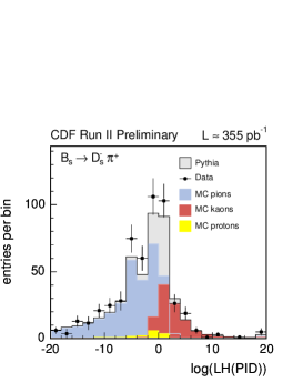
Figure 6: Data-MC comparison in $\mathrm{B}^{0}_{s}$ decays for kaon PID variable. where $log(LH(PID))=log\frac{P_{TOF}(K)P_{dEdx}(K)}{{f_{p}}{P_{TOF}}(p){P_{dEdx}}(p)+{f_{\pi}}{P_{TOF}}(\pi){P_{dEdx}}(\pi)}$ and $f_{p}=0.1$ and $f_{\pi}=0.9$ are a priori probabilities of background composition and $P_{TOF}$ and $P_{dE/dx}$ are determined from pure samples.

5 $B^{0}$ MIXING AND TAGGER CALIBRATION

$B^{+}\rightarrow\bar{D}^{0}\mu^{+}X$ and $B^{0}\rightarrow D^{*-}\mu^{+}X$ samples are used for measuring $B^{0}$ mixing and for tagger calibration. The sample composition of $B$ meson species and $c\bar{c}$ events contributing to the final states are obtained from realistic simulated events.

5.1 Results from DØ

The asymmetries given by the difference of opposite-sign and same-sign tagged events are obtained by fitting the $D^{0}$ mass distribution in the $D^{0}$ and $D^{*}$ samples as a function of the visible proper decay length ($x^{M}$) of the D+$\mu$ candidate. $x^{M}$ is related to the real $B$ decay length as $Kx^{M}=c\tau_{B}$, where K-factor is evaluated from MC as the ratio of the transverse momenta of the $D+\mu$ candidate and the generated B meson. The asymmetries can then be fitted in a binned $\chi^{2}$ fit to extract $\mathrm{\Delta{m}_{d}}$ and the tagger dilution ${\cal{D}}$. The samples are divided into 5 sub-samples of low to high purity in the tag variable $|d|$ and fitted in a combined fit to extract the ${\cal{D}}$’s as a function of $|d|$ thus providing an event-by-event dilution. This calibration curve is then used for $\mathrm{B}^{0}_{s}$ mixing studies. The asymmetry fit in one of the 5 $|d|$ bins can be seen in Fig. 7. More details can be found in Ref. [5]. Summing the individual tagging powers of all $|d|$ bins after the fit, one obtains an effective tagging power of $\varepsilon{\cal D}^{2}=[{2.48\pm 0.21~{}{\rm(stat.)}}^{+0.08}_{-0.06}~{}{\rm(syst)}]~{}\%$. The fraction $f_{c\bar{c}}$ which is constrained to be the same for all subsamples is found to be $f_{c\bar{c}}=(2.2\pm 0.9)\%$, and the $B^{0}$ mixing parameter $\mathrm{\Delta{m}_{d}}$ is found to be $\mathrm{\Delta{m}_{d}}=0.506\pm 0.020(stat.)\pm 0.016(syst.)~{}\mbox{ps}^{-1}$ in good agreement with world average value of $0.507\pm 0.005~{}{\rm ps}^{-1}$ [6].

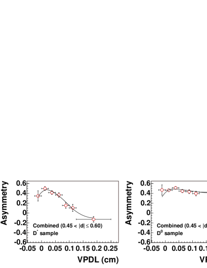
Figure 7: Asymmetries obtained in the $D^{0}$ and $D^{*}$ data samples with the combined tagger as a function of visible proper decay length (VPDL) in one of the $|d|$ bins at the DØ experiment. The circles are data and the fit is superimposed.

5.2 Results from CDF

CDF obtains the dilution calibration from the inclusive lepton+SVT samples (See Sec.3.2.1 and 3.2.2) and introduces a scale factor to describe the differences in dilution for the individual decay modes considered. Using a sample corresponding to an integrated luminosity of $355\,{\rm pb}^{-1}$, an unbinned likelihood simultaneous fit to both mass and lifetime is performed and a $\mathrm{\Delta{m}_{d}}$ of $0.536\pm 0.028\pm 0.006~{}\mbox{ps}^{-1}$ and an $\varepsilon{\cal{D}}^{2}=(1.55\pm 0.16\pm 0.05)\%$ is found in the case of hadronic decays, and using a similar method and an integrated luminosity of $1\,{\rm fb}^{-1}$, a $\mathrm{\Delta{m}_{d}}=0.509\pm 0.010\pm 0.016~{}\mbox{ps}^{-1}$ and $\varepsilon{\cal{D}}^{2}=(1.54\pm 0.05)\%$ is obtained in the case of semileptonic decays [4].

6 FLAVOR TAG SUMMARY

Overall tagging performances for the two experiments is summarized in Table 1. For the individual tagger numbers quoted for DØ a cut of $|d|>0.3$ was used. The DØ combined tagger uses events with $|d|<0.3$, hence overall effective tagging power is higher. CDF also used a neural network method to combine the individual taggers and finds an increase in OST effective tagging power from $1.5\%$ to $1.8\%$ [4]. After demonstrating a consistent measurement of $B^{0}$ mixing, the flavor tagging calibration can then be used for $\mathrm{B}^{0}_{s}$ mixing studies and was used to obtain the $\mathrm{B}^{0}_{s}$ mixing results at the two experiments [7], [8].

Table 1: Flavor Tag Summary at the Tevatron. Here, the soft muon and soft electron taggers are denoted SMT and SET respectively. The three categories of Jet Charge Taggers (JQT) (See Sec. 3.2.2), jets with an associated secondary vertex, highly displaced tracks content and the rest of the jets, are referred to as JVX, JJP and JPT. The JVX tagger at CDF is similar to the secondary vertex tagger developed at DØ experiment(Sec.  3.3).

	CDF			DØ
Tagger	$\varepsilon$	$\cal{D}$	$\varepsilon{\cal{D}}^{2}$	$\varepsilon$	$\cal{D}$	$\varepsilon{\cal{D}}^{2}$
	$(\%)$		$(\%)$	$(\%)$		$(\%)$
SMT	4.8	0.36	0.54	6.6	0.47	1.48
SET	3.1	0.30	0.29	1.8	0.34	0.21
JVX	7.7	0.20	0.23	2.8	0.42	0.50
JJP	11.4	0.11	0.35	…	…	…
JPT	57.9	0.05	0.09	…	…	…
OST	94.7		1.50	19.0		2.5
SST	54.0	28.3	4.00	…	…	…

References

- [1] R. Akers et al., OPAL Collaboration, Z. Phys. C 66, 19 (1995).
- [2] D. Acosta et. al., Phys. Rev. D 71, 032001 (2005).
- [3] V.M. Abazov et. al., DØ collaboration, Nucl. Inst. and Meth. A 565, 463-537 (2006).
-
[4]
http://www-cdf.fnal.gov/physics/new/
bottom/bottom.html - [5] V.M. Abazov et. al., Measurement of mixing using opposite side flavor tagging, hep-ex/0609034, Accepted by Phys. Rev. D.
- [6] W.-M. Yao et. al., J. Phys. G 33, 1 (2006)
- [7] A. Abulencia et. al. CDF Collaboration, Phys. Rev. Lett. 97,062003 (2006).
- [8] V. M. Abazov et al., DØ Collaboration, Phys. Rev. Lett. 97, 021802 (2006).