Search for the exotic $\Theta^{+}$ resonance in the NOMAD experiment

Abstract

A search for exotic $\Theta^{+}$ baryon via $\Theta^{+}\to p+\mbox{$K^{0}_{S}$}$ decay mode in the NOMAD $\nu_{\mu}N$ data is reported. The special background generation procedure was developed. The proton identification criteria are tuned to maximize the sensitivity to the $\Theta^{+}$ signal as a function of $x_{F}$ which allows to study the $\Theta^{+}$ production mechanism. We do not observe any evidence for the $\Theta^{+}$ state in the NOMAD data. We provide an upper limit on $\Theta^{+}$ production rate at 90% CL as $2.13\cdot 10^{-3}$ per neutrino interaction.

1 Introduction

In the last three years an intense experimental activity has been carried out to search for exotic baryon states with charge and flavor requiring a minimal valence quark configuration of four quarks and one antiquark (such states are often referred to as “pentaquarks”). Searches for exotic baryon states have a $\sim$ 30 year history, but a theoretical paper by Diakonov, Petrov and Polyakov  Diakonov has triggered practically all recent activity.

The LEPS Collaboration was the first to report the observation of the $\Theta^{+}$ ($uudd\bar{s}$) state with positive strangeness Spring-8_1 ; Spring-8_2 . Then confirmations followed from DIANA (ITEP) Diana , CLAS Clas_1 ; Clas_2 ; Clas_3 ; Clas_4 , ELSA (SAPHIR) Saphir , old (anti) neutrino bubble chambers data (WA21, WA25, WA59, E180, E632) reanalyzed by ITEP physicists Bebc , HERMES Hermes , SVD (IHEP) Svd , COSY-TOF Cosy-tof , LHE (JINR) lhe , HEP ANL – HERA (ZEUS) Hera1 ; Hera2 . A narrow peak in the invariant mass distributions of $p\mbox{$K^{0}_{S}$}$ or $nK^{+}$ pairs with a mass of $\simeq 1530-1540$ MeV$/c^{2}$ and a width of less than 25 MeV$/c^{2}$ was observed in all these experiments with significances of 4-8 $\sigma$’s. Searches for narrow pentaquark states were then performed in almost every accelerator experiment in the world, providing evidence or hints for a variety of pentaquark candidates: $\Theta^{+}$, $\Xi_{5}^{--}$, $\Theta^{++}$, and $\Theta_{c}^{0}$. However, after this initial flurry of positive results, negative results, in particular from high statistics experiments, started to dominate the field. As an example of a negative search we quote the HERA-B experiment at DESY Hera that observed neither the $\Theta^{+}$ resonance in the $p\mbox{$K^{0}_{S}$}$ invariant mass distribution nor the $\Xi^{--}(1860)$ (another member of the antidecuplet of exotic baryons) decaying to $\Xi^{-}\pi^{-}$. Also the BES Collaboration Bai:2004gk reported no $\Theta(1540)$ signal in $\psi(2S)$ and $J/\psi$ hadronic decays to $\mbox{$K^{0}_{S}$}pK^{-}\bar{n}$ and $\mbox{$K^{0}_{S}$}\bar{p}K^{+}n$. The PHENIX experiment at RHIC Pinkenburg:2004ux has seen no anti–pentaquark $\bar{\Theta}^{-}$ in the decay channel $K^{-}\bar{n}$. Also the BABAR Babar and the CDF CDF experiments have provided no evidence for $\Theta^{+}$. Possible explanations for such a controversial experimental situation could be ascribed to specific production mechanisms yielding pentaquarks only for specific initial state particles. However, the CLAS experiment at Jefferson Lab has recently reported the results of a new analysis of photon–deuterium interactions with a statistics six times larger than the earlier event sample which showed a positive result. In this new analysis no $\Theta^{+}$ peak was seen Clas_5 . A review of the experimental evidence for and against the existence of pentaquarks is presented in Burkert .

This article describes a search for the lightest member of the antidecuplet of exotic baryons, $\Theta^{+}$, in the decay channel $\Theta^{+}\to p+\mbox{$K^{0}_{S}$}$ from a large sample of neutrino interactions recorded in the NOMAD experiment at CERN.

The paper is organized as follows. In Sec. 2 we give a brief description of the NOMAD detector, and of the NOMAD simulation program (MC). In Sec. 3 we present the event selection criteria and the tools for $K^{0}_{S}$ and proton identification. In Sec. 3 we describe checks of the proton identification procedure and discuss the expected invariant mass resolution of $p\mbox{$K^{0}_{S}$}$ pairs. We describe in detail our procedure for determining the shape of the background distribution in Sec. 4. Based on the background determination procedure and proton identification, we then develop a strategy for a “blind“ analysis of the $\Theta^{+}$ signal by finding the proton identification criteria which maximize the sensitivity to the expected signal. This approach is presented in Sec. 5. In this section we present also the method to estimate the signal significance and check the analysis chain using the observed decays $\mbox{$\rm\Lambda$}\to p+\pi^{-}$ and $\mbox{$K^{0}_{S}$}\to\pi^{+}\pi^{-}$. Finally, we “open the box“, i.e. examine the signal in the data. The conclusions are drawn in Sec. 6.

2 The NOMAD detector

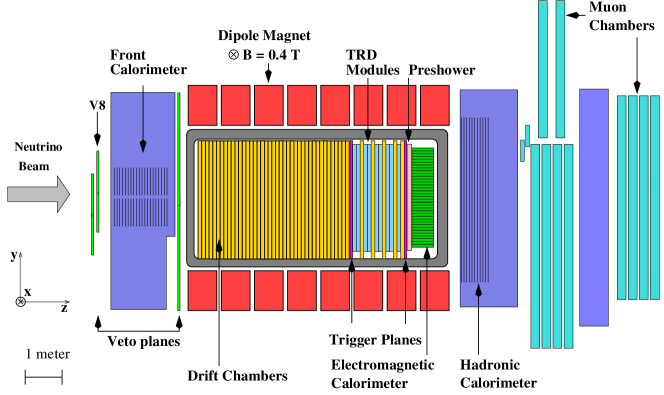
Figure 1: Side view of the NOMAD detector.

The large sample of neutrino interactions, about 1.5 millions, measured in NOMAD together with the good reconstruction quality of individual tracks, offer an excellent opportunity to search for $\Theta^{+}\to p+\mbox{$K^{0}_{S}$}$. The NOMAD detector  Altegoer:1998gv consisted of an active target of 44 drift chambers, with a total fiducial mass of 2.7 tons, located in a 0.4 Tesla dipole magnetic field, as shown in Fig. 1.

The drift chambers Anfreville:2001zi , made of low $Z$ material (mainly Carbon) served the double role of a nearly isoscalar target for neutrino interactions and of the tracking medium. The average density of the drift chamber volume was 0.1 $\mbox{g}/\mbox{cm}^{3}$. These chambers provided an overall efficiency for charged track reconstruction of better than 95% and a momentum resolution of approximately 3.5% in the momentum range of interest (less than 10 $\mbox{GeV}/\mbox{c}$). Reconstructed tracks were used to determine the event topology (the assignment of tracks to vertices), to reconstruct the vertex position and the track parameters at each vertex and, finally, to identify the vertex type (primary, secondary, $V^{0}$, etc.). A transition radiation detector Bassompierre1 ; Bassompierre2 placed at the end of the active target was used for particle identification. A lead-glass electromagnetic calorimeter Autiero:1996sp ; Autiero:1998ya located downstream of the tracking region provided an energy resolution of $3.2\%/\sqrt{E\mbox{[GeV]}}\oplus 1\%$ for electromagnetic showers and was crucial to measure the total energy flow in neutrino interactions. In addition, an iron absorber and a set of muon chambers located after the electromagnetic calorimeter were used for muon identification, providing a muon detection efficiency of 97% for momenta greater than 5 GeV/c.

Neutral strange particles were reconstructed and identified with high efficiency and purity using the $V^{0}$-like signature of their decays Astier:2000ax ; Astier . Proton identification needed further development for the search presented here using information from the drift chambers, transition radiation detector and electromagnetic calorimeter.

The NOMAD Monte Carlo simulation (MC) is based on LEPTO 6.1  Ingelman:1992ef and JETSET 7.4 Sjostrand generators for neutrino interactions, and on a GEANT GEANT based program for the detector response. The relevant JETSET parameters have been tuned in order to reproduce the yields of strange particles measured in $\nu_{\mu}$ CC interactions in NOMAD Astier . To define the parton content of the nucleon for the cross-section calculation we have used the parton density distributions parametrized in  Alekhin .

3 Event Selection

We have analysed neutrino–nucleon interactions of both charged (CC) and neutral current (NC) types. These events are selected with the requirements:

• The reconstructed primary vertex should be within a fiducial volume (FV) defined by $|x,y|<120$ cm, $5<z<395$ cm (see Fig. 1 for the definition of the NOMAD coordinate system)

• There should be at least two charged tracks originating from the primary vertex;

• The visible hadronic energy should be larger than 3 GeV.

The $\nu_{\mu}$ CC events are identified requiring in addition:

• The presence of an identified muon from the primary vertex.

The NC sample contains a contamination of about 30% from unidentified CC events. However, we do not apply further rejection against this background in order not to reduce the statistics. The event purity for the $\nu_{\mu}$ CC selection is $99.6\%$. The total sample amounts to about $1.5$ million neutrino events (see Table 1).

	CC	NC	CC+NC
$N_{obs}$	785232	393539	1178771
$N_{corr}$	1017664	481269	1498933

Table 1: Statistics of observed ($N_{obs}$) and efficiency corrected ($N_{corr}$) neutrino CC and NC events in the data.

3.1 $K^{0}_{S}$ Identification

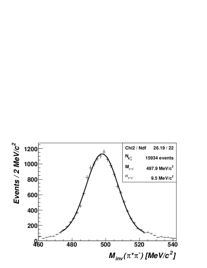
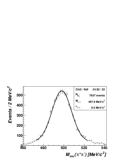
Figure 2: Reconstructed $K^{0}_{S}\to\pi^{+}\pi^{-}$ invariant mass distribution in the $\nu_{\mu}$ CC (left) and $\nu_{\mu}$ NC (right) data subsamples.

$K^{0}_{S}$ mesons are identified through their $V^{0}$-like decay
$K^{0}_{S}\to\pi^{+}\pi^{-}$ using a kinematic constrained fit Astier:2000ax ; Astier . With a purity of 97% we identify 15934 and 7657 $K^{0}_{S}$ mesons in the CC and NC samples respectively, thus yielding a total statistics of more than 23k $K^{0}_{S}$’s. The reconstructed $K^{0}_{S}\to\pi^{+}\pi^{-}$ invariant mass distribution in the $\nu_{\mu}$ CC (left) and $\nu_{\mu}$ NC (right) subsamples are shown in Fig. 2. The two distributions have the same $K^{0}_{S}$ mass mean value, 497.9 MeV$/c^{2}$, in agreement with the PDG value, and a width compatible with the expected experimental resolution of $\sim$9.5 MeV$/c^{2}$.

3.2 Proton Reconstruction

The identification of protons is the most difficult part of the present analysis. As the NOMAD experiment does not include a dedicated detector for proton identification, we developed a special procedure for this purpose. The main background in the proton selection is the $\pi^{+}$ contamination since pions are about 2.5 times more abundant than protons. However the $\pi^{+}$ contamination can be suppressed exploiting the differences in the behaviour of protons and pions propagating through the NOMAD detector. We use three sub-detectors which can provide substantial rejection factors against pions:

1. The Drift Chambers (DC). A low energy proton ranges out faster than a pion of the same momentum. Thus a correlation between the particle momentum and its path length can be used as a discriminator between protons and pions. The momentum interval of applicability of this method is below 600 MeV$/c$.

2. The Transition Radiation Detector (TRD). The energy deposition of protons and pions in the TRD is very different due to the larger proton ionization loss for momenta below 1 GeV$/c$, allowing a good pion–proton separation in this momentum interval. A modest discrimination is also possible for momenta above 3 GeV$/c$ because of relativistic rise effects.

3. The Electromagnetic Calorimeter (ECAL). The proton sample can be cleaned further by taking into account the different Cherenkov light emission of protons and pions of the same momentum.

As a preliminary quality selection for the candidate proton track we require :

• more than 7 hits on the DC track in order to have a reliable fit;

• the distance between the primary vertex and the first hit of the track to be smaller than 15 cm;

• the relative error on the track momentum to be smaller than 0.3;

• the coordinate of the last hit of the stopped particle to be within a fiducial volume (FV) defined as $|x|<120$ cm, $-110<y<100$ cm, $35<z<380$ cm, which is smaller than the FV used in the event selection in order to reduce edge effects;

• the particles reaching the TRD to cross at least 6 TRD planes (out of 9 in total) in order to allow for the TRD identification algorithm.

The initial sample of positively charged tracks is split into two subsamples: those that passed the quality criteria and those that did not. The identification cuts can be applied only to the positive tracks that passed the quality criteria. Charged particles were all assumed to be pions in the standard reconstruction program, resulting in a systematic underestimation of the reconstructed proton momentum ($p_{rec}$) at small momenta. The difference $\Delta p$ between the true and reconstructed proton momentum was studied with the help of the MC, and the following parametrization was found to describe the effect :

$$\Delta p=0.33\cdot e^{-\frac{3.5p_{rec}}{GeV/c}}\mbox{ GeV/c}.$$ (1)

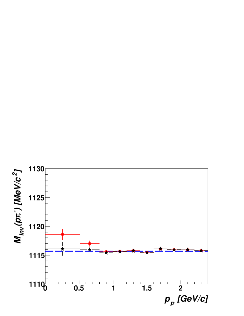
Figure 3: The mean value of the invariant mass of $p\pi^{-}$ pairs from identified $\Lambda$’s as a function of the reconstructed proton momentum with no momentum correction (full circles) and with momentum correction (stars).

The difference $\Delta p$ decreases with $p_{rec}$, becoming negligible at about 0.8 GeV/c. The reconstructed proton momentum was corrected accordingly. The effect of this proton correction was tested on a reconstructed sample of $\rm\Lambda$ hyperons identified by their displaced decay vertex. Fig. 3 displays the mean value of the invariant $p\pi^{-}$ mass as a function of the reconstructed proton momentum without and with the $\Delta p$ correction. There is an improvement in the reconstructed $\rm\Lambda$ mass when correcting the reconstructed proton momentum, especially at low momenta.

4 The background

Random $K^{0}_{S}$–proton pairs produce combinatorial background in the $K^{0}_{S}$p invariant mass ($M(\mbox{$K^{0}_{S}$}p)\equiv M$) distribution. Understanding the shape of this background is crucial in the search for a possible $\Theta^{+}$ signal. We studied this background in three different ways:

1. MC events contain no $\Theta^{+}$ and could be used, therefore,to study the background for this analysis. However, the small fraction of proton–$K^{0}_{S}$ pairs with an invariant mass in the interesting mass region would require a very large sample of MC events to reduce statistical fluctuations.

2. We combined protons and $\mbox{$K^{0}_{S}$}^{\prime}s$ from different events in the data, thus making fake pairs, paying special attention that the original data distributions of multiplicity, proton and kaon momenta, and their relative opening angle, were well reproduced in the final fake pair sample.

3. A polynomial fit to the $M$ distribution of the data themselves, excluding the $\Theta^{+}$ mass region, can also be used to describe the background for the $\Theta^{+}$ search.

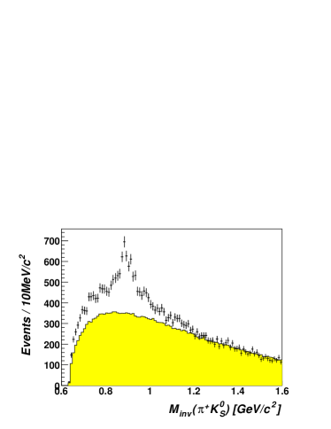
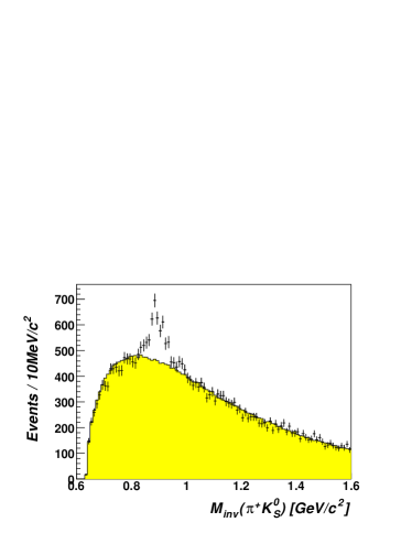
Figure 4: $\mbox{$K^{0}_{S}$}\pi^{+}$ invariant mass distribution in the data, superimposed with the background generated without hadronic jet rotation (left), and with hadronic jet rotation (right).

The fake pair technique is extensively used in the literature. However, it is necessary to ensure that the two independent events used in the mixing have similar hadronic jet momenta both in magnitude and direction. If two events with different jet momenta are mixed, then the fake pair technique systematically underestimates the background at small $M(\mbox{$K^{0}_{S}$}p)$ invariant masses. This is illustrated in the left panel of Fig. 4 which shows the $\mbox{$K^{0}_{S}$}\pi^{+}$ invariant mass distribution in the data, superimposed with the background generated without changing the hadronic jet directions. The background is normalized to the data at $M({\mbox{$K^{0}_{S}$}\pi^{+}})=1400$ MeV$/c^{2}$. The data show a clear $K^{*+}$ peak at $\sim 890$ MeV$/c^{2}$. However, the background under this peak is obviously underestimated. Therefore, in our procedure we first rotate each data event such that the hadronic jet momentum is aligned along the z-axis. We then select events respecting the original multiplicity of positive tracks and $K^{0}_{S}$ in the data and make random pairs. The right panel of Fig. 4 shows the same $\mbox{$K^{0}_{S}$}\pi^{+}$ invariant mass distribution in the data superimposed with the background generated according to our procedure. There is now a clear agreement with the data distribution, except for the $K^{*+}$ peak which the fake pair technique cannot reproduce.

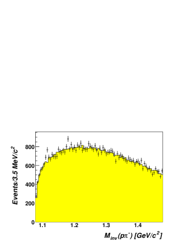
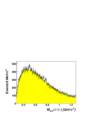
Figure 5: $p\pi^{-}$ (left) and $\pi^{+}\pi^{-}$ (right) invariant mass distribution (points with error bars) superimposed to the estimated background.

We have checked the background generation procedure on samples of $\mbox{$\rm\Lambda$}\to p\pi^{-}$ and $\mbox{$K^{0}_{S}$}\to\pi^{+}\pi^{-}$ events, using only tracks originating from the primary interaction vertex in order to artificially increase the background. Fig. 5 shows $p\pi^{-}$ and $\pi^{+}\pi^{-}$ invariant mass distributions superimposed with the predicted background estimated using our fake pair procedure. From these plots we conclude that our background generation procedure provides a realistic background estimate in these cases as well.

It is worth mentioning however that the fake pair tecnique does not take into account contributions from resonances which introduce correlations in $M$ different from those generated by making random pairs. $\Sigma(1660)-\Sigma(2250)$ decaying into proton and kaon and $K^{\star}\to K^{0}_{S}\pi$ decays with the pion taken as the proton might be important sources of distortion of the background shape. With help of MC we find a negligible contribution of $\Sigma(1660)-\Sigma(2250)$ resonances to $\mbox{$K^{0}_{S}$}p$ invariant mass distribution while $K^{\star}\to K^{0}_{S}\pi$ decays increase the background by 5-10% at small $M\sim 1500$ MeV$/c^{2}$. Therefore we renormalize the background distribution obtained by fake pair procedure by a ratio of two $\mbox{$K^{0}_{S}$}p$ distributions obtained with help of MC with and without $K^{\star}\to K^{0}_{S}\pi$ decays. Finally the obtained background distribution is normalized to the data distribution at $M>1650$ MeV$/c^{2}$. Fig. 6 shows the invariant mass distributions of combinations of a positively charged track, assumed to be a proton, and a $K^{0}_{S}$ for the data and for the fake pair background, without using proton identification and with “optimal“ proton identification. The “signal“ interval $1510<M<1550$ MeV$/c^{2}$ is excluded in the data. There is good agreement between the shapes of the data and background distributions. Polynomial fits of the data excluding the “signal“ interval $1510<M<1550$ MeV$/c^{2}$ is also shown as dashed curves. There is a reasonable agreement of the background shapes obtained by fake pair procedure and by a polynomial fit of the data.

5 $\Theta^{+}$ analysis tools

5.1 The proton identification strategy

The $\Theta^{+}$ signal is expected to appear as a narrow peak in the invariant mass distribution of $K^{0}_{S}$–proton pairs. $K^{0}_{S}$ are identified using their $V^{0}$-like signature (see Sec. 3.1). To separate protons from $\pi^{+}$, for each positively charged track we build likelihoods under the proton and $\pi^{+}$ hypothesis using the information from DC, TRD, and ECAL (see Sec. 3.2), and we take their ratios ${\cal L}_{DC}$, ${\cal L}_{TRD}$, ${\cal L}_{ECAL}$:

$${\cal L}_{DC}(p,L), L-\mbox{ track length}$$ (2)

$${\cal L}_{TRD}(p,\epsilon_{TRD}), \epsilon_{TRD}-\mbox{ energy release in TRD}$$

$${\cal L}_{ECAL}(p,\epsilon_{ECAL}), \epsilon_{ECAL}-\mbox{ energy release in ECAL}$$

$$p-\mbox{ track momentum. }$$

We optimize the cuts for the proton identification likelihood ratios maximizing the sensitivity to the expected $\Theta^{+}$ signal. These “optimal“ cuts are not necessarily those which maximize the purity of the proton sample.

The best approach for tuning the proton identification cuts would be to maximize the sensitivity using a detailed Monte Carlo for $\Theta^{+}$ production. However, given the poor knowledge on the properties of this particle, there is no available MC generator describing the production of exotic baryons. We create, therefore, “fake“ $\Theta^{+}$ states in the NOMAD event generator by using pairs of protons and $K^{0}_{S}$ with invariant mass close to the mass of $\Theta^{+}$ state. However, in this approach the momentum distribution of these “fake“ $\Theta^{+}$ states is determined by the momentum distribution of protons and $K^{0}_{S}$ from the primary vertex. This can result in wrong “optimal“ cuts if the true momentum distribution of $\Theta^{+}$ particles is very different. We try to avoid this problem by subdividing the original MC sample into several narrow bins of $x_{F}$ and optimizing the cuts for each $x_{F}$ interval independently. The $x_{F}$ variable is defined as the ratio of the longitudinal projection of the $\Theta^{+}$ momentum on the hadronic jet momentum to the hadronic jet energy in the hadronic center-of-mass frame. The variable $x_{F}$ is in the range $(-1,1)$ with negative (positive) values often called the target (current) fragmentation regions.

The procedure of tuning the proton identification cuts is then as follows:

• We build “fake“ $\Theta^{+}$ states by taking $K^{0}_{S}$–proton pairs with $1510<M<1550$ MeV$/c^{2}$. Assuming no $\Theta^{+}$ polarization, a flat distribution of $\cos\theta^{*}$, where $\theta^{*}$ is the angle between the proton momentum in the $\Theta^{+}$ rest frame and the $\Theta^{+}$ momentum in the laboratory. We reweight the $\cos\theta^{*}$ distribution so obtained to make it flat. This is our MC “signal“.

• Any other combination of a $K^{0}_{S}$ and a positive track not identified as a proton, but with an assigned proton mass, is taken as the MC background if its invariant mass M falls in the same mass interval.

• We split the “fake“ $\Theta^{+}$ states into several intervals of positive track momentum. We vary the cuts on ${\cal L}_{DC}$, ${\cal L}_{TRD}$, ${\cal L}_{ECAL}$ simultaneously in each interval and find those cuts which maximize the $signal/\sqrt{background}$ ratio.

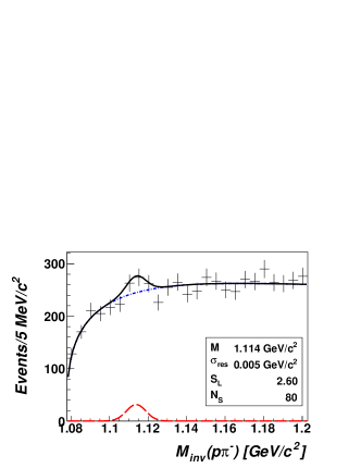
Figure 7: Invariant mass distributions of proton–$\pi^{-}$ pairs for $-0.6<x_{F}<-0.3$ interval. (Left, up) MC, no proton identification; (Right, up) MC, with “optimal“ proton identification; (Left, down) data, no proton identification; (Right, down) data, with “optimal“ proton identification. The curves represent the predicted background and the amount of $\rm\Lambda\to p\pi^{-}$ signal maximizing the $signal/\sqrt{background}$ ratio (see Sec. 5.1).

We check this procedure on a sample of $\rm\Lambda\to p\pi^{-}$ events. Fig. 7 displays the invariant mass distributions of proton–$\pi^{-}$ pairs in both MC and data without proton identification and with “optimal“ for the $\rm\Lambda\to p\pi^{-}$ observation proton identification, for $-0.6<x_{F}<-0.3$. With “optimal“ proton identification the significance of the $\rm\Lambda\to p\pi^{-}$ signal increases in both MC and data samples.

	$N({p\mbox{$K^{0}_{S}$}})$		purity (in %)
	all	“signal“	all	“signal“
no ID	53463	1856	23	16.4
“optimal“ ID	40561	1090	27.8	22.1

Table 2: Numbers of $p\mbox{$K^{0}_{S}$}$ pairs and purity of proton samples in the data for two subsets of events: without proton identification and with “optimal“ proton identification. These numbers are shown for all entries and for “signal“ region: $1510<M<1550$ MeV$/c^{2}$.

In Tab. 2 we show numbers of $p\mbox{$K^{0}_{S}$}$ pairs and purity of proton samples in the data for two subsets of events: without proton identification and with “optimal“ proton identification. These numbers are shown for all entries and for “signal“ region ($1510<M<1550$ MeV$/c^{2}$).

5.2 The $p\mbox{$K^{0}_{S}$}$ mass resolution

The expected mass resolution of the $p\mbox{$K^{0}_{S}$}$ pair is estimated as follows.

• For MC events we calculate the invariant masses of the generated and reconstructed $pK^{0}_{S}$ pairs, and we fit the distribution of the difference between the two values by a Gaussian whose width is taken as the mass resolution (method “A“).

• Using the measured momenta of the proton ($\vec{p}_{1}$) and of the $K^{0}_{S}$ ($\vec{p}_{2}$), the angle $\theta$ between $\vec{p}_{1}$ and $\vec{p}_{2}$, and the associated errors $\sigma(\vec{p}_{1})$ and $\sigma(\vec{p}_{2})$ we find (neglecting errors in $\cos\theta$):

  $$M^{2}_{inv}\ \sigma^{2}(M_{inv})= \left(\frac{E_{2}}{E_{1}}p_{1}-p_{2}\ cos\theta\right)^{2}\sigma^{2}(p_{1})+$$ (3)

  $$\left(\frac{E_{1}}{E_{2}}p_{2}-p_{1}\ cos\theta\right)^{2}\sigma^{2}(p_{2}).$$

  This method,“B“, can be applied to both MC and data events.

Fig. 8 displays the expected mass resolution of $p\mbox{$K^{0}_{S}$}$ pairs as a function of their reconstructed invariant mass, as obtained using method “A“ (MC only), or method “B“ (for both MC and data). The results agree well with each other and predict a resolution of about 8.8 MeV$/c^{2}$ at the $\Theta^{+}$ mass (1530 MeV$/c^{2}$).

5.3 The statistical analysis

An estimation of the signal significance in the data is performed as follows:

1. A possible difference in the proton $\cos\theta^{*}$ distribution for the signal and background is exploited to improve the signal sensitivity. We take all $K^{0}_{S}$–proton pairs with $1510<M<1550$ MeV$/c^{2}$, and we split them into 10 intervals with similar statistics: five mass intervals with $\cos\theta^{*}$ in the interval $[-1,-0.5)$, and another five mass intervals with $\cos\theta^{*}$ in the interval $[-0.5,1]$. The total mass interval ($1510<M<1550$ MeV$/c^{2}$) covers well the expected $\Theta^{+}$ mass. The mass bin width, 10 MeV$/c^{2}$, is comparable to the expected invariant mass resolution of $K^{0}_{S}$–proton pairs.

2. We compute two likelihoods:

   $$\ln L_{B} = \sum_{i=1,10}\left(-b_{i}+n_{i}\cdot\ln b_{i}\right)$$ (4)

   $$\ln L_{B+S} = \sum_{i=1,10}\left(-b_{i}-s_{i}+n_{i}\cdot\ln\left(b_{i}+s_{i}\right)\right)$$

   where $b_{i}$, $s_{i}$, $n_{i}$ are the number of predicted background and signal events, and observed data events in the $i$-th bin.

3. We compute the signal statistical significance as:

   $$S_{L}=\sqrt{2\left(\ln L_{B+S}-\ln L_{B}\right)}$$ (5)

4. We find the resonance mass position $M$ and Breit-Wigner width $\Gamma$ and the number of signal events $N_{s}$ which maximize $S_{L}$.

For the background we use the procedure decribed in Sec. 4. The signal is modeled by a Breit-Wigner distorted by a Gaussian resolution with $\sigma=8.8$ MeV$/c^{2}$. This algorithm was checked on several generated distributions containing a Breit-Wigner signal of width $\Gamma$ distorted by a Gaussian resolution of width $\sigma$ and superimposed on a fluctuating background. We considered three cases, $\sigma\ll\Gamma$, $\sigma=\Gamma$, $\sigma\gg\Gamma$, and found that in all cases the procedure of maximizing $S_{L}$ correctly determined the number of signal events and $\Gamma$ (with $\Gamma$ around zero for the case $\sigma\gg\Gamma$).

5.4 Opening the box

We split the data into five $x_{F}$ intervals:
$[-1,-0.6)$, $(-0.6,-0.3)$, $(-0.3,0)$, $(0,0.4)$, $(0.4,1]$. In each interval we optimize the proton identification cuts as described in Sec. 3.2, and estimate a possible signal in the region $1510<M<1550$ MeV$/c^{2}$ as described in Sec. 5.3. Figs. 9-13 display the results. From these plots we conclude that we observe no evidence for the $\Theta^{+}$ state in any $x_{F}$ interval. In Fig. 14 we display the invariant mass distributions of combinations of a positively charged track (assumed to be a proton) and a $K^{0}_{S}$ for the two cases of no proton identification and optimum proton identification, for $-1<x_{F}<1$. Table 3 summarizes the results and provides also the upper limits at 90% confidence level (CL) on the number of $\Theta^{+}$s candidates ($N_{s}^{up}$) and on the production rate $R^{up}$ for both cases. The calculation of the upper limits for the production rate include corrections for inefficiencies, including the lack of detection of $K^{0}_{L}$ mesons, and take into account the $K^{0}_{S}\to\pi^{+}\pi^{-}$ branching ratio. The results are presented for each bin of $x_{F}$, and also integrated over $x_{F}$.

$x_{F}$ interval	$[-1,-0.6)$	$(-0.6,-0.3)$	$(-0.3,0)$	$(0,0.4)$	$(0.4,1]$	all
no ID
$N_{s}$ (fit)	18	26	35	30	65	77
SL	1.96	1.49	1.01	1.18	2.61	1.82
$N_{s}^{up}$	41	61	88	81	101	161
$R^{up}$	3.84	2.18	1.74	1.37	0.83	4.36
optimal ID
$N_{s}$ (fit)	12	29	-26	-34	24	-33
SL	1.38	1.72	1.35	1.85	1.25	0.97
$N_{s}^{up}$	28	68	39	36	52	67
$R^{up}$	2.80	2.60	0.84	0.79	1.00	2.13

Table 3: Upper limits (90% CL) on the number of $\Theta^{+}$ candidates ($N_{s}^{up}$) and on the $\Theta^{+}$ production rate ($R^{up}$, in units of events per $10^{3}$ interactions) for the case of no proton identification and with optimal proton identification.

Fig. 16 displays the sensitivity and upper limits (90% CL) for the $\Theta^{+}$ production rate as a function of $x_{F}$. The upper limits are given as five curves, each corresponding to a fixed $\Theta^{+}$ mass, obtained by varying both the number of signal events and the $\Theta^{+}$ width to maximize $S_{L}$ as outlined in Sec. 5.3.

We also measure the $x_{F}$ distribution of a potential $\Theta^{+}$ state as follows. We build the $x_{F}$ distributions in two side-bands, $1460<M<1500$ MeV$/c^{2}$ and $1580<M<1600$ MeV$/c^{2}$. We then normalize the average of these two distributions to the expected number of background events in the “signal“ region ($1510<M<1550$ MeV$/c^{2}$), and subtract it from the $x_{F}$ distribution of the data in the “signal“ region. The result can be considered as the $x_{F}$ distribution of the signal, and could shed a light on the $\Theta^{+}$ production mechanism. Fig. 15 displays the result with no proton identification and with optimal proton identification. We observe no statistically significant accumulation of events at any $x_{F}$ value.

6 Conclusions

We have performed a blind search for the $\Theta^{+}$ exotic baryon in the $\Theta^{+}\to p+\mbox{$K^{0}_{S}$}$ decay mode in the NOMAD $\nu_{\mu}N$ data. We have built a robust background estimation procedure which has been tested against various known cases like $\rm\Lambda\to p\pi^{-}$, $K^{0}_{S}\to\pi^{+}\pi^{-}$ and $K^{\star}\to K^{0}_{S}\pi$. In all cases good agreement between data and estimated background has been found. Good agreement has also been found between the invariant mass ($M$) distribution of $K^{0}_{S}$–proton pairs in the data and the estimated background in the whole mass region excluding the $\Theta^{+}$ signal region. We have developed proton identification tools based on the discrimination power of three sub-detectors, and we have tuned the proton identification criteria by maximizing the sensitivity to the expected signal in five $x_{F}$ intervals independently. We have checked this approach for $\rm\Lambda\to p\pi^{-}$ and found that this procedure indeed maximizes the signal significance in both MC and data. Finally, we have “opened the box“, i.e. examined the $\Theta^{+}$ signal in the data and found good agreement between the data and the background for the whole $M$ region, including the “signal“ region, in each $x_{F}$ interval. We observe no evidence, therefore, for any $\Theta^{+}$ signal in the $\Theta^{+}\to p+\mbox{$K^{0}_{S}$}$ decay channel in the NOMAD $\nu_{\mu}N$ data. We give an upper limit at 90% CL on $\Theta^{+}$ production rate of $2.13\cdot 10^{-3}$ events per neutrino interaction at $M=1530$ MeV$/c^{2}$ after integrating over $x_{F}$.

It is interesting to compare this result with the recent analysis of old bubble chamber neutrino experiments which provide an estimation of the $\Theta^{+}$ production rate as large as $\sim 10^{-3}$  events per neutrino interactionBebc . As shown in Fig.16, for a large fraction of the $x_{F}$ range, except in the region $x_{F}\to-1$, such a value is excluded. Unfortunately, ref. Bebc does not provide information on the $x_{F}$ region in which a $\Theta^{+}$ signal was observed. Furthermore, in ref. Bebc we find no information that the background estimation procedure took into account the effects mentioned in Sec. 4, which can result in an underestimation of the background and thus in an overestimation of both the signal significance and the production rate.

Preliminary NOMAD results from searches for the exotic $\Theta^{+}$ baryon reported earlier  Camilleri:2005hc , quoting a hint for a signal with a statistical significance of 4.3 $\sigma$, suffered from an incorrect background estimation, which did not take into account the effects mentioned in Sec. 4. The results reported in  Camilleri:2005hc are obtained on a smaller sample of the NOMAD data. The positives of that sample were subjected for a cleaner proton identification which yielded an increase of the purity of the protons sample from 23% to 51.5% with about factor six lost of the statistics. The difference in shapes of $\mbox{$K^{0}_{S}$}p$ invariant mass distributions reported in  Camilleri:2005hc and in Figs. 6 is due to an additional requirement imposed in  Camilleri:2005hc on energy of protons to be larger than that of $K^{0}_{S}$.

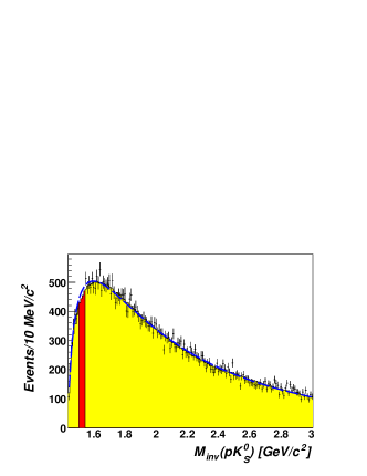
Figure 6: Invariant mass distribution of pairs of one positively charged track (assumed to be a proton) and a $K^{0}_{S}$ for the data (points with error bars) and for the fake pair background (shadowed area). (Left) Proton identification has not been used. (Right) “Optimal“ proton identification. Data in the “signal“ region ($1510<M<1550$ MeV$/c^{2}$) are not shown. Dashed curve is fit of the data by a polynomial excluding the “signal“ region.

Figure 8: Expected invariant mass resolution of proton–$K^{0}_{S}$ pairs as a function of the invariant mass for method “A“ (MC only), and for method “B“ (MC and data). See text for details.

Figure 9: Invariant mass distributions of pairs of a positively charged track (assumed to be a proton) and a $K^{0}_{S}$ in the data, for $-1<x_{F}<-0.6$. (Left) No proton identification; (Right) Optimized proton identification. The curves represent the predicted background and the amount of $\Theta^{+}$ signal maximizing $S_{L}$ (see Sec. 5.3).

Figure 10: Invariant mass distributions of pairs of a positively charged track (assumed to be a proton) and a $K^{0}_{S}$ in the data, for $-0.6<x_{F}<-0.3$. (Left) No proton identification; (Right) Optimized proton identification. The curves represent the predicted background and the amount of $\Theta^{+}$ signal maximizing $S_{L}$ (see Sec. 5.3).

Figure 11: Invariant mass distributions of pairs of a positively charged track (assumed to be a proton) and a $K^{0}_{S}$ in the data, for $-0.3<x_{F}<0$. (Left) No proton identification; (Right) Optimized proton identification. The curves represent the predicted background and the amount of $\Theta^{+}$ signal maximizing $S_{L}$ (see Sec. 5.3).

Figure 12: Invariant mass distributions of pairs of a positively charged track (assumed to be a proton) and a $K^{0}_{S}$ in the data, for $0<x_{F}<0.4$. (Left) No proton identification; (Right) Optimized proton identification. The curves represent the predicted background and the amount of $\Theta^{+}$ signal maximizing $S_{L}$ (see Sec. 5.3).

Figure 13: Invariant mass distributions of pairs of a positively charged track (assumed to be a proton) and a $K^{0}_{S}$ in the data, for $0.4<x_{F}<1$. (Left) No proton identification; (Right) Optimized proton identification. The curves represent the predicted background and the amount of $\Theta^{+}$ signal maximizing $S_{L}$ (see Sec. 5.3).

Figure 14: Invariant mass distributions of pairs of a positively charged track (assumed to be a proton) and a $K^{0}_{S}$ in the data, for $-1<x_{F}<1$. (Left) No proton identification; (Right) Optimized proton identification. The curves represent the predicted background and the amount of $\Theta^{+}$ signal maximizing $S_{L}$ (see Sec. 5.3).

Figure 15: $x_{F}$ distribution of a potential $\Theta^{+}$ signal in the data. (Left) No proton identification; (Right) Optimized proton identification.

Figure 16: Sensitivity and upper limits at 90% CL for $\Theta^{+}$ production rates as a function of $x_{F}$, for $\Theta^{+}$ masses of 1510, 1530, 1550 MeV$/c^{2}$.