Evidence for production of single top quarks and first direct measurement of $|V_{tb}|$

Abstract

The D0 Collaboration presents first evidence for the production of single top quarks at the Fermilab Tevatron $p\bar{p}$ collider. Using a 0.9 fb^-1 dataset, we apply a multivariate analysis to separate signal from background and measure $\sigma({\mbox{$p\bar{p}$}}{\mbox{ $\rightarrow$ }}tb+X,~{}tqb+X)=4.9\pm 1.4$ pb. The probability to measure a cross section at this value or higher in the absence of signal is $0.035\%$, corresponding to a 3.4 standard deviation significance. We use the cross section measurement to directly determine the CKM matrix element that describes the $Wtb$ coupling and find $0.68<|V_{tb}|\leq 1$ at $95\%$ C.L. within the standard model.

Top quarks were first observed in strong $t\bar{t}$ pair production at the Tevatron collider in 1995 top-obs-1995 . In the standard model (SM), $\sigma({\mbox{$p\bar{p}$}}{\mbox{ $\rightarrow$ }}{\mbox{$t\bar{t}$}}+X)=6.8^{+0.6}_{-0.5}$ pb ttbar-xsec-1 at $\sqrt{s}=1.96$ TeV for a top quark mass of 175 GeV. Top quarks are also expected to be produced singly via the electroweak processes singletop-theory ; singletop-yuan illustrated in Fig. 1. For brevity, we use the notation “$tb$” to represent the sum of $t\bar{b}$ and $\bar{t}b$, and “$tqb$” for the sum of $tq\bar{b}$ and $\bar{t}\bar{q}b$. The next-to-leading order (NLO) prediction for the s-channel single top quark cross section is $\sigma({\mbox{$p\bar{p}$}}{\mbox{ $\rightarrow$ }}tb+X)=0.88\pm 0.11$ pb, and for the t-channel process, the prediction is $\sigma({\mbox{$p\bar{p}$}}{\mbox{ $\rightarrow$ }}tqb+X)=1.98\pm 0.25$ pb singletop-xsec-sullivan ; singletop-xsec-kidonakis .

Figure 1: Representative Feynman diagrams for (a) s-channel single top quark production and (b) t-channel production.

Single top quark events can be used to study the $Wtb$ coupling singletop-wtb-heinson , and to measure the magnitude of the element $|V_{tb}|$ of the quark mixing matrix, (the Cabibbo-Kobayashi-Maskawa (CKM) matrix ckm-matrix ), without assuming only three generations of quarks singletop-vtb-jikia . The quark mixing matrix must be unitary, which for three families implies $|V_{tb}|\simeq 1$ pdb-vtb . A smaller measured value would indicate the presence of a fourth quark family to make up the difference. Single top quark production can also be used to measure the top quark partial decay width $\Gamma(t{\rightarrow}Wb)$ singletop-width-yuan and hence the top quark lifetime.

The D0 collaboration has previously published limits limits-d0 on single top quark production. The best $95\%$ C.L. upper limits are $\sigma({\mbox{$p\bar{p}$}}{\mbox{ $\rightarrow$ }}tb+X)<6.4$ pb and $\sigma({\mbox{$p\bar{p}$}}{\mbox{ $\rightarrow$ }}tqb+X)<5.0$ pb. The CDF collaboration has also published limits on the cross sections limits-cdf .

This Letter describes a search for single top quark production using 0.9 fb^-1 of data produced at a center-of-mass energy of 1.96 TeV. The data were collected from 2002 to 2005 using the D0 detector d0-detector with triggers that required a jet and an electron or a muon. The search focuses on the final state consisting of one high transverse momentum ($p_{T}$) isolated lepton and missing transverse energy ($\not\!\!E_{T}$), together with a $b$-quark jet from the decay of the top quark ($t{\rightarrow}Wb{\rightarrow}\ell\nu b$). There is an additional $b$ quark in s-channel production, and an additional light quark and $b$ quark in t-channel production. The second $b$ quark in the t-channel is rarely reconstructed since it is produced in the forward direction with low transverse momentum. The main backgrounds are: $W$ bosons produced in association with jets; top quark pairs decaying into the lepton+jets and dilepton final states, when a jet or a lepton is not reconstructed; and multijet production, where a jet is misreconstructed as an electron, or a heavy-flavor quark decays to a muon that passes the isolation criteria.

We model the signal using the singletop NLO Monte Carlo (MC) event generator singletop-mcgen . The event kinematics for both s-channel and t-channel reproduce distributions found in NLO calculations singletop-xsec-sullivan . The decays of the top quark and resulting $W$ boson, with finite widths, are modeled in the singletop generator to preserve particle spin information. Pythia pythia is used to model the hadronization of the generated partons. For the $tb$ search, we assume SM $tqb$ as part of the background, and vice versa. For the $tb$+$tqb$ search, we assume the SM ratio between the $tb$ and $tqb$ cross sections.

We simulate the $t\bar{t}$ and $W$+jets backgrounds using the alpgen leading-order MC event generator alpgen and pythia to model the hadronization. A parton-jet matching algorithm jet-matching is used to ensure there is no double-counting of the final states. The $t\bar{t}$ background is normalized to the integrated luminosity times the predicted $t\bar{t}$ cross section ttbar-xsec-1 . The multijet background is modeled using data that contain nonisolated leptons but which otherwise resemble the lepton+jets dataset. The $W$+jets background, combined with the multijet background, is normalized to the lepton+jets dataset separately for each analysis channel (defined by lepton flavor and jet multiplicity) before $b$-jet tagging (described later). In the $W$+jets background simulation, we scale the $Wb\bar{b}$ and $Wc\bar{c}$ components by a factor of $1.50\pm 0.45$ to better represent higher-order effects wbb-wbj-nlo . This factor is determined by scaling the numbers of events in an admixture of light- and heavy-flavor $W$+jets MC events to data that have no $b$ tags but which otherwise pass all selection cuts. The uncertainty assigned to this factor covers the expected dependence on kinematics and the assumption that the factor is the same for $Wb\bar{b}$ and $Wc\bar{c}$.

We pass the MC events through a geant-based simulation geant of the D0 detector. To correct differences between the simulation and data, we apply weights to the simulated events to model the effects of the triggers, lepton identification and isolation requirements, and the energy scale of the jets. The $b$-tagging algorithm btagging-scanlon is modeled by applying weights that account for the probability for each jet to be tagged as a function of jet flavor, $p_{T}$, and pseudorapidity $\eta$.

We choose events with two, three, or four jets, reconstructed using a cone algorithm cone-algorithm with radius $\mathcal{R}=\sqrt{(\Delta y)^{2}+(\Delta\phi)^{2}}=0.5$ (where $y$ is rapidity and $\phi$ is azimuthal angle) to cluster energy deposits in the calorimeter. The leading jet has $p_{T}>25$ GeV and $|\eta|<2.5$, the second leading jet has $p_{T}>20$ GeV and $|\eta|<3.4$, and subsequent jets have $p_{T}>15$ GeV and $|\eta|<3.4$. Events are required to have $15<\mbox{$\not\!\!E_{T}$}<200$ GeV and exactly one isolated electron with $p_{T}>15$ GeV and $|\eta|<1.1$ or one isolated muon with $p_{T}>18$ GeV and $|\eta|<2.0$. Misreconstructed events are rejected by requiring that the direction of the $\not\!\!E_{T}$ is not aligned or anti-aligned in azimuth with the lepton or a jet. To enhance the signal content of the selection, one or two of the jets are required to be identified as originating from long-lived $b$ hadrons by a neural network $b$-jet tagging algorithm. The variables used to identify such jets rely on the presence and characteristics of a secondary vertex and tracks with high impact parameters inside the jet. For a $0.5\%$ light-jet $b$-tag efficiency (the average mistag probability), we obtain a $50\%$ average tag rate in data for $b$ jets with $|\eta|<2.4$.

We select 1,398 $b$-tagged lepton+jets data events, which we expect to contain $62\pm 13$ single top quark events. To increase the search sensitivity, we divide these events into twelve independent analysis channels based on the lepton flavor ($e$ or $\mu$), jet multiplicity (2, 3, or 4), and number of identified $b$ jets (1 or 2). We do this because the signal acceptance and signal-to-background ratio differ significantly from channel to channel. Event yields are given in Table 1, shown separated only by jet multiplicity for simplicity. The acceptances for single top quark signal as percentages of the total production cross sections are $(3.2\pm 0.4)\%$ for $tb$ and $(2.1\pm 0.3)\%$ for $tqb$.

The dominant contributions to the uncertainties on the backgrounds come from: normalization of the $t\bar{t}$ background (18% of the $t\bar{t}$ component), which includes a term to account for the top quark mass uncertainty; normalization of the $W$+jets and multijet backgrounds to data (17–27%), which includes the uncertainty on the heavy-flavor fraction of the model; the jet energy scale corrections (1–20%); and the $b$-tagging probabilities (12–17% for double-tagged events). The uncertainty on the integrated luminosity is 6%; all other sources contribute at the few percent level. The uncertainties from the jet energy scale corrections and the $b$-tagging probabilities affect both the shape and normalization of the simulated distributions. Having selected the data samples, we check that the background model reproduces the data in a multitude of variables (e.g., transverse momenta, pseudorapidities, azimuthal angles, masses) for each analysis channel and find agreement within uncertainties.

Table 1: Numbers of expected and observed events in 0.9 fb^-1 for $e$ and $\mu$, 1 $b$ tag and 2 $b$ tag channels combined. The total background uncertainties are smaller than the component uncertainties added in quadrature because of anticorrelation between the $W$+jets and multijet backgrounds resulting from the background normalization procedure.

Source	2 jets		3 jets		4 jets
$tb$	16$\pm$	3	8$\pm$	2	2$\pm$	1
$tqb$	20$\pm$	4	12$\pm$	3	4$\pm$	1
${\mbox{$t\bar{t}$}}{\rightarrow}\ell\ell$	39$\pm$	9	32$\pm$	7	11$\pm$	3
${\mbox{$t\bar{t}$}}{\rightarrow}\ell$+jets	20$\pm$	5	103$\pm$	25	143$\pm$	33
$Wb\bar{b}$	261$\pm$	55	120$\pm$	24	35$\pm$	7
$Wc\bar{c}$	151$\pm$	31	85$\pm$	17	23$\pm$	5
$Wjj$	119$\pm$	25	43$\pm$	9	12$\pm$	2
Multijets	95$\pm$	19	77$\pm$	15	29$\pm$	6
Total background	686$\pm$	41	460$\pm$	39	253$\pm$	38
Data	697		455		246

Since we expect single top quark events to constitute only a small fraction of the selected event samples, and since the background uncertainty is larger than the expected signal, a counting experiment will not have sufficient sensitivity to verify their presence. We proceed instead to calculate multivariate discriminants that separate the signal from background and thus enhance the probability to observe single top quarks. We use decision trees decision-trees to create these discriminants. A decision tree is a machine-learning technique that applies cuts iteratively to classify events. The discrimination power is further improved by averaging over many decision trees constructed using the adaptive boosting algorithm AdaBoost adaboost . We refer to this average as a boosted decision tree.

We identify 49 variables from an analysis of the signal and background Feynman diagrams singletop-vars-dudko-boos , studies of single top quark production at NLO singletop-vars-cao , and from other analyses singletop-yuan ; singletop-vars-mahlon-parke . The variables may be classified into three categories: individual object kinematics, global event kinematics, and variables based on angular correlations. Those with the most discrimination power include the invariant mass of all the jets in the event, the invariant mass of the reconstructed $W$ boson and the highest-$p_{T}$ $b$-tagged jet, the angle between the highest-$p_{T}$ $b$-tagged jet and the lepton in the rest frame of the reconstructed top quark, and the lepton charge times the pseudorapidity of the untagged jet. We find that reducing the number of variables always reduces the sensitivity of the analysis.

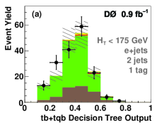
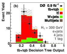
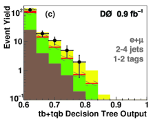
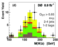
We use a boosted decision tree (DT) in each of the twelve analysis channels for three searches: $tb$+$tqb$, $tqb$, and $tb$. These 36 DTs are trained to separate one of the signals from the sum of the $t\bar{t}$ and $W$+jets backgrounds. One-third of the MC signal and background events is used for training; the remaining two-thirds are used to determine the acceptances in an unbiased manner. A boosted decision tree produces a quasi-continuous output distribution $O_{\rm DT}$ ranging from zero to one, with background peaking closer to zero and signal peaking closer to one. Figures 2(a) and 2(b) show the DT output distributions for two background-dominated data samples to demonstrate the agreement between background model and data. Figure 2(c) shows the high end of the sum of the 12 $tb$+$tqb$ DT outputs to illustrate where the signal is expected, and Fig. 2(d) shows the invariant mass of the reconstructed $W$ boson with the highest-$p_{T}$ $b$-tagged jet (where the neutrino longitudinal momentum has been chosen to be the smaller absolute value of the two possible solutions to the mass equation), for events in a signal-enhanced region with $O_{\rm DT}>0.65$. The background peaks near the top quark mass because the DTs select events similar to single top quark events.

Figure 2: Boosted decision tree output distributions for (a) a $W$+jets-dominated control sample, (b) a $t\bar{t}$-dominated control sample, and (c) the high-discriminant region of the sum of all 12 $tb$+$tqb$ DTs. For (a) and (b), $H_{T}=E_{T}^{\ell}+{\mbox{$\not\!\!E_{T}$}}+\sum E_{T}^{\rm alljets}$. Plot (d) shows the invariant mass of the reconstructed $W$ boson and highest-$p_{T}$ $b$-tagged jet for events with $O_{\rm DT}>0.65$. The hatched bands show the $\pm 1$ standard deviation uncertainty on the background. The expected signal is shown using the measured cross section.

We apply a Bayesian approach bayes-limits to measure the single top quark production cross section. We form a binned likelihood as a product over all bins and channels (lepton flavor, jet multiplicity, and tag multiplicity) of the decision tree discriminant, separately for the $tb$+$tqb$, $tqb$, and $tb$ analyses. We assume a Poisson distribution for the observed counts and flat nonnegative prior probabilities for the signal cross sections. Systematic uncertainties and their correlations are taken into account by integrating over the signal acceptances, background yields, and integrated luminosity with Gaussian priors for each systematic uncertainty. The final posterior probability density is computed as a function of the production cross section. For each analysis, we measure the cross section using the position of the posterior density peak and we take the $68\%$ asymmetric interval about the peak as the uncertainty on the measurement.

We test the validity of the cross section measurement procedure using six ensembles of pseudo-datasets selected from the full set of $tb$+$tqb$ signal and background events weighted to represent their expected proportions. A Poisson distribution with a mean equal to the total number of selected events is randomly sampled to determine the number of events in each pseudo-dataset. Each ensemble has a different assumed $tb$+$tqb$ cross section between 2 pb and 8 pb. No significant bias is seen in the mean of the measured cross sections for these ensembles.

The expected SM and measured posterior probability densities for $tb$+$tqb$ are shown in Fig. 3. We use the measured posterior density distribution for $tb$+$tqb$ as shown in Fig. 3 and similar distributions for $tqb$ and $tb$ to make the following measurements: $\sigma({\mbox{$p\bar{p}$}}{\mbox{ $\rightarrow$ }}tb+X,~{}tqb+X)=4.9\pm 1.4$ pb, $\sigma({\mbox{$p\bar{p}$}}{\mbox{ $\rightarrow$ }}tqb+X)=4.2^{+1.8}_{-1.4}$ pb, and $\sigma({\mbox{$p\bar{p}$}}{\mbox{ $\rightarrow$ }}tb+X)=1.0\pm 0.9$ pb. These results are consistent with the SM expectations. The uncertainties include statistical and systematic components combined. The data statistics contribute 1.2 pb to the total 1.4 pb uncertainty on the $tb$+$tqb$ cross section.

Figure 3: Expected SM and measured Bayesian posterior probability densities for the $tb$+$tqb$ cross section. The shaded regions indicate one standard deviation above and below the peak positions.

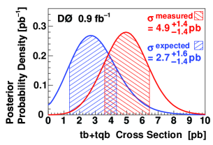
We assess how strongly this analysis rules out (or is expected to rule out) the background-only hypothesis by measuring the probability for the background to fluctuate up to give the measured (or SM) value of the $tb$+$tqb$ cross section or greater. From an ensemble of over 68,000 background-only pseudo-datasets, with all systematic uncertainties included, we find that the background fluctuates up to give the SM cross section of 2.9 pb or greater $1.9\%$ of the time, corresponding to an expected significance of 2.1 standard deviations (SD) for a Gaussian distribution. The probability that the background fluctuates up to produce the measured cross section of 4.9 pb or greater is $0.035\%$, corresponding to a significance for our result of 3.4 SD. Using a second ensemble of pseudo-datasets which includes a SM $tb$+$tqb$ signal with 2.9 pb cross section, with all systematic uncertainties included, we find the probability to measure a cross section of at least 4.9 pb to be $11\%$.

We apply two alternative methods to calculate $tb$+$tqb$ discriminants. The first technique calculates the probability for each event to be signal or background based on the leading-order matrix element description of each process for two-jet and three-jet events matrix-elements . It takes as input the four-momenta of the reconstructed objects and incorporates the $b$-tagging information for each event. This is a powerful method to extract the small signal because it encodes the kinematic information of the signal and background processes at the parton level. The probability that the background fluctuates up to give the SM cross section or greater in the matrix element analysis is $3.7\%$ (1.8 SD). We measure $\sigma({\mbox{$p\bar{p}$}}{\mbox{ $\rightarrow$ }}tb+X,~{}tqb+X)=4.6^{+1.8}_{-1.5}$ pb. The probability for the background to fluctuate up to give a cross section of at least 4.6 pb is $0.21\%$ (2.9 SD). The second alternative method uses Bayesian neural networks bayesianNNs to separate $tb$+$tqb$ signal from background. We train the networks separately for each analysis channel on a sample of signal events and on an equal-sized sample of background events containing the background components in their expected proportions, using 24 input variables (a subset of the 49 used in the boosted decision tree analysis). Large numbers of networks are averaged, resulting in better separation than can be achieved with a single network. The probability that the background fluctuates up to give the SM cross section or greater in the Bayesian neural network analysis is $9.7\%$ (1.3 SD). We measure $\sigma({\mbox{$p\bar{p}$}}{\mbox{ $\rightarrow$ }}tb+X,~{}tqb+X)=5.0\pm 1.9$ pb. The probability for the background to fluctuate up to give a cross section of at least 5.0 pb is $0.89\%$ (2.4 SD).

The three analyses are correlated since they use the same signal and background models and data, with almost the same systematic uncertainties. We take the decision tree measurement as our main result because this method has the lowest a priori probability for the background to have fluctuated up to give the SM cross section or greater. That is, we expect the decision tree analysis to rule out the background-only hypothesis with greatest significance.

We use the decision tree measurement of the $tb$+$tqb$ cross section to derive a first direct measurement of the strength of the $V$$-$$A$ coupling $|V_{tb}f_{1}^{L}|$ in the $Wtb$ vertex, where $f_{1}^{L}$ is an arbitrary left-handed form factor vtb-theory . We measure $|V_{tb}f_{1}^{L}|=1.3\pm 0.2$. This measurement assumes $|V_{td}|^{2}+|V_{ts}|^{2}\ll|V_{tb}|^{2}$ and a pure $V$$-$$A$ and CP-conserving $Wtb$ interaction. Assuming in addition that $f_{1}^{L}=1$ and using a flat prior for $|V_{tb}|^{2}$ from 0 to 1, we obtain $0.68<|V_{tb}|\leq 1$ at $95\%$ C.L. These measurements make no assumptions about the number of quark families or CKM matrix unitarity.

To summarize, we have performed a search for single top quark production using 0.9 fb^-1 of data collected by the D0 experiment at the Tevatron collider. We find an excess of events over the background prediction in the high discriminant output region and interpret it as evidence for single top quark production. The excess has a significance of 3.4 standard deviations. We use the boosted decision tree discriminant output distributions to make the first measurement of the single top quark cross section: $\sigma({\mbox{$p\bar{p}$}}{\mbox{ $\rightarrow$ }}tb+X,~{}tqb+X)=4.9\pm 1.4$ pb. We use this cross section measurement to make the first direct measurement of the CKM matrix element $|V_{tb}|$ without assuming CKM matrix unitarity, and find $0.68<|V_{tb}|\leq 1$ at $95\%$ C.L.

We thank the staffs at Fermilab and collaborating institutions, and acknowledge support from the DOE and NSF (USA); CEA and CNRS/IN2P3 (France); FASI, Rosatom and RFBR (Russia); CAPES, CNPq, FAPERJ, FAPESP and FUNDUNESP (Brazil); DAE and DST (India); Colciencias (Colombia); CONACyT (Mexico); KRF and KOSEF (Korea); CONICET and UBACyT (Argentina); FOM (The Netherlands); PPARC (United Kingdom); MSMT (Czech Republic); CRC Program, CFI, NSERC and WestGrid Project (Canada); BMBF and DFG (Germany); SFI (Ireland); The Swedish Research Council (Sweden); The Radcliffe Institute Fellowship program; Research Corporation; Alexander von Humboldt Foundation; and the Marie Curie Program.