Study of $\bar{B^{0}}\to{D}^{0}\pi^{+}\pi^{-}$ decays

Abstract

We report the results of a study of neutral $B$ meson decays to the $D^{0}\pi^{+}\pi^{-}$ final state, where the $D^{0}$ is fully reconstructed. The results are obtained from an event sample containing 388 million $B\bar{B}$-meson pairs collected in the Belle experiment at the KEKB $e^{+}e^{-}$ collider. The total branching fraction of the three-body decay ${\cal B}(\bar{B}^{0}\to D^{0}\pi^{+}\pi^{-})=(8.4\pm 0.4{\rm(stat.)}\pm 0.8{\rm(syst.)})\times 10^{-4}$ has been measured. The intermediate resonant structure of these three-body decays has been studied. From a Dalitz plot analysis we have obtained the product of the branching fractions for $D^{*+}_{2}$ and $D^{*+}_{0}$ production: ${\cal B}(\bar{B}^{0}\to D^{*+}_{2}\pi^{-})\times{\cal B}(D_{2}^{*+}\to D^{0}\pi^{+})=(2.15\pm 0.17{\rm(stat.)}\pm 0.29{\rm(syst.)}\pm 0.12{\rm(mod.)})\times 10^{-4},$ and ${\cal B}(\bar{B}^{0}\to D^{*+}_{0}\pi^{-})\times{\cal B}(D_{0}^{*+}\to D^{0}\pi^{+})=(0.60\pm 0.13{\rm(stat.)}\pm 0.15{\rm(syst.)}\pm 0.22{\rm(mod.)})\times 10^{-4}.$ This is the first observation of the $\bar{B}^{0}\to D^{*+}_{0}\pi^{-}$ decay. The $\bar{B^{0}}\to D^{0}\rho^{0}$ and $D^{0}f_{2}$ branching fractions are measured to be: ${\cal B}(\bar{B}^{0}\to D^{0}\rho^{0})=(3.19\pm 0.20{\rm(stat.)}\pm{0.24}{\rm(syst.)}\pm 0.38{\rm(mod.)})\times 10^{-4},$ and ${\cal B}(\bar{B}^{0}\to D^{0}f_{2})=(1.20\pm 0.18{\rm(stat.)}\pm 0.21{\rm(syst.)}\pm 0.32{\rm(mod.)})\times 10^{-4}.$

I Introduction

The decay $\bar{B}^{0}\to{D}^{0}\pi^{+}\pi^{-}$ includes intermediate states $D^{**^{+}}\pi^{-}$, where $D^{**}$’s are $P$-wave excitations of states containing one charmed and one light ($q=u,d$) quark that decay to the $D^{0}\pi^{+}$ final state. Figure 1 shows the spectrum and the allowed transitions of $c\bar{q}$-meson states. In the heavy-quark limit, the $c$-quark spin ${\vec{s}}_{c}$ decouples from the other degrees of freedom, and the total angular momentum of the light quark ${\vec{j}}_{q}=\vec{L}+{\vec{s}}_{q}$ is a good quantum number. Four $P$-wave states with the quantum numbers $0^{+}(j_{q}=1/2),~{}1^{+}(j_{q}=1/2),~{}1^{+}(j_{q}=3/2)$ and $2^{+}(j_{q}=3/2)$ are expected; these are usually labeled as $D^{*}_{0},~{}D^{\prime}_{1},~{}D_{1}$ and $D^{*}_{2}$, respectively.

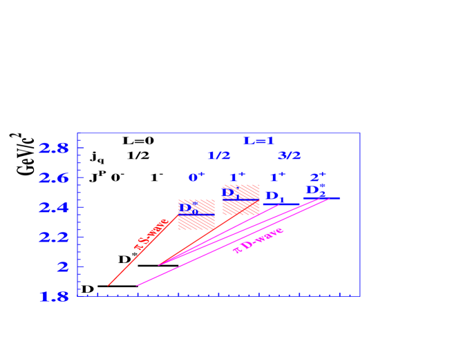
Figure 1: Spectrum of $c\bar{q}$-meson excitations. The lines indicate possible one-pion transitions. The $D^{*}_{0},~{}D^{\prime}_{1}$ mesons are broad which is indicated by shaded areas.

The two $j_{q}=3/2$ states have narrow widths of about 20-40 MeV and are well established AR1 ; AR2 ; AR3 ; e691 ; CL15 ; e687 ; CL2 ; dobs ; DELPHI ; DELPHI1 ; ALEPH . The measured masses agree with model predictions isgur ; rosner ; godfrey ; falk . The remaining $j_{q}=1/2$ states are expected to be broad and decay via $S$-waves. The $B\to D\pi\pi$ decay process provides a way to study $D^{**}$ production. Angular analysis of the decay products can be used to determine $D^{**}$ meson quantum numbers. These results also provide a test of Heavy Quark Effective Theory (HQET) and QCD sum rules QCDSR1 ; QCDSR .

A study of neutral $D^{**0}$ production in charged $B$-decays has been recently reported by Belle mybelle , where four $D^{**}$ states are observed and the production rates of the broad ($j=1/2$) states are found to be of the same order-of-magnitude as those for the narrow ($j=3/2$) states. This paper describes an analysis of the $B^{0}\to\bar{D}^{0}\pi^{+}\pi^{-}$ decay that is performed in a manner similar to that of the previous Belle analysis of the $\bar{B}^{0}\to D^{**+}\pi^{-}$ decay hhh . The results presented here supersede those of Ref. hhh .

The neutral $B$ decay to $D^{**}\pi$ is described by the tree diagram only as shown in Fig. 2(a) while for the charged $B$ decay to $D^{**}\pi$, the amplitude receives contributions from both tree and color-suppressed diagrams as shown in Fig. 2(b,c).

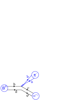
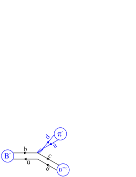
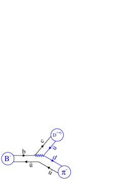
a)	b)	c)

Figure 2: Quark-line diagrams for neutral (a) and charged (b and c) $B$ decays.

$D^{**}$ tree-diagram production amplitudes are described by the Isgur-Wise functions $\tau_{1/2}$ and $\tau_{3/2}$. According to the QCD sum rule QCDSR1 ; QCDSR , $\tau_{1/2}\ll\tau_{3/2}$ and one would expect suppression of decays to the broad state. The observation that the production rates of the broad ($j=1/2$)-states are comparable with those of the narrow ($j=3/2$)-states indicates either a large contribution of the color-suppressed diagram or the violation of the sum rule above. Measurement of the decay rates of the neutral $B$ allows one to test the contribution of the tree-diagram only and also test the QCD sum rule.

In this analysis, the final state contains two pions of opposite sign, and these can originate from resonant states such as the $\rho^{0},~{}f_{0},~{}f_{2}$, etc. While the possible presence of $\pi\pi$ resonant structures complicates the analysis, it can also provide valuable information about the mechanism of these decays.

II The Belle detector

The Belle detector Belle is a large-solid-angle magnetic spectrometer that consists of a silicon vertex detector (SVD), a 50-layer central drift chamber (CDC) for charged particle tracking and specific ionization measurement ($dE/dx$), an array of aerogel threshold Čerenkov counters (ACC), time-of-flight scintillation counters (TOF), and an array of 8736 CsI(Tl) crystals for electromagnetic calorimetry (ECL) located inside a superconducting solenoid coil that provides a 1.5 T magnetic field. An iron flux return located outside the coil is instrumented to detect $K_{L}^{0}$ mesons and identify muons (KLM). We use a GEANT-based Monte Carlo (MC) simulation to model the response of the detector and determine its acceptance sim .

Separation of kaons and pions is accomplished by combining the responses of the ACC and the TOF with $dE/dx$ measurements in the CDC to form a likelihood $\cal{L}$($h$) where $h=(\pi)$ or $(K)$. Charged particles are identified as pions or kaons using the likelihood ratio (${\mathcal{R}}$):

$${\rm{\mathcal{R}}}(K)=\frac{{\cal{L}}(K)}{{\cal{L}}(K)+{\cal{L}}(\pi)};~{}~{}{\rm{\mathcal{R}}}(\pi)=\frac{{\cal{L}}(\pi)}{{\cal{L}}(K)+{\cal{L}}(\pi)}=1-{\rm{\mathcal{R}}}(K).$$

A more detailed description of the Belle particle identification can be found in Ref. PID .

III Event selection

A data sample of 357 fb^-1 (388 million $B\bar{B}$ events) collected at the $\Upsilon(4S)$ resonance is used in this analysis. Candidate $\bar{B}^{0}\to D^{0}\pi^{+}\pi^{-}$ events are selected, where the $D^{0}$ mesons decay via the $D^{0}\to K^{-}\pi^{+}$ mode. The signal-to-noise ratios for other $D^{0}$ decay modes are found to be significantly lower and, therefore, are not used. (The inclusion of charge conjugate states is implied by default throughout this paper.)

Charged tracks are selected with requirements based on the average hit residuals and impact parameters relative to the interaction point. We require that the polar angle of each track be in the angular range of $17^{\circ}-150^{\circ}$ and that the track transverse momentum be greater than 50 MeV/$c$ for kaons and greater than 25 MeV/$c$ for pions.

Charged kaon candidates are identified by the requirement ${\rm{\mathcal{R}}}(K)>0.6$, which has an efficiency of $90\%$ and a pion misidentification probability of approximately $10\%$. For pion candidates we require ${\rm{\mathcal{R}}}(\pi)>0.2$. Kaon and pion candidates are rejected if the track is positively identified as an electron.

Candidate $D^{0}$ mesons are $K^{-}\pi^{+}$ combinations with an invariant mass within $\pm$12 MeV/c² of the nominal $D^{0}$ mass, which corresponds to $\sim$2.5 $\sigma_{K\pi}$. We reject $D^{0}$ candidates that, when combined with any $\pi^{0}$ in the event, has a value of $M_{D\pi^{0}}-M_{D^{0}}$ that is within $\pm 2.5~{}{\rm MeV}/c^{2}$ of the nominal $D^{*0}$-$D^{0}$ mass difference.

$B$ meson candidates are identified by their center-of-mass (c.m.) energy difference $\Delta E=(\sum_{i}E_{i})-E_{\rm b}$, and the beam-constrained mass $M_{\rm bc}=\sqrt{E^{2}_{\rm b}-(\sum_{i}\vec{p}_{i})^{2}}$, where $E_{\rm b}=\sqrt{s}/2$ is the beam energy in the $\Upsilon(4S)$ c.m. frame, and $\vec{p}_{i}$ and $E_{i}$ are the c.m. three-momenta and energies, respectively of the $B$ meson candidate decay products. We select events satisfying $M_{\rm bc}>5.25$ GeV/$c^{2}$ and $|\Delta E|<0.10$ GeV.

To suppress the large continuum background ($e^{+}e^{-}\to q\bar{q}$, where $q=u,d,s,c$), topological variables are used. Since the produced $B$ mesons are almost at rest in the c.m. frame, the signal event shapes tend to be isotropic while continuum $q\bar{q}$ events tend to have a two-jet structure. We use the angle between the thrust axis of the $B$ candidate and that of the rest of the event ($\Theta_{\rm thrust}$) to discriminate between these two cases. The distribution of $|\cos\Theta_{\rm thrust}|$ is strongly peaked near $|\cos\Theta_{\rm thrust}|=1$ for $q\bar{q}$ events and is nearly flat for $\Upsilon(4S)\to B\bar{B}$ events. We require $|\cos\Theta_{\rm thrust}|<0.8$, which eliminates about 83$\%$ of the continuum background while retaining about 80$\%$ of signal events.

There are events for which two or more track combinations pass all the selection criteria. According to MC simulation, this occurs primarily because of the misreconstruction of the low momentum pion from $D^{**}\to D\pi$ decays. To avoid multiple entries, the combination that has the minimum difference of $z$ coordinates at the interaction point, $|z_{\pi_{1}}-z_{\pi_{2}}|$, of the tracks corresponding to the pions from $B\to D\pi_{1}\pi_{2}$ are selected foot1 . This selection also suppresses combinations that include pions from $K_{S}^{0}$ decays. In the case of multiple $D\to K\pi$ combinations, the one with the invariant mass closest to the $D^{0}$ mass is selected.

IV ${\boldmath\bar{B}^{0}\to D^{0}\pi^{+}\pi^{-}}$ branching fraction

The $D^{0}\pi^{+}\pi^{-}$ final state, together with three-body and quasi-two-body contributions, includes the two-body $\bar{B}^{0}\to D^{*+}\pi^{-}$ decay followed by the decay $D^{*+}\to D^{0}\pi^{+}$. We obtain the branching fraction of the three-body decay $\bar{B}^{0}\to D^{0}\pi^{+}\pi^{-}$ excluding the contribution of $\bar{B}^{0}\to D^{*+}\pi^{-}$. Using the $M_{D\pi}-M_{D}$ mass difference, we subdivide the total sample in to two subsamples as follows. Events that have a $D\pi$ combination with $M_{D\pi}-M_{D}$ within $3~{}{\rm MeV/c}^{2}$ ($\sim 6\sigma$) of the nominal $D^{*+}-D^{0}$ mass difference are denoted below as sample (2); the rest of the $D\pi\pi$ events are denoted as sample (1). Sample (2) is used to crosscheck our procedures.

The $M_{\rm bc}$ and $\Delta E$ distributions for $\bar{B}^{0}\to D^{0}\pi^{+}\pi^{-}$ events are shown in Fig. 3. The distributions are plotted for events that satisfy the selection criteria for the other variable: $|\Delta E|<25$ MeV and $|M_{\rm bc}-m_{B}|<7$ MeV/$c^{2}$ for the $M_{\rm bc}$ and $\Delta E$ histograms, respectively, where $m_{B}$ is the nominal $B$ mass. Distinct signals are evident in all of the distributions.

The background shape is obtained from generic MC data samples that include $B^{+}B^{-}$ (BC) and $B^{0}\bar{B^{0}}$ (BN), continuum charm production (CC) and continuum with light quarks (UDS), each corresponding to approximately twice the luminosity of the experimental data. The $D\pi$ and $\pi\pi$ invariant mass distributions are different for different MC samples. The branching fractions used in the generic MC are measured with some experimental uncertainty and may not reproduce the experimental data. To improve the quality of the MC spectra, relative weights of these four components are determined from a fit to a two-dimensional Dalitz plot distribution for events in the $\Delta E$ sideband shown in Fig. 4. The fitting function represents the sum of the four two-dimensional histograms with floating weights. Each histogram is determined from its respective MC sample. The weights obtained for the four components are: $a_{BC}=1.10\pm 0.07,~{}a_{BN}=1.37\pm 0.22,~{}a_{CC}=0.52\pm 0.12,~{}a_{UDS}=0.92\pm 0.22$. The $\Delta E$ background shape is described as $F_{bg}(\Delta E)=\sum_{i}a_{i}F_{i}(\Delta E)$, where $F_{i}(\Delta E)$ is the $\Delta E$ distribution of the i-th component obtained from the MC sample.

The signal yield is obtained by fitting the $\Delta E$ distribution to the sum of two Gaussians with the same mean value to describe the signal, plus the above-described background function $F_{bg}(\Delta E)$. The width of the broader Gaussian and the relative normalization of the two Gaussians are fixed to the values obtained from a MC simulation; the signal and background normalization as well as the width of the narrow Gaussian are left as free parameters.

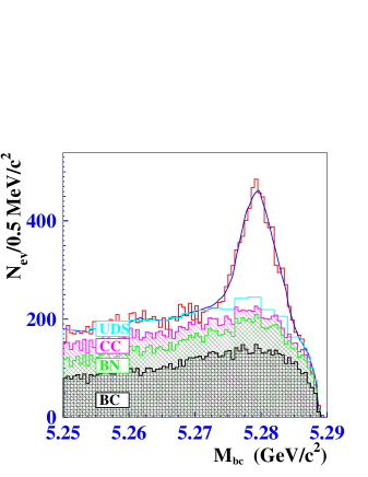
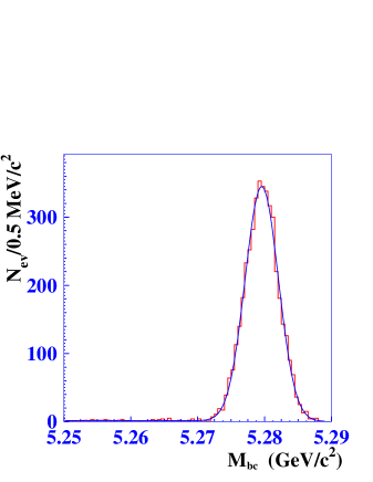
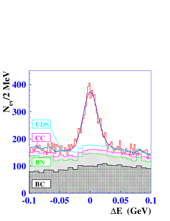
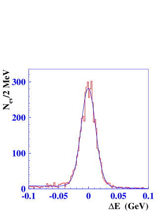
a)	b)
c)	d)

Figure 3: $M_{\rm bc}$ and $\Delta E$ distributions for $\bar{B}^{0}\to D^{0}\pi^{+}\pi^{-}$ events. Sample (1) distributions are shown in (a) and (c); those for sample (2) are shown in (b) and (d).

The fitted signal yields are $2909\pm 115$ events and $4202\pm 67$ events for samples (1) and (2), respectively. The reconstruction efficiencies $(23.4\pm 0.4)\%$ and $(19.0\pm 0.4)\%$ are determined from a MC simulation that uses a Dalitz plot distribution that is generated according to the model described in the next section. Taking into account ${\cal B}(D^{0}\to K^{-}\pi^{+})=(3.80\pm 0.07)\%$ PDG , we obtain the following branching fraction:

$${\cal B}(\bar{B}^{0}\to D^{0}\pi^{+}\pi^{-})=(8.4\pm 0.4\pm 0.8)\times 10^{-4},$$

where the first error is statistical and second error is systematic. Various contributions to the systematic error are listed in Table 1 for both samples. They include tracking efficiency, particle identification efficiency, limited MC statistics, and background uncertainty. The background uncertainty is obtained by varying the relative weights within their errors. The contribution of the non-resonant $\bar{B^{0}}\to K^{-}\pi^{+}\pi^{-}\pi^{+}$ is estimated using the $K\pi$ mass sidebands of the $D$ mass region and is negligible.

	sample(1)	sample(2)
Particle identification	$5\%$	$5\%$
Background uncertainty	$5\%$	$1\%$
Tracking efficiency	$4.4\%$	$5.4\%$
MC statistics	$3\%$	$3\%$
${\cal B}(D,D^{*})$ uncertainty	$2.4\%$	$2.5\%$
Total	$9.2\%$	$8.1\%$

Table 1: The systematic uncertainties for the $\bar{B}^{0}\to D^{0}\pi^{+}\pi^{-}$ branching fraction measurement.

The value of ${\cal B}(\bar{B}^{0}\to D^{0}\pi^{+}\pi^{-})$ improves and supersedes previous Belle result ${\cal B}(\bar{B}^{0}\to D^{0}\pi^{+}\pi^{-})=(8.0\pm 1.6)\times 10^{-4}$ Asish . The value of the branching fraction ${\cal B}(\bar{B}^{0}\to D^{*+}\pi^{-})$ is obtained using sample (2) and the PDG value ${\cal B}(D^{*+}\to D^{0}\pi^{+})=(67.7\pm 0.5)\%$ PDG . The result is ${\cal B}(\bar{B}^{0}\to D^{*+}\pi^{-})=(2.22\pm 0.04\pm 0.19)\times 10^{-3},$ which is somewhere lower than the CLEO result ${\cal B}(\bar{B}^{0}\to D^{*+}\pi^{-})=(2.81\pm 0.25)\times 10^{-3}$ CLEOd1 .

IV.1 $B\to D\pi\pi$ Dalitz plot analysis

For a three-body decay of a spin zero particle, two variables are required to describe the decay kinematics; we use the $D^{0}\pi^{+}$ and $\pi^{+}\pi^{-}$ invariant masses squared, $M^{2}_{D\pi}$ and $M^{2}_{\pi\pi}$, respectively.

To analyze the dynamics of $B\to D\pi\pi$ decays, sample (1) events with $\Delta E$ and $M_{\rm bc}$ within the signal region $((\Delta E+\kappa(M_{\rm bc}-m_{B}))/\sigma_{\Delta E})^{2}+((M_{\rm bc}-m_{B})/\sigma_{M_{\rm bc}})^{2}<4$ are selected. The parameters $\sigma_{\Delta E}=11~{}{\rm MeV},~{}\sigma_{M_{\rm bc}}=2.7~{}{\rm MeV}/c^{2}$ and $\kappa=0.9$ are determined from a fit to experimental data; the coefficient $\kappa$ accounts for the correlation between $M_{\rm bc}$ and $\Delta E$.

To test and correct the shape of the background, we use events from the $\Delta E$ sidebands, which are defined as: $((\Delta E\pm 65\,{\rm MeV}+\kappa(M_{\rm bc}-m_{B}))/\sigma_{\Delta E})^{2}+((M_{\rm bc}-m_{B})/\sigma_{M_{\rm bc}})^{2}<4$. Figure 4 shows the signal and sideband regions in the $M_{\rm bc}$-$\Delta E$ plane.

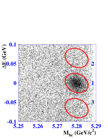
Figure 4: The experimental distribution in the $(M_{\rm bc}$-$\Delta E)$ plane. The ellipses show the signal (1) and sideband regions (2 & 3).

The $D\pi$ and $\pi\pi$ mass distributions for the signal and sideband events (sample 1) are shown in Fig. 5. In the $D\pi$ mass distribution a narrow peak corresponding to $D_{2}^{*}$ is evident. The $\pi\pi$ mass distribution shows a peak corresponding to the $\rho$ meson as well as a structure at the $1.2-1.3\,\rm GeV/c^{2}$ mass region that is presumably due to $f_{0}(1370)$ and $f_{2}(1270)$ production.

The $M^{2}_{D\pi}$ and $M^{2}_{\pi\pi}$ Dalitz plot distributions for the signal and sideband regions are shown in Fig. 6. The Dalitz plot boundary is fixed by the decay kinematics and the masses of the daughter particles. In order to have the same Dalitz plot boundary for both signal and sideband event samples, fits where the $K\pi$ mass is constrained to $M_{D}$ and $D\pi\pi$ mass to $m_{B}$ are performed. The mass-constrained fits also slightly improve the accuracy of $M^{2}_{D\pi}$ and $M^{2}_{\pi\pi}$.

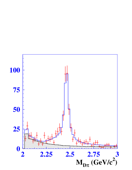
a)	b)

Figure 5: $D\pi$ (a) and $\pi\pi$ (b) mass distributions for sample (1) events with helicity angles $\cos\theta_{h}>0$. The points with error bars correspond to the signal region events, the hatched region indicates the background obtained from generic MC events normalized to the sideband data. The open histogram shows the fitted function after efficiency correction.

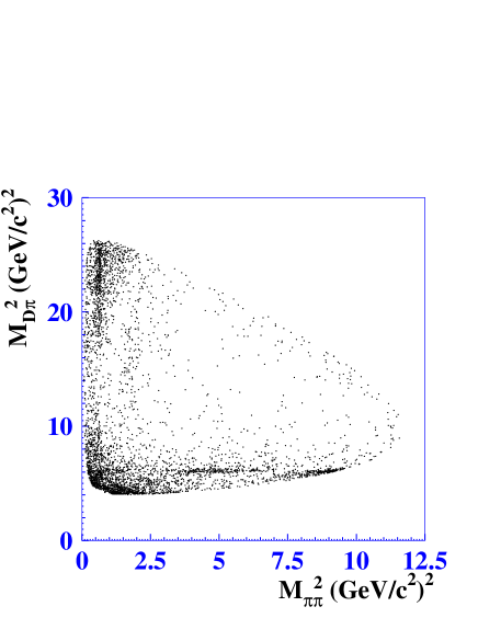
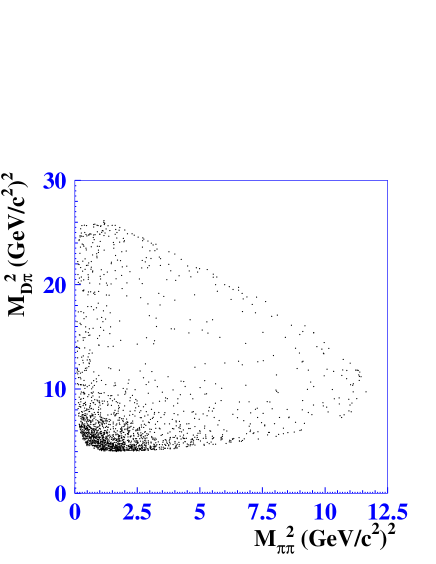
a)	b)

Figure 6: The Dalitz plot for (a) signal events; (b) sideband events.

To extract the amplitudes and phases of different intermediate states, an unbinned fit to the Dalitz plot is performed using the method described in Ref. mybelle . The event density function in the Dalitz plot includes both the signal and background functions.

The backgrounds in the Dalitz plot are mostly combinatorial and have neither resonant structure (Fig. 6b) nor specific helicity behavior. The background shape is obtained from an unbinned fit to $\Delta E$ sideband events using the weights described above. The background Dalitz plot density is modeled by a smooth two-dimensional function. The number of background events in the signal region is scaled according to the relative areas of the signal and sideband regions.

There is no general method to describe a three-body amplitude. In this paper we represent the $D\pi\pi$ amplitude as the sum of Breit-Wigner function contributions for different intermediate two-body states. Such an approach is not exact because it is neither analytic nor unitary and does not take into account a complete description of the final state interactions. Nevertheless, the sum of Breit-Wigner functions describes the main features of the amplitude behavior and allows one to find and distinguish the contributions of two-body intermediate states, their interference, and the effective parameters of these states. We followed the same approach in the analysis of charged $B$ decays mybelle .

In the $D^{0}\pi^{+}\pi^{-}$ final state, a combination of the $D^{0}$-meson and a pion can form a vector meson $D^{*+}$, a tensor meson $D^{*+}_{2}$ or a scalar state $D_{0}^{*+}$; the axial vector mesons $D_{1}^{+}$ and $D^{\prime+}_{1}$ cannot decay to two pseudoscalars because of angular momentum and parity conservation. The region of $D^{0}\pi^{+}$ invariant mass that corresponds to the $D^{*+}$ is excluded from the fit by requiring $|M_{D\pi}-M_{D^{*}}|>3$ MeV/c². However, in $B$-meson decay, a virtual $D^{*+}$ (referred to as $D^{*}_{v}$) can be produced off-shell with $M_{D\pi}$ above the $D^{0}\pi^{+}$ production threshold and such a process can contribute to the amplitude. Another virtual hadron that can be produced in this combination is $B^{*-}$ (referred to as $B^{*}_{v}$): $B\to B^{*}_{v}\pi$ and $B^{*}_{v}\to D\pi$. For the mass of ${B}^{*-}$ as well as the mass and width of the $D^{*+}$, we use the PDG values PDG ; the widths of ${B}^{*-}$ are calculated from the width of the $D^{*-}$ in the HQET approach. To describe the $\pi\pi$ system we include $\rho$, $\omega$, $f_{2}(1270)$, and three scalar mesons $f_{0}(600),~{}f_{0}(1370)$ and $f_{0}(980)$. The masses and widths of the $\rho$, $\omega$ and $f_{2}(1270)$ mesons are fixed at their PDG values; the parameters of the scalar mesons are taken from the published papers on the $f_{0}(600)$ f600 , $f_{0}(1370)$ f980 and $f_{0}(980)$ f980 .

The contributions from the intermediate states listed above are included in the signal-event density ($S(q^{2},q^{2}_{1})$) parameterization as a coherent sum of the corresponding amplitudes together with a possible constant amplitude ($a_{ps}$). The phases of the amplitudes are defined relative to $D_{2}^{*}$:

$$S(q^{2},q_{1}^{2}) = |a_{D^{*}_{2}}A^{D^{*}_{2}}(q^{2},q_{1}^{2})+a_{D^{*}_{0}}e^{i\phi_{D^{*}_{0}}}A^{D^{*}_{0}}(q^{2},q_{1}^{2})+a_{D^{*}_{v}}e^{i\phi_{D^{*}_{v}}}A^{D^{*}_{v}}(q^{2},q_{1}^{2})$$ (1)

$$+a_{\rho}e^{i\phi_{\rho}}(A^{\rho}(q^{2},q_{1}^{2})+r_{\omega-\rho}e^{i\phi_{\omega}}A^{\omega}(q^{2},q_{1}^{2}))+a_{f_{2}}e^{i(\phi_{f_{2}}+\phi_{\rho})}A^{f_{2}}(q^{2},q_{1}^{2})$$

$$+a_{f_{0}(600)}e^{i(\phi_{f_{0}(600)}+\phi_{\rho})}A^{f_{0}(600)}(q^{2},q_{1}^{2})+a_{f_{0}(980)}e^{i(\phi_{f_{0}(980)}+\phi_{\rho})}A^{f_{0}(980)}(q^{2},q_{1}^{2})$$

$$+a_{f_{0}(1470)}e^{i(\phi_{f_{0}(1470)}+\phi_{\rho})}A^{f_{0}(1470)}(q^{2},q_{1}^{2})+a_{B^{*}}e^{i\phi_{B^{*}_{v}}}A^{B^{*}_{v}}(q^{2},q_{1}^{2})+a_{ps}e^{i\phi_{ps}}|^{2},$$

where $q^{2}\equiv M^{2}_{D\pi}$ and $q_{1}^{2}\equiv M^{2}_{\pi\pi}$. The relative amplitude and phase of the $\omega$ meson are expressed via those of the $\rho$ meson. The relative phase is taken from $\rho$-$\omega$ interference measurements CMD2 , and the relative amplitude $(r_{\omega-\rho}=a_{\omega}/a_{\rho})$ is recalculated using that value. Assuming that the $\rho$ and $\omega$ mesons produced in $B^{0}$ decay emerge from the $d\bar{d}$ pair, the relative amplitude is expected to satisfy a relation $r_{\omega-\rho\,(B)}=-3r_{\omega-\rho\,(\gamma)}$.

We use the approach described in mybelle , where each resonance is described by a relativistic Breit-Wigner function with a $q^{2}$ dependent width and an angular dependence that corresponds to the spin and parity of the intermediate- and final-state particles. The $\rho$ meson amplitude is described by the Gounaris-Sakurai parameterization GS . We take into account transition form factors for hadron transitions using the Blatt-Weisskopf parameterization blat with a hadron scale $r$=1.6 $\rm(GeV/c)^{-1}$.

The variation of the detection efficiency over the Dalitz plot is taken into account by the minimization procedure. The efficiency dependence enters the likelihood function only through the normalization term. The normalization is obtained based on a large MC sample generated uniformly over the Dalitz plane, processed with the same selection criteria as the data and multiplied with the model used to fit the data. The detector resolution for the invariant mass of the $D\pi$($\pi\pi$) combination is about $2.5$ (3.5) MeV/c², which is much smaller than the narrowest peak width of 30–40 MeV/c². Hence convolution of the described parametrization with the resolution is not necessary. The mass and width of the broad $(D\pi)$ resonance, $M_{D_{0}^{*+}}=2308\,\rm MeV/c^{2},~{}\Gamma^{0}_{D_{0}^{*+}}=276\,{\rm MeV}/c^{2}$ are taken from our $D^{**0}$ measurement mybelle .

Table 2 gives the fit results for different models. The contributions of different states are characterized by their fractions, which are defined as:

$${f}_{i}=\frac{a_{i}^{2}\int|A_{i}(Q)|^{2}dQ}{\int|\sum_{k}a_{k}e^{i\phi_{k}}A_{k}(Q)|^{2}dQ},$$ (2)

where $A_{i}(Q)$ is the corresponding amplitude, and $a_{i}$ and $\phi_{i}$ are the amplitude coefficients and phases obtained from the fit. The integration is performed over all available phase space characterized by the multidimensional vector $Q$ (for decay to 3 spinless particles, $dQ\equiv dq^{2}dq_{1}^{2}$), and $i$ is one of the intermediate states: $D^{*}_{2},~{}D^{*}_{0},~{}\rho,~{}f_{2},~{}f_{0},~{}D^{*}_{v},~{}B^{*}_{v}$ or the constant term $a_{ps}$. The sum of the individual fractions ${f_{i}}$ exceeds unity for our case because of destructive interference. The product of the branching fractions of the $B$ meson is expressed via the fraction ${f}_{i}$:

$${\cal B}_{B\to i\pi}{\cal B}_{i\to D\pi}=\frac{N_{\rm sig}{f}_{i}}{N_{B\bar{B}}},$$ (3)

where $N_{\rm sig}$ is the efficiency corrected number of the reconstructed $D\pi\pi$ events and $N_{B\bar{B}}$ is the number of ${B\bar{B}}$ pairs produced.

Options	1	2	3	4	5
States	$D^{*}_{2},~{}D^{*}_{0},~{}D^{*}_{v},$	$D^{*}_{2},~{}D^{*}_{0},$	$D^{*}_{2},~{}D^{*}_{0},~{}D^{*}_{v},$	$D^{*}_{2},~{}D^{*}_{0},~{}D^{*}_{v},$	$D^{*}_{2},~{}D^{*}_{v},$
	$\rho,~{}f_{2},~{}f_{0}^{\prime}s$	$\rho,~{}f_{2},~{}f_{0}^{\prime}s$	$\rho,~{}f_{2},~{}f_{0}^{\prime}s,~{}B^{*}_{v}$	$\rho,~{}f_{2},~{}f_{0}^{\prime}s+ps$	$\rho,~{}f_{2},~{}f_{0}^{\prime}s$
$-2\ln{\cal L}/{\cal L}_{0}$	0	69.5	-2.7	-13.0	51.3
$N_{1}$	$2181\pm 64$	$2174\pm 64$	$2223\pm 71$	$2264\pm 65$	$2111\pm 62$
${\cal B}_{B\to D_{2}^{*}\pi}{\cal B}_{D_{2}^{*}\to D\pi}(10^{-4})$	$2.15\pm 0.16$	$2.23\pm 0.12$	$2.15\pm 0.18$	$2.26\pm 0.18$	$2.51\pm 0.14$
$M_{D^{*}_{2}},(MeV/c^{2})$	$2465.7\pm 1.7$	$2461.9\pm 1.6$	$2465.2\pm 1.9$	$2464.9\pm 1.6$	$2465.5\pm 1.7$
$\Gamma_{D^{*}_{2}},(MeV/c^{2})$	$49.6\pm 3.9$	$49.0\pm 3.9$	$49.3\pm 4.1$	$51.5\pm 3.8$	$55.4\pm 4.0$
${\cal B}_{B\to D_{0}^{*}\pi}{\cal B}_{D_{0}^{*}\to D\pi}(10^{-4})$	$0.60\pm 0.13$	$0.61\pm 0.10$	$0.50\pm 0.13$	$0.79\pm 0.11$	$0$
$\phi_{D_{0}^{*}}$	$-3.00\pm 0.13$	$-2.28\pm 0.17$	$-2.88\pm 0.17$	$-2.66\pm 0.11$	$0$
$M_{D^{*}_{0}},(MeV/c^{2})$	$2308.0$	$2308.0$	$2308.0$	$2308.0$	$2308.0$
$\Gamma_{D^{*}_{0}},(MeV/c^{2})$	$276.0$	$276.0$	$276.0$	$276.0$	$276.0$
${\cal B}_{B\to D_{v}^{*}\pi}{\cal B}_{D_{v}^{*}\to D\pi}(10^{-4})$	$0.88\pm 0.13$	$0$	$0.85\pm 0.14$	$0.74\pm 0.11$	$0.66\pm 0.10$
$\phi_{D^{*}_{v}}$	$-2.62\pm 0.15$	$0$	$-2.53\pm 0.17$	$-2.59\pm 0.13$	$-3.04\pm 0.20$
${\cal B}_{B\to D\rho}{\cal B}_{\rho\to\pi\pi}(10^{-4})$	$3.19\pm 0.20$	$2.94\pm 0.15$	$3.15\pm 0.21$	$3.07\pm 0.14$	$3.26\pm 0.18$
$\phi_{\rho}$	$2.25\pm 0.19$	$1.45\pm 0.22$	$1.81\pm 0.31$	$1.73\pm 0.15$	$1.89\pm 0.15$
$M_{\rho},(MeV/c^{2})$	$775.6$	$775.6$	$775.6$	$775.6$	$775.6$
$\Gamma_{\rho},(MeV/c^{2})$	$144.0$	$144.0$	$144.0$	$144.0$	$144.0$
${\cal B}_{B\to Df_{2}}{\cal B}_{f_{2}\to\pi\pi}(10^{-4})$	$0.68\pm 0.10$	$0.64\pm 0.08$	$0.64\pm 0.09$	$0.54\pm 0.08$	$0.65\pm 0.08$
$\phi_{f_{2}}$	$2.97\pm 0.21$	$2.48\pm 0.16$	$2.77\pm 0.20$	$2.32\pm 0.13$	$2.91\pm 0.17$
$M_{f_{2}},(MeV/c^{2})$	$1275.0$	$1275.0$	$1275.0$	$1275.0$	$1275.0$
$\Gamma_{f_{2}},(MeV/c^{2})$	$185.0$	$185.0$	$185.0$	$185.0$	$185.0$
${\cal B}_{B\to Df_{0}(600)}{\cal B}_{f_{0}(600)\to\pi\pi}(10^{-4})$	$0.68\pm 0.08$	$0.72\pm 0.09$	$0.72\pm 0.09$	$0.47\pm 0.08$	$0.58\pm 0.07$
$\phi_{f_{0}(600)}$	$-0.44\pm 0.09$	$-0.42\pm 0.09$	$-0.40\pm 0.10$	$-0.43\pm 0.11$	$-0.32\pm 0.10$
$M_{f_{0}},(MeV/c^{2})$	$513.0$	$513.0$	$513.0$	$513.0$	$513.0$
$\Gamma_{f_{0}},(MeV/c^{2})$	$335.0$	$335.0$	$335.0$	$335.0$	$335.0$
${\cal B}_{B\to Df_{0}(980)}{\cal B}_{f_{0}(980)\to\pi\pi}(10^{-4})$	$0.08\pm 0.04$	$0.11\pm 0.04$	$0.08\pm 0.04$	$0.04\pm 0.02$	$0.08\pm 0.03$
$\phi_{f_{0}(980)}$	$-2.48\pm 0.47$	$2.68\pm 0.37$	$-3.07\pm 0.51$	$2.87\pm 0.37$	$-2.85\pm 0.32$
$M_{f_{0}},(MeV/c^{2})$	$978.0$	$978.0$	$978.0$	$978.0$	$978.0$
$\Gamma_{f_{0}},(MeV/c^{2})$	$44.0$	$44.0$	$44.0$	$44.0$	$44.0$
${\cal B}_{B\to Df_{0}(1370)}{\cal B}_{f_{0}(1370)\to\pi\pi}(10^{-4})$	$0.21\pm 0.10$	$0.24\pm 0.06$	$0.18\pm 0.06$	$0.15\pm 0.04$	$0.25\pm 0.10$
$\phi_{f_{0}(1370)}$	$-1.52\pm 0.56$	$3.08\pm 0.35$	$-2.43\pm 0.62$	$-2.75\pm 0.28$	$-2.00\pm 0.38$
$M_{f_{0}},(MeV/c^{2})$	$1434.0$	$1434.0$	$1434.0$	$1434.0$	$1434.0$
$\Gamma_{f_{0}},(MeV/c^{2})$	$173.0$	$173.0$	$173.0$	$173.0$	$173.0$
${\cal B}_{B\to B^{*}_{v}\pi}{\cal B}_{B^{*}_{v}\to D\pi}(10^{-4})$	0	0	$0.74\pm 0.76$	0	0
$\phi_{B^{*}_{v}}$	0	0	$1.09\pm 0.51$	0	0
$\phi_{ps}$	0	0	0	$0.22\pm 0.14$	0
${\cal B}_{ps}(10^{-4})$	0	0	0	$0.33\pm 0.18$	0
$\chi^{2}/N_{dof}$	629/603	680/605	632/601	618/601	659/605
$CL~{}(\%)$	23	1.8	18	31	6.3

Table 2: The fit results for different sets of amplitudes. Option 1 is used as the main set of amplitudes for the final results.

Table 2 contains information on the likelihood change relative to the main set, and $\chi^{2}$ values obtained from four histograms: projections of $M_{D\pi}$ and $M_{\pi\pi}$ for negative and positive helicities of the $D\pi$ and $\pi\pi$ systems, respectivelyfootchi .

The fit gives a statistically significant contribution from off-shell $D^{*}_{v}\pi$ production; the addition of the off-shell $B^{*}_{v}$ amplitude does not improve the likelihood value significantly. The inclusion of the three-particle phase space term improves the likelihood value, however there is no reason to expect a constant amplitude with no momentum dependence over such a wide range of final particle momenta. Table 3 shows that the likelihood changes significantly when the broad resonance $D^{*}_{0}$ is removed or treated as either a vector or a tensor. The change of likelihood $-2\ln{\cal L}/{\cal L}_{0}=51$ for 2 additional degrees of freedom (amplitude and phase of $D^{*}_{0}$) corresponds to a significance of 6.8 $\sigma$ wilk .

The branching fractions of $D^{*}_{2}$ and $D_{0}^{*}$ remain constant within errors for different models. The set of states used for the final results are $D^{*}_{2},~{}D^{*}_{0},~{}D^{*}_{v},~{}\rho,~{}f_{2}$ and the three above-listed $f_{0}$’s listed above, corresponding to column 1 in Table 2.

The values of the $D_{2}^{*+}$ resonance mass and width obtained from the fit are:

$$M_{D^{*+}_{2}}=(2465.7\pm 1.8\pm 0.8^{+1.2}_{-4.7}){\,\rm MeV}/c^{2},~{}~{}\Gamma_{D^{*+}_{2}}=(49.7\pm 3.8\pm 4.1\pm 4.9){\,\rm MeV},$$

where the third error is model uncertainty. These parameters are consistent with but more precise than previous measurements performed by CLEO $M_{D^{*0}_{2}}=(2463\pm 3\pm 3)\,{\rm MeV}/c^{2}$ dobs and FOCUS $~{}\Gamma_{D^{*}_{2}}=(34.1\pm 6.5\pm 4.2)\,\rm{MeV}$ FOC .

The product of the branching fraction for $D^{*}_{2}$ production obtained from the fit is:

$${\cal B}(\bar{B}^{0}\to D^{*+}_{2}\pi^{-})\times{\cal B}(D_{2}^{*+}\to D^{0}\pi^{+})=(2.15\pm 0.17\pm 0.29\pm 0.12)\times 10^{-4},$$

where the three errors are statistical, systematic, and a model-dependent error, respectively. We observe the production of the broad scalar $D_{0}^{*+}$ state with the product branching fraction,

$${\cal B}(\bar{B}^{0}\to D^{*+}_{0}\pi^{-})\times{\cal B}(D_{0}^{*+}\to D^{0}\pi^{+})=(0.60\pm 0.13\pm 0.15\pm 0.22)\times 10^{-4}.$$

This is the first observation of this decay (the interpretation of the neutral partner of this state is still a subject of theoretical discussion tfoc ). The relative phase of the $D_{0}^{*}$ amplitude is

$$\phi_{0}=3.00\pm 0.13\pm 0.10\pm 0.43.$$

The $D\pi$ helicity angle distributions for $M_{D\pi}$ regions corresponding to the $D^{*}_{2}$ and $D^{*}_{0}$ are shown in Fig. 7(a) and (b), respectively, together with the efficiency-corrected fitting function. The histogram in the region of the $D^{*}_{2}$ meson clearly indicates a D-wave. The distributions in the other regions show reasonable agreement between the fitting function and the data.

	no broad state	$0^{+}$	$1^{-}$	$2^{+}$
$-2\ln{\cal L}/{\cal L}_{0}$	51	0	28	27
$\chi^{2}/N_{dof}$	659/605	629/603	652/603	640/603
$CL,~{}(\%)$	6.3	22	8.1	14

Table 3: Changes in likelihood for different quantum number assignments for the broad resonance.

The uncertainty of the background is one of the main sources of systematic error. This is estimated by comparing the fit results for the case when the background shape is taken separately from the lower or upper $\Delta E$ sidebands. The fit is also performed with more restrictive and looser cuts on $\Delta E$, $M_{\rm bc}$ and $\Delta M_{D}$ that change the signal-to-noise ratio by factors of about two. The results obtained are consistent with each other and the maximum difference is taken as an additional estimate of the systematic uncertainty. The systematic errors on the ${\cal B}_{i}$ measurements (Eq. (3)) for the individual intermediate states include uncertainties in track reconstruction and PID efficiency, as well as the error in the $D^{0}\to K^{-}\pi^{+}$ absolute branching fraction. The model uncertainties are estimated by comparing fit results for the case of different models and for values of the parameter $r$ of the transition form factor blat from 0 to 3 (GeV/$c$)^-1.

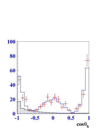
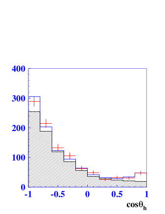
a)	b)

Figure 7: $D\pi$ helicity angle distributions for data (points) and MC (histogram). The hatched distribution shows the background from the $\Delta E$ sideband region with the appropriate normalization. (a) corresponds to the $D^{*}_{2}$ region $|M_{D\pi}-2.46|<0.1\rm\,GeV/c^{2}$; (b) the $D_{0}$ region $|M_{D\pi}-2.30|<0.1\rm\,GeV/c^{2}$.

The $\pi\pi$ helicity angle distributions for $M_{\pi\pi}$ ranges corresponding to the $\rho$, $f_{2}$ and the region below the $\rho$, where the broad resonance dominates, are shown in Fig. 8. For the positive helicity region, where the $D\pi$ contribution is suppressed, a clear $P$-wave structure for the $\rho$ and $D$-wave structure for the $f_{2}$ is observed. The scalar component parameters cannot be determined from the fit. This process can also have contributions from non-resonant background. The product branching fraction for the $f_{2}$ is

$${\cal B}(\bar{B}^{0}\to D^{0}f_{2}){\cal B}(f_{2}\to\pi^{+}\pi^{-})=(0.68\pm 0.10\pm 0.12\pm 0.18)\times 10^{-4}.$$

Taking into account the branching fraction ${\cal B}(f_{2}\to\pi\pi)=$ $0.847^{+0.025}_{-0.012}$ PDG and the corresponding Clebsch-Gordan coefficients, we obtain

$${\cal B}(\bar{B}^{0}\to D^{0}f_{2})=(1.20\pm 0.18\pm 0.21\pm 0.32)\times 10^{-4},$$

$${\cal B}(\bar{B}^{0}\to D^{0}\rho^{0})=(3.19\pm 0.20\pm{0.24}\pm 0.38)\times 10^{-4}.$$

The phases relative to the $D_{2}^{*}$ amplitude are $\phi_{\rho}=2.25\pm 0.19\pm 0.20^{+0.21}_{-0.99}$ and $~{}\phi_{f_{2}}=2.97\pm 0.21\pm 0.13\pm{0.45}.$

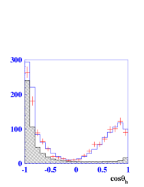
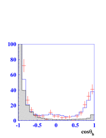
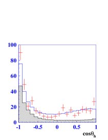
a)	b)	c)

Figure 8: $\pi\pi$ helicity angle distributions for data (points) and MC (histogram). The hatched distribution shows the background distribution from the $\Delta E$ sideband region with appropriate normalization. (a) corresponds to the $\rho$ region $|M_{\pi\pi}-0.78|<0.2\,$GeV/$c^{2}$; (b) the $f_{2}$ region $|M_{\pi\pi}-1.20|<0.1\,$GeV/$c^{2}$; (c) the $f_{0}$ region $M_{\pi\pi}<0.60\,$GeV/$c^{2}$.

IV.2 Results and discussion

The branching fraction products obtained for the narrow $(j=3/2)$ resonances are similar to the published results for charged $B$ decays as shown in Table 4.

	neutral $B$	charged $B$ mybelle
${\cal B}(\bar{B}\to D^{*}_{2}\pi^{-}){\cal B}(D_{2}^{*}\to D\pi)$	$(2.15\pm 0.17\pm 0.29\pm 0.12)\times 10^{-4}$	$(3.4\pm 0.3\pm 0.6\pm 0.4)\times 10^{-4}$
${\cal B}(\bar{B}\to D^{*}_{2}\pi^{-}){\cal B}(D_{2}^{*}\to D^{*}\pi)$	$(2.45\pm 0.42^{+0.35+0.39}_{-0.45-0.17})\times 10^{-4}$ hhh	$(1.8\pm 0.3\pm 0.3\pm 0.2)\times 10^{-4}$
${\cal B}(\bar{B}\to D_{1}\pi^{-}){\cal B}(D_{1}\to D^{*}\pi)$	$(3.68\pm 0.60^{+0.71+0.65}_{-0.40-0.30})\times 10^{-4}$ hhh	$(6.8\pm 0.7\pm 1.3\pm 0.3)\times 10^{-4}$
${\cal B}(\bar{B}\to D^{*}_{0}\pi){\cal B}(D_{0}^{*}\to D\pi)$	$(0.60\pm 0.13\pm 0.15\pm 0.22)\times 10^{-4}$	$(6.1\pm 0.6\pm 0.9\pm 1.6)\times 10^{-4}$
${\cal B}(\bar{B}\to D^{\prime}_{1}\pi^{-}){\cal B}(D^{\prime}_{1}\to D^{*}\pi)$	$<0.7\times 10^{-4}\rm~{}at~{}90\,\%~{}C.L.$ hhh	$(5.0\pm 0.4\pm 1.0\pm 0.4)\times 10^{-4}$

Table 4: Comparison of product branching fractions for neutral and charged $B$ decays.

The measured values of the branching fractions for the broad $D^{*+}_{0}$ resonances in neutral $B$ decays are, however, significantly lower than those for charged $B$ decays. Preliminary data on $\bar{B^{0}}\to D^{*0}\pi^{+}\pi^{-}$ decay hhh shown in Table 4 indicates a similar behavior for $D^{\prime 0}_{1}$ and $D_{1}^{0}$ production. One possible explanation for this phenomenon is that for charged $B$ decay to $D^{**}\pi$, the amplitude receives contributions from both tree and color-suppressed diagrams as shown in Fig. 2. For the color-suppressed diagrams, however, $D^{**}$’s are produced by another mechanism and the amplitudes are characterized by the constants $f_{D(3/2)}$ and $f_{D(1/2)}$, with $f_{D(3/2)}\ll f_{D(1/2)}$. The production of the broad resonances $D^{*0}_{0}$ and $D^{\prime 0}_{1}$ in charged $B$ decay is amplified by the color-suppressed amplitude. As shown in yon2 , in such a case both $\tau_{1/2}$ fits to the sum rule and the value of $f_{D(1/2)}$ are consistent with theoretical estimates.

V Conclusion

A study of neutral $B$-meson decays to $D^{0}\pi^{+}\pi^{-}$ is reported. We measure the total branching fraction of the three-body $D^{0}\pi^{+}\pi^{-}$ decays, obtaining ${\cal B}(\bar{B}^{0}\to D^{0}\pi^{+}\pi^{-})=(8.4\pm 0.4\pm 0.8)\times 10^{-4}$. The intermediate resonant structure of these three-body decays is studied. The $D^{0}\pi^{+}\pi^{-}$ final state is described by the production of $D^{*}_{0,2}\pi^{-}$ with subsequent decays $D^{*}_{0,2}\to D\pi$, and also by $D\rho,~{}Df_{2}$, and $D\sigma$, where $\sigma$ is a broad scalar ($\pi\pi$) structure. From a Dalitz plot analysis we obtain the mass, width and product of the branching fractions for the $D^{*+}_{2}$:

$$M_{D^{*+}_{2}}=(2465.7\pm 1.8\pm 0.8^{+1.2}_{-4.7}){\rm MeV}/c^{2},~{}~{}\Gamma_{D^{*+}_{2}}=(49.7\pm 3.8\pm 4.1\pm 4.9){\rm MeV},$$

$${\cal B}(\bar{B}^{0}\to D^{*+}_{2}\pi^{-})\times{\cal B}(D_{2}^{*+}\to D^{0}\pi^{+})=(2.15\pm 0.17\pm 0.29^{\pm}0.12)\times 10^{-4}.$$

We observe the production of the broad scalar $D_{0}^{*+}$ state with the product branching fraction

$${\cal B}(\bar{B}^{0}\to D^{*+}_{0}\pi^{-})\times{\cal B}(D_{0}^{*+}\to D^{0}\pi^{+})=(0.60\pm 0.13\pm 0.15\pm 0.22)\times 10^{-4}.$$

This is the first observation of this decay. The phase of the $D_{0}^{*}$ amplitude relative to that of the $D_{2}^{*}$ is determined to be:

$$\phi_{0}=3.00\pm 0.13\pm 0.10\pm 0.43.$$

The $B\to D\rho$ and $Df_{2}$ branching fractions are measured to be:

$${\cal B}(\bar{B}^{0}\to D^{0}\rho^{0})=(3.19\pm 0.20\pm{0.24}\pm 0.38)\times 10^{-4},$$

$${\cal B}(\bar{B}^{0}\to D^{0}f_{2})=(1.20\pm 0.18\pm 0.21\pm 0.32)\times 10^{-4},$$

and the phases relative to the $D_{2}^{*}$ amplitude are:

$$\phi_{\rho}=2.25\pm 0.19\pm 0.20^{+0.21}_{-0.99},$$

$$\phi_{f_{2}}=2.97\pm 0.21\pm 0.13\pm{0.45}.$$

This is the first observation of the $\bar{B^{0}}\to D^{0}f_{2}$ decay.

References

- (1) H. Albrecht et al. (ARGUS Collaboration), Phys. Rev. Lett. 56, 549 (1986).
- (2) H. Albrecht et al. (ARGUS Collaboration), Phys. Lett. B 221, 422 (1989).
- (3) H. Albrecht et al. (ARGUS Collaboration), Phys. Lett. B 232, 398 (1989).
- (4) J. C. Anjos et al. (Tagged Photon Spectrometer Collaboration), Phys. Rev. Lett. 62, 1717 (1989).
- (5) P. Avery et al. (CLEO Collaboration), Phys. Rev. D 41, 774 (1990).
- (6) P. L. Frabetti et al. (E687 Collaboration), Phys. Rev. Lett. 72, 324 (1994).
- (7) P. Avery et al. (CLEO Collaboration), Phys. Lett. B 331, 236 (1994) [Erratum-ibid. B 342, 453 (1995)].
- (8) T. Bergfeld et al. (CLEO Collaboration), Phys. Lett. B 340, 194 (1994).
- (9) D. Bloch et al. (DELPHI Collaboration), CERN-OPEN-2000-015, DELPHI-98-128-CONF-189, Jun 1998. 12pp. 29th International Conference on High-Energy Physics, Vancouver, Canada, 23-29 Jul 1998.
- (10) D. Bloch et al. (DELPHI Collaboration), DELPHI-2000-106-CONF 405.
- (11) D. Buskulic et al. (ALEPH Collaboration ), Z.Phys. C 73, 601 (1997).
- (12) N. Isgur and M.B. Wise, Phys. Rev. Lett. 66, 1130 (1991).
- (13) J. L. Rosner, Comm. Nucl. Part. Phys. 16, 109 (1986).
- (14) S. Godfrey and R. Kokoski, Phys. Rev. D 43, 1679 (1991).
- (15) A.F. Falk and M.E. Peskin, SLAC-PUB-6311 (1993).
- (16) N. Uraltsev, Phys. Lett. B 501, 86 (2001).
- (17) A. Le Yaouanc et al., Phys. Lett. B 520, 25 (2001).
- (18) K.Abe et al. (Belle Collaboration), Phys. Rev. D 69, 112002 (2004).
- (19) K. Abe et al., ( Belle Collaboration), hep-ex/0412072.
- (20) A. Abashian et al. (Belle Collaboration), Nucl. Instr. and Meth. A 479, 117 (2002).
- (21) Events are generated with a modified version of the CLEO group’s QQ program (http://www.lns.cornell.edu/public/CLEO/soft/QQ); the detector response is simulated using GEANT, R.Brun et al., GEANT 3.21, CERN Report DD/EE/84-1, 1984.
- (22) E. Nakano, Nucl. Instr. and Meth. A 494, 402 (2002).
- (23) W.-M. Yao et al. (Particle Data Group), J. Phys. G 33, 1 (2006).
- (24) The coordinate of the track is defined as the coordinate of the track point closest to the beam in the plane. The axis is opposite to the positron beam direction.
- (25) A.Satpathy et al. (Belle Collaboration), Phys. Lett. B 553, 159 (2003).
- (26) G. Brandenburg et al. (CLEO Collaboration), Phys. Rev. Lett. 80, 2762 (1998).
- (27) J. M. Link et al.(FOCUS Collaboration), Phys. Lett. B 586, 11 (2004).
- (28) H. Muramatsu et al., Phys. Rev. Lett. 89, 251802 (2002).
- (29) E. M. Aitala et al., Phys. Rev. Lett. 86, 765 (2001).
- (30) R. R. Akhmetshin et al. (CMD-2 Collaboration), Phys. Lett. B 527, 161 (2002).
- (31) G. J. Gounaris, J. J. Sakurai, Phys. Rev. Lett. 21, 244 (1986).
- (32) J. Blatt and V. Weisskopf, Theoretical Nuclear Physics, p.361, New York: John Wiley & Sons (1952).
- (33) S. S. Wilks, The Annals of Mathematical Statistic 9, 60 (1938).
- (34) The overall is calculated as the sum of the ’s from four distributions: two 160-bin histograms of for positive and negative helicities of the system, and two 150-bin histograms with positive and negative helicities of the system. The number of degrees of freedom is calculated as the number of bins minus the number of free parameters.
- (35) M. E. Bracco, A. Lozea, R. D. Matheus, F. S. Navarra and M. Nielsen, Phys. Lett. B 624, 217 (2005).
- (36) F. Jugeau, A. Le Yaouanc, L. Oliver and J. C. Raynal, Phys. Rev. D 72, 094010 (2005).