Separated Structure Functions for the Exclusive Electroproduction of $K^{+}\Lambda$ and $K^{+}\Sigma^{0}$ Final States

Abstract

We report measurements of the exclusive electroproduction of $K^{+}\Lambda$ and $K^{+}\Sigma^{0}$ final states from a proton target using the CLAS detector at the Thomas Jefferson National Accelerator Facility. The separated structure functions $\sigma_{T}$, $\sigma_{L}$, $\sigma_{TT}$, and $\sigma_{LT}$ were extracted from the $\Phi$- and $\epsilon$-dependent differential cross sections taken with electron beam energies of 2.567, 4.056, and 4.247 GeV. This analysis represents the first $\sigma_{L}/\sigma_{T}$ separation with the CLAS detector, and the first measurement of the kaon electroproduction structure functions away from parallel kinematics. The data span a broad range of momentum transfers from $0.5\leq Q^{2}\leq 2.8$ GeV² and invariant energy from $1.6\leq W\leq 2.4$ GeV, while spanning nearly the full center-of-mass angular range of the kaon. The separated structure functions reveal clear differences between the production dynamics for the $\Lambda$ and $\Sigma^{0}$ hyperons. These results provide an unprecedented data sample with which to constrain current and future models for the associated production of strangeness, which will allow for a better understanding of the underlying resonant and non-resonant contributions to hyperon production.

I Introduction

A necessary step toward understanding the structure and dynamics of strongly interacting matter is to fully understand the spectrum of excited states of the nucleon. This excitation spectrum is a direct reflection of its underlying substructure. Understanding nucleon resonance excitation, and hadro-production in general, continues to provide a serious challenge to hadronic physics due to the non-perturbative nature of the theory of strong interactions, Quantum Chromodynamics (QCD), at these energies. Because of this, a number of approximations to QCD have been developed to understand baryon resonance decays. One such approach is a class of semi-relativized symmetric quark models isgur ; capstick that invoke massive constituent quarks. These models typically predict many more nucleonic states than have been found experimentally. A possible explanation to this so-called “missing resonance” problem is that these nucleon resonances may have a relatively weak coupling to the pion-nucleon states through which many searches have been performed, and may, in fact, couple to other final states such as multi-pion or strangeness channels. In this work we provide an extensive set of data that may be used to search for these hidden states in strangeness electroproduction reactions. These data then provide for a complementary way in which to view the baryon resonance spectrum, as some of the “missing” states might be only “hidden” when studied in particular reactions. It could also be the case that some dynamical aspect of hadronic structure is acting to restrict the quark model spectrum of states to the more limited set established by existing data klempt .

Beyond different coupling constants relative to single-pion production (e.g. $g_{KYN}$ vs. $g_{\pi NN}$), the study of the exclusive production of $K^{+}\Lambda$ and $K^{+}\Sigma^{0}$ final states has other advantages in the search for missing resonances. The higher masses of the kaon and hyperons, compared to pionic final states, kinematically favor a two-body decay mode for resonances with masses near 2 GeV, a situation that is experimentally advantageous. New information is also provided by comparing $K^{+}\Lambda$ to $K^{+}\Sigma^{0}$. Note that although the two ground-state hyperons have the same valence quark structure ($uds$), they differ in isospin, such that intermediate $N^{*}$ resonances can decay strongly to $K^{+}\Lambda$ final states, but intermediate $\Delta^{*}$ states cannot. Because $K^{+}\Sigma^{0}$ final states can have contributions from both $N^{*}$ and $\Delta^{*}$ states, the hyperon final state selection constitutes an isospin filter.

Electro-excitation of the nucleon has served to quantify the structure of many excited states that decay to single pions. These studies have been used to test models of the internal structure of the excitations using the interference structure functions and the behavior with $Q^{2}$ for various regions of $W$. This experiment is the first to allow analogous investigations to start when the intermediate electro-excited nucleon resonances couple to kaon-hyperon final states.

The search for missing resonances requires more than identifying features in the relevant mass spectrum. It also requires an iterative approach in which experimental measurements constrain the dynamics of various hadrodynamic models. The tuned models can in turn be used to interpret $s$-, $t$- and $u$-channel spectra in terms of the underlying resonances. As emphasized by Lee and Sato lee , QCD cannot be directly tested with $N^{*}$ spectra without a model for the production dynamics. The key to constraining models and unraveling the contributing resonant and non-resonant diagrams that contribute to the dynamics, is to measure as many observables over as wide a kinematic range as possible.

In this paper, we present measurements of the separated structure functions $\sigma_{U}$, $\sigma_{TT}$, and $\sigma_{LT}$ for exclusive electroproduction of $K^{+}\Lambda$ and $K^{+}\Sigma^{0}$ final states for a range of momentum transfer $Q^{2}$ from 0.5 to 2.8 GeV² and invariant energy $W$ from 1.6 to 2.4 GeV, while spanning the full center-of-mass angular range of the kaon. Our center-of-mass angular coverage is unprecedented. These are the first data published on exclusive $KY$ electroproduction that extend beyond very forward kaon angles in the center of mass. At one value of $Q^{2}$, $Q^{2}$= 1.0 GeV², we were also able to separate the unpolarized structure function, $\sigma_{U}$, into its components $\sigma_{T}$ and $\sigma_{L}$ using a traditional Rosenbluth separation and also an alternative $\epsilon-\Phi$ Rosenbluth technique (where $\epsilon$ is the transverse polarization of the virtual photon and $\Phi$ is the angle between the electron and hadron planes). In this alternative method, we obtain the four structure functions in a single fit. This extensive data set should provide substantial constraints on the various hadrodynamic models (discussed in Section IV). Due to the very large number of analysis bins encompassed by this work, only a portion of our available data is included here. The full set of our data is available in Ref. database .

After a brief review of the relevant formalism in Section II, an overview of previous experimental work in this area in Section III, and a brief review of the current theoretical approaches in Section IV, we present our measurements made using the CLAS detector in Hall B at Jefferson Laboratory (JLab) in Sections V through VII. In Section VIII, the results are examined phenomenologically and compared to predictions from several models that have not been “tuned” to this data set. Finally, we present our conclusions regarding the potential impact of these data in Section IX. Our conclusions regarding the $s$-channel baryon spectrum are, unfortunately, rather limited. Real progress on identifying heretofore “missing” resonances will only result from a judicious fitting of the theoretical and phenomenological models to these data and the remainder of the world’s data on these final states.

II Formalism

In kaon electroproduction a beam of electrons with four-momentum $p_{e}=(E_{e},\vec{p}_{e}\,)$ is incident upon a fixed proton target of mass $M_{p}$, and the outgoing scattered electron with momentum $p_{e^{\prime}}=(E_{e^{\prime}},\vec{p}_{e^{\prime}}\,)$ and kaon with momentum $p_{K}=(E_{K},\vec{p}_{K})$ are measured. The cross section for the exclusive $K^{+}$-hyperon state is then differential in the scattered electron momentum and kaon direction. Under the assumption of single-photon exchange, where the photon has four-momentum $q=p_{e}-p_{e^{\prime}}=(\nu,\vec{q}\,)$, this can be re-expressed as the product of an equivalent flux of virtual photons and the $\gamma^{*}p$ center-of-mass (c.m.) virtual photo-absorption cross section as:

$$\frac{d\sigma}{dE_{e^{\prime}}d\Omega_{e^{\prime}}d\Omega_{K}^{*}}=\Gamma\frac{d\sigma_{v}}{d\Omega_{K}^{*}},$$ (1)

where the virtual photon flux factor $\Gamma$ depends upon only the electron scattering process. After integrating over the azimuthal angle of the scattered electron, the absorption cross section can be expressed in terms of the variables $Q^{2}$, $W$, $\theta_{K}^{*}$, and $\Phi$, where $q^{2}=-Q^{2}$ is the squared four-momentum of the virtual photon, $W=\sqrt{M_{p}^{2}+2M_{p}\nu-Q^{2}}$ is the total hadronic energy in the c.m. frame, $\theta_{K}^{*}$ is the c.m. kaon angle relative to the virtual photon direction, and $\Phi$ is the angle between the leptonic and hadronic production planes (see Fig. 1). After introducing the appropriate Jacobian, the form of the cross section can be written as:

$$\frac{d\sigma}{dQ^{2}dWd\Omega_{K}^{*}}=\Gamma_{v}\frac{d\sigma_{v}}{d\Omega_{K}^{*}},$$ (2)

where

$$\Gamma_{v}=\frac{\alpha}{4\pi}\frac{W}{M_{p}^{2}E^{2}}\frac{W^{2}-M_{p}^{2}}{Q^{2}}\frac{1}{1-\epsilon}$$ (3)

is the flux of virtual photons,

$$\epsilon=\left(1+2\frac{|\vec{q}\,|^{2}}{Q^{2}}\tan^{2}{\frac{\theta_{e^{\prime}}}{2}}\right)^{-1}$$ (4)

is the transverse polarization of the virtual photon, and $\theta_{e^{\prime}}$ is the electron scattering angle in the laboratory frame.

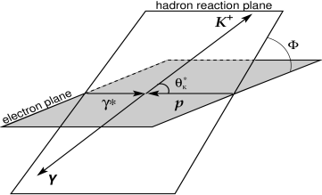
Figure 1: Kinematics for $K^{+}Y$ (where $Y$ is either a $\Lambda$ or $\Sigma^{0}$) electroproduction defining the angles $\theta_{K}^{*}$ and $\Phi$ with respect to the center-of-mass reference frame.

After summing over the polarizations of the initial and final state electrons and hadrons, the virtual photon cross section can be written as:

$$\frac{d\sigma_{v}}{d\Omega_{K}^{*}}=\sigma_{T}+\epsilon\sigma_{L}+\epsilon\sigma_{TT}\cos 2\Phi+\sqrt{\epsilon(\epsilon+1)}\sigma_{LT}\cos\Phi.$$ (5)

In this expression, the cross section is decomposed into four structure functions, $\sigma_{T}$, $\sigma_{L}$, $\sigma_{TT}$, and $\sigma_{LT}$, which are, in general, functions of $Q^{2}$, $W$, and $\theta_{K}^{*}$ only. Note that this convention for the differential cross section is not used by all authors convention .

Each of the structure functions is related to the coupling of the hadronic current to different combinations of the transverse and longitudinal polarization of the virtual photon. $\sigma_{T}=\frac{1}{2}(\sigma_{\parallel}+\sigma_{\perp})$ is the differential cross section contribution for unpolarized transverse virtual photons. In the limit $Q^{2}\to 0$, this term must approach the cross section for unpolarized real photons which only have transverse polarization. $\sigma_{L}$ is the differential cross section contribution for longitudinally polarized virtual photons. $\sigma_{TT}$ and $\sigma_{LT}$ represent interference contributions to the cross section. $\sigma_{TT}=\frac{1}{2}(\sigma_{\parallel}-\sigma_{\perp})$ is due to the interference of transversely polarized virtual photons and $\sigma_{LT}$ is due to the interference of transversely and longitudinally polarized virtual photons. Here $\sigma_{\parallel}$ and $\sigma_{\perp}$ are the cross sections for virtual photons having their electric vector parallel and perpendicular to the hadronic production plane, respectively. Note that the term $\sigma_{TT}$ in electroproduction is related to the linearly polarized photon beam asymmetry in photoproduction experiments, which is defined as $\Sigma=-\sigma_{TT}/\sigma_{T}$.

For the remainder of this paper we will refer to $\sigma_{U}=\sigma_{T}+\epsilon\sigma_{L}$ as the “unseparated” part of the cross section. The further decomposition of these structure functions into response functions, which can then be expressed in terms of either complex amplitudes or as multipole expansions, is given, for example, in Ref. knochlein . In this paper we will compare theory to the structure function terms introduced above.

III Previous Experimental Work

Hyperon electroproduction in the nucleon resonance region has remained largely unexplored. Several low-statistics measurements were carried out in the 1970’s at Cambridge, Cornell, and DESY, and focussed mainly on cross section measurements to explore differences in the production dynamics between $\Lambda$ and $\Sigma^{0}$ hyperons. The first experiment was performed at the Cambridge Electron Accelerator brown using small-aperture spectrometers in kinematics spanning $Q^{2}$ below 1.2 GeV², $W$ from 1.8 to 2.6 GeV, and forward kaon angles ($\theta_{K}^{*}<28^{\circ}$). It was noted that the $K^{+}\Lambda$ channel dominated the $K^{+}\Sigma^{0}$ channel, with signs of a large longitudinal component in the $K^{+}\Lambda$ channel. Subsequent results from Cornell bebek1 for $Q^{2}<$ 2.0 GeV² and $W$=2.15 and 2.67 GeV confirmed this observation. In this paper we show that $K^{+}\Lambda$ dominance only occurs at forward kaon angles, and the longitudinal strength is only important at forward angles and higher $W$.

An experiment from DESY azemoon used a large aperture spark-chamber spectrometer to measure both reaction channels at higher $W$ ($1.9<W<2.8$ GeV) and lower $Q^{2}$ ($0.1<Q^{2}<0.6$ GeV²). That experiment managed the first $\sigma_{LT}$ and $\sigma_{TT}$ separations, albeit with large error bars, few data points, and considerable kinematic extrapolations to extract results at fixed values of $W$, $Q^{2}$, and $t=(q-p_{K})^{2}$. The results were consistent with zero for these interference cross sections due to the large uncertainties. In this paper we show the first measurements of the structure functions with enough precision to determine non-zero interference terms.

Other measurements made at Cornell were reported bebek2 for kaons produced at very small angles relative to the virtual photon ($\theta_{K}^{*}<15^{\circ}$). The results for $W$ from 2.15 to 3.1 GeV included improved measurements of the $Q^{2}$ dependence of the differential cross sections over the range from 0.6 to 4.0 GeV², showing that the $K^{+}\Sigma^{0}$ cross section falls off much faster than the $K^{+}\Lambda$ cross section. At that time this was explained by a vector meson dominance argument, or alternatively, as possible evidence for an isoscalar di-quark interaction that favors $\Lambda$ production over $\Sigma^{0}$ production off the proton close . Another survey experiment from DESY brauel at $W$=2.2 GeV and $0.06<Q^{2}<1.35$ GeV² that measured differential cross sections for the $K^{+}\Lambda$ and $K^{+}\Sigma^{0}$ final states, confirmed the measured $Q^{2}$ dependence of the cross sections, but with improved statistics. Our study of the $Q^{2}$ dependence shows that this same behavior for $\Sigma^{0}$ production relative to $\Lambda$ production also occurs for larger kaon angles.

The first $\sigma_{L}$/$\sigma_{T}$ separation via the Rosenbluth method was also made at Cornell bebek2 , suggesting that $\sigma_{L}$ for the $K^{+}\Lambda$ channel is large but not dominant at forward kaon angles, as previously surmised, while it is vanishing for the $K^{+}\Sigma^{0}$ channel. At JLab two more recent results employing the Rosenbluth technique in parallel kinematics ($\theta_{K}^{*}$=0^∘) have been completed to separate $\sigma_{L}$ and $\sigma_{T}$. The first result reported $\sigma_{L}$ and $\sigma_{T}$ for both the $K^{+}\Lambda$ and $K^{+}\Sigma^{0}$ final states using the small-aperture spectrometers in Hall C mohring . Results were extrapolated to $W\sim$1.84 GeV for a range of $Q^{2}$ from 0.52 to 2.00 GeV². It showed, contrary to previous findings, that the ratio $\sigma_{L}$/$\sigma_{T}$ for the $\Sigma^{0}$ is not very different in the forward direction than for the $\Lambda$ over this $Q^{2}$ range. The ratio for both hyperons is about 0.4, albeit with large uncertainties. The other existing measurement from JLab was performed in Hall A for $W$ in the range from 1.8 to 2.14 GeV with $Q^{2}$ values of 1.9 and 2.35 GeV² coman . This measurement was only for the $K^{+}\Lambda$ final state and showed that the ratio of $\sigma_{L}/\sigma_{T}$ was consistent with the Hall C result.

In a previous CLAS publication using the same data presented in this work, the polarization transfer from the virtual photon to the produced $\Lambda$ hyperon was reported carman . These observables were expected theoretically to have strong sensitivity to the underlying resonance contributions. Surprisingly, they seemed to have only a modest dependence on $W$. The CLAS polarization data were also analyzed to extract the ratio $\sigma_{L}/\sigma_{T}$ at $\theta_{K}^{*}=0^{\circ}$ raue04 . The measured ratio was smaller than, but consistent with, that from the Hall C measurements, providing an important cross-check on the extraction of $\sigma_{L}$ and $\sigma_{T}$ from a measurement with very different systematics.

In this paper we present data for $\sigma_{L}$ and $\sigma_{T}$ in similar kinematics that can be compared to these data. In addition we present the first available data for these structure functions for large $\theta_{K}^{*}$, away from parallel kinematics. Here, the longitudinal and transverse structure functions are extracted using the standard Rosenbluth technique, as well as by a simultaneous $\epsilon$-$\Phi$ fit to our different beam energy data sets. This analysis represents the first $\sigma_{L}$/$\sigma_{T}$ separation using the CLAS spectrometer.

In contrast to the sparse extant electroproduction data, there exist several high-quality photoproduction data sets. Recently, exclusive photoproduction of $K^{+}\Lambda$ and $K^{+}\Sigma^{0}$ final states have been investigated with the large-acceptance SAPHIR saphir1 ; saphir2 and CLAS mcnabb ; bradford1 detectors. High statistics total cross sections, differential cross sections, and induced polarizations for the final state hyperons have been measured that span the full nucleon resonance region. In addition, high statistics measurements from CLAS of the beam-recoil hyperon polarization transfer have been completed for both the $K^{+}\Lambda$ and $K^{+}\Sigma^{0}$ final states bradford2 , and beam spin asymmetry measurements have been made at LEPS for both $\Lambda$ and $\Sigma$ hyperons leps1 ; leps2 . The $W$ dependence of these data have been studied with the aim to understand the underlying $s$-channel $N^{*}$ and $\Delta^{*}$ contributions. Further information regarding interpretations of these data within different models is included in Section IV.

Given this landscape of available data on the associated production of hyperons, it is clear that the majority of the existing electroproduction data, while spanning similar ranges of $W$ and $Q^{2}$ as our data, only provide information for very forward kaon scattering angles. This new data from CLAS represents a significant improvement in that it covers the full kaon scattering angular range, which will allow for an in-depth investigation of the contributing $s$-channel and $u$-channel diagrams in addition to the $t$-channel processes to these reactions. The new CLAS data also provides full azimuthal coverage, which enables the first significant data sample to study the interference structure functions. These structure functions provide new and unique information on interference between the underlying resonant and non-resonant amplitudes. In addition, CLAS has made significant contributions to the data base with the photoproduction cross sections and polarization observables that have been published. This new set of electroproduction data allows the study of the production dynamics as a function of the mass of the virtual photon, which provides an exciting complement to the real photon data.

IV Theoretical Models

At the medium energies used in this experiment, perturbative QCD is not yet capable of providing any analytical predictions for the differential cross sections or structure functions for kaon electroproduction. In order to understand the underlying physics, effective models must be employed that ultimately represent approximations to QCD. This paper compares the data to two different theoretical model approaches: hadrodynamic models and models based on Reggeon exchange.

IV.1 Hadrodynamic Models

Hadrodynamic models provide a description of the reaction based upon hadronic degrees of freedom. In this approach, the strong interaction is modeled by an effective Lagrangian, which is constructed from tree-level Born and extended Born terms for intermediate states exchanged in the $s$, $t$, and $u$ reaction channels as shown in Fig. 2. Each resonance has its own strong coupling constants and strong decay widths. A complete description of the physics processes requires taking into account all possible channels that could couple to the initial and final state measured, but the advantages of the tree-level approach are to limit complexity and to identify the dominant trends. In the one-channel, tree-level approach, several dozen parameters must be fixed by fitting to the data, since they are poorly known and not constrained from other sources. Identification of the important intermediate states or resonances is guided by existing data and quark model predictions. The coupling constants for each of the included resonances are extracted from global fits of the model calculations to the existing data base. It is common practice to use phenomenological form factors to account for the extension of the point-like interactions at the hadronic vertices janssen1 . Different models typically have different prescriptions for restoring gauge invariance. The drawback of these models is the large number of exchanged hadrons that can contribute in the intermediate state of the reaction. Depending on which set of resonances is included, very different conclusions about the strengths of the contributing diagrams may be reached. As stated in Section I, the models that are employed in this work have not been “tuned” to our data. It should also be stated that due to the nature of these models, they have a much higher interpretative power than predictive power. Therefore it will be the case that more definitive statements regarding the reaction dynamics and underlying resonant and background terms will only be possible after our data have been included in the model fits.

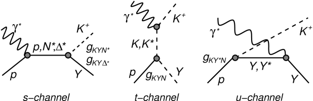
Figure 2: Feynman diagrams representing $s$-channel nucleon ($p,N^{*},\Delta^{*}$) exchange (left), $t$-channel kaon ($K,K^{*}$) exchange (middle), and $u$-channel hyperon ($Y,Y^{*}$) exchange (right) that contribute to the reaction models. The vertex labels $g_{MBB}$ represent the strong coupling constants.

Two different hadrodynamic models are employed in this work. The first is the model of Bennhold and Mart bennhold (referred to here as BM) and the second is model B of Janssen et al. janssen1 (referred to here as JB). In these models, the coupling strengths have been determined mainly by fits to existing $\gamma p\to K^{+}Y$ data (with some older electroproduction data included in some cases) by adding the non-resonant Born terms with a number of resonance terms in the $s$, $t$, and $u$ reaction channels, leaving the coupling constants as free parameters. The coupling constants are required to respect the limits imposed by SU(3) allowing for a symmetry breaking at the level of about 20%. Both models have been compared against the existing photoproduction data from SAPHIR saphir1 ; saphir2 and CLAS mcnabb ; bradford1 and provide a fair description of those results. The model parameters are not based on fits to any CLAS data. The specific resonances included within these calculations are listed in Table 1.

	$K^{+}\Lambda$		$K^{+}\Sigma^{0}$
Resonance	BM	JB	BM	JB
$N^{*}$(1650) ($S_{11}$)	*	*	*	*
$N^{*}$(1710) ($P_{11}$)	*	*	*	*
$N^{*}$(1720) ($P_{13}$)	*	*	*	*
$N^{*}$(1895) ($D_{13}$)	*	*
$\Delta^{*}$(1900) ($S_{31}$)			*	*
$\Delta^{*}$(1910) ($P_{31}$)			*	*
$K^{*}$(892)	*	*	*	*
$K^{*}_{1}$(1270)	*	*	*
$\Lambda^{*}$(1800) ($S_{01}$)		*
$\Lambda^{*}$(1810) ($P_{01}$)		*		*
$\Sigma^{*}$(1880) ($P_{11}$)				*

Table 1: Resonances included in the hadrodynamic Bennhold and Mart model bennhold and the Janssen et al. model janssen1 highlighted in this work for both the $K^{+}\Lambda$ and $K^{+}\Sigma^{0}$ final states.

For $K^{+}\Lambda$ production, the BM model includes the Born terms as well as four baryon resonance contributions. Near threshold, the steep rise of the cross section is accounted for with the $N^{*}$ states $S_{11}$(1650), $P_{11}$(1710), and $P_{13}$(1720). To explain the broad bump in the energy dependence of the cross section seen by SAPHIR saphir1 and CLAS mcnabb ; bradford1 , the BM model includes a spin-3/2 $D_{13}$(1895) resonance that was predicted in the relativized quark model of Capstick and Roberts capstick to have a strong coupling to the $K^{+}\Lambda$ channel, but which was not well established from existing pion-production data. In addition this model includes $t$-channel exchange of the vector $K^{*}$(892) and pseudovector $K_{1}$(1270) mesons. In this model the inclusion of hadronic form factors leads to a breaking of gauge invariance which is restored by the inclusion of counter terms following the prescription of Haberzettl haber .

For $K^{+}\Sigma^{0}$ production, the BM model includes the Born terms as well as the $N^{*}$ resonances $S_{11}$(1650), $P_{11}$(1710), and $P_{13}$(1720), and the $\Delta^{*}$ resonances $S_{31}$(1900) and $P_{31}$(1910). The model also includes $K^{*}$(892) and $K_{1}$(1270) exchanges. The modeling of hadronic form factors for the $\Sigma^{0}$ channel is handled as described above for the $\Lambda$ channel. The BM model does not include any $u$-channel diagrams for either $KY$ final state.

In this work, we also compare our data against model B of Janssen et al. janssen1 , which counterbalances the strength from the Born terms by introducing hyperon resonances in the $u$-channel, where a destructive interference of the $u$-channel hyperon resonance terms with the other background terms occurs. The authors of Ref. janssen1 ; janssen2 claim that this is a plausible way to reduce the Born strength. For the $K^{+}\Lambda$ calculations, the included $u$-channel resonances are the $\Lambda^{*}$ states $S_{01}$(1800) and $P_{01}$(1810). For the $K^{+}\Sigma^{0}$ calculations, the included $u$-channel resonances are the $\Lambda^{*}$ $P_{01}$(1810) and the $\Sigma^{*}$ $P_{11}$(1880). Ref. janssen3 states that there is very little theoretical guidance on how to select the relevant resonances and how to determine realistic values for the associated coupling constants. It is stated that the same qualitative destructive interference effect was observed for other $u$-channel resonance choices, and that the introduced resonances should be interpreted more properly as “effective” particles that account for a larger set of hyperon resonances participating in the process. The $s$-channel and $t$-channel resonances included in the JB model are nearly the same as in the BM model. Hadronic form factors are included in the model with gauge invariance restoration based on the approach by Gross and Riska gross .

Different models have markedly different ingredients and fitted coupling constants. Certainly not every available hadrodynamic model is discussed in this work. However, it is worth mentioning that analysis of Saghai et al. saghai , using the same data set employed for the BM and JB models, have shown that by tuning the background processes involved in the $K^{+}\Lambda$ reaction in the form of additional $u$-channel resonances, the need to include the extra $D_{13}$ $N^{*}$ state was removed. Another analysis including newer photo- and electroproduction data from JLab by Ireland et al. ireland has shown some evidence for the need for an additional $N^{*}$ state at about 1900 MeV (one or more of $S_{11}$, $P_{11}$, $P_{13}$, $D_{13}$), however they concluded that a more comprehensive data set would be required to make further progress.

A recent coupled-channels analysis by Sarantsev et al. sarantsev of the photoproduction data from SAPHIR and CLAS, as well as beam asymmetry data from LEPS for $K^{+}\Lambda$ leps1 and data from $\pi$ and $\eta$ photoproduction, reveals evidence for new baryon resonances in the high $W$ mass region. In this analysis, the full set of data can only be satisfactorily fit by including a new $P_{11}$ state at 1840 MeV and two $D_{13}$ states at 1870 and 2130 MeV. Of course these fits have certain ambiguities that can be resolved or better constrained by incorporating electroproduction data.

The CLAS and SAPHIR photoproduction experiments measured only the $\sigma_{T}$ term. The more recent CLAS data mcnabb ; bradford1 , with higher statistical precision and finer binning compared to the SAPHIR data saphir1 ; saphir2 , reveal that the strength and centroid of the $W$ structure near 1.9 GeV changes with angle, indeed pointing to the possible existence of more than one $s$-channel resonance as suggested by the analysis of Ref. sarantsev . The interference structure functions, $\sigma_{TT}$ and $\sigma_{LT}$, which are accessible in the electroproduction data and presented in this work, will be useful in further constraining and testing models that include new $s$-channel resonance diagrams in this mass region. In addition, the $\sigma_{T}$ and $\sigma_{L}$ structure functions will also provide crucial information to constrain the model parameters for the resonance and background diagrams.

IV.2 Regge Models

In this work we also compare our results to a Reggeon-exchange model from Guidal, Laget, and Vanderhaeghen guidal (referred to here as the GLV model). This calculation includes no baryon resonance terms at all, but is instead based only on gauge invariant $t$-channel $K$ and $K^{*}$ Regge trajectory exchange. It therefore provides a complementary basis for studying the underlying dynamics of strangeness production. It is important to note that the Regge approach has far fewer parameters compared to the hadrodynamic models. These include the $K$ and $K^{*}$ form factors, which in the GLV model are assumed to be of a monopole form $F_{K,K^{*}}=[1+Q^{2}/\Lambda_{K,K^{*}}^{2}]^{-1}$ with a mass scale $\Lambda_{K,K^{*}}$=1.5 GeV² chosen to reproduce the JLab Hall C $\sigma_{L}$, $\sigma_{T}$ data mohring . In addition, the model employs values for the coupling constants $g_{KYN}$ and $g_{K^{*}YN}$ taken from photoproduction studies.

The model was fit to higher-energy photoproduction data where there is little doubt of the dominance of these kaon exchanges, and extrapolated down to JLab energies. An important feature of this model is the way gauge invariance is achieved for the kaon $t$-channel exchange by Reggeizing the $s$-channel nucleon pole contribution in the same manner as the kaon $t$-channel diagram guidal1 . This approach has been noted as a possible reason why the Regge model, despite not including any $s$-channel resonances, was able to reproduce the JLab Hall C $\sigma_{L}/\sigma_{T}$ data at $Q^{2}\geq 0.5$ GeV². The stated reason is that due to gauge invariance, the $t$-channel kaon exchange and $s$-channel nucleon pole terms are inseparable and must be treated on the same footing. In the GLV Regge model these terms are Reggeized in the same way and multiplied by the same electromagnetic form factor. No counter terms need to be introduced to restore gauge invariance as is done in the hadrodynamic approach guidal .

V Experiment Description and Data Analysis

The experiment was performed using the electron beam at JLab and the CLAS detector in Hall B. An electron beam of 5 nA current was incident upon a 5-cm long liquid-hydrogen target, resulting in an average beam-target luminosity of $\mathcal{L}\approx 10^{34}~{}\mathrm{cm^{-2}s^{-1}}$. Data were taken with beam energies of 2.567, 4.056, and 4.247 GeV. In this analysis the 4.056 and 4.247 GeV data have been combined into a single data set, referred to throughout this work as the 4 GeV data set. The 2.567 data set has a live-time corrected luminosity of about 1.32 fb^-1, while that for the 4.056 and 4.247 GeV data sets are about 0.67 fb^-1 and 0.80 fb^-1, respectively. The beam was effectively continuous with a 2.004 ns bunch structure. The large acceptance of CLAS enabled us to detect the final state electron and kaon over a broad range of momentum transfer $Q^{2}$ and invariant energy $W$ as shown in Fig. 3.

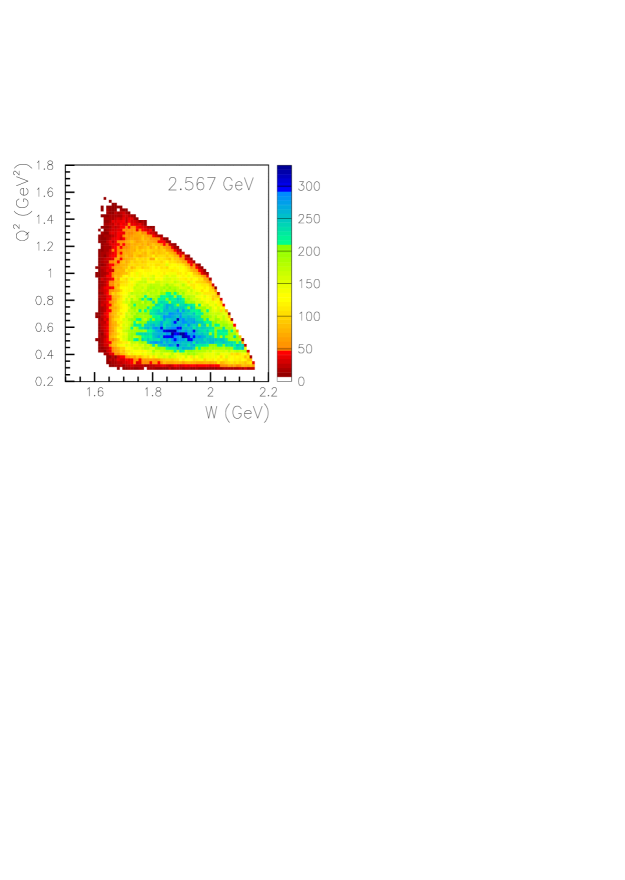
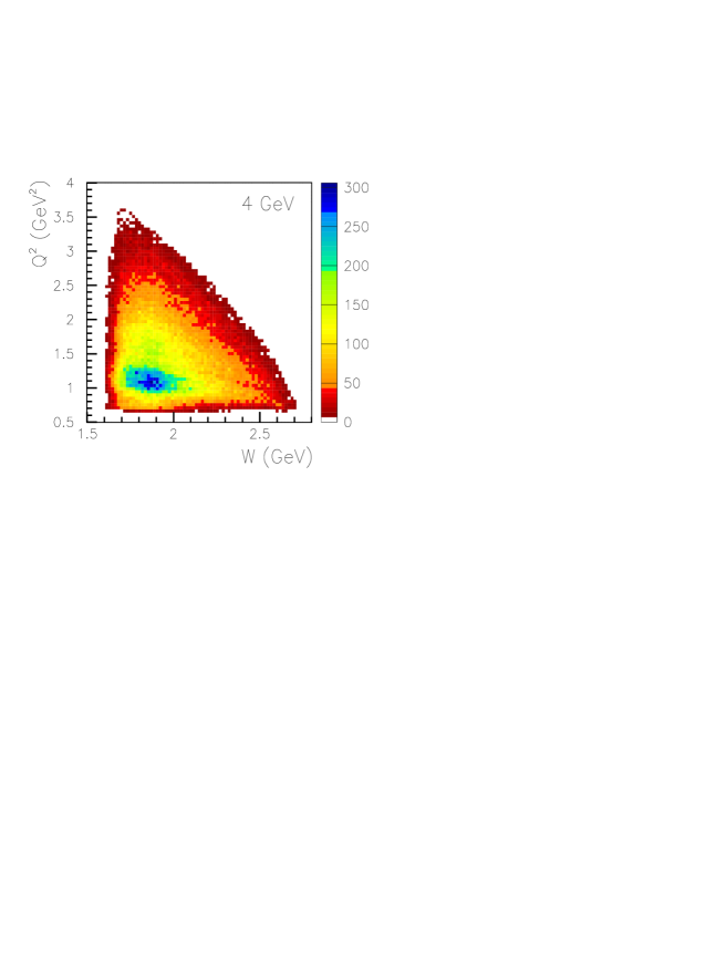
Figure 3: (Color online) CLAS kinematic coverage in terms of $Q^{2}$ vs. $W$ for $p(e,e^{\prime}K^{+})Y$ ($Y=\Lambda,\Sigma^{0}$) events for beam energies of 2.567 GeV (left) and 4 GeV (right).

CLAS is a large-acceptance detector clas used to detect multi-particle final states from reactions initiated by either real photon or electron beams. The central element of the detector is a six-coil superconducting toroidal magnet that provides a mostly azimuthal magnetic field, with a field-free region surrounding the target. The integrated field strength varies from 2 T$\cdot$m for high momentum tracks at the most forward angles to about 0.5 T$\cdot$m for tracks beyond 90^∘. The field polarity was set to bend negatively charged particles toward the electron beam line. Drift chambers (DC) situated before, within, and outside of the magnetic field volume provide charged-particle tracking with a momentum resolution of 1-2% depending upon the polar angle within the six independent sectors of the magnet dcnim . To protect the chambers from the charged electromagnetic background emerging from the target, a small normal-conducting “mini-torus” magnet was located just outside the target region. The integral magnetic field of the mini-torus is about 5% that of the main torus.

The outer detector packages of CLAS that surround the magnet and drift chambers consist of large-volume gas Čerenkov counters (CC) for electron identification ccnim , scintillators (SC) for triggering and charged particle identification via time-of-flight scnim , and a lead-scintillator electromagnetic shower counter (EC) used for electron/pion separation as well as neutral particle detection and identification ecnim . An open trigger for scattered electrons formed from a coincidence of the CC and EC signals within a given sector gave event rates of about 2 kHz. The total beam charge was integrated with a Faraday cup to an accuracy of better than 1%.

The offline event reconstruction first identified a viable electron candidate by matching a negatively charged track in the DC with hits in the SC, CC, and EC counters. The hits in the CC and EC counters were required to be within a fiducial region where the efficiency was large and uniform. The track was projected to the target vertex to estimate the event start time; the estimate was compared to the phase of the accelerator radio-frequency (RF) signal to determine this time to better than 50 ps ($\sigma$). In contrast to a straightforward subtraction of the electron start time from the $K^{+}$ time, this use of the highly stable RF phase improved the hadronic time-of-flight measurements by almost a factor of $\sqrt{2}$.

A positively charged kaon candidate was identified as an out-bending track found in the DC that spatially matched to a SC hit that projected back to the target. The measured time-of-flight of the track and the fitted path length were used to calculate the velocity of the particle. This velocity and the measured momentum were used to calculate the mass of each charged hadron. For the data discussed here, the kaon momentum range was between 300 MeV (software cut) and $\approx$3 GeV (kinematic limit), with a typical flight path of 4.5 m. The measured mass resolution was primarily due to the reconstructed time-of-flight resolution, which was 190 ps ($\sigma$) on average, and also included contributions from the 1.5% momentum resolution and 0.5 cm path-length uncertainty. A loose cut around the reconstructed kaon mass was used to initially select the kaon candidates (a data filtering condition), however a large background of positively charged pions and protons still remained. A momentum-dependent mass cut was used to select the $K^{+}$ events for the final analysis as shown in Fig. 4 for our filtered data files.

Figure 4: (Color online) Reconstructed mass for positively charged particles. The left figure shows the mass plotted against the measured momentum. The lines show the mass cuts used to identify kaon candidates. A logarithmic yield density scale is employed. The right figure shows the reconstructed mass. These spectra were made from our kaon-filtered data files.

Corrections to the electron and kaon momenta were devised to correct for reconstruction inaccuracies. These arise due to relative misalignments of the drift chambers in the CLAS magnetic field, as well as for uncertainties in the magnetic field map employed during charged track reconstructions. These corrections were typically less than 1%.

Using the four-momenta of the incident electron, scattered electron, and $K^{+}$ candidate, the missing mass, corresponding to the mass of the recoiling hyperon, was calculated. The missing-mass distribution contains a background that includes a continuum beneath the hyperons that arises due to multi-particle final states where the candidate $K^{+}$ results from a misidentified pion or proton, as well as events from $ep$ elastic scattering (protons misidentified as kaons) and events from $\pi^{+}n$ final states (pions misidentified as kaons). The elastic events are kinematically correlated and show up clearly in plots of $\theta_{K}^{*}$ (c.m. angle) versus missing mass and $\theta_{K}$ (lab angle) versus $Q^{2}$ (Figs. 5a and b, respectively). A cut on the elastic band in the $\theta_{K}$ versus $Q^{2}$ space removes this contribution with a small loss of hyperon yield that is later accounted for with our Monte Carlo generated acceptance function. The $\pi^{+}n$ events are removed with a simple missing-mass cut in which the detected kaon candidates are assumed to be pions. Typical missing-mass distributions showing clear $\Lambda(1116)$ and $\Sigma^{0}(1193)$ peaks are shown in Fig. 6.

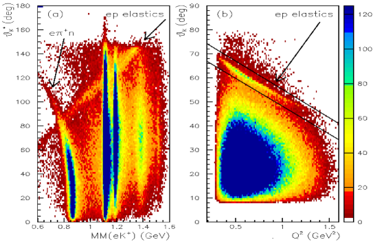
Figure 5: (Color online) (a) $\theta_{K}^{*}$ versus $p(e,e^{\prime}K^{+})Y$ missing mass showing $ep$ elastic events and $e\pi^{+}n$ events. The vertical bands correspond to ground state $\Lambda(1116)$, $\Sigma^{0}(1193)$, and $\Lambda(1405)/\Sigma^{0}(1385)$ hyperons. (b) $\theta_{K}$ versus $Q^{2}$ for $p(e,e^{\prime}K^{+})Y$ showing the $ep$ elastic events and the cut used to remove them.

The continuum from the multi-particle final states that lies beneath the $\Lambda$ and $\Sigma^{0}$ hyperon peaks in our mass spectra is accounted for by a fitting process in which identified pions and protons in our unfiltered data files are assumed to be kaons. Missing-mass distributions are generated for each assumption in each of our different bins in $Q^{2}$, $W$, $\cos\theta_{K}^{*}$, and $\Phi$. The resulting distributions, along with template shapes for the $\Lambda$ and $\Sigma^{0}$ hyperons determined from Monte Carlo simulations, are fit to the missing-mass spectra using a maximum-log-likelihood method appropriate for the low statistical samples in our four-dimensional bins. The template shapes for the hyperons were produced from a simulation that included radiative processes and was matched to the detector resolution. Typical fits of the missing-mass distributions are shown in Fig. 6. The final yields in each kinematic bin were determined by taking the number of counts determined from the fits that fell within a mass window around the $\Lambda$ (1.095 to 1.165 GeV) and $\Sigma^{0}$ (1.165 to 2.3 GeV) peaks. Hyperon events in the tails of the distributions that fell outside of our mass windows were accounted for by our acceptance correction function. After removal of all backgrounds, a total of $1.4\times 10^{5}$ $K^{+}\Lambda$ and $6.7\times 10^{4}$ $K^{+}\Sigma^{0}$ final state events were obtained across the entire kinematic range for the 2.567 GeV data set, while $9.7\times 10^{4}$ $K^{+}\Lambda$ and $4.7\times 10^{4}$ $K^{+}\Sigma^{0}$ events were obtained for the 4 GeV data set.

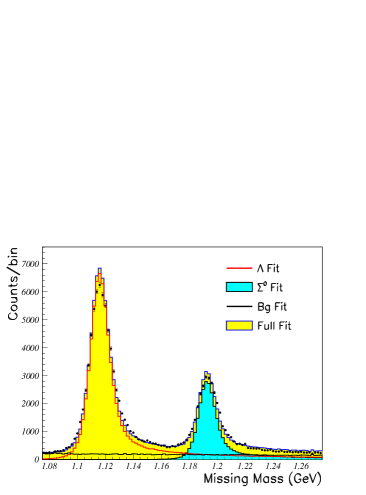
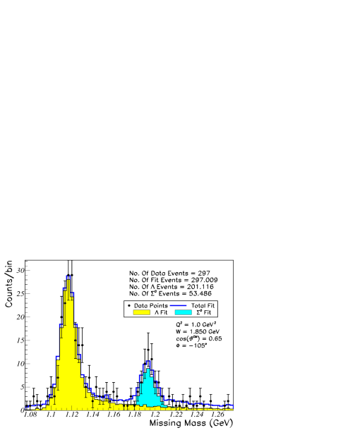
Figure 6: (Color online) Signal and background fits from the 2.567 GeV data for the $e^{\prime}K^{+}$ missing mass spectrum summed over all kinematics (left) and for a typical $\cos\theta_{K}^{*}$/$\Phi$ bin (right) at $Q^{2}$=1.0 GeV² and $W$=1.85 GeV to demonstrate the typical fit quality in our data.

	2.567 GeV				4 GeV
Variable	Nbins	Range	Nbins	Range	Nbins	Range
$Q^{2}$	2	0.5 – 0.8			4	0.9 – 1.3
(GeV2)		0.8 – 1.3				1.3 – 1.8
						1.8 – 2.3
						2.3 – 2.8
$W$	8	1.60 – 1.70	5	1.60 – 1.70	8	1.6 – 1.7
(GeV)		1.70 – 1.75		1.70 – 1.80		1.7 – 1.8
		1.75 – 1.80		1.80 – 1.90		1.8 – 1.9
		1.80 – 1.85		1.90 – 2.00		1.9 – 2.0
		1.85 – 1.90		2.00 – 2.10		2.0 – 2.1
		1.90 – 1.95				2.1 – 2.2
		1.95 – 2.00				2.2 – 2.3
		2.00 – 2.10				2.3 – 2.4
$\cos\theta_{K}^{*}$	6	-0.8 – -0.4			6	-0.8 – -0.4
		-0.4 – -0.1				-0.4 – -0.1
		-0.1 – 0.2				-0.1 – 0.2
		0.2 – 0.5				0.2 – 0.5
		0.5 – 0.8				0.5 – 0.8
		0.8 – 1.0				0.8 – 1.0
$\Phi$	8	$\cos\theta_{K}^{*}<-0.1$			8	$\cos\theta_{K}^{*}<0.2$
	12	$\cos\theta_{K}^{*}>-0.1$			12	$\cos\theta_{K}^{*}>0.2$

Table 2: The number of bins and the bin sizes employed for the 2.567 and 4 GeV analyses in this work. For the 2.567 GeV data analysis two different binning choices were made for $W$ for each bin in $Q^{2}$, $\cos\theta_{K}^{*}$, and $\Phi$.

The data were binned in a four-dimensional space of the independent kinematic variables, $Q^{2}$, $W$, $\cos\theta_{K}^{*}$, and $\Phi$. Table 2 lists the kinematic bin definitions used in the analysis. The data at 2.567 GeV consisted of data sets taken with two settings of the main CLAS torus field that were combined together. As mentioned above, our 4 GeV data set consisted of data acquired at beam energies of 4.056 and 4.247 GeV at the same torus field setting. When combining the data at 4.056 and 4.247 GeV, we evolve the cross sections at 4.247 GeV to the bin center of the 4.056 GeV data using our model of the cross section. As the two data sets are close in energy and $\epsilon$, there is little systematic uncertainty involved in this procedure.

In this analysis the number of $\Phi$ bins was 8 for the two backward-most bins of $\theta_{K}^{*}$ and 12 for the four forward-most $\theta_{K}^{*}$ bins. The larger number of $\Phi$ bins for forward and central $\theta_{K}^{*}$ increased the reliability of the $\Phi$-fits in the presence of the forward beam “hole” of the spectrometer, an area of depleted acceptance corresponding to tracks with small laboratory angles. Bins significantly overlapping this forward hole were excluded from our analysis.

The average differential cross section for each hyperon final state in each bin $i$ was computed using the form:

$$\frac{d\sigma_{v}^{i}}{d\Omega_{K}^{*}}=\frac{1}{\Gamma_{v}}\left(\frac{1}{\Delta Q^{2}\Delta W\Delta\cos\theta^{*}_{K}\Delta\Phi}\right)\left(\frac{N_{i}}{R_{i}A_{i}}\right)\left(\frac{1}{N_{0}(N_{A}\rho t/A_{w})}\right),$$ (6)

where $N_{i}$ is the hyperon yield, $A_{i}$ is the acceptance, $N_{0}$ is the live-time corrected incident electron flux, $R_{i}$ is the radiative correction factor, $N_{A}$ is Avogadro’s number, $\rho$ is the target density ($\langle\rho\rangle$ = 0.072 g/cm³), $t$ is the target length, and $A_{w}$ is the atomic weight of hydrogen (1.00794 g/mol). The product $\Delta Q^{2}\Delta W\Delta\cos\theta^{*}_{K}\Delta\Phi$ represents the volume of the $i^{th}$ bin corrected for kinematic limits.

The geometric acceptance and reconstruction efficiencies were calculated using a standard model of the CLAS detector based upon a GEANT simulation geant . To reduce the model dependence of the computed CLAS acceptance, it is important to match the distributions of accepted data and Monte Carlo events as a function of the relevant kinematic variables $Q^{2}$, $W$, $\cos\theta_{K}^{*}$, and $\Phi$ for both the $K^{+}\Lambda$ and $K^{+}\Sigma^{0}$ final states. This match must be ensured at all beam energies and torus field settings employed in the analysis.

A variety of reaction models (see e.g. Ref. bennhold ) were employed as input event generators for the simulated events. Because none of the models agreed particularly well with our $K^{+}\Lambda$ or $K^{+}\Sigma^{0}$ data, we developed our own models that were able to match the data reasonably well over our full kinematic phase space. We developed two different ad hoc models for the $K^{+}\Lambda$ analysis that both represented our data equally well, although with slightly different dependencies on $Q^{2}$, $W$, and $\cos\theta_{K}^{*}$. One ad hoc model was developed for the $K^{+}\Sigma^{0}$ analysis. These models were used as input to determine our detector acceptance function, radiative corrections, and bin-centering correction factors. In addition we developed an event generator based on fits to our $K^{+}\Lambda$ data. Differences between our two ad hoc models and our data-fitted model for $K^{+}\Lambda$ were used to estimate the model dependence of our results. Further details are included in Section VII. Figure 7 shows the dependence of the $K^{+}\Lambda$ acceptance upon $\theta_{K}^{*}$ and $\Phi$ for a bin in $Q^{2}$ and $W$. Typical acceptances of CLAS for the $e^{\prime}K^{+}$ final state were in the range of 1 to 30% depending on kinematics. Note the strong variation in acceptance as a function of both $\cos\theta_{K}^{*}$ and $\Phi$ due to the geometry of CLAS.

Figure 7: Distribution of the computed $K^{+}\Lambda$ acceptance for CLAS as a function of $\cos\theta_{K}^{*}$ and $\Phi$ for the $W$=1.85 GeV and $Q^{2}$=0.65 GeV² bin. The depleted area near $\Phi$ of $0^{\circ}$ for forward angles is the forward “hole” in CLAS due to the beam pipe. The number of bins in $\Phi$ is different for forward and backward $\cos\theta_{K}^{*}$. The statistical error bars from the Monte Carlo are smaller than the symbol size on this plot. The curves on each plot serve only to guide the eye.

In the detector simulation, particles generated at the target were propagated through the CLAS magnetic field and were permitted to interact with materials and to undergo decay. These tracks then generated simulated detector hits. Hits corresponding to the known dead areas in the detectors were removed, and the hits were smeared according to the known detector resolution effects. These simulated events were passed through the same analysis chain as the real data. Geometrical fiducial cuts were applied to both the data and simulated events to eliminate areas of inefficient detector response or where the response was not well modeled. These areas were typically within a few degrees of the magnet coils and near the edges of the Čerenkov detector.

The radiative correction for each kinematic bin was computed from the ratio of the model cross sections with and without radiative effects. We used two very different methods to compute this correction factor.

The first method used an acceptance-rejection technique, where events were generated uniformly in $W$, $Q^{2}$, $\cos\theta^{*}_{K}$, and $\Phi$, with a weight determined via the cross section model of Ref. bennhold . The energies of externally radiated photons from the incident electron, and from the emitted electron and kaon in the region of the target proton, were generated according to the formulas of Mo and Tsai motsai . The weight of the event was adjusted to account for hard and soft internal radiative effects, and the post-radiation kinematic variables were calculated to identify the bin into which the event fell. While lacking in computational efficiency, this method benefited from being able to compute cross sections as well as the expected event distributions, both with and without radiative effects, thus providing a consistent event sample to use for the acceptance studies. The second method used the same formula for calculating the radiated cross section from the assumed non-radiated model. However, it integrated the resulting six-dimensional cross section over the two unseen dimensions that corresponded to a radiated photon from either the initial or scattered electron. The ratio of the integrated radiated cross section (now corresponding to a four-dimensional space) to the unradiated cross section yielded the radiative correction factor. We chose to use this second method because of its superior computational speed. It was extensively checked versus the “EXCLURAD” code of Afanasev afanasev . Differences between the two methods allowed us to estimate the size of any residual uncertainty in the radiative correction procedure (see Section VII).

In order to do a full separation into four structure functions, we can fit our full set of data including the differential cross sections from both beam energies with a function of the form $f(\Phi,\epsilon)$; the fitted parameters being the values of $\sigma_{T}$, $\sigma_{L}$, $\sigma_{TT}$, and $\sigma_{LT}$ at some fixed point in $Q^{2}$, $W$, and $\cos\theta_{K}^{*}$. Alternatively, we can extract $\sigma_{U}$ in each $Q^{2}$, $W$, and $\cos\theta_{K}^{*}$ bin from a $\Phi$ fit for each beam energy separately, and then do a linear $\epsilon$ fit to separately extract $\sigma_{T}$ and $\sigma_{L}$; this being the well-known Rosenbluth separation technique. In either case, in order to do these fits, we must first define the cross sections at a specific fixed point within the bin, and not merely as an average over a given bin volume. This is especially true when the bins are large and event-weighted average values of kinematic variables can be different for different $\Phi$ bins. Using an integration over our model cross section, we calculate the cross section at the fixed point given its average over the bin volume. This correction is referred to as a “bin-centering correction”, or more accurately, as a “finite bin size correction”. By using our model event generators, we simply calculated the ratio of the cross section evaluated at the assigned bin center to the average cross section integrated over the bin to obtain the finite bin size correction factor. Systematic uncertainties associated with these corrections were extensively studied (see Section VII).

In Fig. 8 we show a sample of the $\Phi$-dependent differential cross sections for the $K^{+}\Lambda$ final state at representative kinematic points. The different shapes of the differential cross sections vs. $\Phi$ in each of our bins in $Q^{2}$, $W$, and $\cos\theta_{K}^{*}$ reflect differences of the interference terms, $\sigma_{TT}$ and $\sigma_{LT}$. The differences in scale reflect the differences in $\sigma_{U}$.

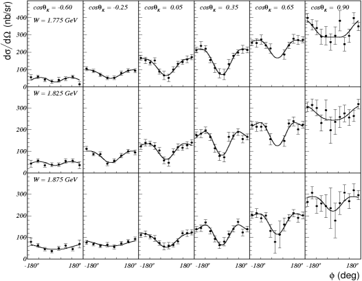
Figure 8: $\Phi$-dependent differential cross sections (nb/sr) and fits for $K^{+}\Lambda$ events from our 2.567 GeV data at $Q^{2}$=0.65 GeV² for each of our six $\cos\theta_{K}^{*}$ bins (labeled at the top of each column) for three different $W$ bins (labeled on the left of each row). The curves represent fits to the $\Phi$-dependent differential cross sections.

VI Structure Function Extraction

The full set of differential cross sections $d\sigma_{v}/d\Omega_{K}^{*}$ included in this work for each hyperon final state consists of 156 bins in $Q^{2}$, $W$, and $\cos\theta_{K}^{*}$ for the 2.567 GeV data (accounting for both $W$ binning scenarios given in Table 2) and 192 bins for the 4 GeV data. This amounts to 1664 data points in $Q^{2}$, $W$, $\cos\theta_{K}^{*}$, and $\Phi$ for the 2.567 GeV data and 1920 data points at 4 GeV for each hyperon final state. In this section we provide details regarding the structure function extraction. In Section VI.1 we focus on the separation of the structure functions $\sigma_{U}$, $\sigma_{TT}$, and $\sigma_{LT}$. In Section VI.2 we present the extraction of $\sigma_{T}$ and $\sigma_{L}$ separately from $\sigma_{U}$ using a Rosenbluth fit and also a simultaneous $\epsilon-\Phi$ fit of our data at 2.567 and 4 GeV.

VI.1 Extraction of $\sigma_{U}$, $\sigma_{TT}$, and $\sigma_{LT}$

The differential cross sections plotted in Fig. 8 are actually the mean values within the finite size of the $\Phi$ bins and therefore do not necessarily reflect the value at the bin center. Thus directly fitting these data with eq.(5) to extract the structure functions $\sigma_{U}=\sigma_{T}+\epsilon\sigma_{L}$, $\sigma_{TT}$, and $\sigma_{LT}$ would be inappropriate. Integrating eq.(5) over the finite bin size, $\Delta\Phi=\Phi_{u}-\Phi_{l}$, where $\Phi_{u}$ and $\Phi_{l}$ are the upper and lower limits of the bin, respectively, gives:

$$\bar{\sigma}_{0} \equiv \frac{1}{\Delta\Phi}\int_{\Phi_{l}}^{\Phi_{u}}\left(\sigma_{U}+\epsilon\sigma_{TT}\cos 2\Phi+\sqrt{\epsilon(\epsilon+1)}\sigma_{LT}\cos\Phi\right)d\Phi$$ (7)

$$= \frac{1}{\Delta\Phi}\left(\sigma_{U}\Delta\Phi+\frac{\epsilon}{2}\sigma_{TT}\left(\sin 2\Phi_{u}-\sin 2\Phi_{l}\right)+\sqrt{\epsilon(\epsilon+1)}\sigma_{LT}\left(\sin\Phi_{u}-\sin\Phi_{l}\right)\right).$$

$\bar{\sigma}_{0}$ now represents the value of the measured bin-averaged cross section in a given $\Phi$ bin and fitting the data with eq.(7) yields the separated structure functions for a given bin in $Q^{2}$, $W$, and $\cos\theta_{K}^{*}$. The “$\epsilon$” pre-factors were evaluated at the bin center and divided out.

Prior to the $\Phi$ fits, the statistical uncertainty of each cross section bin was combined linearly with that portion of the systematic uncertainty arising from the yield extraction procedures (see Section VII for details). A few points were removed from the fits based upon their low acceptance in CLAS, in order to prevent bins with a very small acceptance from distorting the extracted structure functions. A point was rejected if its acceptance at 2.567 GeV (4 GeV) was less than 2.0% (1.0%) or less than 10.0% (5.0%) of the average acceptance over all bins at the same $Q^{2}$, $W$, and $\cos\theta_{K}^{*}$.

In reporting the final results from our $\Phi$ fits, several $\cos\theta_{K}^{*}$ bins have been discarded. In general, these bins were near the edge of our kinematic acceptance and had limited $\Phi$ coverage. In addition, the statistical uncertainties were large on the points in these bins that survived the acceptance criteria described above. Typically, the missing points were near $\Phi=\pm\pi$ or $\Phi=0$ – exactly where points are needed to constrain the interference structure functions. The resulting $\Phi$ fits for these bins had $\chi^{2}/\nu$ values, where $\nu$ represents the number of degrees of freedom, that were uniformly too small considering the expected $\chi^{2}/\nu$ distributions. In other words, a three-parameter fit of these bins had too many parameters, given the low number of data points and the large uncertainties, to give unambiguous solutions for the structure functions. We also examined the $\chi^{2}/\nu$ distributions for the remaining fits and found that they were well represented by their expected probability distributions, which instills confidence in the quality of the data, the assigned uncertainties, and the fits.

VI.2 Separation of $\sigma_{T}$ and $\sigma_{L}$

The extraction procedure detailed in Section VI.1 yielded the bin-centered structure functions $\sigma_{U}$, $\sigma_{TT}$, and $\sigma_{LT}$. To further separate $\sigma_{U}$ into its component parts, $\sigma_{T}$ and $\sigma_{L}$, we have two options. The first is the standard Rosenbluth separation technique, in which $\sigma_{U}$ is determined for two different beam energies (or different $\epsilon$ values) but for the same point in $Q^{2}$, $W$, and $\cos\theta_{K}^{*}$, and fit as a linear function of $\epsilon$. An alternative approach is to simultaneously fit the data from the two energies as a function of $\epsilon$ and $\Phi$, this time explicitly replacing $\sigma_{U}$ in eq.(7) with $\sigma_{T}+\epsilon\sigma_{L}$. This method has the advantage of constraining the individual parameters, $\sigma_{T}$, $\sigma_{L}$, $\sigma_{TT}$, and $\sigma_{LT}$ to have the same value for the two different beam energies, as they must since they are explicit functions of $Q^{2}$, $W$, and $\theta_{K}^{*}$ only. This approach represents an important systematic check as the forward beam hole of CLAS affects the acceptance function differently at 2.567 GeV relative to 4.056 and 4.247 GeV.

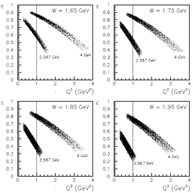
Figure 9: CLAS acceptance of the scattered electron in terms of $\epsilon$ vs. $Q^{2}$ at 2.567 GeV (lower bands) and 4 GeV (upper bands) for four 100-MeV $W$ bins centered from 1.65 to 1.95 GeV. The vertical line at $Q^{2}$=1.0 GeV² marks where we have performed the separation of $\sigma_{T}$ and $\sigma_{L}$.

The separation of the structure functions $\sigma_{T}$ and $\sigma_{L}$ can only be performed in ($Q^{2}$, $W$, $\cos\theta_{K}^{*}$) bins where the 2.567 GeV and 4 GeV data overlap. Figure 9 shows plots of $\epsilon$ vs. $Q^{2}$ for four different 100-MeV wide bins in $W$ from 1.65 GeV to 1.95 GeV, and highlights the kinematic coverage of CLAS. The cut-off at low $Q^{2}$ is due to the minimum $\theta_{e}$ detectable by CLAS and the low $\epsilon$ cut-off is due to the maximum $\theta_{e}$ detectable by the Čerenkov detectors. For this analysis, the data overlap only for a rather narrow $Q^{2}$ region at about 1 GeV². We have performed a separation of $\sigma_{T}$ and $\sigma_{L}$ for $Q^{2}$=1.0 GeV² for the $K^{+}\Lambda$ final state for $W$=1.65, 1.75, 1.85, and 1.95 GeV, and at values of $W$=1.75, 1.85, and 1.95 GeV for the $K^{+}\Sigma^{0}$ final state. In this two beam energy separation, we have typical differences in $\epsilon$ of about 0.4. Of central importance in this analysis is the fact that this separation is performed for the first time away from the condition of parallel kinematics (i.e. $\theta_{K}^{*}$=0^∘ or along the virtual photon direction).

Before the separation of $\sigma_{U}$ could proceed, we first had to account for the binning differences between the 2.567 GeV and 4 GeV data sets. Due to consideration of statistics in the two separate data sets, the 2.567 GeV data were sorted in 50-MeV wide $W$ bins for the extraction of $\sigma_{U}$, $\sigma_{TT}$, and $\sigma_{LT}$, while the data at 4 GeV were sorted in 100-MeV wide $W$ bins (see Table 2). In order to perform either the Rosenbluth fit or the simultaneous $\epsilon-\Phi$ fit, the 2.567 GeV data had to be resorted into $W$ bins that were 100-MeV wide. In computing the cross sections for the 100-MeV wide $W$ bins at 2.567 GeV, the hyperon yield fits were redone and all other factors associated with computing the cross section were recalculated using Monte Carlo based on the 100-MeV wide bin.

The Rosenbluth extraction procedure is a standard technique to separate $\sigma_{T}$ and $\sigma_{L}$. The error bars on these structure functions result from the statistical and systematic uncertainties on the two $\sigma_{U}$ cross section points used in the extraction. With only two data points, the slope parameter ($\sigma_{L}$) and the intercept parameter ($\sigma_{T}$) along with their associated uncertainties, can be computed analytically. Figure 10 shows a representative plot of the $\sigma_{U}$ cross sections for the $K^{+}\Lambda$ final state at $W$=1.85 GeV for each of our six $\cos\theta_{K}^{*}$ bins. This plot also serves to indicate the typical $\epsilon$ values and spread for the two data sets. The data points at 2.567 GeV and 4 GeV have each been evolved using our ad hoc models to the point $Q^{2}$=1.0 GeV². The analysis employs the highest $Q^{2}$ bin from our 2.567 GeV data set and the lowest $Q^{2}$ bin from our 4 GeV data set.

Figure 10: Representative Rosenbluth separation plots of $\sigma_{U}$ (nb/sr) vs. $\epsilon$ for our $K^{+}\Lambda$ data at $Q^{2}$=1.0 GeV² and $W$=1.85 GeV for our six $\cos\theta_{K}^{*}$ bins. The lines represent the fits that determine the slope parameter ($\sigma_{L}$) and the intercept parameter ($\sigma_{T}$), which are printed on each plot. The error bars on the data points and the errors listed for $\sigma_{L}$ and $\sigma_{T}$ on each plot represent the combined statistical and systematic uncertainties.

An example of the comparison between the separate $\Phi$ fits for the 2.567 GeV and 4 GeV data and the simultaneous fit for both energies for the $K^{+}\Lambda$ and $K^{+}\Sigma^{0}$ reactions is shown in Fig. 11 for $Q^{2}$=1.0 GeV² and $W$=1.85 GeV. The differences between the differential cross sections for the 2.567 and 4 GeV data for a given bin (see Fig. 11) in $\cos\theta_{K}^{*}$ are due not only to the beam energy dependent $\epsilon$ pre-factors (defined in eq.(5)), but also to the different systematic variations associated with the acceptance functions of CLAS at these energies. Of importance is that the simultaneous fits differ from the single beam energy fits only where the single beam energy fits have large error bars (e.g. 4 GeV back-angle $K^{+}\Sigma^{0}$ bin) or are missing $\Phi$ points due to our minimum acceptance cut-off criteria (e.g. 4 GeV back-angle $K^{+}\Lambda$ bin). In these cases the simultaneous fit procedure leads to extracted structure function with reduced uncertainties compared to the single beam energy fits.

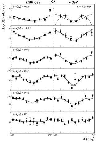
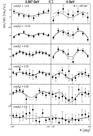
Figure 11: Comparison of $\Phi$ fits to the differential cross sections performed for two different algorithms. In the first approach (dashed curves) the cross sections at 2.567 and 4 GeV are fit separately. In the second approach (solid curves) the two different beam energy data sets are fit simultaneously. These plots are for kinematics with $Q^{2}$=1.0 GeV² and $W$=1.85 GeV for the $K^{+}\Lambda$ (left columns) and $K^{+}\Sigma^{0}$ (right columns) final states at different values of $\cos\theta_{K}^{*}$ as indicated.

VII Systematic Uncertainties

VII.1 Overview

To obtain a virtual photoabsorption cross section, we reconstruct events with an outgoing electron and $K^{+}$, and then fit the missing-mass spectra for each of our bins in $Q^{2}$, $W$, $\cos\theta_{K}^{*}$, and $\Phi$ to obtain the yields for the reactions $K^{+}\Lambda$ and $K^{+}\Sigma^{0}$. The yields are corrected for the acceptance function of CLAS, radiative corrections, and finite bin size effects. Finally, we divide by the virtual photon flux factor at the bin center, the bin volume corrected for kinematic limits, and the beam-target luminosity to yield the cross section. Each of these procedures is subject to systematic uncertainty. We typically estimate the size of systematic uncertainties by repeating a procedure in a slightly different way (e.g. by varying a cut parameter within reasonable limits or by employing a slightly different algorithm) and noting how the results change. The difference in the results is then used as a measure of the systematic uncertainty. In this section we describe our main sources of systematics.

With respect to their effect on our results, there are three types of systematic effects: uncertainties that affect the yield extraction in a seemingly random fashion where the systematic uncertainty is proportional to the size of the statistical uncertainty, “scaling” uncertainties that affect both the cross sections and structure functions by a simple scale factor, and $\Phi$-dependent uncertainties such as using an event generator with a $\Phi$-dependence that does not quite match the data.

These uncertainties are handled in different ways. Because the size of the “yield extraction” uncertainty depends on the size of the statistical uncertainty, we take the random-type systematic uncertainties into account by enlarging the statistical uncertainty before the $\Phi$ fit to extract the structure functions. These fractional systematic scaling uncertainties are multiplied by the value of the cross section or the structure function in question to get the absolute uncertainty. The remaining uncertainties, which can in general have $\Phi$ or other kinematic dependencies, are estimated by extracting the $\Phi$-dependent structure functions for two, similar procedures. This method gives an absolute estimate for a structure function uncertainty.

The primary sources of systematic uncertainty for this experiment came from the Monte Carlo model dependence (acceptance, radiative corrections, finite bin size corrections), detector efficiency, and the yield extraction. With the very large acceptance and a four-dimensional kinematic space, systematic uncertainties were studied on a bin-by-bin basis. Table 3 summarizes our estimates of the average systematic uncertainties on the differential cross sections associated with various effects. The different types of systematic uncertainties mentioned above are referred to as “stat.”, “scaling”, and “$\Phi$-dep.” in the column labeled “Type” in Table 3.

Category	Type	Sources	Avg. Size
i). Event Reconstruction	scaling	Trigger+tracking efficiency	1%
	$\Phi$-dep.	Electron fiducial cut	3.6%
	$\Phi$-dep.	Kaon fiducial cut	4.1%
	scaling	Electron PID efficiency	1.5%
	scaling	Kaon PID efficiency	1.0%
	scaling	CC efficiency	2-5%
	scaling	CLAS forward angle response	1-10%
ii). Yield Extraction	stat.	Signal templates	25% $\cdot$ stat
		Background removal
iii). Model Dependence	$\Phi$-dep.	Acceptance calculations,	8.0%
		Radiative corrections, &
		Finite bin size corrections
iv). RadCorr: Theory	scaling	Integration vs. EXCLURAD	3.4%
v). Photon Flux-factor	scaling	Momentum and angle uncertainties	3.0%
vi). Luminosity	scaling	Live time correction	0.5%
	scaling	Faraday cup accuracy	1.0%
	scaling	Hydrogen target thickness	3.0%

Table 3: Sources, types, and average sizes of systematic uncertainties on the differential cross sections.

The main categories of systematic uncertainty in this analysis include: (i). event reconstruction efficiency ($\delta\sigma_{ER}$), (ii). yield extraction ($\delta\sigma_{YE}$), (iii). model dependence ($\delta\sigma_{MOD}$), (iv). radiative correction theory uncertainty ($\delta\sigma_{RC}$), (v). virtual photon flux ($\delta\sigma_{flux}$), and (vi). luminosity ($\delta\sigma_{\cal{L}}$). Each of these categories is explained in more detail in the next section. The final systematic uncertainty assignment to our extracted structure functions is explained fully in Section VII.3. While the yield extraction systematic uncertainty, as explained below, is treated as an effective increase in our statistical uncertainty, the remaining systematic sources are added in quadrature to arrive at our final uncertainty assignment as:

$$\delta\sigma_{sys}=\left(\delta\sigma_{ER}^{2}+\delta\sigma_{MOD}^{2}+\delta\sigma_{RC}^{2}+\delta\sigma_{flux}^{2}+\delta\sigma_{\cal{L}}^{2}\right)^{1/2}.$$ (8)

VII.2 Systematic Uncertainty Categories

(i). Event reconstruction efficiency: This efficiency is a convolution of the charged particle track reconstruction efficiency in CLAS, the efficiency of our particle identification algorithms for the electron and kaon, and the triggering efficiency. The CLAS trigger and tracking efficiency (which are essentially 100%) have been studied and represent small contributions to our systematics. The definitions of the electron and kaon fiducial cut boundaries (which cut $\sim$10% of our event sample) and the particle identification (PID) cuts (which cut $\sim$15% of our event sample) have been varied within reasonable limits to determine their effect on the resulting cross sections. Each of these systematic sources is relatively small, and overall they contribute about 6% to our total systematic uncertainty. Each source is independent of the kinematics of the final state particles.

There are two additional sources of systematic uncertainty in this category that have a value that depends on the final state kinematics. One of these sources accounts for unphysical small-scale fluctuations in the measured efficiency function of the Čerenkov detector (which has typical efficiencies of 95% in our fiducial region), which were much more apparent at forward angles in CLAS. This “CC efficiency” systematic has been assigned as 5% for the lowest $Q^{2}$ bin for each beam energy data set ($Q^{2}$=0.65 GeV² at 2.567 GeV and $Q^{2}$=1.0 GeV² at 4 GeV) where the electrons populate smaller angles in CLAS. For all other bins the systematic has been assigned to be 2%. The other kinematics-dependent systematic arises due to the fact that our $\sigma_{L}/\sigma_{T}$ extraction was performed in a region with only modest kinematic overlap between the 2.567 GeV and 4 GeV data sets, namely $Q^{2}$=1.0 GeV² (see Fig. 9). The electrons in the 2.567 GeV data sample populate a well understood and well modeled portion of the CLAS detector. However the electron sample in the 4 GeV data populate the forward-most portion of CLAS where the acceptance is difficult to model due to the forward beam hole of CLAS and where the Čerenkov efficiency varies rapidly due to the mirror geometry of the detector ccnim . With the 4 GeV data at $Q^{2}$=1.0 GeV², we have assigned a $W$-dependent systematic uncertainty that is 10% at $W$=1.65 GeV, 5% at $W$=1.75 GeV, 2% at $W$=1.85 GeV, and 1% at $W$=1.95 GeV.

(ii). Yield extraction: As discussed in Section V, we use Monte Carlo templates that have been matched to the data for the $\Lambda$ and $\Sigma^{0}$ peaks and background forms based on the spectra of misidentified pions and protons in order to fit the hyperon missing-mass spectra. We studied various changes to our procedures such as changing the histogram bin size in the fitting procedure and using different forms for the background shape (e.g. using both misidentified pions and protons, only misidentified pions, and only misidentified protons) and conclude that all systematic effects get larger in direct proportion to the size of the statistical uncertainty. We estimated that any remaining systematic uncertainty due to the yield extraction is roughly equal to 25% of the size of the statistical uncertainty in any given bin. We added these correlated uncertainties linearly with the statistical uncertainties on our differential cross sections before performing the $\Phi$ fits.

(iii). Model dependence: We have studied the systematic uncertainty associated with the model dependence of the convolution of the CLAS acceptance correction, the radiative corrections, and the finite bin size correction together because they are correlated, especially by their sensitivity to the underlying physics model that we use for the Monte Carlo event generator. Specifically we studied the overall model dependence by varying the physics model used in our Monte Carlo program and stepping through the full analysis chain from yields to cross sections to structure function extraction.

We tried a number of existing hadrodynamic models, but found the agreement with our data to be unsatisfactory. Ultimately we employed the model of Bennhold and Mart bennhold and adjusted the parameters in an ad hoc fashion to get a better match to our measured $K^{+}\Lambda$ and $K^{+}\Sigma^{0}$ cross sections as a function of $Q^{2}$, $W$, $\cos\theta_{K}^{*}$, and $\Phi$ (see discussion in Section V). In Fig. 12 we show comparisons of our ad hoc event generator models to our initial model from Bennhold and Mart bennhold and to our data. Our studies showed that the event-generator model dependence introduced an average systematic uncertainty on our differential cross sections of 8%.

Figure 12: Cross section models for the $K^{+}\Lambda$ (left) and $K^{+}\Sigma^{0}$ (right) structure functions (in units of nb/sr) vs. $W$ compared to our CLAS data (square points) at $\cos\theta_{K}^{*}=0.05$ and 0.35. The ad hoc models employed (dashed and dot-dashed curves – discussed in Section V) were based on the Bennhold-Mart model bm_calc (solid curve) as a starting point. The plots are for the 2.567 GeV data set at $Q^{2}$=0.65 GeV².

(iv). Radiative correction theoretical uncertainty: The radiative correction factor was calculated using a multi-dimensional integral approach (see Section V). To calculate the theoretical uncertainty, our results were compared to the exact one-loop calculations from the EXCLURAD code afanasev . The average deviation was approximately 3.4% over all kinematical bins.

(v). Virtual photon flux factor: We estimated uncertainties on the average virtual photon flux factor across our kinematics by propagating through the flux definition (see eq.(3)) the uncertainties associated with $W$ and $Q^{2}$ that arise from the absolute uncertainty in the reconstructed electron momentum and angles. The uncertainty in the flux factor was determined to be less than 3%.

(vi). Luminosity: The uncertainty in our luminosity is based on the uncertainty in our electron flux, target thickness, and measured live time. The total systematic uncertainty from these sources is assigned as 3.2%.

VII.3 Final Systematic Uncertainty Assignments

The relative systematic uncertainties on the interference structure functions $\delta\sigma_{TT}/\sigma_{TT}$ and $\delta\sigma_{LT}/\sigma_{LT}$ must be interpreted with some caution as both of these interference structure functions are frequently small in our kinematics. In this regard, defining a relative uncertainty is mathematically meaningless. We have chosen instead to quote all systematic uncertainties relative to $\sigma_{U}$. Fig. 13 shows that the kinematic-independent systematic uncertainties on each of the structure functions $\sigma_{U}$, $\sigma_{TT}$, and $\sigma_{LT}$ relative to $\sigma_{U}$ are reasonably independent of $Q^{2}$, $W$, $\cos\theta_{K}^{*}$, and $\Phi$. For this reason we have decided to quote the relative systematic uncertainty as the mean of these distributions for each beam energy. This eliminates the fluctuations in the determination of the systematic uncertainties associated with low statistics portions of our phase space. From these distributions we compute the mean and then add in quadrature the systematics associated with the Čerenkov detector efficiency (a $Q^{2}$-dependent systematic) and the forward angle response of CLAS (a $W$-dependent systematic) to get the final total systematic uncertainty assigned to our data points. The same systematics determined from the analysis of the $K^{+}\Lambda$ final state are assigned to the data for the $K^{+}\Sigma^{0}$ final state as the $K^{+}\Lambda$ data has smaller statistical uncertainties. The final total systematic uncertainty assignments relative to $\sigma_{U}$ for our three structure function separations are given in Table 4.

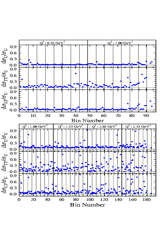
Figure 13: (Color online) Total kinematic-independent systematic uncertainties from eq.(8) on the structure functions $\sigma_{U}$, $\sigma_{TT}$, and $\sigma_{LT}$ normalized to $\sigma_{U}$ for the $K^{+}\Lambda$ data as a function of bin number for the 2.567 GeV (top) and 4 GeV (bottom) data sets. The wide vertical boundaries indicate the $Q^{2}$ bins, the narrow vertical boundaries indicate the $W$ bins within each $Q^{2}$ range, and the six points in each $W$ bin represent the angle bins from $\cos\theta_{K}^{*}$=-0.65 to 0.90.

		Systematic Uncertainty
Beam Energy	Term	$Q^{2}$=0.65 GeV2		$Q^{2}$=1.00 GeV2
2.567 GeV	$\delta\sigma_{U}/\sigma_{U}$	9.6%		8.4%
	$\delta\sigma_{TT}/\sigma_{U}$	11.7%		10.8%
	$\delta\sigma_{LT}/\sigma_{U}$	7.8%		6.3%
Beam Energy	Term	$Q^{2}$=1.00 GeV2		$Q^{2}$=1.55, 2.05, 2.55 GeV2
4 GeV	$\delta\sigma_{U}/\sigma_{U}$	$W$=1.65 GeV	13.9%	8.4%
		1.75 GeV	10.8%
		$\geq 1.85$ GeV	10%
	$\delta\sigma_{TT}/\sigma_{U}$	$W$=1.65 GeV	15.4%	10.8%
		1.75 GeV	12.7%
		$\geq 1.85$ GeV	12%
	$\delta\sigma_{LT}/\sigma_{U}$	$W$=1.65 GeV	12.7%	6.3%
		1.75 GeV	9.3%
		$\geq 1.85$ GeV	8%

Table 4: Total systematic uncertainties assigned to our structure function measurements for both the $K^{+}\Lambda$ and $K^{+}\Sigma^{0}$ final states as a function of kinematics. Uncertainties for $\sigma_{U}$, $\sigma_{TT}$, and $\sigma_{LT}$ are all quoted relative to $\sigma_{U}$.

The systematic uncertainty analysis on the separated structure functions $\sigma_{T}$ and $\sigma_{L}$ was carried out only for the Rosenbluth separation method. In order to be conservative, the same systematic uncertainty is assigned to $\sigma_{T}$ and $\sigma_{L}$ extracted from the simultaneous $\epsilon-\Phi$ fit. This was done as we could not fully disentangle the point-to-point and scale-type systematic uncertainties between the two beam energy data sets in the $\epsilon-\Phi$ fits. In this analysis, we simply use the two different techniques as a way to perform a consistency check on our extracted structure functions. Our analysis shows very good agreement between the two techniques giving us confidence in our assigned systematics.

We performed several consistency checks on our data. The most important were that cross sections at 2.567 GeV taken with two different magnetic field settings and our cross sections taken at 4.056 and 4.247 GeV agreed within the quoted systematics. This tested the accuracy of our knowledge of the acceptance because it varied strongly with field setting and beam energy. The other check was to fit the two beam energy data sets simultaneously in each of our bins to verify that the relative normalization factor between the two data sets was consistent with unity.

VIII Results

VIII.1 Three Structure Function Separation

VIII.1.1 Angular Dependence

In Figs. 14 and 15 we show the extracted structure functions $\sigma_{U}$, $\sigma_{TT}$, and $\sigma_{LT}$ versus $\cos\theta_{K}^{*}$ for $K^{+}\Lambda$ and $K^{+}\Sigma^{0}$ for different $W$ points at $Q^{2}$=0.65 GeV² from our 2.567 GeV data set. Although we focus on the $\cos\theta_{K}^{*}$ dependence of our low $Q^{2}$ data set at 2.567 GeV, the general conclusions that can be drawn from studying the angular dependence are similar for our other data sets. However, the full set of our data is available in Ref. database . In these plots, the data are sorted into $W$ bins 50-MeV wide, except for the first and last $W$ bins which are 100-MeV wide (see Table 2). All data points have been evolved to the given $Q^{2}$, $W$, and $\cos\theta_{K}^{*}$ bin centers. The curves shown are from the hadrodynamic models of Bennhold and Mart (BM) bm_calc (dot-dashed curves) and of Janssen et al. (JB) jb_calc (solid curves), and the Reggeon-exchange model of Guidal et al. (GLV) glv_calc (dashed curves).

Figure 14: Structure functions $\sigma_{U}$, $\sigma_{TT}$, and $\sigma_{LT}$ (in nb/sr) for $K^{+}\Lambda$ production vs. $\cos\theta_{K}^{*}$ at 2.567 GeV for $Q^{2}$=0.65 GeV² and $W$ from 1.650 to 2.050 GeV. The error bars represent the statistical uncertainties only. The relative systematic uncertainties to $\sigma_{U}$ are given in Table 4. The curves shown are from the model calculations of Bennhold and Mart (BM)  bm_calc (dot-dashed), Janssen et al. (JB) jb_calc (solid), and Guidal et al. (GLV) glv_calc (dashed). The models are described in the text.

Figure 15: Structure functions $\sigma_{U}$, $\sigma_{TT}$, and $\sigma_{LT}$ (in nb/sr) for $K^{+}\Sigma^{0}$ production vs. $\cos\theta_{K}^{*}$ at 2.567 GeV for $Q^{2}$=0.65 GeV² and $W$ from 1.725 to 2.050 GeV. The error bars represent the statistical uncertainties only. The relative systematic uncertainties to $\sigma_{U}$ are given in Table 4. The curves shown are from the model calculations of Bennhold and Mart (BM)  bm_calc (dot-dashed), Janssen et al. (JB) jb_calc (solid), and Guidal et al. (GLV) glv_calc (dashed). The models are described in the text.

A number of observations can be made independent of the model calculations. First, we observe that the $K^{+}\Lambda$ and $K^{+}\Sigma^{0}$ electroproduction dynamics are very different. The data in Figs. 14 and 15 reveal that $\sigma_{U}$ is more forward-peaked in $K^{+}\Lambda$ production than for $K^{+}\Sigma^{0}$ production across our full range in $W$. With regard to the interference structure functions, $\sigma_{TT}$ for $K^{+}\Lambda$ is roughly one-fourth of $\sigma_{U}$ and always negative and very similar in structure and magnitude to $\sigma_{LT}$, while $\sigma_{TT}$ for $K^{+}\Sigma^{0}$ is generally smaller in magnitude than for $K^{+}\Lambda$ with a peaking at more mid-range angles. The $K^{+}\Lambda$ reaction has a significant $\sigma_{LT}$ component in the forward direction compared to $\sigma_{U}$, while $\sigma_{LT}$ for the $K^{+}\Sigma^{0}$ reaction is everywhere consistent with zero.

The forward-peaking of $\sigma_{U}$ and $\sigma_{LT}$ for $K^{+}\Lambda$ compared to $K^{+}\Sigma^{0}$ can be qualitatively explained by the effect of the longitudinal coupling of the virtual photons. We note that the two channels are of nearly equal strength at $Q^{2}$=0 GeV² mcnabb ; bradford1 , while here at $Q^{2}$=0.65 GeV² the $K^{+}\Lambda$ channel is stronger than the $K^{+}\Sigma^{0}$ channel at forward angles by a factor of 2 to 3. For transverse (real) photons, the $t$-channel mechanism at low $t$ is dominated by vector $K^{*+}$ exchange, which relates directly to the relative magnitudes of the $g_{K^{*}YN}$ coupling constants to the $g_{KYN}$ constants. As $Q^{2}$ rises from zero, the photon can acquire a longitudinal polarization and the importance of pseudoscalar $K^{+}$ exchange increases. Given that $g_{K\Lambda N}^{2}\gg g_{K\Sigma^{0}N}^{2}$ adel_saghai ; deswart , this effect increases the cross section for $K^{+}\Lambda$ relative to $K^{+}\Sigma^{0}$. This argument was already noted in the earliest reports of hyperon electroproduction brown , and is strengthened by our observation of a sizeable $\sigma_{LT}$ for $K^{+}\Lambda$ and a $\sigma_{LT}$ consistent with zero for $K^{+}\Sigma^{0}$. It should also be the case that since $g_{K^{*}\Sigma N}\gg g_{K\Sigma N}$, $K^{*}$ exchange should dominate the $\Sigma^{0}$ channel. Because $K^{*}$ exchange must vanish at forward angles due to angular momentum conservation, the $\Sigma^{0}$ cross section should also decrease at forward angles guidal .

None of the three different models shown is particularly successful at describing all of the data. In general the models better agree with the $K^{+}\Lambda$ data than with the $K^{+}\Sigma^{0}$ data. The three models tend to reproduce the qualitative fall-off in $\cos\theta_{K}^{*}$ of $\sigma_{U}$ for the $K^{+}\Lambda$ data but do not include sufficient forward-angle strength for $W<1.8$ GeV. At higher $W$ the BM model generally reproduces $\sigma_{U}$, while the JB model consistently is too large at forward and backward kaon angles. The GLV model goes above our data as $\cos\theta_{K}^{*}\to 1$, but describes the structure of the $K^{+}\Lambda$ data surprisingly well considering that it has no built-in $s$-channel resonances. $\sigma_{U}$ for the $K^{+}\Sigma^{0}$ data is poorly described by all models, especially the JB model, which includes too much $u$-channel strength, while the BM and GLV models generally include too little strength or miss the broad peaking about $\cos\theta_{K}^{*}\sim 0$.

Within the GLV Regge model, the functions $\sigma_{TT}$ and $\sigma_{LT}$ arise from the interference of the $K$ and $K^{*}$ Regge trajectories. This modeling is sufficient to qualitatively reproduce the behavior of both the $K^{+}\Lambda$ and $K^{+}\Sigma^{0}$ data over our full kinematic phase space. The quality of the comparisons of the hadrodynamic models to the $\sigma_{TT}$ and $\sigma_{LT}$ data are much less favorable. For the JB model, $\sigma_{TT}$ for $K^{+}\Lambda$ has the correct sign, but its strength is too small and the angular dependence does not match the data. For $K^{+}\Sigma^{0}$, the JB model predicts $\sigma_{TT}\sim 0$ everywhere, in strong disagreement with the data. For the BM model, $\sigma_{TT}$ for $K^{+}\Lambda$ has a strength and angle dependence that qualitatively matches the data, but has the wrong sign. For $K^{+}\Sigma^{0}$, the BM model has the wrong sign for $\sigma_{TT}$ and doesn’t match the angular distribution of the data. From the JB model, $\sigma_{LT}$ for $K^{+}\Lambda$ is consistent with zero at low $W$, but increases in strength for higher $W$, where the model has the wrong sign compared to the data. For $K^{+}\Sigma^{0}$, the JB model has both the wrong sign and angular dependence. For the BM model, $\sigma_{LT}$ follows the trends of the $K^{+}\Lambda$ data but has overall too little strength, while it is reasonably consistent with the $K^{+}\Sigma^{0}$ data.

VIII.1.2 Energy Dependence

Even if $\Lambda$ production for forward-going $K^{+}$ mesons is dominated by $t$-channel exchange, there is still room for $s$-channel resonance contributions at more central angles and at all angles for the $\Sigma^{0}$. To more directly look for $s$-channel resonance evidence, the extracted structure functions are presented as a function of the center-of-mass energy $W$ for our six bins in $\cos\theta_{K}^{*}$. Figures 16 and 17 show the results for our 2.567 GeV data at $Q^{2}$=0.65 GeV² for the contiguous angle bins centered at $\cos\theta_{K}^{*}$ = -0.6, -0.25, 0.05, 0.35, 0.65, and 0.90.

Figure 16: Structure functions $\sigma_{U}$, $\sigma_{TT}$, and $\sigma_{LT}$ (in nb/sr) for $K^{+}\Lambda$ production vs. $W$ at 2.567 GeV for $Q^{2}$=0.65 GeV² for our 6 $\cos\theta_{K}^{*}$ bins. The error bars represent the statistical uncertainties only. The relative systematic uncertainties to $\sigma_{U}$ are given in Table 4. The curves shown are from the model calculations of Bennhold and Mart (BM) bm_calc (dot-dashed), Janssen et al. (JB) jb_calc (solid), and Guidal et al. (GLV) glv_calc (dashed). The models are described in the text. The data (and calculations) for $\sigma_{U}$ for the two back-angle points have been scaled by a factor of 3 for clarity.

Figure 17: Structure functions $\sigma_{U}$, $\sigma_{TT}$, and $\sigma_{LT}$ (in nb/sr) for $K^{+}\Sigma^{0}$ production vs. $W$ at 2.567 GeV for $Q^{2}$=0.65 GeV² for our 6 $\cos\theta_{K}^{*}$ bins. The error bars represent the statistical uncertainties only. The relative systematic uncertainties to $\sigma_{U}$ are given in Table 4. The curves shown are from the model calculations of Bennhold and Mart (BM) bm_calc (dot-dashed), Janssen et al. (JB) jb_calc (solid), and Guidal et al. (GLV) glv_calc (dashed). The models are described in the text.

Several characteristics of the data stand out. For $K^{+}\Lambda$ production, $\sigma_{U}$ shows a broad peak at about 1.7 GeV at forward angles, and two peaks separated by a dip at about 1.75 GeV for our two backward angle points. Across our phase space, $\sigma_{TT}$ and $\sigma_{LT}$ for $K^{+}\Lambda$ production are predominantly negative and about one-third the size of $\sigma_{U}$. Where the statistical uncertainties on our data are reasonable (away from the most forward-angle point), $\sigma_{TT}$ and $\sigma_{LT}$ seem to be similar in shape to $\sigma_{U}$, but opposite in sign. The $K^{+}\Sigma^{0}$ structure functions have a different set of features. Both $\sigma_{U}$ and $\sigma_{TT}$ exhibit a broad bump at about 1.85 GeV, while $\sigma_{LT}$ is consistent with zero everywhere. The $\Sigma^{0}$ shapes are similar for both forward and back-angle production, with a strong peaking at central angles.

We argue here that our spectra likely reflect the existence of a few underlying $s$-channel resonances along with $t$-channel processes, but acknowledge that the physical interpretation is not straightforward and will require detailed modeling. The $W$-dependence of the $K^{+}\Lambda$ data for $\sigma_{U}$ near threshold shows more structure than a model based upon only $t$-channel exchanges provides (GLV model - dashed curves) and is probably evidence of resonance activity. In this range of $W$, the $S_{11}(1650)$ is believed to be dominant in the $s$-channel bennhold . There are also a number of known $N^{*}$ resonances near 1.7 GeV that can contribute to the $K^{+}\Lambda$ and $K^{+}\Sigma^{0}$ final states, in particular, the $P_{11}(1710)$ and $P_{13}(1720)$. The effect of these resonances can be seen in the hadrodynamic model calculations (BM model - dot-dashed curves, JB model - solid curves), though clearly their strengths at the measured $Q^{2}$ are not correct.

The double-peaking of $\sigma_{U}$ for $K^{+}\Lambda$ production at backward $\theta_{K}^{*}$ angles as seen in Fig. 16, corroborates a similar structure seen in recent photoproduction results saphir1 ; saphir2 ; mcnabb ; bradford1 . Within existing hadrodynamic models, the structure just above the threshold region is typically accounted for by the known $S_{11}$(1650), $P_{11}$(1710), and $P_{13}$(1720) nucleon resonances. However there is no consensus as to the origin of the bump feature at $\sim$1.9 GeV that was first seen in the $K^{+}\Lambda$ photoproduction data from SAPHIR saphir1 . It is tempting to speculate that this is evidence for a previously “missing”, negative-parity $J=3/2$ resonance at 1.96 GeV predicted in the quark model of Capstick and Roberts capstick . This explanation was put forward in the work of Bennhold and Mart bennhold , in which they postulated the existence of a $D_{13}$ state at 1.9 GeV. However, other groups have shown that the same data can also be explained by accounting for $u$-channel hyperon exchanges saghai1 or with an additional $P$-wave resonance janssen2 . From our data, the $W$ spectra of the interference terms, $\sigma_{TT}$ and $\sigma_{LT}$, show no clear structures in the region about 1.9 GeV, whereas an $s$-channel resonance would likely be reflected in the structure of the interference terms, particularly $\sigma_{TT}$. Note that the BM and JB models include a $D_{13}$(1895) resonant state whose coupling strength was determined from fits to the SAPHIR $K^{+}\Lambda$ total cross section data saphir1 ; saphir2 . Clearly the differences between both models and our data indicate that either the resonance parameters are not accurate, that more resonant terms are required, or that the bump at 1.9 GeV in our $W$ spectra has a non-resonant origin. We conclude that the $W$ dependence of $K^{+}\Lambda$ production provides suggestive evidence for baryon resonance activity within the reaction mechanism, but that the data in comparison to present models does not allow any simple statement to be made.

In the $K^{+}\Sigma^{0}$ channel, $\sigma_{U}$ is peaked at about 1.85 GeV, which also matches the photoproduction result saphir2 ; mcnabb . In addition, $\sigma_{TT}$ shows a broad feature in this same region. These features are consistent with a predominantly $s$-channel production mechanism. In this region, beyond the specific $N^{*}$ resonances believed to contribute to $K^{+}\Lambda$ production (and hence are strong candidates to contribute to $K^{+}\Sigma^{0}$ production), there are a number of known $\Delta^{*}$ resonances near 1.9 GeV pdg that can contribute to the $K^{+}\Sigma^{0}$ final state, particularly the $\Delta^{*}$(1900) and $\Delta^{*}$(1910). These $\Delta^{*}$ states are forbidden to couple to the $K^{+}\Lambda$ state due to isospin conservation. Current hadrodynamic models seem to indicate that both $N^{*}$ and $\Delta^{*}$ states (see Table 1) are necessary to describe the existing photo- and electroproduction data.

The comparison of the hadrodynamic model calculations to the data clearly indicates that significant new constraints on the model parameters will be brought about when these new data are included in the fits. The models do not reproduce $\sigma_{U}$, $\sigma_{TT}$, or $\sigma_{LT}$ at any level, especially for the $K^{+}\Sigma^{0}$ data. The Regge model tends to underpredict the strength of $\sigma_{U}$ across the full angular range, which is suggestive of $s$-channel contributions to this reaction. Again the trends of $\sigma_{TT}$ and $\sigma_{LT}$ are reasonably well reproduced with the inclusion of only the $K$ and $K^{*}$ Regge trajectories.

VIII.1.3 $Q^{2}$ Dependence

The data shown in Figs. 16 and 17 were obtained from our 2.567 GeV data set at $Q^{2}$=0.65 GeV². Our data set at 4 GeV provides a much larger $Q^{2}$ reach and it is instructive to study the $W$ spectra for increasing values of $Q^{2}$. These data are shown in Figs. 18 and 19 for one of our backward-angle points ($\cos\theta_{K}^{*}$=-0.25) and a more forward-angle point ($\cos\theta_{K}^{*}$=0.35). The interference structure functions (not shown) do not have a strong $Q^{2}$ dependence, while $\sigma_{U}$ shows a smooth fall-off. Note that at $Q^{2}$=1.0 GeV², our back-angle data do not show the double-peaked structure that was evident at $Q^{2}$=0.65 GeV² (see Fig. 16) and also in our $Q^{2}$=1.0 GeV² data at 2.567 GeV (not shown). This could be due to our increased $W$ bin width at 4 GeV (100 MeV compared to 50 MeV at 2.567 GeV), or could imply a strong $\epsilon$ dependence to the resonance strength.

Figure 18: $W$ distributions of $\sigma_{U}$ for the $K^{+}\Lambda$ final state from our 4 GeV data set (evolved to 4.056 GeV) for each of our four points in $Q^{2}$ for $\cos\theta_{K}^{*}$=-0.25 (left) and 0.35 (right). The relative systematic uncertainties to $\sigma_{U}$ are given in Table 4. The curves shown are from the model calculations of Bennhold and Mart (BM) bm_calc (dot-dashed), Janssen et al. (JB) jb_calc (solid), and Guidal et al. (GLV) (dashed).

Figure 19: $W$ distributions of $\sigma_{U}$ for the $K^{+}\Sigma^{0}$ final state from our 4 GeV data set (evolved to 4.056 GeV) for each of our four points in $Q^{2}$ for $\cos\theta_{K}^{*}$=-0.25 (left) and 0.35 (right). The relative systematic uncertainties to $\sigma_{U}$ are given in Table 4. The curves shown are from the model calculations of Bennhold and Mart (BM) bm_calc (dot-dashed), Janssen et al. (JB) jb_calc (solid), and Guidal et al. (GLV) (dashed).

None of the models reproduces the $K^{+}\Lambda$ data in detail. Both hadrodynamic models are very poor matches to these data, while the GLV Regge model tends to underpredict the strength in our more forward angle point, although it is in fair agreement with the data in our more backward angle point. For the $K^{+}\Sigma^{0}$ data none of the models shown reproduce even the qualitative aspects of the data.

The $Q^{2}$ dependence of $\sigma_{U}$ for $K^{+}\Lambda$ and $K^{+}\Sigma^{0}$ can be studied within our 4 GeV data set as shown in Fig. 20. The data shown are from our points at $\cos\theta_{K}^{*}$=-0.25 and 0.90 for three different $W$ values across the nucleon resonance region. Also included on these plots are our two data points from the 2.567 GeV data set at $Q^{2}$=0.65 GeV² and 1.00 GeV², along with the CLAS $\sigma_{T}$ data from photoproduction at $Q^{2}$=0 from Bradford et al. bradford1 . No clear features are apparent here, with the data showing a smooth fall-off with respect to the photon point with increasing $Q^{2}$ for both final states except for the forward-angle $K^{+}\Lambda$ data at $W$=1.75 GeV. In order to compare more directly with the existing measurements from the 1970’s (taken for $\theta_{K}^{*}<15^{\circ}$, $0.5<Q^{2}<4.0$ GeV², and evolved to $W$=2.15 GeV) compiled by Bebek et al. in Ref. bebek2 , we have fit our 4 GeV $\sigma_{U}$ data with the dipole form $C/(Q^{2}+M^{2})^{2}$ (where $C$ is an arbitrary constant and the CLAS photoproduction data are not included in the fits) and compared the mass terms to those extracted from the fits in Ref. bebek2 . Fits to the older data suggested that the $K^{+}\Sigma^{0}$ data with $M^{2}=(0.785\pm 0.095)$ GeV² fell off more rapidly with increasing $Q^{2}$ than the $K^{+}\Lambda$ data with $M^{2}=(2.67\pm 0.28)$ GeV². The results from our fits are contained in Table 5 and shown in Fig. 20. Our extracted mass terms, even for backward angles where $s$-channel and $u$-channel contributions are expected to be more important relative to $t$-channel kaon exchange, are consistent with the fits of Ref. bebek2 extracted from forward kaon angle data. These results highlight the fact that the production mechanisms for $K^{+}\Lambda$ and $K^{+}\Sigma^{0}$ are quite different.

		$K^{+}\Lambda$	$K^{+}\Sigma^{0}$
$\cos\theta_{K}^{*}$	$W$ (GeV)	$M^{2}$ (GeV2)	$M^{2}$ (GeV2)
-0.25	1.75	$1.81\pm 0.48$	$1.58\pm 1.18$
-0.25	1.85	$1.34\pm 0.37$	$0.41\pm 0.22$
-0.25	1.95	$1.41\pm 0.54$	$0.64\pm 0.28$
0.90	1.75	$1.75\pm 0.21$	–
0.90	1.85	$2.75\pm 0.38$	$1.51\pm 1.46$
0.90	1.95	$2.09\pm 0.35$	$1.25\pm 1.45$

Table 5: Mass terms from the fit to our $\sigma_{U}$ structure functions vs. $Q^{2}$ (not including the photoproduction points). A dipole form of $C(Q^{2}+M^{2})^{-2}$ is employed.

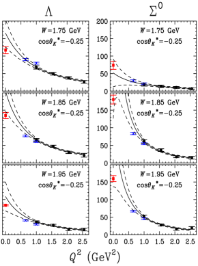
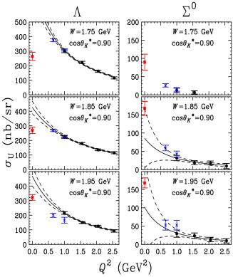
Figure 20: (Color online) $Q^{2}$ distributions of $\sigma_{U}$ for the $K^{+}\Lambda$ and $K^{+}\Sigma^{0}$ final states from our 4 GeV data set (dark filled circles – evolved to 4.056 GeV) at $\cos\theta_{K}^{*}$=-0.25 (left) and 0.90 (right) for $W$=1.750 GeV (top), 1.850 GeV (middle), and 1.950 GeV (bottom). The solid curves are from a dipole mass fit to the 4 GeV data of the form $C(Q^{2}+M^{2})^{-2}$. The $Q^{2}$=0 points (solid squares) come from Bradford et al. bradford1 and the two data points from our 2.567 GeV data (light crosses) are not included in the fits. The dashed lines represent the error bands from the fits.

It is interesting to see that the $Q^{2}$ fits for the $K^{+}\Lambda$ data significantly overshoot the photon point for our forward angle data. In the absence of other knowledge, one might speculate that this is entirely due to a significant contribution to the cross section from $\sigma_{L}$. However, when the points from the 2.567 GeV data set are included on the plot, we see that they fall near the curve fit to our 4 GeV data for all points for $K^{+}\Lambda$ and $K^{+}\Sigma^{0}$ except our highest $W$ point for $K^{+}\Lambda$. This suggests a small contribution from $\sigma_{L}$. Indeed, the $\sigma_{L}$/$\sigma_{T}$ separations shown in the next section verify this. Janssen et al. janssen1 have calculated a fall off in $\sigma_{T}$ near $Q^{2}$=0, as indicated by our data. This was accomplished by including a $Q^{2}$ dependence to the kaon and proton form factors.

VIII.2 $\sigma_{T}$ and $\sigma_{L}$ Separation

Our analysis results for $\sigma_{T}$ and $\sigma_{L}$ are presented in Fig. 21 for the $K^{+}\Lambda$ final state and in Fig. 22 for the $K^{+}\Sigma^{0}$ final state. The data are shown here in terms of the ratio $R=\sigma_{L}/\sigma_{T}$ as a function of $\cos\theta_{K}^{*}$ for our different $W$ values. For the $K^{+}\Lambda$ final state our analysis includes $W$ points from 1.65 to 1.95 GeV, and for the $K^{+}\Sigma^{0}$ final state our analysis includes $W$ points from 1.75 to 1.95 GeV. Note that the statistical quality of our data did not allow us to separate $\sigma_{L}$ and $\sigma_{T}$ at $W$=2.05 GeV. The figures show the ratio extraction using both the Rosenbluth and the simultaneous $\epsilon-\Phi$ fit techniques, and the error bars show both statistical and total statistical and systematic uncertainties. The discussion of systematic uncertainties on these quantities is included in Section VII.

The agreement between the Rosenbluth and simultaneous $\epsilon-\Phi$ fits is generally very good across our full $W$ and $\cos\theta_{K}^{*}$ phase space at $Q^{2}$ = 1.0 GeV². The ratio of $\sigma_{L}/\sigma_{T}$ for both the $K^{+}\Lambda$ and $K^{+}\Sigma^{0}$ final states shows $\sigma_{L}$ to be consistent with zero over our full kinematic range except in our highest $W$ point for the $K^{+}\Lambda$ reaction, where the value of $R$ varies between 0.5 and 1 depending on kaon angle. While several of the extracted values for $R$ are negative and might be considered ”unphysical”, the majority of these points are consistent with zero within the combined statistical and systematic uncertainties.

Our data at $W$=1.85 GeV and $\cos\theta_{K}^{*}$=0.90 are consistent with the parallel kinematics measurement of Mohring et al. mohring from Hall C which found $R=0.45^{+0.19}_{-0.16}$ for $K^{+}\Lambda$ and $R=0.29^{+0.54}_{-0.33}$ for $K^{+}\Sigma^{0}$ at $W$=1.84 GeV, as well as the recent Hall B results of Raue and Carman raue04 for $K^{+}\Lambda$ which found $R$=0.005$\pm$0.228, 0.239$\pm$0.343, and 0.088$\pm$0.480 for $\theta_{K}^{*}$=0^∘ and $W$=1.72, 1.84, and 1.98 GeV, respectively. Note that the quoted uncertainties on $R$ from Mohring et al. mohring and Raue and Carman raue04 given here represent the total statistical and systematic uncertainties.

Figure 21: Results for the ratio $R=\sigma_{L}/\sigma_{T}$ for the $K^{+}\Lambda$ reaction for the Rosenbluth technique (diamonds) and the simultaneous $\epsilon-\Phi$ fit (filled circles). The Rosenbluth results have been offset in angle for clarity. The data are plotted versus $\cos\theta_{K}^{*}$ for our four $W$ points at $Q^{2}$=1.0 GeV². The inner error bars are statistical only and the outer error bars are combined statistical and systematic. The curves shown are from the model calculations of Bennhold and Mart (BM) bm_calc (dot-dashed), Janssen et al. (JB) jb_calc (solid), and Guidal et al. (GLV) (dashed). The parallel kinematics data points come from Mohring et al. mohring (open square) and Raue-Carman raue04 (open triangles).

Figure 22: Results for the ratio $R=\sigma_{L}/\sigma_{T}$ for the $K^{+}\Sigma^{0}$ reaction for the Rosenbluth technique (diamonds) and the simultaneous $\epsilon-\Phi$ fit (filled circles). The Rosenbluth results have been offset in angle for clarity. The data are plotted versus $\cos\theta_{K}^{*}$ for our three $W$ points at $Q^{2}$=1.0 GeV². The inner error bars are statistical only and the outer error bars are combined statistical and systematic. The curves shown are from the model calculations of Bennhold and Mart (BM) bm_calc (dot-dashed), Janssen et al. (JB) jb_calc (solid), and Guidal et al. (GLV) (dashed). The parallel kinematics data point comes from Mohring et al. mohring (open square).

The predictions of the hadrodynamic models for the ratio $R$ are very sensitive to the dynamics included in the calculation. All models shown for the $K^{+}\Lambda$ final state predict $R$ to be less than unity. Given the size of the error bars on the data, all of the models can be said to be roughly consistent with the data. However it is clear that the JB model jb_calc predicts too much longitudinal strength at low $W$. Also for the highest $W$ point, where $R$ begins to increase, the BM model bm_calc predicts too little longitudinal strength. The GLV model glv_calc is in very good agreement with the data over the full kinematic range shown.

For the $K^{+}\Sigma^{0}$ final state, the JB model jb_calc disagrees with the measured ratio $R$, which will be shown to result from too little transverse strength. The BM model bm_calc also suffers from too little transverse strength for our two lowest $W$ points, but is consistent with the data at $W$=1.95 GeV. Again, the GLV model glv_calc agrees well with the data over the full kinematic range shown.

Clearly these data, even with their sizeable statistical and systematic uncertainties, can provide for important constraints on the underlying dynamics and production models for both the $K^{+}\Lambda$ and $K^{+}\Sigma^{0}$ final states.

The structure functions $\sigma_{T}$ and $\sigma_{L}$ are plotted separately in Figs. 23 and 24 for $K^{+}\Lambda$ as a function of $\cos\theta_{K}^{*}$. Here $\sigma_{T}$ has a similar trend in angle for all $W$ points, peaking at forward kaon angles and falling off smoothly as the angle increases. For $\sigma_{L}$, the strength is consistent with zero for our points in $W$ from 1.65 to 1.85 GeV. At $W$=1.95 GeV, $\sigma_{L}$ is comparable with $\sigma_{T}$ in its angular dependence and its strength. The data for $\sigma_{T}$ and $\sigma_{L}$ are consistent with the existing parallel kinematics measurement at $W$=1.85 GeV of Mohring et al. mohring from Hall C at JLab.

The comparison of the models to $\sigma_{T}$ for the $K^{+}\Lambda$ final state shows that they underpredict the data and the strength of the forward-angle rise for our two lowest $W$ points. For our two highest $W$ points, the calculations (with the exception of the JB model jb_calc at $W$=1.95 GeV) are in good agreement with the data. For $\sigma_{L}$, the calculations from the BM model bm_calc and the GLV model glv_calc are in reasonable agreement with the data given the error bars. However, the JB model jb_calc predicts too much longitudinal strength for the full kinematic range shown.

Figure 23: Structure function $\sigma_{T}$ vs. $\cos\theta_{K}^{*}$ for the $K^{+}\Lambda$ final state for our different $W$ points at $Q^{2}$=1.0 GeV² from the $\epsilon-\Phi$ fit. The inner error bars are statistical only and the outer error bars are combined statistical and systematic. The curves shown are from the model calculations of Bennhold and Mart (BM) bm_calc (dot-dashed), Janssen et al. (JB) jb_calc (solid), and Guidal et al. (GLV) (dashed). The parallel kinematics data point comes from Mohring et al. mohring (open square).

Figure 24: Structure function $\sigma_{L}$ vs. $\cos\theta_{K}^{*}$ for the $K^{+}\Lambda$ final state for our different $W$ points at $Q^{2}$=1.0 GeV² from the $\epsilon-\Phi$ fit. The inner error bars are statistical only and the outer error bars are combined statistical and systematic. The curves shown are from the model calculations of Bennhold and Mart (BM) bm_calc (dot-dashed), Janssen et al. (JB) jb_calc (solid), and Guidal et al. (GLV) (dashed). The parallel kinematics data point comes from Mohring et al. mohring (open square).

The structure functions $\sigma_{T}$ and $\sigma_{L}$ are plotted separately in Figs. 25 and 26 for $K^{+}\Sigma^{0}$ as a function of $\cos\theta_{K}^{*}$. $\sigma_{T}$ is seen to have a broad peaking at more central angles for $K^{+}\Sigma^{0}$ compared to the $K^{+}\Lambda$ final state and $\sigma_{L}$ is consistent with zero everywhere. The data for $\sigma_{T}$ and $\sigma_{L}$ are consistent with the existing parallel kinematics measurement at $W$=1.85 GeV of Mohring et al. mohring from Hall C at JLab.

The models compare poorly with the data for $\sigma_{T}$ for $K^{+}\Sigma^{0}$ underpredicting the strength of the data and missing the trends in the angular dependence. For $\sigma_{L}$, all models predict a small strength in agreement with the data. Given the size of the statistical and systematic error bars on the data, not much more can be said with respect to the model predictions.

Figure 25: Structure function $\sigma_{T}$ vs. $\cos\theta_{K}^{*}$ for the $K^{+}\Sigma^{0}$ final state for our different $W$ points at $Q^{2}$=1.0 GeV² from the $\epsilon-\Phi$ fit. The inner error bars are statistical only and the outer error bars are combined statistical and systematic. The curves shown are from the model calculations of Bennhold and Mart (BM) bm_calc (dot-dashed), Janssen et al. (JB) jb_calc (solid), and Guidal et al. (GLV) (dashed). The parallel kinematics data point comes from Mohring et al. mohring (open square).

Figure 26: Structure function $\sigma_{L}$ vs. $\cos\theta_{K}^{*}$ for the $K^{+}\Sigma^{0}$ final state for our different $W$ points at $Q^{2}$=1.0 GeV² from the $\epsilon-\Phi$ fit. The inner error bars are statistical only and the outer error bars are combined statistical and systematic. The curves shown are from the model calculations of Bennhold and Mart (BM) bm_calc (dot-dashed), Janssen et al. (JB) jb_calc (solid), and Guidal et al. (GLV) (dashed). The parallel kinematics data point comes from Mohring et al. mohring (open square).

IX Conclusions

We have measured $K^{+}\Lambda$ and $K^{+}\Sigma^{0}$ electroproduction over a wide range of kinematics in the nucleon resonance region, including first-reported measurements over the full range of kaon angle. We have presented data for the separated structure functions $\sigma_{T}$, $\sigma_{L}$, and the interference structure functions $\sigma_{LT}$ and $\sigma_{TT}$. We conclude that $K^{+}\Lambda$ and $K^{+}\Sigma^{0}$ electroproduction dynamics are markedly different. We find that $\sigma_{U}$ ($=\sigma_{T}+\epsilon\sigma_{L}$) and $\sigma_{TT}$ are forward-peaked (in kaon angle) for the $K^{+}\Lambda$ final state and peaked at more central angles for $K^{+}\Sigma^{0}$, with $\sigma_{TT}$ a significant fraction of $\sigma_{U}$ for both hyperon final states. For the $K^{+}\Lambda$ channel, $\sigma_{LT}$ is a significant fraction of $\sigma_{U}$ and negative, while it is consistent with zero for the $K^{+}\Sigma^{0}$ channel.

The $W$ dependence of $\sigma_{U}$ for $K^{+}\Sigma^{0}$ shows a broad enhancement at $W\sim$ 1.85 GeV for $\sigma_{U}$ and $\sigma_{TT}$, presumably due to the various $\Delta^{*}$ resonances in this mass region. The $W$ dependence for $K^{+}\Lambda$ production is more complicated, evolving from a single-peaked structure at forward angles to a double-peaked structure at backward angles at low $Q^{2}$, with the double-peaking not obvious above $Q^{2}$=1.0 GeV². The longitudinal structure function $\sigma_{L}$ is consistent with zero for $K^{+}\Lambda$ across our full kinematic space except for our highest $W$ point at 1.95 GeV, and is consistent with zero everywhere for our $K^{+}\Sigma^{0}$ data. The transverse structure function $\sigma_{T}$ is forward-peaked for $K^{+}\Lambda$ and peaked at more central angles for $K^{+}\Sigma^{0}$.

The $Q^{2}$ dependence of the structure functions is unremarkable; the relatively slow fall-off, presumably reflecting the form factors of the various exchanged kaons in the case of $t$-channel processes, and the analogous baryonic form-factors in $s$ and $u$-channel processes. Of interest is our observation that an extrapolation of $\sigma_{U}$ to $Q^{2}=0$ overshoots the photoproduction value for $\sigma_{T}$. The obvious conjecture that this reveals the presence of a large value of $\sigma_{L}$ is not consistent with our direct measurements of $\sigma_{L}$, at least for lower values of $W$.

Detailed calculations are needed in order to investigate whether our data indicate the presence of any new $N^{*}$ resonances in $K^{+}\Lambda$ production. At the same time, the calculations must be able to fit the strong peak seen for $K^{+}\Sigma^{0}$ production and the shape of $\sigma_{TT}$ and $\sigma_{LT}$ in both channels. The question of the presence of any new resonances must wait for further work with the existing hadrodynamic models and partial wave analyses applied to the full range of our data. Fortunately, the new information we present here, especially the interference terms, will impose stringent constraints on the amplitudes used to model electroproduction of $K^{+}\Lambda$ and $K^{+}\Sigma^{0}$ final states, making these models more reliable for future interpretation and prediction.

We would like to acknowledge the outstanding efforts of the staff of the Accelerator and the Physics Divisions at JLab that made this experiment possible. This work was supported in part by the U.S. Department of Energy, the National Science Foundation, the Istituto Nazionale di Fisica Nucleare, the French Centre National de la Recherche Scientifique, the French Commissariat à l’Energie Atomique, and the Korean Science and Engineering Foundation. The Southeastern Universities Research Association (SURA) operated Jefferson Lab under United States DOE contract DE-AC05-84ER40150 during this work.

References

- (1) R. Koniuk and N. Isgur, Phys. Rev. D 21, 1868 (1980).
- (2) S. Capstick and W. Roberts, Phys. Rev. D 58, 1 (1998).
- (3) E. Klempt, nucl-ex/0203002, and references therein.
- (4) T.-S.H. Lee and T. Sato, Proceedings of the NSTAR 2000 Conference, eds. V.D. Burkert, L. Elouadrhiri, J.J. Kelly, and R. Minehart, (World Scientific, Singapore, 2001), p. 215.
- (5) CLAS data base, URL: http://clasweb.jlab.org/physicsdb.
- (6) Some authors use a pre-factor for the () term of () instead, where parameterizes the longitudinal polarization of the virtual photon. Some also take a () term out of the definition of ().
- (7) G. Knöchlein, D. Drechsel, and L. Tiator, Z. Phys. A 352, 327 (1995).
- (8) C.N. Brown et al., Phys. Rev. Lett. 28, 1086 (1972).
- (9) C.J. Bebek et al., Phys. Rev. Lett. 32, 21 (1974).
- (10) T. Azemoon et al., Nucl. Phys. B 95, 77 (1975).
- (11) C.J. Bebek et al., Phys. Rev. D 15, 594 (1977); C.J. Bebek et al., Phys. Rev. D 15, 3082 (1977).
- (12) F.E. Close, Nucl. Phys. B 73, 410 (1974); O. Nachtmann, Nucl. Phys. B74, 422 (1974); J. Cleymans and F.E. Close, Nucl. Phys. B 85, 429 (1975).
- (13) P. Brauel et al., Z. Phys. C 3, 101 (1979).
- (14) R.M. Mohring et al., Phys. Rev. C 67, 055205 (2003); reanalysis of G. Niculescu et al., Phys. Rev. Lett. 81, 1805 (1998).
- (15) Marius Coman, Ph.D. thesis, Florida International University (unpublished), (2005).
- (16) D.S. Carman et al. (CLAS Collaboration), Phys. Rev. Lett. 90, 131804 (2003).
- (17) Brian A. Raue and Daniel S. Carman, Phys. Rev. C 71, 065209 (2005).
- (18) M.Q. Tran et al., Phys. Lett. B 445, 20 (1998).
- (19) K.H. Glander et al., Eur. Phys. J. A 19, 251 (2004).
- (20) J. W. C. McNabb et al. (CLAS Collaboration), Phys. Rev. C 69, 042201(R) (2004).
- (21) R.K. Bradford et al. (CLAS Collaboration), Phys. Rev. C 73, 035202 (2006).
- (22) R.K. Bradford, Ph.D. thesis, Carnegie Mellon University (2005) (unpublished). Available at www.jlab.org/Hall-B/general/clas_thesis.html.
- (23) M. Sumihama et al. (LEPS Collaboration), Phys. Rev. C 73, 035214 (2006); R.T.G. Zegers et al. (LEPS Collaboration), Phys. Rev. Lett. 91, 092001 (2003).
- (24) H. Kohri et al. (LEPS Collaboration), Preprint hep-ex/0602015 (2006).
- (25) S. Janssen et al., Phys. Rev. C 67, 052201 (2003).
- (26) T. Mart and C. Bennhold, Phys. Rev. C 61, 012201 (2000).
- (27) H. Haberzettl et al., Phys. Rev. C 58, R40 (1998).
- (28) S. Janssen et al., Eur. Phys. J. A 11, 105 (2001); S. Janssen et al., Phys. Rev. C 65, 015201 (2001).
- (29) S. Janssen, Ph.D. Thesis, University of Gent, (2002).
- (30) F. Gross and D. Riska, Phys. Rev. C 36, 1928 (1987).
- (31) B. Saghai, AIP Conf. Proc. 594, 57 (2001).
- (32) D.G. Ireland, S. Janssen, and J. Ryckebusch, Nucl. Phys. A 740, 147 (2004).
- (33) A.V. Sarantsev et al., Eur. Phys. J. A 25, 427 (2005).
- (34) M. Guidal, J.M. Laget, and M. Vanderhaeghen, Phys. Rev. C 61, 025204 (2000).
- (35) M. Guidal, J.M. Laget, and M. Vanderhaeghen, Nucl. Phys. A 627, 645 (1997).
- (36) B.A. Mecking et al., Nucl. Inst. and Meth. A 503, 513 (2003).
- (37) M.D. Mestayer et al., Nucl. Inst. and Meth. A 449, 81 (2000).
- (38) G. Adams et al., Nucl. Inst. and Meth. A 465, 414 (2001).
- (39) E.S. Smith et al., Nucl. Inst. and Meth. A 432, 265 (1999).
- (40) M. Amarian et al., Nucl. Inst. and Meth. A 460, 460 (2001).
- (41) R. Brun et al., CERN-DD-78-2-REV, (1978).
- (42) L.W. Mo and Y. Tsai, Rev. Mod. Phys. 41, 205 (1969); Y.S. Tsai, Preprint SLAC, PUB-848, 1971.
- (43) R. Ent et al., Phys. Rev. C 64, 054610 (2001).
- (44) EXCLURAD code is based upon A. Afanasev et al., Phys. Rev. D 66, 074004 (2002).
- (45) Code from T. Mart, private communication, (2000), based upon the model of Ref. bennhold .
- (46) Code from model of S. Janssen, private communication, (2002), corresponding to Ref. janssen1 ; janssen2 . We show Model “B”.
- (47) Curves from model code of M. Guidal, private communication,(2000), corresponding to Ref. guidal .
- (48) R.A. Adelseck and B. Saghai, Phys. Rev. C 42, 108 (1990).
- (49) J.J. deSwart, Rev. Mod. Phys. 35, 916 (1963).
- (50) B. Saghai, nucl-th/0105001, (2001).
- (51) E.J. Weinberg and D.L. Nordstrom, Phys. Rev. D 66, 01001 (2002).