$\chi_{cJ}$ Decays to $h^{+}h^{-}h^{0}$

Abstract

Using a sample of $3\times 10^{6}$ $\psi(2S)$ decays recorded by the CLEO detector, we study three-body decays of the $\chi_{c0}$, $\chi_{c1}$, and $\chi_{c2}$ produced in radiative decays of the $\psi(2S)$. We consider the final states $\pi^{+}\pi^{-}\eta$, $K^{+}K^{-}\eta$, $p{\bar{p}}\eta$, $\pi^{+}\pi^{-}\eta^{\prime}$, $K^{+}K^{-}\pi^{0}$, $p{\bar{p}}\pi^{0}$, $\pi^{+}K^{-}K^{0}_{\rm S}$, and $K^{+}{\bar{p}}\Lambda$, measuring branching fractions or placing upper limits. For $\chi_{c1}\to\pi^{+}\pi^{-}\eta$, $K^{+}K^{-}\pi^{0}$, and $\pi^{+}K^{-}K^{0}_{\rm S}$ our observed samples are large enough to indicate the largest contributions to the substructure.

I Introduction

Decays of the $\chi_{c0}$, $\chi_{c1}$, and $\chi_{c2}$ states are not as well studied experimentally and theoretically as those of other charmonium states. These states have charge-conjugation eigenvalue $C=+1$, in contrast to the better-studied $C=-1$ states $J/\psi$ and $\psi(2S)$. Their decay products thus will differ from those of $J/\psi$ and $\psi(2S)$, and may provide complementary information on states containing light quarks and gluons. It is possible that the color-octet mechanism, $c\bar{c}g\to 2(q\bar{q})$, could have large effects on the observed decay pattern of the $\chi_{cJ}$ states quarkoniumreview . Assuming that $\chi_{cJ}$ are the ${}^{3}P_{J}$ $c\bar{c}$ bound states one would expect that $\chi_{c0}$ and $\chi_{c2}$ with $J^{PC}$ quantum numbers $0^{++}$ and $2^{++}$ decay to light quarks via two gluons Zhao . Measurement of any possible $\chi_{cJ}$ hadronic decays provides valuable information on possible glueball dynamics. Thus knowledge of any hadronic decay channels for these states is valuable.

CLEO has gathered a large sample of $e^{+}e^{-}\to\psi(2S)$ events, which leads to copious production of the $\chi_{cJ}$ states in radiative decays of the $\psi(2S)$. The $\psi(2S)$ branching fractions have been recently measured chicbf with high precision:

$${\mathcal{B}}(\psi(2S)\to\gamma\chi_{c0})=(9.22\pm 0.11\pm 0.46)\%;$$ (1)

$${\mathcal{B}}(\psi(2S)\to\gamma\chi_{c1})=(9.07\pm 0.11\pm 0.54)\%;$$ (2)

$${\mathcal{B}}(\psi(2S)\to\gamma\chi_{c2})=(9.33\pm 0.14\pm 0.61)\%.$$ (3)

We describe a study of selected three-body hadronic decay modes of the $\chi_{cJ}$ to two charged and one neutral hadron. This is not an exhaustive study of $\chi_{cJ}$ hadronic decays; we do not even comprehensively cover all possible $h^{+}h^{-}h^{0}$ decays, but simply take a first look at the rich structure of $\chi_{cJ}$ decays in our initial $\psi(2S)$ data sets. A subset of these modes has been investigated by BES BES . With the CLEO III detector configuration CLEOIII , we have recorded an integrated luminosity of 2.57 pb^-1 and the number of $\psi(2S)$ events is $1.56\times 10^{6}$. With the CLEO-c detector configuration CLEOc we have recorded 2.89 pb^-1, and the number of events is $1.52\times 10^{6}$. The apparent mis-match of luminosities and event totals is due to different beam energy spreads for the two data sets.

II Measurement of the branching fractions

Our basic technique is an exclusive whole-event analysis searching for $\psi(2S)\to\gamma\chi_{cJ}$ followed by a three body decay of the $\chi_{cJ}$ to $\pi^{+}\pi^{-}\eta$, $K^{+}K^{-}\eta$, $p{\bar{p}}\eta$, $\pi^{+}\pi^{-}\eta^{\prime}$, $K^{+}K^{-}\pi^{0}$, $p{\bar{p}}\pi^{0}$, $\pi^{+}K^{-}K^{0}_{\rm S}$, or $K^{+}{\bar{p}}\Lambda$. A photon candidate is combined with three hadrons and their 4-momentum sum constrained to the known total beam energy and the initial momentum caused by the two beams crossing at a small angle taking into account the measured errors on the reconstructed charged tracks, neutral hadron, and transition photon. We cut on the $\chi^{2}$ of this fit, which has four degrees of freedom, as it strongly discriminates between background and signal. For most modes we select events with an event 4-momentum fit $\chi^{2}$ less than 25, but background from $\psi(2S)\to J/\psi\pi^{0}\pi^{0}$ followed by charged two-body decays of the $J/\psi$, with one of the $\pi^{0}$ decay photons lost, fakes $\psi(2S)\to\gamma\chi_{cJ}\to\gamma p{\bar{p}}\pi^{0}$. For this mode the cut on $\chi^{2}$ is tightened to 12. The efficiency of this cut is $\approx$ 95% for all modes except $p{\bar{p}}\pi^{0}$, where it is $\approx$ 80%.

Efficiencies and backgrounds are studied in a GEANT-based simulation cleog of the detector response to $e^{+}e^{-}\to\psi(2S)$ events. Our simulated sample is roughly ten times our data sample. The radiated photon is generated according to an angular distribution of $1+\lambda\cos^{2}\theta$, where $\theta$ is the radiated photon angle relative to the positron beam axis. An E1 transition, as expected for $\psi(2S)\to\gamma\chi_{cJ}$, implies $\lambda=1,-1/3,+1/13$ for $J=0,1,2$ particles. The efficiencies we quote use this simulation, and differ from efficiencies using $\lambda=0$ by up to a few percent.

Photon candidates are selected by their energy depositions in the CsI crystal calorimeter. They have a transverse shape consistent with that expected for an electromagnetic shower without a charged track pointing toward it. They are required to have an energy of at least 30 MeV. Photon candidates that are used to make neutral particles further must have an energy of more than 50 MeV if they are not in the barrel, $|\cos\theta_{\gamma}|>0.82$, of our calorimeter. The $\pi^{0}\to\gamma\gamma$ and $\eta\to\gamma\gamma$ candidates are formed from two-photon candidates that are kinematically fit to the known resonance masses using the event vertex position, determined using charged tracks constrained to the beam spot. We select events with a $\chi^{2}$ from the kinematic mass fit with one degree of freedom of less than 10. Transition photon candidates are vetoed if they form a $\pi^{0}$ or $\eta$ candidate when paired with a second photon candidate.

We also reconstruct the $\eta\to\pi^{+}\pi^{-}\pi^{0}$ mode combining two charged pions with a $\pi^{0}\to\gamma\gamma$ candidate, increasing the number of $\eta$ candidates by about 25%. The same sort of kinematic mass fit as used for $\pi^{0}$’s and $\eta\to\gamma\gamma$ is applied to this mode, and again we select those giving a $\chi^{2}$ of less than 10. Similarly we combine the mass-constrained $\eta$ candidates together with two charged pions to make $\eta^{\prime}$ candidates, mass-constrain them, and select those with $\chi^{2}<10$. In addition, we include the decay mode $\eta^{\prime}\to\gamma\rho$. Here the background is potentially high because of the large number of noise photons, so we require $E_{\rm photon}>200$ MeV. In addition, we require the $\pi^{+}\pi^{-}$ mass to be within 100 MeV/c² of the mean $\rho$ mass.

Charged tracks satisfy standard requirements HadronicBF that they be of good fit quality. Those coming from the origin must have an impact parameter with respect to the beam spot less than the greater of $(5.0-3.8\cdot p)$ mm and 1.2 mm, where $p$ is the measured track momentum in GeV/c. The $K^{0}_{S}\to\pi^{+}\pi^{-}$ and $\Lambda\to p\pi^{-}$ candidates are formed from good-quality tracks that are constrained to come from a common vertex. The $K^{0}_{S}$ flight path is required to be greater than 5 mm and the $\Lambda$ flight path greater than 3 mm. The mass cut around the $K^{0}_{S}$ mass is $\pm 10$ MeV/c², and around the $\Lambda$ mass $\pm 5$ MeV/c², both about three times the resolution. Events with only the exact number of selected tracks are accepted. This selection is very efficient, $>$99.9%, for events passing all other requirements.

Pions are required to have specific ionization, $dE/dx$, in the main drift chamber within four standard deviations of the expected value for a real pion at the measured momentum. For kaons and protons, a combined $dE/dx$ and RICH (ring imaging Cherenkov counter) likelihood is formed and kaons are required to be more kaon-like than pion- or proton-like, and similarly for protons. Cross feed between hadron species is negligible after all other requirements.

In modes comprising only two charged particles, there are some extra cuts to eliminate QED background which produce charged leptons in the final state. Events are rejected if the sum over all the charged tracks produces a penetration into the muon system of more than five nuclear interaction lengths. Events are rejected if any track has $0.92<E/p<1.05$ and it has a $dE/dx$ consistent with an electron. This latter cut is not used for $p\bar{p}$ modes because anti-protons tend to deposit all their energy in the calorimeter. These cuts are essentially 100% efficient for the signal, and ensure this QED background is negligible.

The efficiencies averaged over the CLEO III and CLEO-c data sets for each mode including the branching fractions $\eta\to\gamma\gamma$, $\eta\to\pi^{+}\pi^{-}\pi^{0}$, and $\eta^{\prime}\to\eta\pi^{+}\pi^{-}$ pdg are given in Tables 1-3 for $\chi_{c0}$, $\chi_{c1}$, and $\chi_{c2}$ respectively.

Figure 1: Mass distribution for candidate $\chi_{cJ}\to\pi^{+}\pi^{-}\eta$ events. The displayed fit is described in the text.

Figure 2: Mass distribution for candidate $\chi_{cJ}\to K^{+}K^{-}\eta$ events. The displayed fit is described in the text.

Figure 3: Mass distribution for candidate $\chi_{cJ}\to p{\bar{p}}\eta$ events. The displayed fit is described in the text.

Figure 4: Mass distribution for candidate $\chi_{cJ}\to\pi^{+}\pi^{-}\eta^{\prime}$ events. The displayed fit is described in the text.

Figure 5: Mass distribution for candidate $\chi_{cJ}\to K^{+}K^{-}\pi^{0}$ events. The displayed fit is described in the text.

Figure 6: Mass distribution for candidate $\chi_{cJ}\to p{\bar{p}}\pi^{0}$ events. The displayed fit is described in the text.

Figure 7: Mass distribution for candidate $\chi_{cJ}\to K^{0}_{\rm S}K^{-}\pi^{+}$ events. The displayed fit is described in the text.

Figure 8: Mass distribution for candidate $\chi_{cJ}\to K^{+}{\bar{p}}\Lambda$ events. The displayed fit is described in the text.

Figures 4-8 show the mass distributions for the eight $\chi_{cJ}$ decay modes selected by the analysis described above. Signals are evident in all three $\chi_{cJ}$ states, but not in all the modes. Backgrounds are small. The mass distributions are fit to three signal shapes, Breit-Wigners convolved with Gaussian detector resolutions, and a linear background. The $\chi_{cJ}$ masses and intrinsic widths are fixed at the values from the Particle Data Group compilation pdg . The detector resolution is taken from the simulation discussed above. The simulation properly takes into account the amount of data in the two detector configurations, and the distribution of different decay modes we have observed. We approximate the resolution with a single Gaussian distribution, and variations are considered in the determination of systematic uncertainty. The detector resolution dominates for the $\chi_{c1}$ and $\chi_{c2}$, but is similar to the intrinsic width of the $\chi_{c0}$. The fits are displayed in Figures 4-8 and summarized in Tables 1-3.

Table 1: Parameters used and results of fits to the $\chi_{cJ}$ mass distributions of Figures 4-8 for the $\chi_{c0}$ signal. The fit is described in the text and the yield error is only statistical. If no significant signal is observed we also show an upper limit at 90% confidence level.

Mode	Efficiency (%)	Resolution (MeV)	Yield
$\pi^{+}\pi^{-}\eta$	18.2	6.23	$4.2\pm 4.1$ ($<10.6$)
$K^{+}K^{-}\eta$	13.8	6.10	$3.1\pm 2.7$ ($<9.3$)
$p{\bar{p}}\eta$	16.1	5.42	$17.7^{+5.2}_{-4.8}$
$\pi^{+}\pi^{-}\eta^{\prime}$	8.0	4.38	$2.0\pm 3.8$ ($<8.5$)
$K^{+}K^{-}\pi^{0}$	27.6	6.47	$-3.3\pm 2.7$ ($<4.7$)
$p{\bar{p}}\pi^{0}$	27.8	5.80	$46.4^{+8.0}_{-7.2}$
$\pi^{+}K^{-}K^{0}_{\rm S}$	19.8	4.75	$0.0\pm 1.0$ ($<2.7$)
$K^{+}{\bar{p}}\Lambda$	16.8	4.38	$51.3^{+8.1}_{-7.4}$

Table 2: Parameters used and results of fits to the $\chi_{cJ}$ mass distributions of Figures 4-8 for the $\chi_{c1}$ signal. The fit is described in the text and the yield error is only statistical. If no significant signal is observed we also show an upper limit at 90% confidence level.

Mode	Efficiency (%)	Resolution (MeV)	Yield
$\pi^{+}\pi^{-}\eta$	18.8	5.85	$255^{+17}_{-16}$
$K^{+}K^{-}\eta$	14.6	5.66	$14.1^{+4.6}_{-3.9}$
$p{\bar{p}}\eta$	17.7	5.41	$3.2\pm 2.3$ ($<7.6$)
$\pi^{+}\pi^{-}\eta^{\prime}$	8.5	4.37	$57.6^{+8.4}_{-7.7}$
$K^{+}K^{-}\pi^{0}$	29.2	6.79	$157\pm 13$
$p{\bar{p}}\pi^{0}$	30.1	5.23	$9.9^{+3.8}_{-3.2}$
$\pi^{+}K^{-}K^{0}_{\rm S}$	20.6	4.37	$249\pm 16$
$K^{+}{\bar{p}}\Lambda$	17.7	4.38	$16.3^{+4.7}_{-4.0}$

Table 3: Parameters used and results of fits to the $\chi_{cJ}$ mass distributions of Figures 4-8 for the $\chi_{c2}$ signal. The fit is described in the text and the yield error is only statistical. If no significant signal is observed we also show an upper limit at 90% confidence level.

Mode	Efficiency (%)	Resolution (MeV)	Yield
$\pi^{+}\pi^{-}\eta$	18.5	5.58	$26.2^{+6.4}_{-5.7}$
$K^{+}K^{-}\eta$	14.6	5.53	$6.9\pm 2.9$ ($<12.5$)
$p{\bar{p}}\eta$	17.2	5.08	$9.5^{+3.8}_{-3.0}$
$\pi^{+}\pi^{-}\eta^{\prime}$	8.5	4.32	$12.4^{+4.8}_{-4.1}$
$K^{+}K^{-}\pi^{0}$	27.5	6.85	$24.8^{+5.8}_{-5.1}$
$p{\bar{p}}\pi^{0}$	29.3	5.10	$37.1^{+6.7}_{-6.1}$
$\pi^{+}K^{-}K^{0}_{\rm S}$	20.2	4.45	$36.8^{+6.6}_{-5.9}$
$K^{+}{\bar{p}}\Lambda$	17.5	4.32	$42.1^{+7.2}_{-6.5}$

Note that for the $\chi_{c0}$ in Table 1 the five modes for which no significant signal is found (yield less than three standard deviations from zero) are forbidden by parity conservation.

We consider various sources of systematic uncertainties on the yields. We varied the fitting procedure by allowing the $\chi_{cJ}$ masses and intrinsic widths to float. The fitted masses and widths agree with the values from the Particle Data Group pdg , and we take the maximum variation in the observed yields, $\pm$4%, as a systematic uncertainty from the fit procedure. Allowing a curvature term to the background has a negligible effect. For modes with large yields we can break up the sample into CLEO III and CLEO-c data sets, and fit with resolutions and efficiencies appropriate for the individual data sets. We note that the separate data sets give consistent efficiency-corrected yields and the summed yield differs by 2% from the standard procedure, which is small compared to the $\pm$8% statistical uncertainty. We take this as the systematic uncertainty from our resolution model. From studies of other processes we assign a $\pm$0.7% uncertainty for the efficiency of finding each charged track, $\pm$4.0% for the $\gamma\gamma$ resonances, $\pm$2.0% for each extra photon, $\pm$1.3% for the particle identification for each $K$ and $p$, $\pm$2.0% for secondary vertex finding, and $\pm$3.0% from the statistical uncertainty on the efficiency determined from the simulation. We study the cut on the $\chi^{2}$ of the event 4-momentum kinematic fit in the three large yield $\chi_{c1}$ signals by removing the $\chi^{2}$ cut, selecting events around the $\chi_{c1}$ mass peak, subtracting a low-mass side band, the only one available, and comparing the simulated $\chi^{2}$ distribution for signal events with the data distribution. This comparison is shown in Figure 9. The agreement

Figure 9: Distribution of the $\chi^{2}$ for the event 4-momentum kinematic fit shown here with a $\chi_{c1}$ mass cut and sideband subtraction. Plot (a) is the $\pi^{+}\pi^{-}\eta$ mode, (b) is the $K^{+}K^{-}\pi^{0}$ mode, and (c) is the $\pi^{+}K^{-}K^{0}_{\rm S}$ mode. The data are shown by points and the simulation of signal events is shown by the solid line normalized to have the same area.

between the data and simulation is good, and comparing the inefficiency introduced by our cut on the 4-momentum kinematic fit $\chi^{2}$ between the data and the simulation we assign a $\pm$3.5% uncertainty on the efficiency due to uncertainty in modeling this $\chi^{2}$ distribution. The simulation was generated assuming three-body phase-space for the $\chi_{cJ}$ decay products. Deviations from this are to be expected. Based on the results of the Dalitz plot analyses discussed below we correct the efficiency in the $\chi_{c1}\to\pi^{+}\pi^{-}\eta$, $\chi_{c1}\to K^{+}K^{-}\pi^{0}$, and $\chi_{c1}\to K^{-}\pi^{+}K^{0}_{S}$ modes by a relative $-2.2$%, $-1.5$%, and $+6$% respectively to account for the change in the efficiency caused by the deviation from a uniform phase space distribution of decay products to what we actually observe. We apply an additional $\pm 5$% uncertainty on all other modes to account for the effect of resonant sub-structure on the efficiency. The total systematic uncertainty is mode dependent, but is roughly 10%; it is higher for modes with many photons in the final state and lower for those with only one.

To calculate $\chi_{cJ}$ branching fractions, we use previous CLEO measurements for the $\psi(2S)\to\gamma\chi_{cJ}$ branching fractions from Equations 1-3 chicbf . The uncertainties on these branching fractions are included in the systematic uncertainty on the $\chi_{cJ}$ branching fractions we report. Also there is a 3% uncertainty on the number of $\psi(2S)$ produced. Results for the three-body branching fractions are shown in Table 4. Where the yields do not show clear signals

Table 4: Branching fractions in units of 10^-3. Uncertainties are statistical, systematic due to detector effects plus analysis methods, and a separate systematic due to uncertainties in the $\psi(2S)$ branching fractions. Limits are at the 90% confidence level.

Mode	$\chi_{c0}$	$\chi_{c1}$	$\chi_{c2}$
$\pi^{+}\pi^{-}\eta$	$<0.21$	$5.0\pm 0.3\pm 0.4\pm 0.3$	$0.49\pm 0.12\pm 0.05\pm 0.03$
$K^{+}K^{-}\eta$	$<0.24$	$0.34\pm 0.10\pm 0.03\pm 0.02$	$<0.33$
$p\bar{p}\eta$	$0.39\pm 0.11\pm 0.04\pm 0.02$	$<0.16$	$0.19\pm 0.07\pm 0.02\pm 0.01$
$\pi^{+}\pi^{-}\eta^{\prime}$	$<0.38$	$2.4\pm 0.4\pm 0.2\pm 0.2$	$0.51\pm 0.18\pm 0.05\pm 0.03$
$K^{+}K^{-}\pi^{0}$	$<0.06$	$1.95\pm 0.16\pm 0.18\pm 0.14$	$0.31\pm 0.07\pm 0.03\pm 0.02$
$p\bar{p}\pi^{0}$	$0.59\pm 0.10\pm 0.07\pm 0.03$	$0.12\pm 0.05\pm 0.01\pm 0.01$	$0.44\pm 0.08\pm 0.04\pm 0.03$
$\pi^{+}K^{-}\overline{K}^{0}$	$<0.10$	$8.1\pm 0.6\pm 0.6\pm 0.5$	$1.3\pm 0.2\pm 0.1\pm 0.1$
$K^{+}\bar{p}\Lambda$	$1.07\pm 0.17\pm 0.10\pm 0.06$	$0.33\pm 0.09\pm 0.03\pm 0.02$	$0.85\pm 0.14\pm 0.08\pm 0.06$

we calculate 90% confidence level upper limits using the yield central values with the statistical errors from the yield fits combined in quadrature with the systematic uncertainties on the efficiencies and other branching fractions. We assume the uncertainty is distributed as a Gaussian and the upper limit is the branching fraction value at which 90% of the integrated area of the Gaussian falls below. We exclude the unphysical region, negative branching fractions, for this upper limit calculation. We note that the ratio of rates obtained from isospin symmetry (see Appendix VI, Equations 23 and 31), expected to be 4.0, is consistent with our measurement:

$$\frac{\Gamma(\chi_{c1}\to\pi^{+}K^{-}K^{0})+\Gamma(\chi_{c1}\to\pi^{-}K^{+}\overline{K}^{0})}{\Gamma(\chi_{c1}\to K^{+}K^{-}\pi^{0})}=4.2\pm 0.7.$$ (4)

Our results are consistent with branching fractions and upper limits in the $\pi^{+}K^{-}K^{0}_{\rm S}$ and $\pi^{+}\pi^{-}\eta$ modes from BES BES , but more precise.

III Substructure analysis

We perform a Dalitz plot analysis on the modes with the highest statistics, $\chi_{c1}\to\pi^{+}\pi^{-}\eta$, $\chi_{c1}\to K^{+}K^{-}\pi^{0}$, and $\chi_{c1}\to\pi^{+}K^{-}K^{0}_{S}$, to study the two-body substructure. For the Dalitz analysis only those events within 10 MeV, roughly two standard deviations, of the observed $\chi_{c1}$ signal peak mean in the specific mode are accepted. For $\chi_{c1}\to\pi^{+}\pi^{-}\eta$ there are 228 events in this region and the signal fit finds 224.2 signal events and 5.1 combinatorial background. For $\chi_{c1}\to K^{+}K^{-}\pi^{0}$ there are 137 events accepted with the fit finding 137.8 signal and 2.4 background events, and for $\chi_{c1}\to\pi^{+}K^{-}K^{0}_{S}$, the numbers are 234 events, of which 233.2 are signal and 0.8 are background. In all cases the contribution from the tail of the $\chi_{c2}$ is less than one event.

An unbinned maximum likelihood fit is used in order to perform the Dalitz plot analysis cleodalitz . In order to assess the fit quality we use an adaptive binning technique D0-K0SETAPI0 and calculate a probability for Pearson statistics. Efficiencies are determined with simulated event samples for the $\chi_{c1}$ decay generated uniformly in phase space, and run through the analysis procedure described above. The efficiency across the Dalitz plots is fit to a two-dimensional polynomial of third order in the Dalitz plot variables. The fits are of good-quality and the efficiency is generally flat across the Dalitz plot.

When fitting the data small contributions from backgrounds are neglected. We are examining the $e^{+}e^{-}\to\psi(2S)\to\gamma\chi_{c1}$ process. In such a decay the $\chi_{c1}$ should be polarized. In principle a complete analysis would take into account the angle of the photon with respect to the $e^{+}e^{-}$ beams’ collision axis and decompose the $\chi_{c1}$ decay into its partial waves. We use a simple model to analyze our data sample which is adequate for seeing the largest contributions to the substructure in our small sample. We take the Dalitz plot matrix element $|{\mathcal{M}}|^{2}$ to be a sum of non-interfering resonances,

$$|{\mathcal{M}}|^{2}=\sum_{R}|A_{R}|^{2}\cdot\Omega_{R}^{2}.$$ (5)

The quantity $A_{R}(m)$ represents the amplitude of each resonance contribution with angular distributions $\Omega_{R}^{2}$ taken from Ref. Filippini-Fontana-Rotondi as shown in Table 5.

Table 5: Angular distributions from Ref. Filippini-Fontana-Rotondi used in the present analysis. The notation follows the original publication. We assume the decay of a particle with spin $J$ ($J=1$ for $\chi_{c1}$ in our case) to the resonance $R$ of spin $j$ and a pseudoscalar particle with relative orbital momentum $L$. The angle $\theta$ is the resonance decay angle with respect to the pseudoscalar particle in the resonance’s rest frame. The term $z^{2}=\gamma_{R}^{2}-1$ is a relativistic correction factor, where $\gamma_{R}$ is the resonance Lorentz factor in the $\chi_{c1}$ rest frame.

$J\to j+L$	Angular distribution, $\Omega^{2}_{R}$
1$\to$0+1	uniform
1$\to$1+0	$1+z^{2}\cos^{2}\theta$
1$\to$1+2	$1+(3+4z^{2})\cos^{2}\theta$
1$\to$2+1	$(1+z^{2})\big{[}1+3\cos^{2}\theta+9z^{2}(\cos^{2}\theta-1/3)^{2}\big{]}$

Narrow resonances are described with a Breit-Wigner amplitude

$$A_{R}(m)=\frac{a_{R}}{m_{R}^{2}-m^{2}-im\Gamma_{R,~{}\mathrm{total}}(m)}.$$ (6)

The $a_{R}$ coefficients are fit parameters giving the amplitudes of the resonance with spin $j$- and mass-dependent width

$$m\Gamma_{R,~{}\mathrm{total}}(m)=\sum_{f}{\mathcal{B}}(R\to f)\cdot m_{R}\Gamma_{R}\bigg{(}\frac{p}{p_{R}}\bigg{)}^{2j+1}\frac{m_{R}}{m},$$ (7)

where the resonance mass $m_{R}$, width $\Gamma_{R}$, and branching ratio ${\mathcal{B}}(R\to f)$ into the final state $f$ are taken from previous experiments pdg ; $p$ and $p_{R}$ are the decay products’ momenta in the resonance rest frame and its value at $m=m_{R}$. For the scalar resonance $a_{0}(980)$ we use a Flatté parameterization in the style of the Crystal Barrel Collaboration CBarrel_a0_980 ,

$$A_{a_{0}(980)}(m)=\frac{a_{a_{0}(980)}}{m_{R}^{2}-m^{2}-i[g^{2}_{\eta\pi}\rho_{\eta\pi}(m)+g^{2}_{\bar{K}K}\rho_{\bar{K}K}(m)]},$$ (8)

where $m_{R}$, $g_{\eta\pi}$, and $g_{\bar{K}K}$ are the resonance mass and coupling constants, $m$ is the invariant mass of the resonance final state, and $\rho_{ab}(m)$ is a phase space factor for the particular final state. We use the $a_{0}(980)$ line-shape parameters from Table 6. Similar details of the $f_{0}(980)$ parameterization are unimportant as it is used only in systematic studies.

For low-mass $\pi^{+}\pi^{-}$($\sigma$) and $K\pi$($\kappa$) $S$-wave contributions we choose a parameterization with a complex pole $m_{R}$ Oller_2005 ,

$$A_{R}(m)=\frac{a_{R}}{m_{R}^{2}-m^{2}},$$ (9)

with $m_{\sigma}=(470-i220)$ MeV and $m_{\kappa}=(710-i310)$ MeV, which is adequate for our small sample.

Figure 10 shows the Dalitz plot and three projections for $\chi_{c1}\to\pi^{+}\pi^{-}\eta$.

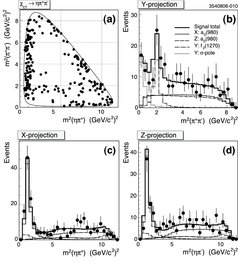
Figure 10: (a) Dalitz plot, (b)–(d) projections on the three mass squared combinations for $\chi_{c1}\to\pi^{+}\pi^{-}\eta$. The displayed fit projections are described in the text.

There are clear contributions from $a_{0}(980)^{\pm}\pi^{\mp}$ and $f_{2}(1270)\eta$ intermediate states, and significant accumulation of events at low $\pi^{+}\pi^{-}$ mass. Note that the $a_{0}(980)$ can contribute in two decay modes to the Dalitz plot. An isospin Clebsch-Gordan decomposition for this decay, given in Appendix VI, Equation 24, shows that amplitudes and strong phases of both charge-conjugated states should be equal. The overall amplitude normalization is arbitrary and we set $a_{a_{0}(980)^{+}}=a_{a_{0}(980)^{-}}=1$. All other fit components are defined relative to this choice.

Our initial fit to this mode includes only $a_{0}(980)^{\pm}\pi^{\mp}$ and $f_{2}(1270)\eta$ contributions, but has a vanishing probability of 0.1% for describing the data due to the accumulation of events at low $\pi^{+}\pi^{-}$ mass. To account for this we try $K^{0}_{S}$, $f_{0}(980)$, $\rho(770)$, and $\sigma$ resonances. Only the $\rho(770)$ and the $\sigma$ give high fit probability. However the decay $\chi_{c1}\to\rho(770)\eta$ is $C$-forbidden, and the low-mass distribution is not well represented by the $\rho(770)$, which only gives an acceptable fit due to its large width and the limited statistics of our sample. The $\sigma$ describes well the low $\pi^{+}\pi^{-}$ mass spectrum, and we describe the Dalitz plot with $a_{0}(980)^{\pm}\pi^{\mp}$, $f_{2}(1270)\eta$, and $\sigma\eta$ contributions. Table 7 gives the results of this fit, which has a probability to match the data of 66%. The angular distributions for $a_{0}(980)^{\pm}$ and $\sigma$ meson decays are uniform, and for $f_{2}(1270)$ are taken from Table 5 for quantum numbers $JjL=121$. We assume that a possible contribution from $L=3$ is small and it is neglected.

Table 6: Resonance parameters in the $\chi_{c1}\to\eta\pi^{+}\pi^{-}$ mode comparing their nominal value to fit values when individual resonance parameters are allowed to float.

Parameter	Nominal Value	When Floating
$m(a_{0}(980))$, MeV/c2	999	1002$\pm$18
$g_{\eta\pi}$, MeV/c2	620	637$\pm$49
$g_{K\bar{K}}$, MeV/c2	500	523$\pm$154
${\rm Re}(m_{\sigma})$, MeV/c2	470	511$\pm$28
${\rm Im}(m_{\sigma})$, MeV/c2	–220	–102$\pm$50

Table 7: Fit results for $\chi_{c1}\to\eta\pi^{+}\pi^{-}$ Dalitz plot analysis. The uncertainties are statistical and systematic. Allowing for interference among the resonances changes the fit fractions by as much as 20% in absolute terms as discussed in the text.

Mode	$a_{R}$	Fit Fraction (%)
$a_{0}(980)^{\pm}\pi^{\mp}$	1	$75.1\pm 3.5\pm 4.3$
$f_{2}(1270)\eta$	$0.103\pm 0.014\pm 0.005$	$14.4\pm 3.1\pm 1.9$
$\sigma\eta$	$0.41\pm 0.05\pm 0.10$	$10.5\pm 2.4\pm 1.2$

The systematic uncertainties shown in the table were obtained from variations to this nominal fit as discussed below. We allow the 2D-efficiency to vary with its polynomial coefficients constrained by the results of the fit to the simulated events; the mass of the $a_{0}(980)$ and its coupling constants are allowed to float, the parameters of the $\sigma$-pole are allowed to float, and we allow additional contributions from $\rho(770)\eta$, $f_{0}(980)\eta$, $K^{0}_{S}\eta$, and $\pi_{1}(1400)\pi$. The results of allowing the resonance parameters to float as compared to their fixed values used in the nominal fit are shown in Table 6. For the additional contributions we do not observe amplitudes that are significant and we limit their individual fit fractions to roughly less than 5% of the Dalitz plot. We note that with higher statistics this mode may offer one of the best measurements of the parameters of the $a_{0}(980)$. These results are consistent with the substructure analysis of this mode by BES BES .

The Dalitz plot for $\chi_{c1}\to K^{+}K^{-}\pi^{0}$ decay and its projections are shown in Figure 11, and

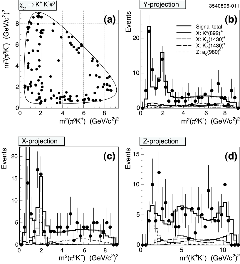
Figure 11: (a) Dalitz plot, (b)–(d) projections on the three mass squared combinations for $\chi_{c1}\to K^{+}K^{-}\pi^{0}$. The displayed fit projections are described in the text. The contribution from $\pi^{0}K^{-}$ resonances are not shown. They look similar to the $\pi^{0}K^{+}$ resonance components for the relevant projections.

for $\chi_{c1}\to\pi^{+}K^{-}K^{0}_{S}$ in Figure 12.

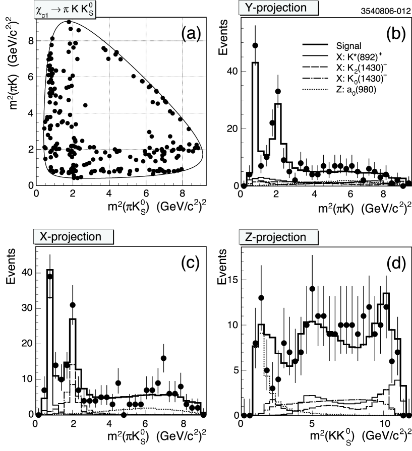
Figure 12: (a) Dalitz plot, (b)–(d) projections on the three mass squared combinations for $\chi_{c1}\to\pi^{+}K^{-}K^{0}_{S}$. The displayed fit projections are described in the text. The $\pi^{+}K^{-}$ resonances are not shown. They look similar to the $\pi^{+}K^{0}_{S}$ resonance components for the relevant projections.

We do a combined Dalitz plot analysis to these modes taking advantage of isospin symmetry. An isospin Clebsch-Gordan decomposition for these decays, described in Appendix VI, shows that these two Dalitz plots should have the same set of amplitudes for all $K^{*}\overline{K}$ and $a_{0}(980)\pi$ intermediate states. The relative factor $-\sqrt{2}$ between the two Dalitz plot amplitudes does not matter due to the individual normalization of their probability density functions. In the combined fit to these two Dalitz plots, we use the following constraints on the amplitudes: $a_{K^{*}}\equiv a_{K^{*+}}=a_{K^{*-}}=a_{K^{*0}}=a_{\overline{K}^{*0}}$, and $a_{a(980)}\equiv a_{a(980)^{+}}=a_{a(980)^{-}}=a_{a(980)^{0}}$. The overall amplitude normalization is arbitrary and we set $a_{K^{*}(892)}=1$.

Visual inspection shows apparent contributions from $K^{*}(892)^{\pm}K^{\mp}$, $K^{*}(892)^{0}K^{0}_{S}$, $K^{*}(1430)^{\pm}K^{\mp}$, $K^{*}(1430)^{0}K^{0}_{S}$, $a_{0}(980)^{0}\pi^{0}$, and $a_{0}(980)^{\pm}\pi^{\mp}$. It is not clear if the $K^{*}(1430)$ are $K^{*}_{0}$ or $K^{*}_{2}$, and many other $K\pi$ and $KK$ resonances can possibly contribute. The angular distribution for scalar resonance decays is always taken as uniform. The shape for $K^{*}(892)K$ is taken from Table 5 for quantum numbers $JjL=110$. We also modeled this contribution with the $JjL=112$ angular distribution with the difference taken as a systematic uncertainty. The shape for $K_{2}^{*}(1430)K$ is taken for quantum numbers $JjL=121$, with a possible contribution from $L=3$ ignored. Our best fit result is shown in Table 8, displaying

Table 8: Results of the combined fits to the $\chi_{c1}\to K^{+}K^{-}\pi^{0}$ and $\chi_{c1}\to\pi KK^{0}_{S}$ Dalitz plots. Allowing for interference among the resonances changes the fit fractions by as much as 15% in absolute terms as discussed in the text.

Mode	$a_{R}$	Fit Fraction (%)
$K^{*}(892)K$	1	$31.4\pm 2.2\pm 1.7$
$K^{*}_{0}(1430)K$	$3.8\pm 0.4\pm 0.2$	$30.4\pm 3.5\pm 3.7$
$K^{*}_{2}(1430)K$	$0.44\pm 0.06\pm 0.04$	$23.1\pm 3.4\pm 7.1$
$a_{0}(980)\pi$	$6.1\pm 0.6\pm 0.6$	$15.1\pm 2.7\pm 1.5$

statistical and systematic errors. This fit has a good probability of matching the data, 73%, and agrees with fits done to the separate Dalitz plots not taking advantage of isospin symmetry. The addition of a $\kappa K$ contribution does not improve the fit probability and the amplitude $a_{\kappa}$ is statistically significant only at the four standard deviation level. Similar behavior is noted for a non-resonant contribution. Systematic uncertainties are evaluated by observing deviations from the nominal fit as described above for the $\chi_{c1}\to\pi^{+}\pi^{-}\eta$ analysis. When systematics are taken into account neither the $\kappa K$ nor non-resonant contribution has a fit fraction significant at the three standard deviation level. Their individual contributions are limited to less than roughly 10% of the Dalitz plot. These observations are consistent with those by BES BES in the $\pi^{+}K^{-}K^{0}_{\rm S}$ mode.

While this model of the contributions to the Dalitz plots gives a good description of the data it is clearly incomplete. There should be interference among the resonances, which the simple approach of Equation 5 does not take into account. To quantify the effect of interference we have repeated the Dalitz analyses using a “quasi-coherent” (note that $\Omega_{R}^{2}$ is always positively-defined) sum of amplitudes with floating complex weighting factors instead of $a_{R}$. This causes the fit fractions to change by as much as $\sim$20% absolutely in the $\eta\pi\pi$ analysis and $\sim$15% absolutely in the $K\overline{K}\pi$ analysis. With more data a study of the $\chi_{c1}$ decay substructure taking into account the effect of $\chi_{c1}$ polarization, using the orientation of the $\chi_{c1}$ decay plane with respect to the $\chi_{c1}$ flight direction, in a partial wave analysis would be a complete description of these decays. The matrix element amplitudes should include the partial wave dependent angular distributions and interference effects among the resonances. See Ref. BES_PWA_formalism for appropriate prescriptions.

IV Summary

We have searched for and studied selected three-body hadronic decays of the $\chi_{c0}$, $\chi_{c1}$, and $\chi_{c2}$ produced in radiative decays of the $\psi(2S)$ in $e^{+}e^{-}$ collisions observed with the CLEO detector. Many of the channels covered in this analyses are observed or limited for the first time. Our observations and branching fraction limits are summarized in Table 4. In $\chi_{c1}\to\pi^{+}\pi^{-}\eta$ we have studied the resonant substructure using a Dalitz plot analysis simply modeling the resonance contributions as non-interfering amplitudes. Our results are summarized in Table 7. We observe clear signals for the $a_{0}(980)^{\pm}\pi^{\mp}$ and $f_{2}(1270)\eta$ intermediate states, and a low-mass $\pi^{+}\pi^{-}$ enhancement. Similarly for $\chi_{c1}\to K\overline{K}\pi$ our results are summarized in Table 8, assuming, based on isospin, that the $\pi KK^{0}_{S}$ and $K^{+}K^{-}\pi^{0}$ plots are identical. We observe $K^{*}(892)K$, $K^{*}_{2}(1430)K$ and likely $a_{0}(980)\pi$ contributions in the $K\overline{K}\pi$ Dalitz plots. Other conclusions about S-wave contributions are likely model-dependent.

V Acknowledgments

We gratefully acknowledge the effort of the CESR staff in providing us with excellent luminosity and running conditions. D. Cronin-Hennessy and A. Ryd thank the A.P. Sloan Foundation. This work was supported by the National Science Foundation, the U.S. Department of Energy, and the Natural Sciences and Engineering Research Council of Canada.

VI Appendix: Clebsch-Gordan decomposition for $\chi_{c1}$

In order to constrain amplitudes and phases in $\chi_{c1}$ decays we use a Clebsch-Gordan decomposition of the $\chi_{c1}$ (the state with $|I=0,I_{Z}=0\rangle$) for possible isospin subsystems:

$$\chi_{c1}\to(K\pi)_{I=1/2}{\overline{K}},$$ (10)

$$\chi_{c1}\to({\overline{K}}\pi)_{I=1/2}K,$$ (11)

$$\chi_{c1}\to(K{\overline{K}})_{I=1}\pi.$$ (12)

Below we use the Clebsch-Gordan decomposition rules, $|J,M\rangle=\sum_{f}c_{f}|m_{1},m_{2}\rangle_{f}$ from Ref. pdg .

VI.1 Clebsch-Gordan decomposition for $K^{*}\to K\pi$ decays

We assume that $K^{*}$ mesons with I=1/2 form two isodoublets: ($K^{*+}$, $K^{*0}$) and ($\overline{K}^{*0}$, $K^{*-}$) with ($I_{Z}=\frac{1}{2}$,$I_{Z}=-\frac{1}{2}$) respectively. The Clebsch-Gordan decomposition rules for $\mathbf{1\times\frac{1}{2}}$ isospin states are:

$$K^{*+}=\sqrt{\frac{2}{3}}\pi^{+}K^{0}-\sqrt{\frac{1}{3}}\pi^{0}K^{+},$$ (13)

$$K^{*0}=\sqrt{\frac{1}{3}}\pi^{0}K^{0}-\sqrt{\frac{2}{3}}\pi^{-}K^{+},$$ (14)

$$\overline{K}^{*0}=\sqrt{\frac{2}{3}}\pi^{+}K^{-}-\sqrt{\frac{1}{3}}\pi^{0}\overline{K}^{0},$$ (15)

$$K^{*-}=\sqrt{\frac{1}{3}}\pi^{0}K^{-}-\sqrt{\frac{2}{3}}\pi^{-}\overline{K}^{0}.$$ (16)

VI.2 Cases of $\chi_{c1}\to(K\pi)_{I=1/2}{\overline{K}}$ and $\chi_{c1}\to({\overline{K}}\pi)_{I=1/2}K$ decays

For $\chi_{c1}\to K^{*}\overline{K}$ and $\chi_{c1}\to\overline{K}^{*}K$ modes we use the $\mathbf{\frac{1}{2}\times\frac{1}{2}}$ rule:

$$\chi_{c1}=\frac{1}{\sqrt{2}}(K^{*+}K^{-}-K^{*0}\overline{K}^{0}),$$ (17)

$$\chi_{c1}=\frac{1}{\sqrt{2}}(\overline{K}^{*0}K^{0}-K^{*-}K^{+}).$$ (18)

Combining Equations 17 and 18 with Equations 13-16 we get

$$\chi_{c1}\sqrt{2}=\sqrt{\frac{2}{3}}\bigg{[}(\pi^{+}K^{0})K^{-}+(\pi^{-}K^{+})\overline{K}^{0}\bigg{]}-\sqrt{\frac{1}{3}}\bigg{[}(\pi^{0}K^{+})K^{-}+(\pi^{0}K^{0})\overline{K}^{0}\bigg{]},$$ (19)

$$\chi_{c1}\sqrt{2}=\sqrt{\frac{2}{3}}\bigg{[}(\pi^{+}K^{-})K^{0}+(\pi^{-}\overline{K}^{0})K^{+}\bigg{]}-\sqrt{\frac{1}{3}}\bigg{[}(\pi^{0}K^{-})K^{+}+(\pi^{0}\overline{K}^{0})K^{0}\bigg{]}.$$ (20)

Assuming charge symmetry the amplitudes in Equations 19 and 20 should be equal. From these equations we get the ratio of rates:

$$\Gamma(\chi_{c1}\to\pi^{+}K^{-}K^{0})/\Gamma(\chi_{c1}\to K^{+}K^{-}\pi^{0})=2,$$ (21)

$$\Gamma(\chi_{c1}\to\pi^{-}K^{+}\overline{K}^{0})/\Gamma(\chi_{c1}\to K^{+}K^{-}\pi^{0})=2,$$ (22)

or their sum

$$\Gamma(\chi_{c1}\to\pi^{+}K^{-}K^{0})+\Gamma(\chi_{c1}\to\pi^{-}K^{+}\overline{K}^{0})=4\cdot\Gamma(\chi_{c1}\to K^{+}K^{-}\pi^{0}).$$ (23)

VI.3 Case of $\chi_{c1}\to(K{\overline{K}})_{I=1}\pi$ decay

For $\chi_{c1}\to a\pi$ modes we use the $\mathbf{1\times 1}$ rule:

$$\chi_{c1}=\frac{1}{\sqrt{3}}(a^{+}\pi^{-}-a^{0}\pi^{0}+a^{-}\pi^{+})$$ (24)

For $a\to K{\overline{K}}$ we use the $\mathbf{\frac{1}{2}\times\frac{1}{2}}$ rules:

$$a^{+}=K^{+}\overline{K}^{0},$$ (25)

$$a^{0}=\frac{1}{\sqrt{2}}(K^{+}K^{-}+K^{0}\overline{K}^{0}),$$ (26)

$$a^{-}=K^{0}K^{-}.$$ (27)

Combining Equation 24 with Equations 25-27 we get

$$\chi_{c1}\sqrt{3}=(K^{+}\overline{K}^{0})\pi^{-}-\frac{1}{\sqrt{2}}\bigg{[}(K^{+}K^{-})\pi^{0}+(K^{0}\overline{K}^{0})\pi^{0}\bigg{]}+(K^{0}K^{-})\pi^{+}.$$ (28)

From Equation 28 we get the ratio of rates:

$$\Gamma(\chi_{c1}\to\pi^{+}K^{-}K^{0})/\Gamma(\chi_{c1}\to K^{+}K^{-}\pi^{0})=2,$$ (29)

$$\Gamma(\chi_{c1}\to\pi^{-}K^{+}\overline{K}^{0})/\Gamma(\chi_{c1}\to K^{+}K^{-}\pi^{0})=2,$$ (30)

or their sum

$$\Gamma(\chi_{c1}\to\pi^{+}K^{-}K^{0})+\Gamma(\chi_{c1}\to\pi^{-}K^{+}\overline{K}^{0})=4\cdot\Gamma(\chi_{c1}\to K^{+}K^{-}\pi^{0}).$$ (31)

VI.4 Consequences for Dalitz plot analysis

Comparing Equations 21-23 for intermediate states with $K^{*}$ and Equations 29-31 for intermediate states with $a(980)$, we note that they are identical. Thus observations of $\pi^{+}K^{-}K^{0}$ and charge conjugated $\pi^{-}K^{+}\overline{K}^{0}$ final states on the same Dalitz plot will yield the certain ratio between $K^{*}$ and $a(980)$ amplitudes for the $\pi KK^{0}_{S}$ Dalitz plot. The same ratio between $K^{*}$ and $a(980)$ amplitudes is expected for the $K^{+}K^{-}\pi^{0}$ Dalitz plot. This isospin analysis implies that these two Dalitz plots, $\pi KK^{0}_{S}$ and $K^{+}K^{-}\pi^{0}$, can be parametrized using a common set of parameters for each $K^{*}$ and $a(980)$ intermediate state. From Equations 19, 20 we can write equations between decay amplitudes with $K^{*}$ mesons

$${\rm for~{}}\pi KK^{0}_{S}:~{}~{}~{}a_{K^{*+}K^{-}\to K^{0}K\pi}=a_{K^{*-}K^{+}\to K^{0}K\pi}=a_{K^{*0}\overline{K}^{0}\to K^{0}K\pi}=a_{\overline{K}^{*0}K^{0}\to K^{0}K\pi}=$$

$${\rm for~{}}K^{+}K^{-}\pi^{0}:~{}~{}~{}~{}~{}=-\frac{1}{\sqrt{2}}a_{K^{*+}K^{-}\to K^{+}K^{-}\pi^{0}}=-\frac{1}{\sqrt{2}}a_{K^{*-}K^{+}\to K^{+}K^{-}\pi^{0}},$$ (32)

where the signs assume equal phases

$$\phi_{K^{*+}}=\phi_{K^{*-}}=\phi_{K^{*0}}=\phi_{\overline{K}^{*0}}.$$ (33)

Similar equations between amplitudes with $a_{0}(980)$ can be obtained from Equation 28

$${\rm for~{}}\pi KK^{0}_{S}:~{}~{}~{}a_{a(980)^{+}\pi^{-}\to\pi KK^{0}}=a_{a(980)^{-}\pi^{+}\to\pi KK^{0}}=$$

$${\rm for~{}}K^{+}K^{-}\pi^{0}:~{}~{}~{}=-\frac{1}{\sqrt{2}}a_{a(980)^{0}\pi^{0}\to K^{+}K^{-}\pi^{0}},$$ (34)

assuming equal phases

$$\phi_{a(980)^{+}}=\phi_{a(980)^{-}}=\phi_{a(980)^{0}}.$$ (35)

Equations 32 and 34 predict that the ratio of amplitudes between these two Dalitz plots is $-\sqrt{2}$. This relative factor does not matter, because each Dalitz plot is normalized separately. In the combined fit we ignore this $-\sqrt{2}$ factor between the amplitudes in the $\pi KK^{0}_{S}$ and $K^{+}K^{-}\pi^{0}$ Dalitz plots, and use common fit parameters for each of $K^{*}$ mesons and $a_{0}(980)$ intermediate states

$$a_{K^{*}}\equiv a_{K^{*+}}=a_{K^{*-}}=a_{K^{*0}}=a_{\overline{K}^{*0}},$$ (36)

$$a_{a(980)}\equiv a_{a(980)^{+}}=a_{a(980)^{-}}=a_{a(980)^{0}}.$$ (37)

In Sections VI.3 and VI.2 we have checked an isospin symmetry between $\pi KK^{0}$ and $K^{+}K^{-}\pi^{0}$ decays for two particular intermediate states. However, this symmetry is valid independently of how the amplitudes are decomposed into two-body sub-amplitudes, and thus should be valid for all points on the Dalitz plot.

References

- (1) N. Brambilla et al., CERN-2005-005 [hep-ph/0412158] is a comprehensive recent review of heavy quarkonium physics.
- (2) Q. Zhao, Phys. Rev. D 72, 074001 (2005).
- (3) S.B. Athar et al. (CLEO Collaboration), Phys. Rev. D 70, 112002 (2004).
- (4) M. Ablikim et al. (BES Collaboration), Phys. Rev. D 74, 072001 (2006).
- (5) G. Viehhauser et al., Nucl. Instrum. Methods A 462, 146 (2001).
- (6) R.A. Briere et al. (CESR-c and CLEO-c Taskforces, CLEO-c Collaboration), Cornell University, LEPP Report No. CLNS 01/1742 (2001) unpublished.
- (7) R. Brun et al., Geant 3.21, CERN Program Library Long Writeup W5013 (1993), unpublished.
- (8) G.S. Huang et al. (CLEO Collaboration), Phys. Rev. Lett. 95, 181801 (2005); T.E. Coan et al. (CLEO Collaboration), Phys. Rev. Lett. 95, 181802 (2005).
- (9) W.M. Yao et al., Journal of Physics G 33, 1 (2006) (PDG 2006).
- (10) V. Filippini, A. Fontana, and A. Rotondi, Phys. Rev. D 51, 2247 (1995).
- (11) S. Kopp et al. (CLEO Collaboration), Phys. Rev. D 63, 092001 (2001).
- (12) P. Rubin et al. (CLEO Collaboration), Phys. Rev. Lett. 93, 111801 (2004).
- (13) A. Abele et al. (Crystal Barrel Collaboration), Phys. Rev. D 57, 3860 (1998).
- (14) J.A. Oller, Phys. Rev. D 71, 054030 (2005).
- (15) B.S. Zou and D.V. Bugg, Eur. Phys. J. A16, 537 (2003).