Parametrization of Bose-Einstein Correlations and Reconstruction of the Source Function in Hadronic Z-boson Decays using the L3 Detector

Abstract

Bose-Einstein correlations of pairs of identical charged pions produced in hadronic Z decays are analyzed in terms of various parametrizations. A good description is achieved using a Lévy stable distribution in conjunction with a hadronization model having highly correlated configuration and momentum space, the $\tau$-model. Using these results, the source function is reconstructed.

I Introduction

In particle and nuclear physics, intensity interferometry provides a direct experimental method for the determination of sizes, shapes and lifetimes of particle-emitting sources (for reviews see  Gyulassy:1979 ; Boal:1990 ; Baym:1998 ; Wolfram:Zako2001 ; Tamas:HIP2002 ). In particular, boson interferometry provides a powerful tool for the investigation of the space-time structure of particle production processes, since Bose-Einstein correlations (BEC) of two identical bosons reflect both geometrical and dynamical properties of the particle radiating source.

Here we study BEC in hadronic $\mathrm{Z}$ decay. We investigate various static parametrizations in terms of the four-momentum difference, $Q=\sqrt{-(p_{1}-p_{2})^{2}}$ and find that none give an adequate description of the Bose-Einstein correlation function. However, within the framework of models assuming strongly correlated coordinate and momentum space a good description is achieved. We then reconstruct the complete space-time picture of the particle emitting source in hadronic Z decay.

The data used in the analysis were collected by the l3 detector l3:construction ; L3:Ecal_calib ; L3:Hcal ; L3:TEC ; l3:SMD at an $\mathrm{e^{+}}$$\mathrm{e^{-}}$  center-of-mass energy of $\sqrt{s}\simeq 91.2$ . Approximately 36 million like-sign pairs of well-measured charged tracks of about 0.8 million hadronic Z decays are used tamas .

We perform analyses on the complete sample as well as on two- and three-jet samples. The latter are found using calorimeter clusters with the Durham jet algorithm durham ; durham2 ; durham3 with a jet resolution parameter $y_{\mathrm{cut}}=0.006$. To determine the thrust axis of the event we also use calorimeter clusters.

II Bose-Einstein Correlation Function

The two-particle correlation function of two particles with four-momenta $p_{1}$ and $p_{2}$ is given by the ratio of the two-particle number density, $\rho_{2}(p_{1},p_{2})$, to the product of the two single-particle number densities, $\rho_{1}(p_{1})\rho_{1}(p_{2})$. Since we are here interested only in the correlation $R_{2}$ due to Bose-Einstein interference, the product of single-particle densities is replaced by $\rho_{0}(p_{1},p_{2})$, the two-particle density that would occur in the absence of Bose-Einstein correlations:

$$R_{2}(p_{1},p_{2})=\frac{\rho_{2}(p_{1},p_{2})}{\rho_{0}(p_{1},p_{2})}\;.$$ (1)

This $\rho_{2}$ is corrected for detector acceptance and efficiency using Monte Carlo events, to which a full detector simulation has been applied, on a bin-by-bin basis. An event mixing technique is used to construct $\rho_{0}$. This technique removes all correlations, not just Bose-Einstein. Hence, $\rho_{0}$ is corrected for this using Monte Carlo tamas .

Since the mass of the two identical particles of the pair is fixed to the pion mass, the correlation function is defined in six-dimensional momentum space. Since Bose-Einstein correlations can be large only at small four-momentum difference $Q$, they are often parametrized in this one-dimensional distance measure. There is no reason, however, to expect the hadron source to be spherically symmetric in jet fragmentation. Recent investigations have, in fact, found an elongation of the source along the jet axis L3_3D:1999 ; OPAL3D:2000 ; DELPHI2D:2000 ; ALEPH:2004 . While this effect is well established, the elongation is actually only about 20%, which suggests that a parametrization in terms of the single variable $Q$, may be a good approximation.

This is not the case in heavy-ion and hadron-hadron interactions, where BEC are found not to depend simply on $Q$, but on components of the momentum difference separately Tamas:HIP2002 ; Tamas;Lorstad:1996 ; NA22q ; Solz:thesis ; Solz:paper . However, in $\mathrm{e^{+}}$$\mathrm{e^{-}}$ annihilation at lower energy TASSO:1986 it has been observed that $Q$ is the appropriate variable. We checked this and confirm that this is indeed the case: We observe tamas that $R_{2}$ does not decrease when both $q^{2}=(\vec{p}_{1}-\vec{p}_{2})^{2}$ and $q_{0}^{2}=(E_{1}-E_{2})^{2}$ are large while $Q^{2}=q^{2}-q_{0}^{2}$ is small, but is maximal for $Q^{2}=q^{2}-q_{0}^{2}=0$, independent of the individual values of $q$ and $q_{0}$. The same is observed in a different decomposition: $Q^{2}=Q_{\mathrm{t}}^{2}+Q_{L,B}^{2}$, where $Q_{\mathrm{t}}^{2}=(\vec{p}_{\mathrm{t1}}-\vec{p}_{\mathrm{t2}})^{2}$ is the component transverse to the thrust axis and $Q_{L,B}^{2}=(p_{\mathrm{l1}}-p_{\mathrm{l2}})^{2}-(E_{1}-E_{2})^{2}$ combines the longitudinal momentum and energy differences. Again, $R_{2}$ is maximal along the line $Q=0$, as is shown in Fig. 1. This is observed both for two-jet and three-jet events. We conclude that a parametrization in terms of $Q$ can be considered a good approximation for the purposes of this article.

Figure 1: $R_{2}$ for two-jet events as function of the squares of the transverse momentum difference and the combination of longitudinal momentum difference and energy difference.

III Parametrizations of BEC

With a few assumptions GGLP:1960 ; Boal:1990 ; Tamas:HIP2002 , the two-particle correlation function, Eq. (1), is related to the Fourier transformed source distribution:

$$R_{2}(p_{1},p_{2})=\gamma\left[1+\lambda|\tilde{f}(Q)|^{2}\right]\left(1+\delta Q\right)\;,$$ (2)

where $f(x)$ is the (configuration space) density distribution of the source, and $\tilde{f}(Q)$ is the Fourier transform (characteristic function) of $f(x)$. The parameter $\gamma$ and the $(1+\delta Q)$ term have been introduced to parametrize possible long-range correlations not adequately accounted for in the reference sample, and the parameter $\lambda$ to account for several factors, such as the possible lack of complete incoherence of particle production and the presence of long-lived resonance decays if the particle emission consists of a small, resolvable core and a halo with experimentally unresolvable large length scales Bolz:1992hc ; Csorgo:1994in .

III.1 Gaussian distributed source

The simplest assumption is that the source has a symmetric Gaussian distribution, in which case $\tilde{f}(Q)=\exp\left(i\mu Q-\frac{(RQ)^{2}}{2}\right)$ and

$$R_{2}(Q)=\gamma\left[1+\lambda\exp\left(-(RQ)^{2}\right)\right]\left(1+\delta Q\right)\;.$$ (3)

A fit of Eq. (3) to the data results in an unacceptably low confidence level. The fit is particularly bad at low $Q$ values, as is shown in Fig. 2a for two-jet events and in Fig. 3a for three-jet events, from which we conclude that the shape of the source deviates from a Gaussian.

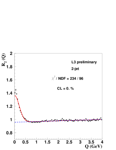
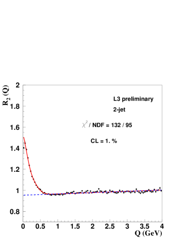
Figure 2: The Bose-Einstein correlation function $R_{2}$ for two-jet events with the result of a fit of (a) the Gaussian and (b) the Edgeworth parametrizations, Eqs. (3) and (4), respectively. The dashed line represents the long-range part of the fit, , $\gamma(1+\delta Q)$.

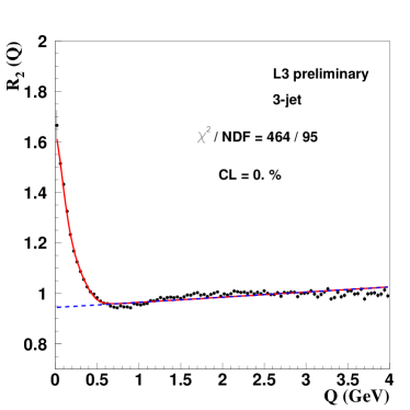
Figure 3: The Bose-Einstein correlation function $R_{2}$ for three-jet events with the result of a fit of (a) the Gaussian and (b) the Edgeworth parametrizations, Eqs. (3) and (4), respectively. The dashed line represents the long-range part of the fit, , $\gamma(1+\delta Q)$.

A model-independent way to study deviations from the Gaussian parametrization is to use Tamas:Moriond28 ; Tamas:Cracow1994 ; Tamas:HIP2002 the Edgeworth expansion Edgeworth about a Gaussian. Keeping only the first non-Gaussian term, we have

$$R_{2}(Q)=\gamma\left(1+\lambda\exp\left(-(RQ)^{2}\right)\left[1+\frac{\kappa}{3!}H_{3}(RQ)\right]\right)\left(1+\delta Q\right)\;,$$ (4)

where $\kappa$ is the third-order cumulant moment and $H_{3}(RQ)\equiv(\sqrt{2}RQ)^{3}-3\sqrt{2}RQ$ is the third-order Hermite polynomial. Note that the second-order cumulant corresponds to the radius $R$.

A fit of Eq. (4) to the two-jet data, shown in Fig. 2b, is indeed much better than the purely Gaussian fit. However, the confidence level is still marginal, and close inspection of the figure shows that the fit curve is systematically above the data in the region 0.6–1.2  and that the data for $Q\geq 1.5$  appear flatter than the curve, as is also the case for the purely Gaussian fit. Similar behavior is observed for three-jet events (Fig. 3b) and for all events.

III.2 Lévy distributed source

The symmetric Lévy stable distribution is characterized by three parameters: $x_{0}$, $R$, and $\alpha$. Its Fourier transform, $\tilde{f}(Q)$, has the following form:

$$\tilde{f}(Q)=\exp\left(iQx_{0}-\frac{|RQ|^{\alpha}}{2}\right)\;.$$ (5)

The index of stability, $\alpha$, satisfies the inequality $0<\alpha\leq 2$. The case $\alpha=2$ corresponds to a Gaussian source distribution with mean $x_{0}$ and standard deviation $R$. For more details, see, , Nolan .

Then $R_{2}$ has the following, relatively simple, form Tamas:Levy2004 :

$$R_{2}(Q)=\gamma\left[1+\lambda\exp\left(-(RQ)^{\alpha}\right)\right](1+\delta Q)\;.$$ (6)

From the fit of Eq. (6) to the two-jet data, shown in Fig. 4, it is clear that the correlation function is far from Gaussian: $\alpha=1.34\pm 0.04$. The confidence level, although improved compared to the fit of Eq. (3), is still unacceptably low, in fact worse than that for the Edgeworth parametrization. The same is true for three-jet events (Fig. 5) and for all events. The values of $\alpha$ are $1.39\pm 0.04$ for three-jet and $1.43\pm 0.03$ for all events, respectively.

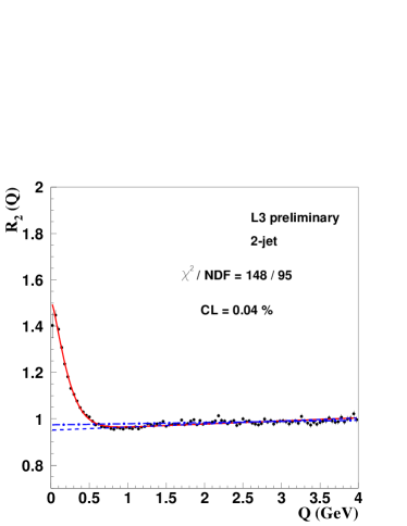
Figure 4: The Bose-Einstein correlation function $R_{2}$ for two-jet events. The curve corresponds to the fit of the symmetric Lévy parametrization, Eq. (6). The dashed line represents the long-range part of the fit, , $\gamma(1+\delta Q)$. The dot-dashed line represents a linear fit in the region $Q>1.5$ .

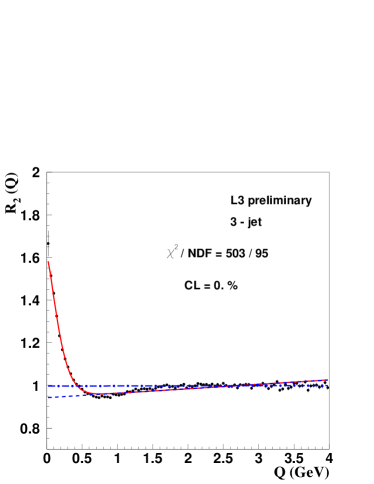
Figure 5: The Bose-Einstein correlation function $R_{2}$ for three-jet events. The curve corresponds to the fit of the symmetric Lévy parametrization, Eq. (6). The dashed line represents the long-range part of the fit, , $\gamma(1+\delta Q)$. The dot-dashed line represents a linear fit in the region $Q>1.5$ .

Both the symmetric Lévy parametrization and the Edgeworth parametrizations do a fair job of describing the region $Q<0.6\,\GeV$, but fail at higher $Q$. $R_{2}$ in the region $Q\geq 1.5\,\GeV$ is nearly constant ($\approx 1$). However, in the region 0.6–1.5  $R_{2}$ has a smaller value, dipping below unity , which is indicative of an anti-correlation. This is clearly seen in Figs. 4 and 5 by comparing the data in this region to an extrapolation of a linear fit, Eq. (6) with $\lambda=0$, in the region $Q\geq 1.5\,\GeV$. The inability to describe this dip in $R_{2}$ is the primary reason for the failure of both the Edgeworth and symmetric Lévy parametrizations.

III.3 Time dependence of the source

The parametrizations discussed so far, which have proved insufficient to describe the BEC, all assume a static source. The parameter $R$, representing the size of the source as seen in the rest frame of the pion pair, is a constant. It has, however, been observed that $R$ depends on the transverse mass, $m_{\mathrm{t}}=\sqrt{m^{2}+p_{\mathrm{t}}^{2}}=\sqrt{E^{2}-p_{z}^{2}}$, of the pions Smirnova:Nijm96 ; Dalen:Maha98 . It has been shown Bialas:1999 ; Bialas:2000 that this dependence can be understood if the produced pions satisfy, approximately, the (generalized) Bjorken-Gottfried condition Gottfried:1972 ; Bjorken:SLAC73 ; Bjorken:1973 ; Gottfried:1974 ; Low:1978 ; Bjorken:ISMD94 , whereby the four-momentum of a produced particle and the space-time position at which it is produced are linearly related:

$$x^{\mu}=dk^{\mu}\;.$$ (7)

Such a correlation between space-time and momentum-energy is also a feature of the Lund string model as incorporated in Jetset, which is very successful in describing detailed features of the hadronic final states of $\mathrm{e^{+}}$$\mathrm{e^{-}}$ annihilation.

In the previous section we have seen that BEC depend, at least approximately, only on $Q$ and not on its components separately. This is a non-trivial result. For a hydrodynamical type of source, on the contrary, BEC decrease when any of the relative momentum components is large Tamas:HIP2002 ; Tamas;Lorstad:1996 . Further, we have seen that $R_{2}$ in the region 0.6–1.5  dips below its values at higher $Q$.

A model which predicts such $Q$-dependence while incorporating the Bjorken-Gottfried condition is the so-called $\tau$-model, described below.

III.3.1 The $\tau$-model

A model of strongly correlated phase-space, known as the $\tau$-model Tamas;Zimanji:1990 , explains the experimentally found invariant relative momentum dependence of Bose-Einstein correlations in $\mathrm{e}^{+}\mathrm{e}^{-}$ reactions. This model also predicts a specific transverse mass dependence of $R_{2}$, that we subject to an experimental test here.

In this model, it is assumed that the average production point in the overall center-of-mass system, $\overline{x}=(\overline{t},\overline{r}_{x},\overline{r}_{y},\overline{r}_{z})$, of particles with a given four-momentum $k$ is given by

$$\overline{x}^{\mu}(k^{\mu})=dk^{\mu}\;.$$ (8)

In the case of two-jet events,

$$d=\tau/m_{\mathrm{t}}\;,$$ (9)

where $m_{\mathrm{t}}$ is the transverse mass and $\tau=\sqrt{\overline{t}^{2}-\overline{r}_{z}^{2}}$ is the longitudinal proper time . For isotropically distributed particle production, the transverse mass is replaced by the mass in Eq. (9), while for the case of three-jet events the relation is more complicated. The second assumption is that the distribution of $x^{\mu}(k^{\mu})$ about its average, $\delta_{\Delta}(x^{\mu}(k^{\mu})-\overline{x}^{\mu}(k^{\mu}))$, is narrower than the proper-time distribution. Then the emission function of the $\tau$-model is

$$S(x,k)=\int_{0}^{\infty}\mathrm{d}\tau H(\tau)\delta_{\Delta}(x-dk)\rho_{1}(k)\;,$$ (10)

where $H(\tau)$ is the longitudinal proper-time distribution, the factor $\delta_{\Delta}(x-dk)$ describes the strength of the correlations between coordinate space and momentum space variables and $\rho_{1}(k)$ is the experimentally measurable single-particle spectrum.

The two-pion distribution, $\rho_{2}(k_{1},k_{2})$, is related to $S(x,k)$, in the plane-wave approximation, by the Yano-Koonin formula Yano :

$$\rho_{2}(k_{1},k_{2}) = \int\mathrm{d}^{4}x_{1}\mathrm{d}^{4}x_{2}S(x_{1},k_{1})S(x_{2},k_{2})$$ (11)

$$\cdot\left(1+\cos\left(\left[k_{1}-k_{2}\right]\left[x_{1}-x_{2}\right]\right)\right)\;.$$

Approximating the function $\delta_{\Delta}$ by a Dirac delta function, the argument of the cosine becomes

$$(k_{1}-k_{2})(\bar{x}_{1}-\bar{x}_{2})=-0.5(d_{1}+d_{2})Q^{2}\;.$$ (12)

Then the two-particle Bose-Einstein correlation function is approximated by

$$R_{2}(k_{1},k_{2})=1+\lambda\mathrm{Re}\widetilde{H}^{2}\left(\frac{Q^{2}}{2\overline{m}_{\mathrm{t}}}\right)\;,$$ (13)

where $\widetilde{H}(\omega)=\int\mathrm{d}\tau H(\tau)\exp(i\omega\tau)$ is the Fourier transform of $H(\tau)$. Thus an invariant relative momentum dependent BEC appears. Note that $R_{2}$ depends not only on $Q$ but also on the average transverse mass of the two pions, $\overline{m}_{\mathrm{t}}$.

Since there is no particle production before the onset of the collision, $H(\tau)$ should be a one-sided distribution. We choose a one-sided Lévy distribution, which has the characteristic function Tamas:Levy2004 (for $\alpha\neq 1$)

$$\widetilde{H}(\omega)=\exp\left[-\frac{1}{2}\left(\Delta\tau|\omega|\right)^{\alpha}\left(1-i\,\mathrm{sign}(\omega)\tan\left(\frac{\alpha\pi}{2}\right)\right)+i\,\omega\tau_{0}\right]$$ (14)

where the parameter $\tau_{0}$ is the proper time of the onset of particle production and $\Delta\tau$ is a measure of the width of the proper-time distribution. For the special case $\alpha=1$, see, , Nolan . Using this characteristic function in Eq. (13) yields

$$R_{2}(Q,\overline{m}_{\mathrm{t}}) = \gamma\left[1+\lambda\cos\left(\frac{\tau_{0}Q^{2}}{\overline{m}_{\mathrm{t}}}+\tan\left(\frac{\alpha\pi}{2}\right)\left(\frac{\Delta\tau Q^{2}}{2\overline{m}_{\mathrm{t}}}\right)^{\!\alpha}\right)\right.$$ (15)

$$\cdot\left.\exp\left(-\left(\frac{\Delta\tau Q^{2}}{2\overline{m}_{\mathrm{t}}}\right)^{\!\alpha}\right)\right](1+\delta Q)\;.$$

III.3.2 The $\tau$-model for average $m_{\mathrm{t}}$

Before proceeding to fits of Eq. (15), we first consider a simplification of the equation obtained by assuming (a) that particle production starts immediately, , $\tau_{0}=0$, and (b) an average $m_{\mathrm{t}}$-dependence, which is implemented in an approximate way by defining an effective radius, $R=\sqrt{\Delta\tau/(2\overline{m}_{\mathrm{t}})}$. This results in:

$$R_{2}(Q)=\gamma\left[1+\lambda\cos\left[(R_{\mathrm{a}}Q)^{2\alpha}\right]\exp\left(-(RQ)^{2\alpha}\right)\right](1+\delta Q)\;,$$ (16)

where $R_{\mathrm{a}}$ is related to $R$ by

$$R_{\mathrm{a}}^{2\alpha}=\tan\left(\frac{\alpha\pi}{2}\right)R^{2\alpha}\;.$$ (17)

Fits of Eq. (16) are first performed with $R_{\mathrm{a}}$ as a free parameter. The fit results obtained, for two-jet, three-jet, and all events are listed in Table 1 and shown in Fig. 6 for two-jet events and in Fig. 7 for three-jet events. They have acceptable confidence levels, describing well the dip below unity in the 0.6–1.5  region, as well as the low-$Q$ peak.

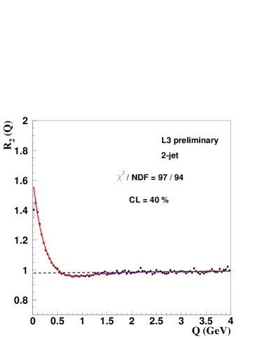
Figure 6: The Bose-Einstein correlation function $R_{2}$ for two-jet events. The curve corresponds to the fit of the one-sided Lévy parametrization, Eq. (16). The dashed line represents the long-range part of the fit, , $\gamma(1+\delta Q)$.

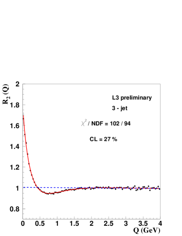
Figure 7: The Bose-Einstein correlation function $R_{2}$ for three-jet events. The curve corresponds to the fit of the one-sided Lévy parametrization, Eq. (16). The dashed line represents the long-range part of the fit, , $\gamma(1+\delta Q)$.

The fit parameters for the two-jet events satisfy Eq. (17). However, those for three-jet and all events do not. We note that the values of the parameters $\alpha$ and $R$ do not differ greatly between 2- and 3-jet samples, the most significant difference appearing to be nearly 3$\sigma$ for $\alpha$. However, these parameters are rather highly correlated (in the fit for all events, the correlation coefficients are $\rho(\lambda,R)=0.95$, $\rho(\lambda,\alpha)=-0.67$ and $\rho(R,\alpha)=-0.61$, which makes the simple calculation of the statistical significance of differences in the parameters unreliable.

Fit results imposing Eq. (17) are given in Table 2. For two-jet events, the values of the parameters are the same as in the fit with $R_{\mathrm{a}}$ free—only the uncertainties have changed. For three-jet and all events, the imposition of Eq. (17) results in values of $\alpha$ and $R$ closer to those for two-jet events, but the confidence levels are very bad, a consequence of incompatibility with Eq. (17), an incompatibility that is not surprizing given that Eq. (9) is only valid for two-jet events. Therefore, we only consider two-jet events in the remaining sections of this article.

Table 1: Results of fits of Eq. (16) for two-jet, three-jet, and all events. The uncertainties are only statistical.

parameter	2-jet		3-jet		all
$\alpha$	0.42$\;\pm\;$	0.02	0.35$\;\pm\;$	0.01	0.38$\;\pm\;$	0.01
$\lambda$	0.67$\;\pm\;$	0.03	0.84$\;\pm\;$	0.04	0.73$\;\pm\;$	0.02
$R$ (fm)	0.79$\;\pm\;$	0.04	0.89$\;\pm\;$	0.03	0.81$\;\pm\;$	0.03
$R_{\mathrm{a}}$ (fm)	0.59$\;\pm\;$	0.03	0.88$\;\pm\;$	0.04	0.81$\;\pm\;$	0.02
$\delta$	0.003$\;\pm\;$	0.002	–0.003$\;\pm\;$	0.002	0.003$\;\pm\;$	0.001
$\gamma$	0.979$\;\pm\;$	0.005	1.001$\;\pm\;$	0.005	0.997$\;\pm\;$	0.003
$\chi^{2}$/DoF	97/94		102/94		98/94
confidence level	40%		27%		37%

Table 2: Results of fits of Eq. (16) imposing Eq. (17) for two-jet, three-jet, and all events. The uncertainties are only statistical.

parameter	2-jet		3-jet		all
$\alpha$	0.42$\;\pm\;$	0.01	0.44$\;\pm\;$	0.01	0.45$\;\pm\;$	0.01
$\lambda$	0.67$\;\pm\;$	0.03	0.77$\;\pm\;$	0.04	0.69$\;\pm\;$	0.03
$R$ (fm)	0.79$\;\pm\;$	0.03	0.84$\;\pm\;$	0.04	0.79$\;\pm\;$	0.03
$\delta$	0.003$\;\pm\;$	0.001	0.010$\;\pm\;$	0.001	0.009$\;\pm\;$	0.001
$\gamma$	0.979$\;\pm\;$	0.005	0.972$\;\pm\;$	0.001	0.973$\;\pm\;$	0.001
$\chi^{2}$/DoF	97/95		174/95		175/95
confidence level	42%		$10^{-6}$		$10^{-6}$

III.3.3 The $\tau$-model with $m_{\mathrm{t}}$ dependence

Fits of Eq. (15) to the two-jet data are performed in several $m_{\mathrm{t}}$ intervals. The resulting fits are shown for several $m_{\mathrm{t}}$ intervals in Fig. 8, and the values of the parameters obtained in the fits are listed in Fig. 9. The quality of the fits is seen to be statistically acceptable and the fitted values of the model parameters, $\alpha$, $\tau_{0}$ and $\Delta\tau$, are stable and within errors independent of $m_{\mathrm{t}}$, confirming the expectation of the $\tau$-model. We conclude that the $\tau$-model with a one-sided Levy proper-time distribution describes the data with parameters $\tau_{0}\approx 0$ fm, $\alpha\approx 0.38\pm 0.05$ and $\Delta\tau\approx 3.5\pm 0.6$ fm. These values are consistent with the fit of Eq. (16) in the previous section, including the value of $R$, which, combined with the average value of $m_{\mathrm{t}}$ (0.563 ), corresponds to $\Delta\tau=3.5$ fm. Just as in the fit of Eq. (16), the parameters of the Lévy distribution are highly correlated. Typical values of the correlation coefficients are $\rho(\lambda,\Delta\tau)=0.95$, $\rho(\lambda,\alpha)=-0.67$ and $\rho(\Delta\tau,\alpha)=-0.9$.

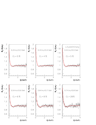
Figure 8: The results of fits of Eq. (15) to two-jet data for various intervals of $m_{\mathrm{t}}$.

Figure 9: The fit parameters from fits of Eq. (15) to two-jet data for various intervals of $m_{\mathrm{t}}$.

IV The emission function of two-jet events

Within the framework of the $\tau$-model, we now reconstruct the space-time picture of the emitting process for two-jet events. The emission function in configuration space, $S(x)$, is the proper time derivative of the integral over $k$ of $S(x,k)$, which in the $\tau$-model is given by Eq. (10). Approximating $\delta_{\Delta}$ by a Dirac delta function, we find

$$S(x)=\frac{\mathrm{d}^{4}n}{\mathrm{d}\tau\mathrm{d}^{3}r}=\left(\frac{m_{\mathrm{t}}}{\tau}\right)^{3}H(\tau)\rho_{1}\left(k=\frac{m_{\mathrm{t}}r}{\tau}\right)\;.$$ (18)

To simplify the reconstruction of $S(x)$ we assume that it can be factorized in the following way:

$$S(r,z,t)=I(r)G(\eta)H(\tau)\;,$$ (19)

where $I(r)$ is the single-particle transverse distribution, $G(\eta)$ is the space-time rapidity distribution of particle production, and $H(\tau)$ is the proper-time distribution. With the strongly correlated phase-space of the $\tau$-model, $\eta=y$ and $r=p_{\mathrm{t}}\tau/m_{\mathrm{t}}$. Hence,

$$G(\eta) = N_{y}(\eta)\;,$$ (20)

$$I(r) = \left(\frac{m_{\mathrm{t}}}{\tau}\right)^{\!3}N_{p_{\mathrm{t}}}(rm_{\mathrm{t}}/\tau)\;,$$ (21)

where $N_{y}$ and $N_{p_{\mathrm{t}}}$ are the single-particle inclusive rapidity and $p_{\mathrm{t}}$ distributions, respectively. The factorization of transverse and longitudinal distributions has been checked. The distribution of $p_{\mathrm{t}}$ is, to a good approximation, independent of the rapidity tamas .

Figure 10: The proper time distribution, $H(\tau)$, for $\alpha=0.4$, $\tau_{0}=0$ and $\Delta\tau=3.5$ fm.

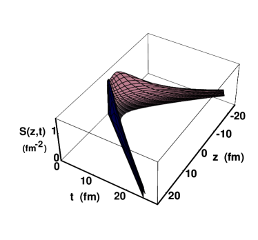
Figure 11: The temporal-longitudinal part of the source function normalized to the average number of pions per event.

With these assumptions and using $H(\tau)$ as obtained from the fit of Eq. (15) (shown in Fig. 10) together with the inclusive rapidity and $p_{\mathrm{t}}$ distributions tamas , the full emission function is reconstructed. Its integral over the transverse distribution is plotted in Fig. 11. It exhibits a “boomerang” shape with a maximum at low $t$ and $z$ but with tails reaching out to very large values of $t$ and $z$, a feature also observed in hadron-hadron NA22emiss and heavy ion collisions HIemiss:Ster .

The transverse part of the emission function is obtained by integrating over $z$ and azimuthal angle. Figure 12 shows the transverse part of the emission function for various proper times. Particle production starts immediately, increases rapidly and decreases slowly. A ring-like structure, similar to the expanding, ring-like wave created by a pebble in a pond, is observed. These pictures together form a movie that ends in about 3.5 fm, making it the shortest movie ever made of a process in nature. An animated gif file covering the first 0.3 fm (10^-24 sec) is available tamas_movie .

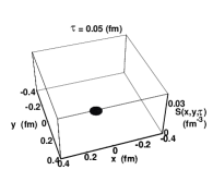
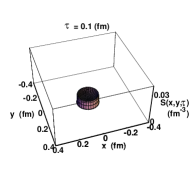
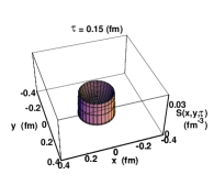
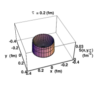
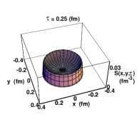
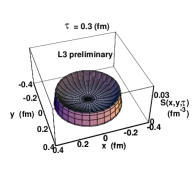
Figure 12: The transverse source function normalized to the average number of pions per event for various proper times.

V Discussion

BEC of all events as well as two- and three-jet events are observed to be well-described by a Lévy parametrization incorporating strong correlations between configuration- and momentum-space. A Lévy distribution arises naturally from a fractal, or from a random walk or anomalous diffusion metzler , and the parton shower of the leading log approximation of QCD is a fractal Dahlqvist:1989yc ; Gustafson:1990qi ; Gustafson:1991ru . In this case, the Lévy index of stability is related to the strong coupling constant, $\as$, byalphasLevy ; alphasLevy:arx

$$\as=\frac{2\pi}{3}\alpha^{2}\;.$$ (22)

Assuming (generalized) local parton hadron duality Azimov:lphd ; Azimov:lphd1 ; genlphd , one can expect that the distribution of hadrons retains the features of the gluon distribution. For the value of $\alpha$ found in fits of Eq. (16) we find $\as=0.37\pm 0.04$ for two-jet events, This is a reasonable value for a scale of 1–2 , which is where the production of hadrons takes place. For comparison, from $\tau$ decay, $\as(m_{\tau}\approx 1.8\,\GeV)=0.35\pm 0.03$ PDG:2004 .

It is of particular interest to point out the $m_{\mathrm{t}}$ dependence of the “width” of the source. In Eq. (15) the parameter associated with the width is $\Delta\tau$. Note that it enters Eq. (15) as $\Delta\tau Q^{2}/\overline{m}_{\mathrm{t}}$. In a Gaussian parametrization the radius $R$ enters the parametrization as $R^{2}Q^{2}$. Our observance that $\Delta\tau$ is independent of $\overline{m}_{\mathrm{t}}$ thus corresponds to $R\propto 1/\sqrt{\overline{m}_{\mathrm{t}}}$ and can be interpreted as confirmation of the observance Smirnova:Nijm96 ; Dalen:Maha98 of such a dependence of the Gaussian radii in 2- and 3-dimensional analyses of Z decays. The lack of dependence of all the parameters of Eq. (15) on the transverse mass is in accordance with the $\tau$-model.

Using the BEC fit results and the $\tau$-model, the emission function of two-jet events is reconstructed. Particle production begins immediately after collision, increases rapidly and then decreases slowly, occuring predominantly close to the light cone. In the transverse plane a ring-like structure expands outwards, which is similar to the picture in hadron-hadron interactions but unlike that of heavy ion collisions.

References

- (1) M. Gyulassy, S.K. Kauffmann and Lance W. Wilson, Phys. Rev. C20 (1979) 2267–2292.
- (2) David H. Boal, Claus-Konrad Gelbke and Byron K. Jennings, Rev. Mod. Phys. 62 (1990) 553–602.
- (3) Gordon Baym, Acta Phys. Pol. B29 (1998) 1839–1884.
- (4) W. Kittel, Acta Phys. Pol. B32 (2001) 3927–3972.
- (5) T. Csörgő, Heavy Ion Physics 15 (2002) 1–80.
- (6) L3 Collab., B. Adeva \etal, Nucl. Inst. Meth. A 289 (1990) 35–102.
- (7) J.A. Bakken \etal, Nucl. Inst. Meth. A 275 (1989) 81–88.
- (8) O. Adriani \etal, Nucl. Inst. Meth. A 302 (1991) 53–62.
- (9) K. Deiters \etal, Nucl. Inst. Meth. A 323 (1992) 162–168.
- (10) M. Acciarri \etal, Nucl. Inst. Meth. A 351 (1994) 300–312.
- (11) Tamás Novák, Ph.D. thesis, Radboud Univ. Nijmegen, in preparation.
- (12) Yu.L. Dokshitzer, Contribution cited in Report of the Hard QCD Working Group, Proc. Workshop on Jet Studies at LEP and HERA, Durham, Dec. 1990, J. Phys. G17 (1991) 1537.
- (13) S. Catani \etal, Phys. Lett. B269 (1991) 432–438.
- (14) S. Bethke \etal, Nucl. Phys. B370 (1992) 310–334.
- (15) L3 Collab., M. Acciarri \etal, Phys. Lett. B458 (1999) 517–528.
- (16) OPAL Collab., G. Abbiendi \etal, Eur. Phys. J. C16 (2000) 423–433.
- (17) DELPHI Collab., P. Abreu \etal, Phys. Lett. B471 (2000) 460–470.
- (18) ALEPH Collab., A. Heister \etal, Eur. Phys. J. C36 (2004) 147–159.
- (19) T. Csörgő and B. Lörstadt, Phys. Rev. C54 (1996) 1390–1403.
- (20) NA22 Collab., N.M. Agababyan \etal, Z. Phys. C71 (1996) 405–414.
- (21) Ron A. Solz, Two-Pion Correlation Measurements for 14.6A\GeV/ 28Si+X and 11.6A\GeV/ 197Au+Au, Ph.D. thesis, Massachusetts Inst. of Technology., 1994.
- (22) E-802 Collab., L. Ahle \etal, Phys. Rev. C66 (2002) 054906–1–15.
- (23) TASSO Collab., M. Althoff \etal, Z. Phys. C30 (1986) 355–369.
- (24) Gerson Goldhaber, Sulamith Goldhaber, Wonyong Lee and Abraham Pais, Phys. Rev. 120 (1960) 300–312.
- (25) J. Bolz \etal, Phys. Rev. D47 (1993) 3860–3870.
- (26) T. Csörgő, B. Lörstad and J. Zimányi, Z. Phys. C71 (1996) 491–497.
- (27) T. Csörgő and S. Hegyi, in Proc. XXVIIIth Rencontres de Moriond, ed. Étienne Augé and J. Trân Thanh Vân, (Editions Frontières, Gif-sur-Yvette, France, 1993), p. 635.
- (28) T. Csörgő, in Proc. Cracow Workshop on Multiparticle Production, ed. A. Białas \etal, (World Scientific, Singapore, 1994), p. 175.
- (29) F.Y. Edgeworth, Trans. Cambridge Phil. Soc. 20 (1905) 36, see also, \eg, Harald Cramér, Mathematical Methods of Statistics, (Princeton Univ. Press, 1946).
-
(30)
J.P. Nolan,
Stable distributions: Models for Heavy Tailed Data, 2005,
http://academic2.american.edu/jpnolan/
stable/CHAP1.PDF. - (31) T. Csörgő, S. Hegyi and W.A. Zajc, Eur. Phys. J. C36 (2004) 67–78.
- (32) B. Lörstad and O.G. Smirnova, in Proc. 7th Int. Workshop on Multiparticle Production “Correlations and Fluctuations”, ed. R.C. Hwa \etal, (World Scientific, Singapore, 1997), p. 42.
- (33) J.A. van Dalen, in Proc. 8th Int. Workshop on Multiparticle Production “Correlations and Fluctuations ’98: From QCD to Particle Interferometry”, ed. T. Csörgő \etal, (World Scientific, Singapore, 1999), p. 37.
- (34) A. Białas and K. Zalewski, Acta Phys. Pol. B30 (1999) 359–367.
- (35) A. Białas \etal, Phys. Rev. D62 (1999) 114007–1–7.
- (36) K. Gottfried, Acta Phys. Pol. B3 (1972) 769.
- (37) J.D. Bjorken, in Proc. Summer Inst. on Particle Physics, Vol. 1, (SLAC-R-167, 1973), pp. 1–34.
- (38) J.D. Bjorken, Phys. Rev. D7 (1973) 282–283.
- (39) K. Gottfried, Phys. Rev. Lett. 32 (1974) 957–961.
- (40) F.E. Low and K. Gottfried, Phys. Rev. D17 (1978) 2487–2491.
- (41) J.D. Bjorken, in Proc. XXIV Int. Symp. on Multiparticle Dynamics, ed. A. Giovannini \etal, (World Scientific, Singapore, 1995), p. 579.
- (42) T. Csörgő and J. Zimányi, Nucl. Phys. A517 (1990) 588–598.
- (43) F.B. Yano and S.E. Koonin, Phys. Lett. B78 (1978) 556–559.
- (44) NA22 Collab., N.M. Agababyan \etal, Phys. Lett. B422 (1998) 359–368.
- (45) A. Ster, T. Csörgő and B. Lörstad, Nucl. Phys. A661 (1999) 419–422.
-
(46)
T. Novák,
http://www.hef.kun.nl/novakt/movie/movie.
gif. - (47) R. Metzler and J. Klafter, Phys. Rep. 339 (2000) 1–77.
- (48) P. Dahlqvist, B. Andersson and G. Gustafson, Nucl. Phys. B328 (1989) 76.
- (49) G. Gustafson and A. Nilsson, Nucl. Phys. B355 (1991) 106.
- (50) G. Gustafson and A. Nilsson, Z. Phys. C52 (1991) 533.
- (51) T. Csörgő \etal, Acta Phys. Pol. B36 (2005) 329–337.
- (52) T. Csörgő \etal, Bose-Einstein or HBT correlation signature of a second order QCD phase transition, 2005, http://arXiv.org/abs/nucl-th/0512060.
- (53) Ya.I. Azimov \etal, Z. Phys. C27 (1985) 65–72.
- (54) Ya.I. Azimov \etal, Z. Phys. C31 (1986) 213–218.
- (55) L. Van Hove and A. Giovannini, Acta Phys. Pol. B19 (1988) 931–946.
- (56) Particle Data Group, S. Eidelman \etal, Phys. Lett. B592 (2004) 1–1109.