Measurement of the $t\overline{t}~{}$ production cross section in $p\bar{p}$ collisions at $\sqrt{s}$ = 1.96 TeV using secondary vertex $b$ tagging

Abstract

We report a new measurement of the $t\overline{t}$ production cross section in $p\bar{p}$ collisions at a center-of-mass energy of 1.96 TeV using events with one charged lepton (electron or muon), missing transverse energy, and jets. Using $425\;\rm pb^{-1}$ of data collected using the D0 detector at the Fermilab Tevatron Collider, and enhancing the $t\overline{t}$ content of the sample by tagging $b$ jets with a secondary vertex tagging algorithm, the $t\overline{t}$ production cross section is measured to be:

$$\sigma_{p\overline{p}\rightarrow t\overline{t}+X}=6.6\pm 0.9\>{\rm(stat+syst)}\>\pm 0.4\>{\rm(lum)}\>{\rm pb}.$$

This cross section is the most precise D0 measurement to date for $t\overline{t}$ production and is in good agreement with standard model expectations.

I Introduction

The top quark was discovered at the Fermilab Tevatron Collider in 1995 topdiscoveryI ; topdiscoveryII and completes the quark sector of the three-generation structure of the standard model (SM). It is the heaviest known elementary particle with a mass approximately 40 times larger than that of the next heaviest quark, the bottom quark. It differs from the other quarks not only by its much larger mass, but also by its lifetime which is too short to build hadronic bound states. The top quark is one of the least-studied components of the SM, and the Tevatron, with a center of mass energy of $\sqrt{s}=1.96\;\rm TeV$, is at present the only accelerator where it can be produced. The top quark plays an important role in the discovery of new particles, as the Higgs boson coupling to the top quark is stronger than to all other fermions. Understanding the signature and production rate of top quark pairs is a crucial ingredient in the discovery of new physics beyond the SM. In addition, it lays the ground for measurements of top quark properties at D0.

The top quark is pair-produced in $p\overline{p}$ collisions through quark-antiquark annihilation and gluon-gluon fusion. The Feynman diagrams of the leading order (LO) subprocesses are shown in Fig. 1. At Tevatron energies, the $q\bar{q}\rightarrow t\bar{t}$ process dominates, contributing 85% of the cross section. The $gg\rightarrow t\bar{t}$ process contributes the remaining 15%.

Figure 1: Leading order Feynman diagrams for the production of $t\overline{t}$ pairs at the Tevatron.

The total top quark pair production cross section for a hard scattering process initiated by a $p\overline{p}$ collision at the center of mass energy $\sqrt{s}$ is a function of the top quark mass $m_{t}$ and can be expressed as

$$\sigma^{p\overline{p}\rightarrow t\overline{t}+X}(s,m_{t})=\sum\limits_{i,j=q,\overline{q},g}\int dx_{i}dx_{j}f_{i}(x_{i},\mu^{2})$$ (1)

$$\times\overline{f_{j}}(x_{j},\mu^{2})\hat{\sigma}^{ij\rightarrow t\overline{t}}(\rho,m_{t}^{2},\alpha_{s}(\mu^{2}),\mu^{2}).$$

The summation indices $i$ and $j$ run over the light quarks and gluons, $x_{i}$ and $x_{j}$ are the momentum fractions of the partons involved in the $p\overline{p}$ collision, and $f_{i}(x_{i},\mu^{2})$ and $\overline{f_{j}}(x_{j},\mu^{2})$ are the parton distribution functions (PDFs) for the proton and the antiproton, respectively. $\hat{\sigma}^{ij\rightarrow t\overline{t}}(\rho,m_{t}^{2},\alpha_{s}(\mu^{2}),\mu^{2})$ is the total short distance cross section at $\hat{s}\equiv x_{i}\cdot x_{j}\cdot s$, and is computable as a perturbative expansion in $\alpha_{s}$. The renormalization and factorization scales are chosen to be the same parameter $\mu$, with dimensions of energy, and $\rho\equiv\frac{4m_{t}^{2}}{\hat{s}}$. The theoretical uncertainties on the $t\overline{t}$ cross section arise from the choice of $\mu$ scale, PDFs, and $\alpha_{s}$. For the most recent calculations of the top quark pair production cross section, the parton-level cross sections include the full NLO matrix elements nason , and the resummation of leading (LL) catani and next-to-leading (NLL) soft logarithms bonciani appearing at all orders of perturbation theory. For a top quark mass of $175\;\rm GeV$, the predicted SM $t\overline{t}$ production cross section is $6.7^{+0.7}_{-0.9}\;\rm pb^{-1}$ theoxsec . Deviations of the measured cross section from the theoretical prediction could indicate effects beyond QCD perturbation theory. Explanations might include substantial non-perturbative effects, new production mechanisms, or additional top quark decay modes beyond the SM. Previous measurements CDFRun2 ; D0Run2 ; topoprd ; dileptonpaper show good agreement with the theoretical expectation.

Within the SM, the top quark decays via the weak interaction to a $W$ boson and a $b$ quark, with a branching fraction $Br(t\rightarrow Wb)>$ 0.998 pdg . The $t\overline{t}$ pair decay channels are classified as follows: the dilepton channel, where both $W$ bosons decay leptonically into an electron or a muon ($ee$, $\mu\mu$, $e\mu$); the $l$+jets channel, where one of the $W$ bosons decays leptonically and the other hadronically ($e$+jets, $\mu$+jets); and the all-jets channel, where both $W$ bosons decay hadronically. A fraction of the $\tau$ leptons decays leptonically to an electron or a muon, and two neutrinos. These events have the same signature as events in which the $W$ boson decays directly to an electron or a muon and are treated as part of the signal in the $l$+jets channel. In addition, dilepton events in which one of the leptons is not identified are also treated as part of the signal in the $l$+jets channel. Two $b$ quarks are present in the final state of a $t\overline{t}$ event which distinguishes it from most of the background processes. As a consequence, identifying the bottom flavor of the corresponding jet can be used as a selection criteria to isolate the $t\overline{t}$ signal.

This article presents a new measurement thesisGustavo of the $t\overline{t}$ production cross section in the $l$+jets channel. The events contain one charged lepton ($e$ or $\mu$) from a leptonic $W$ boson decay with high transverse momentum, missing transverse energy ($\not\!\!E_{T}$) from the neutrino emitted in the $W$ boson decay, two $b$ jets from the hadronization of the $b$ quarks, and two non-$b$ jets ($u$, $d$, $s$, or $c$) from the hadronic $W$ decay; additional jets are possible due to initial (ISR) and final state radiation (FSR). $b$ jets in the event are identified by explicitly reconstructing secondary vertices; the addition of the silicon microstrip tracker to the upgraded detector in Run II made this technique feasible for the first time at D0.

This paper is organized as follows: the Run II D0 detector is described in Section II with special emphasis on those aspects that are relevant to this analysis. The trigger and event reconstruction/particle identification techniques used to select events that contain an electron or muon and jets are discussed in Sec. III and IV. The methods used to simulate $t\overline{t}$ and background events are explained in Sec. V. A data-based method that is used to estimate the contribution from instrumental and physics backgrounds to the $l$+jets sample is presented in Sec. VI. The methods used to estimate the efficiency and fake rate of the $b$ tagging algorithm are explained in Sec. VII. The means for estimating all contributions to the $l$+jets sample after tagging are detailed in Sec. VIII. Finally, the description of the method used to extract the cross section is presented in Sec. IX. The simulation of $W$ boson events produced in association with jets is detailed in Appendix A, and the handling of the statistical uncertainty on the cross section extraction procedure is explained in Appendix B.

II The D0 Detector

The D0 detector d0_nim is a multi-purpose apparatus designed to study $p\overline{p}$ collisions at high energies. It consists of three major subsystems. At the core of the detector, a magnetized tracking system precisely records the trajectories of charged particles and measures their transverse momenta. A hermetic, finely-grained uranium and liquid argon calorimeter measures the energies of electromagnetic and hadronic showers. A muon spectrometer measures the momenta of muons.

II.1 Coordinate System

The Cartesian coordinate system used for the D0 detector is right-handed with the $z$ axis parallel to the direction of the protons, the $y$ axis vertical, and the $x$ axis pointing out from the center of the accelerator ring. A particular reformulation of the polar angle $\theta$ is given by the pseudorapidity defined as $\eta\equiv-\ln({\tan{\theta/2}})$. In addition, the momentum vector projected onto a plane perpendicular to the beam axis (transverse momentum) is defined as $p_{T}=p\cdot\mathrm{sin}\theta$. Depending on the choice of the origin of the coordinate system, the coordinates are referred to as physics coordinates ($\phi$, $\eta$) when the origin is the reconstructed vertex of the interaction, or as detector coordinates ($\phi_{\text{det}}$, $\eta_{\text{det}}$) when the origin is chosen to be the center of the D0 detector.

II.2 Luminosity Monitor

The Tevatron luminosity at the D0 interaction region is measured from the rate of inelastic $p\overline{p}$ collisions observed by the luminosity monitor (LM). The LM consists of two arrays of twenty-four plastic scintillator counters with photomultiplier readout. The arrays are located in front of the forward calorimeters at $z=\pm 140\;\rm cm$ and occupy the region between the beam pipe and the forward preshower detector. The counters are $15\;\rm cm$ long and cover the pseudorapidity range $2.7<|\eta_{\text{det}}|<4.4$. The uncertainty on the luminosity is currently estimated to be 6.1% lumi .

II.3 The Central Tracking System

The purpose of the central tracking system nim-tracker is to measure the momenta, directions, and signs of the electric charges for charged particles produced in a collision. The silicon microstrip tracker (SMT) is located closest to the beam pipe and allows for an accurate determination of impact parameters and identification of secondary vertices. The length of the interaction region ($\sigma\approx 25$ cm) led to the design of barrel modules interspersed with disks, and assemblies of disks in the forward and backward regions. The barrel detectors measure primarily the $r$-$\phi$ coordinate, and the disk detectors measure $r$-$z$ as well as $r$-$\phi$. The detector has six barrels in the central region; each barrel has four silicon readout layers, each composed of two staggered and overlapping sub-layers. Each barrel is capped at high $|z|$ with a disk of twelve double-sided wedge detectors, called an F-disk. In the far forward and backward regions, a unit consisting of three F-disks and two large-diameter H-disks provides tracking at high $|\eta_{\text{det}}|<3.0$. Ionized charge is collected by $p$ or $n$ type silicon strips of pitch between $50$ and $150~{}\mu\rm m$ that are used to measure the position of the hits. The axial hit resolution is of the order of $10~{}\mu\rm m$, the $z$ hit resolution is $35~{}\mu\rm m$ for $90^{\circ}$ stereo and $450~{}\mu\rm m$ for $2^{\circ}$ stereo detector modules.

Surrounding the SMT is the central fiber tracker (CFT), which consists of $835~{}\mu\rm m$ diameter scintillating fibers mounted on eight concentric support cylinders and occupies the radial space from 20 to 52 cm from the center of the beam pipe. The two innermost cylinders are 1.66 m long, and the outer six cylinders are 2.52 m long. Each cylinder supports one doublet layer of fibers oriented along the beam direction and a second doublet layer at a stereo angle of alternating $+3^{\circ}$ and $-3^{\circ}$. In each doublet the two layers of fibers are offset by half a fiber width to provide improved coverage. The CFT has a cluster resolution of about $100~{}\mu\rm m$ per doublet layer.

The momenta of charged particles are determined from their curvature in the 2 T magnetic field provided by a 2.7 m long superconducting solenoid magnet magnets . The superconducting solenoid, a two layer coil with mean radius 60 cm, has a stored energy of 5 MJ and operates at $10$ K. Inside the tracking volume, the magnetic field along the trajectory of any particle reaching the solenoid is uniform within 0.5%. The uniformity is achieved in the absence of a field-shaping iron return yoke by using two grades of conductor. The superconducting solenoid coil plus cryostat wall has a thickness of about 0.9 radiation lengths in the central region of the detector.

Hits from both tracking detectors are combined to reconstruct tracks. The measured momentum resolution of the tracker can be parameterized as $\frac{\sigma(1/p_{T})}{1/p_{T}}=\sqrt{\frac{(0.003p_{T})^{2}}{L^{4}}+\frac{0.026^{2}}{L\sin\theta}}$, with the first term accounting for the measurement uncertainty of the individual hits in the tracker, and the second term for the multiple scattering. In the expression above, $p_{T}$ is the particle’s transverse momentum (in GeV), and $L$ is the normalized track bending lever arm. $L$ is equal to 1 for tracks with $|\eta|<1.62$ and equal to $\frac{\tan\theta}{\tan\theta^{\prime}}$ otherwise. $\theta^{\prime}$ represents the angle at which the track exits the tracker.

II.4 The Calorimeter System

The uranium/liquid-argon sampling calorimeters constitute the primary system used to identify electrons, photons, and jets. The system is subdivided into the central calorimeter (CC) covering roughly $|\eta_{\text{det}}|<1$ and two end calorimeters (EC) extending the coverage to $|\eta_{\text{det}}|\approx 4$. Each calorimeter contains an electromagnetic (EM) section closest to the interaction region, followed by fine and coarse hadronic sections with modules that increase in size with the distance from the interaction region. Each of the three calorimeters is located within a cryostat that maintains the temperature at approximately $80$ K. The EM sections use thin 3 or 4 mm plates made from nearly pure depleted uranium. The fine hadronic sections are made from 6 mm thick uranium-niobium alloy. The coarse hadronic modules contain relatively thick 46.5 mm plates of copper in the CC and stainless steel in the EC. The intercryostat region, between the CC and the EC calorimeters, contains additional layers of sampling, the scintillator-based intercryostat detector, to improve the energy resolution. The CC and EC contain approximately seven and nine interaction lengths of material respectively, ensuring containment of nearly all particles except high $p_{T}$ muons and neutrinos.

The preshower detectors are designed to improve the identification of electrons and photons and to correct for their energy losses in the solenoid during offline event reconstruction. The central preshower detector (CPS) is located in the 5 cm gap between the solenoid and the CC, covering the region $|\eta_{\text{det}}|<$ 1.3. The two forward preshower detectors (FPSs) are attached to the faces of the ECs and cover the region 1.5 $<|\eta_{\text{det}}|<$ 2.5. The relative momentum resolution for the calorimeter system is measured in data and found to be $\sigma(p_{T})/p_{T}\approx 13\%$ for $50\;\rm GeV$ jets in the CC and $\sigma(p_{T})/p_{T}\approx 12\%$ for $50\;\rm GeV$ jets in the ECs. The energy resolution for electrons in the CC is $\sigma(E)/E\approx 15\%\sqrt{E}\oplus 4\%$.

II.5 The Muon System

The muon system nim-muons is the outermost part of the D0 detector. It surrounds the calorimeters and serves to identify and trigger on muons and to provide crude measurements of momentum and charge. It consists of a system of proportional drift tubes (PDTs) that cover the region of $|\eta_{\text{det}}|<1.0$ and mini drift tubes (MDTs) that extend coverage to $|\eta_{\text{det}}|\approx 2.0$. Scintillation counters are used for triggering and for cosmic and beam-halo muon rejection. Toroidal magnets and special shielding complete the muon system. Each subsystem has three layers, with the innermost layer located between the calorimeter and the iron of the toroid magnet. The two remaining layers are located outside the iron. In the region directly below the CC, only partial coverage by muon detectors is possible to accomodate the support structure for the detector and the readout electronics. The average energy loss of a muon is $1.6\;\rm GeV$ in the calorimeter and $1.7\;\rm GeV$ in the iron; the momentum measurement is corrected for this energy loss. The average momentum resolution for tracks that are matched to the muon and include information from the SMT and the CFT is measured to be $\sigma(p_{T})=0.02\oplus 0.002p_{T}$ (with $p_{T}$ in GeV).

III Triggers

The trigger system is a three-tiered pipelined system. The first stage (Level 1) is a hardware trigger that consists of a framework built of field programmable gate arrays (FPGAs) which take inputs from the luminosity monitor, calorimeter, central fiber tracker, and muon system. It makes a decision within $4.2~{}\mu\rm s$ and results in a trigger accept rate of about $2\;\rm kHz$. In the second stage (Level 2), hardware processors associated with specific subdetectors process information that is then used by a global processor to determine correlations among different detectors. Level 2 has an accept rate of 1 kHz at a maximum dead-time of 5% and a maximum latency of $100~{}\mu\rm s$. The third stage (Level 3) uses a computing farm to perform a limited reconstruction of the event and make a trigger decision using the full event information, further reducing the rate for data recorded to tape to 50 Hz. Throughout this analysis, the data sample was selected at the trigger level by requiring the presence of a lepton and a jet; however, the required quality criteria and thresholds differ between running periods, shown in chronological order in Table 1.

Trigger name	$\int{\mathcal{L}}dt$	Level 1	Level 2	Level 3
	(pb-1)
$e$+jets channel
EM15_2JT15	127.8	1 EM tower, $E_{T}>10\;\rm GeV$	1$e$, $E_{T}>10\;\rm GeV$, EM fraction $>0.85$	1 tight $e$, $E_{T}>15\;\rm GeV$
		2 jet towers, $p_{T}>5\;\rm GeV$	2 jets, $E_{T}>10\;\rm GeV$	2 jets, $p_{T}>15\;\rm GeV$
E1_SHT15_2J20	244.0	1 EM tower, $E_{T}>11\;\rm GeV$	None	1 tight $e$, $E_{T}>15\;\rm GeV$
				2 jets, $p_{T}>20\;\rm GeV$
E1_SHT15_2J_J25	53.7	1 EM tower, $E_{T}>11\;\rm GeV$	1 EM cluster, $E_{T}>15\;\rm GeV$	1 tight $e$, $E_{T}>15\;\rm GeV$
				2 jets, $p_{T}>20\;\rm GeV$
				1 jet, $p_{T}>25\;\rm GeV$
$\mu$+jets channel
MU_JT20_L2M0	131.5	1 $\mu$, $|\eta_{\text{det}}|<2.0$	1 $\mu$, $|\eta_{\text{det}}|<2.0$	1 jet, $p_{T}>20\;\rm GeV$
		1 jet tower, $p_{T}>5\;\rm GeV$
MU_JT25_L2M0	244.0	1 $\mu$, $|\eta_{\text{det}}|<2.0$	1 $\mu$, $|\eta_{\text{det}}|<2.0$	1 jet, $p_{T}>25\;\rm GeV$
		1 jet tower, $p_{T}>3\;\rm GeV$	1 jet, $p_{T}>10\;\rm GeV$
MUJ2_JT25	46.2	1 $\mu$, $|\eta_{\text{det}}|<2.0$	1 $\mu$, $|\eta_{\text{det}}|<2.0$	1 jet, $p_{T}>25\;\rm GeV$
		1 jet tower, $p_{T}>5\;\rm GeV$	1 jet, $p_{T}>8\;\rm GeV$

Table 1: Summary of the trigger definitions used for data collection. The trigger names indicate the different running periods that correspond to the same trigger conditions. The integrated luminosity corresponding to each running period is shown in the second column.

Samples of events recorded with unbiased triggers are used to measure the probability of a single object satisfying a particular trigger requirement. Offline reconstructed objects are then identified in the events, and the efficiency is given by the fraction of these objects that satisfy the trigger condition under study. Single object efficiencies are in general parameterized as functions of the kinematic variables $p_{T}$, $\eta$, and $\phi$ of the offline reconstructed objects. The total probability for an event to satisfy a set of trigger requirements is obtained assuming that the probability for a single object to satisfy a specific trigger condition is independent of the presence of other objects in the event.

The efficiency for a $t\overline{t}$ event to satisfy a particular trigger condition is measured by folding into Monte Carlo (MC) simulated events the per-electron, per-muon, and per-jet efficiencies for individual trigger conditions at Level 1, Level 2, and Level 3. The total event probability $P(L1,L2,L3)$ is then calculated as the product of the probabilities for the event to satisfy the trigger conditions at each triggering level:

$$P(L1,L2,L3)=P(L1)\cdot P(L2|L1)\cdot P(L3|L1,L2),$$

where $P(L2|L1)$ and $P(L3|L1,L2)$ represent the conditional probabilities for an event to satisfy a set of criteria given it has already passed the offline selection and the requirements imposed at the previous triggering level(s).

The overall trigger efficiency for $t\overline{t}$ events corresponding to the data samples used in this analysis is calculated as the luminosity-weighted average of the event probability associated with the trigger requirements corresponding to each running period. The systematic uncertainty on the trigger efficiency is obtained by varying the trigger efficiency parameterizations by $\pm 1\sigma$.

IV Event Reconstruction and Selection

A collection of software algorithms performs the offline reconstruction of each event, identifying physics objects (tracks, primary and secondary vertices, electrons, photons, muons, jets and their flavor, and $\not\!\!E_{T}$) and determining their kinematic properties. Various data samples are then selected based on the objects present in the event. The following sections describe the offline event reconstruction and sample selection used for this analysis.

IV.1 Tracks and Primary Vertex

Charged particles leave hits in the central tracking system from which tracks are reconstructed. The track reconstruction and primary vertex identification are done in several steps: adjacent SMT or CFT channels above a certain threshold are grouped into clusters; sets of clusters which lie along the path of a particle are identified; a road-based algorithm is used for track finding, followed by a Kalman filter kalman algorithm for track fitting. The vertex search procedure tesisAriel consists of three steps: track clustering, track selection, and vertex finding and fitting. First, tracks are clustered along the $z$ coordinate, starting from the track with the highest $p_{T}$ and adding tracks to the $z$-cluster if the distance between the position along $z$ of the point of closest approach of the track to the $z$-cluster and the average $z$-cluster position is less than $2\;\rm cm$. The value of this cut is optimized to effectively cluster tracks belonging to the same interaction, while being able to resolve multiple interactions. Next, quality cuts are applied to the reconstructed tracks in every $z$-cluster requiring that they have at least 2 SMT hits, $p_{T}\geq 0.5\;\rm GeV$, and that they are within three standard deviations of the nominal transverse interaction position. Finally, for every $z$-cluster, a tear-down vertex search algorithm fits all selected tracks to a common vertex, excluding individual tracks from the fit until the total vertex $\chi^{2}$ per degree of freedom is less than ten. The result of the fit is a list of reconstructed vertices that contains the hard scatter primary vertex (PV) and any additional vertices produced in minimum bias interactions. The PV is identified from this list based on the $p_{T}$ spectrum of the particles associated with each interaction. The $\log_{10}p_{T}$ distribution of tracks from minimum bias processes is used to define a probability for a track to come from a minimum bias vertex. The probability for a vertex to originate from a minimum bias interaction is obtained from the probabilities for each track and is independent of the number of tracks used in the calculation. The vertex with the lowest minimum bias probability is chosen as the PV.

To ensure a high reconstruction quality for the PV, the following additional requirements have to be satisfied: the position along $z$ of the PV (PV_z) has to be within $60\;\rm cm$ of the center of the detector and at least three tracks have to be fitted to form the PV. The efficiency of the PV reconstruction is about 100% in the central $|z|$ region, but drops quickly outside the SMT fiducial volume ($|z|<36$ cm for the barrel) due to the requirement of two SMT hits per track forming the PV. The two tracking detectors locate the PV with a resolution of about $35~{}\mu\rm m$ along the beamline d0_nim .

IV.2 Electrons

Electrons are reconstructed topoprd using information from the calorimeter and the central tracker. A simple cone algorithm of radius $\Delta R=0.2$, where $\Delta R=(\Delta\phi^{2}+\Delta\eta^{2})^{1/2}$, clusters calorimeter cells around seeds with $E_{T}>$1.5 GeV.

An extra-loose electron is defined as an EM cluster that is almost entirely contained within the EM layers of the calorimeter, is isolated from hadronic energy depositions, and has longitudinal and transverse shapes consistent with the expectations from simulated electrons. An extra-loose electron that has been spatially matched to a central track is called a loose electron. A loose electron is considered tight if it passes a 7-variable likelihood test designed to distinguish between electrons and background. The likelihood takes into account both tracking and calorimeter information, and provides more powerful discrimination than individual cuts on the same variables.

IV.3 Muons

Muons are reconstructed using information from the muon detector and the central tracker. Local muon tracks are required to have hits in all three layers of the muon system, be consistent with production in the primary collision based on timing information from associated scintillator hits, and be located within $|\eta_{\text{det}}|<2.0$. Tracks are then extended to the point of closest approach to the beamline, and a global fit is performed considering all central tracks within one radian in azimuthal and polar angles. The central track with the highest $\chi^{2}$ probability is assigned to the muon candidate. The muon $p_{T}$, $\eta$, and $\phi$ are taken from the matching central track.

To reject muons from semileptonic heavy flavor decays, the distance of closest approach of the muon track to the PV is required to be $<3\sigma$; in addition, the muon is required to be isolated. Two different isolation criteria are used in this analysis topoprd : the loose muon isolation criterion requires that the muon be separated from jets, $\Delta R(\mu,{\rm jet})~{}>~{}0.5$. The tight muon isolation criterion requires, in addition, that the muon not be surrounded by activity in either the calorimeter or the tracker.

IV.4 Jets

Jets are reconstructed in the calorimeter using the improved legacy cone algorithm jet_algo with radius $0.5$ and a seed threshold of $0.5\;\rm GeV$. A cell-selection algorithm keeps cells with energies at least $4\sigma$ above the average electronic noise and any adjacent cell with energy at least $2\sigma$ above the average electronic noise (T42 algorithm). Reconstructed jets are required to be confirmed by the independent trigger readout, have a minimum $p_{T}$ of $8\;\rm GeV$, and be separated from extra-loose electrons by $\Delta R(\text{jet},e)>0.5$.

The $p_{T}$ of each reconstructed jet is corrected for calorimeter showering effects, overlaps due to multiple interactions and event pileup, calorimeter noise, and the energy response of the calorimeter. The calorimeter response is measured from the $p_{T}$ imbalance in photon + jet events. Jets containing a muon ($\Delta R(\mu,\text{jet})<0.5$) are considered to originate from a semileptonic $b$ quark decay and are corrected for the momentum carried by the muon and the neutrino. For this correction, it is assumed that the neutrino carries the same momentum as the muon. The relative uncertainty on the jet energy calibration is $\approx$ 7% for jets with 20 $<p_{T}<$ 250 GeV.

IV.5 Missing $E_{T}$

The presence of a neutrino in an event is inferred from the imbalance of the energy in the transverse plane. This imbalance is reconstructed from the vector sum of the transverse energies of the cells selected by the T42 algorithm; cells of the coarse hadronic calorimeter are only included if they are clustered within jets. The vector opposite to this total visible energy vector is denoted the missing energy vector and its modulus is the raw missing transverse energy ($\mbox{$\not\!\!E_{T}$}_{\text{raw}}$). The calorimeter missing transverse energy ($\mbox{$\not\!\!E_{T}$}_{\text{CAL}}$) is then obtained after subtracting the electromagnetic and jet response corrections applied to reconstructed objects in the event. Finally, the transverse momenta of all muons present in the event are subtracted (after correcting for the expected energy deposition of the muon in the calorimeter) to obtain the $\not\!\!E_{T}$ of the event.

IV.6 $b$ Jets

The secondary vertex tagging algorithm (SVT) identifies jets arising from bottom quark hadronization ($b$ jets) by explicitly reconstructing the decay vertex of long-lived $b$-flavored hadrons within the jet. The algorithm is tuned to identify $b$ jets with high efficiency, referred to as the $b$ tagging efficiency, while keeping low the probability of tagging a light jet (from a $u$, $d$, or $s$ quark or a gluon), referred to as the mistag rate. The efficiency to tag a jet arising from charm quark hadronization ($c$ jets) is referred to as the $c$ tagging efficiency. The algorithm proceeds in three main steps: identification of the PV, reconstruction of displaced secondary vertices (SVs), and the association of SVs with calorimeter jets. The first step is described in Sec. IV.1, the last two steps are described below.

On average, two-thirds of the particles within a jet are electrically charged and are therefore detected as tracks in the central tracking system. For each track, the distance of closest approach between the track and the beamline is referred to as $dca$. The $z$-position of the projection of the $dca$ on the beamline is referred to as $zdca$. An algorithm has been developed tesisAriel to cluster tracks into so-called track-jets. Following the procedure described in Sec. IV.1 tracks are grouped according to their $zdca$ with respect to $z=0$. Looping in decreasing order of track $p_{T}$, tracks are added to this pre-cluster if the difference between the track $zdca$ and the pre-cluster $z$ position is less than $2\;\rm cm$. Next, each pre-cluster is associated with the vertex with the highest track multiplicity within $2\;\rm cm$ of the center of the pre-cluster, and tracks satisfying the following criteria are selected: $p_{T}>0.5\;\rm GeV$, $\geq 1$ hits in the SMT barrels or F-disks, $|dca|<0.2\;\rm cm$, and $|zdca|<0.4\;\rm cm$, where $dca$ and $zdca$ are calculated with respect to the reconstructed vertex associated with the pre-cluster. Finally, for each pre-cluster, a track-jet is formed by clustering the selected tracks with a simple cone algorithm of radius $\Delta R=0.5$ in $(\eta,\phi)$ space. The procedure adds individual tracks to the jet cone in decreasing order of track $p_{T}$, and re-computes the jet variables by adding the track 4-momentum. The process is repeated until no more seed tracks are left.

The secondary vertex finder is applied to every track-jet in the event with at least two tracks. As a first step, the algorithm loops over all tracks selecting only those with $dca$ significance $|dca/\sigma(dca)|>3.5$. Next, the algorithm uses a build-up method that finds two-track seed vertices by fitting all combinations of pairs of selected tracks within a track-jet. Additional tracks pointing to the seeds are attached to the vertex if they improve the resulting vertex $\chi^{2}/\text{dof}$. The process is repeated until no additional tracks can be associated with seeds. This procedure results in vertices that might share tracks. The vertices found are required to satisfy the following set of conditions: track multiplicity $\geq 2$, vertex transverse decay length $|\vec{L}_{xy}|=|\vec{r}_{SV}-\vec{r}_{PV}|<2.6\;\rm cm$, vertex transverse decay length significance $|L_{xy}/\sigma(L_{xy})|>7.0$, $\chi^{2}_{\text{vertex}}/{\rm degrees\;of\;freedom}<10$, and $|{\rm colinearity}|>0.9$. The colinearity is defined as $\vec{L}_{xy}~{}\cdot~{}\vec{p_{T}}^{\text{vtx}}/|\vec{L}_{xy}||\vec{p_{T}}^{\text{vtx}}|$, where $\vec{p_{T}}^{\text{vtx}}$ is computed as the vector sum of the momenta of all attached tracks after the constrained fit to the secondary vertex. The sign of the transverse decay length is given by the sign of the colinearity. Secondary vertices composed of two tracks with opposite sign are required to be inconsistent with a $V^{0}$ hypothesis. The hypotheses tested by the algorithm include $K_{S}^{0}\rightarrow\pi^{+}\pi^{-}$, $\Lambda^{0}\rightarrow p^{+}\pi^{-}$, and photon conversions ($\gamma\rightarrow e^{+}e^{-}$). Secondary vertices are rejected if the invariant di-track mass is consistent with the tested $V^{0}$ mass in a mass window defined by $\pm 3\sigma$ of the measured $V^{0}$ mass resolution.

In the final step, a calorimeter jet is identified as a $b$ jet (also called tagged) if it contains a reconstructed SV with $L_{xy}/\sigma(L_{xy})>7.0$ within $\Delta R<0.5$. Events containing one or more tagged jets are referred to as tagged events.

IV.7 Data Samples

The result presented in this document is based on data recorded using the D0 detector between August 2002 and March 2004. Several data samples are used at various stages of the analysis and are defined below.

The $\mu$+jets preselected sample is based on 422 pb^-1 of data and consists of events containing one tight muon with $p_{T}>20\;\rm GeV$ and $|\eta_{\text{det}}|<2.0$ that is matched to a trigger muon, $\mbox{$\not\!\!E_{T}$}>20\;\rm GeV$ separated in $\phi$ from the muon direction, and at least one jet with $p_{T}>20\;\rm GeV$ and $|\eta_{\text{det}}|<2.5$.

The $e$+jets preselected sample is based on 425 pb^-1 of data and consists of events containing one tight electron with $p_{T}>20\;\rm GeV$ and $|\eta_{\text{det}}|<1.1$ that is matched to a trigger electron, $\mbox{$\not\!\!E_{T}$}>20\;\rm GeV$ separated in $\phi$ from the electron direction, and at least one jet with $p_{T}>20\;\rm GeV$ and $|\eta_{\text{det}}|<2.5$.

For both the $\mu$+jets and the $e$+jets preselected samples, events containing a second high-$p_{T}$ isolated lepton are rejected to ensure orthogonality with the dilepton analysis dileptonpaper . In addition, the samples are divided into four subsamples based on their jet multiplicity: 1, 2, or 3 jets, and 4 or more jets. In each case, the leading jet is required to have $p_{T}>40\;\rm GeV$.

The preselection efficiency is measured in MC $t\overline{t}$ samples that properly take into account tau leptons that subsequently decay leptonically to an electron or a muon. The efficiency measured in MC is corrected by data-to-MC scale factors derived from control samples where the respective efficiency can be measured in both data and MC topoprd . The quoted efficiencies include the trigger efficiency for events that pass the preselection, measured by folding into the MC the per-lepton and per-jet trigger efficiencies measured in data, as described in Sec. III. The resulting values for the preselection efficiency for the processes $t\bar{t}\rightarrow l$+jets and $t\bar{t}\rightarrow ll$ are summarized in Table 2.

	$e$+jets								$\mu$+jets
	1 jet		2 jets		3 jets		$\geq$ 4 jets		1 jet		2 jets		3 jets		$\geq$ 4 jets
$t\bar{t}\rightarrow l$+jets	0.79$\pm$	0.03	6.02$\pm$	0.08	12.99$\pm$	0.11	9.01$\pm$	0.09	0.52$\pm$	0.03	4.67$\pm$	0.07	11.66$\pm$	0.11	9.20$\pm$	0.10
$t\bar{t}\rightarrow ll$	4.39$\pm$	0.07	11.84$\pm$	0.11	3.91$\pm$	0.07	0.55$\pm$	0.03	3.15$\pm$	0.06	10.20$\pm$	0.10	3.70$\pm$	0.07	0.50$\pm$	0.03

Table 2: Summary of preselection efficiencies (%) for $t\overline{t}$ events. Statistical uncertainties only are quoted.

Systematic uncertainties in the preselection efficiencies arise from the variation of the trigger efficiencies, the data-to-MC scale factors, the jet energy scale and resolution, and the jet reconstruction/identification efficiency.

In addition to the signal samples, the following samples are selected for various studies: The muon-in-jet sample contains two reconstructed jets and a non-isolated muon with $\Delta R(\mu,\text{jet})<0.5$. The muon-in-jet-away-jet-tagged sample is a subset of the muon-in-jet sample, where the jet opposite to the one containing the muon is tagged by SVT. The EMqcd sample contains an extra-loose electron with $p_{T}>20$ GeV, at least one reconstructed jet, and $\not\!\!E_{T}$ $\leq 10$ GeV. The loose-minus-tight sample consists of events that pass the $e$+jets preselection, except that the electron passes the loose but fails the tight selection.

V Event Simulation

Signal and background samples are produced using the MC event simulation methods described below. In each case, generated events are processed through the  geant3-based geant  D0  detector simulation and reconstructed with the same program used for collider data. Small additional corrections are applied to all reconstructed objects to improve the agreement between collider data and simulation. In particular, the momentum scales and resolutions for electrons and muons in the MC were tuned to reproduce the corresponding leptonic $Z$ boson invariant mass distribution observed in data, and MC jets were smeared in energy according to a random Gaussian distribution to match the resolutions observed in data for the different regions of the detector. Overall, good agreement is observed between reconstructed objects in data and MC.

For all MC samples, the jet flavor ($b$, $c$, or light) is determined by matching the direction of the reconstructed jet to the hadron flavor within the cone $\Delta R<0.5$ in $(\eta,\phi)$ space. If there is more than one hadron found within the cone, the jet is considered to be a $b$ jet if the cone contains at least one $b$-flavored hadron. It is called a $c$ jet if there is at least one $c$-flavored hadron in the cone and no $b$-flavored hadron. Light jets are required to have no $b$ or $c$-flavored hadrons within $\Delta R<0.5$.

Production and decay of the $t\overline{t}$ signal are simulated using alpgen 1.3 alpgen , which includes the complete $2\to n$ partons ($2<n<6$) Born-level matrix elements, followed by pythia 6.2 pythia to simulate the underlying event and the hadronization. The top quark mass is set to 175 GeV. evtgen Lange:2001uf is used to provide the various branching fractions and lifetimes for heavy-flavor states. The factorization and renormalization scales for the calculation of the $t\overline{t}$ process are set to $Q=m_{t}$. MC samples are generated separately for the dilepton and $l$+jets signatures, according to the decay of the $W$ bosons. Leptons include electrons, muons, and taus, with taus decaying inclusively using tauola Was:2004dg .

The $W$+jets boson background is simulated using the same MC programs; the factorization and renormalization scales are set to $Q^{2}=M_{W}^{2}+\sum{(p_{T}^{\text{jet}})^{2}}$. The events are subdivided into four disjoint samples with 1, 2, or 3 jets, and 4 or more jets in the final state. Details on the generation of these samples can be found in Appendix A.

Additional samples are generated for single top quark production (using comphep comphep followed by pythia), diboson production (using alpgen followed by pythia), and $Z/\gamma^{*}\rightarrow\tau\tau$ boson production (using pythia). Since the cross sections provided by alpgen correspond to LO calculations, correction factors are applied to scale them up to the NLO cross sections Campbell:1999ah . Table 3 summarizes the generated processes with the corresponding cross sections and NLO correction factors where applicable. For $Z/\gamma^{*}\rightarrow\tau\tau$, the cross section is quoted at NNLO and corresponds to the mass range $60<M_{Z}<130\;\rm GeV$.

Process	$\sigma$ (pb)	NLO correction	Branching ratio
			$e$	$\mu$
${tb\to l\nu bb}$	0.88	–	0.1259	0.1253
${tbq\to l\nu bbj}$	1.98	–	0.1259	0.1253
$WW\to l\nu jj$	2.04	1.31	0.3928	0.3912
$WZ\to l\nu jj$	0.61	1.35	0.3928	0.3912
$WZ\to jjll$	0.18	1.35	0.4417	0.4390
$ZZ\to jjll$	0.16	1.28	0.4417	0.4390
$Z/\gamma^{*}\to\tau\tau$	253	–	0.3250	0.3171

Table 3: Cross sections for background processes and the corresponding NLO correction factors, where applicable.

VI Composition of the Preselected Samples

The preselected samples are dominated by events containing a high $p_{T}$ isolated lepton originating from the decay of a $W$ boson accompanied by jets. These events are referred to as $W$-like events. The samples also include contributions from QCD multijet events in which a jet is misidentified as an electron ($e$+jets channel), or in which a muon originating from the semileptonic decay of a heavy quark appears isolated ($\mu$+jets channel). In addition, substantial $\not\!\!E_{T}$ can arise from fluctuations and mismeasurements of the jet energies. These instrumental backgrounds are referred to as the QCD multijet background, and their contribution is directly estimated from data, following the matrix method.

The matrix method relies on two data sets: a tight sample that consists of $N_{t}$ events that pass the preselection, and a loose sample that consists of $N_{\ell}$ events that pass the preselection but have the tight lepton requirement removed, i.e., the likelihood cut for electrons and the tight isolation requirement for muons are dropped. The number of events with leptons originating from a $W$ boson decay is denoted by $N^{\text{sig}}$. The number of events originating from QCD multijet production is denoted by $N^{\text{QCD}}$. $N_{\ell}$ and $N_{t}$ can be written as:

$$N_{\ell} = \phantom{\varepsilon_{\text{sig}}}N^{\text{sig}}+\phantom{\varepsilon_{\text{QCD}}}N^{\text{QCD}}$$

$$N_{t} = \varepsilon_{\text{sig}}N^{\text{sig}}+\varepsilon_{\text{QCD}}N^{\text{QCD}}\,.$$ (2)

$\varepsilon_{\text{sig}}$ is the efficiency for a loose lepton from a $W$ boson decay to pass the tight criteria; it is measured in $W$+jets MC events, and corrected by a data-to-MC scale factor derived from $Z\rightarrow ll$ events. $\varepsilon_{\text{QCD}}$ is the rate at which a loose lepton in QCD multijet events is selected as being tight; it is measured in a low $\not\!\!E_{T}$ data sample which is dominated by QCD multijet events.

The linear system in Eq. VI can be solved for $N^{\text{QCD}}$ and $N^{\text{sig}}$; the number of $W$-like events in the preselected samples is obtained as $N_{t}^{\text{sig}}=\varepsilon_{\text{sig}}N^{\text{sig}}$, and the number of QCD multijet events as $N_{t}^{\text{QCD}}=\varepsilon_{\text{QCD}}N^{\text{QCD}}$. The result is summarized in Table 4. The systematic uncertainties on the numbers of events are obtained by varying $\varepsilon_{\text{sig}}$ and $\varepsilon_{\mathrm{QCD}}$ separately by one standard deviation and adding the results of the two variations in quadrature. As can be observed, $W$-like events dominate the preselected samples.

	$1~{}\mathrm{jet}$		$2~{}\mathrm{jets}$		$3~{}\mathrm{jets}$		$\geq 4~{}\mathrm{jets}$
	$e$+jets
$N_{t}$	6153		2217		466		119
$N_{t}^{\text{sig}}$	5806$\pm$	83	1976$\pm$	50	395$\pm$	23	99.8$\pm$	11.6
$N_{t}^{\text{QCD}}$	347$\pm$	18	241$\pm$	11	71$\pm$	5	19.2$\pm$	2.3
	$\mu$+jets
$N_{t}$	6827		2267		439		100
$N_{t}^{\text{sig}}$	6607$\pm$	85	2155$\pm$	50	406$\pm$	22	91.4$\pm$	10.7
$N_{t}^{\text{QCD}}$	220$\pm$	12	112$\pm$	10	33$\pm$	5	8.6$\pm$	2.0

Table 4: Numbers of preselected events and expected contributions from $W$-like and QCD multijet events as a function of jet multiplicity. Statistical uncertainties only are quoted.

VII Secondary Vertex $b$ tagging

Most of the non-$t\overline{t}$ processes found in the preselected sample do not contain heavy flavor quarks in the final state. Requiring that one or more of the jets in the event be tagged removes approximately 95% of the background while keeping 60% of the $t\overline{t}$ events. The performance of the tagging algorithm and the methods used to determine the corresponding efficiencies are described in this section. The efficiencies are in general parameterized as functions of jet $p_{T}$ and $|\eta|$. For jets that contain a muon, the jet $p_{T}$ is corrected by subtracting the $p_{T}$s of the muon and the neutrino. For this correction the neutrino is assumed to carry the same $p_{T}$ as the muon. This procedure preserves the relationship between the $p_{T}$ and the number of tracks in a jet which would otherwise be biased toward lower track multiplicities for jets that contain muons.

VII.1 Jet Tagging Efficiencies

The probability for identifying a $b$ jet using lifetime tagging is conveniently broken down into two components: the probability for a jet to be taggable, called taggability, and the probability for a taggable jet to be tagged by the SVT algorithm, called tagging efficiency. This breakdown of the probability decouples the tagging efficiency from issues related to detector inefficiencies, which are absorbed into the taggability.

VII.1.1 Jet Taggability

A calorimeter jet is considered taggable if it is matched within $\Delta R<0.5$ to a track-jet. The tracks in the track-jet are required to have at least one hit in the SMT barrel or F-disk, effectively reducing the SMT fiducial volume to $\approx 36$ cm from the center of the detector. Since this volume is smaller than the D0 luminous region ($\approx 54$ cm), the taggability is expected to have a strong dependence on the $PV_{z}$ of the event. Moreover, the relative sign between the $PV_{z}$ and the jet $\eta$ must also be considered, as particular combinations of the position of the PV along the beam axis and the $\eta$ of the jet would enhance or reduce the probability that a track-jet passes through the required region of the SMT.

Taggability is measured from a combined $l$+jets sample passing the preselection criteria with the tight lepton requirement removed. In addition, the $p_{T}$ requirement on all the jets is reduced to $15\;\rm GeV$ to increase the statistics of the sample. No statistically significant difference between the taggability measured in this larger sample and directly in the $e$+jets and $\mu$+jets preselected samples is observed. Figure 2 shows the measured taggability as a function of $PV_{z}$ and ${\rm sign}(PV_{z}\times\eta)\times|PV_{z}|$. The taggability decreases at the edges of the SMT barrel and this effect is much more pronounced when ${\rm sign}(PV_{z}\times\eta)>0$. For this analysis, the taggability is parameterized as a function of jet $p_{T}$ and $|\eta|$ in six bins of ${\rm sign}(PV_{z}\times\eta)\times|PV_{z}|$: [$-60,-46$), [$-46,-38$), [$-38,0$), [0,20), [20,36), [36,60] (cm). These six regions are labeled I $-$ VI in Fig. 2(b) and indicated by the vertical lines. They were chosen by taking into consideration the edge of the SMT fiducial region, the amount of data available for the fits, and the flatness of the taggability in each region.

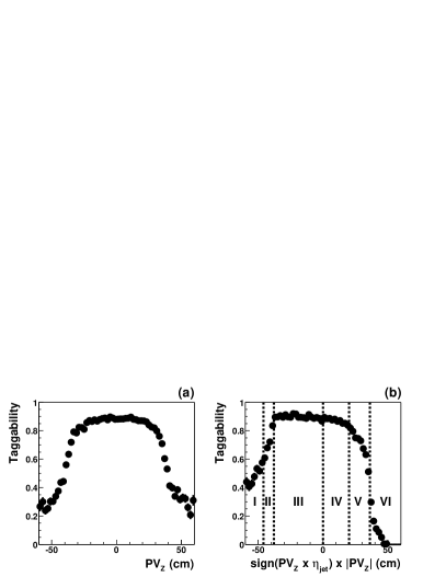
Figure 2: Taggability vs. (a) $PV_{z}$ and (b) ${\rm sign}(PV_{z}\times\eta)\times|PV_{z}|$ as measured in data. The dashed lines correspond to the boundaries between regions defined in the text.

A two-dimensional parameterization of the taggability vs. jet $p_{T}$ and $|\eta|$ is derived by assuming that the dependence is factorizable, so that $\varepsilon(p_{T},\eta)=C\varepsilon(p_{T})\varepsilon(\eta)$. The normalization factor $C$ is such that the total number of observed taggable jets equals the number of predicted taggable jets, calculated as the sum over all reconstructed jets weighted by their corresponding $\varepsilon(p_{T},\eta)$. Figure 3 shows $\varepsilon(p_{T})$ and $\varepsilon(\eta)$ for the six regions defined above.

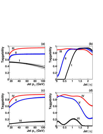
Figure 3: Taggability vs. jet $p_{T}$ and $|\eta|$ for $PV_{z}\times\eta<0$ [(a) and (b) respectively] and $PV_{z}\times\eta>0$ [(c) and (d) respectively]. The central value is shown with a solid line, and the $\pm 1\sigma$ statistical uncertainty is shown as dotted lines. The labels I$-$VI correspond to the regions of ${\rm sign}(PV_{z}\times\eta)\times|PV_{z}|$ defined in Fig. 2.

The assumption that the taggability can be factorized in terms of jet $p_{T}$ and $\eta$ is verified through a validation test closure that compares the numbers of predicted and observed taggable jets as functions of jet $p_{T}$, $\eta$, $PV_{z}$, and number of jets. For this study, the combined $l+$jets taggability parameterization is applied separately to the $e$+jets and $\mu$+jets preselected samples as a weight for each jet. Statistical uncertainties of the fits used to derive the parameterizations are assigned as errors to the taggability. Good agreement between predicted and observed distributions is observed for all variables.

VII.1.2 Jet Flavor Dependence of Taggability

The taggability measured in data is dominated by the predominant light quark jet contribution to the low jet multiplicity bins. The ratios of $b$ to light and $c$ to light taggabilities as functions of jet $p_{T}$ and $\eta$ are measured in a QCD multijet MC sample and shown in Fig. 4. The largest difference in taggability, approximately 5%, is observed between $b$ and light quark jets in the low $p_{T}$ region, corresponding to jets with low track multiplicity. The fits to the ratios are used as flavor dependent correction factors to the taggability.

The systematic uncertainty on the flavor dependence of the taggability is estimated by substituting the parameterization for $b$ and $c$ quark jets with the one determined from $Wb\bar{b}$ and $Wc\bar{c}$ MC, respectively. The default $b$-flavor ($c$-flavor) parameterization is retained for the central value and the observed difference between that one and the $Wb\bar{b}$ ($Wc\bar{c}$) parameterization is taken as the systematic uncertainty.

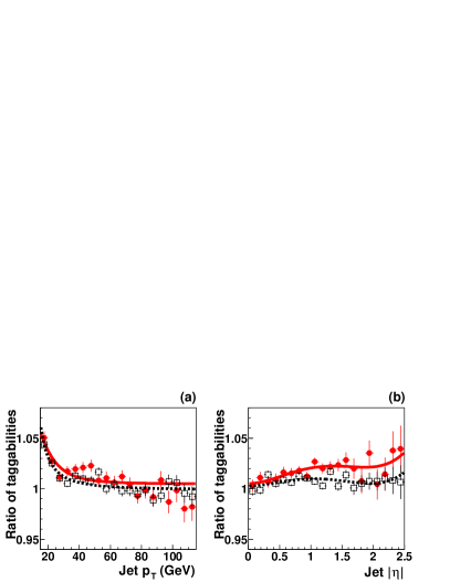
Figure 4: Ratio of the $b$ to light (full circles) and $c$ to light (open squares) quark jet taggability, measured in a QCD MC sample as functions of (a) jet $p_{T}$ and (b) jet $|\eta|$. The resulting fits used in the analysis are also shown.

In comparison with light quark jets, hadronic tau lepton decays have a lower average track multiplicity and are therefore expected to have lower taggability. Figure 5 shows the ratio of $\tau$ to light quark jet taggability as functions of jet $p_{T}$ and $\eta$ as measured in $Z/\gamma^{*}\rightarrow\tau\tau$ and $Z/\gamma^{*}\rightarrow q\bar{q}$ MC samples. The fit to the ratio is used as a flavor dependent correction factor to the taggability of hadronic tau decays in the estimation of the $Z/\gamma^{*}\rightarrow\tau\tau$ background.

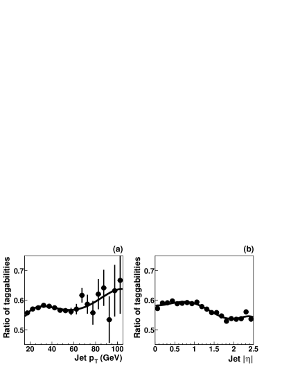
Figure 5: Ratio of the hadronic $\tau$ to light quark jet taggability, measured in $Z/\gamma^{*}\rightarrow\tau\tau$ and $Z/\gamma^{*}\rightarrow q\bar{q}$ MC samples as functions of jet $p_{T}$ (a) and jet $|\eta|$ (b). The resulting fits used in the analysis are also shown.

VII.2 Tagging Efficiency

The $b$ and $c$ quark jet tagging efficiencies are measured in a $t\overline{t}$ MC sample and calibrated to data using a data-to-MC scale factor derived from a sample dominated by semileptonic $b\bar{b}$ decays. The efficiency of tagging a light quark jet is measured in a data sample dominated by light quark jets and corrected for contamination of heavy flavor jets and long-lived particles ($K_{S}^{0}$, $\Lambda^{0}$). The procedures followed to determine each of the tagging efficiencies and their corresponding uncertainties are summarized below.

VII.2.1 Semileptonic $b$ Tagging Efficiency

The tagging efficiency for $b$ quarks that decay semileptonically to muons is referred to as the semileptonic $b$ tagging efficiency. It is measured in data using a system of eight equations (System8 Method) constructed from the total number of events in two samples with different $b$ jet content, before and after tagging with two $b$ tagging algorithms. The two data samples used are the muon-in-jet ($n$) and the muon-in-jet-away-jet-tagged sample ($p$) (see Sec. IV.7 for the definition of these samples). The two $b$ tagging algorithms are SVT and the soft lepton tagger (SLT). The SLT algorithm requires the presence of a muon with $\Delta R(\mu,\text{jet})<0.5$ and $p_{T}^{\text{rel}}>0.7$ GeV within the jet, where $p_{T}^{\text{rel}}$ refers to the muon momentum transverse to the momentum of the jet-muon system. The jets are divided in two categories: $b$ jets, and $c+$light ($cl$) jets, and the following system of eight equations is written:

$$n = n_{b}+n_{cl}$$

$$p = p_{b}+p_{cl}$$

$$n^{\text{SVT}} = \varepsilon_{b}^{\text{SVT}}n_{b}+\varepsilon_{cl}^{\text{SVT}}n_{cl}$$

$$p^{\text{SVT}} = \beta\;\varepsilon_{b}^{\text{SVT}}p_{b}+\alpha\;\varepsilon_{cl}^{\text{SVT}}p_{cl}$$

$$n^{\text{SLT}} = \varepsilon_{b}^{\text{SLT}}n_{b}+\varepsilon_{cl}^{\text{SLT}}n_{cl}$$

$$p^{\text{SLT}} = \varepsilon_{b}^{\text{SLT}}p_{b}+\varepsilon_{cl}^{\text{SLT}}p_{cl}$$

$$n^{\text{SVT},\text{SLT}} = \kappa_{b}\;\varepsilon_{b}^{\text{SVT}}\varepsilon_{b}^{\text{SLT}}n_{b}+\kappa_{cl}\;\varepsilon_{cl}^{\text{SVT}}\varepsilon_{cl}^{\text{SLT}}n_{cl}$$

$$p^{\text{SVT},\text{SLT}} = \kappa_{b}\;\beta\;\varepsilon_{b}^{\text{SVT}}\varepsilon_{b}^{\text{SLT}}p_{b}+\kappa_{cl}\;\alpha\;\varepsilon_{cl}^{\text{SVT}}\varepsilon_{cl}^{\text{SLT}}p_{cl}\;.$$

The terms on the left hand side represent the total number of jets in each sample before tagging ($n$, $p$) and after tagging with the SVT algorithm ($n^{\text{SVT}},p^{\text{SVT}}$), the SLT algorithm ($n^{\text{SLT}},p^{\text{SLT}}$), and both ($n^{\text{SVT,SLT}},p^{\text{SVT,SLT}}$). The eight unknowns on the right hand side of the equations consist of the number of $b$ and $c+$light jets in the two samples ($n_{b}$, $n_{cl}$, $p_{b}$, $p_{cl}$), and the tagging efficiencies for $b$ and $c+$light jets for the two tagging algorithms ($\varepsilon_{b}^{\text{SVT}},\varepsilon_{b}^{\text{SLT}},\varepsilon_{cl}^{\text{SVT}},\varepsilon_{cl}^{\text{SLT}}$). The method assumes that the efficiency for tagging a jet with both the SVT and the SLT algorithm can be calculated as the product of the individual tagging efficiencies. Four additional parameters are needed to solve the system of equations: $\kappa_{b}$, $\kappa_{cl}$, $\alpha$, and $\beta$. The first two parameters represent the correlation between the SVT and the SLT tagger for $b$ jets ($\kappa_{b}$) and $c+$light jets ($\kappa_{cl}$), respectively. They are defined as

$$\kappa_{b}=\frac{\varepsilon_{b}^{\text{SVT},\text{SLT}}}{\varepsilon_{b}^{\text{SVT}}\varepsilon_{b}^{\text{SLT}}}\,,$$

and

$$\kappa_{cl}=\frac{\varepsilon_{cl}^{\text{SVT},\text{SLT}}}{\varepsilon_{cl}^{\text{SVT}}\varepsilon_{cl}^{\text{SLT}}}\,.$$

$\beta$ and $\alpha$ represent the ratio of the SVT tagging efficiencies for $b$ and $c+$light jets, respectively, corresponding to the two data samples used to solve System8. They are defined as

$$\beta=\frac{\varepsilon_{b}^{\text{SVT}}\text{from muon-in-jet-away-jet-tagged sample}}{\varepsilon_{b}^{\text{SVT}}\text{from muon-in-jet sample}}\,,$$

and

$$\alpha=\frac{\varepsilon_{cl}^{\text{SVT}}\text{from muon-in-jet-away-jet-tagged sample}}{\varepsilon_{cl}^{\text{SVT}}\text{from muon-in-jet sample}}\,.$$

$\kappa_{b}$, $\kappa_{cl}$, and $\beta$ are measured in a MC sample mixture of $Z/\gamma^{*}\rightarrow b\bar{b}\rightarrow\mu$, $Z/\gamma^{*}\rightarrow c\bar{c}$, $Z/\gamma^{*}\rightarrow q\bar{q}$, QCD multijet, and $t\overline{t}$, giving $\kappa_{b}=0.978\pm 0.002$, $\kappa_{cl}=0.826\pm 0.014$, and $\beta=0.999\pm 0.006$. $\alpha$ is arbitrarily chosen to be $1.0\pm 0.8$.

The system of equations is solved for each $p_{T}$ and $\eta$ bin separately. The resulting semileptonic $b$ tagging efficiency for the SVT algorithm is shown in Fig. 6.

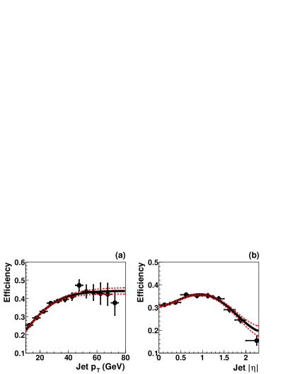
Figure 6: Semileptonic $b$ tagging efficiency vs. jet $p_{T}$ (a) and jet $|\eta|$ (b) measured in data with the System8 method. The resulting fit is shown as a solid line, and the $\pm 1\sigma$ statistical uncertainty is shown as dotted lines.

The statistical uncertainty is given by the error on the fit to the parameterization as functions of jet $p_{T}$ and $|\eta|$. The systematic uncertainties are obtained from the change in the semileptonic $b$ tagging efficiency resulting from the variation on the correlation parameters $\alpha$, $\beta$, $\kappa_{b}$ and $\kappa_{cl}$. $\beta$ and $\kappa_{cl}$ are varied within the uncertainties obtained when the distributions of $\beta$ and $\kappa_{cl}$ as functions of jet $p_{T}$ are fitted to constants. The variation of $\kappa_{b}$ is determined from the difference between the value of $\kappa_{b}$ obtained in the MC sample described above and those obtained from $Z/\gamma^{*}\rightarrow b\bar{b}$ and $t\bar{t}$ MC samples. Another source of systematic uncertainty comes from the choice of the $p_{T}^{\text{rel}}$ cut used in the SLT tagger.

VII.2.2 Measurement of the Inclusive Tagging Efficiencies

The inclusive $b$ and $c$ tagging efficiencies are measured in a MC $t\overline{t}$ sample and calibrated by a data-to-MC scale factor given by the ratio of the semileptonic $b$ tagging efficiency as measured in data to the one measured in a $b\bar{b}$ MC sample. The $b\bar{b}$ MC is chosen to determine the scale factor because it is expected to best simulate the data samples used in the System8 fit. With this procedure, the topological dependence of the tagging efficiencies is taken from the $t\overline{t}$ sample, and the overall efficiency normalization is calibrated to data. Figure 7 shows the semileptonic $b$ tagging efficiency as measured in the $b\bar{b}$ MC sample. Figure 8 shows the inclusive $b$ and $c$ tagging efficiencies that are used in the analysis.

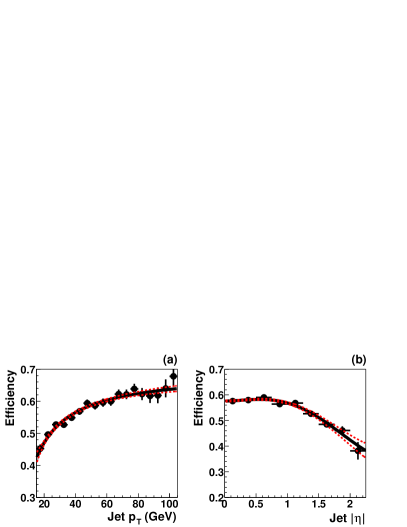
Figure 7: Semileptonic $b$ tagging efficiency vs. (a) jet $p_{T}$ and (b) jet $|\eta|$ measured in a $b\bar{b}$ MC sample. The resulting fit is shown as a solid line, and the $\pm 1\sigma$ statistical uncertainty is shown as dotted lines.

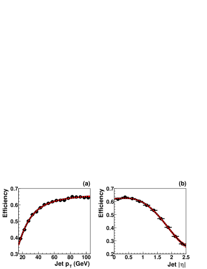
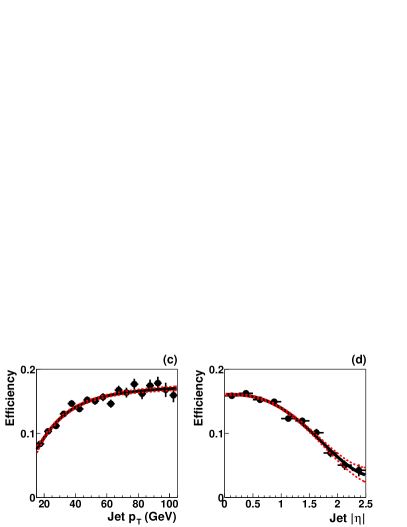
Figure 8: Inclusive $b$ tagging efficiency vs. (a) jet $p_{T}$ and (b) jet $|\eta|$ and inclusive $c$ tagging efficiency vs. (c) jet $p_{T}$ and (d) jet $|\eta|$. The resulting fit is shown as a solid line, and the $\pm 1\sigma$ statistical uncertainty is shown as dotted lines.

The systematic uncertainty on the semileptonic $b$ tagging efficiency from MC is taken as the difference between the 2D parameterization obtained from $b\bar{b}$ MC and the one derived from a $t\overline{t}$ MC sample. For the inclusive $b$ and $c$ tagging efficiencies, the systematic uncertainty is taken as the difference between the 2D parameterizations obtained from $t\overline{t}$ MC samples with two choices of $b$ fragmentation models bFF . In both cases, the systematic uncertainties in each $p_{T}$ and $\eta$ bin are added in quadrature to the corresponding statistical uncertainty arising from the fit giving the default parameterization.

A closure test closure of the parameterized MC tagging efficiency is performed in each case on the MC sample used to derive the default parameterization. In addition, a validation is performed on a matched $W$+jets sample (Appendix A) that has passed the preselection cuts. In both cases, the predicted tags are compared with the observation as functions of jet $p_{T}$, $\eta$, and jet multiplicity. Good agreement between prediction and observation is observed in all cases.

The hadronic $\tau$ tagging efficiency is measured in a $Z/\gamma^{*}\rightarrow\tau\tau$ MC sample and assigned a 50% systematic uncertainty. In this analysis, the hadronic $\tau$ tagging efficiency is used only in the estimation of the $Z/\gamma^{*}\rightarrow\tau\tau$ background.

VII.3 Measurement of the Mistag Rate

Mistags are defined as light flavor jets that have been tagged by the SVT algorithm from random overlap of tracks that are displaced from the PV due to tracking errors or resolution effects. Since the SVT algorithm is symmetric in its treatment of both the impact parameter and the decay length significance $L_{xy}/\sigma(L_{xy})$, the mistags are expected to occur at the same rate for positive tags ($L_{xy}/\sigma(L_{xy})>7.0$) and for negative tags ($L_{xy}/\sigma(L_{xy})<-7.0$). The negative tagging rate measured in a sample dominated by light jets can therefore be used to extract the mistag rate after correcting for the contamination of heavy flavor ($hf$) jets in the negative tags, and the presence of long lived particles ($ll$) in the positive tags.

For this analysis, the negative tagging efficiency is measured in the EMqcd data sample, which is dominated by QCD multijet production, and parameterized as functions of jet $p_{T}$ and $\eta$, as shown in Fig. 9. A closure test of the parameterization is performed by comparing the predicted rates of negative tags to the observed one in the same sample used to derive the parameterizations. Good agreement is observed in all distributions for jet $p_{T}$, $|\eta|$, and jet multiplicity.

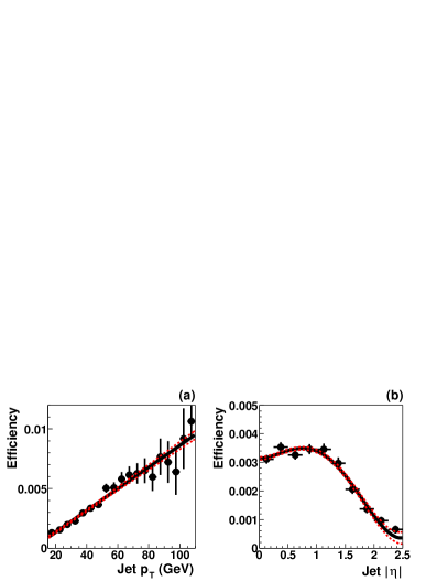
Figure 9: Negative tagging efficiency vs. (a) jet $p_{T}$ and (b) jet $|\eta|$. The resulting fit is shown as a solid line, and the $\pm 1\sigma$ statistical uncertainty is shown as dotted lines.

The parameterized negative tag rate is also applied to all taggable jets in the preselected samples, and the prediction is compared to the actual number of observed negative tags. The results are summarized in Table 5 and show good agreement between prediction and observation.

	1 jet	2 jet	3 jet	$\geq$ 4 jet
$e$+jets channel
$N^{\text{pred}}$	24.6$\pm$5.0	13.4$\pm$3.7	3.89$\pm$1.97	1.54$\pm$1.24
$N^{\text{obs}}$	22	16	5	4
$\mu$+jets channel
$N^{\text{pred}}$	34.3$\pm$5.9	17.5$\pm$4.2	4.55$\pm$2.13	1.44$\pm$1.20
$N^{\text{obs}}$	32	13	6	1
$l$+jets channel
$N^{\text{pred}}$	58.9$\pm$7.7	30.9$\pm$5.6	8.44$\pm$2.90	2.98$\pm$1.73
$N^{\text{obs}}$	54	29	11	5

Table 5: Numbers of observed and predicted negative tags in the preselected signal samples.

To be able to use this measurement to estimate mistags from light quark jets, a correction is needed since the data sample is expected to contain a small contribution from $b$ and $c$ jets ($\approx 2\%$ and $\approx 4\%$, respectively, as predicted by pythia) that have a higher negative tagging efficiency than light quark jets. A correction factor $SF_{hf}$ is derived from pythia QCD multijet MC as the ratio between the negative tagging rate for light quark jets and the one obtained for an inclusive jet sample

$$SF_{hf}(p_{T},\eta)=\frac{\varepsilon^{\text{light}}_{-}(p_{T},\eta)}{\varepsilon^{\text{inclusive}}_{-}(p_{T},\eta)}\,.$$

In addition, the long-lived particles present in the EMqcd sample lead to a larger positive than negative tagging efficiency. A correction factor $SF_{ll}$ is derived from pythia QCD multijet MC as the ratio between the positive and the negative tagging rates for light jets

$$SF_{ll}(p_{T},\eta)=\frac{\varepsilon^{\text{light}}_{+}(p_{T},\eta)}{\varepsilon^{\text{light}}_{-}(p_{T},\eta)}.$$

Both scale factors are shown in Fig. 10. Finally, the mistag rate is given by

$$\varepsilon^{\text{light}}_{+}(p_{T},\eta)=\varepsilon^{\text{data}}_{-}(p_{T},\eta)SF_{hf}(p_{T},\eta)SF_{ll}(p_{T},\eta)\,.$$

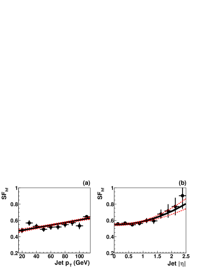
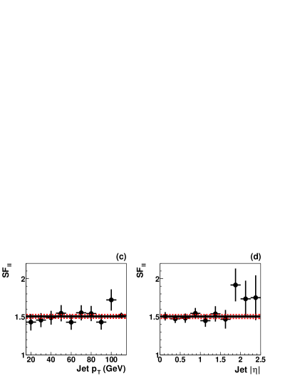
Figure 10: Correction factors for the contribution of heavy flavor in the negative tag rate ($SF_{hf}$) as functions of (a) jet $p_{T}$ and (b) jet $|\eta|$ and contribution to the mistag rate from long lived particles ($SF_{ll}$) as functions of (c) jet $p_{T}$ and (d) jet $|\eta|$. The resulting fits are shown as solid lines, and the $\pm 1\sigma$ statistical uncertainties are shown as dotted lines.

The systematic uncertainty on the mistag rate is determined by coherently varying by 20% the $b$ and $c$ fractions in the pythia QCD multijet MC sample used to measure $SF_{hf}$ and $SF_{ll}$. The resulting systematic uncertainty in each $p_{T}$ and $\eta$ bin is added in quadrature to the corresponding statistical uncertainty arising from the fit giving the default parameterization for $\varepsilon^{\text{data}}_{-}$, $SF_{hf}$, and $SF_{ll}$.

VII.4 Event Tagging Probability

The probability for a jet of a given flavor $\alpha$ ($b$, $c$, or light quark jet) to be tagged is obtained as the product of the taggability and the calibrated tagging efficiency

$${\mathcal{P}}_{\alpha}(p_{T},\eta)=P^{\text{taggab}}_{\alpha}(p_{T},\eta)\varepsilon_{\alpha}(p_{T},\eta).$$

The probability for a given MC event to contain at least one SVT-tagged jet is given by the complement of the probability that none of the jets is tagged:

$$P^{\text{tag}}_{\text{event}}(\geq 1\;\mathrm{tag})=1-P^{\text{tag}}_{\text{event}}(0\;\mathrm{tag})\,,$$

with

$$P^{\text{tag}}_{\text{event}}(0\;\mathrm{tag})=\prod_{j=1}^{N_{\text{jets}}}[1-{\mathcal{P}}_{\alpha_{j}}(p_{T_{j}},\eta_{j})]\,.$$

The probabilities for a given MC event to have exactly one or to have two or more SVT tagged jets are given by

$$P^{\text{tag}}_{\text{event}}(1\;\mathrm{tag})=\sum_{j=1}^{N_{\text{jets}}}{{\mathcal{P}}_{\alpha_{j}}(p_{T_{j}},\eta_{j})}\prod_{i\neq j}[1-{\mathcal{P}}_{\alpha_{i}}(p_{T_{i}},\eta_{i})]\,,$$

and

$$P^{\text{tag}}_{\text{event}}(\geq 2\;\mathrm{tag})=P^{\text{tag}}_{\text{event}}(\geq 1\;\mathrm{tag})-P^{\text{tag}}_{\text{event}}(1\;\mathrm{tag})\,,$$

respectively. $P^{\text{tag}}_{\text{event}}(1\;\mathrm{tag})$ and $P^{\text{tag}}_{\text{event}}(\geq 2\;\mathrm{tag})$ are referred to as single and double tagging probabilities, respectively.

The average event tagging probability for a certain process $P^{\text{tag}}_{\text{process}}$ is calculated by averaging the per-event SVT tagging probability over a sample of events for the process under consideration. The probability for an event to satisfy the trigger conditions is included in the calculation, as the trigger can distort the jet $p_{T}$ and $\eta$ spectra, particularly for the low jet multiplicity bins.

The trigger-corrected average event tagging probability is measured for MC $t\overline{t}$ events that pass the preselection and originated from the processes $t\bar{t}\rightarrow l$+jets and $t\bar{t}\rightarrow ll$; the results are summarized in Table 6.

	$e$+jets								$\mu$+jets
	$1~{}\mathrm{jet}$		$2~{}\mathrm{jets}$		$3~{}\mathrm{jets}$		$\geq 4~{}\mathrm{jets}$		$1~{}\mathrm{jet}$		$2~{}\mathrm{jets}$		$3~{}\mathrm{jets}$		$\geq 4~{}\mathrm{jets}$
$t\overline{t}$ single tag probabilities (%)
$t\bar{t}\rightarrow l$+jets	26.6$\pm$	0.7	38.7$\pm$	0.2	43.3$\pm$	0.1	44.7$\pm$	0.1	26.2$\pm$	0.9	37.8$\pm$	0.2	42.7$\pm$	0.1	44.1$\pm$	0.1
$t\bar{t}\rightarrow ll$	38.8$\pm$	0.2	44.7$\pm$	0.1	44.9$\pm$	0.2	44.6$\pm$	0.5	38.4$\pm$	0.3	44.0$\pm$	0.1	44.5$\pm$	0.2	44.1$\pm$	0.5
$t\overline{t}$ double tag probabilities (%)
$t\bar{t}\rightarrow l$+jets			4.93$\pm$	0.10	11.5$\pm$	0.1	15.4$\pm$	0.1			5.06$\pm$	0.11	11.5$\pm$	0.1	15.2$\pm$	0.1
$t\bar{t}\rightarrow ll$			12.4$\pm$	0.1	13.6$\pm$	0.1	14.1$\pm$	0.4			12.1$\pm$	0.1	13.6$\pm$	0.1	13.5$\pm$	0.4

Table 6: Summary of the average event tagging probabilities (%) for $t\overline{t}$ events that pass the preselection and originate from the processes $t\bar{t}\rightarrow l$+jets and $t\bar{t}\rightarrow ll$. Statistical uncertainties only are quoted.

VIII Composition of the Tagged Sample

The main background to the tagged $l$+jets sample is heavy flavor production in association with a $W$ boson. Additional contributions arise from direct QCD heavy flavor production, other low rate electroweak processes (single top, diboson, and $Z/\gamma^{*}\to\tau\tau$ production), as well as mistags of light quark jets. The methods used to estimate the contribution from these background processes are described below.

VIII.1 Evaluation of the $W$+jets Background

Available MC generators are able to perform matrix element calculations for $W$+jets events with high jet multiplicities only at leading order. As a result, the overall normalization of the calculations suffers from large theoretical uncertainties, although the relative contributions of the different processes are well described. In this analysis, the overall normalization of the $W$+jets contribution is obtained directly from collider data, and only the relative contributions of different processes are taken from MC. The contribution of $W$+jets events to the tagged sample is then estimated by multiplying the number of $W$+jets events of each type in the preselected sample by the SVT efficiency corresponding to the type of process under consideration, as described below.

The overall normalization of the $W$-like background in the preselected sample before tagging ($N^{\text{sig}}_{t}$) is obtained directly from collider data as described in Sec. VI. $N^{\text{sig}}_{t}$ consists mostly of $W$+jets background events, with contributions from $t\overline{t}$ and other low rate electroweak processes. Thus, the number of $W$+jets events in the preselected sample can be calculated as

$$N^{\text{presel}}_{W+\text{jets}} = N^{\text{sig}}_{t}-N_{t\bar{t}\rightarrow l+\text{jets}}^{\text{presel}}-N_{t\bar{t}\rightarrow ll}^{\text{presel}}$$

$$- \sum_{\text{bkg}\;i}{N}_{\text{bkg}\;i}^{\text{presel}}\,,$$

where $i$ loops over the electroweak backgrounds. It is important to note that $N_{t\bar{t}\rightarrow l+\text{jets}}^{\text{presel}}$ and $N_{t\bar{t}\rightarrow ll}^{\text{presel}}$ are allowed to float during the extraction of the $t\overline{t}$ cross section, adjusting the $W$+jets contribution accordingly.

The predicted number of $W$+jets events in the tagged sample is obtained by multiplying the estimated number of preselected $W$+jets events by the corresponding average event tagging probability $P^{\text{tag}}_{W+\text{jets}}$:

$$N^{\text{tag}}_{W+\text{jets}}=N^{\text{presel}}_{W+\text{jets}}P^{\text{tag}}_{W+\text{jets}}\,.$$

$P^{\text{tag}}_{W+\text{jets}}$ is obtained by adding the tagging probabilities for the different flavor configurations considered, weighted by their fractions within a given jet multiplicity bin

$$P^{\text{tag}}_{W+\text{jets}}=\sum_{\Phi_{n}}F_{\Phi_{n}}\,P^{\text{tag}}_{\Phi_{n}}.$$

$F_{\Phi_{n}}$ gives the fraction of events that pass the preselection for each flavor configuration $\Phi$ per jet multiplicity bin $n$. It is determined by:

$$F_{\Phi,n}=\frac{\sigma^{\mathrm{eff}}_{\Phi,n}}{\sum_{\Phi}\sigma^{\mathrm{eff}}_{\Phi,n}}\,,$$

where $\sigma^{\mathrm{eff}}_{\Phi,n}\equiv\sigma_{\Phi,n}\cdot\varepsilon^{\text{presel},\text{match}}_{\Phi,n}$ is the effective cross section, obtained by multiplying the theoretical cross section $\sigma_{\Phi,n}$ from alpgen by the preselection and matching efficiency $\varepsilon^{\text{presel},\text{match}}_{\Phi,n}$ for each flavor configuration and jet multiplicity. The flavor configurations considered in the analysis were identified according to the ad hoc matching prescription discussed in Appendix A and are summarized in Table 7. $P^{\text{tag}}_{\Phi_{n}}$ is the corresponding average event tagging probability, as defined in Sec. VII.4. The resulting event tagging probabilities for each $W$+jets flavor subprocess are summarized in Table 8.

Contribution	$W$+1 jet		$W$+2 jets		$W$+3 jets		$W$+$\geq$4 jets
$Wb\bar{b}$			$1.23$$\pm$	$0.08$	$2.05$$\pm$	$0.21$	$2.84$$\pm$	$0.16$
$Wc\bar{c}$			$1.69$$\pm$	$0.12$	$2.94$$\pm$	$0.37$	$4.44$$\pm$	$0.29$
$W(b\bar{b})$	$0.86$$\pm$	$0.03$	$1.46$$\pm$	$0.09$	$2.03$$\pm$	$0.15$	$2.99$$\pm$	$0.24$
$W(c\bar{c})$	$1.23$$\pm$	$0.05$	$2.26$$\pm$	$0.15$	$3.08$$\pm$	$0.24$	$5.06$$\pm$	$0.54$
$Wc$	$4.41$$\pm$	$0.18$	$6.25$$\pm$	$0.43$	$4.93$$\pm$	$0.48$	$4.30$$\pm$	$0.23$
$W$+light	$93.5$$\pm$	$0.2$	$87.1$$\pm$	$0.7$	$85.0$$\pm$	$1.1$	$80.4$$\pm$	$0.7$

Table 7: Fractions (%) of different $W$+jets flavor subprocesses contributing to each jet multiplicity bin when ad hoc matching and preselection are required. Statistical uncertainties only are quoted.

The choice of cone size used for the ad hoc matching procedure contributes to the systematic uncertainty. To estimate this effect, the cone size is varied from the default value of $\Delta R=0.5$ to $\Delta R=0.7$, and the difference, centered on the default value, is assigned as the systematic uncertainty on the fractions. This results in a relative uncertainty of 2% for the $Wc$ fractions and 5% for the $Wb\bar{b}$, $W(b\bar{b})$, $Wc\bar{c}$, and $W(c\bar{c})$ fractions, in all jet multiplicities (refer to Appendix A for a definition of these samples). In addition, the $W$+jets fractions are also derived from limited-statistics MC samples where matrix element partons are matched to particle jets following the MLM matching scheme Mangano . The difference between the fractions obtained from these samples and the ones derived from samples matched with the ad hoc method is less than 20% for the region of interest (events with three or more jets), and does not depend on the choice of matching parameters. An additional 20% systematic uncertainty is assigned to the $W$+jets fractions based on this study.

The fractions calculated with both matching procedures are obtained from MC samples based on LO calculations. Several studies mcfm ; Campbell of $W$+2 jets processes have established that the ratio of $Wb\bar{b}$ to $Wjj$ cross sections at NLO is higher by a factor $K=1.05\pm 0.07$ compared to the LO prediction. The systematic uncertainty on the $K$-factor arises from the residual dependence on the factorization scale and from the uncertainty on the PDFs, which is obtained using the 20 eigenvector pairs for the CTEQ6M PDFs CTEQ6 . This $K$-factor is applied to correct the ad hoc fractions of $Wb\bar{b}$, $W(b\bar{b})$, $Wc\bar{c}$, and $W(c\bar{c})$, while for the $Wc$ fraction, the LO prediction is used. The fraction of $W+$light jets is adjusted to ensure that the sum of all fractions equals 1.

Additional systematic uncertainties associated with the $W$ boson modeling arise from the choice of parton distribution functions, factorization scale, and heavy quark mass. The systematic uncertainty arising from each of these factors on the $W$+jets fractions is calculated from the relative change in the alpgen cross section, properly taking correlations into account. The PDF uncertainty is calculated using the 20 eigenvector pairs from CTEQ6M; the factorization scale uncertainty is calculated by varying the scale to two times and one-half of the default value; the heavy quark mass uncertainty is calculated by varying by $\pm 0.3$ GeV pdg the heavy quark masses with respect to their default values ($m_{b}=4.75$ GeV and $m_{c}=1.55$ GeV).

An alternative method of obtaining the event tagging probability for $W$+light jets is to apply the light tagging efficiency parameterization directly to the preselected signal sample. Under the assumption that the preselected sample is dominated by $W$+light jets events, this method has the advantage of taking the kinematic information directly from the data. The event tagging probabilities obtained with this alternative method are also shown in Table 8 and are in good agreement with those obtained from MC.

The expected number of $W$+jets events for each flavor subprocess as a function of jet multiplicity are summarized in Tables 9 and 10 for single and double tagged events, respectively.

	$e$+jets								$\mu$+jets
	$W$+1 jet		$W$+2 jets		$W$+3 jets		$W$+$\geq$4 jets		$W$+1 jet		$W$+2 jets		$W$+3 jets		$W$+$\geq$4 jets
Single tag probabilities (%)
$W$+light	0.40$\pm$	0.01	0.64$\pm$	0.02	0.90$\pm$	0.05	1.37$\pm$	0.14	0.39$\pm$	0.01	0.62$\pm$	0.02	0.89$\pm$	0.05	1.23$\pm$	0.14
$W$+light	0.39$\pm$	0.01	0.62$\pm$	0.04	0.90$\pm$	0.02	1.32$\pm$	0.06	0.41$\pm$	0.01	0.74$\pm$	0.04	0.92$\pm$	0.03	1.23$\pm$	0.05
$W(c\bar{c})$	9.3$\pm$	0.1	8.6$\pm$	0.3	8.9$\pm$	0.2	9.2$\pm$	0.9	9.4$\pm$	0.1	9.2$\pm$	0.2	8.6$\pm$	0.1	10.2$\pm$	0.7
$W(b\bar{b})$	38.4$\pm$	0.4	35.4$\pm$	0.6	34.5$\pm$	0.4	34.9$\pm$	1.9	38.5$\pm$	0.4	36.3$\pm$	0.6	33.7$\pm$	0.4	35.8$\pm$	1.5
$Wc$	9.6$\pm$	0.1	9.6$\pm$	0.2	9.7$\pm$	0.3	10.2$\pm$	0.3	9.6$\pm$	0.1	9.4$\pm$	0.2	9.4$\pm$	0.3	9.7$\pm$	0.3
$Wc\bar{c}$			15.6$\pm$	0.4	14.8$\pm$	1.1	16.4$\pm$	0.6			16.0$\pm$	0.4	16.2$\pm$	0.7	16.3$\pm$	0.6
$Wb\bar{b}$			43.8$\pm$	0.7	45.6$\pm$	0.9	44.5$\pm$	0.9			44.0$\pm$	0.8	44.0$\pm$	1.0	44.0$\pm$	0.8
$W$+jets	1.23$\pm$	0.01	2.66$\pm$	0.04	3.59$\pm$	0.05	5.03$\pm$	0.07	1.25$\pm$	0.01	2.78$\pm$	0.04	3.57$\pm$	0.04	4.97$\pm$	0.08
Double tag probabilities (%)
$W$+light			$<0.01$		$<0.01$		$<0.01$				$<0.01$		$<0.01$		$<0.01$
$W(c\bar{c})$			0.03$\pm$	0.01	0.09$\pm$	0.01	0.14$\pm$	0.05			0.04$\pm$	0.01	0.08$\pm$	0.01	0.14$\pm$	0.04
$W(b\bar{b})$			0.49$\pm$	0.09	0.97$\pm$	0.09	0.52$\pm$	0.11			0.96$\pm$	0.15	0.77$\pm$	0.07	1.35$\pm$	0.39
$Wc$			0.023$\pm$	0.002	0.052$\pm$	0.004	0.082$\pm$	0.004			0.030$\pm$	0.002	0.051$\pm$	0.004	0.074$\pm$	0.004
$Wc\bar{c}$			0.76$\pm$	0.04	0.75$\pm$	0.10	0.97$\pm$	0.08			0.80$\pm$	0.04	0.94$\pm$	0.10	1.05$\pm$	0.09
$Wb\bar{b}$			12.2$\pm$	0.5	13.1$\pm$	0.8	14.1$\pm$	0.6			13.0$\pm$	0.4	12.5$\pm$	0.7	12.8$\pm$	0.5
$W$+jets			0.17$\pm$	0.01	0.32$\pm$	0.02	0.48$\pm$	0.02			0.19$\pm$	0.01	0.31$\pm$	0.01	0.47$\pm$	0.02

Table 8: Tagging probabilities (%) for preselected $W$+jets events for single tags (top rows) and double tags (bottom rows). The uppermost row labeled $W$+light corresponds to the efficiencies obtained from applying the light tagging efficiency parameterization to the preselected signal sample. The rows labeled $W$+jets summarize the average event tagging probabilities for $W$ boson events. These values are not used in the analysis and are included for informational purposes only. In all cases, statistical uncertainties only are quoted.

VIII.2 Evaluation of the QCD Multijet Background

The QCD multijet background is evaluated by applying the matrix method directly to the tagged samples. Equation VI, originally defined for the preselected data in Sec. VI, can be re-written for the single and double tagged samples and directly solved to obtain the number of QCD multijet events in the tagged samples. The rate at which a loose lepton in QCD multijet events appears to be tight is remeasured for the tagged samples and found to agree with the one used for the preselected samples.

As a cross check, the QCD multijet background in the single tagged $e$+jets sample is obtained by multiplying the number of QCD multijet events in the preselected sample ($N_{t}^{\text{QCD}}$) by the corresponding average event tagging probability $P^{\text{tag}}_{\text{QCD}}$, defined as the fraction of tagged events in the loose-minus-tight $e$+jets sample. The estimated number of tagged events is then given by

$$N^{\text{tag}}_{\text{QCD}}=N_{t}^{\text{QCD}}P^{\text{tag}}_{\text{QCD}}\,.$$

Good agreement is observed between the matrix method and the cross check.

The cross check assumes that the heavy flavor composition in the loose-minus-tight data sample, where the average event tagging probability is derived, is identical to the heavy flavor composition of the QCD multijet background in the preselected sample. In the $e$+jets channel this assumption applies, since the instrumental background mainly originates from electromagnetically fluctuating jets misreconstructed as electrons. In the $\mu$+jets channel however, the instrumental background originates mainly from semileptonically decaying $b$ quarks to muons; the heavy flavor fraction is therefore enriched when the isolation criteria is inverted, leading to a higher event tagging probability. As the cross check cannot be applied to the $\mu$+jets channel, results from the matrix method are used to extract the cross section in both the $e$+jets and the $\mu$+jets channel.

Tables 9 and 10 summarize the expected number of QCD multijet events as a function of jet multiplicity for single and double tag events, respectively.

VIII.3 Physics Backgrounds

Additional low rate electroweak processes that contribute to the tagged sample are diboson production ($WW\rightarrow l+\text{jets}$, $WZ\rightarrow l+\text{jets}$, $WZ\rightarrow jjl\bar{l}$, $ZZ\rightarrow l\bar{l}jj$), single top quark $s$- and $t$-channel production, and $Z/\gamma^{*}\rightarrow\tau\tau\rightarrow l+\text{jets}$, where one $\tau$ decays leptonically and the second one hadronically. The $Z$+jets background where one of the two leptons is not reconstructed is found to be negligible.

For a given process $i$, the number of events before tagging is determined as

$${N}_{\text{bkg}\;i}^{\text{presel}} = \sigma_{i}\varepsilon^{\text{presel}}_{i}Br_{i}{\mathcal{L}},$$

where $\sigma_{i}$, $Br_{i}$, and $\mathcal{L}$ stand, respectively, for the cross section, branching ratio, and integrated luminosity for the process under consideration. $\varepsilon^{\text{presel}}_{i}$ includes the trigger efficiency for events that pass the preselection and is obtained by folding into the MC the per-lepton and per-jet trigger efficiencies measured in data. The preselection efficiency is entirely determined from MC with the appropriate scale factors applied. The estimated number of tagged events is given by ${N}_{\text{bkg}\;i}^{\text{tag}}={N}_{\text{bkg}\;i}^{\text{presel}}P^{\text{tag}}_{i}$, with $P^{\text{tag}}_{i}$ the average event tagging probability for the corresponding process.

Tables 9 and 10 summarize the expected number of events for each of the processes considered as a function of jet multiplicity for single and double tag events, respectively.

VIII.4 Observed and Predicted Numbers of Tagged Events

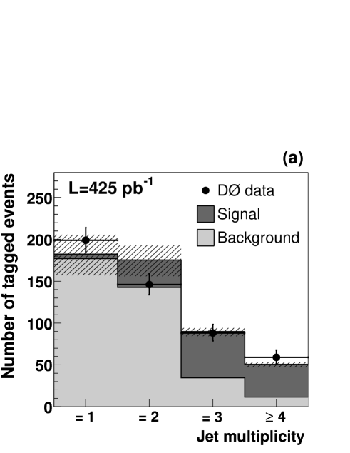
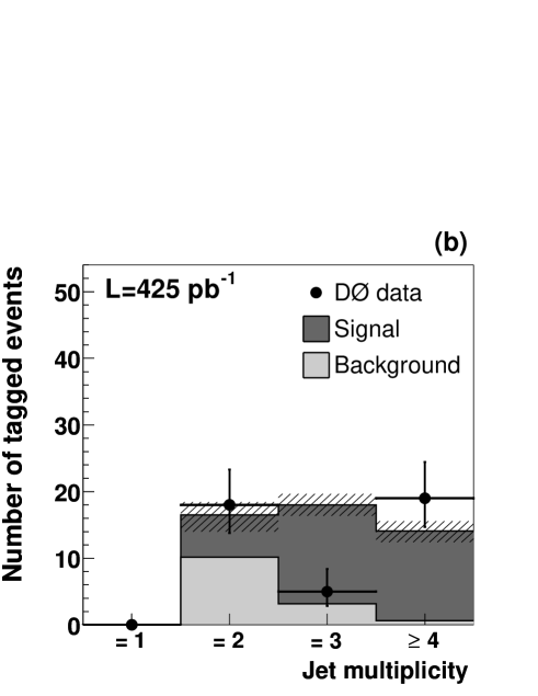
Figure 12: Observed number of tagged events in data compared to the total SM prediction for (a) single tagged events and (b) double tagged events. The number of $t\overline{t}$ events shown is calculated assuming a cross section of $6.6\;\rm pb$. The total uncertainty is represented by the hatched band.

The numbers of observed and predicted single and double tagged events are summarized in Tables 9 and 10, respectively. Figure 11 shows the observed number of tagged events in data compared to the total SM background predictions, excluding $t\overline{t}$. The background in the first jet multiplicity bin is dominated by $W$+light and $Wc$ events. The contribution from heavy flavor production, particularly from $Wb\bar{b}$, dominates for events with three or more jets. Very good agreement between observation and background prediction is observed in the background-dominated first and second jet multiplicity bins, which gives confidence in the background estimate of the analysis. A clear excess of observed events over background is seen in the third and fourth jet multiplicity bins. The excess events are attributed to $t\overline{t}$ production and are used to extract the cross section. Figure 12 shows the observed number of tagged events in data compared to the total SM predictions including $t\overline{t}$. The number of $t\overline{t}$ events shown is calculated based on the measured cross section.

	$e$+jets								$\mu$+jets
	1 jet		2 jets		3 jets		$\geq$4 jets		1 jet		2 jets		3 jets		$\geq$4 jets
$W$+light	20.9$\pm$	0.7	10.1$\pm$	0.7	2.45$\pm$	0.19	0.59$\pm$	0.13	24.9$\pm$	0.8	13.2$\pm$	0.8	2.63$\pm$	0.19	0.46$\pm$	0.11
$W(c\bar{c})$	6.6$\pm$	0.1	3.7$\pm$	0.2	0.88$\pm$	0.06	0.26$\pm$	0.06	7.5$\pm$	0.1	4.3$\pm$	0.1	0.90$\pm$	0.06	0.24$\pm$	0.06
$W(b\bar{b})$	18.8$\pm$	0.3	9.6$\pm$	0.3	2.25$\pm$	0.16	0.58$\pm$	0.12	21.6$\pm$	0.4	10.9$\pm$	0.3	2.32$\pm$	0.15	0.50$\pm$	0.12
$Wc$	24.3$\pm$	0.5	11.2$\pm$	0.4	1.53$\pm$	0.12	0.24$\pm$	0.05	27.6$\pm$	0.5	12.0$\pm$	0.4	1.56$\pm$	0.11	0.19$\pm$	0.04
$Wc\bar{c}$			4.9$\pm$	0.2	1.39$\pm$	0.15	0.40$\pm$	0.09			5.6$\pm$	0.2	1.62$\pm$	0.13	0.34$\pm$	0.08
$Wb\bar{b}$			10.1$\pm$	0.3	3.00$\pm$	0.22	0.70$\pm$	0.15			11.1$\pm$	0.3	3.05$\pm$	0.21	0.58$\pm$	0.13
$W$+jets	70.6$\pm$	0.9	49.6$\pm$	0.9	11.5$\pm$	0.4	2.77$\pm$	0.26	81.6$\pm$	1.0	57.1$\pm$	1.0	12.1$\pm$	0.4	2.31$\pm$	0.23
QCD	6.8$\pm$	1.5	10.0$\pm$	1.7	5.2$\pm$	1.2	2.95$\pm$	0.98	7.2$\pm$	1.3	5.8$\pm$	1.3	1.57$\pm$	0.89	2.77$\pm$	1.02
Single top	3.30$\pm$	0.07	7.3$\pm$	0.1	1.88$\pm$	0.06	0.30$\pm$	0.03	2.65$\pm$	0.05	6.5$\pm$	0.1	1.72$\pm$	0.04	0.27$\pm$	0.02
Diboson	2.26$\pm$	0.10	2.75$\pm$	0.11	0.23$\pm$	0.03	$<0.01$		2.28$\pm$	0.10	2.94$\pm$	0.11	0.22$\pm$	0.03	$<0.01$
$Z/\gamma^{*}\rightarrow\tau^{+}\tau^{-}$	0.15$\pm$	0.04	0.40$\pm$	0.07	0.03$\pm$	0.01	$<0.01$		0.19$\pm$	0.07	0.29$\pm$	0.05	0.09$\pm$	0.05	0.01$\pm$	0.02
$N_{\text{bkg}}$	83.1$\pm$	1.7	70.1$\pm$	2.0	18.8$\pm$	1.4	6.0$\pm$	1.1	93.9$\pm$	1.7	72.6$\pm$	1.7	15.7$\pm$	1.1	5.4$\pm$	1.1
Syst.	+10.7$-$11.8		+8.5$-$9.0		+1.9$-$2.0		+0.5$-$0.5		+12.2$-$13.4		+9.3$-$9.9		+2.0$-$2.1		+0.4$-$0.4
$t\bar{t}\rightarrow l$+jets	1.07$\pm$	0.18	11.7$\pm$	0.3	27.3$\pm$	0.4	19.8$\pm$	0.3	0.60$\pm$	0.19	8.0$\pm$	0.4	23.6$\pm$	0.4	18.8$\pm$	0.4
$t\bar{t}\rightarrow ll$	2.28$\pm$	0.04	7.1$\pm$	0.1	2.34$\pm$	0.04	0.33$\pm$	0.02	1.60$\pm$	0.03	5.9$\pm$	0.1	2.18$\pm$	0.04	0.29$\pm$	0.01
$N_{\text{pred}}$	86.5$\pm$	1.7	88.9$\pm$	2.0	48.5$\pm$	1.4	26.2$\pm$	1.1	96.1$\pm$	1.7	86.5$\pm$	1.7	41.5$\pm$	1.1	24.5$\pm$	1.1
Syst.	+10.7$-$11.9		+8.3$-$10.4		+2.0$-$3.3		+1.0$-$3.5		+12.3$-$13.4		+9.8$-$9.8		+2.2$-$2.5		+2.6$-$1.0
$N_{\text{obs}}$	94		78		47		33		105		68		41		26

Table 9: Summary of observed ($N_{\text{obs}}$) and predicted ($N_{\text{pred}})$ numbers of single tagged events in the $e$+jets and the $\mu$+jets channels. Uncertainties shown are statistical; the systematic uncertainties are included in the row labeled Syst. The number of $t\overline{t}$ events quoted is calculated assuming a cross section of $6.6\;\rm pb$.

	$e$+jets						$\mu$+jets
	2 jets		3 jets		$\geq$4 jets		2 jets		3 jets		$\geq$4 jets
$W$+light	0.017$\pm$	0.003	$<0.01$		$<0.01$		0.027$\pm$	0.003	$<0.01$		$<0.01$
$W(c\bar{c})$	0.014$\pm$	0.002	$<0.01$		$<0.01$		0.019$\pm$	0.003	$<0.01$		$<0.01$
$W(b\bar{b})$	0.13$\pm$	0.03	0.06$\pm$	0.01	$<0.01$		0.29$\pm$	0.05	0.05$\pm$	0.01	0.02$\pm$	0.01
$Wc$	0.027$\pm$	0.002	$<0.01$		$<0.01$		0.039$\pm$	0.003	$<0.01$		$<0.01$
$Wc\bar{c}$	0.24$\pm$	0.01	0.07$\pm$	0.01	0.02$\pm$	0.01	0.28$\pm$	0.01	0.09$\pm$	0.01	0.02$\pm$	0.01
$Wb\bar{b}$	2.80$\pm$	0.13	0.86$\pm$	0.08	0.22$\pm$	0.05	3.30$\pm$	0.14	0.87$\pm$	0.07	0.17$\pm$	0.04
$W$+jets	3.23$\pm$	0.13	1.00$\pm$	0.08	0.26$\pm$	0.05	3.96$\pm$	0.15	1.02$\pm$	0.08	0.22$\pm$	0.04
QCD	$<0.01$		0.27$\pm$	0.22	$<0.01$		0.26$\pm$	0.29	$<0.01$		$<0.01$
Single top	1.07$\pm$	0.02	0.39$\pm$	0.02	0.07$\pm$	0.01	0.93$\pm$	0.01	0.37$\pm$	0.01	0.07$\pm$	0.01
Diboson	0.34$\pm$	0.02	0.04$\pm$	0.01	$<0.01$		0.26$\pm$	0.02	0.03$\pm$	0.01	$<0.01$
$Z\rightarrow\tau^{+}\tau^{-}$	$<0.01$		$<0.01$		$<0.01$		$<0.01$		0.02$\pm$	0.02	$<0.01$
$N_{\text{bkg}}$	4.64$\pm$	0.28	1.70$\pm$	0.40	0.34$\pm$	0.29	5.42$\pm$	0.33	1.44$\pm$	0.34	0.29$\pm$	0.38
Syst.	+0.83$-$0.81		+0.26$-$0.25		+0.06$-$0.06		+0.99$-$0.97		+0.27$-$0.25		+0.05$-$0.06
$t\bar{t}\rightarrow l$+jets	1.72$\pm$	0.19	7.3$\pm$	0.3	6.9$\pm$	0.2	1.02$\pm$	0.15	6.2$\pm$	0.3	6.3$\pm$	0.3
$t\bar{t}\rightarrow ll$	1.81$\pm$	0.02	0.65$\pm$	0.01	0.09$\pm$	0.01	1.50$\pm$	0.02	0.61$\pm$	0.01	0.08$\pm$	0.01
$N_{\text{pred}}$	8.2$\pm$	0.3	9.7$\pm$	0.4	7.3$\pm$	0.3	7.9$\pm$	0.4	8.3$\pm$	0.3	6.7$\pm$	0.4
Syst.	+0.8$-$1.9		+0.6$-$1.3		+0.4$-$1.8		+1.3$-$1.0		+1.3$-$0.7		+1.7$-$0.4
$N_{\text{obs}}$	12		2		11		6		3		8

Table 10: Summary of observed ($N_{\text{obs}}$) and predicted ($N_{\text{pred}})$ numbers of double tagged events in the $e$+jets and the $\mu$+jets channels. Uncertainties shown are statistical; the systematic uncertainties are included in the row labeled Syst. The number of $t\overline{t}$ events quoted is calculated assuming a cross section of $6.6\;\rm pb$.

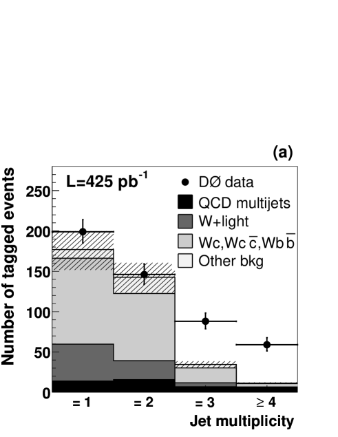
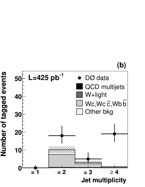
Figure 11: Observed number of tagged events in data compared to the total SM background predictions (excluding $t\overline{t}$) for (a) single tagged events and (b) double tagged events. The total uncertainty on the background prediction is represented by the hatched band. The excess of observed events in the third and fourth jet multiplicity bins is attributed to $t\overline{t}$ production.

IX Cross Section Result

The $t\overline{t}$ production cross section is extracted from the excess of tagged events over background expectation according to:

$$\sigma=\frac{N_{\text{obs}}-N_{\text{bkg}}}{Br\cdot{\mathcal{L}}\cdot\varepsilon_{\text{presel}}\cdot P^{\text{tag}}}\;,$$

where $Br$ is the branching ratio of the considered final state, $\mathcal{L}$ is the integrated luminosity, $\varepsilon_{\text{presel}}$ is the $t\overline{t}$ preselection efficiency, and $P^{\text{tag}}$ is the probability for a $t\overline{t}$ event to have one or more jets identified as $b$ jets.

The $t\overline{t}$ production cross section is calculated by performing a maximum likelihood fit to the observed number of events. The analysis is split into eight different channels: $e$+3 jets single tag, $e$+3 jets double tag, $e$+4 jets single tag, $e$+4 jets double tag, $\mu$+3 jets single tag, $\mu$+3 jets double tag, $\mu$+4 jets single tag, and $\mu$+4 jets double tag. The resulting cross sections are given for the electron and the muon channels separately and combined. If the index $\gamma$ refers to one of the eight channels, the likelihood ${\mathcal{L}}_{1}$ to observe $N^{\text{obs}}_{\gamma}$ for a cross section $\sigma_{t\bar{t}}$ is proportional to

$${\mathcal{L}}_{1} = \prod_{\gamma}{\mathcal{P}}[N^{\mathrm{obs}}_{\gamma},N^{\mathrm{pred}}_{\gamma}(\sigma_{t\bar{t}})]\,.$$ (3)

${\mathcal{P}}(n,\mu)=\frac{\mu^{n}\mathrm{e}^{-\mu}}{n\mathrm{!}}$ generically denotes the Poisson probability function for $n$ observed events, given an expectation of $\mu$ events. The predicted number of events in each channel is the sum of the predicted number of background events and the number of expected $t\overline{t}$ events. Both the number of $W$+jets events before tagging and the number of expected $t\overline{t}$ events are functions of the $t\overline{t}$ cross section that is being determined. For each iteration of the maximization procedure of the likelihood, the number of $t\overline{t}$ events in the untagged sample is calculated and the number of $W$+jets is rederived. A detailed explanation of the treatment of the event statistics in the cross section calculation can be found in Appendix B.

The final cross section is determined using a nuisance parameter likelihood method nuisance that incorporates all systematic uncertainties in the fit in such a way that allows them to affect the central value of the cross section. In this approach, each independent source of systematic uncertainty is modeled by a free parameter. Each nuisance parameter is modeled with a Gaussian centered on zero and with a standard deviation of one. The nuisance parameters are allowed to change the central values of all efficiencies, tagging probabilities, and flavor fractions, which are allowed to vary within their uncertainties. The correlations are taken into account in a natural way, by letting the same nuisance parameter affect different variables. The total likelihood function that is maximized is the product of ${\mathcal{L}}_{1}$ and ${\mathcal{L}}_{2}$, with

$${\mathcal{L}}_{2}=\prod_{i}{\mathcal{G}}(\nu_{i};0,1)\,,$$

where ${\mathcal{G}}(\nu_{i};0,1)$ is the normal probability of the nuisance parameter $i$ to take the value $\nu_{i}$.

The measured $t\bar{t}$ production cross sections for a top quark mass of $175\;\rm GeV$ are

$$\mu+{\rm jets} : \quad\sigma_{t\overline{t}}=6.1^{+1.3}_{-1.2}{\rm(stat+syst)}\>\pm 0.4\>{\rm(lum)}\>{\rm pb},$$

$$e+{\rm jets} : \quad\sigma_{t\overline{t}}=6.9^{+1.4}_{-1.2}{\rm(stat+syst)}\>\pm 0.4\>{\rm(lum)}\>{\rm pb},$$

$$l+{\rm jets} : \quad\sigma_{t\overline{t}}=6.6\pm 0.9{\rm(stat+syst)}\>\pm 0.4\>{\rm(lum)}\>{\rm pb}.$$

The first uncertainty corresponds to the combined statistical and systematic uncertainties, and the second one to the luminosity error of $\pm 6.1\%$.

A complete list of systematic uncertainties is given in Table 11, where a cross indicates if the background normalization ($\Delta b$) and/or the $t\bar{t}$ efficiency ($\Delta\varepsilon$) are affected within a given channel. The systematic uncertainties have been classified as uncorrelated (usually of statistical origin in either MC or data) or correlated. The correlation can be between channels (i.e. $e$+jets and $\mu$+jets) and/or between jet multiplicity bins ($N_{\text{jet}}=3$ and $N_{\text{jet}}\geq 4$) within a particular channel. All systematic uncertainties are fully correlated between the single and double tagged samples.

		e+jets		$\mu$+jets
		$\Delta b$	$\Delta\varepsilon$	$\Delta b$	$\Delta\varepsilon$
	Muon trigger			$\times$	$\times$
	EM trigger	$\times$	$\times$
	Muon preselection			$\times$	$\times$
	Electron preselection	$\times$	$\times$
	Preselection efficiency (MC statistics)		$\times$		$\times$
	$\varepsilon_{\text{QCD}}$ and $\varepsilon_{\text{sig}}$	$\times$		$\times$
	Matrix method (data statistics)	$\times$	$\times$	$\times$	$\times$
	$W$ fractions (MC statistics)	$\times$		$\times$
	Jet trigger	$\times$	$\times$	$\times$	$\times$
	Jet preselection	$\times$	$\times$	$\times$	$\times$
	Taggability in data	$\times$	$\times$	$\times$	$\times$
	Flavor dependence of taggability	$\times$	$\times$	$\times$	$\times$
	Semileptonic $b$ tagging efficiency in data	$\times$	$\times$	$\times$	$\times$
	Semileptonic $b$ tagging efficiency in MC	$\times$	$\times$	$\times$	$\times$
	Inclusive $b$ tagging efficiency in MC	$\times$	$\times$	$\times$	$\times$
	Inclusive $c$ tagging efficiency in MC	$\times$	$\times$	$\times$	$\times$
	Negative tagging efficiency in data	$\times$	$\times$	$\times$	$\times$
	$SF_{ll}$ and $SF_{hf}$	$\times$	$\times$	$\times$	$\times$
	$W$ fractions	$\times$		$\times$

Table 11: Summary of systematic uncertainties affecting the signal efficiency and/or background prediction. The labels correlated and uncorrelated refer to the $\mu$+jets and $e$+jets channels.

The nuisance parameter likelihood provides the total uncertainty on the cross section including contributions from systematic and statistical origin. To estimate the contribution of each individual systematic source, all but the corresponding nuisance parameter are fixed in the fit, and the maximization is redone. The statistical contribution is then deconvoluted from the obtained uncertainty to extract the contribution for that particular source. The resulting systematic uncertainties are summarized in Table 12.

The total uncertainty, excluding luminosity, is $\approx 14\%$. The main contribution of $\approx 11\%$ is statistical; the remaining $\approx 8\%$ is due to systematic effects. The primary contribution to the systematic uncertainties arises from the semileptonic $b$ tagging efficiency measured in data. The second largest source of systematic uncertainty originates from the matching of $W$ fractions and higher-order effects.

Source	$\sigma^{+}$	$\sigma^{-}$
Muon trigger	0.05	0.07
EM trigger	0.00	0.01
Jet trigger	0.00	0.01
Muon preselection	0.16	0.14
Electron preselection	0.17	0.15
Jet preselection	0.13	0.11
Preselection efficiency (MC statistics)	0.06	0.04
$\varepsilon_{\mathrm{QCD}}$ and $\varepsilon_{\mathrm{sig}}$ in $\mu$+jets channel	0.04	0.03
$\varepsilon_{\mathrm{QCD}}$ and $\varepsilon_{\mathrm{sig}}$ in $e$+jets channel	0.06	0.00
Matrix Method (data statistics)	0.15	0.15
Taggability in data	0.03	0.00
Flavor dependence of taggability	0.00	0.03
Semileptonic $b$ tagging efficiency in data	0.33	0.24
Semileptonic $b$ tagging efficiency in MC	0.17	0.04
Inclusive $b$ tagging efficiency in MC	0.00	0.00
Inclusive $c$ tagging efficiency in MC	0.01	0.00
Negative tagging efficiency in data	0.00	0.01
$SF_{ll}$ and $SF_{hf}$	0.01	0.00
$W$ fractions	0.29	0.27
$W$ fractions (MC statistics)	0.03	0.03
Total systematics (quad sum of the above)	0.57	0.47
Total uncertainty (nuisance parameter lhood)	0.94	0.86

Table 12: Systematic uncertainties in the combined $l$+jets channel.

The measured cross section depends on the assumed mass of the top quark $m_{t}$. The dependence was studied by repeating the analysis on MC $t\overline{t}$ samples generated at different values of $m_{t}$. The resulting dependence can be parameterized as $\sigma_{t\overline{t}}(m_{t})=0.000273m_{t}^{2}-0.145m_{t}+23.5$ for the central value, $-0.00704m_{t}+2.26$ for the $+1\sigma$ uncertainty, and $0.00687m_{t}-2.17$ for the $-1\sigma$ uncertainty. The dependence is shown in Fig. 13.

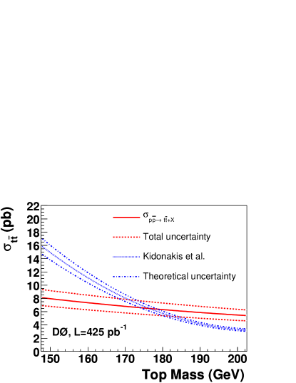
Figure 13: Top quark mass dependence of the measured cross section compared to the theoretical prediction theoxsec .

X Conclusions

A measurement of the $t\overline{t}$ production cross section in $p\overline{p}$ collisions at a center of mass energy of 1.96 TeV is presented in events with a lepton, a neutrino, and $\geq 3$ jets. After a preselection of the objects in the final state, a lifetime $b$ tagging algorithm which explicitly reconstructs secondary vertices is applied, removing approximately 95% of the background while keeping 60% of the $t\overline{t}$ signal. The measurement combines the $\mu$+jets and the $e$+jets channels, using 422 pb^-1 and 425 pb^-1 of data, respectively. The measured $t\overline{t}$ production cross section for a top quark mass of $175\;\rm GeV$ is

$$\sigma_{p\overline{p}\rightarrow t\overline{t}+X}=6.6\pm 0.9\>{\rm(stat+syst)}\>\pm 0.4\>{\rm(lum)}\>{\rm pb}\,,$$

in good agreement with SM expectations. The systematic uncertainty on the result (excluding luminosity) is $\approx 8$%. This represents a factor of three reduction in the systematic uncertainty compared to previous publications by the D0 collaboration D0Run2 , making this result the most precise D0 measurement of the $t\overline{t}$ production cross section to date.

We thank the staffs at Fermilab and collaborating institutions, and acknowledge support from the DOE and NSF (USA); CEA and CNRS/IN2P3 (France); FASI, Rosatom and RFBR (Russia); CAPES, CNPq, FAPERJ, FAPESP and FUNDUNESP (Brazil); DAE and DST (India); Colciencias (Colombia); CONACyT (Mexico); KRF and KOSEF (Korea); CONICET and UBACyT (Argentina); FOM (The Netherlands); PPARC (United Kingdom); MSMT (Czech Republic); CRC Program, CFI, NSERC and WestGrid Project (Canada); BMBF and DFG (Germany); SFI (Ireland); The Swedish Research Council (Sweden); Research Corporation; Alexander von Humboldt Foundation; and the Marie Curie Program.

Appendix A Monte Carlo generation of $W$+jets events

The $W$+jets background is simulated using alpgen 1.3 alpgen followed by pythia 6.2 pythia to simulate the underlying event and the hadronization. The samples are generated separately for processes with 1, 2, 3, and 4 or more partons in the final state, as summarized in Table 13. No parton-level cuts are applied on the heavy quarks ($c$ or $b$) except for the $c$ quark in the single $c$ quark production process; the correct masses for the $c$ and the $b$ quark are also included. The processes $Wc\bar{c}c\bar{c}$, $Wb\bar{b}c\bar{c}$, and $Wb\bar{b}b\bar{b}$ are not included as their cross sections are negligible. $W$ bosons are forced to decay to leptons; taus are subsequently forced to decay leptonically using tauola. The respective fraction of $W{\rightarrow}\tau\nu$ events is adjusted in the overall sample to correctly reflect its contributions to the $e$+jets and $\mu$+jets channels.

Process	$\sigma$(pb)	Process	$\sigma$(pb)	Process	$\sigma$(pb)	Process	$\sigma$(pb)
$Wj$	1600	$Wjj$	517	$Wjjj$	163	$Wjjjj$	49.5
$Wc$	51.8	$Wcj$	28.6	$Wcjj$	19.4	$Wcjjj$	3.15
		$Wb\bar{b}$	9.85	$Wb\bar{b}J$	5.24	$Wb\bar{b}Jj$	2.86
		$Wc\bar{c}$	24.3	$Wc\bar{c}J$	12.5	$Wc\bar{c}Jj$	5.83

Table 13: $W$+jets boson processes in alpgen and their cross sections for the leptonic $W$ boson decay, $\sigma\equiv\sigma_{p\overline{p}\rightarrow W+\text{jets}}Br(W\rightarrow l\nu)$, where $j$ =$u$,$d$,$s$,$g$ and $J$ =$u$,$d$,$s$,$g$,$c$.

The leading-order parton level calculations performed by alpgen need to be consistently combined with the partonic evolution given by the shower MC program pythia to avoid the double counting of configurations leading to the same final state. An approximation of the MLM matching Mangano (referred to as ad hoc matching) is used in the present analysis, where the matching is performed between matrix element partons and reconstructed jets. The $W$+jets MC samples are used in the analysis according to the number of heavy flavor ($c$ or $b$) jets in the final state, classified as follows: $W+$ light denotes events without $c$ or $b$ jets; $Wc$ denotes events with one $c$ jet due to single $c$ production; $W(c\bar{c})$ denotes events with one $c$ jet due to double $c$ production where two $c$ quarks are merged in one jet or one of the $c$ jets is outside of the acceptance region; $Wc\bar{c}$ denotes events with two $c$ jets; $W(b\bar{b})$ denotes events with one $b$ jet due to double $b$ production where two $b$ quarks are merged in one jet or one of the $b$ jets is outside of the acceptance region (single $b$ production is highly suppressed and neglected); and $Wb\bar{b}$ denotes events with two $b$ jets. Events are kept in the sample if the number of reconstructed jets equals the number of matrix element partons, where $(c\bar{c})$ and $(b\bar{b})$ are treated as one parton. As the fourth jet multiplicity bin is treated inclusively in the analysis, all events with $\geq 4$ reconstructed jets are kept, independently of the number of additional non-matched light jets.

Appendix B Handling of the Event Statistics uncertainties

The matrix method (see Sec. VI) is used three times in this analysis: to determine the number of $W$-like and QCD multijet events in the preselected, the single, and the double tagged samples. The number of observed events used by the matrix method is subject to random fluctuations according to Poisson statistics and contributes to the total statistical uncertainty on the cross section measurement. To treat these uncertainties properly, each number of events entering the matrix method is considered as a free parameter constrained to its observed value. This appendix details the treatment of statistical uncertainties arising from the number of events observed in data in the extraction of the cross section.

For the preselected samples, the matrix method gives the number of $W$-like $N^{\text{sig}}$ and QCD multijet $N^{\text{QCD}}$ events in the tight preselected sample as

$$N^{\text{sig}}_{t}=\varepsilon_{\text{sig}}\frac{N_{t}-\varepsilon_{\text{QCD}}N_{\ell}}{\varepsilon_{\text{sig}}-\varepsilon_{\text{QCD}}},$$

$$N^{\text{QCD}}_{t}=\varepsilon_{\text{QCD}}\frac{\varepsilon_{\text{sig}}N_{\ell}-N_{t}}{\varepsilon_{\text{sig}}-\varepsilon_{\text{QCD}}}.$$

The true values $N_{\ell}$ and $N_{t}$ are not known, and are left floating in the cross section calculation but constrained to their measured values $\tilde{N}_{\ell}$ and $\tilde{N}_{t}$ using Poisson statistics.

It is necessary to take into account that $N_{\ell}$ and $N_{t}$ are not independent variables. To do so, the matrix method equations are expressed in terms of $N_{t}$ and $N_{\ell-t}$, the latter representing the number of events that are loose but not tight. The equations become

$$N^{\text{sig}}_{t}=\varepsilon_{\text{sig}}\frac{N_{t}-\varepsilon_{\text{QCD}}(N_{t}+N_{\ell-t})}{\varepsilon_{\text{sig}}-\varepsilon_{\text{QCD}}},$$

$$N^{\text{QCD}}_{t}=\varepsilon_{\text{QCD}}\frac{\varepsilon_{\text{sig}}(N_{t}+N_{\ell-t})-N_{t}}{\varepsilon_{\text{sig}}-\varepsilon_{\text{QCD}}}.$$

Here, $N_{t}$ and $N_{\ell-t}$ are constrained respectively to the observed number of tight events, and to the observed number of loose-but-not-tight events by adding the following factor to the likelihood function

$${\mathcal{P}}(\tilde{N}_{t};N_{t})\times{\mathcal{P}}(\tilde{N}_{\ell-t};N_{\ell-t}),$$

which represents the probability to observe $\tilde{N}_{t}$ and $\tilde{N}_{\ell-t}$ given their true values $N_{t}$ and $N_{\ell-t}$.

This procedure can be repeated for the single and double tagged samples to predict the number of QCD multijet events as

$$N_{\text{QCD}}^{\text{1tag}}=\varepsilon_{\text{QCD}}\frac{\varepsilon_{\text{sig}}(N^{\text{1tag}}_{\ell-t}+N^{\text{1tag}}_{t})-N^{\text{1tag}}_{t}}{\varepsilon_{\text{sig}}-\varepsilon_{\text{QCD}}},$$

$$N_{\text{QCD}}^{\text{2tag}}=\varepsilon_{\text{QCD}}\frac{\varepsilon_{\text{sig}}(N^{\text{2tag}}_{\ell-t}+N^{\text{2tag}}_{t})-N^{\text{2tag}}_{t}}{\varepsilon_{\text{sig}}-\varepsilon_{\text{QCD}}}.$$

Note that the number of tight events with one tag $N^{1\text{tag}}_{t}$ and the number of tight events with two tags $N^{2\text{tag}}_{t}$ correspond to $N^{\text{obs}}_{\gamma}$ in Eq. 3 in Sec. IX. Therefore, $N^{1\text{tag}}_{t}$ and $N^{2\text{tag}}_{t}$ are already constrained to their observed values and only one additional constraint for the number of events in the $\rm{loose}-{\rm tight}$ sample with one and two tags is needed:

$${\mathcal{P}}(\tilde{N}^{\text{1tag}}_{\ell-t};N^{\text{1tag}}_{\ell-t})\times{\mathcal{P}}(\tilde{N}^{\text{2tag}}_{\ell-t};N^{\text{2tag}}_{\ell-t}),$$

which represents the probability to observe $\tilde{N}^{1\text{tag}}_{\ell-t}$ and $\tilde{N}^{2\text{tag}}_{\ell-t}$ given their true values $N^{1\text{tag}}_{\ell-t}$ and $N^{2\text{tag}}_{\ell-t}$.

Both the tight and the $\rm{loose}-{\rm tight}$ sample can be separated into events with zero, one, or two tags. Let $N^{\text{0tag}}_{t}$ and $N^{\text{0tag}}_{\ell-t}$ represent the number of events with zero tags in the tight and the $\rm{loose}-{\rm tight}$ sample, respectively. During the maximization process, $N^{\text{0tag}}_{t}$ and $N^{\text{0tag}}_{\ell-t}$ are two free parameters that are constrained to their observed values with Poisson probabilities

$${\mathcal{P}}(\tilde{N}^{\text{0tag}}_{\ell-t};N^{\text{0tag}}_{\ell-t})\times{\mathcal{P}}(\tilde{N}^{\text{0tag}}_{t};N^{\text{0tag}}_{t}).$$

In addition, the number of predicted tagged events can be expressed in terms of the number of expected tagged events originating from $t\overline{t}$, QCD multijet, $W$+jets, and other small electroweak backgrounds, for one and two tags, respectively:

$$N^{1\text{tag}}_{t}=P^{1\text{tag}}_{t\bar{t}}N_{t\bar{t}}+N^{1\text{tag}}_{\text{QCD}}+P^{1\text{tag}}_{W}N_{W}+P^{1\text{tag}}_{\text{MC~{}bkg}}N_{\text{MC~{}bkg}},$$

$$N^{2\text{tag}}_{t}=P^{2\text{tag}}_{t\bar{t}}N_{t\bar{t}}+N^{2\text{tag}}_{\text{QCD}}+P^{2\text{tag}}_{W}N_{W}+P^{2\text{tag}}_{\text{MC~{}bkg}}N_{\text{MC~{}bkg}}.$$

The contribution from the small electroweak backgrounds (diboson, single top, and $Z\rightarrow\tau\tau$ production) is labeled MC bkg to indicate that its normalization before tagging is obtained from MC. $P^{1\text{tag}}_{\text{process}}$ and $P^{2\text{tag}}_{\text{process}}$ are the average event tagging probability for a certain process, for single and double tags, respectively.

The number of $W$+jets events in the preselected sample is given by

$$N_{W}=N_{t}^{\text{sig}}-N_{t\bar{t}}-N_{\text{MC~{}bkg}}.$$

Substituting this expression for $N_{W}$ into the equations for $N^{1\text{tag}}_{t}$ and $N^{2\text{tag}}_{t}$ above allows us to express the latter quantities as a function of the tagging probabilities; signal and background efficiencies used in the matrix method; MC prediction for the small electroweak processes; and the floating parameters $N^{0\text{tag}}_{t}$, $N^{0\text{tag}}_{\ell-t}$, $N^{1\text{tag}}_{\ell-t}$, and $N^{2\text{tag}}_{\ell-t}$. $N^{1\text{tag}}_{t}$ and $N^{2\text{tag}}_{t}$ are constrained to their observed values using Poisson statistics

$${\mathcal{P}}(\tilde{N}^{1\text{tag}}_{t};N^{1\text{tag}}_{t})\times{\mathcal{P}}(\tilde{N}^{2\text{tag}}_{t};N^{2\text{tag}}_{t}).$$

The resulting likelihood is given by ${\mathcal{L}}_{1}$ below. The index $i$ indicates the product over the channels $e$+3 jets, $e$+4 jets, $\mu$+3 jet, and $\mu$+4 jets, respectively.

$$\mathrm{{\mathcal{L}}}_{1}=\prod_{i} \{ {\mathcal{P}}(\tilde{N}^{0\text{tag}}_{t};N^{0\text{tag}}_{t})\times{\mathcal{P}}(\tilde{N}^{1\text{tag}}_{t};N^{1\text{tag}}_{t})$$

$$\times {\mathcal{P}}(\tilde{N}^{2\text{tag}}_{t};N^{2\text{tag}}_{t})\times{\mathcal{P}}(\tilde{N}^{0\text{tag}}_{\ell-t};N^{0\text{tag}}_{\ell-t})$$

$$\times {\mathcal{P}}(\tilde{N}^{1\text{tag}}_{\ell-t};N^{1\text{tag}}_{\ell-t})\times{\mathcal{P}}(\tilde{N}^{2\text{tag}}_{\ell-t};N^{2\text{tag}}_{\ell-t})\}\;.$$

References

- (1)
- (2) Visitor from Helsinki Institute of Physics, Helsinki, Finland.
- (3) F. Abe et al., CDF Collaboration, Phys. Rev. Lett. 74 2626 (1995).
- (4) S. Abachi et al., D0 Collaboration, Phys. Rev. Lett. 74 2632 (1995).
- (5) P. Nason, S. Dawson, and R. K. Ellis, Nucl. Phys. B 303, 607 (1988).
- (6) S. Catani, M. L. Mangano, P. Nason and L. Trentadue: Nucl. Phys. B 478, 273 (1996); Phys. Lett. B 378, 329 (1996).
- (7) N. Kidonakis and G. Sterman, Phys. Lett. B 387, 867 (1996) and Nucl. Phys. B 505, 321 (1997). R. Bonciani, S. Catani, M. L. Mangano, and P. Nason, Nucl. Phys. B 529, 424 (1998). N. Kidonakis, Phys. Rev. D 64, 014009 (2001). N. Kidonakis, E. Laenen, S. Moch, and R. Vogt, Phys. Rev. D 64, 114001 (2001). N. Kidonakis and R. Vogt,Phys. Rev. D 68, 114014 (2003).
- (8) N. Kidonakis and R. Vogt, Phys. Rev. D 68, 114014 (2003). M. Cacciari, S. Frixione, M. L. Mangano, P. Nason, and G. Ridolfi, JHEP 0404, 68 (2004).
- (9) D. Acosta et al., CDF Collaboration, Phys. Rev. Lett. 93, 142001 (2004); Phys. Rev. D 71, 052003 (2005); Phys. Rev. D 71, 072005 (2005); Phys. Rev. D 72, 032008 (2005); hep-ex/0603043 (2006), to be published in Phys. Rev. Lett.
- (10) V. M. Abazov et al., D0 Collaboration, Phys. Lett. B 626, 35 (2005).
- (11) V. M. Abazov et al., D0 Collaboration, Phys. Lett. B 626, 45 (2005).
- (12) V. M. Abazov et al., D0 Collaboration, Phys. Lett. B 626, 55 (2005).
- (13) S. Eidelman et al., Phys. Lett. B 592, 1 (2004).
- (14) “Measurement of the top quark pair production cross section in collisions at ”, D0 Collaboration Ph.D. thesis, Gustavo J. Otero y Garzón, University of Illinois at Chicago, March 2006.
- (15) V.M. Abazov et al., D0 Collaboration, “The upgraded D0 detector,” Nucl. Instr. and Methods A 565, 463 (2006).
- (16) T. Andeen et al., FERMILAB-TM-2365, in preparation.
- (17) R. Lipton, Nucl. Instr. and Methods A 418, 85 (1998).
- (18) J. Brzenziak et al., FERMILAB-TM-1886 (1994).
- (19) V.M. Abazov et al., Nucl. Instr. and Methods A 552, 372 (2005).
- (20) R. E. Kalman, J. Bas. Eng. 82, 35 (1960); R. E. Kalman and R. S. Brucy, J. Bas. Eng. 83, 95 (1961); P. Billoir, Nucl. Instrum. Meth. A 225, 352 (1984).
- (21) “Measurement of the Lifetime and Top Quark Identification using Secondary Vertex b-tagging”, D0 Collaboration Ph.D. thesis, Ariel Schartzman, Universidad de Buenos Aires, 2004.
- (22) We use the iterative, seed-based cone algorithm including midpoints, as described on p. 47 in G. C. Blazey et al., in Proceedings of the Workshop: “QCD and Weak Boson Physics in Run II,” edited by U. Baur, R. K. Ellis, and D. Zeppenfeld, Fermilab-Pub-00/297 (2000).
- (23) R. Brun, F. Carminati, CERN program library long writeup W5013, (1993).
- (24) M. L. Mangano, et al., hep-ph/0206293 (2003).
- (25) T. Sjöstrand, L. Lonnblad and S. Mrenna, hep-ph/0108264 (2001).
- (26) D. J. Lange, Nucl. Instrum. Meth. A 462, 152 (2001).
- (27) Z. Was and P. Golonka, arXiv:hep-ph/0411377 (2004).
- (28) A. Pukhov et al., arXiv:hep-ph/9908288 (1999).
- (29) J. M. Campbell and R. K. Ellis, Phys. Rev. D 60, 113006 (1999).
- (30) We give the name closure test to the comparison of the observation in a given sample with the prediction obtained using the parameterization derived in the same sample. We give the name validation test to the comparison of the observation in a given sample with the prediction obtained using the parameterization derived in a different sample.
- (31) The default Peterson fragmentation function in pythia is changed to the Bowler fragmentation function tuned to LEP/SLD results. Information about the Peterson fragmentation function can be found in C. Peterson, D. Schlatter, I. Schmitt, and P. Zerwas, Phys. Rev. D 27, 105 (1983). Information about the Bowler fragmentation function can be found in M. G. Bowler, Zeit. Phys. C 11, 169 (1981).
- (32) M. Mangano, http://mlm.home.cern.ch/mlm/alpgen/.
- (33) J. M. Campbell and R.K. Ellis, Phys. Rev. D 65, 113007 (2002).
- (34) J. M. Campbell and J. Houston, arXiv:hep-ph/0405276 (2004).
- (35) J. Huston, et al., JHEP 0207, 012 (2002).
- (36) P. Sinervo, in Proceedings of Statistical methods in Particle Physics, Astrophysics, and Cosmology, edited by L. Lyons, R. P. Mount, and R. Reitmeyer (SLAC, Stanford, 2003), p. 334.