EUROPEAN ORGANIZATION FOR NUCLEAR RESEARCH

OPAL PR417

CERN-EP-2006-XXX

July 13, 2006

Search for Invisibly Decaying Higgs Bosons
with Large Decay Width Using the
OPAL Detector at LEP

The OPAL Collaboration

Abstract

This paper describes a topological search for an invisibly decaying Higgs boson, $\mathrm{H}$, produced via the Bjorken process ($\mathrm{e}^{+}\mathrm{e}^{-}\to\mathrm{H}{}\mathrm{Z}$). The analysis is based on data recorded using the OPAL detector at LEP at centre-of-mass energies from 183 to 209 GeV corresponding to a total integrated luminosity of 629 pb^-1. In the analysis only hadronic decays of the Z boson are considered. A scan over Higgs boson masses from 1 to 120 GeV and decay widths from 1 to 3000 GeV revealed no indication for a signal in the data. From a likelihood ratio of expected signal and Standard Model background we determine upper limits on cross-section times branching ratio to an invisible final state. For moderate Higgs boson decay widths, these range from about 0.07 pb ($M_{\mathrm{H}}$ = 60 GeV) to 0.57 pb ($M_{\mathrm{H}}$ = 114 GeV). For decay widths above 200 GeV the upper limits are of the order of 0.15 pb. The results can be interpreted in general scenarios predicting a large invisible decay width of the Higgs boson. As an example we interpret the results in the so-called stealthy Higgs scenario. The limits from this analysis exclude a large part of the parameter range of this scenario experimentally accessible at LEP  2.

(To be submitted to Eur. Phys. J.)

The OPAL Collaboration

G. Abbiendi², C. Ainsley⁵, P.F. Åkesson⁷, G. Alexander²¹, G. Anagnostou¹, K.J. Anderson⁸, S. Asai²², D. Axen²⁶, I. Bailey²⁵, E. Barberio^7,p, T. Barillari³¹, R.J. Barlow¹⁵, R.J. Batley⁵, P. Bechtle²⁴, T. Behnke²⁴, K.W. Bell¹⁹, P.J. Bell¹, G. Bella²¹, A. Bellerive⁶, G. Benelli⁴, S. Bethke³¹, O. Biebel³⁰, O. Boeriu⁹, P. Bock¹⁰, M. Boutemeur³⁰, S. Braibant², R.M. Brown¹⁹, H.J. Burckhart⁷, S. Campana⁴, P. Capiluppi², R.K. Carnegie⁶, A.A. Carter¹², J.R. Carter⁵, C.Y. Chang¹⁶, D.G. Charlton¹, C. Ciocca², A. Csilling²⁸, M. Cuffiani², S. Dado²⁰, A. De Roeck⁷, E.A. De Wolf^7,s, K. Desch²⁴, B. Dienes²⁹, J. Dubbert³⁰, E. Duchovni²³, G. Duckeck³⁰, I.P. Duerdoth¹⁵, E. Etzion²¹, F. Fabbri², P. Ferrari⁷, F. Fiedler³⁰, I. Fleck⁹, M. Ford¹⁵, A. Frey⁷, P. Gagnon¹¹, J.W. Gary⁴, C. Geich-Gimbel³, G. Giacomelli², P. Giacomelli², M. Giunta⁴, J. Goldberg²⁰, E. Gross²³, J. Grunhaus²¹, M. Gruwé⁷, A. Gupta⁸, C. Hajdu²⁸, M. Hamann²⁴, G.G. Hanson⁴, A. Harel²⁰, M. Hauschild⁷, C.M. Hawkes¹, R. Hawkings⁷, G. Herten⁹, R.D. Heuer²⁴, J.C. Hill⁵, D. Horváth^28,c, P. Igo-Kemenes¹⁰, K. Ishii²², H. Jeremie¹⁷, P. Jovanovic¹, T.R. Junk^6,i, J. Kanzaki^22,u, D. Karlen²⁵, K. Kawagoe²², T. Kawamoto²², R.K. Keeler²⁵, R.G. Kellogg¹⁶, B.W. Kennedy¹⁹, S. Kluth³¹, T. Kobayashi²², M. Kobel^3,t, S. Komamiya²², T. Krämer²⁴, A. Krasznahorkay Jr.^29,e, P. Krieger^6,l, J. von Krogh¹⁰, T. Kuhl²⁴, M. Kupper²³, G.D. Lafferty¹⁵, H. Landsman²⁰, D. Lanske¹³, D. Lellouch²³, J. Letts^o, L. Levinson²³, J. Lillich⁹, S.L. Lloyd¹², F.K. Loebinger¹⁵, J. Lu^26,b, A. Ludwig^3,t, J. Ludwig⁹, W. Mader^3,t, S. Marcellini², A.J. Martin¹², T. Mashimo²², P. Mättig^m, J. McKenna²⁶, R.A. McPherson²⁵, F. Meijers⁷, W. Menges²⁴, F.S. Merritt⁸, H. Mes^6,a, N. Meyer²⁴, A. Michelini², S. Mihara²², G. Mikenberg²³, D.J. Miller¹⁴, W. Mohr⁹, T. Mori²², A. Mutter⁹, K. Nagai¹², I. Nakamura^22,v, H. Nanjo²², H.A. Neal³², R. Nisius³¹, S.W. O’Neale^1,∗, A. Oh⁷, M.J. Oreglia⁸, S. Orito^22,∗, C. Pahl³¹, G. Pásztor^4,g, J.R. Pater¹⁵, J.E. Pilcher⁸, J. Pinfold²⁷, D.E. Plane⁷, O. Pooth¹³, M. Przybycień^7,n, A. Quadt³¹, K. Rabbertz^7,r, C. Rembser⁷, P. Renkel²³, J.M. Roney²⁵, A.M. Rossi², Y. Rozen²⁰, K. Runge⁹, K. Sachs⁶, T. Saeki²², E.K.G. Sarkisyan^7,j, A.D. Schaile³⁰, O. Schaile³⁰, P. Scharff-Hansen⁷, J. Schieck³¹, T. Schörner-Sadenius^7,z, M. Schröder⁷, M. Schumacher³, R. Seuster^13,f, T.G. Shears^7,h, B.C. Shen⁴, P. Sherwood¹⁴, A. Skuja¹⁶, A.M. Smith⁷, R. Sobie²⁵, S. Söldner-Rembold¹⁵, F. Spano^8,y, A. Stahl¹³, D. Strom¹⁸, R. Ströhmer³⁰, S. Tarem²⁰, M. Tasevsky^7,d, R. Teuscher⁸, M.A. Thomson⁵, E. Torrence¹⁸, D. Toya²², P. Tran⁴, I. Trigger^7,w, Z. Trócsányi^29,e, E. Tsur²¹, M.F. Turner-Watson¹, I. Ueda²², B. Ujvári^29,e, C.F. Vollmer³⁰, P. Vannerem⁹, R. Vértesi^29,e, M. Verzocchi¹⁶, H. Voss^7,q, J. Vossebeld^7,h, C.P. Ward⁵, D.R. Ward⁵, P.M. Watkins¹, A.T. Watson¹, N.K. Watson¹, P.S. Wells⁷, T. Wengler⁷, N. Wermes³, G.W. Wilson^15,k, J.A. Wilson¹, G. Wolf²³, T.R. Wyatt¹⁵, S. Yamashita²², D. Zer-Zion⁴, L. Zivkovic²⁰

¹School of Physics and Astronomy, University of Birmingham, Birmingham B15 2TT, UK
²Dipartimento di Fisica dell’ Università di Bologna and INFN, I-40126 Bologna, Italy
³Physikalisches Institut, Universität Bonn, D-53115 Bonn, Germany
⁴Department of Physics, University of California, Riverside CA 92521, USA
⁵Cavendish Laboratory, Cambridge CB3 0HE, UK
⁶Ottawa-Carleton Institute for Physics, Department of Physics, Carleton University, Ottawa, Ontario K1S 5B6, Canada
⁷CERN, European Organisation for Nuclear Research, CH-1211 Geneva 23, Switzerland
⁸Enrico Fermi Institute and Department of Physics, University of Chicago, Chicago IL 60637, USA
⁹Fakultät für Physik, Albert-Ludwigs-Universität Freiburg, D-79104 Freiburg, Germany
¹⁰Physikalisches Institut, Universität Heidelberg, D-69120 Heidelberg, Germany
¹¹Indiana University, Department of Physics, Bloomington IN 47405, USA
¹²Queen Mary and Westfield College, University of London, London E1 4NS, UK
¹³Technische Hochschule Aachen, III Physikalisches Institut, Sommerfeldstrasse 26-28, D-52056 Aachen, Germany
¹⁴University College London, London WC1E 6BT, UK
¹⁵Department of Physics, Schuster Laboratory, The University, Manchester M13 9PL, UK
¹⁶Department of Physics, University of Maryland, College Park, MD 20742, USA
¹⁷Laboratoire de Physique Nucléaire, Université de Montréal, Montréal, Québec H3C 3J7, Canada
¹⁸University of Oregon, Department of Physics, Eugene OR 97403, USA
¹⁹CCLRC Rutherford Appleton Laboratory, Chilton, Didcot, Oxfordshire OX11 0QX, UK
²⁰Department of Physics, Technion-Israel Institute of Technology, Haifa 32000, Israel
²¹Department of Physics and Astronomy, Tel Aviv University, Tel Aviv 69978, Israel
²²International Centre for Elementary Particle Physics and Department of Physics, University of Tokyo, Tokyo 113-0033, and Kobe University, Kobe 657-8501, Japan
²³Particle Physics Department, Weizmann Institute of Science, Rehovot 76100, Israel
²⁴Universität Hamburg/DESY, Institut für Experimentalphysik, Notkestrasse 85, D-22607 Hamburg, Germany
²⁵University of Victoria, Department of Physics, P O Box 3055, Victoria BC V8W 3P6, Canada
²⁶University of British Columbia, Department of Physics, Vancouver BC V6T 1Z1, Canada
²⁷University of Alberta, Department of Physics, Edmonton AB T6G 2J1, Canada
²⁸Research Institute for Particle and Nuclear Physics, H-1525 Budapest, P O Box 49, Hungary
²⁹Institute of Nuclear Research, H-4001 Debrecen, P O Box 51, Hungary
³⁰Ludwig-Maximilians-Universität München, Sektion Physik, Am Coulombwall 1, D-85748 Garching, Germany
³¹Max-Planck-Institute für Physik, Föhringer Ring 6, D-80805 München, Germany
³²Yale University, Department of Physics, New Haven, CT 06520, USA

^a and at TRIUMF, Vancouver, Canada V6T 2A3
^b now at University of Alberta
^c and Institute of Nuclear Research, Debrecen, Hungary
^d now at Institute of Physics, Academy of Sciences of the Czech Republic 18221 Prague, Czech Republic
^e and Department of Experimental Physics, University of Debrecen, Hungary
^f and MPI München
^g and Research Institute for Particle and Nuclear Physics, Budapest, Hungary
^h now at University of Liverpool, Dept of Physics, Liverpool L69 3BX, U.K.
ⁱ now at Dept. Physics, University of Illinois at Urbana-Champaign, U.S.A.
^j and Manchester University Manchester, M13 9PL, United Kingdom
^k now at University of Kansas, Dept of Physics and Astronomy, Lawrence, KS 66045, U.S.A.
^l now at University of Toronto, Dept of Physics, Toronto, Canada
^m current address Bergische Universität, Wuppertal, Germany
ⁿ now at University of Mining and Metallurgy, Cracow, Poland
^o now at University of California, San Diego, U.S.A.
^p now at The University of Melbourne, Victoria, Australia
^q now at IPHE Université de Lausanne, CH-1015 Lausanne, Switzerland
^r now at IEKP Universität Karlsruhe, Germany
^s now at University of Antwerpen, Physics Department,B-2610 Antwerpen, Belgium; supported by Interuniversity Attraction Poles Programme – Belgian Science Policy
^t now at Technische Universität, Dresden, Germany
^u and High Energy Accelerator Research Organisation (KEK), Tsukuba, Ibaraki, Japan
^v now at University of Pennsylvania, Philadelphia, Pennsylvania, USA
^w now at TRIUMF, Vancouver, Canada
^x now at DESY Zeuthen
^y now at CERN
^z now at DESY
^∗ Deceased

1 Introduction

An intense search for the Higgs boson was undertaken by all of the four LEP experiments in various Standard Model and non–Standard Model search channels. Searches for the Standard Model Higgs boson, exploiting the prediction for its decay modes and also searches for invisible Higgs boson decays as predicted by various extensions of the Standard Model excluded Higgs masses up to 114.4 GeV [1, 2]. These latter searches assumed a rather small invisible decay width comparable to the predicted Standard Model decay width for a light Higgs boson and well below the experimentally achievable mass resolution of about 3 to 5 GeV.

Recent theories that postulate the existence of additional spatial dimensions offer a new possibility for invisible Higgs decays [3]. In such theories the Planck mass is lowered to the TeV range and a rich spectrum of new particles appears, like graviscalars in the case of flat extra dimensions. Hence the Higgs boson can mix with the graviscalars, which leads to a missing energy signature in the detector [3]. This mixing can result in a large invisible decay width of the Higgs boson, depending on the model parameters, and would therefore alter the Standard Model branching ratios. As a consequence of the broadening of the Higgs resonance in the recoil mass spectrum, the signal-to-background ratio can deteriorate significantly. In a worst case scenario, searches optimised under the assumption of a narrow Higgs resonance might have missed the detection of a kinematically accessible Higgs boson at LEP.

This paper describes a search for the Higgs boson, H, which imposes no constraints on the total decay width. The Higgs boson is assumed to be produced in association with a Z boson via the Bjorken process, $\mathrm{e}^{+}\mathrm{e}^{-}\to\mathrm{H}{}\mathrm{Z}$, where the Z is required to decay hadronically and the invisible Higgs boson is detected as missing energy $E_{\mathrm{MIS}}$ in the event. The results are presented in a model-independent way in terms of limits on the Bjorken production cross-section times branching ratio, $\sigma(M_{\mathrm{H}},\Gamma_{\mathrm{H}})\times\mathrm{BR}(\mathrm{H}\to E_{\mathrm{MIS}})$, at a centre-of-mass energy of 206 GeV, where $\Gamma_{\mathrm{H}}$ is the Breit–Wigner width of the Higgs boson. A simple model extending the Standard Model with additional SU(3)${}_{\mathrm{C}}\times$SU(2)${}_{\mathrm{L}}\times$U(1)_Y singlet fields which interact strongly with the Higgs boson (“stealthy Higgs scenario” [4]) is chosen as an example for the interpretation of the result. This interaction gives rise to a large invisible decay width of the Higgs boson. This dedicated search expands on the previous decay-mode-independent search [5] carried out by the OPAL Collaboration which reported for the first time limits on the HZ production cross-section, interpreted in the stealthy Higgs model.

The paper is organised as follows. Section 2 introduces the stealthy Higgs scenario. Section 3 gives details about the modelling of signal and background. Section 4 describes the search and the results are interpreted in Section 5. We summarise the results in Section 6.

2 The stealthy Higgs scenario

In general renormalisable theories there might be other fundamental scalars, in addition to the Standard Model Higgs boson, that do not interact with normal matter. To investigate the influence of a hidden scalar sector on the Higgs observables the stealthy Higgs scenario conjectures the existence of additional SU(3)${}_{\mathrm{C}}\times$SU(2)${}_{\mathrm{L}}\times$U(1)_Y singlet fields called phions. Radiative corrections to weak processes are not sensitive to the presence of singlets in the theory because no Feynman graphs containing singlets appear at the one-loop level. Since effects at the two-loop level are below the experimental precision, the presence of a singlet sector is not ruled out by any LEP  1 precision data [4]. These phions would not interact via the strong or electro-weak forces, but couple only to the Higgs boson [4], thus offering invisible decay modes to the Higgs. The width of the Higgs resonance can become large if either the number of such singlets, $N$, or the coupling, $\omega$, is large, thus leading to a broad mass spectrum recoiling against the reconstructed Z boson.

Neglecting the fermionic part for the moment, the Lagrangian of the scalar sector in this model, adding only four new parameters to the Standard Model, is given by

$${\cal L}_{\mathrm{scalar}} = {\cal L}_{\mathrm{Higgs}}+{\cal L}_{\mathrm{phion}}+{\cal L}_{\mathrm{interaction}}$$ (1)

$${\cal L}_{\mathrm{Higgs}} = -\partial_{\mu}\phi^{\dagger}\partial^{\mu}\phi-\lambda\,(\phi^{\dagger}\phi-\frac{v^{2}}{2})^{2}$$ (2)

$${\cal L}_{\mathrm{phion}} = -\frac{1}{2}\,\partial_{\mu}\vec{\varphi}\,\partial^{\mu}\vec{\varphi}-\frac{1}{2}m_{\mathrm{phion}}^{2}\,\vec{\varphi}^{2}-\frac{\kappa}{8N}\,(\vec{\varphi}^{2})^{2}$$ (3)

$${\cal L}_{\mathrm{interaction}} = -\frac{\omega}{2\sqrt{N}}\,\,\vec{\varphi}^{2}\,\phi^{\dagger}\phi.$$ (4)

The term ${\cal L}_{\mathrm{Higgs}}$ describes the usual Standard Model Higgs doublet $\phi$ acquiring the Standard Model vacuum expectation value, $v$, and having its self-coupling $\lambda$. In the free Lagrangian of scalar singlets, ${\cal L}_{\mathrm{phion}}$, the singlets with mass $m_{\mathrm{phion}}$ are denoted as the O($N$)-symmetric multiplet $\vec{\varphi}$. The phions also have a self-coupling $\kappa$, which is fixed at $\kappa(2M_{\mathrm{Z}})=0$, to allow for the widest parameter range of the model. The self coupling term entering loop calculations is suppressed like 1/$N$. The interaction term between the Higgs and the additional phions, ${\cal L}_{\mathrm{interaction}}$, leads to the phenomenological consequence of invisible Higgs decays because the Higgs boson couples to the phions independently of their mass. The strength of the coupling is instead proportional to the coupling constant $\omega$, which is a free parameter of the model. Even though the vacuum-induced mass term of the phions after the symmetry-breaking is suppressed like $1/\sqrt{N}$ [4], the phions occur in loop corrections to the Higgs boson propagator and therefore affect the resonance width of the Higgs boson. An analytic expression [6] for the change in the Higgs width compared to the Standard Model decay width, $\Gamma_{\mathrm{SM}}$, can be found in the limit $N\to\infty$, when neglecting the self-coupling of the phions as a small effect:

$$\Gamma_{\mathrm{H}}(M_{\mathrm{H}})=\Gamma_{\mathrm{SM}}(M_{\mathrm{H}})+\frac{\omega^{2}v^{2}}{32\,\pi\,M_{\mathrm{H}}}\times\sqrt{1-4m_{\mathrm{phion}}^{2}/M_{\mathrm{H}}^{2}}.$$ (5)

The cross-section for the Bjorken process can be calculated from Equations 9 and 10 of reference [4]. Using the parametrisation for the invisible decay width (Equation 1 and 2 in  [7]) one can express the total cross-section for the production and invisible decay by

$$\sigma_{(\mathrm{e^{+}e^{-}}\rightarrow\mathrm{Z}+E_{\mathrm{MIS}})}=\int ds_{I}\,\sigma_{(\mathrm{e}^{+}\mathrm{e}^{-}\rightarrow\mathrm{ZH})}(s_{I})\,\frac{\sqrt{s_{I}}\quad\Gamma_{\mathrm{H}}^{\mathrm{inv}}}{\pi((M_{\mathrm{H}}^{2}-s_{I})^{2}+s_{I}\,\Gamma_{\mathrm{H}}^{2})}.$$ (6)

Here $s_{I}$ denotes the invariant mass squared of the invisible decay products of the Higgs boson. The production rate of these invisible masses is given by the Standard Model cross-section $\sigma_{(\mathrm{e}^{+}\mathrm{e}^{-}\rightarrow\mathrm{ZH})}(s_{I})$ for a Higgs boson of mass $\sqrt{s_{I}}$. Hence the Standard Model cross-section completely determines the dependence of the total cross-section on the centre-of-mass energy (see e.g. in [8]). Therefore the total cross-section goes rapidly to zero for Higgs boson masses above the kinematic limit. The effect of the convolution with the Breit-Wigner-like function is a broadening of the resonance in the recoil mass spectrum and hence a dilution of the signal-to-background ratio. In extreme cases of large invisible decay width one could expect the Higgs recoil mass spectrum to mimic the background. In such extreme cases even a light and kinematically accessible Higgs boson might have escaped detection at LEP.

In Section 5.2 we derive limits on the stealthy Higgs model under the assumption of $m_{\mathrm{phion}}=0$. By simulating signal spectra for different Higgs boson masses $M_{\mathrm{H}}$ and widths $\Gamma_{\mathrm{H}}$, we set limits in the $\omega$-$M_{\mathrm{H}}$ plane in the large $N$ limit.

3 Data sets and Monte Carlo samples

3.1 The OPAL detector and event reconstruction

The OPAL detector [9], operated between 1989 and 2000 at LEP, had nearly complete solid angle coverage and excellent hermeticity. The innermost detector of the central tracking was a high-resolution silicon microstrip vertex detector [10] which lay immediately outside the beam pipe. The silicon microvertex detector was surrounded by a high precision vertex drift chamber, a large volume jet chamber, and $z$–chambers which measured the $z$ coordinates of tracks, all in a uniform 0.435 T axial magnetic field. A lead-glass electromagnetic calorimeter with presampler was located outside the magnet coil. In combination with the forward calorimeters, a forward ring of lead-scintillator modules (the “gamma catcher”), a forward scintillating tile counter [9, 11], and the silicon-tungsten luminometer [12], the calorimeters provided a geometrical acceptance down to 25 mrad from the beam direction. The silicon-tungsten luminometer served to measure the integrated luminosity using small angle Bhabha scattering events [13]. The magnet return yoke was instrumented with streamer tubes and thin gap chambers for hadron calorimetry and is surrounded by several layers of muon chambers.

The analysis is based on data collected with the OPAL detector at LEP  2 from 1997 to 2000 at centre-of-mass energies between 183 and 209 GeV. The integrated luminosity analysed is 629.1 pb^-1. To compare with the Standard Model Monte Carlo the data are binned in five nominal centre-of-mass-energy points, corresponding to the energies at which the Monte Carlo is produced, as detailed in Table 1.

A fast online filtering algorithm classifies the events as multi-hadronic. Events are reconstructed from tracks and energy deposits (“clusters”) in the electromagnetic and hadronic calorimeters. All tracks and energy clusters satisfying quality requests similar to those described in [14] are associated to form “energy flow objects”. The measured energies are corrected for double counting of energy in the tracking chambers and calorimeters by the algorithm described in [14]. Global event variables, such as transverse momentum and visible mass, are then reconstructed from these objects and all events are forced into a two-jet topology using the Durham algorithm [15].

3.2 Signal and background modelling

To determine the detection efficiency for a signal from an invisibly decaying Higgs boson and the amount of expected background from Standard Model processes, several Monte Carlo samples are used. Signal events for a hypothetical Higgs boson mass $M_{\mathrm{H}}$ decaying with arbitrary broad width $\Gamma_{\mathrm{H}}$ are simulated by reweighting invisibly decaying events of type $\mathrm{H}\to\chi^{0}_{1}\chi^{0}_{1}$. The mass of neutralinos $\chi^{0}_{1}$ is chosen such that the Higgs boson with mass $m_{i}$ can decay into a pair of neutralinos, which leave the detector without being detected. These Higgs bosons with decays into ‘invisible’ particles are generated with masses $m_{i}$ from 1 GeV to 120 GeV with the HZHA [16] generator. The HZHA events are generated assuming the Standard Model production cross-section $\sigma_{(\mathrm{e}^{+}\mathrm{e}^{-}\rightarrow\mathrm{ZH})}$ for the Higgs boson. The test masses $m_{i}$ are spaced in steps of 1 GeV. The spacing of the test masses is chosen such that they are not resolved by the detector in the signal yielded after a reweighting procedure described in the following. From Equation 6 one extracts the event weights $w_{i}(m_{i};M_{\mathrm{H}},\Gamma_{\mathrm{H}})$ for a mass point $m_{i}$ contributing to the search for a Higgs boson of mass $M_{\mathrm{H}}$ and total decay width $\Gamma_{\mathrm{H}}$. The total decay width $\Gamma_{\mathrm{H}}$ is defined as the sum of Standard Model width and invisible width $\Gamma_{\mathrm{H}}^{\mathrm{inv}}$.

$$w_{i}(m_{i};M_{\mathrm{H}},\Gamma_{\mathrm{H}}) = \frac{\frac{d\sigma}{dm_{i}}(m_{i})}{\sum_{m_{j}=1\,\mathrm{GeV}}^{120\,\mathrm{GeV}}{\frac{d\sigma}{dm_{j}}(m_{j})}}$$ (7)

$$\frac{d\sigma}{dm_{i}}(m_{i}) = \frac{\sigma_{(\mathrm{e}^{+}\mathrm{e}^{-}\rightarrow\mathrm{ZH})}(m_{i})~{}2m_{i}^{2}\Gamma_{\mathrm{H}}^{\mathrm{inv}}}{\pi((M_{\mathrm{H}}^{2}-m^{2}_{i})^{2}+m^{2}_{i}\Gamma_{\mathrm{H}}^{2})}.$$ (8)

The Standard Model cross-section $\sigma_{(\mathrm{e}^{+}\mathrm{e}^{-}\rightarrow\mathrm{ZH})}$ for the Bjorken production process in Equation 8 propagates the centre-of-mass energy dependence of the total cross-section into the weights. The unweighted signal Monte Carlo samples contain 2000 events per mass point $m_{i}$. In the reweighted signal Monte Carlo sample all test masses contribute according to their weight. The reweighted masses $M_{\mathrm{H}}$ range from 1 to 120 GeV spaced in steps of 1 GeV. The smallest width simulated by this procedure is a $\Gamma_{\mathrm{H}}$ of 1 GeV and the largest a $\Gamma_{\mathrm{H}}$ of 3 TeV. The detection efficiency for a Higgs boson with $M_{\mathrm{H}}$ and $\Gamma_{\mathrm{H}}$ is estimated by the sum of selected event weights assuming binomial errors.

The classes of Standard Model background processes considered are two-photon, two- and four-fermion processes. For simulation of background processes the following generators are used: KK2F [17] and PYTHIA [18] (q$\bar{\mathrm{q}}(\gamma)$), GRC4F [19]  (four-fermion processes), PHOJET [20], HERWIG [21], Vermaseren [22] (hadronic and leptonic two-photon processes). For Monte Carlo generators other than HERWIG, the hadronisation is done using JETSET 7.4 [18]. The integrated luminosity of the main background Monte Carlo samples is at least 15 times the statistics of the data for the two-fermion background, 24 times for the four-fermion background and 30 times for the two-photon background. The Monte Carlo events are passed through a detailed simulation of the OPAL detector [23] and are reconstructed using the same algorithms as for the real data.

4 Search for $\mathrm{e}^{+}\mathrm{e}^{-}\to\mathrm{H}{}\mathrm{Z}$ with $\mathrm{Z}\to\mbox{$\mathrm{q}\bar{\mathrm{q}}$}$ and $\mathrm{H}\to E_{\mathrm{MIS}}$ final state

The event selection is intended to be efficient for the complete range of possible Higgs masses $M_{\mathrm{H}}$ and corresponding decay widths $\Gamma_{\mathrm{H}}$ studied in this search. The preselection cuts remain relatively loose because the final discrimination between signal and background is done by a likelihood-based selection. The optimised likelihood selection has to account for the fact that the kinematical properties of the signal change considerably over the range of masses and width hypotheses considered.

4.1 Event topologies

The signal signature is generally characterised by an acoplanar two-jet system from the Z boson decay. We use the term ‘acoplanar’ for jet pairs if the two jet axes and the beam axis are not consistent with lying in a single plane. The decay products of the Z boson are preferentially emitted into the central part of the detector, recoiling against the invisibly decaying Higgs boson. This is because, in contrast to the irreducible background of ZZ $\to\mbox{$\mathrm{q}\bar{\mathrm{q}}$}~{}\nu\overline{\nu}$ which is produced with an angular dependence of the differential cross-section proportional to $\cos^{2}\theta$, the Bjorken process is proportional to $\sin^{2}\theta$. The Higgs boson decay leads to a large missing momentum and a significant amount of missing energy. In two-photon processes, where the incoming electron and positron are scattered at low angles, usually one or both of the electrons remain undetected. Events of this type have large missing momentum with the missing momentum vector, $\vec{p}_{\mathrm{MIS}}$, pointing at low angles to the beam axis. The two-photon events have a small visible invariant mass $M_{\mathrm{VIS}}$ and a tiny transverse momentum $p^{\mathrm{T}}_{\mathrm{MIS}}$ but a considerable longitudinal momentum along the $z$-axis in the common case that the two photons do not have equal energy. Due to these special characteristics this background can be easily reduced to a negligible level.

The two-fermion background important for this search consists of $\mathrm{Z}/\gamma^{*}\to\mbox{$\mathrm{q}\bar{\mathrm{q}}$}(\gamma)$ events. These events tend to have a big cross-section if one or more initial state radiation photons (abbreviated as ISR photons) are emitted so that the effective centre-of-mass energy $\sqrt{s^{{}^{\prime}}}$ is reduced to a value near the Z-resonance (so-called radiative return events). The emission of ISR photons happens predominantly at small polar angles. In case of a mismeasurement or escape of the ISR photons through the beam pipe these events have a sizeable missing momentum preferentially oriented at small polar angles, close to the beam pipe. In such events the two jets are almost coplanar.

The most difficult background to separate is four-fermion processes with neutrinos in the final state, such as $\mathrm{W}^{+}\mathrm{W}^{-}$$\to\ell^{\pm}\nu$ $\mathrm{q}\bar{\mathrm{q}}$ and $W^{\pm}e^{\mp}\nu\to$ $\mathrm{q}\bar{\mathrm{q}}$$e^{\mp}\nu$ with the charged lepton escaping detection. The irreducible background to this search stems from ZZ $\to\nu\overline{\nu}\mbox{$\mathrm{q}\bar{\mathrm{q}}$}$ (about 28 % of all ZZ decays) leading to a signature indistinguishable from a signal event with a Higgs mass close to the Z boson mass. The vector bosons are usually not produced at rest, leading to a transverse momentum of the two-jet system and therefore to a large acoplanarity of the jets, as in the signal case. Furthermore, the missing momentum vector points into the central detector more often than for the two-fermion case. To discriminate between this background and the signal one can exploit the difference in the angular distribution of the differential production cross-section.

4.2 Preselection

The final discrimination between signal and background is made using a likelihood selection. Therefore the preselection cuts remain relatively loose. From cut No.(5) onwards the cut values have been tuned at a centre-of-mass energy of 206 GeV using a simple figure of merit (FoM) that is independent of the a priori unknown signal cross-section. Given only the signal efficiency $\epsilon$ and the background expectation $\mathrm{B^{exp}}$ as a function of a cut, this figure is defined as $\mathrm{FoM}=2.1\times\sqrt{\mathrm{B^{exp}}+2.4}/\epsilon$. This FoM gives a reasonable approximation to the median number of signal events that can be excluded at 95 % confidence level using the likelihood ratio. Hence a smaller FoM corresponds to a better preselection.

In order to reduce the amount of background data only a subset fulfilling the following quality criteria is analysed. The following cuts remove almost all the two-photon background:

• To reduce two-photon and accelerator induced background, track criteria are applied demanding that more than 20 % of all tracks be qualified as good measured tracks [24] and that at least 6 of them be found.

• A forward energy veto rejects events with more than 5 GeV in either the left or right compartment of the gamma catcher calorimeters or the silicon tungsten luminometers. Events with more than 2 GeV in the forward calorimeters are also removed.

• The missing transverse momentum $p^{T}_{\mathrm{MIS}}$ should exceed 1 GeV and $M_{\mathrm{VIS}}$ has to be larger than 4 GeV.

• Less than 20 % of the measured visible energy $E_{\mathrm{VIS}}$ should be located close to the beam pipe in the region $|\cos\theta|>0.9$.

• The visible energy $E_{\mathrm{VIS}}$ must be less than 90 % of $\sqrt{s}$.

• It is required that the visible mass of the event should be of order $M_{\mathrm{Z}}$, i.e. $55\,\mbox{GeV}<M_{\mathrm{VIS}}<105\,\mbox{GeV}$. An asymmetric cut around the Z mass is chosen, since with increasing Higgs mass $M_{\mathrm{H}}$ the Z bosons will be more and more off-shell.

The remaining backgrounds at this stage, which are more difficult to remove, are mismeasured $\mathrm{Z}/\gamma^{*}\to\mbox{$\mathrm{q}\bar{\mathrm{q}}$}$ events, four-fermion processes with neutrinos in the final state, such as $\mbox{$\mathrm{W}^{+}\mathrm{W}^{-}$}\to\ell^{\pm}\nu\mbox{$\mathrm{q}\bar{\mathrm{q}}$}$  and $W^{\pm}e^{\mp}\nu\to\mbox{$\mathrm{q}\bar{\mathrm{q}}$}e^{\mp}\nu$ with the charged lepton escaping detection (see Table 2).

• To select events that are well measured in the detector with a visible mass $M_{\mathrm{VIS}}$ close to $M_{\mathrm{Z}}$ and a sizeable transverse momentum $p^{T}_{\mathrm{VIS}}$ the following criterion is applied: $M_{\mathrm{VIS}}+5\times p^{T}_{\mathrm{VIS}}>\sqrt{s}/2$

• A large part of the $\mathrm{q}\bar{\mathrm{q}}$ events and the remaining two-photon background is eliminated by requiring the visible transverse momentum $p^{T}_{\mathrm{VIS}}>6$ GeV.

• To remove backgrounds in which particles go undetected down the beam pipe, the projection of the visible momentum along the beam axis, $p^{z}_{\mathrm{VIS}}$, is required to be less than $0.294\sqrt{s}$.

• To reduce the radiative $\mathrm{q}\bar{\mathrm{q}}$($\gamma$) background, the polar angle of the missing momentum vector must lie within the region $|\cos\theta_{\mathrm{MIS}}|<0.9$.

• The axes of both jets, reconstructed with the Durham algorithm, are required to have a polar angle satisfying $|\cos\theta|<0.9$ to ensure good containment. Furthermore this cut exploits the fact that events of the WW and ZZ background are produced according to an angular distribution proportional to $\cos^{2}\theta$.

• The remaining background from $\mathrm{Z}/\gamma^{*}\to\mbox{$\mathrm{q}\bar{\mathrm{q}}$}$ is characterised by two jets that tend to be back-to-back with small acoplanarity angles, in contrast to signal events in which the jets are expected to have some acoplanarity angle due to the recoiling Higgs boson. Here the acoplanarity angle $\phi_{\mathrm{ACOPLAN}}$ is defined as 180${}^{\circ}-\phi_{jj}$ where $\phi_{jj}$ is the angle between the two jets in the plane perpendicular to the beam axis. This background is suppressed by requiring that the jet-jet acoplanarity angle be larger than $5^{\circ}$.

• $\mathrm{W}^{+}\mathrm{W}^{-}$ events with one of the W bosons decaying leptonically and the other decaying into hadronic jets are rejected by requiring that the events have no isolated leptons. In this context, leptons are low-multiplicity jets with one, two or three tracks, associated to electromagnetic or hadronic energy clusters, having an invariant mass of less than 2.5 GeV and momentum in excess of 5 GeV. In the case of a single-track candidate, the lepton is considered isolated if there are no additional tracks within an isolation cone of 25^∘ half-angle, and if the electromagnetic energy contained between cones of 5^∘ and 25^∘ half-angle around the track does not exceed 5 % of the sum of the track energy and the electromagnetic energy within the 5^∘ half angle cone. In the case of a two- or three-track candidate, consisting of the tracks and electromagnetic or hadronic energy clusters confined to a cone of 7^∘ half-angle, the lepton is considered isolated if the sum of track and electromagnetic energy between the 7^∘ half-angle cone and a 25^∘ half-angle isolation cone does not exceed 15 % of the lepton energy.

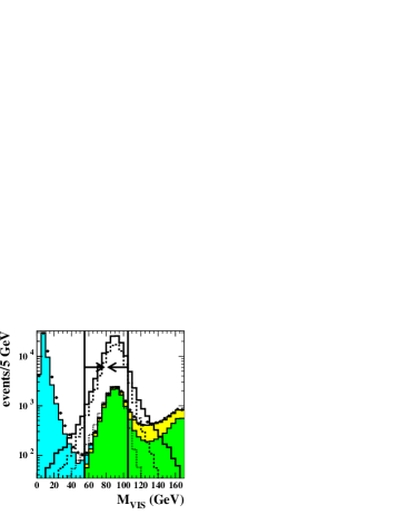
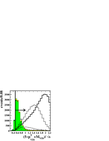
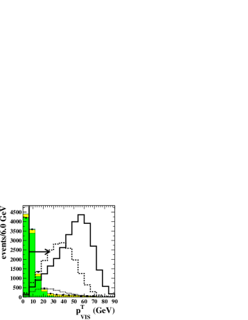
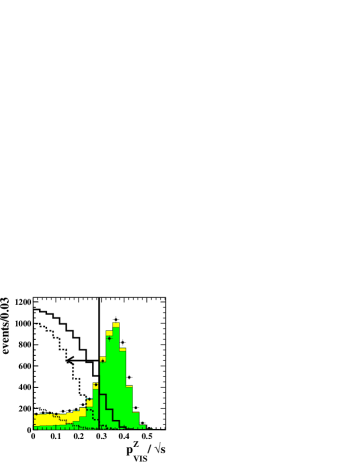
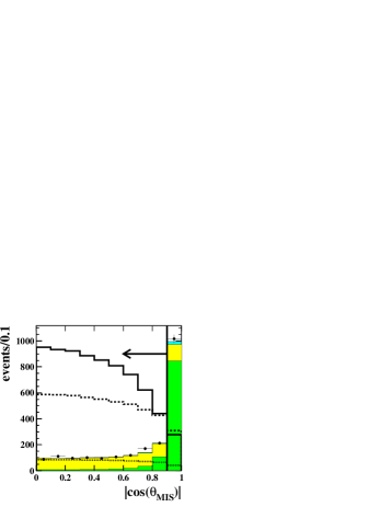
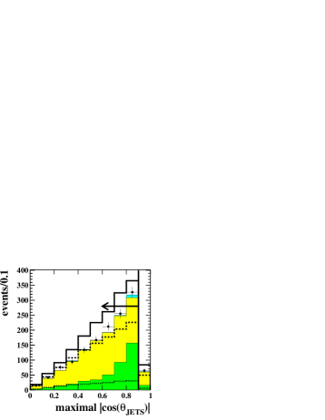
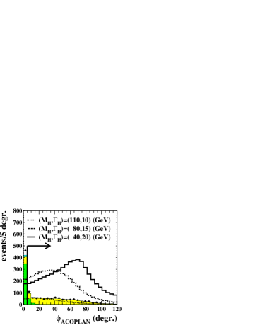
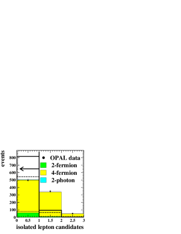
Figure 1: Distribution of the preselection variables after the preselection cuts (1)-(5). All classes of Standard Model background and data are added for all analysed centre-of-mass energies. The distributions of three arbitrarily scaled signal hypotheses at $\sqrt{s}=206$ GeV are displayed as open histograms.

For each individual centre-of-mass energy there is good agreement between the numbers of expected background events and observed candidates after the preselection. Table 2 gives the number of preselected events summed over all centre-of-mass energies. Figure 1 shows the distributions for background classes summed over all centre-of-mass energies and three arbitrarily scaled signal distributions (at a centre-of-mass energy of 206 GeV). The efficiencies of the preselection vary on average between 39 % and 55 % for small decay widths and between 45 % and 53 % for larger decay widths above $\Gamma_{\mathrm{H}}$ = 100 GeV.

4.3 Likelihood analysis

To consider the changing kinematic properties of the signal hypotheses in an optimal way, five different likelihood-based analyses for the signal and background discrimination were applied after the preselection. By a likelihood analysis we denote the combination of a set of likelihood input variables, a so-called likelihood, and the corresponding reference distributions of these variables. The reference distributions are filled with events of the specific classes for which the likelihood is calculated. The classes considered in this search are the two- and four-fermion backgrounds and the signal events. The two-photon events are negligible after the preselection. The search uses combinations of two likelihoods and three fixed signal mass ranges for unweighted reference histograms.

To compare the kinematic properties of a selected data event to the hypothesis ($M_{\mathrm{H}}$,$\Gamma_{\mathrm{H}}$) when evaluating the likelihood, one in principle has to fill weighted signal reference distributions for each hypothesis ($M_{\mathrm{H}}$,$\Gamma_{\mathrm{H}}$). This will soon lead to an unmanageable technical effort, given the number of hypotheses scanned. Therefore a compromise was sought in which certain kinematic properties of the signal were emphasised and simultaneously the number of reference histograms kept small. This was achieved by filling unweighted signal reference histograms. For most of the ($M_{\mathrm{H}}$,$\Gamma_{\mathrm{H}}$) hypotheses all signal masses were used for filling the reference histograms. This reflects the fact that for a very large decay width of the Higgs boson the possible values of kinematical variables are also smeared out over a large range. It was, however, found that the sensitivity of the likelihood selection (i.e. the median expected upper limits on $\sigma(M_{\mathrm{H}},\Gamma_{\mathrm{H}})\times\mathrm{BR}(\mathrm{H}\to E_{\mathrm{MIS}})$) could be increased further for small widths below 50 GeV by filling reference histograms with signal masses from 50-80 GeV and from 80-120 GeV for intermediate and heavy Higgs boson masses respectively.  A first likelihood was designed for a signal consisting of small masses ($M_{\mathrm{H}}$ < 80 GeV) or large masses and a very large width ($\Gamma_{\mathrm{H}}$ $\geq 110$ GeV). In this likelihood input variables are used exploiting the characteristics of the dominant fraction of light masses in the signal mass distribution. However for signal masses above $M_{\mathrm{H}}$ = 80 GeV and small or moderate (i.e. below 110 GeV) decay widths, the contribution of large masses dominates the signal mass distribution. In this case the kinematics and topology of the signal events are determined by the higher masses close to the kinematic limit. A second likelihood is therefore built with input variables optimised for such signal characteristics. In the following the choice of the inputs for the two optimised likelihoods are presented.

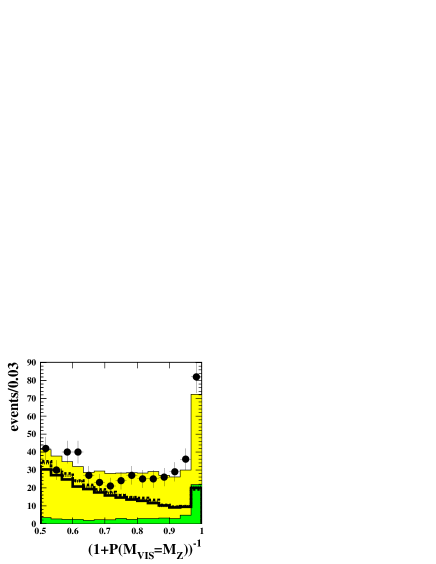
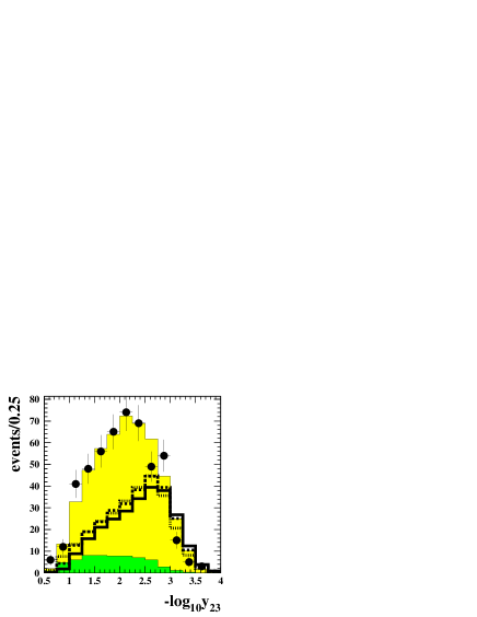
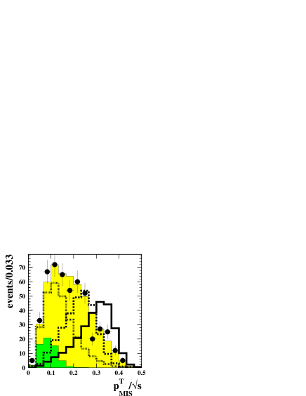
Figure 3: Distributions of the likelihood variables. All classes of Standard Model background and data are added for all centre-of-mass energies analysed. The distributions of three arbitrary scaled signal examples at $\sqrt{s}=206\,\mbox{GeV}$ are displayed as open histograms. The variables shown contribute to likelihood 1 and 2 as they exploit general properties of the signal signature.

The first three input variables are used in both likelihoods (see Figure 3) .

• $(1+{\cal P}(M_{\mathrm{VIS}}\equiv\mathrm{M_{Z}}))^{-1}$
  ${\cal P}(M_{\mathrm{VIS}}\equiv\mathrm{M_{Z}})$ is the probability of a kinematical $\chi^{\mathrm{2}}$ fit of the jet four-vectors under the assumption that the invariant mass of the two jets is compatible with the Z boson mass. This variable depends only weakly on the Higgs mass. For events with non-converging fit the probability is set to zero. They therefore accumulate at a value of 1.

• $-\log y_{32}$
  The Durham algorithm groups two energy flow objects $i$ and $j$ into a jet as long as their separation in phase space $y_{ij}=2\times min(E^{2}_{i},E^{2}_{j})\times(1-\cos(\theta_{ij})/E^{2}_{\mathrm{VIS}}$ is smaller then the cut value $y_{\mathrm{cut}}$. The number of jets in a event is predefined to be 2, $y_{32}$ is the value of $y_{\mathrm{cut}}$ where the two-jet topology of the event changes to a three-jet topology. Hence the negative logarithm of the so-called jet resolution parameter $y_{32}$ is a measure for the jet topology being more two-jet like (large value of $-\log y_{32}$) or three-jet like (small value of $-\log y_{32}$).

• $p^{T}_{\mathrm{MIS}}/\sqrt{s}$
  The transverse missing momentum $p^{T}_{\mathrm{MIS}}$ is one of the most prominent characteristics of signal-like events, but depends very much on the Higgs boson mass. For a heavy Higgs boson produced close to the kinematic threshold almost at rest, the Z boson has almost no boost and decays into two more or less back-to-back jets. In this case the discriminating power of the variable is lost.

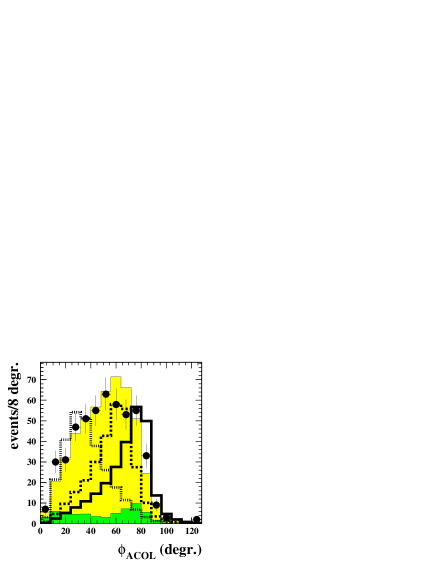
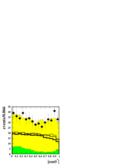
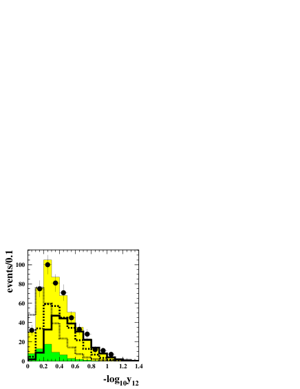
Figure 4: Distributions of the likelihood variables. All classes of Standard Model background and data are added for all centre-of-mass energies analysed. The distributions of three arbitrary scaled signal examples at $\sqrt{s}=206\,\mbox{GeV}$ are displayed as open histograms. The variables shown are combined with the ones of Figure 3 to construct the likelihood 1 used in a general search at different $M_{\mathrm{H}}$ and $\Gamma_{\mathrm{H}}$.

The next three variables (see Figure 4) complete the first likelihood, which is used for all Higgs masses in the domain of very large width > 110 GeV or low Higgs masses < 80 GeV.

• $\phi_{\mathrm{ACOL}}$
  The acolinearity angle $\phi_{\mathrm{ACOL}}$ of the two-jet system is obtained by subtracting the three-dimensional angle between the reconstructed jet-axes from $180^{\circ}$. Events containing a low-mass Higgs boson exhibit on average a larger acolinearity than the background.

• $|\cos\theta^{\ast}|$
  The Gottfried-Jackson angle $\theta^{\ast}$, is defined as the angle between the flight direction of the Z boson in the laboratory frame and the direction of the decay products of the Z boson boosted into the Z boson rest-frame. The variable tends to have smaller values for the signal.

• $-\log y_{21}$
  The variable $-\log y_{21}$ is analogous to $-\log y_{32}$ and measures the compatibility of the event with a two-jet topology. Two-jet events tend to accumulate at small values of $-\log y_{21}$.
  

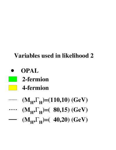
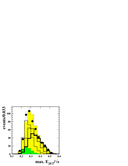
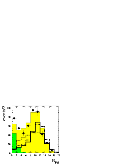
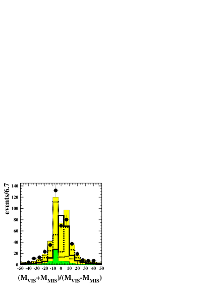
Figure 5: Distributions of the likelihood variables. All classes of Standard Model background and data are added for all centre-of-mass energies analysed. The distributions of three arbitrary scaled signal examples at $\sqrt{s}=206\,\mbox{GeV}$ are displayed as open histograms. The variables shown have a larger discrimination power for a heavier Higgs boson and contribute with the variables of Figure 3 to the second likelihood.

The last three variables (see Figure 5) tune the second likelihood to become more sensitive for large Higgs boson masses and small to moderate widths.

• $E^{\mathrm{Max}}_{\mathrm{JET}}/\sqrt{s}$
  The variable $E^{\mathrm{Max}}_{\mathrm{JET}}$ measures the energy of the most energetic of the two jets. This is on average higher for the four-fermion background, due to the boost of the W and Z pairs, whereas heavy Higgs bosons and a Z boson are produced at rest.

• $R_{P_{ti}}$
  This variable is the significance of the acoplanarity between the two jets, taking into account detector resolution and acceptance. The discrimination power is enhanced by weighting the acoplanarity with the average jet polar angle, since transverse jet directions are more precisely measured at large polar angles. Signal events tend to have a more significant acoplanarity and thus larger values of $R_{P_{ti}}$ than background. The precise definition of $R_{P_{ti}}$ can be found in the OPAL analyses of $\mathrm{ZZ\rightarrow q{\overline{q}}\nu{\overline{\nu}}}$ events [25].

• $(M_{\mathrm{VIS}}+M_{\mathrm{MIS}})/(M_{\mathrm{VIS}}-M_{\mathrm{MIS}})$
  This variable, described in [26], uses two strongly correlated quantities, the invariant missing mass $M_{\mathrm{MIS}}$ and the visible mass of the event $M_{\mathrm{VIS}}$. Depending on the mass reconstruction accuracy it can have positive or negative values. The signal distribution of this variable is broader and accumulates at higher values than for the two- and four-fermion events, which are distributed more narrowly around the origin.

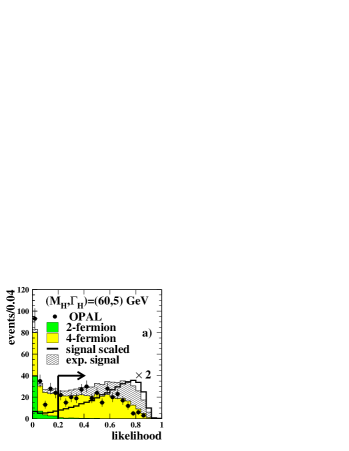
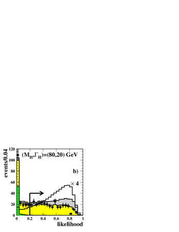
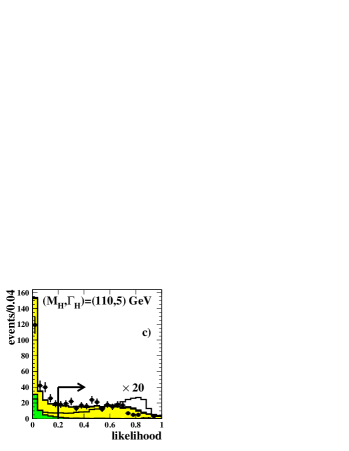
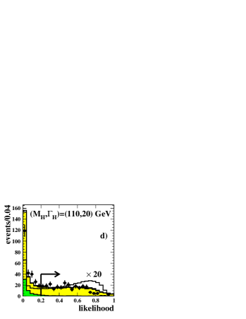
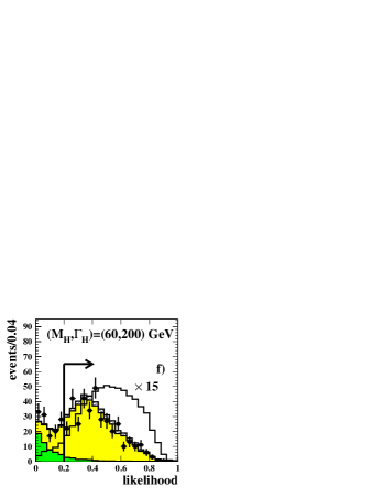
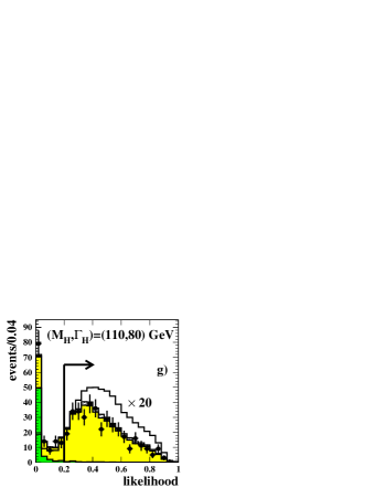
Figure 6: Examples of some of the likelihood selections. Figure 6 e), f), h) corresponds to analysis A1 (as labelled in Table 3 and 6), a) to A3, b) to A4 and c), d) to A5. The OPAL data and the expected 2-fermion and 4-fermion background are added for all analysed centre-of-mass energies. The signal hypothesis in the hatched histograms is normalised to the number of expected signal events and added to the background. The open histograms display the shapes of scaled signal distributions.

From the two likelihoods and three ranges of signal masses filled in the reference histograms one has six analyses to search for the different hypotheses in $M_{\mathrm{H}}$ and $\Gamma_{\mathrm{H}}$. The study of the median expected $\sigma(M_{\mathrm{H}},\Gamma_{\mathrm{H}})\times\mathrm{BR}(\mathrm{H}\to E_{\mathrm{MIS}})$ shows that five of these six are sufficient to have an optimally efficient analysis for each signal hypothesis characterised by $M_{\mathrm{H}}$ and $\Gamma_{\mathrm{H}}$ (see Figure 2) in the range studied. Likelihood 1 was not used with the reference distribution filled for the signal mass range of 80 to 120 GeV. Figure 6 a) to c) and g) to h) display examples for the likelihood distributions of all five analyses used. In the histograms the events selected at all five centre-of-mass energies are added up, although each centre-of-mass energy was evaluated separately in the limit setting as explained in Section 5.1. The appropriate likelihood was calculated for each background, data and signal event. In case of a signal event it was added to the histogram with the weight defined in Equation 7. The number of expected signal events is normalised according to Equation 6. The use of different analyses gives rise to varying shapes of the likelihood distributions of the background. Also the various shapes of the signal likelihood distributions are visible for different $M_{\mathrm{H}}$ and $\Gamma_{\mathrm{H}}$. Since the form of the likelihood distributions for signal and background can yield additional information in the limit calculation, only a loose cut is applied in the likelihood selection, requiring a signal likelihood larger than 0.2.

4.4 Correction of background and signal efficiencies

A correction is applied to the number of expected background events and the signal efficiencies due to noise in the detectors in the forward region which is not modelled by the Monte Carlo. The forward energy veto used in the preselection can accidentally be triggered by machine backgrounds. The correction factor is derived from the study of random beam crossings, and applied individually for each year of data taking. Random beam crossing events were recorded when no physics trigger was active. The fraction of events that fail the veto on activity in the forward region is below 3.4 % for all runs analysed. The detailed breakdown of the fraction of accidentally vetoed events is given in the last column of Table 1.

4.5 Systematic uncertainties

A possible signal in the data would reveal itself by altering the shapes of the distributions of the discriminating variables. Thus a systematic deviation in the description of a reconstructed observable between Standard Model Monte Carlo and a data sample in which the signal is absent, could wrongly be attributed to the presence of a signal.

The systematic uncertainties in the Monte Carlo description of the kinematic event variables are studied in two control samples at a centre-of-mass energy of 206 GeV. In the first control sample, called two-fermion control-sample in the following, radiative returns contributing to the $\mbox{$\mathrm{q}\bar{\mathrm{q}}$}(\gamma)$ processes with photons detected at large angles are selected and the tagged ISR photon is removed from the event in Monte Carlo and data. This creates a $\mathrm{q}\bar{\mathrm{q}}$-like topology with missing momentum at large angles. The second control sample, called four-fermion control-sample, is obtained by selecting $\mbox{$\mathrm{W}^{+}\mathrm{W}^{-}$}\to\mbox{$\mathrm{q}\bar{\mathrm{q}}$}l\nu$ events and removing the identified isolated lepton from the events in Monte Carlo and data. After this procedure control samples possess a topology very similar to signal events. For all kinematic variables $x$ of the preselection and the likelihood selection the mean $\overline{x}$ and the width of the distribution ($RMS$) are compared between Monte Carlo and data, for the two-fermion and four-fermion control-samples. The observables in the two-fermion and four-fermion Monte Carlo are then modified separately according to $x^{\mathrm{NEW}}_{\mathrm{MC}}=(x^{\mathrm{OLD}}_{\mathrm{MC}}-{\overline{x}}_{\mathrm{MC}})\times\frac{RMS_{\mathrm{DATA}}}{RMS_{\mathrm{MC}}}+{\overline{x}}_{\mathrm{DATA}}$. Then all five likelihood selections are repeated separately and the relative change in the number of selected events compared to the unmodified case is taken as the systematic uncertainty.

Since the analysis labelled A1 in Table 3 is used over a large range of the search plane (see Figure 2), the systematic uncertainties on the background determined in this analysis A1 are taken as an estimate for the background for all analyses. To determine the effect of the systematic uncertainty on the signal efficiencies, one has to take into account the fact that the kinematic properties of the signal depend on the assumed Higgs mass and decay width. Twelve representative hypotheses are studied with $M_{\mathrm{H}}$ chosen to be 20, 60 or 110 GeV and $\Gamma_{\mathrm{H}}$ taking values of 5, 20, 70 and 200 GeV. For these hypotheses the signal Monte Carlo is modified according to the four-fermion correction factors, representing the dominant remaining background after the cut on the signal likelihood. The relative change in selected event weights compared to the unmodified case is then taken as an estimate of the systematic uncertainty on the signal efficiency for a given hypothesis. The root-mean-square of all twelve hypotheses is applied as an ($M_{\mathrm{H}}$,$\Gamma_{\mathrm{H}}$)-independent estimate for the whole search area and for all centre-of-mass energies (see Table 4).

The W pairs are very effectively reduced in the preselection by the isolated lepton veto. Due to the importance of this veto the uncertainty from the lepton isolation angle and the vetoed cone energy is studied in the following way. The half-cone angle of the outer cone is increased and decreased by two degrees, following the studies in [27], and the relative effect on the selection determined. Furthermore the cone energy is varied by 7.4 % and the analyses are repeated. The value of the cone energy rescaling is determined by the relative deviation of the mean of the measured energy of the lepton candidates in the inner cone between data and Monte Carlo in the $\mbox{$\mathrm{W}^{+}\mathrm{W}^{-}$}\to\mbox{$\mathrm{q}\bar{\mathrm{q}}$}l\nu$ sample. For signal efficiencies an analogous study was performed at the twelve points described above.  Both results for the relative change of the selection for the cone opening half-angle and cone energy variation are added in quadrature and the root-mean-square of the 12 ($M_{\mathrm{H}}$,$\Gamma_{\mathrm{H}}$) hypotheses was taken to yield the total uncertainty associated with the isolated lepton veto (see Table 4).

The theoretical prediction on the cross-section for the two- and four-fermion processes adds an uncertainty of 2 % to the background uncertainty [28]. Finally, the uncertainty due to the limited Monte Carlo statistics is evaluated.

Table 5 summarises the results of the studies. All uncertainties are assumed to be uncorrelated and the individual contributions are added in quadrature to obtain the total systematic uncertainties on the background expectation and signal efficiency. The dominant systematic uncertainties on the signal efficiency arise from the description of the kinematic variables. The background expectation is more affected by the uncertainty in the isolated lepton veto, as the main contribution of the background stems from four-fermion processes. But the uncertainty associated with the description of the kinematic variables is of similar magnitude. The limits quoted in Section 5.1 were calculated including the uncertainties of Table 5. To estimate the extent to which the limits depend on the size of the systematic uncertainties, the limit calculation was repeated doubling the systematic uncertainties. A comparison of the limits with single and double systematic uncertainties, done at similar representative points as used for the systematic studies, showed that the excluded cross-sections typically decrease between a half and one and a half percent. A maximal reduction of 2.1 % was found.

5 Results

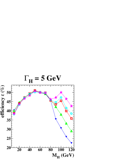
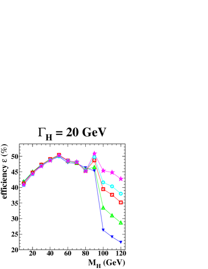
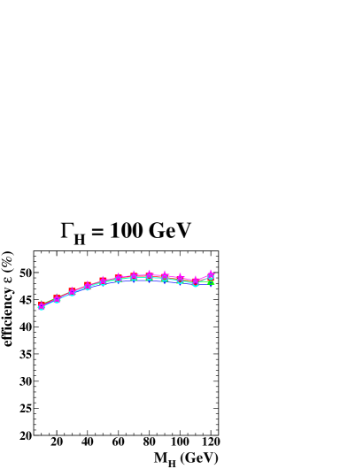
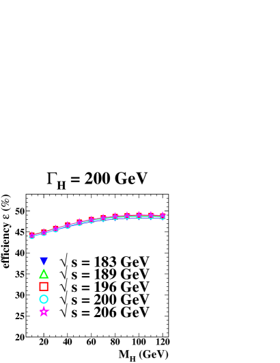
Figure 7: Examples for the selection efficiency after a cut on the signal likelihood greater than 0.2 versus the Higgs mass $M_{\mathrm{H}}$ as function of the assumed decay width $\Gamma_{\mathrm{H}}$ at the different $\sqrt{s}$. The error is the binomial error on the selected event weights and smaller than the markers. Lines are added to guide the eye.For a large $\Gamma_{\mathrm{H}}$ signal hypothesis, the kinematic distributions of events and the distribution of weights assigned to this events are broader. Therefore it is more likely to select a larger fraction of the event weights leading to a higher and more uniform efficiency. For a smaller widths $\Gamma_{\mathrm{H}}$ the efficiency to detect relatively heavy and a more Standard Model like Higgs boson is more restricted by the available $\sqrt{s}$.

The results of the search using each of the five different likelihood selections, labelled A1-A5, after a cut on the likelihood larger than 0.2 are summarised in Table 6, which compares the numbers of observed candidates with the Standard Model background expectations. The data are compatible with the Standard Model background expectations. The remaining four-fermion background consists predominantly of W pairs, representing roughly three quarters of the background at energies above the Z pair threshold. Figure 7 shows examples for signal efficiencies. For small decay widths the dependence on the centre-of-mass energy is weak up to $M_{\mathrm{H}}$ $\approx$ 80 GeV, and for large widths it is weak up to the kinematic limit. Because of the centre-of-mass energy dependence of the Bjorken cross-section of a Higgs boson with mass $M_{\mathrm{H}}$, the lower centre-of-mass energies contribute more significantly to the sensitivity for lighter Higgs bosons (see e.g. in [8]). For very light Higgs bosons the efficiency is moderately reduced by the preselection cuts demanding a sizeable amount of missing energy. In the case of broader Higgs resonances with high mass, one observes a generally enhanced efficiency since the chance of selecting events from the low mass tail compensates the suppression due to the falling production cross-section of a heavy Higgs boson.

5.1 The upper limits on the production cross-section times branching ratio

As no significant excess over the expected background is observed in the data, upper limits are calculated on the model-independent cross-section $\sigma(M_{\mathrm{H}},\Gamma_{\mathrm{H}})\times\mathrm{BR}(\mathrm{H}\to E_{\mathrm{MIS}})$ scaled to $\sqrt{s}=206$ GeV.  As the likelihood distributions are only loosely cut, one can use not only the information from the integral number of selected events (Table 6) but also from the shape in a likelihood ratio [29] to set more sensitive upper limits. For each centre-of-mass energy separately, each bin with a signal likelihood larger than 0.2 in the distributions of expected signal, background and selected data is treated as a search channel. For each centre-of-mass energy the number of expected signal events is scaled to the total cross-section (Equation 6). As with the analysis described in [30], the likelihood distributions are given as discriminating input to a limit program [31]. A likelihood ratio is used to determine the signal confidence level, $\mathrm{CL_{S}}$, defined in [29, 31], which excludes the presence of a possible signal according to the modified frequentist approach [31]. Additionally the program calculates the median upper number of signal events that could be excluded at 95 % confidence level (CL). This number is then scaled to the total cross-section at the centre-of-mass energy of 206 GeV for each ($M_{\mathrm{H}}$,$\Gamma_{\mathrm{H}}$) hypothesis. The systematic uncertainties on the background expectations and signal selection efficiencies are included according a generalisation of the method described in [32].

A very fine scan of the ($M_{\mathrm{H}}$,$\Gamma_{\mathrm{H}}$)-plane was performed by simulating the spectra of Higgs bosons with a mass $M_{\mathrm{H}}$ from 1 to 120 GeV and widths $\Gamma_{\mathrm{H}}$ starting at 1 GeV up to 3  TeV. The Higgs boson mass was simulated in steps of $\delta M_{\mathrm{H}}=1$ GeV. Simulated values of $\Gamma_{\mathrm{H}}$ are spaced in steps of 1 GeV up to 5 GeV. A spacing of $\delta\Gamma_{\mathrm{H}}=5$ GeV is chosen from $\Gamma_{\mathrm{H}}$ = 5 GeV to $\Gamma_{\mathrm{H}}$ = 750 GeV. Above this value steps of $\delta\Gamma_{\mathrm{H}}=50$ GeV are adopted up to the maximal $\Gamma_{\mathrm{H}}$ of 3 TeV.

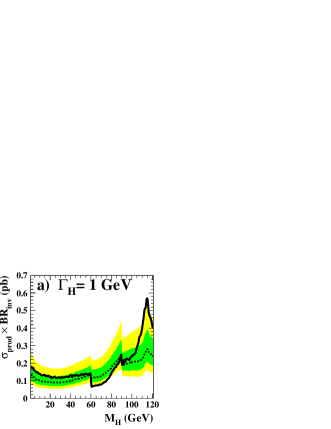
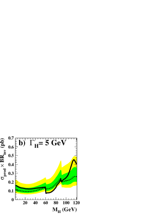
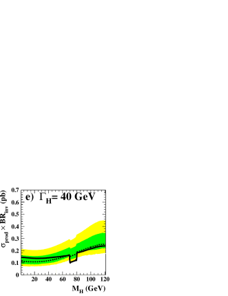
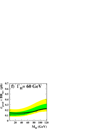
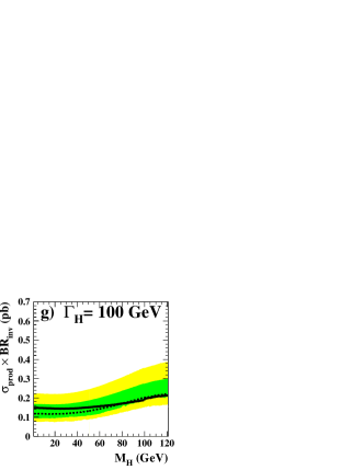
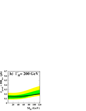
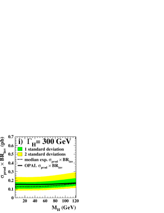
Figure 8: The model independent upper limits at 95 % CL on the production cross-section times branching ratio, $\sigma_{\mathrm{prod}}\times BR_{\mathrm{inv}}$, scaled to a centre-of-mass energy of 206 GeV for Higgs mass $M_{\mathrm{H}}$ and some examples of the Higgs decay width $\Gamma_{\mathrm{H}}$. The discontinuities in the limits reflect the changes in the analysis used at this mass (see Figure 2).

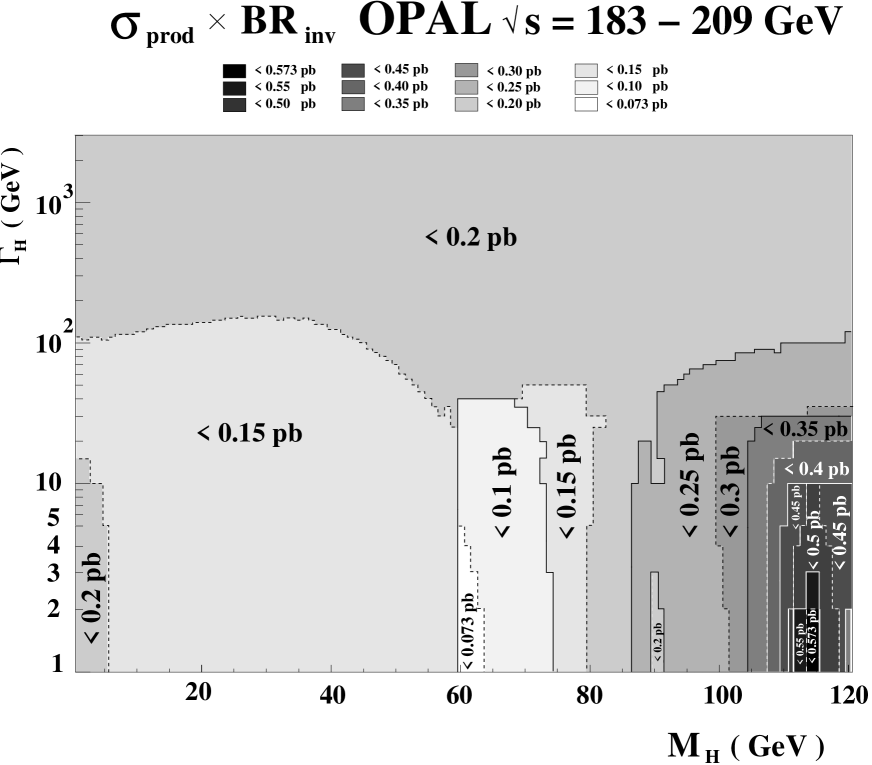
Figure 9: The exclusion contours at 95 % CL on the model independent production cross-section times branching ratio, $\sigma_{\mathrm{prod}}\times BR_{\mathrm{inv}}$, for Higgs boson mass $M_{\mathrm{H}}$ and the Higgs boson decay width $\Gamma_{\mathrm{H}}$ up to 3 TeV (note a change in logarithmic scale below $\Gamma_{\mathrm{H}}$ = 5 GeV for better visibility). Solid and dashed lines delimit areas of excluded upper limits. Cross-sections times branching ratio between 0.07 pb and 0.57 pb are excluded with the OPAL data above $\sqrt{s}=183$ GeV.

Examples of the projections of the observed upper cross-section limits together with the median expected upper limits and the corresponding one and two standard deviation bands on the expected limits are displayed in Figure 8 for some choices of $\Gamma_{\mathrm{H}}$. Above a width of 300 GeV the exclusion plots look quite similar to the example displayed in Figure 8i) because the excluded limits do not change very much. The observed limits for $\Gamma_{\mathrm{H}}$ $\gtrsim$ 60 GeV are well contained in the one standard deviation bands on the expectations and generally do not exceed two standard deviations except in Figure 8 a) at $M_{\mathrm{H}}$ = 114 GeV.  The discontinuities in the graphs correspond to changes in the analyses. As one can observe, below $\Gamma_{\mathrm{H}}$ $\lesssim 40$ GeV the analysis are changed more often. Therefore the chance is higher that in a few bins there are statistical fluctuations in the selected data, that lead to a deviation of more than one standard deviation around the median. Also the data selected are highly correlated, as one can see for example in the upward fluctuation around $M_{\mathrm{H}}$ = 114  GeV visible in Figure 8 a)-c). All results for the observed upper limits on $\sigma(M_{\mathrm{H}},\Gamma_{\mathrm{H}})\times\mathrm{BR}(\mathrm{H}\to E_{\mathrm{MIS}})$ are summarised in a contour plot (Figure  9) in the scanned ($M_{\mathrm{H}}$,$\Gamma_{\mathrm{H}}$)-plane. Above $\Gamma_{\mathrm{H}}$ = 200 GeV the observed upper limits are in the range of 0.15 pb to 0.18 pb for all $M_{\mathrm{H}}$ and vary very little. For such large $\Gamma_{\mathrm{H}}$ the recoil mass distribution of the Higgs tends to be more and more uniformly stretched out over the mass range explored. There is not much difference in the selection of signal events for a Higgs boson with e.g. a width of 400 GeV or 600 GeV in the considered range of Higgs masses. This prevents any specific discriminating kinematical properties from being assigned to the expected signal as signal masses of a broad kinematical range are selected with roughly equal probability. Therefore only one likelihood analysis is used in this part of the search area, selecting the same subset of data and background. Since the upper limit on the model-independent cross-section refers to a production cross-section at a centre-of-mass energy of 206 GeV, it must become independent of ($M_{\mathrm{H}}$,$\Gamma_{\mathrm{H}}$) for an extremely large $\Gamma_{\mathrm{H}}$. In this case the shape of the Higgs signal would just be a box, weighted with the production cross-section from 1 GeV to the kinematic limit of about 115 GeV. The data are then compared to an approximately constant signal expectation. Hence the upper limit on the cross-section is approximately independent of the ($M_{\mathrm{H}}$,$\Gamma_{\mathrm{H}}$) hypothesis at a value of roughly 0.16 pb. For resonances with a decay width smaller than 200 GeV there are regions where the limits are below 0.15 pb or even 0.1 pb for $M_{\mathrm{H}}$ between 60 and 74 GeV. In this mass range the number of data events selected is smaller than expected. Above $M_{\mathrm{H}}$ of 85 GeV the upper limits become larger than 0.2 pb and rise considerably for small widths below 40 GeV (see Figure 8 a-e). This is due to the fact that the Higgs mass approaches the kinematic limit and the likelihoods which rely on kinematical variables like $p^{\mathrm{T}}_{\mathrm{MIS}}$ lose discrimination power. A maximal value of 0.57 pb is observed for $M_{\mathrm{H}}$ of 114 GeV and $\Gamma_{\mathrm{H}}$ of 1 GeV corresponding to a circa two-$\sigma$ excess in the data.

It should be kept in mind that no optimisation of the search has been performed for $\Gamma_{\mathrm{H}}$ below 5 GeV. In the region of heavy Higgs boson mass $\gtrsim$ 105 GeV and small width a search using recoil mass spectra would be more sensitive. Therefore this region is more sensitively covered by searches that have been performed by the LEP experiments documented in [2].

5.2 Interpretation of the result in the stealthy Higgs scenario

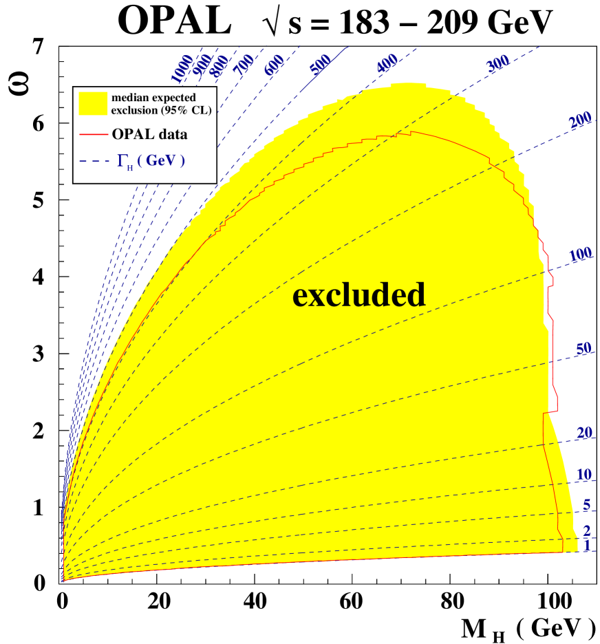
Figure 10: The exclusion contours at 95 % CL on the Higgs mass $M_{\mathrm{H}}$ and the Higgs-phion coupling $\omega$ of the stealthy Higgs model. The values of $\omega$ are related to the decay width $\Gamma_{\mathrm{H}}$ via $\Gamma_{\mathrm{H}}(M_{\mathrm{H}})=\Gamma_{\mathrm{SM}}(M_{\mathrm{H}})+\frac{\omega^{2}v^{2}}{32\,\pi\,M_{\mathrm{H}}}$, in the case of massless phions (see Equation 5). Contours of fixed $\Gamma_{\mathrm{H}}$ are also shown in the plot as dashed lines.

Interpreting the width $\Gamma_{\mathrm{H}}$ of a Higgs boson according to Equation 5, and setting $m_{\mathrm{phion}}$ to zero, it was possible to set limits on $\omega$ in the stealthy Higgs scenario. A range from $\omega=0.04$ to $\omega=24.45$ was probed. The excluded regions are shown in Figure 10 at 95 % confidence level (CL) in the $\omega$-$M_{\mathrm{H}}$ parameter space. To illustrate the Higgs boson width according to Equation 5, contours of fixed $\Gamma_{\mathrm{H}}$ corresponding to a given mass $M_{\mathrm{H}}$ and coupling $\omega$ are added to the plot.  The maximum excluded invisible width is about $\Gamma_{\mathrm{H}}$ = 400 GeV for Higgs boson masses $\lesssim$ 35 GeV, decreasing slowly to $\Gamma_{\mathrm{H}}$ = 115 GeV for $M_{\mathrm{H}}$ = 100 GeV. The minimal exclusion of $\omega=0.04$ is observed at $M_{\mathrm{H}}$ = 1 GeV and the maximal exclusion is $\omega=5.9$ for $M_{\mathrm{H}}$ = 73 GeV.  For $\omega$ between 0.04 and 0.59 a Higgs mass from 1 to 103 GeV could be excluded. The maximal excluded Higgs mass was 103 GeV for width between 1 and 3 GeV, compared with the expected exclusion of 106 GeV.

The results presented in this study extend the previous decay-mode independent searches for new scalar bosons with the OPAL detector [5] to regions of larger couplings and higher Higgs boson masses. In [5] an interpretation within the stealthy Higgs model yielded a maximal excluded coupling $\omega$ for masses around 30 GeV, where $\omega$ was excluded up to $\omega=2.7$. That study excluded Higgs boson masses up to $M_{\mathrm{H}}$ = 81 GeV. It should be pointed out that the decay-mode independent searches also studied Higgs widths between 0.1 and 1 GeV and therefore cover the gap between searches within scenarios assuming a narrow decay width of the invisibly decaying Higgs boson [2] and the search presented in this paper up to $M_{\mathrm{H}}$ = 81 GeV.

6 Conclusions

A dedicated search was performed in the channel $\mathrm{e}^{+}\mathrm{e}^{-}\to\mathrm{H}\mathrm{Z}$ with $\mathrm{Z}\to\mbox{$\mathrm{q}\bar{\mathrm{q}}$}$ and the non-Standard Model decay $\mathrm{H}\to E_{\mathrm{MIS}}$ final state allowing for invisible decay widths of the Higgs boson from 1 GeV up to 3 TeV. The data taken by the OPAL detector at LEP above the W pair threshold were analysed. No indication for a signal was found and upper limits were set on $\sigma(M_{\mathrm{H}},\Gamma_{\mathrm{H}})\times\mathrm{BR}(\mathrm{H}\to E_{\mathrm{MIS}})$. The maximal upper limit is 0.57 pb at $M_{\mathrm{H}}$ = 114 GeV and $\Gamma_{\mathrm{H}}$ = 1 GeV. Over the scanned region of the ($M_{\mathrm{H}}$,$\Gamma_{\mathrm{H}}$)-plane upper limits are generally of the order of 0.15 pb, especially for large values of $\Gamma_{\mathrm{H}}$ $\gtrsim$ 400 GeV or Higgs boson masses $\lesssim$ 85 GeV.

The limits were interpreted in the stealthy Higgs scenario assuming the presence of a large number of massless singlet states. Limits were calculated on the coupling $\omega$ to a hidden scalar sector of the Higgs boson with a given mass $M_{\mathrm{H}}$. A large part of the parameter plane kinematically accessible with LEP  2 was excluded extending a previous exclusion published in [5]. Values for $\omega$ between 0.04 ($M_{\mathrm{H}}$ = 1 GeV) and 5.9 ($M_{\mathrm{H}}$ = 73 GeV) were excluded, and for certain values of $\omega$ Higgs boson masses are excluded up to $M_{\mathrm{H}}$ = 103 GeV. The possible non-detection of a light Higgs boson at the LEP searches due to non-Standard Model invisible Higgs boson decays is therefore restricted to the case of extremely large decay widths $\gtrsim$ 400 GeV.

binned $\sqrt{s}$       nominal $\sqrt{s}$ (GeV)		year	int. luminosity (pb-1)	accid. veto (%)
$>$ 180–186	183	1997	40.0	3.37
$>$ 186–193	189	1998	199.8	2.24
$>$ 193–198	196	1999	70.4	2.53
$>$ 198–203	200	1999	112.0	2.96
$>$ 203–209	206	2000	206.9	2.22

Table 1: Breakdown of the analysed integrated data luminosities according to the centre-of-mass energies. The data was binned in five nominal centre-of-mass energies. The last column states the reduction of the signal efficiencies and expected background rates due to accidental triggering of the forward energy veto in the preselection, which is not modelled in the Monte Carlo.

cut	$\gamma\gamma$	qq( $\gamma$)	4-fermion	total SM	data
(1)-(5)	48795	15639	4880	69314	74178
(6)	148	10359	1394	11901	11779
(7)	62	9128	1336	10526	10472
(8)	44	4897	1167	6108	6264
(9)	33	1061	964	2058	2116
(10)	18	425	895	1338	1387
(11)	18	423	879	1320	1368
(12)	4	68	820	892	899
(13)	4	60	441	505	498

Table 2: Expected number of Standard Model background events after the preselection normalised to a data luminosity of 629.1 $\mathrm{pb^{-1}}$. The total SM background after preselection is expected to be 505 $\pm$ 5(stat) $\pm$ 21(syst). The contributions of the different subclasses are broken down in column two to four for the two-photon, two-fermion and four-fermion processes respectively.

analysis	background uncertainty
label    likelihood     reference mass range (GeV)	kinematic var.  isol. lepton veto
A1             1          1–120	2.4 %	2.4 %
A2             2          1–120	1.6 %	2.3 %
A3             1          50–80	1.0 %	2.5 %
A4             2          50–80	1.6 %	2.6 %
A5             2         80–120	1.1 %	1.5 %
choice for uncertainty	2.4 %	2.4 %

Table 3: Results of the study of systematic uncertainties of the expected background for the five kinds of analyses, labelled A1-A5, used in the search (see Figure 2) at a centre-of-mass energy of 206 GeV. Since the analysis labelled A1 covers the largest part of the search area, its uncertainty was chosen as representative uncertainty on the background due to the uncertainty in the kinematic variables and the isolated lepton veto at all centre-of-mass energies.

signal hypothesis	efficiency uncertainty
$M_{\mathrm{H}}$ (GeV)  $\Gamma_{\mathrm{H}}$ (GeV)	kinematic var.  isol. lepton veto
20         5	0.6 %	0.6 %
20       20	0.4 %	0.7 %
20       70	0.3 %	0.7 %
20     200	0.1 %	0.7 %
60         5	0.7 %	0.8 %
60       20	0.7 %	0.8 %
60       70	0.2 %	0.8 %
60     200	0.3 %	0.7 %
110         5	5.5 %	0.7 %
110       20	2.9 %	0.8 %
110       70	1.3 %	0.8 %
110     200	0.1 %	0.8 %
all $M_{\mathrm{H}}$ and $\Gamma_{\mathrm{H}}$	1.9 %	0.7 %

Table 4: Results of the study of systematic uncertainties in twelve representative ($M_{\mathrm{H}}$,$\Gamma_{\mathrm{H}}$)-points at a centre-of-mass energy of 206 GeV. For each source the root-mean-square of the individual uncertainties in the twelve points was taken to get an ($M_{\mathrm{H}}$,$\Gamma_{\mathrm{H}}$) independent estimate of the uncertainty at all centre-of-mass energies.

source	background uncertainty	efficiency uncertainty
kinematic variables	2.4 %	1.9 %
isolated lepton veto	2.4 %	0.7 %
limited MC statistics	1.0 %	0.2 %
prediction 2- and 4-f cross-sect.	2.0 %	-
total uncertainty	4.1 %	2.0 %

Table 5: Results of the study of systematic uncertainties of the background for the five analyses (see Table 3) and of the signal efficiencies in twelve representative ($M_{\mathrm{H}}$,$\Gamma_{\mathrm{H}}$)-points (see Table 4) at a centre-of-mass energy of 206 GeV. The total uncertainty on background expectation and signal efficiency is applied at all centre-of-mass energies and for all ($M_{\mathrm{H}}$,$\Gamma_{\mathrm{H}}$) hypotheses.

label   reference masses	likelihood	2-fermion	4-fermion	total SM	data
A1                1–120 GeV	type 1	11	374	385 $\pm$ 4 $\pm$ 16	369
A2                1–120 GeV	type 2	3	378	381 $\pm$ 4 $\pm$ 16	370
A3                50–80 GeV	type 1	5	315	320 $\pm$ 3 $\pm$ 13	305
A4                50–80 GeV	type 2	2	315	317 $\pm$ 3 $\pm$ 13	310
A5                80–120 GeV	type 2	8	247	255 $\pm$ 3 $\pm$ 11	253

Table 6: The likelihood selection of events with a signal likelihood exceeding 0.2 according to the different search strategies. The individual contributions to the total Standard Model background of two-fermion and four-fermion background is broken down in the second and third column respectively. For the total Standard Model background the statistical and the systematic uncertainty is also given.

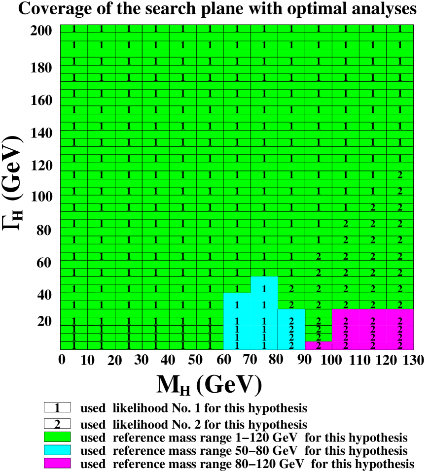
Figure 2: In total five analyses were used to cover the plane of hypothetical Higgs mass and decay width pairings. The analyses differ in whether the first or second likelihood was used (denoted by the number in the cell) and what signal masses where used in filling the reference histograms (depicted by the shading of the cell). The pattern resulted from an optimisation starting with $\Gamma_{\mathrm{H}}$ = 5 GeV up to 50 GeV. Below $\Gamma_{\mathrm{H}}$ = 5 GeV the pattern was simply continued and not optimised anymore. Above 50 GeV a simple continuation of the pattern was found and proved to be sufficiently sensitive.

References

- [1] R. Barate et al., ALEPH Collaboration, Phys. Lett. B 565, 61 (2003).
- [2] LEP Higgs Working Group, “Searches for invisible Higgs bosons: Preliminary combined results using LEP data collected at energies up to 209-GeV,” [arXiv:hep-ex/0107032].
- [3] G.F. Giudice, R. Rattazzi and J.D. Wells, Nucl. Phys. B 595, 250 (2001). M. Battaglia, D. Dominici, J.F. Gunion and J.D. Wells, “The invisible Higgs decay width in the ADD model at the LHC,” [arXiv:hep-ph/0402062].
- [4] T. Binoth and J.J. van der Bij, Z. Phys. C 75, 17 (1997).
- [5] G. Abbiendi et al., OPAL Collaboration, Eur. Phys. J. C 27, 311 (2003).
- [6] J.J. van der Bij, “The minimal non-minimal standard model,” [arXiv:hep-ph/0603082].
- [7] T. Binoth and J.J. van der Bij, “The stealthy Higgs model at future linear colliders,” [arXiv:hep-ph/9908256].
-
[8]
J.F. Gunion, H.E. Haber, G.L. Kane and S. Dawson, “The Higgs Hunter’s Guide,”
(Addison-Wesley, Reading MA, 1990), p.140. - [9] K. Ahmet et al., OPAL Collaboration, Nucl. Instr. and Meth. A 305, 275 (1991).
- [10] S. Anderson et al., Nucl. Instr. and Meth. A 403, 326 (1998).
- [11] G. Aguillon et. al., Nucl. Instr. and Meth. A 417, 266 (1998).
- [12] B.E. Anderson et al., IEEE Trans. on Nucl. Science 41, 845 (1994).
- [13] K. Ackerstaff et al., OPAL Collaboration, Phys. Lett. B 391, 221 (1997).
- [14] G. Abbiendi et al., OPAL Collaboration, Eur. Phys. J. C 26, 479 (2003).
- [15] N. Brown and W.J. Stirling, Phys. Lett. B 252, 657 (1990). G.D. Cowan, J. Phys. G 17, 1537 (1991). S. Catani, Y.L. Dokshitzer, M. Olsson, G. Turnock and B.R. Webber, Phys. Lett. B 269, 432 (1991). S. Bethke, Z. Kunszt, D.E. Soper and W.J. Stirling, Nucl. Phys. B 370, 310 (1992). [Erratum-ibid. B 523, 681 (1998)]. N. Brown and W.J. Stirling, Z. Phys. C 53, 629 (1992).
- [16] P. Janot, CERN 96-01, Vol.2, 309 (1996).
- [17] S. Jadach, B.F. Ward and Z.Wa̧s, Comp. Phys. Comm. 130, 260 (2000).
- [18] T. Sjöstrand, Comp. Phys. Comm. 82, 74 (1994). T. Sjöstrand, LU TP 95-20.
-
[19]
J. Fujimoto et al., Comp. Phys. Comm. 100, 128 (1997).
J. Fujimoto et al., CERN 96-01, Vol.2, 30 (1996). -
[20]
E. Budinov et al., CERN 96-01, Vol.2, 216 (1996).
R. Engel and J. Ranft, Phys. Rev. D 54, 4244 (1996). - [21] G. Marchesini et al., Comp. Phys. Comm. 67, 465 (1992).
- [22] J.A.M. Vermaseren, Nucl. Phys. B 229, 347 (1983).
- [23] J. Allison et al., OPAL Collaboration, Nucl. Instr. and Meth. A 317, 47 (1992).
- [24] M.Z. Akrawy et al., OPAL Collaboration, Phys. Lett. B 253, 511 (1991).
-
[25]
G. Abbiendi et al., OPAL Collaboration,
Phys. Lett. B 476, 256 (2000).
G. Abbiendi et al., OPAL Collaboration, Eur. Phys. J. C 32, 303 (2003). - [26] M. Acciarri et al., L3 Collaboration, Phys. Lett. B 485, 85 (2000).
- [27] G. Abbiendi et al., OPAL Collaboration, Eur. Phys. J. C 7, 407 (1999).
- [28] M.W. Grunewald et al., “Four-fermion production in electron positron collisions,” [arXiv:hep-ph/0005309].
- [29] A.L. Read, J. Phys. G 28 2693 (2002).
- [30] G. Abbiendi et al., OPAL Collaboration, Eur. Phys. J. C 40, 317 (2005).
- [31] T. Junk, Nucl. Instrum. Meth. A 434, 435 (1999).
- [32] R.D. Cousins and V.L. Highland, Nucl. Instrum. Meth. A 320, 331 (1992).