Observation of $B^{0}_{s}$-$\bar{B}^{0}_{s}$ Oscillations and
measurement of $\Delta m_{s}$ in CDF

Abstract

We report the observation of $B^{0}_{s}$-$\bar{B}^{0}_{s}$ oscillations performed by the CDF II detector using a data sample of 1 $\mathrm{fb^{-1}}$ of $p\bar{p}$ collisions at $\sqrt{s}=1.96~{}\rm Te\kern-1.00006ptV$. We measure the probability as a function of proper decay time that the $B_{s}$ decays with the same, or opposite, flavor as the flavor at production, and we find a signal for $B^{0}_{s}$-$\bar{B}^{0}_{s}$ oscillations. The probability that random fluctuations could produce a comparable signal is $8\times 10^{-8}$, which exceeds $5\sigma$ significance. We measure $\Delta m_{s}=17.77~{}\pm 0.10~{}({\rm stat})~{}\pm 0.07~{}({\rm syst})\,\mathrm{ps^{-1}}$. A very important update has been presented by the CDF collaboration after I gave my talk, the latest available results on $B_{s}$ mixing are included here.

1 Introduction

The precise determination of the $B^{0}_{s}$-$\bar{B}^{0}_{s}$ oscillation frequency $\Delta m_{s}$ from a time-dependent analysis of the $B^{0}_{s}$-$\bar{B}^{0}_{s}$ system has been one of the most important goals of heavy flavor physics [1]. This frequency can be used to strongly improve the knowledge of the Cabibbo-Kobayashi-Maskawa (CKM) matrix [2], and to constraint contributions from new physics [3].

Recently, the CDF collaboration reported [4] the strongest evidence to date of the direct observation of $B^{0}_{s}$-$\bar{B}^{0}_{s}$ oscillations, using a sample corresponding to 1 $\mathrm{fb^{-1}}$ of data collected with the CDF II detector [6] at the Fermilab Tevatron.

Here we report an update [5] of this measurement that uses the same data set with an improved analysis and reduces this probability to $8\times 10^{-8}$ ($>5\sigma$), yielding the definitive observation of time-dependent $B^{0}_{s}$-$\bar{B}^{0}_{s}$ oscillations.

The CDF analysis has been improved by increasing the $B_{s}$ signal yield and by improving the performance of the flavor tagging algorithms. We use $B_{s}$ decays in hadronic ($\bar{B}^{0}_{s}\to D^{+}_{s}\pi^{-}$, $D^{+}_{s}\pi^{-}\pi^{+}\pi^{-}$) and semileptonic ($\bar{B}^{0}_{s}\to D^{+(*)}_{s}\ell^{-}\bar{\nu}_{\ell}$, $\ell=e$ or $\mu$) modes (charge conjugates are always implied), with $D^{+}_{s}$ meson decaying in $D^{+}_{s}\rightarrow\phi\pi^{+}$, $\bar{K}^{*}(892)^{0}K^{+}$, and $\pi^{+}\pi^{-}\pi^{+}$, with $\phi\rightarrow K^{+}K^{-}$ and $\bar{K}^{*0}\rightarrow K^{-}\pi^{+}$. We improved signal yields by using particle identification techniques to find kaons from $D^{+}_{s}$ meson decays, allowing us to relax kinematic selection requirements, and by employing an artificial neural network (ANN) to improve candidate selection. Signal statistics is also significantly improved by adding partially reconstructed hadronic decays in which a photon or $\pi^{0}$ is missing: $\bar{B}^{0}_{s}\to D^{*+}_{s}\pi^{-}$, $D^{*+}_{s}\to D^{+}_{s}\gamma/\pi^{0}$ and $\bar{B}^{0}_{s}\to D^{+}_{s}\rho^{-}$, $\rho^{-}\to\pi^{-}\pi^{0}$, with $D^{+}_{s}\rightarrow\phi\pi^{+}$. Finally ANNs are used to enhance the power of the flavor tagging algorithms. With all these improvements, the effective statistical size of our data sample is increased respect to the previous published analysis by a factor of 2.5.

2 Data Sample

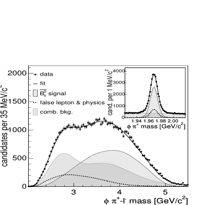
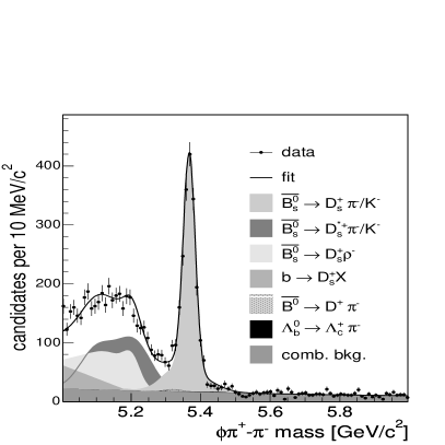
Figure 1: (Left:) The invariant mass distributions for the $D^{+}_{s}(\phi\pi^{+})$ candidates [inset] and the $\ell^{-}D^{+}_{s}(\phi\pi^{+})$ pairs. The contribution labelled “false lepton & physics” refers to backgrounds from hadrons mimicking the lepton signature combined with real $D_{s}$ mesons and other physics backgrounds. (Right:) The invariant mass distribution for $\bar{B}^{0}_{s}\to D^{+}_{s}(\phi\pi^{+})\pi^{-}$ decays including the contributions from partially reconstructed decays (signal contributions are drawn added on top of the combinatorial background).

$\bar{B}^{0}_{s}$ candidates are reconstructed by first selecting $D^{+}_{s}$ mesons that are lately combined with one or three additional charged particles to form $D^{+}_{s}\ell^{-}$, $D^{+}_{s}\pi^{-}$, or $D^{+}_{s}\pi^{-}\pi^{+}\pi^{-}$ candidates. Combinatorial background is reduced by cutting on the minimum $p_{T}$ of the $\bar{B}^{0}_{s}$ and its decay products, and by requirements on the quality of the reconstructed $\bar{B}^{0}_{s}$ and $D^{+}_{s}$ decay points and their displacement from the $p\bar{p}$ collision position. For decay modes with kaons in the final state, a kaon identification variable, formed by combining TOF and $dE/dx$ information, is used to reduce combinatorial background from random pions or from decays from $D^{+}$ meson. The distributions of the invariant masses of the $D_{s}^{+}(\phi\pi^{+})\ell^{-}$ pairs $m_{D_{s}\ell}$ and the $D_{s}^{+}(\phi\pi^{+})$ candidates are shown in Fig. 1. We use $m_{D_{s}\ell}$ to help distinguish signal, which occurs at higher $m_{D_{s}\ell}$, from combinatorial and physics backgrounds.

In this analysis, we also included partially reconstructed signal between 5.0 and 5.3 GeV/$c^{2}$ from $\bar{B}^{0}_{s}\to D^{*+}_{s}\pi^{-}$, $D^{*+}_{s}\to D^{+}_{s}\gamma/\pi^{0}$ in which a photon or $\pi^{0}$ from the $D^{*+}_{s}$ is missing and $\bar{B}^{0}_{s}\to D^{+}_{s}\rho^{-}$, $\rho^{-}\to\pi^{-}\pi^{0}$ in which a $\pi^{0}$ is missing. The mass distributions for $\bar{B}^{0}_{s}\to D^{+}_{s}\pi^{-}$, $D^{+}_{s}\rightarrow\phi\pi^{+}$ and the partially reconstructed signals are shown in Fig. 1. Table 1 summarizes the signal yields for the various decay modes.

Decay Sequence	Yield
$\bar{B}^{0}_{s}\to D^{+}_{s}\pi^{-}(\pi^{-}\pi^{+}\pi^{-})$	5600
$\bar{B}^{0}_{s}\to D^{+(*)}_{s}\ell^{-}\bar{\nu}_{\ell}$	61500
Partially reconstructed	3100

Table 1: Signal yields in hadronic, semileptonic and partially reconstructed decays.

We measure the proper decay time in the $B_{s}$ rest frame as $t=m_{B_{s}}L_{T}/p_{T}^{\rm recon}$, where $L_{T}$ is the measured displacement of the $B_{s}$ decay point with respect to the primary vertex projected onto the $B_{s}$ transverse momentum vector, and $p_{T}^{\rm recon}$ is the transverse momentum of the reconstructed decay products. In the semileptonic and partially reconstructed hadronic decays, we correct $t$ by a factor $\kappa=p_{T}^{\rm recon}/p_{T}(B_{s})$ determined with Monte Carlo simulation (Fig. 2). The decay time resolution $\sigma_{t}$ has contributions from the momentum of missing decay products (due to the spread of the distribution of $\kappa$) and from the uncertainty on $L_{T}$. The uncertainty due to the missing momentum increases with proper decay time and is an important contribution to $\sigma_{t}$ in the semileptonic decays. To reduce this contribution and make optimal use of the semileptonic decays, we determine the $\kappa$ distribution as a function of $m_{D_{s}\ell}$. The distribution of $\sigma_{t}$ for fully reconstructed decays has an average value of 87 fs, which corresponds to one fourth of an oscillation period at $\Delta m_{s}=17.8\,{\mathrm{ps^{-1}}}$, and an rms width of $31\,{\rm fs}$. For the partially reconstructed hadronic decays the average $\sigma_{t}$ is 97 fs, while for semileptonic decays, $\sigma_{t}$ is worse due to decay topology and the much larger missing momentum of decay products that were not reconstructed (see Fig. 2).

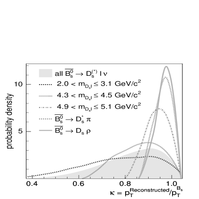
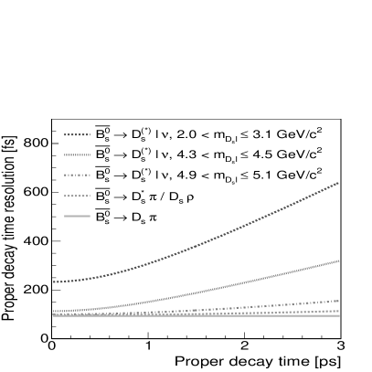
Figure 2: (Left:) The distribution of the correction factor $\kappa$ in semileptonic and partially reconstructed hadronic decays from Monte Carlo simulation. (Right:) The average proper decay time resolution for $B_{s}$ decays as a function of proper decay time.

3 Flavor Tagging

The flavor of the $\bar{B}^{0}_{s}$ at production is determined using both opposite-side and same-side flavor tagging techniques. The effectiveness $Q\equiv\epsilon{\cal D}^{2}$ of these techniques is quantified with an efficiency $\epsilon$, the fraction of signal candidates with a flavor tag, and a dilution ${\cal D}\equiv 1-2w$, where $w$ is the probability that the tag is incorrect. At the Tevatron, the dominant $b$-quark production mechanisms produce $b\bar{b}$ pairs.

Opposite-side tags infer the production flavor of the $\bar{B}^{0}_{s}$ from the decay products of the $b$ hadron produced from the other $b$ quark in the event. In this analysis we used lepton ($e$ and $\mu$) charge and jet charge as tags, and if both types of tag were present, we used the lepton tag. We also used an opposite-side flavor tag based on the charge of identified kaons, and we combine the information from the kaon, lepton, and jet charge tags using an ANN. The dilution is measured in data using large samples of $B^{-}$, which do not change flavor, and $\bar{B}^{0}$, which can be used after accounting for their well-known oscillation frequency. The combined opposite-side tag effectiveness is $Q=1.8\pm 0.1\,\%$.

Same-side flavor tags are based on the charges of associated particles produced in the fragmentation of the $b$ quark that produces the reconstructed $\bar{B}^{0}_{s}$. We use an ANN to combine kaon particle-identification likelihood with kinematic quantities of the kaon candidate into a single tagging variable. Tracks close in phase space to the $\bar{B}^{0}_{s}$ candidate are considered as same-side kaon tag candidates, and the track with the largest value of the tagging variable is selected as the tagging track. We predict the dilution of the same-side tag using simulated data samples generated with the pythia Monte Carlo [7] program. Control samples of $B^{-}$ and $\bar{B}^{0}$ are used to validate the predictions of the simulation. The effectiveness of this flavor tag is $Q=3.7\%$ ($4.8\%$) in the hadronic (semileptonic) decay sample. If both a same-side tag and an opposite-side tag are present, we combine the information from both tags assuming they are independent.

4 Fit and Results

We use an unbinned maximum likelihood fit to search for $B^{0}_{s}$-$\bar{B}^{0}_{s}$ oscillations. The likelihood combines mass, decay time, decay-time resolution, and flavor tagging information for each candidate, and includes terms for signal and each type of background. Following the method described in [8], we fit for the oscillation amplitude $\cal A$ while fixing $\Delta m_{s}$ to a probe value. The oscillation amplitude is expected to be consistent with ${\cal A}=1$ when the probe value is the true oscillation frequency, and consistent with ${\cal A}=0$ when the probe value is far from the true oscillation frequency. Figure 3 shows the fitted value of the amplitude as a function of the oscillation frequency for the semileptonic candidates alone, the hadronic candidates alone, and the combination. The sensitivity [4, 8] is 19.3 $\mathrm{ps^{-1}}$ for the semileptonic decays alone, 30.7 $\mathrm{ps^{-1}}$ for the hadronic decays alone, and 31.3 $\mathrm{ps^{-1}}$ for all decays combined. At $\Delta m_{s}=17.75~{}\mathrm{ps^{-1}}$, the observed amplitude ${\cal A}=1.21\pm 0.20~{}({\rm stat.})$ is consistent with unity, indicating that the data are compatible with $B^{0}_{s}$-$\bar{B}^{0}_{s}$ oscillations with that frequency, while the amplitude is inconsistent with zero: ${\cal A}/\sigma_{\cal A}=6.05$, where $\sigma_{\cal A}$ is the statistical uncertainty on ${\cal A}$ (the ratio has negligible systematic uncertainties). The small uncertainty on ${\cal A}$ at $\Delta m_{s}=17.75~{}\mathrm{ps^{-1}}$ is due to the superior decay-time resolution of the hadronic decay modes.

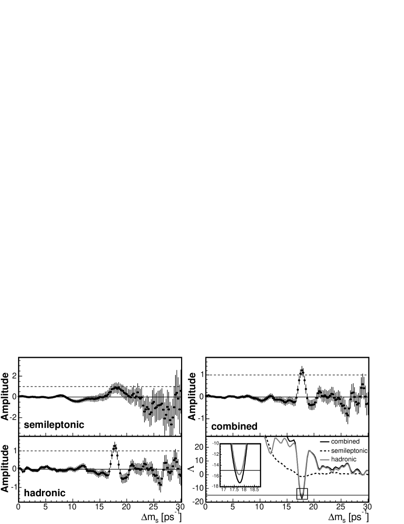
Figure 3: The measured amplitude values and uncertainties versus the $B^{0}_{s}$-$\bar{B}^{0}_{s}$ oscillation frequency $\Delta m_{s}$. (Upper Left) Semileptonic decays only. (Lower Left) Hadronic decays only. (Upper Right) All decay modes combined. (Lower Right) The logarithm of the ratio of likelihoods for amplitude equal to one and amplitude equal to zero versus the oscillation frequency.

We evaluate the significance of the signal using $\Lambda\equiv\log[{\cal L}^{{\cal A}=0}/{\cal L}^{{\cal A}=1}(\Delta m_{s})]$, which is the logarithm of the ratio of likelihoods for the hypothesis of oscillations (${\cal A}=1$) at the probe value and the hypothesis that ${\cal A}=0$, which is equivalent to random production flavor tags. Figure 3 shows $\Lambda$ as a function of $\Delta m_{s}$. Separate curves are shown for the semileptonic data alone (dashed), the hadronic data alone (light solid), and the combined data (dark solid). At the minimum $\Delta m_{s}=17.77~{}\mathrm{ps^{-1}}$, $\Lambda=-17.26$. The significance of the signal is the probability that randomly tagged data would produce a value of $\Lambda$ lower than $-17.26$ at any value of $\Delta m_{s}$. We repeat the likelihood scan 350 million times with random tagging decisions; 28 of these scans have $\Lambda<-17.26$, corresponding to a probability of $8\times 10^{-8}$ ($5.4\,\sigma$), well below $5.7\times 10^{-7}$ ($5\,\sigma$).

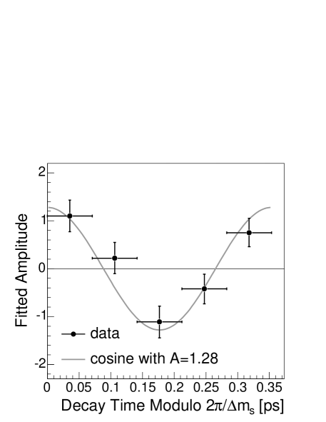
Figure 4: The $B^{0}_{s}$-$\bar{B}^{0}_{s}$ oscillation signal (only hadronic decays) measured in five bins of proper decay time modulo the measured oscillation period $2\pi/\Delta m_{s}$. The curve shown is a cosine with an amplitude of 1.28, which is the observed value in the amplitude scan for the hadronic sample at $\Delta m_{s}=17.77$ $\mathrm{ps^{-1}}$.

To measure $\Delta m_{s}$, we fix ${\cal A}=1$ and fit for the oscillation frequency. We find $\Delta m_{s}=17.77~{}\pm 0.10~{}({\rm stat})~{}\pm 0.07~{}({\rm syst})\,\mathrm{ps^{-1}}$.

The only non-negligible systematic uncertainty on $\Delta m_{s}$ is from the uncertainty on the absolute scale of the decay-time measurement.

The $B^{0}_{s}$-$\bar{B}^{0}_{s}$ oscillations are depicted in Fig. 4 where candidates in the hadronic sample are collected in five bins of proper decay time modulo the measured oscillation period $2\pi/\Delta m_{s}$.

References

- [1] C. Gay, Annu. Rev. Nucl. Part. Sci. 50, 577 (2000).
- [2] N. Cabibbo, Phys. Rev. Lett. 10, 531 (1963); M. Kobayashi and T. Maskawa, Prog. Theor. Phys. 49, 652 (1973).
- [3] See as example: UTFit Coll., M. Bona et al., hep-ph/0605213.
- [4] A. Abulencia et al. (CDF Collaboration), Phys. Rev. Lett. 97, 062003 (2006).
- [5] A. Abulencia et al. (CDF Collaboration), FERMILAB-PUB-06-344-E, hep-ex/0609040. Submitted to Phys. Rev. Lett.
- [6] D. Acosta et al. (CDF Collaboration), Phys. Rev. D 71, 032001 (2005); R. Blair et al. (CDF Collaboration), Fermilab Report No. FERMILAB–PUB–96–390–E, 1996; C. S. Hill et al., Nucl. Instrum. Methods Phys. Res., Sect. A 530, 1 (2004); S. Cabrera et al., Nucl. Instrum. Methods Phys. Res., Sect. A 494, 416 (2002); W. Ashmanskas et al., Nucl. Instrum. Methods Phys. Res., Sect. A 518, 532 (2004).
- [7] T. Sjöstrand et al., Computer Phys. Commun. 135, 238 (2001). We use version 6.216.
- [8] H. G. Moser and A. Roussarie, Nucl. Instrum. Methods Phys. Res., Sect. A 384, 491 (1997).