Measurement of $\phi_{3}$ with Dalitz Plot Analysis of $B^{+}\to D^{(*)}K^{(*)+}$  Decay

Abstract

Results from the Belle and BaBar experiments on measurement of the weak angle $\phi_{3}$ using a Dalitz plot analysis of the $K^{0}_{S}\pi^{+}\pi^{-}$ decay of the neutral $D$ meson from the $B^{\pm}\to D^{(*)}K^{(*)\pm}$ process are presented. The method employs the interference between $D^{0}$ and $\overline{D}{}^{0}$ to extract the angle $\phi_{3}$, strong phase $\delta$ and the ratio $r$ of suppressed and allowed amplitudes.

1 Introduction

Determinations of the Cabibbo-Kobayashi-Maskawa matrix elements provide important checks on the consistency of the standard model and ways to search for new physics. The possibility of observing direct $CP$ violation in $B\to DK$ decays was first discussed by I. Bigi, A. Carter and A. Sanda [1]. Since then, various methods to measure the weak angle $\phi_{3}$ (also known as $\gamma$) using $B\to DK$ decays have been proposed. All these methods are based on two key observations: neutral $D^{0}$ and $\overline{D}{}^{0}$ mesons can decay to a common final state, and the decay $B^{+}\to DK^{+}$ can produce neutral $D$ mesons of both flavors via $\bar{b}\to\bar{c}u\bar{s}$ and $\bar{b}\to\bar{u}c\bar{s}$ transitions, with a relative phase $\theta_{+}$ between the two interfering amplitudes that is the sum, $\delta+\phi_{3}$, of strong and weak interaction phases. For the decay $B^{-}\to DK^{-}$, the relative phase is $\theta_{-}=\delta-\phi_{3}$, so both phases can be extracted from measurements of such charge conjugate $B$ decay modes. (Unless stated otherwise charge conjugation is implied throughout this report.) However, the use of branching fractions alone requires additional information to obtain $\phi_{3}$. This is provided either by determining the branching fractions of decays to $CP$ eigenstates (GLW method [2]) or by using different neutral $D$ final states (ADS method [3]).

A Dalitz plot analysis of a three-body final state of the $D$ meson allows one to obtain all the information required for determination of $\phi_{3}$ in a single decay mode. Three body final states such as $K^{0}_{S}\pi^{+}\pi^{-}$ have been suggested [4, 5] as promising modes for the extraction of $\phi_{3}$. In the Wolfenstein parameterization of the CKM matrix elements, the weak parts of the amplitudes that contribute to the decay $B^{+}\to DK^{+}$ are given by $V_{cb}^{*}V_{us\vphantom{b}}^{\vphantom{*}}\sim A\lambda^{3}$ (for the $\overline{D}{}^{0}K^{+}$ final state) and $V_{ub}^{*}V_{cs\vphantom{b}}^{\vphantom{*}}\sim A\lambda^{3}(\rho+i\eta)$ (for $D^{0}K^{+}$). The two amplitudes interfere as the $D^{0}$ and $\overline{D}{}^{0}$ mesons decay into the same final state $K^{0}_{S}\pi^{+}\pi^{-}$; the admixed state is denoted as $\tilde{D}_{\pm}$. Assuming no $CP$ asymmetry in neutral $D$ decays, the amplitude of the $\tilde{D}_{\pm}$ decay as a function of Dalitz plot variables $m^{2}_{+}=m^{2}_{K^{0}_{S}\pi^{+}}$ and $m^{2}_{-}=m^{2}_{K^{0}_{S}\pi^{-}}$ is

$$M_{\pm}=f(m^{2}_{\pm},m^{2}_{\mp})+re^{\pm i\phi_{3}+i\delta}f(m^{2}_{\mp},m^{2}_{\pm}),$$ (1)

where $f(m^{2}_{+},m^{2}_{-})$ is the amplitude of the $\overline{D}{}^{0}$$\to$$K^{0}_{S}\pi^{+}\pi^{-}$ decay, and $r$ is the ratio of the magnitudes of the two interfering amplitudes. The value of $r$ is given by the ratio of the CKM matrix elements $|V_{ub}^{*}V_{cs\vphantom{b}}^{\vphantom{*}}|/|V_{cb}^{*}V_{us\vphantom{b}}^{\vphantom{*}}|$ and the color suppression factor, and is estimated to be in the range 0.1–0.2 [6].

The method has a two-fold ambiguity: the $(\phi_{3},\delta)$ and $(\phi_{3}+180^{\circ},\delta+180^{\circ})$ solutions cannot be separated. The solution with $0<\phi_{3}<180^{\circ}$ is chosen.

The method described above can be applied to other $B$ decay modes such as $B^{+}\to D^{*}K^{+}$ and $B^{+}\to DK^{*+}$.

2 Data Samples

Results from the two $B$-factories Belle/KEKB and BaBar/PEPII are available. The current proceedings are based on results reported in Refs. [7, 8]. For the most recent updates see Ref. [9]. The Belle collaboration uses a data sample that consists of $386\times 10^{6}$ $B\bar{B}$ pairs. The decay chains $B^{+}\to DK^{+}$, $B^{+}\to D^{*}K^{+}$ with $D^{*}$$\to$$D\pi^{0}$ and $B^{+}\to DK^{*+}$ with $K^{*+}$$\to$$K^{0}_{S}\pi^{+}$ are selected for the analysis. Analysis by the BaBar collaboration is based on $227\times 10^{6}$ $B\bar{B}$ pairs. The reconstructed final states are $B^{+}\to DK^{+}$and $B^{+}\to D^{*}K^{+}$with two $D^{*}$ channels: $D^{*}$$\to$$D\pi^{0}$ and $D^{*}$$\to$$D\gamma$. The neutral $D$ meson is reconstructed in the $K^{0}_{S}\pi^{+}\pi^{-}$ final state in all cases. The dominant backgrounds come from a random combination of a real or fake $D^{(*)0}$ meson with a charged track in continuum events; from $B^{+}\to D^{(*)}\pi^{+}$ events with $\pi-K$ misidentification or other $B\bar{B}$ decays.

Table 1: Fit results for $\overline{D}{}^{0}$$\to$$K^{0}_{S}\pi^{+}\pi^{-}$ decay [7].

Channel	Phase (∘)	Fit fraction
$K^{0}_{S}\sigma_{1}$	$212\pm 3$	9.8%
$K^{0}_{S}\rho^{0}$	0 (fixed)	21.6%
$K^{0}_{S}\omega$	$110.8\pm 1.6$	0.4%
$K^{0}_{S}f_{0}(980)$	$201.9\pm 1.9$	4.9%
$K^{0}_{S}\sigma_{2}$	$237\pm 11$	0.6%
$K^{0}_{S}f_{2}(1270)$	$348\pm 2$	1.5%
$K^{0}_{S}f_{0}(1370)$	$82\pm 6$	1.1%
$K^{0}_{S}\rho^{0}(1450)$	$9\pm 8$	0.4%
$K^{*}(892)^{+}\pi^{-}$	$132.1\pm 0.5$	61.2%
$K^{*}(892)^{-}\pi^{+}$	$320.3\pm 1.5$	0.55%
$K^{*}(1410)^{+}\pi^{-}$	$113\pm 4$	0.05%
$K^{*}(1410)^{-}\pi^{+}$	$254\pm 5$	0.14%
$K_{0}^{*}(1430)^{+}\pi^{-}$	$353.6\pm 1.2$	7.4%
$K_{0}^{*}(1430)^{-}\pi^{+}$	$88\pm 4$	0.43%
$K_{2}^{*}(1430)^{+}\pi^{-}$	$318.7\pm 1.9$	2.2%
$K_{2}^{*}(1430)^{-}\pi^{+}$	$265\pm 6$	0.09%
$K^{*}(1680)^{+}\pi^{-}$	$103\pm 12$	0.36%
$K^{*}(1680)^{-}\pi^{+}$	$118\pm 11$	0.11%
non-resonant	$164\pm 5$	9.7%

The numbers of reconstructed signal events in the Belle’s sample are $331\pm 23$, $81\pm 11$ and $54\pm 8$ for the $B^{+}\to DK^{+}$, $B^{+}\to D^{*}K^{+}$and $B^{+}\to DK^{*+}$channels, respectively. BaBar finds $282\pm 20$, $90\pm 11$ and $44\pm 8$ signal events in the $B^{+}\to DK^{+}$, $B^{+}\to D^{*}[D\pi^{0}]K^{+}$ and $B^{+}\to D^{*}[D\gamma]K^{+}$ respectively.

Several high statistics control samples are reconstructed in order to cross-check the $CP$ fit results. A sample of $D^{*-}\to\overline{D}{}^{0}\pi^{-}$ events produced via the $e^{+}e^{-}\to c\bar{c}$ continuum process is selected. This decay mimics the $B^{-}\to D^{0}K^{-}$ decay with $r=0$. The $B^{+}\to D^{(*)}\pi^{+}$ mode is used as a second control sample where $r$ is expected to be approximately 0.01.

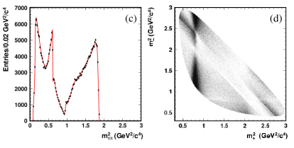
Figure 1: (a) $m^{2}_{-}$, (b) $m^{2}_{+}$, (c) $m^{2}_{\pi\pi}$ and (d) Dalitz plot distribution for $D^{*-}\to\overline{D}{}^{0}\pi^{-}$, $\overline{D}{}^{0}$$\to$$K^{0}_{S}\pi^{+}\pi^{-}$ decays from the $e^{+}e^{-}\to c\bar{c}$ continuum process. The points with error bars show the data; the smooth curve is the fit result [7].

3 $\overline{D}{}^{0}$$\to$$K^{0}_{S}\pi^{+}\pi^{-}$ decay amplitude

The $\overline{D}{}^{0}$$\to$$K^{0}_{S}\pi^{+}\pi^{-}$ decay amplitude $f(m^{2}_{+},m^{2}_{-})$ can be determined independently from a large sample of flavor-tagged $D^{*-}\to\overline{D}{}^{0}\pi^{-}$, $\overline{D}{}^{0}$$\to$$K^{0}_{S}\pi^{+}\pi^{-}$ decays produced in continuum $e^{+}e^{-}$ annihilation. Once $f$ is known, a fit to $B^{\pm}$ data allows determination of $r$, $\phi_{3}$ and $\delta$.

The amplitude $f$ is parametrized as a coherent sum of quasi-two-body amplitudes $\mathcal{A}_{j}$ and a non-resonant amplitude,

$$f(m^{2}_{+},m^{2}_{-})=\sum\limits_{j=1}^{N}a_{j}e^{i\alpha_{j}}\mathcal{A}_{j}(m^{2}_{+},m^{2}_{-})+be^{i\beta},$$ (2)

where $N$ is the total number of resonances and $a_{j}$, $\alpha_{j}$, $b$ and $\beta$ are free parameters. A set of 18 quasi-two-body amplitudes is used to fit the data. The list of resonances included in the model as well as parameters determined from the fit are summarized in Table 1. For consistency with other analyzes [8, 10], the $\overline{D}{}^{0}\to K^{0}_{S}\rho^{0}$ mode is chosen to have unit amplitude and zero relative phase. The $\overline{D}{}^{0}$$\to$$K^{0}_{S}\pi^{+}\pi^{-}$ Dalitz plot distribution, as well as its projections with the fit results superimposed, are shown in Fig. 1.

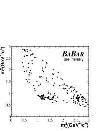
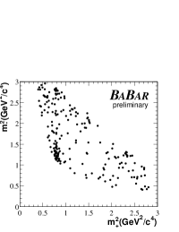
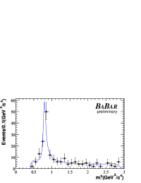
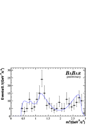
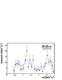
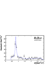
Figure 2: Dalitz plot and one dimensional projections for the $B^{-}\to D^{0}K^{-}$ (left column) and $B^{+}\to\bar{D}^{0}K^{+}$ candidates (right column) in the $B$ signal region [8].

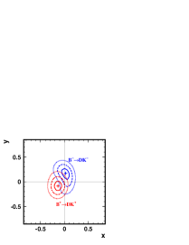
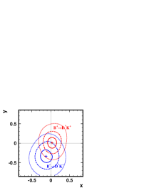
Figure 3: Results of signal fits with free parameters $x=r\cos\theta$ and $y=r\sin\theta$ for (a) $B^{+}\to DK^{+}$and (b) $B^{+}\to D^{*}K^{+}$ samples, separately for $B^{-}$ and $B^{+}$ data. Contours indicate integer multiples of the standard deviation [7].

4 $CP$ Analysis

Analysis of $CP$ violation is performed by means of a maximum likelihood fit. The fit is performed by minimizing the negative likelihood function (Belle performs an unbinned fit while BaBar uses a binned approach.)

$$-2\log L=-2\sum\limits^{n}_{i=1}\log p(m^{2}_{+,i},m^{2}_{-,i},\Delta E_{i},M_{{\rm bc},i}),$$ (3)

with the Dalitz plot density $p$ represented as

$$p(m^{2}_{+},m^{2}_{-},\Delta E,M_{\rm bc})=~{}~{}~{}~{}~{}~{}~{}~{}~{}~{}~{}~{}~{}~{}~{}~{}~{}~{}~{}~{}~{}~{}~{}~{}~{}~{}~{}~{}~{}~{}~{}~{}~{}~{}$$

$$\varepsilon|f(m^{2}_{+},m^{2}_{-})+(x+iy)f(m^{2}_{-},m^{2}_{+})|^{2}F_{\rm sig}(\Delta E,M_{\rm bc})$$

$$~{}~{}~{}~{}~{}~{}~{}~{}~{}~{}~{}~{}~{}~{}~{}~{}~{}~{}~{}~{}+F_{\rm bck}(m^{2}_{+},m^{2}_{-},\Delta E,M_{\rm bc}),$$ (4)

where $x=r\cos(\phi_{3}+\delta)$, $y=r\sin(\phi_{3}+\delta)$; $F_{\rm sig}$ is the signal $\Delta E$ and $M_{\rm bc}$ distribution represented by the product of two Gaussian functions (BaBar also includes Fisher discriminant in the fit); $F_{\rm bck}$ is the distribution of the background events, and $\varepsilon=\varepsilon(m^{2}_{+},m^{2}_{-})$ is reconstruction efficiency determined from MC simulation. The background density function $F_{\rm bck}$ is determined from analysis of sideband events in data and with Monte Carlo generated events.

The fit procedure is first tested on two high statistics control samples: $D^{*+}$$\to$$D^{0}\pi^{+}$ from $c\bar{c}$ continuum events and $B^{-}$$\to$$D^{(*)0}\pi^{-}$. In the $CP$ fit to $D^{*+}$$\to$$D^{0}\pi^{+}$ the fit yields $r_{B}=(-5.2\pm 5.2)\times 10^{-3}$. Results consistent with $r=0$ are obtained with the other two control samples: $r_{B}=(1.8\pm 1.5)\times 10^{-2}$ for the $B^{-}$$\to$$D^{0}\pi^{-}$ mode and $r_{D^{*}K}=(4.6\pm 2.1)\times 10^{-2}$ for the $B^{-}$$\to$$D^{*0}\pi^{-}$ mode. This is in agreement with expectations.

Table 2: Summary of fits results.

Parameter	Belle	BaBar
$\phi_{3}$	$53.3^{+14.8}_{-17.7}\pm 2.5\pm 8.7$	$70\pm 31^{+12+14}_{-10-11}$
$r_{DK}$	$0.159^{+0.054}_{-0.050}\pm 0.012\pm 0.049$	$0.12\pm 0.08\pm 0.03\pm 0.04$
$\delta_{DK}$	$145.7^{+19.0}_{-19.7}\pm 3.0\pm 22.9$	$104\pm 45^{+17+16}_{-21-24}$
$r_{D^{*}K}$	$0.175^{+0.108}_{-0.099}\pm 0.013\pm 0.049$	$0.17\pm 0.10\pm 0.03\pm 0.03$
$\delta_{D^{*}K}$	$302.0^{+33.8}_{-35.1}\pm 6.1\pm 22.9$	$296\pm 41^{+14}_{-12}\pm 15$
$r_{DK^{*}}$	$0.564^{+0.216}_{-0.155}\pm 0.041\pm 0.084$	$-$
$\delta_{DK^{*}}$	$242.6^{+20.2}_{-23.2}\pm 2.5\pm 49.3$	$-$

A summary of the results of the fits to the signal events is given in Table 2, where the first quoted error is statistical, the second is systematic and the third is a model uncertainty. Figure 3 demonstrates results of the fit to $B^{+}\to DK^{+}$ and $B^{+}\to D^{*}K^{+}$ events on the $x-y$ plane.

Systematic errors come from uncertainty in the knowledge of the functions used in the signal Dalitz plot fit. These include the Dalitz plot profiles of the backgrounds and the detection efficiency, the momentum resolution description, and on the parametrization of the $\Delta E-M_{\rm bc}$ shape of the signal and background. Though the statistical error is still quite large, this method currently provides the best direct constraints on $\phi_{3}$.

Uncertainty in the model used to parametrize the $\overline{D}{}^{0}$$\to$$K^{0}_{S}\pi^{+}\pi^{-}$ decay amplitude is the source of the associated error in the analysis. It arises from a non-unique choice of the set of quasi-two-body channels as well as uncertainty in parametrization of some components (non-resonant amplitude, for example). To evaluate this uncertainty several alternative models have been used to fit the data.

Although at present the $\phi_{3}$ accuracy is dominated by the statistical uncertainty, the model error will eventually dominate as the experimental statistics increase. A model independent way to extract $\phi_{3}$ has been proposed in Ref. [4]. The idea is that in addition to flavor tagged $\overline{D}{}^{0}$$\to$$K^{0}_{S}\pi^{+}\pi^{-}$ decays, one can use $CP$ tagged decays to $K^{0}_{S}\pi^{+}\pi^{-}$ from the $\psi(3770)\to D\bar{D}$ process. Combining the two data sets the amplitude and phase could be measured for each point on the Dalitz plot in a model independent way. Study with Monte Carlo simulations indicates that with with 50 ab^-1 of data $\phi_{3}$ can be measured with a total accuracy of better than 2 degrees.

References

[1]
I. I. Bigi and A. I. Sanda, Phys. Lett. B211, 213 (1988);
A. B. Carter and A. I. Sanda, Phys. Rev. Lett 45, 952 (1980).
[2]
M. Gronau and D. London, Phys. Lett. B253, 483 (1991);
M. Gronau and D. Wyler, Phys. Lett. B265, 172 (1991).
[3]
D. Atwood, I. Dunietz and A. Soni, Phys. Rev. Lett. 78, 3257 (1997);
D. Atwood, I. Dunietz and A. Soni, Phys. Rev. D 63, 036005 (2001).
[4]
A. Giri, Yu. Grossman, A. Soffer, J. Zupan, Phys. Rev. D 68,
054018 (2003).
[5]
A. Bondar. Proceedings of BINP Special Analysis Meeting on Dalitz Analysis,
24-26 Sep. 2002, unpublished.
[6]
M. Gronau, Phys. Lett. B557, 198 (2003).
[7]
Belle Collaboration, A. Poluektov et al.,
Phys. Rev. D 73, 112009 (2006).
[8]
BABAR Collaboration, B. Aubert et al.,
Phys. Rev. Lett. 95, 121802 (2005).
[9]
Heavy Flavor Averaging Group:
www.slac.stanford.edu/xorg/hfag/.
[10]
CLEO Collaboration, H. Muramatsu et al., Phys. Rev. Lett.
89, 251802 (2002), Erratum-ibid: 90, 059901 (2003).