MEASUREMENT OF $D_{s}^{+}\to\ell^{+}\nu$ AND THE DECAY CONSTANT $f_{D_{s}}$

Abstract

I report preliminary CLEO-c results on purely leptonic decays of the $D_{s}$ using 195 pb^-1 of data at 4.170 GeV. We measure $f_{D_{s}}=280.1\pm 11.6\pm 6.0{~{}\rm MeV}$, and $f_{D_{s}^{+}}/{f_{D^{+}}=1.26\pm 0.11\pm 0.03}$.

1 Introduction

To extract precise information from $B-\overline{B}$ mixing measurements the ratio of “leptonic decay constants,” $f_{i}$ for $B_{d}$ and $B_{s}$ mesons must be well known.[1] Indeed, the recent measurement of $B_{s}^{0}-\overline{B}_{s}^{0}$ mixing by CDF[2] has pointed out the urgent need for precise numbers. The $f_{i}$ have been calculated theoretically. The most promising of these calculations are based on lattice-gauge theory that include the light quark loops.[3] In order to ensure that these theories can adequately predict $f_{B_{s}}/f_{B_{d}}$ it is critical to check the analogous ratio from charm decays $f_{D^{+}_{s}}/f_{D^{+}}$. We have previously measured $f_{D^{+}}$.[4, 5] Here I present the most precise measurements to date of $f_{D_{s}^{+}}$ and $f_{D_{s}^{+}}/f_{D^{+}}$.

In the Standard Model (SM) the $D_{s}$ meson decays purely leptonically, via annihilation through a virtual $W^{+}$, as shown in Fig. 1. The decay width is given by[6]

$$\Gamma(D_{s}^{+}\to\ell^{+}\nu) = {{G_{F}^{2}}\over 8\pi}f_{D_{s}^{+}}^{2}m_{\ell^{+}}^{2}M_{D_{s}^{+}}$$

$$\times\left(1-{m_{\ell^{+}}^{2}\over M_{D_{s}^{+}}^{2}}\right)^{2}\left|V_{cs}\right|^{2}~{},$$

where $m_{\ell^{+}}$ and $M_{D_{s}^{+}}$ are the $\ell^{+}$ and $D_{s}^{+}$ masses, $|V_{cs}|$ is a CKM element equal to 0.9737, and $G_{F}$ is the Fermi constant.

Figure 1: The decay diagram for $D_{s}^{+}\to\ell^{+}\nu$.

New physics can affect the expected widths; any undiscovered charged bosons would interfere with the SM $W^{+}$. These effects may be difficult to ascertain, since they would simply change the value of $f_{i}$ extracted using Eq. (1). We can, however, measure the ratio of decay rates to different leptons, and the predictions then are fixed only by well-known masses. For example, for $\tau^{+}\nu$ to $\mu^{+}\nu$:

$$R\equiv\frac{\Gamma(D\to\tau^{+}\nu)}{\Gamma(D\to\mu^{+}\nu)}={{m_{\tau^{+}}^{2}\left(1-{m_{\tau^{+}}^{2}\over M_{D}^{2}}\right)^{2}}\over{m_{\mu^{+}}^{2}\left(1-{m_{\mu^{+}}^{2}\over M_{D}^{2}}\right)^{2}}}~{}~{}.$$ (2)

Any deviation from this formula would be a manifestation of physics beyond the SM. This could occur if any other charged intermediate boson existed that coupled to leptons differently than mass-squared. Then the couplings would be different for muons and $\tau$’s. This would be a clear violation of lepton universality.[7]

2 Experimental Method

In this study we use 195 pb^-1 of data produced in $e^{+}e^{-}$ collisions using the Cornell Electron Storage Ring (CESR) and recorded near 4.170 GeV. Here the cross-section for $D_{s}^{*+}D_{s}^{-}$+$D_{s}^{+}D_{s}^{*-}$ is $\sim$1 nb. We fully reconstruct one $D_{s}$ as a “tag,” and examine the properties of the other. In this paper we designate the tag as a $D_{s}^{-}$ and examine the leptonic decays of the $D_{s}^{+}$, though in reality we use both charges. Track selection, particle identification, $\gamma$, $\pi^{0}$, $K_{S}$ and muon selection cuts are identical to those described in Artuso et al.[4]

The $D_{s}^{-}$ decay modes used for tagging are listed in Table 2. The number of signal and background events are determined by fits to the invariant mass distributions.

Tagging modes and numbers of signal and background events, within $\pm 2.5\sigma$ for all modes, except $\eta\rho^{+}$ ($\pm 2\sigma$), from two-Gaussian fits to the invariant mass plots. Mode Signal Background $K^{+}K^{-}\pi^{-}$ $8446\pm 160$ 6792 $K_{S}K^{-}$ 1852$\pm$62 1021 $\eta\pi^{-}$; $\eta\to\gamma\gamma$ $1101\pm 80$ 2803 $\eta^{\prime}\pi^{-}$; $\eta^{\prime}\to\pi^{+}\pi^{-}\eta$ 786$\pm$37 242 $\phi\rho^{-}$ 1140$\pm$59 1515 $\pi^{+}\pi^{-}\pi^{-}$ 2214$\pm$156 15668 $K^{*-}\overline{K}^{*0}$ 1197$\pm$81 2955 $\eta\rho^{-}$ 2449$\pm$185 13043 Sum $19185\pm 325$ 44039

We search for three separate decay modes: $D_{s}^{+}\to\mu^{+}\nu$, $D_{s}^{+}\to\tau^{+}\nu$, $\tau^{+}\to\pi^{+}\overline{\nu}$ and $\tau^{+}\to e^{+}\nu\overline{\nu}$. For the first two analyses we require the detection of the $\gamma$ from the $D_{s}^{*}\to\gamma D_{s}$ decay. Regardless of whether or not the photon forms a $D_{s}^{*}$ with the tag, for real $D_{s}^{*}D_{s}$ events, the missing mass squared recoiling against the photon and the $D_{s}^{-}$ tag should peak at the $D_{s}^{+}$ mass and is given by

$${\rm MM}^{*2}=\left(E_{\rm CM}-E_{D}-E_{\gamma}\right)^{2}-\left(-\overrightarrow{p_{D}}-\overrightarrow{p_{\gamma}}\right)^{2},$$

where $E_{\rm CM}$ is the center of mass energy, $E_{D}$ ($\overrightarrow{p_{D}}$) and $E_{\gamma}$ ($\overrightarrow{p_{\gamma}}$) are the energy (momentum) of the fully reconstructed $D_{s}^{-}$ tag, and the additional photon. In performing this calculation we use a kinematic fit that constrains the decay products of the $D_{s}^{-}$ to the known $D_{s}$ mass and conserves overall momentum and energy.

The MM^∗2 from the $D_{s}^{-}$ tag sample data is shown in Fig. 2. Fitting shows a yield of 12604$\pm$423 signal events. Restricting to the interval $3.978>$MM${}^{*2}>3.776$ GeV², we are left with 11880$\pm$399 events. The systematic error is $\pm$4.3%.

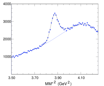
Figure 2: The MM*² distribution from events with a photon in addition to the $D_{s}^{-}$ tag. The curve is a fit to the Crystal Ball function and a 5th order Chebychev background function.

Candidate $D_{s}^{+}\to\mu^{+}\nu$ events are searched for by selecting events with only a single extra track with opposite sign of charge to the tag; we also require that there not be an extra neutral energy cluster in excess of 300 MeV. Since here we are searching for events where there is a single missing neutrino, the missing mass squared, MM², evaluated by taking into account the seen $\mu^{+}$, $D_{s}^{-}$, and the $\gamma$ should peak at zero, and is given by

$${\rm MM}^{2} = \left(E_{\rm CM}-E_{D}-E_{\gamma}-E_{\mu}\right)^{2}$$

$$-\left(-\overrightarrow{p_{D}}-\overrightarrow{p_{\gamma}}-\overrightarrow{p_{\mu}}\right)^{2},$$

where $E_{\mu}$ ($\overrightarrow{p_{\mu}}$) is the energy (momentum) of the candidate muon track.

We also make use of a set of kinematical constraints and fit the MM² for each $\gamma$ candidate to two hypotheses one of which is that the $D_{s}^{-}$ tag is the daughter of a $D_{s}^{*-}$ and the other that the $D_{s}^{*+}$ decays into $\gamma D_{s}^{+}$, with the $D_{s}^{+}$ subsequently decaying into $\mu^{+}\nu$. The hypothesis with the lowest $\chi^{2}$ is kept. If there is more than one $\gamma$ candidate in an event we choose only the lowest $\chi^{2}$ choice among all the candidates and hypotheses.

The kinematical constraints are the total momentum and energy, the energy of the either the $D_{s}^{*}$ or the $D_{s}$, the appropriate $D_{s}^{*}-D_{s}$ mass difference and the invariant mass of the $D_{s}$ tag decay products. This gives us a total of 7 constraints. The missing neutrino four-vector needs to be determined, so we are left with a three-constraint fit. We preform a standard iterative fit minimizing $\chi^{2}$. As we do not want to be subject to systematic uncertainties that depend on understanding the absolute scale of the errors, we do not make a $\chi^{2}$ cut, but simply choose the photon and the decay sequence in each event with the minimum $\chi^{2}$.

We consider three separate cases: (i) the track deposits $<$ 300 MeV in the calorimeter, characteristic of a non-interacting $\pi^{+}$ or a $\mu^{+}$; (ii) the track deposits $>$ 300 MeV in the calorimeter, characteristic of an interacting $\pi^{+}$; (iii) the track satisfies our $e^{+}$ selection criteria.[4] Then we separately study the MM² distributions for these three cases. The separation between $\mu^{+}$ and $\pi^{+}$ is not unique. Case (i) contains 99% of the $\mu^{+}$ but also 60% of the $\pi^{+}$, while case (ii) includes 1% of the $\mu^{+}$ and 40% of the $\pi^{+}$.[5]

Figure 3: The MM² distributions from data using $D_{s}^{-}$ tags and one additional opposite-sign charged track and no extra energetic showers (see text). (a) Case (i) the single track deposits $<$ 300 MeV of energy in the calorimeter. The peak near zero is from $D_{s}^{+}\to\mu^{+}\nu$ events. (b) Case (ii) Track deposits $>$ 300 MeV in crystal calorimeter but is not consistent with being an $e^{+}$. (c) Case (iii) the track is identified as an $e^{+}$.

The overall signal region we consider is below MM² of 0.20 GeV². Otherwise we admit background from $\eta\pi^{+}$ and $K^{0}\pi^{+}$ final states. There is a clear peak in Fig. 3(i), due to $D_{s}^{+}\to\mu^{+}\nu$. Furthermore, the events in the region between $\mu^{+}\nu$ peak and 0.20 GeV² are dominantly due to the $\tau^{+}\nu$ decay.

The specific signal regions are defined as follows: for $\mu^{+}\nu$, $0.05>$MM${}^{2}>-0.05$ GeV², corresponding to $\pm 2\sigma$ or 95% of the signal; for $\tau\nu$, $\tau^{+}\to\pi^{+}\overline{\nu}$, in case (i) $0.20>$MM${}^{2}>0.05$ GeV² and in case (ii) $0.20>$MM${}^{2}>-0.05$ GeV². In these regions we find 64, 24 and 12 events, respectively. The corresponding backgrounds are estimated as 1, 2.5 and 1 event, respectively. The branching fractions are summarized in Table 2. The absence of any detected $e^{+}$ opposite to our tags allows us to set the upper limit listed in Table 2.

Measured $D_{s}^{+}$ Branching Fractions Final State ${\cal{B}}$ (%) $\mu^{+}\nu$ $0.657\pm 0.090\pm 0.028$ $\mu^{+}\nu^{\dagger}$ $0.664\pm 0.076\pm 0.028$ $\tau^{+}\nu,~{}(\tau^{+}\to\pi^{+}\nu)$ $7.1\pm 1.4\pm 0.3$ $\tau^{+}\nu,~{}(\tau^{+}\to e^{+}\nu\bar{\nu})$ $6.29\pm 0.78\pm 0.52$ $\tau^{+}\nu$ (average) $6.5\pm 0.8$ $e^{+}\nu$ $<3.1\times 10^{-4}$ (90% cl) $\dagger$ From summing the $\mu^{+}\nu$ and $\tau^{+}\nu$ contributions for MM² $<$ 0.20 GeV².

The $D_{s}^{+}\to\tau^{+}\nu$, $\tau^{+}\to e^{+}\nu\overline{\nu}$ mode is measured by detecting electrons of opposite sign to the tag in events without any additional charged tracks, and determining the unmatched energy in the crystal calorimeter (${\rm E^{extra}_{CC}}$). This energy distribution is shown in Fig. 4. Requiring ${\rm E^{extra}_{CC}<}$ 400 MeV, enhances the signal. The branching ratio resulting from this analysis is listed in Table 2.

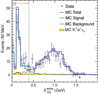
Figure 4: The extra calorimeter energy from data (points), compared with the Monte Carlo simulated estimates of semileptonic decays in general (dotted), the $K^{0}e^{+}\nu$ mode specifically (shaded), as a sub-set of the semileptonics, and the expectation from signal (dashed). The peak near 150 MeV is due to the $\gamma$ from $D_{s}^{*}\to\gamma D_{s}$ decay. (The sum is also shown (line).) The arrow indicates the selected signal region below 0.4 GeV.

3 Conclusions

Lepton universality in the SM requires that the ratio $R$ from Eq. 2 be equal to a value of 9.72. We measure

$$R\equiv\frac{\Gamma(D_{s}^{+}\to\tau^{+}\nu)}{\Gamma(D_{s}^{+}\to\mu^{+}\nu)}=9.9\pm 1.9~{}.$$ (4)

Thus we see no deviation from the predicted value. Current results on $D^{+}$ leptonic decays also show no deviations.[8] Combining all three branching ratios determinations and using $\tau_{D_{s}^{+}}$=0.49 ps to find the leptonic width, we find

$$f_{D_{s}}=280.1\pm 11.6\pm 6.0{~{}\rm MeV}.$$ (5)

Using our previous result[4]

$$f_{D}^{+}=222.6\pm 16.7^{+2.8}_{-3.4}{\rm~{}MeV,}$$ (6)

provides a determination of

$${{f_{D_{s}^{+}}}/{f_{D^{+}}}=1.26\pm 0.11\pm 0.03}.$$ (7)

These preliminary results are consistent with most recent theoretical models. As examples, unquenched lattice[9] predicts $1.24\pm 0.01\pm 0.07$, while one quenched lattice calculation[10] gives $1.13\pm 0.03\pm 0.05$, with other groups having similar predictions.[11]

References

- [1] G. Buchalla, A. J. Buras and M. E. Lautenbacher, Rev. Mod. Phys. 68, 1125 (1996).
- [2] A. Abulencia et al. (CDF), “Observation of Oscillations,” [hep-ex/0609040]; see also V. Abazov et al. (D0), [hep-ex/0603029].
- [3] C. Davies et al., Phys. Rev. Lett. 92, 022001 (2004).
- [4] M. Artuso et al. (CLEO), Phys. Rev. Lett. 95, 251801 (2005) [hep-ex/0508057].
- [5] G. Bonvicini, et al. (CLEO) Phys. Rev. D70, 112004 (2004) [hep-ex/0411050].
- [6] D. Silverman and H. Yao, Phys. Rev. D38, 214 (1988).
- [7] J. Hewett, “Seaching For New Physics with Charm,” SLAC-PUB-95-6821 (2005) [hep-ph/9505246]; W.-S. Hou, Phys. Rev. D48, 2342 (1993).
- [8] P. Rubin et al. (CLEO), Phys. Rev. D73, 112005 (2006).
- [9] C. Aubin et al., Phys. Rev. Lett. 95, 122002 (2005).
- [10] T. W. Chiu et al., Phys. Lett. B624, 31 (2005)[hep-ph/0506266].
- [11] See references to other theoretical predictions in [4].