Measurement of the top quark mass in the lepton+jets final state with the matrix element method

Abstract

We present a measurement of the top quark mass with the Matrix Element method in the lepton+jets final state. As the energy scale for calorimeter jets represents the dominant source of systematic uncertainty, the Matrix Element likelihood is extended by an additional parameter, which is defined as a global multiplicative factor applied to the standard energy scale. The top quark mass is obtained from a fit that yields the combined statistical and systematic jet energy scale uncertainty. Using a data set of $370\,\rm pb^{-1}$ taken with the D0 experiment at Run II of the Fermilab Tevatron Collider, the mass of the top quark is measured using topological information to be:

$$\hskip 2.0ptm_{\rm top}^{\ell+\rm jets}(\mbox{\rm topo})=169.2^{+5.0}_{-7.4}\,{\rm(stat.+JES)}\,^{+1.5}_{-1.4}\,{\rm(syst.)}\,\mathrm{Ge\kern-1.00006ptV}\ ,$$

and when information about identified $b$ jets is included:

$$m_{\rm top}^{\ell+\rm jets}(\mbox{\rm$b$-tag})=170.3^{+4.1}_{-4.5}\,{\rm(stat.+JES)}\,^{+1.2}_{-1.8}\,{\rm(syst.)}\,\mathrm{Ge\kern-1.00006ptV}\ .$$

The measurements yield a jet energy scale consistent with the reference scale.

I Introduction

The origin of mass of the elementary fermions of the standard model is one of the central questions in particle physics. Of the six known quark flavors, the top quark is unique in that its mass can be measured to the percent-level with the current data of the Fermilab Tevatron Collider. There is particular interest in a precision measurement of the top quark mass because of its dominant contribution in loop corrections to electroweak observables such as the $\rho$ parameter. Within the standard model, a precise determination of the top quark mass in combination with existing electroweak data can place significant constraints on the mass of the Higgs boson bib:Zbible .

To date, proton-antiproton collisions at the Fermilab Tevatron Collider provide the only possibility to produce top quarks. During Run I of the Tevatron in the 1990s, at a proton-antiproton center-of-mass energy of $\sqrt{s}=1.8\,\mathrm{Te\kern-1.00006ptV}$, the top quark was discovered by the CDF and D0 bib:topdiscovery experiments, and its mass was measured bib:topmassruni . Since the beginning of Run II in 2002, the Tevatron is running with an increased luminosity at a center-of-mass energy of $\sqrt{s}=1.96\,\mathrm{Te\kern-1.00006ptV}$. The CDF experiment has recently published a measurement of the top quark mass using Run II data bib:topmasscdfrunii . The first D0 measurement of the top quark mass at Run II is described in this paper.

Top quarks are produced in proton-antiproton collisions either in pairs (production of $t\bar{t}$ pairs via the strong interaction) or singly (via the electroweak interaction). Only the first process has been observed so far and is used to measure the top quark mass. In the standard model, the top quark essentially always decays to a $b$ quark and a real $W$ boson. The topology of a $t\bar{t}$ event is therefore determined by the subsequent $W$ boson decays. The so-called lepton+jets topology, where one $W$ boson decays to an electron or muon and the corresponding neutrino while the other decays hadronically, allows the most precise experimental measurement of the top quark mass. These events are characterized by an energetic, isolated electron or muon (charge conjugate modes are implicitly included throughout this paper), missing transverse energy relative to the beamline from the neutrino, and four energetic jets.

This paper describes a measurement of the top quark mass with the D0 detector, using lepton+jets events from 370 $\rm pb^{-1}$ of data collected during Run II of the Fermilab Tevatron Collider. To make maximal use of kinematic information, the events selected are analyzed with the Matrix Element method. This method was developed by D0 for the Run I measurement of the top quark mass bib:nature and led to the single most precise measurement during Run I. For each event, a probability is calculated as a function of the top quark mass that this event has arisen from $t\bar{t}$ production. A similar probability is computed for the main background process, which is the production of a leptonically decaying $W$ boson produced in association with jets. The detector resolution is taken into account in the calculation of these probabilities. The top quark mass is then extracted from the joint probability calculated for all selected events. To reduce the sensitivity to the energy scale of the jets measured in the calorimeter, the Matrix Element method has been extended so this scale can be determined simultaneously with the top quark mass from the same event sample bib:philipp ; bib:topmasscdfrunii .

The paper is organized as follows. Section II gives a brief overview of the D0 detector. The event reconstruction, selection, and simulation are discussed in Section III. A detailed description of the Matrix Element method is given in Section IV. The top quark mass fit is described in Sections V and VI for the analyses before and after the use of $b$-tagging information, and Section VII lists the systematic uncertainties. Section VIII summarizes the results.

II The D0 Detector

We use a right-handed coordinate system whose origin is at the center of the detector, with the proton beam defining the positive $z$ direction. The D0 detector consists of a magnetic central-tracking system, comprising a silicon microstrip tracker (SMT) and a central fiber tracker (CFT), both located within a 2 T superconducting solenoidal magnet run2det . The SMT has $\approx 800,000$ individual strips, with typical pitch of $50-80$ $\mu$m, and a design optimized for tracking and vertexing capability at pseudorapidities of $|\eta|<2.5$. The system has a six-barrel longitudinal structure, each with a set of four layers arranged axially around the beam pipe, and interspersed with 16 radial disks. The CFT has eight thin coaxial barrels, each supporting two doublets of overlapping scintillating fibers of 0.835 mm diameter, one doublet being parallel to the collision axis, and the other alternating by $\pm 3^{\circ}$ relative to the axis. Light signals are transferred via clear fibers to solid-state photon counters (VLPC) that have $\approx 80$% quantum efficiency.

Central and forward preshower detectors located just outside of the superconducting coil (in front of the calorimetry) are constructed of several layers of extruded triangular scintillator strips that are read out using wavelength-shifting fibers and VLPCs. The next layer of detection involves three liquid-argon/uranium calorimeters: a central section (CC) covering $|\eta|$ up to $\approx 1.1$, and two end calorimeters (EC) that extend coverage to $|\eta|\approx 4.2$, all housed in separate cryostats run1det . In addition to the preshower detectors, scintillators between the CC and EC cryostats provide sampling of developing showers at $1.1<|\eta|<1.4$.

A muon system run2muon is located beyond the calorimetry and consists of a layer of tracking detectors and scintillation trigger counters before 1.8 T iron toroids, followed by two similar layers after the toroids. Tracking at $|\eta|<1$ relies on 10 cm wide drift tubes run1det , while 1 cm mini-drift tubes are used at $1<|\eta|<2$.

Luminosity is measured using plastic scintillator arrays located in front of the EC cryostats, covering $2.7<|\eta|<4.4$. Trigger and data acquisition systems are designed to accommodate the high luminosities of Run II. Based on preliminary information from tracking, calorimetry, and muon systems, the output of the first level of the trigger is used to limit the rate for accepted events to $\approx$ 2 kHz. At the next trigger stage, with more refined information, the rate is reduced further to $\approx$ 1 kHz. These first two levels of triggering rely mainly on hardware and firmware. The third and final level of the trigger, with access to all the event information, uses software algorithms and a computing farm, and reduces the output rate to $\approx$ 50 Hz, which is written to tape.

III Event Reconstruction, Selection, and Simulation

This paper describes the analysis of 370 $\rm pb^{-1}$ of data taken between April 2002 and August 2004. Events considered for the analysis must initially pass trigger conditions requiring the presence of an electron or muon and a jet. In the $e$+jets trigger, an electron with transverse momentum $p_{T}>15\,\mathrm{Ge\kern-1.00006ptV}$ within $|\eta|<1.1$ is required. In addition, a jet reconstructed using a cone algorithm with radius $\Delta{\cal R}\equiv\sqrt{(\Delta\eta)^{2}+(\Delta\phi)^{2}}=0.5$ is required, with a minimum jet transverse energy, $E_{T}$, of 15 or 20 $\mathrm{Ge\kern-1.00006ptV}$ depending on the period of data taking. In the $\mu$+jets trigger, a muon detected outside the toroidal magnet (corresponding to an effective minimum momentum of around 3 $\mathrm{Ge\kern-1.00006ptV}$) is required, along with a jet with transverse energy $E_{T}$ of at least 20 or 25 $\mathrm{Ge\kern-1.00006ptV}$, depending on the data taking period.

The offline reconstruction and selection of the events is described in detail in the following sections. The kinematic selection criteria are also summarized in Table 1. A total of 86 $e$+jets and 89 $\mu$+jets events are selected.

charged lepton	$E_{T}\!>\!20\,\mathrm{Ge\kern-1.00006ptV}$ $p_{T}\!>\!20\,\mathrm{Ge\kern-1.00006ptV}$	$|\eta|\!<\!1.1$ (electrons) $|\eta|\!<\!2.0$ (muons)
exactly 4 jets	$E_{T}\!>\!20\,\mathrm{Ge\kern-1.00006ptV}$	$|\eta|\!<\!2.5$
missing transverse energy	$E\kern-6.00006pt/_{T}\!>\!20\,\mathrm{Ge\kern-1.00006ptV}$

Table 1: A summary of the kinematic event selection. In addition, quality and isolation criteria are applied.

III.1 Charged Lepton Selection

Candidates for a charged lepton from $W$ decay are required to have a transverse momentum $p_{T}$ of at least 20 $\mathrm{Ge\kern-1.00006ptV}$ and must be within $|\eta|<1.1$ for electrons and $|\eta|<2.0$ for muons. In addition, charged leptons have to pass quality and isolation criteria described below.

Electrons must deposit at least 90% of their energy in the electromagnetic calorimeter within a cone of radius $\Delta{\cal R}=0.2$ around the shower axis. The transverse and longitudinal shower shapes must be consistent with those expected for an electron, based on Monte Carlo simulation, with efficiencies corrected for observed differences between data and Monte Carlo. A good spatial match of the reconstructed track in the tracking system and the shower position in the calorimeter is required. Electrons must be isolated, i.e., the energy in the hollow cone $0.2<\Delta{\cal R}<0.4$ around the shower axis must not exceed 15% of the electron energy. Finally, a likelihood is formed by combining the above variables with information about the impact parameter of the matched track relative to the primary interaction vertex, the number of tracks in a cone with radius $\Delta{\cal R}=0.05$ around the electron candidate, the $p_{T}$ of tracks (excluding the track matched to the electron) within a cone with radius $\Delta{\cal R}=0.4$, and the number of strips in the central preshower detector associated with the electron. The value of this likelihood is required to be consistent with expectations for high-$p_{T}$ isolated electrons.

For each muon, a match of muon track segments inside and outside the toroid is required. The timing information from scintillator hits associated with the muon must be consistent with that of a particle produced in the $p\bar{p}$ collision, thereby rejecting cosmic rays. A track reconstructed in the tracking system and pointing to the event vertex is required to be matched to the track in the muon system. The muon must be separated from jets, satisfying $\Delta{\cal R}(\mu,\,{\rm jet})>0.5$ for all jets in the event. Finally, the muon must pass an isolation criterion based on the energy of calorimeter clusters and tracks around the muon: The calorimeter transverse energy in the hollow cone $0.1<\Delta{\cal R}<0.4$ around the muon direction is required to be less than 8% of the muon transverse momentum, and the sum of transverse momenta of all other tracks within a cone of radius $\Delta{\cal R}=0.5$ around the muon direction must be smaller than 6% of the muon $p_{T}$.

III.2 Jet Reconstruction and Selection

Jets are defined using a cone algorithm with radius $\Delta{\cal R}=0.5$. They are required to have pseudorapidity $|\eta|<2.5$. Calorimeter cells with negative energy or with energy below four times the width of the average electronics noise are suppressed (unless they neighbor a cell of high positive energy, where the threshold is lowered by a factor of two) in order to improve the calorimeter performance. In the reconstruction, jets are considered only if they have a minimum raw energy of 8 $\mathrm{Ge\kern-1.00006ptV}$. Jets must then pass the following quality requirements:

• the energy reconstructed in the electromagnetic part of the calorimeter must be between 5% and 95% of the total jet energy;

• the fraction of energy in the outer hadronic calorimeter must be below 40%;

• the energy ratio of the most and second most energetic calorimeter cells in the jet must be below 10;

• the most energetic calorimeter cell must not contain more than 90% of the jet energy;

• the jet is required to be confirmed by the independent trigger readout; and

• jets within $\Delta{\cal R}<0.5$ of an isolated electromagnetic object (electron or photon) with $E_{T}>15\,\mathrm{Ge\kern-1.00006ptV}$ reconstructed in the calorimeter are rejected. The electromagnetic objects used here are obtained with a selection similar to the electron selection described in Section III.1, but without the requirement of a track match or a cut on the likelihood.

The analysis is restricted to events with exactly four jets; these four jets must each have $E_{T}>20\,\mathrm{Ge\kern-1.00006ptV}$ after jet energy scale correction, which is described below. The motivation for the requirement of four jets is that for each event, a signal probability $P_{\rm sig}$ is calculated using a leading-order matrix element for $t\bar{t}$ production, as described below in Section IV.3. Decays in which additional radiation is emitted as well as $t\bar{t}$ pairs produced in association with other jets are not modeled in the probability.

III.3 Jet Energy Scale

The measured energy $E_{\rm jet}^{\rm reco}$ of a reconstructed jet is given by the sum of energies deposited in the calorimeter cells associated with the jet by the cone algorithm. The energy $E_{\rm jet}^{\rm corr}$ of the jet before interaction with the calorimeter is obtained from the reconstructed jet energy as

$$E_{\rm jet}^{\rm corr}=\frac{E_{\rm jet}^{\rm reco}-E_{\rm off}}{R_{\rm cal}C_{\rm cone}}\ .$$ (1)

The corrections are applied to account for several effects:

• Energy Offset $E_{\rm off}$: Energy in the clustered cells which is due to noise, the underlying event, multiple interactions, energy pile-up, and uranium noise lead to a global offset of jet energies. This offset $E_{\rm off}$ is determined from energy densities in minimum bias events.

• Showering Corrections $C_{\rm cone}$: A fraction of the jet energy is deposited outside of the finite-size jet cone. Jet energy density profiles are analyzed to obtain the corresponding correction $C_{\rm cone}$.

• Calorimeter Response $R_{\rm cal}$: Jets consist of different particles (mostly photons, pions, kaons, (anti-)protons, and neutrons), to which the calorimeter response differs. Furthermore, the energy reponse of the calorimeter is slightly nonlinear. The response $R_{\rm cal}$ is determined from $\gamma$+jets events by requiring transverse momentum balance. The photon energy scale is assumed to be identical to the electron scale and is measured independently using $Z\to ee$ events.

Note that $E_{\rm jet}^{\rm corr}$ is not the parton energy: the parton may radiate additional quarks or gluons before hadronization, which may or may not end up in the jet cone. The relation between the jet and parton energies is parameterized with a transfer function, see Section IV.2. The jet energy scale is determined separately for data and Monte Carlo jets. The scale depends both on the energy of the jet and on the pseudorapidity. All jet energies in data and Monte Carlo events are corrected according to the appropriate jet energy scale, and these corrections are propagated to the missing transverse energy, see Section III.4.

The uncertainty on the jet energy scale was the dominating systematic uncertainty on most previous measurements of the top quark mass. To reduce this systematic uncertainty, information from the jets arising from the hadronic $W$ decay can be used to determine an overall jet energy scale factor, $JES$, simultaneously with the top quark mass. A value of $JES\neq 1$ means that all jet energies need to be scaled by a factor of $JES$ relative to the reference scale described above.

III.4 Missing Transverse Energy

Neutrinos can only be identified indirectly by the imbalance of the event in the transverse plane. This imbalance is reconstructed from the vector sum of all calorimeter cells with significant energy (cf. Section III.2). The missing transverse energy is corrected for the energy scale of jets and for muons in the event. Only events with $E\kern-6.00006pt/_{T}>20\,\mathrm{Ge\kern-1.00006ptV}$ are considered.

In addition, a cut on the difference $\Delta\phi$ between the azimuthal angles of the lepton momentum and the missing transverse energy vector is imposed to reject events in which the transverse energy imbalance originates from a poor lepton energy measurement. This requirement depends on the scalar value of $E\kern-6.00006pt/_{T}$ and is

$$\Delta\phi\left(e,\,E\kern-6.00006pt/_{T}\right)>0.7\pi-\frac{0.045}{\mathrm{Ge\kern-1.00006ptV}}E\kern-6.00006pt/_{T}$$ (2)

in the $e$+jets channel and

$$\Delta\phi\left(\mu,\,E\kern-6.00006pt/_{T}\right)\ > 0.1\pi\left(1-\frac{E\kern-6.00006pt/_{T}}{50\,\mathrm{Ge\kern-1.00006ptV}}\right)\ \ {\rm and}$$

$$\Delta\phi\left(\mu,\,E\kern-6.00006pt/_{T}\right)\ < \pi\,-\! 0.2\pi\left(1-\frac{E\kern-6.00006pt/_{T}}{30\,\mathrm{Ge\kern-1.00006ptV}}\right)$$ (3)

in the $\mu$+jets channel.

III.5 $b$ Jet Identification

A $t\bar{t}$ event contains two $b$ jets, while jets produced in association with $W$ bosons predominantly originate from light quarks or gluons. The signal to background ratio is therefore significantly enhanced when requiring that one or more of the jets be identified as $b$ jets ($b$-tagged). D0 developed a lifetime based $b$-tagging algorithm referred to as SVT bib:btagxsect . The algorithm starts by identifying tracks with significant impact parameter with respect to the primary vertex. Only tracks that are displaced by more than two standard deviations are considered. The algorithm then requires that these tracks form a secondary vertex displaced by more than seven standard deviations from the primary vertex. For each track participating in secondary vertex reconstruction its impact parameter must have a positive projection onto the jet axis. Tracks with a negative projection appear to originate from behind the primary vertex, which is a sign of a mismeasurement. Tracks with negative impact parameter are used to quantify the mistagging probability.

The performance of the SVT algorithm is extensively tested on data. The $b$-tagging efficiency is verified on a dijet data sample whose $b$ jet content is enhanced by requiring that one of the jets be associated with a muon. The distribution of the transverse momentum of the muon relative to the associated jet axis is used to extract the fraction of $b$ jets before and after tagging. The probability to tag a light quark jet (mistag rate) is inferred from the rate of secondary vertices with negative impact parameter, corrected for the contribution of heavy flavor jets to such tags and the presence of long-lived particles in light quark jets. Both corrections are derived from Monte Carlo simulation. Both the $b$-jet tagging efficiency $\epsilon_{\rm jet}(b)$ and the light-jet tagging rate $\epsilon_{\rm jet}(u,\ d,\ s,\ g)$ are parameterized as functions of the transverse jet energy and pseudorapidity. The efficiency $\epsilon_{\rm jet}(c)$ to tag a $c$ quark jet is estimated based on the Monte Carlo prediction for the $b$ to $c$-jet tagging efficiency ratio. These parameterizations are used to predict the probability for a jet of a certain flavor to be tagged.

III.6 Simulation

Large samples of Monte Carlo simulated events are used to determine the detector resolution, to calibrate the method, and to cross-check the results for the top quark mass obtained in the data. The alpgen bib:alpgen event generator is used for both signal and background simulation. The hadronization and fragmentation process is simulated using pythia bib:pythia . Signal $t\bar{t}$ events are simulated for top quark mass values of 160, 170, 175, 180, and 190 $\mathrm{Ge\kern-1.00006ptV}$. The main background is from $W$+4 jets events.

All simulated events are passed through a detailed simulation of the detector response and are then subjected to the same selection criteria as the data. The probability that a simulated event would have passed the trigger conditions is calculated, taking into account the relative integrated luminosities for which the various trigger conditions were in use. This probability is typically between 0.9 and 1 and is accounted for when simulated events are used in this analysis.

Background from QCD multijet processes has not been generated in the simulation; instead, events that pass a selection with reversed isolation cuts for the charged lepton have been used to model this background.

III.7 Sample composition

Even though the Matrix Element method yields the $t\bar{t}$ content $f_{\rm top}$ of the selected data sample together with the top quark mass and jet energy scale, an independent estimate of the sample purity is obtained using a topological likelihood discriminant, as described in this section. This result for the sample composition does not directly enter in the top quark mass fit; it is used only

• to obtain the relative normalization of the signal and background probabilities as described in Section IV.4 — this allows fitting the sample purity without large corrections to the result — and

• to choose the sample purity in ensemble tests (cf. Sections V.2, V.3, and VI.2) according to the sample composition in the data — in order to compute the expected fit uncertainties.

The relative contributions of $t\bar{t}$, $W$+jets, and QCD multijet events to the selected data sample are determined before $b$ tagging is applied. A likelihood discriminant based on topological variables is calculated for every selected event. The technique is the same as described in bib:topoxsect . A fit to the observed distribution yields the fractions of $t\bar{t}$, $W$+jets, and multijet events in the data sample, separately for $e$+jets and $\mu$+jets events. The fits are shown in Figure 1, and the results are summarized in Table 2. Note that because of differences between the selection criteria of $e$+jets and $\mu$+jets events (most notably, the $|\eta|$ requirement, but also the criteria for selecting isolated leptons), the numbers of selected $t\bar{t}$, $W$+jets, and QCD events in the two channels are not expected to be equal.

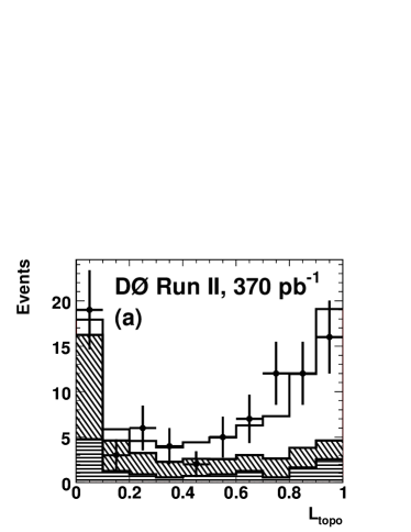
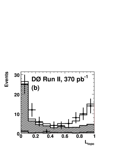
Figure 1: Distribution of the topological likelihood for the $370\,\rm pb^{-1}$ D0 Run II data sample. The distribution for $e$+jets events is shown in plot (a) and for $\mu$+jets events in plot (b). The points with error bars indicate the data, and the fitted fractions of $t\bar{t}$ events (open area), $W$+jets events (diagonally hatched), and QCD multijet events (horizontally hatched area) are superimposed.

channel	$N_{\rm evts}$	$N_{\rm top}^{\rm topo}$	$f_{\rm top}^{\rm topo}$	$f_{\rm QCD}^{\rm topo}$
$e$+jets	$\enspace 86$	$40.6~{}^{+\enspace 9.4}_{-\enspace 9.1}$	$\left(47.2\,^{+10.9}_{-10.6}\right)\%$	$\left(17.6~{}^{+\enspace 2.4}_{-\enspace 2.2}\right)\%$
$\mu$+jets	$\enspace 89$	$25.8~{}^{+\enspace 8.6}_{-\enspace 8.1}$	$\left(29.0\,^{+\enspace 9.7}_{-\enspace 9.1}\right)\%$	$\enspace\left(5.1~{}^{+\enspace 0.9}_{-\enspace 0.8}\right)\%$
$\ell$+jets	$175$	$66.4~{}^{+12.7}_{-12.2}$	$\left(37.9\,^{+\enspace 7.3}_{-\enspace 7.0}\right)\%$	$\left(11.3\pm 1.2\right)\%$

Table 2: Composition of the $e$+jets, $\mu$+jets, and $\ell$+jets data samples, estimated with the topological likelihood technique. The fractions are constrained as $f_{\rm top}^{\rm topo}+f_{W+\rm jets}^{\rm topo}+f_{\rm QCD}^{\rm topo}=1$.

The relative contributions from background events with a $W$ boson and four jets with different flavor composition are estimated using the alpgen generator. The fractions $f_{\Phi}$ of each of the six flavor configurations $\Phi=jjjj$, $b\bar{b}jj$, $c\bar{c}jj$, $(b\bar{b})jjj$, $(c\bar{c})jjj$, and $cjjj$ are listed in Table 3 bib:btagxsect . The symbol $j$ denotes a light jet not containing a charm or bottom quark, and the symbols $(b\bar{b})$ and $(c\bar{c})$ refer to situations where two heavy flavor quarks end up in the same jet. These fractions are obtained without a $b$-tagging requirement; in the $b$-tagging analysis where the event sample is divided into three classes according to the number of $b$-tagged jets per event (cf. Section VI.1), the individual numbers for each of the three separate classes are significantly different.

Contribution	$W$ + $\geq 4\ {\rm jets}$
$Wb\bar{b}jj$	$(2.72$	$\pm$	$0.11)\,\%$
$Wc\bar{c}jj$	$(4.31$	$\pm$	$0.20)\,\%$
$W(b\bar{b})jjj$	$(2.70$	$\pm$	$0.15)\,\%$
$W(c\bar{c})jjj$	$(4.69$	$\pm$	$0.36)\,\%$
$Wcjjj$	$(4.88$	$\pm$	$0.17)\,\%$
$Wjjjj$	$(80.71$	$\pm$	$0.43)\,\%$

Table 3: Fractions $f_{\Phi}$ of different flavor subprocesses contributing to the $W$+jets sample.

IV The Matrix Element Method

In this section, the measurement of the top quark mass using the Matrix Element method is described. The method is similar to the one of bib:nature ; however, the calculation of the signal probability has been revised, the normalization of the background probability is determined differently, and the method now allows a simultaneous measurement of the top quark mass and the jet energy scale bib:philipp .

An overview of the Matrix Element method is given in Section IV.1. Section IV.2 describes how $b$-tagging information is used in the analysis and discusses the parameterization of the detector response. Details on the computation of the probabilities $P_{\rm sig}$ and $P_{\rm bkg}$ are given in Sections IV.3 and IV.4.

IV.1 The Event Probability

To make maximal use of the kinematic information on the top quark mass contained in the event sample (or each individual event category in the case of the analysis using $b$-tagging information), for each selected event a probability $P_{\rm evt}$ that this event is observed is calculated as a function of the assumed top quark mass and jet energy scale. The probabilities from all events are then combined to obtain the sample probability as a function of assumed mass and jet energy scale, and the top quark mass measurement is extracted from this sample probability. To make the probability calculation tractable, simplifying assumptions in the description of the physics processes and the detector response are introduced as described in this section. Before applying it to the data, the measurement technique is calibrated using fully simulated events in the D0 detector, and the assumptions in the description of the physics processes are accounted for by systematic uncertainties.

It is assumed that the physics processes that can lead to the observed event do not interfere. The probability $P_{\rm evt}$ then in principle has to be composed from probabilities for all these processes as

$$P_{\rm evt}=\sum_{{\rm processes}\ i}f_{i}P_{i}\ ,$$ (4)

where $P_{i}$ is the probability for a given process $i$ and $f_{i}$ denotes the fraction of events from that process in the event sample. In this analysis, $P_{\rm evt}$ is composed from probabilities for two processes, $t\bar{t}$ production and $W$+jets events, as

$$P\!_{evt}\!\left(x;m_{\rm top},JES,f_{\rm top}\right)=f_{\rm top}\! \!P_{\rm sig}\!\left(x;m_{\rm top},JES\right)$$

$$+\!\left(1\!-\!f_{\rm top}\right)\! \!P_{\rm bkg}\!\left(x;JES\right)\ .$$ (5)

Here, $x$ denotes the kinematic variables of the event, $f_{\rm top}$ is the signal fraction of the event sample, and $P_{\rm sig}$ and $P_{\rm bkg}$ are the probabilities for $t\bar{t}$ and $W$+jets production, respectively. The largest background contribution is from $W$+jets events. Therefore, $P_{\rm bkg}$ is taken to be the probability for $W$+jets production. Contributions from QCD multijet events are not treated explicitly and are considered as a systematic uncertainty. The signal probability $P_{\rm sig}$ accounts for both possible flavor compositions in the hadronic $W$ decay in $\ell$+jets $t\bar{t}$ events, $W\to u\overline{d}^{\prime}$ and $W\to c\overline{s}^{\prime}$:

$$P_{\rm sig}=\frac{1}{2}\left(P_{\rm sig}^{W\to u\overline{d}^{\prime}}+P_{\rm sig}^{W\to c\overline{s}^{\prime}}\right)\ .$$ (6)

Because the event kinematics are the same, both final states are treated simultaneously in the probability calculation.

To evaluate the $t\bar{t}$ probability, all configurations of $t\bar{t}$ decay products that could have led to the observed event $x$ are considered. This includes different hadronic $W$ decays as discussed above and all possible configurations $y$ of the final state particles’ four-momenta. The probability density for given partonic final state four-momenta $y$ to be produced in the hard scattering process is proportional to the differential cross section ${\rm d}\sigma$ of the corresponding process, given by

$${\rm d}\sigma(q\bar{q}\!\to\!t\bar{t}\!\to\!y;m_{\rm top})=\frac{(2\pi)^{4}\!\left|\mathscr{M}\left(q\bar{q}\!\to\!t\bar{t}\!\to\!y\right)\right|^{2}}{q_{1}q_{2}s}{\rm d}\Phi_{6}\ .$$

The symbol $\mathscr{M}$ denotes the matrix element for the process $q\bar{q}\to t\bar{t}\to b(\ell\nu)\overline{b}(q\overline{q}^{\prime})$, $s$ is the center-of-mass energy squared, $q_{1}$ and $q_{2}$ are the momentum fractions of the colliding partons (which are assumed to be massless) within the colliding proton and antiproton, and ${\rm d}\Phi_{6}$ is an element of six-body phase space. Here the symbol $q\overline{q}^{\prime}$ stands for $u\overline{d}^{\prime}$ or $c\overline{s}^{\prime}$.

To obtain the differential cross section ${\rm d}\sigma(p\bar{p}\to t\bar{t}\to y;\,m_{\rm top})$ in $p\bar{p}$ collisions, the differential cross section from equation (IV.1) is convoluted with the parton density functions (PDF) for all possible flavor compositions of the colliding quark and antiquark,

$${\rm d}\sigma(p\bar{p}\to t\bar{t}\to y;\,m_{\rm top})$$ (8)

$$=\int\limits_{q_{1},q_{2}}\mathop{\sum_{q_{1},\,q_{2}}}_{\rm flavors} {\rm d}q_{1}{\rm d}q_{2}\ f(q_{1})\ f(q_{2})$$

$${\rm d}\sigma(q\bar{q}\to t\bar{t}\to y;\,m_{\rm top})\ ,$$

where $f(q)$ denotes the probability density to find a parton of given flavor and momentum fraction $q$ in the proton or antiproton.

The finite detector resolution is taken into account via a convolution with a transfer function $W(x,y;\,JES)$ that describes the probability to reconstruct a partonic final state $y$ as $x$ in the detector. The differential cross section to observe a given reconstructed $t\bar{t}$ event then becomes

$${\rm d}\sigma(p\bar{p}\to t\bar{t}\to x;\,m_{\rm top},JES)$$ (9)

$$=\int\limits_{y}{\rm d}\sigma(p\bar{p}\to t\bar{t}\to y;\,m_{\rm top})W(x,y;\,JES)\ .$$

Because $P_{\rm sig}$ describes $\ell$+jets $t\bar{t}$ events with both $W\to u\overline{d}^{\prime}$ and $W\to c\overline{s}^{\prime}$ decays, the transfer function depends on the quark flavors produced in the hadronic $W$ decay when $b$-tagging information is used. This is further discussed in Section IV.2.

Only events that are inside the detector acceptance and pass the trigger conditions and offline event selection are used in the measurement. The corresponding overall detector efficiency depends both on $m_{\rm top}$ and on the jet energy scale. This is taken into account in the cross section $\sigma_{\rm obs}$ of $t\bar{t}$ events observed in the detector:

$$\sigma_{\rm obs}(p\bar{p}\to t\bar{t};\,m_{\rm top},JES)$$ (10)

$$=\int\limits_{x,y}\!{\rm d}\sigma(p\bar{p}\to t\bar{t}\to y;\,m_{\rm top})W(x,y;\,JES)f_{\rm acc}(x)\ ,$$

where $f_{\rm acc}=1$ for selected events and $f_{\rm acc}=0$ otherwise.

The differential probability to observe a $t\bar{t}$ event as $x$ in the detector is then given by

$$P_{\rm sig}(x;\,m_{\rm top},JES)$$ (11)

$$=\frac{{\rm d}\sigma(p\bar{p}\to t\bar{t}\to x;\,m_{\rm top},JES)}{\sigma_{\rm obs}(p\bar{p}\to t\bar{t};\,m_{\rm top},JES)}$$

$$=\frac{1}{\sigma_{\rm obs}(p\bar{p}\to t\bar{t};\,m_{\rm top},JES)}$$

$$\quad\times\int\limits_{q_{1},q_{2},y}\mathop{\sum_{q_{1},\,q_{2}}}_{\rm flavors}{\rm d}q_{1}{\rm d}q_{2}f(q_{1})f(q_{2})$$

$$\ \quad\quad\qquad\qquad\ \frac{(2\pi)^{4}\left|\mathscr{M}(q\bar{q}\to t\bar{t}\to y)\right|^{2}}{q_{1}q_{2}s}\,{\rm d}\Phi_{6}$$

$$\ \quad\quad\qquad\qquad\ W(x,y;\,JES)\ .$$

The parametrization of the matrix element and the computation of $P_{\rm sig}$ are described in Section IV.3.

Similarly, the differential background probability is computed as

$$P_{\rm bkg}(x;\,JES)$$ (12)

$$=\frac{1}{\sigma_{\rm obs}(p\bar{p}\!\to\!W\!+\!{\rm jets};JES)}$$

$$\quad\times\!\int\limits_{q_{1},q_{2},y}\!\mathop{\sum_{q_{1},\,q_{2}}}_{\rm flavors}\!{\rm d}q_{1}{\rm d}q_{2}\,f(q_{1})\,f(q_{2})\,$$

$$\quad\quad\qquad\qquad\ \frac{(2\pi)^{4}\left|\mathscr{M}(q\bar{q}\to W\!+\!{\rm jets}\to y)\right|^{2}}{q_{1}q_{2}s}\,{\rm d}\Phi_{6}\,$$

$$\quad\quad\qquad\qquad\ W(x,y;JES)\ ,$$

where the matrix element and the total observed cross section for the process $p\bar{p}\to W+{\rm jets}$ have been used accordingly. Since the matrix element for $W$+jets production does not depend on $m_{\rm top}$, $P_{\rm bkg}$ is independent of $m_{\rm top}$; however, $P_{\rm bkg}$ in principle does depend on the jet energy scale through the transfer function. Details about the $P_{\rm bkg}$ calculation can be found in Section IV.4.

To extract the top quark mass from a set of $N$ measured events $x_{1},..,x_{N}$, a likelihood function is built from the individual event probabilities calculated according to Equation (IV.1) as

$$L(x_{1},..,x_{N};\,m_{\rm top},JES,f_{\rm top})$$ (13)

$$=\prod_{i=1}^{N}P_{\rm evt}(x_{i};\,m_{\rm top},JES,f_{\rm top})\,.$$

For every assumed pair of values $(m_{\rm top},\ JES)$, the value $f_{\rm top}^{\rm best}$ that maximizes the likelihood is determined. The top quark mass and jet energy scale are then obtained by maximizing the likelihood

$$L\left(x_{1},..,x_{N};\,m_{\rm top},JES,f_{\rm top}^{\rm best}(m_{\rm top},JES)\right)$$ (14)

$$=\prod_{i=1}^{N}P_{\rm evt}\left(x_{i};\,m_{\rm top},JES,f_{\rm top}^{\rm best}(m_{\rm top},JES)\right)$$

with respect to $m_{\rm top}$ and $JES$, taking the correlation between both parameters into account.

IV.2 Description of the Detector Response

The transfer function $W(x,y;\,JES)$ relates the characteristics $y$ of the final state partons to the measurements $x$ in the detector. The symbol $x$ denotes measurements of the jet and charged lepton energies or momenta and directions as well as $b$-tagging information for the jets. A parameterization of the detector resolution is used in the probability calculation because the full geant-based simulation would be too slow. The full simulation is however used to generate the simulated events with which the method is calibrated.

The transfer function is assumed to factorize into contributions from each measured final state particle. The angles of all measured $t\bar{t}$ decay products as well as the energy of electrons are assumed to be well-measured; in other words, the transfer functions for these quantities are given by $\delta$-distributions. This allows reducing the dimensionality of the integration over 6-particle phase space as described in Sections IV.3 and IV.4. Consequently, contributions to the integral only arise if the directions of the quark momenta in the final state agree with the measured jet directions. In addition to the energy resolution, one has to take into account the fact that the jets in the detector cannot be assigned unambiguously to a specific parton from the $t\bar{t}$ decay. Consequently, all 24 permutations of jet-quark assignments are considered.

In this section, the general form of the transfer function in the topological and $b$-tagging analyses is first discussed, followed by a description of the jet energy and muon transverse momentum resolutions.

IV.2.1 Transfer Function in the Topological Analysis

If no $b$-tagging information is used, the transfer function $W(x,y;\,JES)$ is given by

$$W(x,y;\,JES)$$

$$=W_{\mu}\left(\left(q/p_{T}\right)_{\mu}^{\rm rec},\left(q/p_{T}\right)_{\mu}^{\rm gen}\right)$$

$$\phantom{=}\times\frac{1}{24}\sum_{i=1}^{24}\delta({\rm angles})\prod_{j=1}^{4}W_{\rm jet}(E_{{\rm jet}\,j},\ E_{{\rm quark}\,k};\ JES)\ ,$$

where $W_{\mu}$ and $W_{\rm jet}$ stand for factors describing the muon transverse momentum and jet energy resolutions, respectively. The sum is over the 24 different assignments of jets $j$ to partons $k$. The factor $\delta({\rm angles})$ denotes the $\delta$ distributions that ensure that assumed and reconstructed particle directions are identical, as discussed above. For $e$+jets events, the factor for the muon transverse momentum resolution is replaced with another $\delta$-distribution. The neutrino is not measured in the detector and does not enter the transfer function. The jet transfer functions for light quark and charm jets are taken to be identical, and in the calculation of the background probability, all jets are assumed to be described by the light quark transfer function. Because the matrix elements for $W\to u\overline{d}^{\prime}$ and $W\to c\overline{s}^{\prime}$ decays are equal, and the different flavor contributions to the $W$+jets process are all parameterized by the $W$+jets matrix element without heavy flavor quarks in the final state, no distinction between different processes is necessary in the topological analysis.

IV.2.2 Transfer Function in the $b$-tagging Analysis

In the topological analysis, the information from the reconstructed jet energies determines the relative weight of different jet-parton assignments for a given partonic final state. The inclusion of $b$-tagging information allows an improved identification of the correct permutation. This additional information enters the probability calculation by weighting different permutations $i$ of jet-parton assignments with weights $w_{i}$ according to which jets, if any, are $b$-tagged. This allows to give those permutations a larger weight that assign tagged jets to $b$ quarks and untagged ones to light quarks. The transfer function is thus

$$W(x,y;\,JES)$$ (16)

$$=W_{\mu}\left(\left(q/p_{T}\right)_{\mu}^{\rm rec},\left(q/p_{T}\right)_{\mu}^{\rm gen}\right)$$

$$\phantom{=}\times\frac{\displaystyle\sum_{i=1}^{24}w_{i}\ \delta({\rm angles})\prod_{j=1}^{4}W_{\rm jet}(E_{{\rm jet}\,j},\ E_{{\rm quark}\,k};\ JES)}{\displaystyle\sum_{i=1}^{24}w_{i}}$$

(with a $\delta$-distribution instead of the factor $W_{\mu}$ in the case of $e$+jets events).

The weight $w_{i}$ for a permutation $i$ is parameterized as a product of individual weights $w_{i}(j)$ for each jet. The latter are a function of the jet flavor hypothesis $\alpha_{k}$ and the jet transverse energy $E_{T,j}$ and pseudorapidity $\eta_{j}$. For tagged jets, $w_{i}(j)$ is equal to the per-jet tagging efficiency $\epsilon_{\rm jet}(\alpha_{k};\ E_{T,j},\,\eta_{j})$ where $\alpha_{k}$ labels the three possible parton assignments to the jet: (a) $b$ quarks, (b) $c$ quarks, and (c) light quarks or gluons. For untagged jets, the $w_{i}(j)$ factors are equal to $1-\epsilon_{\rm jet}(\alpha_{k};\ E_{T,j},\,\eta_{j})$. If an event does not contain any $b$-tagged jet, all the weights $w_{i}(j)$ are set to 1.0.

To compute the signal probability of events containing $b$-tagged jets, assumptions on the jet flavors are made for the calculation of the $w_{i}$ such that hadronic $W$ decays to $u\overline{d}^{\prime}$ and $c\overline{s}^{\prime}$ final states need not be distinguished in the matrix element, allowing for a reduction of the computation time. If an event contains exactly one $b$-tagged jet, the quarks from the hadronic $W$ decay are both assumed to be light quarks ($u$, $d$, or $s$). This is justified since the tagging efficiencies for $b$ jets are much larger than those for other flavors, and there are two $b$ jets per event. For events with two or more $b$-tagged jets, a charm jet from the hadronic $W$ decay is tagged in a non-negligible fraction of cases. Consequently, the quarks from the hadronic $W$ decay are assumed to be charm quarks if the corresponding jet has been tagged, and light quarks otherwise.

The need to include jet-parton assignments with a tagged charm jet in the probability calculation can be seen by comparing the signal and background probabilities. Figure 2(a) shows the ratio of signal to background probabilities calculated in a large sample of simulated $t\bar{t}$ events with two $b$-tagged jets when only the two jet-parton assignments in which tagged jets are assigned to $b$ quarks are considered in the signal probability calculation. The hatched histogram shows the correct assignments only, whereas the open histogram shows all combinations, including the ones in which a charm quark from the $W$ decay was tagged. Figure 2(b) shows the same ratio when all combinations are included with their corresponding weight as discussed above. The tail for low signal to background probability ratios in Fig. 2(a) arises because the correct jet-parton assignment is not included in the calculation in events where one of the tagged jets comes from a charm quark. It clearly shows the need to include these assignments in the signal probability calculation.

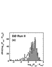
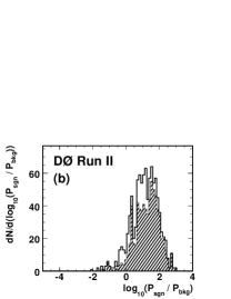
Figure 2: Monte Carlo study of the effect of charm-jet tagging on the signal to background probability ratio in the $b$-tagging analysis, for $t\bar{t}$ events generated with $m_{\rm top}=175\,\mathrm{Ge\kern-1.00006ptV}$ that contain two $b$-tagged jets. The $P_{\rm sig}$ values are calculated for the assumption $m_{\rm top}=175\,\mathrm{Ge\kern-1.00006ptV}$. (a) Only the two jet-parton assignments in which tagged jets are assigned to $b$ quarks are considered. (b) All weighted jet parton-assignments enter the probability calculation. In both plots, the hatched histogram corresponds to those cases where the two $b$-tagged jets are correctly assigned to $b$ quarks, which happens $84\%$ of the time in the double tag sample.

Because the different flavor contributions to the $W$+jets process are parameterized by the $W$+jets matrix element without heavy flavor quarks in the final state, the weights $w_{i}$ for the background probability are all equal even if $b$-tagged jets are present. Therefore, the background probability calculated for the topological analysis is used in the $b$-tagging analysis without modifications.

IV.2.3 Parameterization of the Jet Energy Resolution

The transfer function for calorimeter jets, $W_{\rm jet}(E_{j},E_{q};JES)$, yields the probability for a measurement $E_{j}$ in the detector if the true quark energy is $E_{q}$. For the case $JES=1$, it is parameterized as

$$W_{\rm jet}(E_{j},E_{q};JES\!=\!1)=\frac{1}{\sqrt{2\pi}(p_{2}+p_{3}p_{5})}\times$$ (17)

$$\Bigglb[\exp\!{\left(\!-\frac{[(E_{j}\!-\!E_{q})\!-\!p_{1}]^{2}}{2\,p_{2}^{2}}\right)}\!+\!p_{3}\exp\!{\left(\!-\frac{\![(E_{j}\!-\!E_{q})\!-\!p_{4}]^{2}}{2\,p_{5}^{2}}\!\right)}\!\Biggrb]\,.$$

The parameters $p_{i}$ are themselves functions of the quark energy, and are parameterized as linear functions of the quark energy so that

$$p_{i}=a_{i}+E_{q}\cdot b_{i}\ ,$$ (18)

with $a_{3}$ set to 0.

The parameters $a_{i}$ and $b_{i}$ are determined from simulated events, after all jet energy corrections have been applied. The parton and jet energies are fed to an unbinned likelihood fit that minimizes the $\chi^{2}$ of the fit to Equation (17) with respect to $a_{i}$ and $b_{i}$. A different set of parameters is derived for each of four $\eta$ regions: $|\eta|<0.5$, $0.5<|\eta|<1.0$, $1.0<|\eta|<1.5$, and $1.5<|\eta|<2.5$, and for three different quark varieties: light quarks ($u$, $d$, $s$, $c$), $b$ quarks with a soft muon tag in the associated jet, and all other $b$ quarks. A total of $120$ parameters describe the transfer function for all jets, and are given in Tables 4 and 5. The transfer function for light quarks in the region $|\eta|<0.5$ is shown in Fig. 3.

For $JES\neq 1$, the jet transfer function is modified as follows:

$$W_{\rm jet}(E_{j},E_{q};JES)=\frac{W_{\rm jet}(\frac{E_{j}}{JES},E_{q};1)}{JES}\ .$$ (19)

	$|\eta|$ region
par	$<0.5$		$0.5-1.0$		$1.0-1.5$		$>1.5$
$a_{1}$	$-3.00$$\times$	$10^{-1}$	$7.30$$\times$	$10^{-1}$	$4.00$$\times$	$10^{0}$	$1.01$$\times$	$10^{1}$
$b_{1}$	$-2.80$$\times$	$10^{-2}$	$-5.20$$\times$	$10^{-2}$	$-1.08$$\times$	$10^{-1}$	$-1.16$$\times$	$10^{-1}$
$a_{2}$	$3.47$$\times$	$10^{0}$	$2.05$$\times$	$10^{0}$	$2.65$$\times$	$10^{0}$	$5.54$$\times$	$10^{0}$
$b_{2}$	$9.70$$\times$	$10^{-2}$	$1.44$$\times$	$10^{-1}$	$1.51$$\times$	$10^{-1}$	$1.22$$\times$	$10^{-1}$
$a_{3}$	0.0		0.0		0.0		0.0
$b_{3}$	$3.73$$\times$	$10^{-4}$	$3.98$$\times$	$10^{-4}$	$7.74$$\times$	$10^{-4}$	$1.06$$\times$	$10^{-3}$
$a_{4}$	$1.81$$\times$	$10^{1}$	$2.23$$\times$	$10^{1}$	$1.71$$\times$	$10^{1}$	$3.77$$\times$	$10^{1}$
$b_{4}$	$-1.70$$\times$	$10^{-1}$	$-1.57$$\times$	$10^{-1}$	$3.09$$\times$	$10^{-2}$	$-1.54$$\times$	$10^{-1}$
$a_{5}$	$1.71$$\times$	$10^{1}$	$1.98$$\times$	$10^{1}$	$2.00$$\times$	$10^{1}$	$2.91$$\times$	$10^{1}$
$b_{5}$	$9.70$$\times$	$10^{-2}$	$8.04$$\times$	$10^{-2}$	$5.61$$\times$	$10^{-2}$	$-4.45$$\times$	$10^{-2}$

Table 4: Light quark transfer function parameters ($a_{i}$ in GeV).

	$|\eta|$ region
par	$<0.5$		$0.5-1.0$		$1.0-1.5$		$>1.5$
$a_{1}$	$-5.08$$\times$	$10^{0}$	$-2.38$$\times$	$10^{0}$	$0.68$$\times$	$10^{-1}$	$3.30$$\times$	$10^{0}$
$b_{1}$	$2.40$$\times$	$10^{-3}$	$-6.50$$\times$	$10^{-2}$	$-1.24$$\times$	$10^{-1}$	$-3.37$$\times$	$10^{-1}$
$a_{2}$	$3.80$$\times$	$10^{0}$	$2.40$$\times$	$10^{0}$	$9.10$$\times$	$10^{-1}$	$1.32$$\times$	$10^{1}$
$b_{2}$	$8.70$$\times$	$10^{-2}$	$1.55$$\times$	$10^{-1}$	$1.81$$\times$	$10^{-1}$	$1.32$$\times$	$10^{-1}$
$a_{3}$	0.0		0.0		0.0		0.0
$b_{3}$	$2.12$$\times$	$10^{-3}$	$3.49$$\times$	$10^{-4}$	$7.46$$\times$	$10^{-4}$	$4.06$$\times$	$10^{-2}$
$a_{4}$	$2.23$$\times$	$10^{-1}$	$2.62$$\times$	$10^{1}$	$1.17$$\times$	$10^{1}$	$-1.90$$\times$	$10^{0}$
$b_{4}$	$-1.81$$\times$	$10^{-1}$	$-4.07$$\times$	$10^{-1}$	$-7.50$$\times$	$10^{-2}$	$-5.09$$\times$	$10^{-2}$
$a_{5}$	$1.12$$\times$	$10^{1}$	$2.01$$\times$	$10^{1}$	$1.80$$\times$	$10^{1}$	$3.42$$\times$	$10^{0}$
$b_{5}$	$1.12$$\times$	$10^{-1}$	$1.22$$\times$	$10^{-1}$	$7.50$$\times$	$10^{-2}$	$1.34$$\times$	$10^{-1}$

	$|\eta|$ region
par	$<0.5$		$0.5-1.0$		$1.0-1.5$		$>1.5$
$a_{1}$	$1.10$$\times$	$10^{1}$	$4.97$$\times$	$10^{0}$	$1.29$$\times$	$10^{1}$	$1.36$$\times$	$10^{1}$
$b_{1}$	$-1.33$$\times$	$10^{-1}$	$5.30$$\times$	$10^{-3}$	$-1.65$$\times$	$10^{-1}$	$-1.32$$\times$	$10^{-1}$
$a_{2}$	$2.99$$\times$	$10^{0}$	$3.85$$\times$	$10^{0}$	$4.02$$\times$	$10^{0}$	$5.42$$\times$	$10^{0}$
$b_{2}$	$1.18$$\times$	$10^{-1}$	$4.00$$\times$	$10^{-2}$	$1.25$$\times$	$10^{-1}$	$1.18$$\times$	$10^{-1}$
$a_{3}$	0.0		0.0		0.0		0.0
$b_{3}$	$3.02$$\times$	$10^{-4}$	$1.14$$\times$	$10^{-2}$	$4.30$$\times$	$10^{-4}$	$2.42$$\times$	$10^{-4}$
$a_{4}$	$4.53$$\times$	$10^{1}$	$1.33$$\times$	$10^{1}$	$4.51$$\times$	$10^{1}$	$7.18$$\times$	$10^{1}$
$b_{4}$	$-4.54$$\times$	$10^{-1}$	$-1.91$$\times$	$10^{-1}$	$-2.15$$\times$	$10^{-1}$	$-1.24$$\times$	$10^{-1}$
$a_{5}$	$1.58$$\times$	$10^{1}$	$5.60$$\times$	$10^{0}$	$1.39$$\times$	$10^{1}$	$1.64$$\times$	$10^{1}$
$b_{5}$	$2.25$$\times$	$10^{-1}$	$1.35$$\times$	$10^{-1}$	$1.42$$\times$	$10^{-1}$	$3.40$$\times$	$10^{-2}$

Table 5: $b$ quark transfer function parameters for jets without a muon (top) and for jets containing a muon (bottom) ($a_{i}$ in GeV).

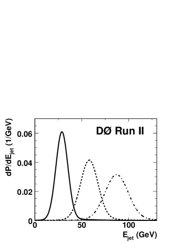
Figure 3: Jet transfer functions for light quark jets, $0.0<\left|\eta\right|<0.5$, for parton energies $E_{p}=30\,{\rm GeV}$ (solid), $60\,{\rm GeV}$ (dashed), and $90\,{\rm GeV}$ (dash-dotted curve). The parametrization corresponds to the reference jet energy scale, $JES=1.0$.

IV.2.4 Parameterization of the Muon Momentum Resolution

To describe the resolution of the central tracking chamber, the resolution of the charge divided by the transverse momentum of a particle is considered as a function of pseudorapidity. The muon transfer function is parameterized as

$$W_{\mu}\left(\left(q/p_{T}\right)_{\mu}^{\rm rec},\left(q/p_{T}\right)_{\mu}^{\rm gen}\right)$$ (20)

$$=\ \frac{1}{\sqrt{2\pi}\sigma}\,\exp\!\left[-\frac{1}{2}\left(\frac{\left(q/p_{T}\right)_{\mu}^{\rm rec}-\left(q/p_{T}\right)_{\mu}^{\rm gen}}{\sigma}\right)^{2}\right]\ ,$$

where $q$ denotes the charge and $p_{T}$ the transverse momentum of a generated (gen) muon or its reconstructed (rec) track. The resolution

$$\sigma=\left\{\begin{array}[]{cc}\sigma_{0}&{\rm for}\ |\eta|\leq\eta_{0}\vspace{2ex}\\ \sqrt{\sigma_{0}^{2}+\left[c\left(|\eta|-\eta_{0}\right)\right]^{2}}&{\rm for}\ |\eta|>\eta_{0}\end{array}\right.$$ (21)

is obtained from muon tracks in simulated events with the following values:

$$\sigma_{0} = 2.760\times 10^{-3}/{\rm GeV}$$

$$c = 5.93\times 10^{-3}/{\rm GeV}$$ (22)

$$\eta_{0} = 1.277\ .$$

The muon charge is not used in the calculation of $P_{\rm sig}$ and $P_{\rm bkg}$; however, for muons with large transverse momentum it is important to take the possibility of charge misidentification into account in the transfer function.

IV.3 Calculation of the Signal Probability $P_{\rm sig}$

The leading order matrix element for the process $q\bar{q}\to t\bar{t}$ is taken to compute $P_{\rm sig}$. Neglecting spin correlations, the matrix element is given by bib:MAHLON

$$|\mathscr{M}|^{2}=\frac{g_{s}^{4}}{9}F\overline{F}\left(2-\beta^{2}s_{qt}^{2}\right),$$ (23)

where $g_{s}^{2}/(4\pi)=\alpha_{s}$ is the strong coupling constant, $\beta$ is the velocity of the top quarks in the $t\bar{t}$ rest frame, and $s_{qt}$ denotes the sine of the angle between the incoming parton and the outgoing top quark in the $t\bar{t}$ rest frame. If the top quark decay products include the leptonically decaying $W$, while the antitop decay includes the hadronically decaying $W$, one has

$$F = \frac{g_{w}^{4}}{4}\left(\frac{m_{{b\ell\nu}}^{2}-m_{{\ell\nu}}^{2}}{\left(m_{{b\ell\nu}}^{2}-m_{t}^{2}\right)^{2}+\left(m_{t}\Gamma_{t}\right)^{2}}\right)$$ (24)

$$\times\left(\frac{m_{{b\ell\nu}}^{2}\left(1-{\hat{c}}_{b\ell}^{2}\right)+m_{{\ell\nu}}^{2}\left(1+{\hat{c}}_{b\ell}\right)^{2}}{\left(m_{{\ell\nu}}^{2}-m_{W}^{2}\right)^{2}+\left(m_{W}\Gamma_{W}\right)^{2}}\right)\ ,$$

$$\overline{F} = \frac{g_{w}^{4}}{4}\left(\frac{m_{{\overline{b}d\overline{u}}}^{2}-m_{{d\overline{u}}}^{2}}{\left(m_{{\overline{b}d\overline{u}}}^{2}-m_{t}^{2}\right)^{2}+\left(m_{t}\Gamma_{t}\right)^{2}}\right)$$ (25)

$$\times\left(\frac{m_{{\overline{b}d\overline{u}}}^{2}\left(1-{\hat{c}}_{\overline{b}d}^{2}\right)+m_{{d\overline{u}}}^{2}\left(1+{\hat{c}}_{\overline{b}d}\right)^{2}}{\left(m_{{d\overline{u}}}^{2}-m_{W}^{2}\right)^{2}+\left(m_{W}\Gamma_{W}\right)^{2}}\right)$$

(for the other case, replace $b\leftrightarrow\overline{b}$, $\ell\leftrightarrow d$, and $\nu\leftrightarrow\overline{u}$). Here, $g_{w}$ denotes the weak charge ($G_{\rm F}/\sqrt{2}=g_{w}^{2}/8m_{W}^{2}$), $m_{t}$ and $m_{W}$ are the masses of the top quark (which is to be measured) and the $W$ boson, and $\Gamma_{t}$ and $\Gamma_{W}$ are their widths. Invariant top and $W$ masses in a particular event are denoted by $m_{xyz}$ and $m_{yz}$, respectively, where $x$, $y$, and $z$ are the decay products. The cosine of the angle between particles $x$ and $y$ in the $W$ rest frame is denoted by ${\hat{c}}_{xy}$. Here and in the following, the symbols $d$ and $\overline{u}$ stand for all possible decay products in a hadronic $W$ decay. The top quark width is calculated as a function of the top quark mass according to bib:PDG .

The correct association of reconstructed jets with the final state quarks in Equations (24) and (25) is not known. Therefore, the transfer function takes into account all 24 jet-parton assignments as described in Section IV.2. However, in the case of the signal probability, the mean value of the two assignments with the 4-momenta of the quarks from the hadronic $W$ decay interchanged is computed explicitly by using the symmetrized formula

$$\overline{F} = \frac{g_{w}^{4}}{4}\left(\frac{m_{{\overline{b}d\overline{u}}}^{2}-m_{{d\overline{u}}}^{2}}{\left(m_{{\overline{b}d\overline{u}}}^{2}-m_{t}^{2}\right)^{2}+\left(m_{t}\Gamma_{t}\right)^{2}}\right)$$ (26)

$$\times\left(\frac{m_{{\overline{b}d\overline{u}}}^{2}\left(1-{\hat{c}}_{\overline{b}d}^{2}\right)+m_{{d\overline{u}}}^{2}\left(1+{\hat{c}}_{\overline{b}d}^{2}\right)}{\left(m_{{d\overline{u}}}^{2}-m_{W}^{2}\right)^{2}+\left(m_{W}\Gamma_{W}\right)^{2}}\right)$$

instead of (25), where only the terms containing ${\hat{c}}_{\overline{b}d}$ are affected. Consequently, only a summation over 12 different jet-quark assignments remains to be evaluated.

The computation of the signal probability $P_{\rm sig}$ involves an integral over the momenta of the colliding partons and over 6-body phase space to cover all possible partonic final states, cf. Equation (11). The number of dimensions of the integration is reduced by the following conditions:

• The transverse momentum of the colliding partons is assumed to be zero. Conservation of 4-momentum then implies zero transverse momentum of the $t\bar{t}$ system because the leading order matrix element is used to describe $t\bar{t}$ production. Also, the $z$ momentum and energy of the $t\bar{t}$ system are known from the momenta of the colliding partons.

• The directions of the quarks and the charged lepton in the final state are assumed to be exactly measured.

• The energy of electrons from $W$ decay is assumed to be perfectly measured. The corresponding statement is not necessarily true for high momentum muons, and an integration over the muon momentum is performed.

After these considerations, an integration over the quark momenta, the charged lepton momentum ($\mu$+jets events only), and the longitudinal component of the neutrino momentum remains to be calculated. This calculation is performed numerically with the Monte Carlo program vegas bib:VEGAS1 ; bib:VEGAS2 . The algorithm works most efficiently if the one-dimensional projections of the integrand onto the individual integration variables have well-localized peaks. The Breit-Wigner peaks of the integrand corresponding to the two top quark and two $W$ boson decays in the $t\bar{t}$ matrix element are more localized than the peaks from the jet transfer functions, suggesting that the masses are better integration variables leading to faster convergence. The computation of the parton kinematics from the integration variables must however be performed in each integration step, and this task simplifies to solving a quadratic equation when choosing $p_{z,b\nu}$ as an integration variable instead of the mass of the leptonically decaying $W$ (both solutions of the quadratic equation are considered when determining $P_{\rm sig}$). Therefore, the following integration variables are chosen for the computation of $P_{\rm sig}$:

• the magnitude $|\vec{p}_{d}|$ of the momentum of one of the quarks from the hadronic $W$ decay, with $0\leq|\vec{p}_{d}|\leq 500\ \mathrm{Ge\kern-1.00006ptV}$,

• the squared mass $m_{{d\overline{u}}}^{2}$ of the hadronically decaying $W$, $0\leq m_{{d\overline{u}}}^{2}\leq(400\ \mathrm{Ge\kern-1.00006ptV})^{2}$,

• the squared mass $m_{{\overline{b}d\overline{u}}}^{2}$ of the top quark with the hadronic $W$ decay, $0\leq m_{{\overline{b}d\overline{u}}}^{2}\leq(500\ \mathrm{Ge\kern-1.00006ptV})^{2}$,

• the squared mass $m_{{b\ell\nu}}^{2}$ of the top quark with the leptonic $W$ decay, $0\leq m_{{b\ell\nu}}^{2}\leq(500\ \mathrm{Ge\kern-1.00006ptV})^{2}$,

• the $z$ component $p_{z,b\nu}$ of the sum of the momenta of the $b$ quark and neutrino from the top quark with the leptonic $W$ decay, $-500\ \mathrm{Ge\kern-1.00006ptV}\leq p_{z,b\nu}\leq+500\ \mathrm{Ge\kern-1.00006ptV}$, and

• the muon charge divided by the muon transverse momentum (in the $\mu$+jets channel only), $-1/(100\ \mathrm{Me\kern-1.00006ptV})\leq\left(q/p_{T}\right)_{\mu}\leq+1/(100\ \mathrm{Me\kern-1.00006ptV})$.

Thus, for each point in the ($|\vec{p}_{d}|$, $m_{{d\overline{u}}}^{2}$, $m_{{\overline{b}d\overline{u}}}^{2}$, $m_{{b\ell\nu}}^{2}$, $p_{z,b\nu}$ [, $\left(q/p_{T}\right)_{\mu}$ ]) integration space the following computation is performed for each of the 12 possible jet-parton assignments (where the symmetrized form of the matrix element according to Equation (26) is used):

1. The 4-momenta of the $t\bar{t}$ decay products are calculated from the values of the integration variables, the measured jet and lepton angles, and the electron energy (in the $e$+jets case).

2. The matrix element is evaluated according to Equations (23), (24), and (26).

3. The parton distribution functions are evaluated. For consistency with the leading-order matrix element, we use the CTEQ5L bib:CTEQ5L parton distribution functions, summing over all possible quark flavors.

4. The probabilities to observe the measured jet energies and muon transverse momentum given the energies and momentum computed in the first step are evaluated using transfer functions.

5. The Jacobian determinant for the transformation from momenta in Cartesian coordinates to the ($|\vec{p}_{d}|$, $m_{{d\overline{u}}}^{2}$, $m_{{\overline{b}d\overline{u}}}^{2}$, $m_{{b\ell\nu}}^{2}$, $p_{z,b\nu}$ [, $\left(q/p_{T}\right)_{\mu}$ ]) integration space is included.

The precision of the $P_{\rm sig}$ calculation varies from typically $2\,\%$ to a maximum of $10\,\%$.

To normalize the signal probability, the integral $\int{\rm d}\sigma(p\bar{p}\to t\bar{t}\to x;\,m_{\rm top},JES)f_{\rm acc}(x)$ over 16-dimensional phase space has been computed as a function of $m_{\rm top}$ and $JES$. The detector acceptance and efficiency is taken into account as outlined in Equation (10). The results are shown in Fig. 4 for $e$+jets and $\mu$+jets events as a function of $m_{\rm top}$ for various choices of the $JES$ scale factor.

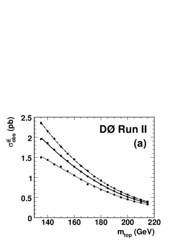
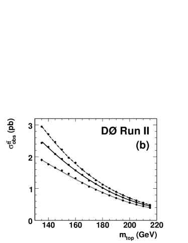
Figure 4: Observed $t\bar{t}$ cross section computed with the leading-order matrix element for (a) $e$+jets and (b) $\mu$+jets events as a function of the top quark mass $m_{\rm top}$ for different choices of the $JES$ scale factor: $JES=1.12$ (dash-dotted), $JES=1.0$ (solid), and $JES=0.88$ (dotted lines).

IV.4 Calculation of the Background Probability $P_{\rm bkg}$

To calculate $P_{\rm bkg}$, the jet directions and the charged electron or muon are taken as well-measured. The integral over the quark energies in Equation (12) is performed by generating Monte Carlo events with parton energies distributed according to the jet transfer function. In these Monte Carlo events, the neutrino transverse momentum is given by the condition that the transverse momentum of the $W$+jets system be zero, while the invariant mass of the charged lepton and neutrino is assumed to be equal to the $W$ mass to obtain the neutrino $z$ momentum (both solutions are considered). The vecbos bib:VECBOS parameterization of the matrix element is used. The mean result from all 24 possible assignments of jets to quarks in the matrix element is calculated. A minimum of 10 Monte Carlo events is generated for each measured event $x$, and the relative spread of the resulting $P_{\rm bkg}$ values is evaluated as the standard deviation divided by the mean. If the relative spread is larger than 10%, another 10 Monte Carlo events are evaluated, and this procedure is repeated until a 10% relative uncertainty is reached or a maximum of 100 Monte Carlo events has been considered.

To normalize the background probability density, $\sigma_{\rm obs}(p\bar{p}\to W+{\rm jets};\,JES)$ is chosen such that the total signal fraction $f_{\rm top}$ in the analysis without $b$ tagging is reproduced in the fit to simulated event samples containing $t\bar{t}$ and $W$+jets events. This makes use of the fact that $f_{\rm top}$ is underestimated in the fit if the background probabilities are too large and vice versa.

In the simulation, about $20-30\,\%$ of $t\bar{t}$ events have jets and partons that cannot be unambiguously matched, i.e., at least one of the four reconstructed jets cannot be matched to a parton from the $t\bar{t}$ decay within $\Delta{\cal R}<0.5$. These events yield poor top mass information and degrade the uncertainty estimate of the likelihood fit. Figure 5 illustrates that jet-parton matched $t\bar{t}$ events tend to have a higher signal than background probability density, which is how the mass fit identifies them as signal-like. There is no such separation for signal events in which one or more jets cannot be matched to a parton, so that these events contribute much less mass information to the final likelihood. This observation is consistent with the fact that a leading-order matrix element is used to describe $t\bar{t}$ events. Therefore, only jet-parton matched events are used to calibrate the $P_{\rm bkg}$ normalization. On average, the $f_{\rm top}$ fit will consequently yield the fraction of jet-parton matched (leading-order) $t\bar{t}$ events in the event sample. The quoted $f_{\rm top}$ values are corrected for this effect.

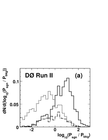
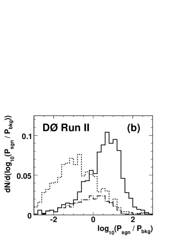
Figure 5: Distributions of $\log_{10}(P_{\rm sig}/P_{\rm bkg})$ for $t\bar{t}$ events with $m_{\rm top}=175\,\mathrm{Ge\kern-1.00006ptV}$ (solid) and $W$+jets events (dashed lines) for (a) $e$+jets events and (b) $\mu$+jets events. The $P_{\rm sig}$ values are calculated for the assumption $m_{\rm top}=175\,\mathrm{Ge\kern-1.00006ptV}$. The distributions for signal and background events are normalized individually. The distributions for those $t\bar{t}$ events that fail the requirement of jets matched to partons are shown separately (dash-dotted lines).

The $P_{\rm bkg}$ normalization is determined as follows:

• A large ensemble of simulated $t\bar{t}$ and $W$+jets events is composed with the signal fraction as determined by the topological likelihood fit described in Section III.7.

• The top mass likelihood fit described in Section V is applied to the sample and the $P_{\rm bkg}$ normalization is adjusted iteratively until the fit result yields the true signal fraction.

• The normalization of $P_{\rm bkg}$ cannot depend on the top quark mass. Therefore, the above steps are applied to $t\bar{t}$ Monte Carlo samples with different generated masses. The mean of all results is taken as the $P_{\rm bkg}$ normalization.

This procedure is applied separately for $e$+jets and $\mu$+jets events. Note that the topological likelihood discriminant is only used to determine the normalization of the background probability and the sample composition for ensemble tests used to calibrate the procedure. The topological likelihood discriminant does not otherwise enter the top quark mass fit.

V Top Quark Mass Measurement Using Topological Information

V.1 Top Quark Mass Fit

The top quark mass and overall jet energy scale $JES$ are determined as optimal values of the likelihood for the sample of selected events, which depends on the $P_{\rm sig}$ and $P_{\rm bkg}$ values. For each measured event, $P_{\rm sig}$ is calculated for various values of $m_{\rm top}$ in steps of $2.5\,\mathrm{Ge\kern-1.00006ptV}$ and various values of $JES$ in steps of $0.01$. It has been found that it is not necessary to compute the background probability for different values of the jet energy scale. Therefore, all $P_{\rm bkg}$ values are computed for $JES=1$ only. Both $P_{\rm sig}$ and $P_{\rm bkg}$ are normalized as described in Sections IV.3 and IV.4, using separate constants for $e$+jets and $\mu$+jets events. The top quark mass measurements on the $e$+jets, $\mu$+jets, and combined $\ell$+jets event samples are in each case derived from the likelihood of the event sample, given by Equation (13), in the way described below.

For given values of $m_{\rm top}$ and $JES$, each event probability $P_{\rm evt}=f_{\rm top}P_{\rm sig}+(1-f_{\rm top})P_{\rm bkg}$ depends on the signal fraction $f_{\rm top}$ of the sample, and consequently, the value of the likelihood for the event sample is a function of $f_{\rm top}$. For each ($m_{\rm top}$,$JES$) parameter pair, the best $f_{\rm top}$ parameter value is determined, and the likelihood value corresponding to this value is used in further computations. The overall result quoted for the fitted signal fraction $f_{\rm top}$ is derived from the value obtained at the point in the grid of ($m_{\rm top}$,$JES$) assumptions with the maximum likelihood value for the event sample. The uncertainty on $f_{\rm top}$ is computed by varying $f_{\rm top}$ at fixed $m_{\rm top}$ and $JES$ until $\Delta(-\ln L)=+\frac{1}{2}$. This uncertainty does not account for correlations between $f_{\rm top}$, $m_{\rm top}$, and $JES$.

The result for the top quark mass is obtained from a projection of the two-dimensional grid of likelihood values onto the $m_{\rm top}$ axis. In this projection, the correlation between $m_{\rm top}$ and the $JES$ parameter is taken into account. The probability for a given $m_{\rm top}$ hypothesis is obtained as the integral over the likelihood as a function of $JES$, using linear interpolation between the grid points and Gaussian extrapolation to account for the tails for $JES$ values outside the range considered in the grid.

The probabilities as a function of assumed top mass are converted to $-\ln L$ values. These $-\ln L$ points are then fitted with a fourth order polynomial in the region defined by the condition $\Delta\ln L<3$ around the best value. The $-\ln L$ points on either side of the $\Delta\ln L<3$ region are each fitted with a parabola, and Gaussian extrapolation is used to describe the tails outside the range of $m_{\rm top}$ hypotheses considered. The $m_{\rm top}$ value that maximizes the fitted probability is taken to be the measured value of the top quark mass. The lower and upper uncertainties on the top mass are defined such that 68% of the total probability integral is enclosed by the corresponding top mass values, with equal probabilities at both limits of the 68% confidence level region.

The same projection and fitting procedure is applied to determine the value of the $JES$ parameter.

V.2 Validation of the Method

The method is first validated using parton-level simulated $t\bar{t}$ and $W$+jets events. These have been generated with leading-order event generators (madgraph bib:MADGRAPH for $t\bar{t}$ events, alpgen for $W$+jets events), i.e., no initial or final state radiation is included. The jet energies in these events are smeared according to the transfer functions described in Section IV.2 (the treatment of the muon transverse momentum integration has been checked with additional ensemble tests not described here).

Ensembles are composed with $75$ events, $40\,\%$ of which are $t\bar{t}$ signal events. A total of $1000$ events for top masses of $160$, $170$, $175$, $180$, and $190\,\mathrm{Ge\kern-1.00006ptV}$ each are used, along with $1000$ $W$+jets events. In addition, samples with $m_{\rm top}=175\,\mathrm{Ge\kern-1.00006ptV}$ with all jet energies scaled by $0.95$ and $1.05$ are prepared in order to validate the $JES$ fit result. All events are required to pass the kinematic selection criteria listed in Table 1. The final state jets and the charged lepton must be separated according to $\Delta{\cal R}(j,j^{\prime})>0.5$ and $\Delta{\cal R}(\ell,j)>0.5$. The signal normalization is obtained according to this selection, see Section IV.3. $m_{\rm top}$ and $JES$ are obtained for each ensemble as described in Section V.1. The results of this test show that the fitted top mass and jet energy scale are unbiased within statistical uncertainties of $300\,\mathrm{Me\kern-1.00006ptV}$ and $0.003$, respectively. Furthermore, the fitted $m_{\rm top}$ value does not depend on the input $JES$ value used in the ensemble generation, and similarly, the fitted $JES$ value is independent of the true input top mass.

To test that the uncertainties obtained from the fit describe the actual measurement uncertainty, the deviation of the fitted top mass from the true value is divided by the fitted measurement uncertainty. The upper (lower) measurement uncertainty is taken if the fitted value is below (above) the true value. This definition is chosen to account for the possibility of asymmetric uncertainties. This distribution of deviations normalized by the measurement uncertainty is fitted with a Gaussian, and its width, commonly referred to as “pull width,” is in agreement with $1.0$. This is also the case for the jet energy scale measurement, for which same test has been performed.

The events used in the test outlined in this section have been generated with the same simplified model that is used in the probability calculation for the description of the production of signal and background events and the detector response, cf. Section IV. As it cannot be assumed that this simplified model correctly reproduces every aspect of the data, the method for measuring the top quark mass has been calibrated with Monte Carlo events that have been generated with the full D0 simulation. Any deviations observed in this calibration step are taken into account in the final result. The calibration is described in the following section.

V.3 Calibration of the Method

The default D0 Monte Carlo events, generated as described in Section III and passed through the full simulation of the D0 detector, are found to describe the data well. They are therefore used to derive the final calibration of the fitting procedure. $t\bar{t}$ samples with top quark masses of $160$, $170$, $175$, $180$, and $190~{}\mathrm{Ge\kern-1.00006ptV}$ and a $W$+jets sample are used. In addition, samples with $m_{\rm top}=175\,\mathrm{Ge\kern-1.00006ptV}$ where all jet energies are scaled by $0.92$, $0.96$, $1.04$, and $1.08$ are prepared in order to calibrate the $JES$ fit. For each sample and each lepton channel ($e$+jets and $\mu$+jets), $P_{\rm sig}$ and $P_{\rm bkg}$ are calculated for $1000$ events which pass the event selection. Ensembles are drawn from these event pools, with an ensemble composition as measured for the data sample. Each probability is normalized according to the flavor of the isolated lepton (see Sections IV.3 and IV.4). The QCD contribution is not added during the calibration but treated as a systematic uncertainty (cf. Section VII).

In Fig. 6, $68\%$ confidence interval distributions are shown for ensembles with $m_{\rm top}=175\,\mathrm{Ge\kern-1.00006ptV}$ and $JES=1.0$. For many pseudo-experiments, the true $m_{\rm top}$ ($JES$) value is expected to be within the fitted uncertainties in 68% of the pseudo-experiments (corresponding to a value of the conficence interval distribution of $0.68$ for this value), while other $m_{\rm top}$ ($JES$) values should be less likely to be within the uncertainties. When the error interval resulting from the integration of $68\%$ of the likelihood distribution does not include the input top mass ($JES$) value $68\%$ of the time, the uncertainty is inflated to correspond to an integration over a larger interval. The calibration results for the combined fit to the $e$+jets and $\mu$+jets ensembles are shown in Figs. 7 and 8. The fit results are corrected for the offsets $o$ and slopes $s$, and for the deviations of the pull width $w$ from 1.0 given in Table 6 to obtain the final results and their statistical uncertainties as follows:

$$m_{\rm top} = \displaystyle\frac{m_{\rm top}^{\rm fit}-o_{m_{\rm top}}-175\,\mathrm{Ge\kern-1.00006ptV}}{s_{m_{\rm top}}}+175\,\mathrm{Ge\kern-1.00006ptV}\ ,$$

$$\Delta m_{\rm top} = w_{m_{\rm top}}\left(\Delta m_{\rm top}\right)^{\rm fit}\ ,\vspace{2ex}$$

$$JES = \displaystyle\frac{JES^{\,\rm fit}-o_{JES}-1}{s_{JES}}+1\ ,\ {\rm and}$$

$$\Delta JES = w_{JES}\left(\Delta JES\right)^{\rm fit}\ .$$ (27)

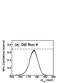
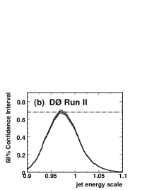
Figure 6: Calibration of the Matrix Element mass fitting procedure for the topological analysis, using ensembles with a top quark mass of 175 $\mathrm{Ge\kern-1.00006ptV}$ and $JES=1.0$. The 68% confidence interval distributions for (a) the measured top quark mass and (b) the jet energy scale is given by the solid, the upper and lower error bands by the dashed histograms. A value of 0.68 as indicated by the dash-dotted line would mean that the corresponding $m_{\rm top}$ ($JES$) value is included in the fitted $68\%$ confidence interval in 68% of the ensembles.

	offset $o$	slope $s$	pull width $w$
$m_{\rm top}$	$1.375\pm 0.085$ GeV	$1.034\pm 0.011$	$1.06\pm 0.01$
$JES$	$-0.028\pm 0.001$ GeV	$0.934\pm 0.021$	$1.09\pm 0.01$

Table 6: Calibration of the Matrix Element mass fitting procedure for the topological analysis. The offsets are quoted for a true top quark mass of $175$ GeV and a true jet energy scale of $1.0$, respectively. Only statistical uncertainties are quoted in this table.

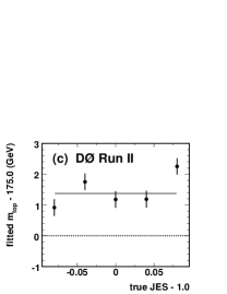
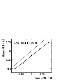
Figure 7: Calibration of the Matrix Element mass fitting procedure for the topological analysis. The upper plots show the reconstructed top mass (a) and the measured jet energy scale (b) as a function of the input top mass. The two lower plots show the reconstructed top mass (c) and the measured jet energy scale (d) as a function of the input jet energy scale. The solid lines show the results of linear fits to the points, which are used to calibrate the measurement technique. The dashed lines would be obtained for equal fitted and true values of $m_{\rm top}$ and $JES$.

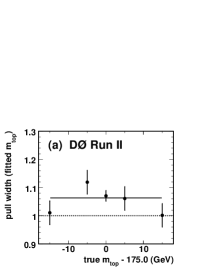
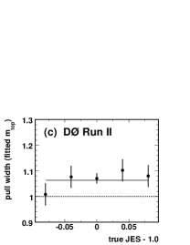
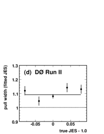
Figure 8: Calibration of the Matrix Element mass fitting procedure for the topological analysis. The upper plots show the widths of the pull distributions for the top mass (a) and jet energy scale (b) as a function of the input top mass. The two lower plots show the widths of the pull distributions for the top mass (c) and jet energy scale (d) as a function of the input jet energy scale. The solid lines show the mean pull width, while the dashed lines indicate a pull width of 1.0.

V.4 Result

The Matrix Element method is applied to the $370\,\rm pb^{-1}$ lepton+jets data set. The calibrations for $m_{\rm top}$ derived in the previous section are taken into account. The calibrated fit result for the combined lepton+jets sample is shown in Fig. 9. In this figure, the probability as a function of assumed top mass is shown together with the fitted curve (the polynomial fitted to the $-\ln L$ values as described in Section V.1 has been transformed accordingly), and the central value and 68% confidence level interval are indicated. The probability as a function of assumed $JES$ parameter is also shown. The top quark mass is measured to be

$$m_{\rm top}^{e+\rm jets} = 167.0^{\enspace+7.3}_{-10.6}\,{\rm(stat.+JES)}\,\mathrm{Ge\kern-1.00006ptV}$$

$$m_{\rm top}^{\mu+\rm jets} = 173.0^{+10.5}_{-10.9}\,{\rm(stat.+JES)}\,\mathrm{Ge\kern-1.00006ptV}$$

$$m_{\rm top}^{\ell+\rm jets} = 169.2^{\enspace+5.0}_{\enspace-7.4}\,{\rm(stat.+JES)}\,\mathrm{Ge\kern-1.00006ptV}\ .$$ (28)

The statistical uncertainties are consistent with the expectation. A comparison of the fitted uncertainties on $m_{\rm top}$ and $JES$ with the expectations from ensemble tests is given in Fig. 10. The fit yields a signal fraction $f_{\rm top}$ of $0.33\pm 0.06\,{\rm(stat.)}$, in good agreement with the result of the topological likelihood fit. The fitted jet energy scale is $JES=1.048^{+0.052}_{-0.040}\,{\rm(stat.)}$ and indicates that the data is consistent with the reference scale.

For a fixed jet energy scale, the statistical uncertainty of the fit is ${}^{+2.9}_{-3.2}\,\mathrm{Ge\kern-1.00006ptV}$; thus the component from the jet energy scale uncertainty is ${}^{+4.1}_{-6.7}\,\mathrm{Ge\kern-1.00006ptV}$. Systematic uncertainties are discussed in Section VII.

To show the likelihood as a function of both $m_{\rm top}$ and $JES$ simultaneously, the $-\ln L$ values have been fitted with a two-dimensional fourth-degree polynomial with its minimum fixed to the measurements mentioned above. The resulting contours corresponding to $\Delta\ln L=0.5$, $2.0$, $4.5$, and $8.0$ relative to the minimum are shown in Fig. 11. Note that the statistical measurement uncertainties quoted on $m_{\rm top}$ and $JES$ are obtained from the one-dimensional projections as discussed above; Fig. 11 therefore serves only illustrative purposes. Because of non-Gaussian tails, the projections of the $\Delta\ln L=0.5$ contour shown in Fig. 11 onto the $m_{\rm top}$ and $JES$ axes do not exactly correspond to these quoted statistical uncertainties.

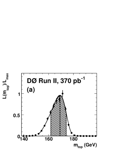
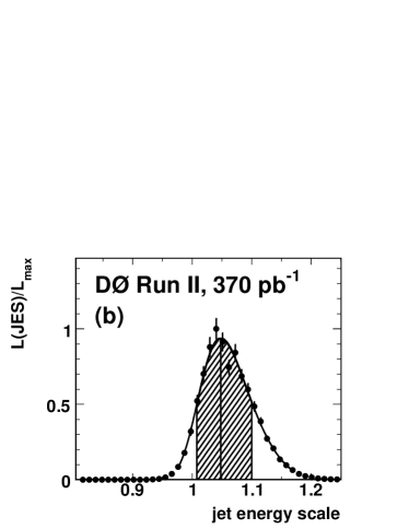
Figure 9: Application of the topological Matrix Element method to the data. The $m_{\rm top}$ and $JES$ axes correspond to the calibrated values. Plot (a) shows the probability as a function of assumed top quark mass. The correlation with the jet energy scale is taken into account. The fitted curve is shown, as well as the most likely value and the 68% confidence level region. The corresponding plot for the $JES$ parameter is shown in (b).

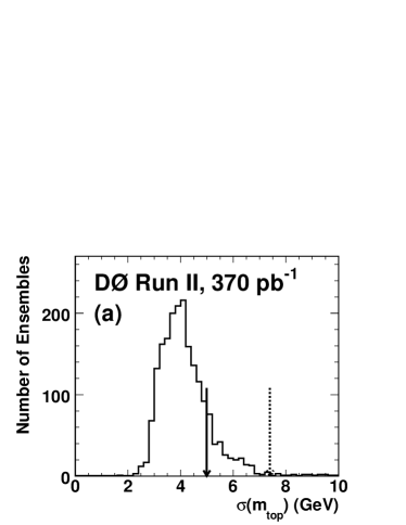
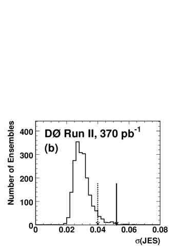
Figure 10: Uncertainties on $m_{\rm top}$ (a) and $JES$ (b) in the topological analysis. The distributions of fitted uncertainties obtained from ensemble tests are shown by the histograms. Both upper and lower uncertainties are shown; their distributions are very similar. The upper (lower) uncertainty in the data is indicated by the solid (dashed) arrow. The probability for a lower uncertainty on $m_{\rm top}$ with a magnitude larger than that observed in the data is 2%.

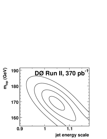
Figure 11: Application of the topological Matrix Element method to the data. Fit of a two-dimensional fourth-order polynomial to the $-\ln L$ values as a function of both $m_{\rm top}$ and $JES$. Shown are the contours corresponding to $\Delta\ln L=0.5$, $2.0$, $4.5$, and $8.0$ relative to the minimum.

VI Top Quark Mass Measurement Using $b$ Jet Identification

VI.1 Top Quark Mass Fit

The incorporation of $b$-tagging information introduces two significant modifications to the Matrix Element mass fitting technique. First, $b$-tagging information is used to determine the relative weights $w_{i}$ of the different jet-parton assignments in the signal probability calculation. The $w_{i}$ are parameterized as a function of the jet transverse energy $E_{T}$ and pseudorapidity $\eta$ and the assumed flavor $\alpha_{k}$ of the parton corresponding to the jet, as described in Section IV.2.2. The signal probability is then computed according to Equation (11). The background probability is identical to that used in the topological analysis according to Equation (12).

The second modification is to classify events into three categories according to the number of $b$-tagged jets. Each of these categories will have different signal fractions and background compositions due to the relative suppression of $W$+jets events with dominantly light quark and gluon jets. The event categories are exclusive and correspond to i) no $b$-tagged jet, ii) exactly one tagged jet, and iii) two or more tagged jets.

When the analysis is separately performed in each $n_{\rm tag}$ category, the signal fractions $f_{\rm top}^{n_{\rm tag}}$ are determined independently for each category, and $P_{\rm evt}^{n_{\rm tag}}$ is calculated as

$$P_{\rm evt}^{n_{\rm tag}}\!\left(x;\,m_{\rm top},JES,f_{\rm top}\right)=f_{\rm top}^{n_{\rm tag}}\! \!P_{\rm sig}^{n_{\rm tag}}\left(x;\,m_{\rm top},JES\right)$$

$$+(1\!-\!f_{\rm top}^{n_{\rm tag}})\! \!P_{\rm bkg}\left(x;\,JES\right)\,.$$ (29)

To combine the three categories into one analysis the three purities $f_{\rm top}^{n_{\rm tag}}$ have to be related to one inclusive signal purity $f_{\rm top}$. The purity of the $n_{\rm tag}$ sample is given by

$$f_{\rm top}^{n_{\rm tag}}=\frac{N^{n_{\rm tag}}_{\rm sig}}{N^{n_{\rm tag}}_{\rm sig}+N^{n_{\rm tag}}_{\rm bkg}}\ .$$ (30)

The numbers of signal and background events after $b$ tagging, $N^{n_{\rm tag}}_{\rm sig}$ and $N^{n_{\rm tag}}_{\rm bkg}$, can be related to the corresponding numbers for the inclusive sample, $N_{\rm sig}$ and $N_{\rm bkg}$, by

$$N^{n_{\rm tag}}_{\rm sig}=N_{\rm sig}\;\epsilon^{n_{\rm tag}}_{\rm sig}\;\;\;\text{and}\;\;\;\;N^{n_{\rm tag}}_{\rm bkg}=N_{\rm bkg}\;\epsilon^{n_{\rm tag}}_{\rm bkg}\ ,$$ (31)

where $\epsilon^{n_{\rm tag}}_{\rm sig}$ and $\epsilon^{n_{\rm tag}}_{\rm bkg}$ are the average tagging efficiencies for signal and background, respectively. They are defined as

$$\epsilon^{n_{\rm tag}}_{\rm sig} \!\!=\!\! \left\langle\frac{1}{2}\left(\epsilon^{n_{\rm tag}}_{t\overline{t}}(\{\alpha_{i}\}=bbud)+\epsilon^{n_{\rm tag}}_{t\overline{t}}(\{\alpha_{i}\}=bbcs)\right)\right\rangle\ ,$$

$$\epsilon^{n_{\rm tag}}_{\rm bkg} \!\!=\!\! \left\langle\sum_{\Phi}f_{\Phi}\epsilon^{n_{\rm tag}}_{\Phi}\right\rangle\ ,$$ (32)

with relative fractions $f_{\Phi}$ of the different flavor contributions $\Phi$ to the $W$+jets background as given in Table 3. The jets in selected QCD multijet background events have kinematic characteristics similar to those of jets in selected $W$+jets background events. Concerning the event $b$-tagging probabilities, we therefore do not distinguish between QCD multijet and $W$+jets backgrounds. The difference between multijet and $W$+jets kinematics is treated as a systematic uncertainty. The relation between $f_{\rm top}^{n_{\rm tag}}$ and the inclusive signal purity $f_{\rm top}=N_{\rm sig}/(N_{\rm sig}+N_{\rm bkg})$ is then

$$f_{\rm top}^{n_{\rm tag}}=\frac{f_{\rm top}r^{n_{\rm tag}}}{f_{\rm top}(r^{n_{\rm tag}}-1)+1}\ ,$$ (33)

where

$$r^{n_{\rm tag}}=\frac{\epsilon^{n_{\rm tag}}_{\rm sig}}{\epsilon^{n_{\rm tag}}_{\rm bkg}}\ .$$ (34)

Equation (33) needs to be corrected for the fact that the fraction of $t\bar{t}$ events that are jet-parton matched is different in each tag-multiplicity sample. Thus, a correction factor $c^{n_{\rm tag}}$ defined as the ratio of fitted $t\bar{t}$ fraction over expected $t\bar{t}$ fraction is introduced as an intercalibration of the $f_{\rm top}^{n_{\rm tag}}$ values. The top fraction for a given tag-multiplicity sample is then

$$f^{n_{\rm tag}}_{\rm top}=c^{n_{\rm tag}}\frac{f_{\rm top}r^{n_{\rm tag}}}{f_{\rm top}(r^{n_{\rm tag}}-1)+1}\ .$$ (35)

The correction factors $c^{n_{\rm tag}}$ are different for $e$+jets and $\mu$+jets events, and are given in Table 7.

	Subsample
Channel	0-tag	1-tag	$\geq 2$-tag
$e$+jets	0.68	0.86	0.94
$\mu$+jets	0.77	0.84	0.90

Table 7: Signal purity correction factors $c^{n_{\rm tag}}$.

Equation (35) defines the dependence of the signal purity on tagging multiplicity, as a function of the ratio of event-tagging efficiencies and signal purity before tagging. In order to extract the top quark mass from the total sample of selected events, the likelihoods in the individual event categories are then combined as

$$L(x_{1},..,x_{N};\,m_{\rm top},JES,f_{\rm top})$$ (36)

$$=\prod_{n_{\rm tag}=0,1,\geq 2}\prod_{i=1}^{N^{n_{\rm tag}}}P_{\rm evt}^{n_{\rm tag}}(x_{i};\,m_{\rm top},JES,f_{\rm top}^{n_{\rm tag}})\ ,$$

where $N^{n_{\rm tag}}$ is the number of events in each of the three tag-categories. As in the topological analysis, we determine the value $f_{\rm top}^{\rm best}\left(m_{\rm top},\,JES\right)$ that maximizes the likelihood $L$ in Equation (36) for each pair of assumed values of $m_{\rm top}$ and $JES$. The top quark mass and jet energy scale are then obtained by maximizing

$$\!\!\!\!\!L\left(x_{1},..,x_{N};\,m_{\rm top},JES,f_{\rm top}^{\rm best}(m_{\rm top},JES)\right)$$ (37)

$$\!\!\!\!\!=\!\!\!\!\!\!\!\!\!\prod_{n_{\rm tag}=0,1,\geq 2}\!\!\prod_{i=1}^{N^{n_{\rm tag}}}\!\!\!\!\!P_{\rm evt}^{n_{\rm tag}}\!\!\left(\!x_{i};m_{\rm top},JES,{f_{\rm top}^{\rm best}}^{n_{\rm tag}}(m_{\rm top},JES)\right)$$

as described in Section V.1 (for the 0-tag sample, the fit range is restricted to $\Delta\ln L<1$).

VI.2 Calibration of the Method

The calibration is obtained following a similar procedure as described in Section V.3. The number of events in each tag-multiplicity class is calculated by multipliying the expected number of selected events (before tagging) by the average event-tagging probability in each process:

$$N^{n_{\rm tag}}_{t\bar{t}} = N^{\rm sel}_{t\bar{t}}\epsilon^{n_{\rm tag}}_{t\bar{t}}\ {\rm and}$$

$$N^{n_{\rm tag}}_{\rm bkg} = N^{\rm sel}_{\rm bkg}\epsilon^{n_{\rm tag}}_{W+{\rm jets}}\ .$$ (38)

The $W$+jets background is classified into two categories according to the differences in event kinematics: $Wjjjj$ ($W$ + 4 jets without heavy flavor) and $Whf$ ($W$ + 4 jets including heavy flavor). Thus, the background composition for the ensemble tests after tagging is given by

$$N^{n_{\rm tag}}_{Wjjjj} = N^{\rm sel}_{\rm bkg}\ f_{Wjjjj}\ \epsilon^{n_{\rm tag}}_{Wjjjj}\ {\rm and}$$

$$N^{n_{\rm tag}}_{Whf} = N^{\rm sel}_{\rm bkg}\sum_{\Phi\neq Wjjjj}f_{\Phi}\ \epsilon^{n_{\rm tag}}_{\Phi}\ ,$$ (39)

where $f_{Wjjjj}$ is the fraction of $W+{\rm light\ jets}$, $\Phi$ denotes one of the five $W+$heavy flavor subprocesses (see Table 3), and $f_{\Phi}$ is the corresponding fraction of these subprocesses. Table 8 shows the $W$+jets composition in the 0, 1, and $\geq 2$ tag samples used in the ensemble tests. The average number of events in each tag-category and for each sample are fluctuated according to a Poisson distribution. For a given tag-category $n_{\rm tag}$, the decision of which jets are tagged is made by randomly selecting $n_{\rm tag}$ jets as tagged jets, taking into account the $E_{T}$ and $\eta$ dependence of the tagging efficiencies.

	Subsample
Contribution	0-tag	1-tag	$\geq 2$-tag
$Wjjjj$	90.9%	19.4%	0.0%
$Whf$	9.1%	80.6%	100.0%

Table 8: Background composition used in the ensemble tests for the $b$-tagging analysis. The contribution from $W$+jets events without heavy flavor is given in the first line, the contribution from events with heavy flavor jets in the second line.

In Fig. 12, $68\%$ confidence interval distributions are shown for ensembles with $m_{\rm top}=175\,\mathrm{Ge\kern-1.00006ptV}$ and $JES=1.0$. The calibration results for the combined fit are shown in Figs. 13 and 14. The final fit results are corrected for the biases and for the deviation of the pull width from 1.0 given in Table 9.

	offset $o$	slope $s$	pull width $w$
$m_{\rm top}$	$1.932\pm 0.085$ GeV	$1.018\pm 0.011$	$1.11\pm 0.01$
$JES$	$-0.028\pm 0.001$ GeV	$0.945\pm 0.021$	$1.09\pm 0.01$

Table 9: Calibration of the Matrix Element mass fitting procedure for the $b$-tagging analysis. The offsets are quoted for a true top quark mass of $175$ GeV and a true jet energy scale of $1.0$, respectively. Only statistical uncertainties are quoted in this table.

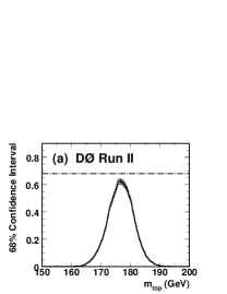
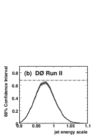
Figure 12: Calibration of the Matrix Element mass fitting procedure for the $b$-tagging analysis, using ensembles with a top quark mass of 175 $\mathrm{Ge\kern-1.00006ptV}$ and $JES=1.0$. The 68% confidence interval distributions for (a) the measured top quark mass and (b) the jet energy scale is given by the solid, the upper and lower error bands by the dashed histograms. A value of 0.68 as indicated by the dash-dotted line would mean that the corresponding $m_{\rm top}$ ($JES$) value is included in the fitted $68\%$ confidence interval in 68% of the ensembles.

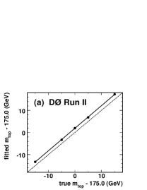
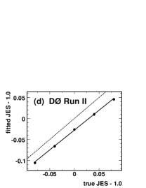
Figure 13: Calibration of the Matrix Element mass fitting procedure for the $b$-tagging analysis. The upper plots show the reconstructed top mass (a) and the measured jet energy scale (b) as a function of the input top mass. The two lower plots show the reconstructed top mass (c) and the measured jet energy scale (d) as a function of the input jet energy scale. The solid lines show the results of linear fits to the points, which are used to calibrate the measurement technique. The dashed lines would be obtained for equal fitted and true values of $m_{\rm top}$ and $JES$.

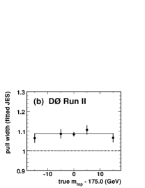
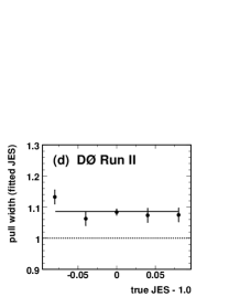
Figure 14: Calibration of the Matrix Element mass fitting procedure for the $b$-tagging analysis. The upper plots show the widths of the pull distributions for the top mass (a) and jet energy scale (b) as a function of the input top mass. The two lower plots show the widths of the pull distributions for the top mass (c) and jet energy scale (d) as a function of the input jet energy scale. The solid lines show the mean pull width, while the dashed lines indicate a pull width of 1.0.

VI.3 Result

The Matrix Element $b$-tagging method is applied to the same event sample as in Section V.4 with a calibration according to the results from Section VI.2. The probability is shown in Fig. 15 as a function of $m_{\rm top}$ and $JES$ hypothesis for each of the three tag categories. The central values and the 68% confidence level intervals are indicated in the figures. The individual results for the top quark mass are

$$m_{\rm top}^{\ell+\rm jets}({\rm 0{\text{-}}tag}) = 174.4^{+18.5}_{-12.3}\,{\rm(stat.)}\,\mathrm{Ge\kern-1.00006ptV}$$

$$m_{\rm top}^{\ell+\rm jets}({\rm 1{\text{-}}tag}) = 173.1^{\enspace+5.1}_{\enspace-5.2}\,{\rm(stat.)}\,\mathrm{Ge\kern-1.00006ptV}$$

$$m_{\rm top}^{\ell+\rm jets}({\rm 2{\text{-}}tag}) = 163.2^{\enspace+6.8}_{\enspace-6.2}\,{\rm(stat.)}\,\mathrm{Ge\kern-1.00006ptV}$$ (40)

in the 0-tag, 1-tag, and $\geq 2$-tag categories. The corresponding results for the jet energy scale are $JES(0$-${\rm tag})=0.986^{+0.084}_{-0.091}\,{\rm(stat.)}$, $JES(1$-${\rm tag})=1.011^{+0.049}_{-0.045}\,{\rm(stat.)}$, and $JES(2$-${\rm tag})=1.094^{+0.071}_{-0.066}\,{\rm(stat.)}$, respectively.

The result for the combined event sample is

$$m_{\rm top}^{e+\rm jets} = 170.1^{+4.6}_{-6.3}\,{\rm(stat.+JES)}\,\mathrm{Ge\kern-1.00006ptV}$$

$$m_{\rm top}^{\mu+\rm jets} = 172.6^{+9.4}_{-8.6}\,{\rm(stat.+JES)}\,\mathrm{Ge\kern-1.00006ptV}$$

$$m_{\rm top}^{\ell+\rm jets} = 170.3^{+4.1}_{-4.5}\,{\rm(stat.+JES)}\,\mathrm{Ge\kern-1.00006ptV};$$ (41)

the $\ell$+jets measurement is shown in Fig. 16. The statistical uncertainties are consistent with the expectation. Figure 17 shows the distributions of the expected $m_{\rm top}$ uncertainty compared to the observed result. The fit yields a signal fraction $f_{\rm top}$ of $0.31\pm 0.09\,{\rm(stat.)}$, in good agreement with the result of the topological likelihood fit. The fitted jet energy scale is $JES=1.027^{+0.035}_{-0.032}\,{\rm(stat.)}$ and indicates that the data is consistent with the reference scale.

For a fixed jet energy scale, the statistical uncertainty of the fit is $\pm 2.5\,\mathrm{Ge\kern-1.00006ptV}$; thus the component from the jet energy scale uncertainty is ${}^{+3.2}_{-3.7}\,\mathrm{Ge\kern-1.00006ptV}$. Systematic uncertainties are discussed in Section VII.

To show the likelihood as a function of both $m_{\rm top}$ and $JES$ simultaneously, the $-\ln L$ values have been fitted with a two-dimensional fourth-degree polynomial with its minimum fixed to the measurements mentioned above. The resulting contours corresponding to $\Delta\ln L=0.5$, $2.0$, $4.5$, and $8.0$ relative to the minimum are shown in Fig. 18. Note that because of non-Gaussian tails, the projections of the $\Delta\ln L=0.5$ contour onto the $m_{\rm top}$ and $JES$ axes do not exactly correspond to the 68% confidence intervals around the most likely values; Fig. 18 therefore serves only illustrative purposes.

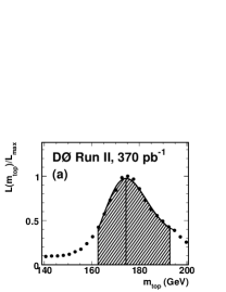
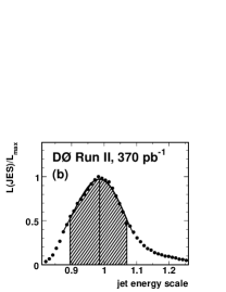
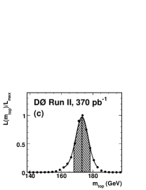
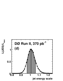
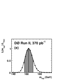
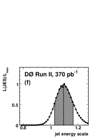
Figure 15: Application of the Matrix Element $b$-tagging method to the data. The fitted $m_{\rm top}$ and $JES$ likelihoods for each of the 3 tag-categories: 0-tag ((a) and (b)), 1-tag ((c) and (d)), and $\geq 2$-tag ((e) and (f)). The 68% confidence-level interval around the most likely value is shown by the hatched region under the fitted curve.

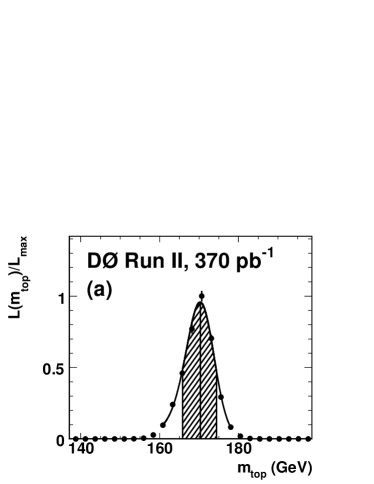
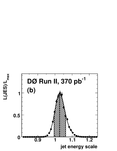
Figure 16: Application of the Matrix Element $b$-tagging method to the data. The final results of the fitted $m_{\rm top}$ (a) and $JES$ (b) likelihoods for the combined event sample are shown. The 68% confidence-level interval around the most likely value is indicated by the hatched region under the fitted curve.

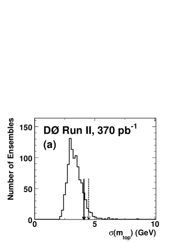
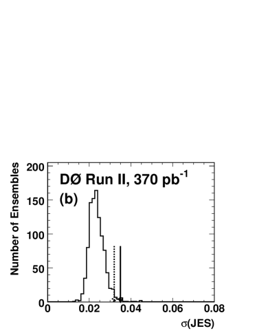
Figure 17: Uncertainties on $m_{\rm top}$ (a) and $JES$ (b) obtained in the $b$-tagging analysis with the combined sample. The distributions of fitted uncertainties obtained from ensemble tests are shown by the histograms. Both upper and lower uncertainties are shown; their distributions are very similar. The upper (lower) uncertainty in the data is indicated by the solid (dashed) arrow.

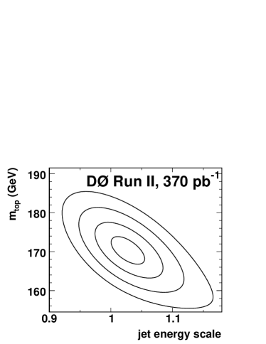
Figure 18: Application of the Matrix Element $b$-tagging method to the data. Fit of a two-dimensional fourth-order polynomial to the $-\ln L$ values as a function of both $m_{\rm top}$ and $JES$. Shown are the contours corresponding to $\Delta\ln L=0.5$, $2.0$, $4.5$, and $8.0$ relative to the minimum.

VII Systematic Uncertainties

Systematic uncertainties arise from three sources: modeling of the physics processes for $t\bar{t}$ production and background, modeling of the detector performance, and uncertainties in the methods themselves. Table 10 lists all uncertainties. The jet energy scale uncertainty is included in the statistical uncertainty. The total systematic uncertainty on the top mass measurement is obtained by adding all contributions in quadrature. In general, to evaluate systematic uncertainties, the simulation of events used to calibrate the measurement has been varied, while the measurement method itself has been kept unchanged.

Source of Uncertainty	Topological Analysis	$b$-Tagging Analysis
Statistical uncertainty and jet energy scale	$+5.0~{}-7.4$	$+4.1~{}-4.5$
Physics modeling:
Signal modeling	$\pm 0.34$	$\pm 0.46$
Background modeling	$\pm 0.32$	$\pm 0.40$
PDF uncertainty	$+0.26~{}-0.40$	$+0.16~{}-0.39$
$b$ fragmentation	$\pm 0.71$	$\pm 0.56$
$b$/$c$ semileptonic decays	$+0.06~{}-0.07$	$\pm 0.05$
Detector modeling:
$JES$ $p_{T}$ dependence	$\pm 0.25$	$\pm 0.19$
$b$ response (h/e)	$+0.87~{}-0.75$	$+0.63~{}-1.43$
Trigger	$\pm 0.08$	$+0.08~{}-0.13$
$b$ tagging	–	$\pm 0.24$
Method:
Signal fraction	$+0.50~{}-0.17$	$\pm 0.15$
QCD contamination	$\pm 0.67$	$\pm 0.29$
MC calibration	$\pm 0.17$	$\pm 0.48$
Total systematic uncertainty	$+1.5~{}-1.4$	$+1.2~{}-1.8$
Total uncertainty	$+5.2~{}-7.5$	$+4.3~{}-4.9$

Table 10: Summary of uncertainties on the top quark mass. All values are quoted in GeV.

VII.1 Physics Modeling

• Signal modeling: When $t\bar{t}$ events are produced in association with a jet, the additional jet can be misinterpreted as a product of the $t\bar{t}$ decay. Also, the $t\bar{t}$ system may then have significant transverse momentum, in contrast to the assumption made in the calculation of $P_{\rm sig}$. In spite of the event selection that requires exactly four jets, these events can be selected if one of the jets from the $t\bar{t}$ decay is not reconstructed.

  Such events are present in the simulated events used for the calibration of the method. To assess the uncertainty in the modeling of these effects, events have been generated using a dedicated simulation of the production of $t\bar{t}$ events together with an additional parton. The fraction of such events is estimated to be no larger than 30% (according to the difference between cross section calculations in leading and next-to-leading order).

  Two large ensembles of simulated events are composed according to the sample composition in the data, one using only events with an additional parton for the signal, and the second with the default simulation. The result obtained with the default calibration is quoted as central value. A systematic uncertainty of $30\%$ of the difference in top mass results between these two ensembles is quoted.

  In addition, simulated $gg\to t\bar{t}$ and $q\bar{q}\to t\bar{t}$ events have been compared. The top mass calibration has been rederived using only $gg\to t\bar{t}$ or $q\bar{q}\to t\bar{t}$ events to simulate the signal, and no significant difference has been found. Thus no additional uncertainty on the result is assigned.

• Background modeling: In order to study the sensitivity of the measurement to the choice of background model, the standard $W$+jets Monte Carlo sample is replaced by an alternative sample with the default factorization scale of $Q^{2}=m_{W}^{2}+\sum_{j}p_{T,j}^{2}$ replaced by $Q^{\prime 2}=\left<p_{T,j}\right>^{2}$. One large ensemble of events is composed using both the default and the alternative background model. The difference of results obtained with these ensembles is symmetrized and is assigned as a systematic uncertainty.

• PDF uncertainty: Leading-order matrix elements are used to calculate both $P_{\rm sig}$ and $P_{\rm bkg}$. Consequently, both calculations use a leading order parton distribution function (PDF): CTEQ5L bib:CTEQ5L . To study the systematic uncertainty on $m_{\rm top}$ due to this choice, the variations provided with the next-to-leading-order PDF set CTEQ6M bib:CTEQ6Mvar are used, and the result obtained with each of these variations is compared with the result using the default CTEQ6M parametrization. The difference between the results obtained with the CTEQ5L and MRST leading order PDF sets is taken as another uncertainty. Finally, the effect of a variation of $\alpha_{s}$ is evaluated. In all cases, a large ensemble has been composed of events simulated with CTEQ5L, and these have been reweighted such that distributions according to the desired PDF set are obtained. The individual systematic uncertainties are added in quadrature. The systematic uncertainty is dominated by that from the variation of CTEQ6M parameters.

• $b$ fragmentation: While the overall jet energy scale uncertainty is included in the statistical uncertainty from the fit, differences in the $b$/light jet energy scale ratio between data and simulation may still affect the measurement. Possible effects from such differences are studied using simulated $t\bar{t}$ events with different fragmentation models for $b$ jets. The default Bowler bib:BOWLER scheme with $r_{b}=1.0$ is replaced with $r_{b}=0.69$ or with Peterson bib:PETERSON fragmentation with $\epsilon_{b}=0.00191$. Simulation studies show that the variation of $r_{b}$ results in a change of the mean scaled energy $\langle x_{B}\rangle$ of $b$ hadrons that is larger than the uncertainties reported in bib:bfragLEP , while the uncertainty on the shape of the $x_{B}$ distribution is taken into account by the comparison of the Bowler and Peterson schemes. One large ensemble is built using events from each of the three simulations. The absolute values of the deviations of top mass results from the standard sample are added in quadrature and symmetrized.

• $b/c$ semileptonic decays: The reconstructed energy of $b$ jets containing a semileptonic bottom or charm decay is in general lower than that of jets containing only hadronic decays. This can only be taken into account for jets in which a soft muon is reconstructed. Thus, the fitted top quark mass still depends on the semileptonic $b$ and $c$ decay branching ratios. They have been varied by reweighting events in one large ensemble of simulated events within the bounds given in bib:PDG .

VII.2 Detector Modeling

• $JES$ $p_{T}$ and $|\eta|$ dependence: The relative difference between the jet energy scales in data and Monte Carlo is fitted with a global scale factor, and the corresponding uncertainty is included in the quoted (stat. + JES) uncertainty. Any discrepancy between data and simulation other than a global scale difference may lead to an additional uncertainty on the top quark mass. To estimate this uncertainty, the energies of jets in the events of one large ensemble have been scaled by a factor of $(1+0.02\frac{E_{\rm jet}}{100\,{\rm GeV}})$ where $E_{\rm jet}$ is the default jet energy. The value $0.02$ is suggested by studies of $\gamma$+jets events. The top mass result from the modified ensemble has been compared to the default number, and the symmetrized difference is taken as a systematic uncertainty.

  Similarly, to estimate the effect of a possible $|\eta|$ dependence of the jet energy scale ratio between data and simulation, the jet energies have also been scaled by a factor $(1-0.01|\eta|)$ as suggested by $\gamma$+jets events. No significant effect on the top quark mass has been observed and thus no additional systematic uncertainty is assigned.

• Relative $b$/light jet energy scale: Variations of the h/e calorimeter response lead to differences in the $b$/light jet energy scale ratio between data and simulation in addition to the variations of the $b$ fragmentation function considered in Section VII.1. This uncertainty has been evaluated by scaling the energies of $b$ jets in one large ensemble and studying the effect on the top quark mass.

• Trigger: The trigger efficiencies used in composing ensembles for the calibration of the measurement are varied by their uncertainties, and the uncertainties from all variations are summed in quadrature.

• $b$ tagging: The $b$-tagging efficiencies are varied within the uncertainties as determined from the data, and the variations are propagated to the final result.

Note that no systematic uncertainty is quoted due to multiple interactions/uranium noise as opposed to the Run I measurement. The effect is much smaller in Run II as a consequence of the reduced integration time in the calorimeter readout. It is moreover covered by the jet energy scale uncertainty, as the offset correction is computed seperately for data and Monte Carlo in Run II, accounting for effects arising from electronic noise and pileup.

VII.3 Method

• Signal fraction: The normalization procedure of the background probability described in Section IV.4 is chosen such that the signal fraction $f_{\rm top}$ as measured with the topological likelihood fit and given in Table 2 is reproduced. However, the signal fraction is slightly overestimated for low true signal fractions, which leads to a small bias in the resulting top mass. The signal fraction in ensemble tests used for the calibration is varied within the uncertainties determined from the topological likelihood fit, and the resulting variation of the top quark mass is taken as a systematic uncertainty.

• QCD background: The $W$+jets simulation is used to model the small QCD background in the selected event sample in the analysis. The systematic uncertainty from this assumption is computed by selecting a dedicated QCD-enriched sample of events from data by inverting the lepton isolation cut in the event selection. The calibration of the method is repeated with ensembles formed where these events are used to model the QCD background events whose fraction is given in Table 2. The resulting change is assigned as a systematic uncertainty.

• MC calibration: The calibration of the top mass measurement is varied according to the statistical uncertainty of the calibration curves shown in Figs. 7 and 13.

VIII Summary

A measurement of the top quark mass using lepton+jets $t\bar{t}$ events in 370 $\rm pb^{-1}$ of data collected with the D0 detector at Run II of the Fermilab Tevatron Collider has been presented. The events are analysed with the Matrix Element method, which is designed to make maximal use of the kinematic information in the selected events. To avoid a large systematic uncertainty, an overall scale factor $JES$ for the energy of calorimeter jets is determined simultaneously with the top quark mass. This in-situ calibration of the jet energy scale helps reduce the overall uncertainty on the top quark mass when combining with other measurements.

The resulting top quark mass is

$$m_{\rm top}=169.2^{+5.0}_{-7.4}\,{\rm(stat.+JES)}\,^{+1.5}_{-1.4}\,{\rm(syst.)}\,\mathrm{Ge\kern-1.00006ptV}$$ (42)

for an analysis that uses only topological information, and

$$m_{\rm top}=170.3^{+4.1}_{-4.5}\,{\rm(stat.+JES)}\,^{+1.2}_{-1.8}\,{\rm(syst.)}\,\mathrm{Ge\kern-1.00006ptV}$$ (43)

when $b$-tagging information is included. The jet energy scale is $JES=1.048^{+0.052}_{-0.040}\,{\rm(stat.)}$ in the topological analysis and $JES=1.027^{+0.035}_{-0.032}\,{\rm(stat.)}$ when $b$ tagging is included, indicating consistency with the reference scale. The two results are consistent with each other. To obtain a value for the top quark mass in combination with other measurements, the second, more precise value should be used.

References

- (1) The ALEPH, DELPHI, L3, OPAL, and SLD Collaborations, the LEP Electroweak Working Group, SLD Electroweak Group, and SLD Heavy Flavour Group, Phys. Rept. 427, 257 (2006).
-
(2)
F. Abe et al.,
Phys. Rev. Lett. 74, 2626 (1995);
S. Abachi et al., Phys. Rev. Lett. 74, 2632 (1995). -
(3)
F. Abe et al.,
Phys. Rev. Lett. 80, 2767 (1998);
F. Abe et al., Phys. Rev. Lett. 80, 2779 (1998);
F. Abe et al., Phys. Rev. Lett. 82, 271 (1999);
F. Affolder et al., Phys. Rev. D 63, 032003 (2001);
S. Abachi et al., Phys. Rev. Lett. 79, 1197 (1997);
B. Abbott et al., Phys. Rev. Lett. 80, 2063 (1998);
B. Abbott et al., Phys. Rev. D 58, 052001 (1998);
B. Abbott et al., Phys. Rev. D 60, 052001 (1999);
V. M. Abazov et al., Nature 429, 638 (2004);
V. M. Abazov et al. Phys. Lett. B 606, 25 (2005). -
(4)
A. Abulencia et al.,
Phys. Rev. D 73, 032003 (2006);
A. Abulencia et al., Phys. Rev. Lett. 96, 022004 (2006). - (5) V. M. Abazov et al., Nature 429, 638 (2004).
- (6) P. Schieferdecker, FERMILAB-THESIS 2005-46.
- (7) V. M. Abazov et al., Nucl. Instrum. Methods A 565, 463 (2006).
- (8) S. Abachi et al., Nucl. Instrum. Methods Phys. Res. A 338, 185 (1994).
- (9) V. M. Abazov et al., physics/0503151 (2005).
- (10) V. M. Abazov et al., Phys. Lett. B 626, 35 (2005).
- (11) M. L. Mangano et al., JHEP 307, 1 (2003).
- (12) T. Sjöstrand, P. Edén, C. Friberg, L. Lönnblad, G. Miu, S. Mrenna, and E. Norrbin, Computer Phys. Commun. 135, 238 (2001).
- (13) V. M. Abazov et al., Phys. Lett. B 626, 45 (2005).
- (14) G. Mahlon and S. J. Parke, Phys. Lett. B 411, 173 (1997).
- (15) W.-M. Yao et al. J. Phys. G 33, 1 (2006).
- (16) G. P. Lepage, Journal of Computational Physics 27, 192 (1978).
- (17) G. P. Lepage, Cornell preprint CLNS:80-447, (1980).
- (18) H. L. Lai et al., Eur. Phys. J. C 12, 375 (2000).
- (19) F. A. Berends, H. Kuijf, B. Tausk, and W. T. Giele, Nucl. Phys. B357, 32 (1991).
- (20) F. Maltoni, T. Stelzer, JHEP 302, 27 (2003).
- (21) J. Pumplin et al., JHEP 0207, 012 (2002).
- (22) M. G. Bowler, Z. Phys C 11, 169 (1981).
- (23) C. Peterson et. al, Phys. Rev. D 27, 105 (1983).
-
(24)
K. Abe et. al,
Phys. Rev. Lett. 84, 4300 (2000);
A. Heister et. al, Phys. Lett. B 512, 30 (2001);
G. Abbiendi et. al, Eur. Phys. J. C 29, 463 (2003). - (25) On leave from IEP SAS Košice, Slovakia.
- (26) Visitor from Helsinki Institute of Physics, Helsinki, Finland.