EUROPEAN ORGANISATION FOR NUCLEAR RESEARCH (CERN)

CERN-EP/2006-xxx

26 September 2006

Fermion pair production in ${\mathrm{e^{+}e^{-}}}$ collisions at 189-209 GeV and constraints on physics beyond the Standard Model

The ALEPH Collaboration${}^{*})$

Cross sections, angular distributions and forward-backward asymmetries are presented, of two-fermion events produced in ${\mathrm{e}}^{+}{\mathrm{e}}^{-}$collisions at centre-of-mass energies from 189 to 209 GeV at LEP, measured with the ALEPH detector. Results for ${\mathrm{e}}^{+}{\mathrm{e}}^{-}$, ${\mathrm{\mu^{+}\mu^{-}}}$, ${\mathrm{\tau^{+}\tau^{-}}}$, ${\mathrm{q}}\bar{\mathrm{q}}$, $\mathrm{b}\bar{\mathrm{b}}$ and ${\mathrm{c}}\bar{\mathrm{c}}$ production are in agreement with the Standard Model predictions. Constraints are set on scenarios of new physics such as four-fermion contact interactions, leptoquarks, Z bosons, TeV-scale quantum gravity and R-parity violating squarks and sneutrinos.

To be published in The European Physical Journal C

Dedicated to the memory of John Strong who died on July 31, 2006

——————————————– ${}^{*})$ See next pages for the list of authors

The ALEPH Collaboration

S. Schael

Physikalisches Institut der RWTH-Aachen, D-52056 Aachen, Germany

R. Barate, R. Brunelière, I. De Bonis, D. Decamp, C. Goy, S. Jézéquel, J.-P. Lees, F. Martin, E. Merle, M.-N. Minard, B. Pietrzyk, B. Trocmé

Laboratoire de Physique des Particules (LAPP), IN2P3-CNRS, F-74019 Annecy-le-Vieux Cedex, France

S. Bravo, M.P. Casado, M. Chmeissani, J.M. Crespo, E. Fernandez, M. Fernandez-Bosman, Ll. Garrido,15 M. Martinez, A. Pacheco, H. Ruiz

Institut de Física d’Altes Energies, Universitat Autònoma de Barcelona, E-08193 Bellaterra (Barcelona), Spain7

A. Colaleo, D. Creanza, N. De Filippis, M. de Palma, G. Iaselli, G. Maggi, M. Maggi, S. Nuzzo, A. Ranieri, G. Raso,24 F. Ruggieri, G. Selvaggi, L. Silvestris, P. Tempesta, A. Tricomi,3 G. Zito

Dipartimento di Fisica, INFN Sezione di Bari, I-70126 Bari, Italy

X. Huang, J. Lin, Q. Ouyang, T. Wang, Y. Xie, R. Xu, S. Xue, J. Zhang, L. Zhang, W. Zhao

Institute of High Energy Physics, Academia Sinica, Beijing, The People’s Republic of China8

D. Abbaneo, T. Barklow,26 O. Buchmüller,26 M. Cattaneo, B. Clerbaux,23 H. Drevermann, R.W. Forty, M. Frank, F. Gianotti, J.B. Hansen, J. Harvey, D.E. Hutchcroft,30, P. Janot, B. Jost, M. Kado,2 P. Mato, A. Moutoussi, F. Ranjard, L. Rolandi, D. Schlatter, F. Teubert, A. Valassi, I. Videau

European Laboratory for Particle Physics (CERN), CH-1211 Geneva 23, Switzerland

F. Badaud, S. Dessagne, A. Falvard,20 D. Fayolle, P. Gay, J. Jousset, B. Michel, S. Monteil, D. Pallin, J.M. Pascolo, P. Perret

Laboratoire de Physique Corpusculaire, Université Blaise Pascal, IN2P3-CNRS, Clermont-Ferrand, F-63177 Aubière, France

J.D. Hansen, J.R. Hansen, P.H. Hansen, A.C. Kraan, B.S. Nilsson

Niels Bohr Institute, 2100 Copenhagen, DK-Denmark9

A. Kyriakis, C. Markou, E. Simopoulou, A. Vayaki, K. Zachariadou

Nuclear Research Center Demokritos (NRCD), GR-15310 Attiki, Greece

A. Blondel,12 J.-C. Brient, F. Machefert, A. Rougé, H. Videau

Laoratoire Leprince-Ringuet, Ecole Polytechnique, IN2P3-CNRS, F-91128 Palaiseau Cedex, France

V. Ciulli, E. Focardi, G. Parrini

Dipartimento di Fisica, Università di Firenze, INFN Sezione di Firenze, I-50125 Firenze, Italy

A. Antonelli, M. Antonelli, G. Bencivenni, F. Bossi, G. Capon, F. Cerutti, V. Chiarella, P. Laurelli, G. Mannocchi,5 G.P. Murtas, L. Passalacqua

Laboratori Nazionali dell’INFN (LNF-INFN), I-00044 Frascati, Italy

J. Kennedy, J.G. Lynch, P. Negus, V. O’Shea, A.S. Thompson

Department of Physics and Astronomy, University of Glasgow, Glasgow G12 8QQ,United Kingdom10

S. Wasserbaech

Utah Valley State College, Orem, UT 84058, U.S.A.

R. Cavanaugh,4 S. Dhamotharan,21 C. Geweniger, P. Hanke, V. Hepp, E.E. Kluge, A. Putzer, H. Stenzel, K. Tittel, M. Wunsch19

Kirchhoff-Institut für Physik, Universität Heidelberg, D-69120 Heidelberg, Germany16

R. Beuselinck, W. Cameron, G. Davies, P.J. Dornan, M. Girone,1 R.D. Hill, N. Marinelli, J. Nowell, S.A. Rutherford, J.K. Sedgbeer, J.C. Thompson,14 R. White

Department of Physics, Imperial College, London SW7 2BZ, United Kingdom10

V.M. Ghete, P. Girtler, E. Kneringer, D. Kuhn, G. Rudolph

Institut für Experimentalphysik, Universität Innsbruck, A-6020 Innsbruck, Austria18

E. Bouhova-Thacker, C.K. Bowdery, D.P. Clarke, G. Ellis, A.J. Finch, F. Foster, G. Hughes, R.W.L. Jones, M.R. Pearson, N.A. Robertson, M. Smizanska

Department of Physics, University of Lancaster, Lancaster LA1 4YB, United Kingdom10

O. van der Aa, C. Delaere,28 G.Leibenguth,31 V. Lemaitre29

Institut de Physique Nucléaire, Département de Physique, Université Catholique de Louvain, 1348 Louvain-la-Neuve, Belgium

U. Blumenschein, F. Hölldorfer, K. Jakobs, F. Kayser, A.-S. Müller, G. Quast32 B. Renk, H.-G. Sander, S. Schmeling, H. Wachsmuth, C. Zeitnitz, T. Ziegler

Institut für Physik, Universität Mainz, D-55099 Mainz, Germany16

A. Bonissent, P. Coyle, C. Curtil, A. Ealet, D. Fouchez, P. Payre, A. Tilquin

Centre de Physique des Particules de Marseille, Univ Méditerranée, IN2P3-CNRS, F-13288 Marseille, France

F. Ragusa

Dipartimento di Fisica, Università di Milano e INFN Sezione di Milano, I-20133 Milano, Italy.

A. David, H. Dietl,33 G. Ganis,27 K. Hüttmann, G. Lütjens, W. Männer33, H.-G. Moser, R. Settles, M. Villegas, G. Wolf

Max-Planck-Institut für Physik, Werner-Heisenberg-Institut, D-80805 München, Germany161616Supported by Bundesministerium für Bildung und Forschung, Germany.

J. Boucrot, O. Callot, M. Davier, L. Duflot, J.-F. Grivaz, Ph. Heusse, A. Jacholkowska,6 L. Serin, J.-J. Veillet

Laboratoire de l’Accélérateur Linéaire, Université de Paris-Sud, IN2P3-CNRS, F-91898 Orsay Cedex, France

P. Azzurri, G. Bagliesi, T. Boccali, L. Foà, A. Giammanco, A. Giassi, F. Ligabue, A. Messineo, F. Palla, G. Sanguinetti, A. Sciabà, G. Sguazzoni, P. Spagnolo, R. Tenchini, A. Venturi, P.G. Verdini

Dipartimento di Fisica dell’Università, INFN Sezione di Pisa, e Scuola Normale Superiore, I-56010 Pisa, Italy

O. Awunor, G.A. Blair, G. Cowan, A. Garcia-Bellido, M.G. Green, T. Medcalf,25 A. Misiejuk, J.A. Strong,25 P. Teixeira-Dias

Department of Physics, Royal Holloway & Bedford New College, University of London, Egham, Surrey TW20 OEX, United Kingdom10

R.W. Clifft, T.R. Edgecock, P.R. Norton, I.R. Tomalin, J.J. Ward

Particle Physics Dept., Rutherford Appleton Laboratory, Chilton, Didcot, Oxon OX11 OQX, United Kingdom10

B. Bloch-Devaux, D. Boumediene, P. Colas, B. Fabbro, E. Lançon, M.-C. Lemaire, E. Locci, P. Perez, J. Rander, B. Tuchming, B. Vallage

CEA, DAPNIA/Service de Physique des Particules, CE-Saclay, F-91191 Gif-sur-Yvette Cedex, France17

A.M. Litke, G. Taylor

Institute for Particle Physics, University of California at Santa Cruz, Santa Cruz, CA 95064, USA22

C.N. Booth, S. Cartwright, F. Combley,25 P.N. Hodgson, M. Lehto, L.F. Thompson

Department of Physics, University of Sheffield, Sheffield S3 7RH, United Kingdom10

A. Böhrer, S. Brandt, C. Grupen, J. Hess, A. Ngac, G. Prange

Fachbereich Physik, Universität Siegen, D-57068 Siegen, Germany16

C. Borean, G. Giannini

Dipartimento di Fisica, Università di Trieste e INFN Sezione di Trieste, I-34127 Trieste, Italy

H. He, J. Putz, J. Rothberg

Experimental Elementary Particle Physics, University of Washington, Seattle, WA 98195 U.S.A.

S.R. Armstrong, K. Berkelman, K. Cranmer, D.P.S. Ferguson, Y. Gao,13 S. González, O.J. Hayes, H. Hu, S. Jin, J. Kile, P.A. McNamara III, J. Nielsen, Y.B. Pan, J.H. von Wimmersperg-Toeller, W. Wiedenmann, J. Wu, Sau Lan Wu, X. Wu, G. Zobernig

Department of Physics, University of Wisconsin, Madison, WI 53706, USA11

G. Dissertori

Institute for Particle Physics, ETH Hönggerberg, 8093 Zürich, Switzerland.

11footnotetext: Also at CERN, 1211 Geneva 23, Switzerland.22footnotetext: Now at Fermilab, PO Box 500, MS 352, Batavia, IL 60510, USA33footnotetext: Also at Dipartimento di Fisica di Catania and INFN Sezione di Catania, 95129 Catania, Italy.44footnotetext: Now at University of Florida, Department of Physics, Gainesville, Florida 32611-8440, USA55footnotetext: Also IFSI sezione di Torino, INAF, Italy.66footnotetext: Also at Groupe d’Astroparticules de Montpellier, Université de Montpellier II, 34095, Montpellier, France.77footnotetext: Supported by CICYT, Spain.88footnotetext: Supported by the National Science Foundation of China.99footnotetext: Supported by the Danish Natural Science Research Council.1010footnotetext: Supported by the UK Particle Physics and Astronomy Research Council.1111footnotetext: Supported by the US Department of Energy, grant DE-FG0295-ER40896.1212footnotetext: Now at Departement de Physique Corpusculaire, Université de Genève, 1211 Genève 4, Switzerland.1313footnotetext: Also at Department of Physics, Tsinghua University, Beijing, The People’s Republic of China.1414footnotetext: Supported by the Leverhulme Trust.1515footnotetext: Permanent address: Universitat de Barcelona, 08208 Barcelona, Spain.1717footnotetext: Supported by the Direction des Sciences de la Matière, C.E.A.1818footnotetext: Supported by the Austrian Ministry for Science and Transport.1919footnotetext: Now at SAP AG, 69185 Walldorf, Germany2020footnotetext: Now at Groupe d’ Astroparticules de Montpellier, Université de Montpellier II, 34095 Montpellier, France.2121footnotetext: Now at BNP Paribas, 60325 Frankfurt am Mainz, Germany2222footnotetext: Supported by the US Department of Energy, grant DE-FG03-92ER40689.2323footnotetext: Now at Institut Inter-universitaire des hautes Energies (IIHE), CP 230, Université Libre de Bruxelles, 1050 Bruxelles, Belgique2424footnotetext: Now at Dipartimento di Fisica e Tecnologie Relative, Università di Palermo, Palermo, Italy.2525footnotetext: Deceased.2626footnotetext: Now at SLAC, Stanford, CA 94309, U.S.A2727footnotetext: Now at CERN, 1211 Geneva 23, Switzerland2828footnotetext: Research Fellow of the Belgium FNRS2929footnotetext: Research Associate of the Belgium FNRS3030footnotetext: Now at Liverpool University, Liverpool L69 7ZE, United Kingdom3131footnotetext: Supported by the Federal Office for Scientific, Technical and Cultural Affairs through the Interuniversity Attraction Pole P5/273232footnotetext: Now at Institut für Experimentelle Kernphysik Universität Karlsruhe, Germany3333footnotetext: Now at Henryk Niewodnicznski Institute of Nuclear Physics, Polish Academy of Sciences, Cracow, Poland

1 Introduction

In the years 1995-2000, the LEP collider delivered ${\mathrm{e}}^{+}{\mathrm{e}}^{-}$collisions at centre-of-mass energies from 130 to 209 GeV. Measurements of the ${\mathrm{e^{+}e^{-}\rightarrow f\bar{f}}}$ process with the ALEPH detector up to $\sqrt{s}$ = 183 GeV have been published in Ref. [1]. The results obtained at seven additional energy values are presented in this paper with analyses largely unchanged with respect to Ref. [1]. The seven centre-of-mass energies are listed in Table 1, together with the corresponding luminosities. In the year 2000 the luminosity was delivered in a range of energies. The 2000 data are divided into two energy bins, from 202.5 GeV to 205.5 GeV and above.

This paper is organized as follows. Section 2 gives a brief description of the ALEPH detector, Section 3 presents the event generators used for the simulation of the signal and backgrounds, and Section 4 recalls some useful definitions. Measurements of hadronic, leptonic and heavy-flavour final states are discussed in Sections 56 and 7, respectively. The results are used to set constraints on new physics in Section 8.

2 The ALEPH detector

The ALEPH detector and performance are described in Refs. [2, 3], and only a short summary is given here.

Charged particles are detected in the central part, comprising a precision silicon vertex detector, a cylindrical drift chamber and a large time projection chamber, embedded in a 1.5 T axial magnetic field. The momentum $p$ of charged particles is measured with a resolution of ${\sigma(p)/p\ =\ 6\times 10^{-4}p_{T}\oplus 0.005}$ (where $p_{T}$ is the momentum component perpendicular to the beam axis in GeV/$c$). The three-dimensional impact parameter is measured with a resolution of ${(34+70/p)\times(1+1.6\cos^{4}\theta)\mu{\rm m}}$ (where $p$ is measured in GeV/$c$ and $\theta$ is the polar angle with the beam axis). In addition, the time projection chamber provides up to 344 measurements of the specific energy loss by ionisation $dE/dx$.

In the following, only charged particle tracks reconstructed with at least four hits in the time projection chamber, originating from within a cylinder of length 20 cm and radius 2 cm coaxial with the beam and centred at the nominal collision point, and with a polar angle fulfilling ${|\cos\theta|<0.95}$ are considered.

Electrons and photons are identified by the characteristic longitudinal and transverse developments of the associated showers in the electromagnetic calorimeter (ECAL), a 22 radiation length thick sandwich of lead planes and proportional wires chambers with fine read-out segmentation. The relative energy resolution achieved is $0.18/\sqrt{E(\rm{GeV})}$ for isolated electrons and photons.

Muons are identified by their characteristic penetration pattern in the hadron calorimeter (HCAL), a 1.5 m thick iron yoke interleaved with 23 layers of streamer tubes, together with two surrounding double-layers of muon chambers. In association with the electromagnetic calorimeter, the hadron calorimeter also provides a measurement of the hadronic energy with a relative resolution of $0.85/\sqrt{E({\rm GeV})}$.

The total visible energy, and therefore the event missing energy, is measured with an energy-flow reconstruction algorithm [3] which combines all the above measurements, supplemented by the energy detected down to 34 mrad from the beam axis by two additional electromagnetic calorimeters, used for the luminosity determination [4, 5]. The relative resolution on the total visible energy is ${0.60/\sqrt{E({\rm GeV})}}$ for high-multiplicity final states. This algorithm also provides a list of reconstructed energy-flow objects, classified as charged particles, photons and neutral hadrons.

The luminosity is determined with small-angle Bhabha events, detected with the lead-wire luminosity calorimeter (LCAL), using the method described in Ref. [4]. The Bhabha cross section in the LCAL acceptance varies from $4.3\,{\rm nb}$ at $189\,{\rm GeV}$ to $3.6\,{\rm nb}$ at $207\,{\rm GeV}$. The uncertainty on the measurement is smaller than $0.5\%$.

3 Event simulation and Standard Model predictions

Samples of simulated events are produced as follows. The generator BHWIDE version 1.01 [6] is used for the electron pair channel, and KK version 4.14 [7] for di-quark, di-tau and di-muon events. Interference between initial-state (ISR) and final-state (FSR) radiation is included in KK generator for the leptonic channels, whereas for the ${\mathrm{q}}\bar{\mathrm{q}}$  channel the FSR is introduced by PYTHIA in the parton shower and therefore interferences with ISR are not included. PYTHIA version 6.1 [8] is used for ZZ and ${\mathrm{Ze^{+}e^{-}}}$ production. Two-photon interactions (${\mathrm{e^{+}e^{-}\rightarrow e^{+}e^{-}X}}$) are generated with PHOT02 [9] and HERWIG [10]. Finally, backgrounds from W-pair production are simulated with the KORALW generator version 1.51 [11]. Single-W processes are simulated with EXCALIBUR [12]. Hadronic final states were generated with hadronisation and fragmentation parameters described in Ref. [13].

Standard Model (SM) predictions in the electron-pair channel are obtained from BHWIDE. The analytic program ZFITTER [14] is used in all other cases, with the steering flags and main input parameters listed in the Appendix.

4 Cross section definition

Cross section results are provided for inclusive and exclusive processes. The inclusive processes include events with hard ISR, which correspond to about 85% of the selected events, while the exclusive processes exclude these final states.

The inclusive processes correspond to a cut $\sqrt{s^{\prime}/s}$ ${\mathrm{>}}$ 0.1, where $\sqrt{s}$ is the centre-of-mass energy and $\sqrt{s^{\prime}}$ is defined as the invariant mass of the outgoing lepton pair for leptonic final states, and as the mass of the $s$ channel propagator for hadronic final states. Differently from Ref. [1], exclusive processes are defined by a cut $\sqrt{s^{\prime}/s}$ ${\mathrm{>}}$ 0.85 .

When selecting events in the analysis, the measured variable $\sqrt{s^{\prime}_{m}}$, which provides a good approximation to $\sqrt{s^{\prime}}$ when only one photon is emitted, is used to isolate exclusive processes:

$${{s^{\prime}_{m}}\ =\ \frac{\sin\theta_{1}+\sin\theta_{2}-|\sin(\theta_{1}+\theta_{2})|}{\sin\theta_{1}+\sin\theta_{2}+|\sin(\theta_{1}+\theta_{2})|}\ \times s}.$$

Here ${\mathrm{\theta_{1,2}}}$ are the angles of the outgoing fermions measured with respect to the direction of the incoming electron beam or with respect to the direction of the most energetic photon seen in the apparatus and consistent with ISR [1]. In order to reduce the uncertainties related to interferences between ISR and FSR, the exclusive cross sections and asymmetries are not extrapolated to the full acceptance. They are evaluated over the reduced angular range corresponding to $|\cos\theta|<0.95$, where $\theta$ is the polar angle of the outgoing fermion for the hadronic cross section measurements. For the leptonic cross section and the forward-backward asymmetry measurements $|\cos\theta|<0.95$ cut applies to both outgoing fermion and anti-fermion polar angles.

5 Hadronic final states

The selection of hadronic final states is described in Ref. [1]; events with high charged-track multiplicity are required.

For inclusive processes, the cross sections are determined, after background subtraction, using a global efficiency correction. Backgrounds and selection efficiencies, which are both obtained from Monte Carlo studies, are listed in Table 2 as a function of centre-of-mass energy. The main background arises from W pair and Z pair production. The contribution from $\gamma\gamma$ interactions is suppressed by requiring the event visible mass to be larger than 50 GeV/c2. The measured cross sections are presented in Table 3, together with the ZFITTER predictions over the same acceptance as the experimental measurements.

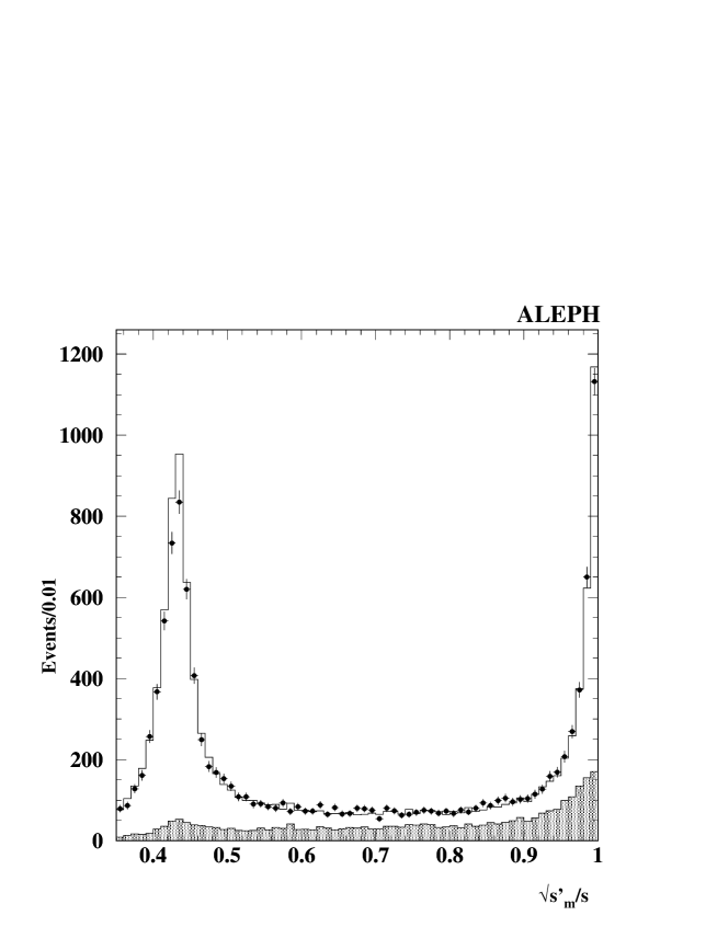
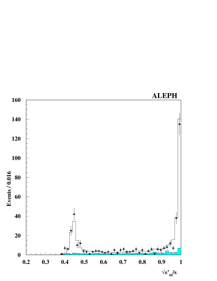
For the exclusive cross sections the events are divided into two hemispheres (hereafter called jets) with respect to the thrust axis, determined after removing the ISR photons. The quantity $\sqrt{s^{\prime}_{m}/s}$ is measured from the reconstructed jet directions and a cut $\sqrt{s^{\prime}_{m}/s}>0.85$ is applied. The $\sqrt{s^{\prime}_{m}/s}$ distribution for the data collected at $\sqrt{s}$=207 GeV is displayed in Fig. 1, together with the expected background. In the exclusive region, the latter is dominated by:

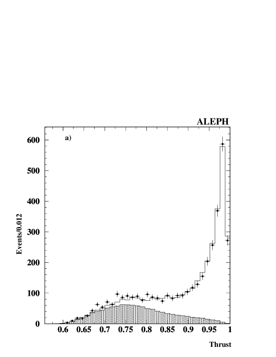
  • W-pair production. For these events, the thrust ($T$) distribution extends to lower values than for ${\mathrm{q}}\bar{\mathrm{q}}$ events, as shown in Fig. 2a. A cut $T>0.85$ rejects approximately $80$% of this background.

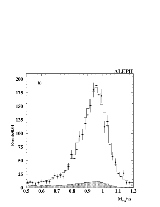
  • Fermion-pair events where, due to photon radiation by both colliding electrons, the measured $\sqrt{s^{\prime}_{m}/s}$ from the jets directions is above 0.85. This background is reduced by requiring that the event visible mass, calculated excluding ISR photons with energies above 10 GeV, is greater than $70$% of the centre-of-mass energy. The residual background is called “radiative background”. Figure 2b shows the visible mass distribution for events with $\sqrt{s^{\prime}/s}\;>\;0.85$ and thrust value exceeding 0.85. The systematic uncertainty on this radiative background accounts for the small discrepancy visible in Fig. 1.

The contribution from four-fermion processes other than WW production is found to be small. It is taken into account by including an additional $0.1$% systematic uncertainty on the exclusive cross section measurements. Other systematic uncertainties arise from the knowledge of the calorimeter calibration and of the detector response to the hadronization process. These uncertainties are taken as fully correlated between years. The evaluation of the detector response uncertainties includes the calorimeter effects described in Ref. [15], which were shown to have negligible impact on this measurement.

The efficiencies for the exclusive process and the background contributions are summarized in Table 2 and the measured cross sections are presented in Table 3.

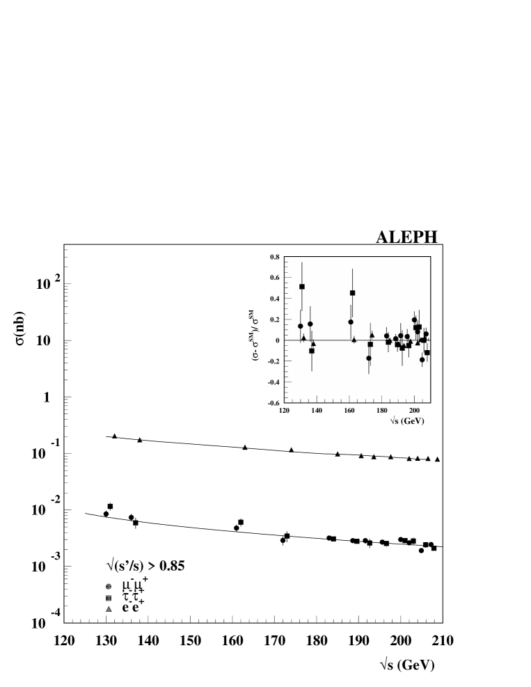
The systematic uncertainties for the inclusive and exclusive processes are listed in Table 4. Figures 3 and 4 show the measured inclusive and exclusive ${\mathrm{q}}\bar{\mathrm{q}}$ cross sections as a function of energy. The exclusive differential cross sections as a function of the thrust axis polar angle are shown in Fig. 5 (in this case the selection efficiencies have been determined in angular bins).

6 Leptonic final states

For the ${\rm e}^{+}{\rm e}^{-}\rightarrow\mu^{+}\mu^{-}$ and ${\rm e}^{+}{\rm e}^{-}\rightarrow\tau^{+}\tau^{-}$ channels, cross section measurements are provided for the inclusive and exclusive processes as defined in Section 4. The inclusive cross sections are determined after background subtraction and a global efficiency correction, while the exclusive cross sections are computed as the sum of the measured cross sections in bins of $\cos\theta$. Asymmetries are extracted by a counting method from the $\cos\theta^{*}$ distributions, where $\theta^{*}$ is the scattering angle between the incoming e- and the outgoing $\ell^{-}$ in the $\ell^{+}\ell^{-}$ rest frame. The asymmetry $A_{\rm FB}$ is defined as:

$$A_{\rm FB}=\frac{N_{\rm F}-N_{\rm B}}{N_{\rm F}+N_{\rm B}}$$

where $N_{\rm F}$ and $N_{\rm B}$ are the numbers of events with the negative lepton in the forward and backward regions, respectively. Acceptance corrections, as well as corrections for asymmetric distributions of the main backgrounds, are determined with Monte Carlo samples.

For the ${\rm e}^{+}{\rm e}^{-}\rightarrow{\rm e}^{+}{\rm e}^{-}$ channel, because of the dominant contribution from the $t$-channel photon exchange, the cross section is provided only for $\sqrt{s^{\prime}/s}>0.85$ over two angular ranges: $-0.9<\cos\theta^{*}<0.9$ and $-0.9<\cos\theta^{*}<0.7$.

For all leptonic channels, the background contamination, estimated from simulation, stems from $\gamma\gamma$ processes, four-fermion final states ${\rm W^{+}W^{-}}$, ${\rm ZZ}$, ${\rm Ze^{+}e^{-}}$ and production of other di-fermion species. As for the hadronic final state, for the exclusive selection only, events reconstructed with $\sqrt{s_{m}^{\prime}/s}>0.85$ but with a $\ell^{+}\ell^{-}$ invariant mass below $0.85\sqrt{s}$ are called radiative event background.

6.1 The $\mu^{+}\mu^{-}$ channel

The selection of muon pairs is described in Ref. [1]. For the inclusive selection, the main background comes from $\gamma\gamma\rightarrow\mu^{+}\mu^{-}$ and is largely reduced by requiring that the invariant mass of the muon pair exceeds $60\ {\rm GeV}/c^{2}$. For the exclusive selection the background from radiative events is removed by asking that the invariant mass of the muon pair exceeds $0.8\sqrt{s}$. The $\sqrt{s^{\prime}_{m}/s}$ distribution for the data collected at $\sqrt{s}$=207 GeV is displayed in Fig. 6.

The $\mu^{+}\mu^{-}$ selection efficiencies, evaluated using the KK Monte Carlo, are listed in Table 5. The main systematic uncertainty is due to the simulation of the muon identification efficiency and is estimated from the difference between data and simulation for the muon identification efficiency in muon-pair events recorded at the Z peak.

The background contamination is also given in Table 5. For the inclusive selection, a major contribution to the systematic uncertainty on the estimated background comes from the normalization of the $\gamma\gamma\rightarrow\mu^{+}\mu^{-}$ process, and is determined by comparing data and Monte Carlo in the $\mu^{+}\mu^{-}$ mass range $15\ {\rm GeV}/c^{2}<M_{\mu^{+}\mu^{-}}<50\ {\rm GeV}/c^{2}$. Other systematic uncertainties on the inclusive background arise from the knowledge of the $\tau^{+}\tau^{-}$, ${\rm W^{+}W^{-}}$, ZZ and ${\rm Ze^{+}e^{-}}$ cross sections, and are at the level of $3$%, $1$%, $5$% and $10$%, respectively. For the exclusive selection, the dominant background systematic uncertainty comes from radiative events, and is estimated from the difference between the data and the Monte Carlo prediction in the region $60<M_{\mu^{+}\mu^{-}}<150$ GeV/$c^{2}$.

The measured cross sections are presented in Table 6 and in Figs. 7 and 8, and compared to the SM prediction from ZFITTER. The dominant contributions to the systematic uncertainties on the cross sections (Table 7) come from the limited statistics of the Monte Carlo samples and from the knowledge of the integrated luminosity, of the muon identification efficiency and of the background contamination.

The differential cross sections are shown in Table 8 and Fig. 9, while the asymmetry results are presented in Table 9 and in Fig. 10. The dominant systematic uncertainty on the asymmetry comes from the statistical error on the Monte Carlo based corrections to the $\mu^{+}\mu^{-}$ acceptance.

6.2 The $\tau^{+}\tau^{-}$ channel

As described in Ref. [1], the selection of tau pairs requires two collimated jets with low charged-track multiplicity. Each event is divided into two hemispheres and is accepted if at least one hemisphere contains a tau candidate decaying into either a muon, or charged hadrons, or charged hadrons plus one or more $\pi^{0}$.

The dominant backgrounds are reduced in the following way. Criteria against the Bhabha process are applied to events containing two high-momentum charged tracks. An additional cut on the polar angle of both tau-jet candidates is introduced ($|\cos\theta|<0.92$), in order to accept only tracks for which the ionisation estimator $dE/dx$, used to reject electron candidates, is accurately determined. WW events are rejected by requiring the acoplanarity angle between the two tau candidates to be smaller than 250 mrad. Di-muon events are removed by demanding that one of the two hemispheres does not contain a muon. Finally, the tau-pair visible invariant mass is required to exceed $25\,{\rm GeV}/c^{2}$ in order to reduce the $\gamma\gamma\to\ell^{+}\ell^{-}$ contamination. The $\sqrt{s^{\prime}_{m}/s}$ distribution for the data collected at $\sqrt{s}$=207 GeV is displayed in Fig. 11.

The resulting selection efficiencies and the total background contamination are listed in Table 10. For the inclusive selection, the systematic uncertainty on the dominant $\gamma\gamma\to\ell^{+}\ell^{-}$ background is estimated by comparing data and Monte Carlo in the $\tau^{+}\tau^{-}$ mass range $15\ {\rm GeV}/c^{2}<M_{\tau^{+}\tau^{-}}<50\ {\rm GeV}/c^{2}$. Bhabha and WW cross section uncertainties amount to $3$% and $1$% respectively. The systematic uncertainty for the exclusive selection is dominated by the limited knowledge of the radiative background cross section. The uncertainty on the latter is determined as the relative difference between the simulated and the observed numbers of $\tau^{+}\tau^{-}$ events selected with a value of $\sqrt{s^{\prime}_{m}/s}$ between 0.5 and 0.8, assumed to be identical for values in excess of 0.85.

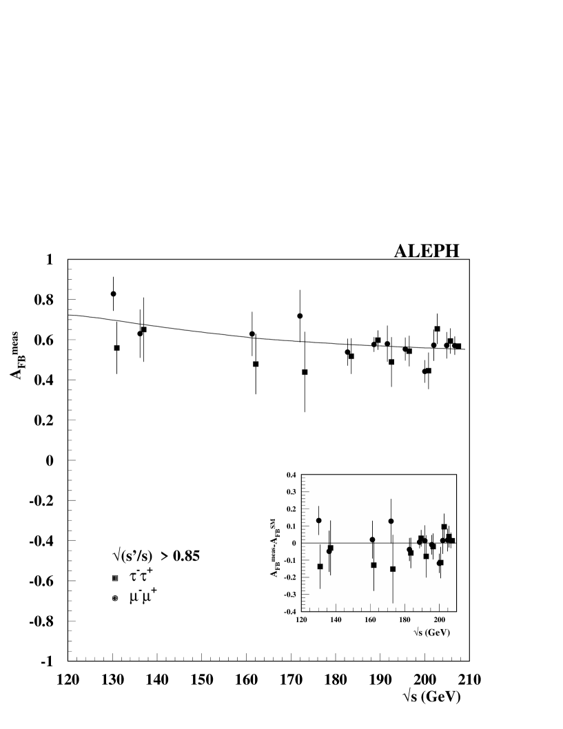
The measured cross sections are presented in Table 11 and Figs. 7 and 8, together with the SM prediction. The systematic uncertainties on these measurements are listed in Table 12. Table 13 and Fig. 12 show the differential cross sections, while the asymmetry results are given in Table 14 and in Fig. 10. Asymmetric contributions from the main backgrounds (Bhabha and radiative events) are significant, and the statistical error on the estimated Bhabha asymmetry yields the dominant systematic uncertainty on the $\tau^{+}\tau^{-}$ asymmetry.

6.3 The ${\rm e}^{+}{\rm e}^{-}$ channel

The selection of electron pairs [1] requires that the two most energetic tracks with opposite sign in the event satisfy the following conditions:
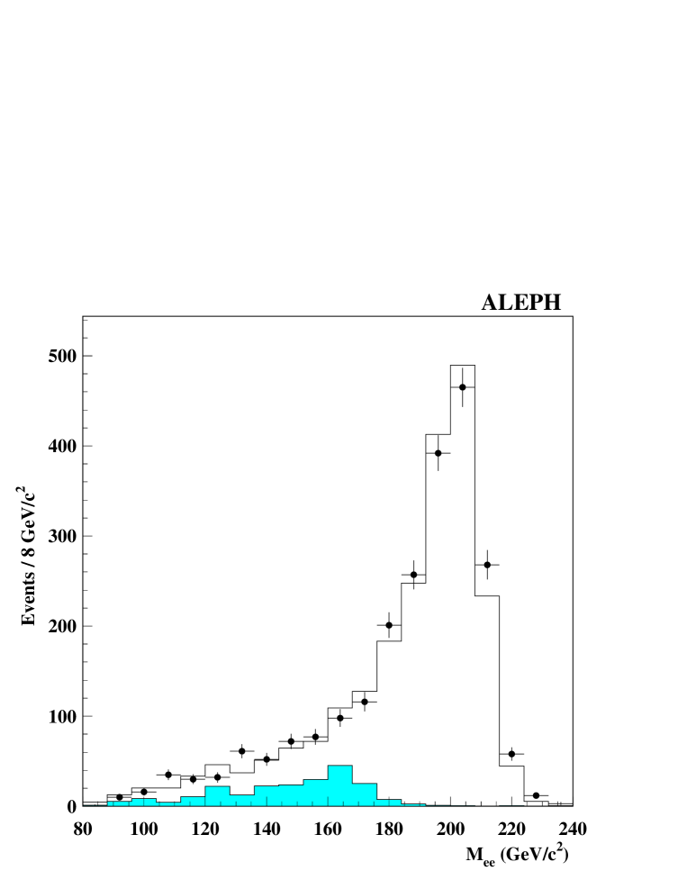
$$\sum_{i=1}^{2}p_{i}>0.30\sqrt{s}\ \ \ \ \ {\rm and}\ \ \ \ \sum_{i=1}^{2}E_{i}>0.40\sqrt{s}\ \ \ \ {\rm and}\ \ \ \ \sum_{i=1}^{2}p_{i}+\mathcal{E}_{i}>1.0\sqrt{s}$$

where $p_{i}$, $E_{i}$ and $\mathcal{E}_{i}$ are the track momentum, the ECAL energy deposition associated to the track, and the total calorimeter energy associated to the track (including the ECAL and HCAL energies as well as the energy from a radiated photon), respectively. The previous cuts reduce significantly the contamination from tau and muon pairs. In addition, events with both tracks identified as muons are discarded. Finally, the requirement on the invariant mass of the ${\rm e}^{+}{\rm e}^{-}$ pair candidate $(M_{{\rm e}^{+}{\rm e}^{-}}>80\ {\rm GeV}/c^{2})$ suppresses most of the residual radiative background. The $M_{{\rm e}^{+}{\rm e}^{-}}$ distribution for the data collected at $\sqrt{s}$=207 GeV is displayed in Fig. 13.

The resulting selection efficiencies and the total background contamination are listed in Table 15. The background is dominated by radiative events whose normalization is extracted from fits to the $M_{{\rm e}^{+}{\rm e}^{-}}$ and $(\Sigma p+\Sigma\mathcal{E})$ experimental distributions using the expected shapes for the ${\rm e}^{+}{\rm e}^{-}$ signal and radiative background. For both selections, $-0.9<\cos\theta^{*}<0.9$ and $-0.9<\cos\theta^{*}<0.7$, the statistical uncertainty on the fit result contributes the dominant systematic uncertainty on the background estimation.

The cross section measurements are compared to the SM prediction from the BHWIDE generator in Table 16 and Fig. 8. The main contributions to the systematic uncertainties are listed in Table 17. Finally, Table 18 and Fig. 14 show the measured differential cross section.

7 Heavy-flavour production

Measurements with heavy-flavour final states are described in this section. The ratios of the $\mathrm{b}\bar{\mathrm{b}}$ and ${\mathrm{c}}\bar{\mathrm{c}}$ cross sections to the hadronic cross section, indicated as $R_{\rm b}$ and $R_{\rm c}$ respectively, are discussed in Sections 7.1 and 7.2. The charge forward-backward asymmetry is measured on a b-enriched ($A_{\rm FB}^{\rm b}$) and a b-depleted ($\langle Q_{\mathrm{FB}}\rangle$) event sample, as presented in Section 7.3.

Results are given for the signal definition as in Ref. [1], with $\sqrt{s^{\prime}/s}\,>\,0.9$ and an angular range restricted to ${\mathrm{|\cos\theta|<\ 0.95}}$. An additional acceptance cut requiring that both jets have ${\mathrm{|}\cos\theta_{\rm jet}|<0.9}$ is applied to ensure that they are contained in the vertex detector acceptance. Table 19 gives the number of selected hadronic events at each centre-of-mass energy. The resulting efficiency is typically 78%, with a dependence on the quark flavour of less than ${\mathrm{\pm 1\%}}$. The background from ${\mathrm{q}}\bar{\mathrm{q}}$ events produced outside the acceptance, but reconstructed inside, is of the order of 2.6% and varies within 0.5% depending on the quark flavour. This variation is taken as systematic uncertainty on the contribution of the radiative background. The total uncertainty of the hadronic selection efficiency in the considered angular range is of the order of 1%.

The long lifetime and large decay multiplicity of b hadrons allow the separation of $\mathrm{b}\bar{\mathrm{b}}$ final states from other quarks. The same tagging variables, complemented by additional variables, can be used to separate ${\mathrm{c}}\bar{\mathrm{c}}$ final states from light quarks. These selections have a moderate dependence on b-quark and c-quark physics modeling uncertainties [17, 18, 19], listed in Tables 20 and 21.
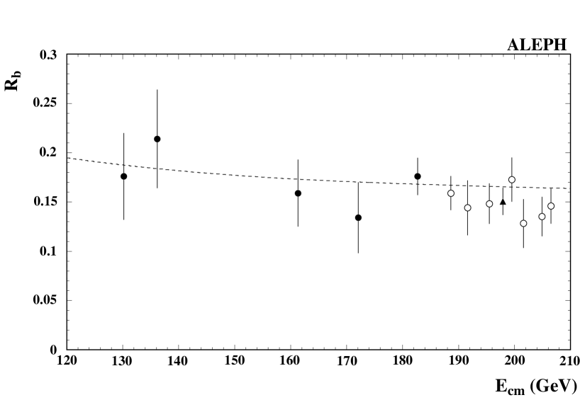
7.1 Measurement of $R_{\rm b}$

Events containing b hadrons are tagged using the procedure developed by ALEPH at LEP1 [20]. For each charged track, a probability (${{\cal{P}}_{T}}$) that it originates at the primary vertex is evaluated using the measured impact parameter significance. This is defined as the signed distance of closest approach of the track to the interaction point divided by the uncertainty on that distance. By taking all tracks or by grouping them according to which hemisphere or which jet they populate, the probability that the event (${{\cal{P}}_{E}}$), the hemisphere (${{\cal{P}}_{H}}$) or the jet (${{\cal{P}}_{J}}$) contains only light-quark jets can be determined. A low value of the probability indicates the presence of long-lived states, which arise dominantly from b-quark production. The b tagging therefore corresponds to a cut on the appropriate probability.

In order to reproduce the detector resolution in the simulation, the procedure to smear the impact parameter significance used for the LEP1 analyses [21] is employed. This is based on the ${\mathrm{\sim\ 3~{}pb^{-1}}}$ calibration data taken at the Z peak each year, in order to optimize the smearing parameters for that year’s data (Fig. 15).

The crucial factor in the determination of $R_{\rm b}$ is the b-tag efficiency. The highly accurate measurements of $R_{\rm b}$ at LEP1 were made possible by the use of a double-tag method, relying on the fact that b-quarks are produced in pairs which populate opposite hemispheres [21]. The use of single- and double-hemisphere tags enables the efficiency, as well as the rate of ${\mathrm{b\bar{b}}}$ production, to be determined from the data, leaving only the level of background to be obtained from the simulation. Furthermore, uncertainties arising from the background knowledge can be minimized with hard cuts.

Unlike at LEP1, the double-tag method is not practical at LEP2 because of the much smaller statistics. For this reason, previous ALEPH measurements of $R_{\rm b}$ at 130-183 GeV [1] were made with a single overall event tag. The efficiency was then determined either directly from the simulation, or by correcting the simulated efficiency by the ratio of the $R_{\rm b}$ value measured with each year Z peak data to the world average. Neither method was satisfactory as they both require an extrapolation (either from the basic simulation or from the Z to LEP2 energies), with mostly unknown related systematic uncertainties.

The full LEP2 data sample, however, has become sufficiently large for an average $R_{\rm b}$ value to be measured with the double-tag procedure, with reduced and controlled systematic uncertainty. An overall efficiency correction can therefore be obtained by taking the ratio of the average values of $R_{\rm b}$ over all centre-of-mass energies, measured with the double- and single-tag methods respectively, so that

$$R^{k}=R^{k}_{s}\frac{\overline{R_{d}}}{\overline{R_{s}}}$$

where $R^{k}$ is the final value of $R_{\rm b}$ at energy $k$, $R^{k}_{s}$ is the value of $R_{\rm b}$ determined by the single-tag procedure at energy $k$, and ${\overline{R_{d}}}$ and ${\overline{R_{s}}}$ are the values of $R_{\rm b}$, averaged over all energy points, as measured with the double- or single-tag method respectively. The above correction, which amounts to about 1.05, assumes that the ratio between the double- and single-tag efficiencies is energy independent, which is true as long as the cuts are not changed on an energy-by-energy basis. It does not require the b-tag cut to be the same for both methods. The optimal selection cut for both the event and hemisphere tags is taken to be the point where the total fractional error on $R_{\rm b}$ is minimized. The b-tag cut corresponds to a b-selection efficiency of 49% (69%) and to a purity of 80% (72%) for the event (hemisphere) tag. The correlation between the single- and double-tag methods is estimated to be 0.95 from the simulation.

The final statistical uncertainty is dominated by the statistical precision on ${\overline{R_{d}}}$. To determine the systematic uncertainty, it is assumed that both the uncertainty for each method and the correlation between them are energy independent. It can then be shown that the relative systematic uncertainty at each energy is given to a good approximation by the relative systematic uncertainty on the average double-tag determination. The systematic uncertainties for the double-tag method are calculated over the full data set, and the contributions are given in Table 22. The dominant sources come from the b-tagging parameters (used to define the track selection and the jet reconstruction) and from the smearing procedure [22]. In addition, by comparing the average efficiency obtained with the double-tag method between data and simulation, the uncertainty on the uds and c backgrounds is found to be smaller than 11%.

The measured average value of $R_{\rm b}$ is

$$R_{\rm b}=0.151\pm 0.012({\rm stat})\pm 0.007({\rm syst})\ \ \ \ (\langle\sqrt{s}\rangle=198\,{\rm GeV})$$

The individual values determined at each energy point are presented in Table 23 and in Fig. 16.

7.2 Measurement of $R_{\rm c}$

The ratio of the ${\mathrm{c}}\bar{\mathrm{c}}$ cross section to the hadronic cross section, $R_{\rm c}$, is measured from the hadronic sample pre-selected as described above.

In a first step, the background from $\mathrm{b}\bar{\mathrm{b}}$ events is reduced to 4% of the hadronic sample with a cut on ${{\cal{P}}_{E}}$ ($\log{\cal P}_{E}>-2$), which retains 86% of the ${\mathrm{c}}\bar{\mathrm{c}}$ events and close to 100% of the light-quark events. The efficiency of this cut is controlled on a sample of WW events, and the resulting systematic uncertainty is about 1%.

The final selection of ${\mathrm{c}}\bar{\mathrm{c}}$ events uses a Neural Network (NN) algorithm trained to separate jets originating from c quarks from jets originating from light quarks. The nine input variables, exploiting the lifetime of D mesons, their masses and their decays into leptons or kaons, are:

  • ${{\cal{P}}_{J}}$, as defined in Section 7.1.

  • The probability that tracks having a high rapidity with respect to the jet axis originate from the primary vertex.

  • The decay length significance of a reconstructed secondary vertex. [23]

  • The $p_{T}$, with respect to the jet axis, of the last track used to build a 2 GeV/$c^{2}$ mass system, tracks being ordered by increasing ${{\cal{P}}_{T}}$.

  • The sum of the rapidities, with respect to the jet axis, of all energy-flow objects within 40 degrees of this axis.

  • The total energy of the four most energetic energy-flow objects in the jet.

  • The missing energy per jet defined as the difference between the beam energy and the reconstructed jet energy.

  • The largest rapidity of lepton candidates with respect to the jet axis.

  • The largest momentum of kaon candidates. Here a charged particle track is identified as a kaon candidate if its ionization energy loss ($dE/dx$) is compatible with that expected from a kaon within three standard deviations, and more compatible with that expected from a kaon than with that expected from a pion.

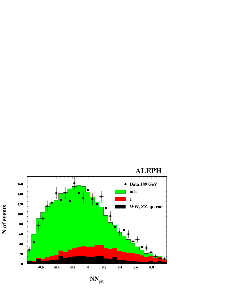
The distribution of the NN output for light-quark jets in the simulation is corrected with the data by comparing enriched samples of light-quark jets selected with a cut applied to the opposite hemisphere. The correction is applied energy by energy. The statistical error on this correction is taken as systematic uncertainty; an additional uncertainty originates from the residual ${\mathrm{c}}\bar{\mathrm{c}}$ background in the selected sample. An example of the distributions used to derive the correction and the correction itself are shown in Fig. 17. A $\mathrm{b}\bar{\mathrm{b}}$-enriched sample is used to control the fraction of $\mathrm{b}\bar{\mathrm{b}}$ background in the final event sample to 5%. Other sources of systematic uncertainties come from the limited statistics of the Monte Carlo samples, the knowledge of the luminosity, detector effects (smearing and momentum corrections), the hadronic pre-selection, and the modeling of c-quark physics. They are listed in Table 24.

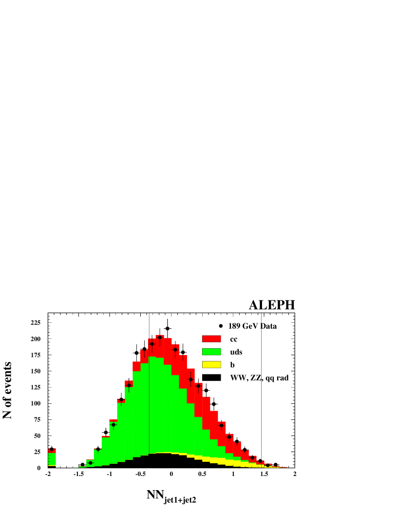
The distribution of the sum of the NN outputs for both jets in the event is shown in Fig. 18. At each energy point, the NN cuts (indicated in Fig. 18 for the $\sqrt{s}$= 189 GeV case) are chosen so as to minimize the total uncertainty. The upper cut suppresses about 5% of the remaining b background with a signal loss of less than 1%. The typical efficiency is 75% with a signal-to-background ratio of 50%. The resulting $R_{\rm c}$ measurements are listed in Table 25.

7.3 Measurements of $A_{\rm FB}^{\rm b}$ and $\langle Q_{\mathrm{FB}}\rangle$

The $A_{\rm FB}^{\rm b}$ and $\langle Q_{\mathrm{FB}}\rangle$ measurements are both extracted from hadronic events pre-selected as described above. A b-enriched sample and a b-depleted sample are obtained using appropriate cuts on ${{\cal{P}}_{E}}$ ($\log{\cal P}_{E}<-4.3$ and $\log{\cal P}_{E}>-2$, respectively). The cuts are set with the aid of the simulation, and correspond to a b content of the order of 90% and 4% for the two samples, respectively. The selection efficiencies vary only slightly with the centre-of-mass energy.

The jet charge ${Q_{\rm jet}}$ of each jet is defined as

$$Q_{\rm jet}=\frac{\sum_{i}q_{i}\cdot p^{\kappa}_{\|,i}}{\sum_{i}p^{\kappa}_{\|,i}}$$

where the sums extend over the reconstructed charged tracks in the jet and $q_{i}$ and $p_{\|,i}$ are the track charge and track momentum parallel to the jet axis, respectively. The parameter ${\mathrm{\kappa}}$ is optimized with simulated events so as to maximize the charge separation between b jets and ${\mathrm{\bar{b}}}$ jets. It is found to be fairly independent of the centre-of-mass energy and the average value of 0.36 is used. The same ${\mathrm{\kappa}}$ value is also used for the b-depleted event sample.

The mean charge asymmetry ${\langle Q_{\rm FB}\rangle\ =\langle Q^{\rm F}_{\rm jet}-Q^{\rm B}_{\rm jet}\rangle}$ is measured on both the b-enriched and b-depleted samples as the average of the jet charge difference between the forward and backward hemispheres, defined with respect to the thrust axis. It is related to the quark forward-backward asymmetries ($A_{\rm FB}^{\rm q}$) as follows

$${{\langle Q_{\rm FB}\rangle\ =\ \frac{\sum\epsilon_{\rm q}\sigma_{\rm q}\delta_{\rm q}A_{\rm FB}^{\rm q}+\sum\epsilon_{\rm x}\sigma_{\rm x}\langle Q_{\rm FB}^{\rm x}\rangle}{\sum\epsilon_{\rm q}\sigma_{\rm q}+\sum\epsilon_{\rm x}\sigma_{\rm x}}}}$$

where the index q indicates the quark flavours (u, d, s, c and b) and the index ${\rm x}$ indicates the various background components (WW, ZZ and radiative ${\mathrm{q\bar{q}}}$). In this expression ${\langle Q_{\rm FB}^{\rm x}\rangle}$ indicates the background mean charge asymmetry , ${\epsilon_{\rm q,x}}$ the selection efficiencies and ${\delta_{\rm q}}$ the charge separation (defined as the mean of the ${Q_{\rm q}-Q_{\rm{\bar{q}}}}$ distribution).

The asymmetry $A_{\rm FB}^{\rm b}$ is obtained from the b-enriched sample; it is extracted from ${\langle Q_{\rm FB}^{\rm enr}\rangle}$, the charge asymmetry measured from the data, using the previous formula. The background mean charge asymmetry, the selection efficiencies and the charge separations are taken from the simulation. The non-b quark cross sections ${\mathrm{\sigma_{q}}}$ and asymmetries $A_{\rm FB}^{\rm q}$ are computed with ZFITTER for the signal definition $\sqrt{s^{\prime}/s}$ ${\mathrm{>}}$ 0.9, with ${\mathrm{|\cos\theta|<0.9}}$ for both quark and anti-quark. It is possible to reduce the dependence of this measurement on the b efficiency estimated from the simulation by replacing the product ${\mathrm{\epsilon_{b}\sigma_{b}}}$ with ${N_{\rm data}^{\rm b}/{\cal L}}$, where ${N_{\rm data}^{\rm b}}$ is the number of b events in the data and ${\mathrm{{\cal L}}}$ is the integrated luminosity. It follows:

$${{A_{\rm FB}^{\rm b}\ =\ \frac{N_{\rm data}^{\rm b}\langle Q_{\rm FB}^{\rm enr}\rangle-\sum^{\rm q\neq b}{\cal L}\epsilon_{\rm q}\sigma_{\rm q}\delta_{\rm q}A_{\rm FB}^{\rm q}-\sum{\cal L}\epsilon_{\rm x}\sigma_{\rm x}\langle Q_{\rm FB}^{\rm x}\rangle}{(N_{\rm data}^{\rm b}-N_{\rm MC}^{\rm bkg})\delta_{\rm b}}}}$$

where ${N_{\rm MC}^{\rm bkg}}$ is the number of background events predicted by the simulation. The measurement is corrected by a factor 1.03 to extrapolate from the range ${\mathrm{|\cos\theta|<0.9}}$ to the nominal range ${\mathrm{|\cos\theta|<0.95}}$. The potentially large uncertainty originating from the ${\mathrm{c}}\bar{\mathrm{c}}$ contamination in the b-enriched sample is reduced to a negligible level by a tight cut on ${{\cal{P}}_{E}}$.

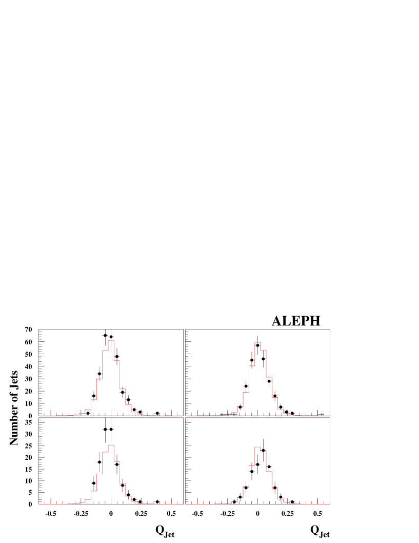
In order to evaluate the systematic uncertainty on the jet charge separation, $\delta_{q}$ is measured with the data, using semileptonic b decays for b quarks and semileptonic WW events for light and c quarks. Semileptonic b decays are selected by requiring an electron or muon with high transverse momentum in one jet. The charge of the opposite b jet is then known. Because of the low event statistics surviving this selection, data taken at all energies must be combined. The difference between the jet charge distributions in data and simulation (Fig. 19) is propagated as systematic uncertainty to the $A_{\rm FB}^{\rm b}$ measurement, representing the dominant systematic effect. A similar procedure is applied to a selected sample of semileptonic W-pair events to measure the average lighter quarks charge separation.

These and other sources of systematic uncertainties are summarized in Table 26. The $A_{\rm FB}^{\rm b}$ measurements are presented in Table 27.

Finally, the difference ${\Delta\ =\ \langle Q_{\rm FB}^{\rm depl}\rangle-\langle Q_{\rm FB}^{\rm MC}\rangle}$, measured with b-depleted samples, constrains simultaneously $A_{\rm FB}^{\rm q}$ and ${\mathrm{\sigma_{q}}}$ (q=u,d,s or c), providing additional sensitivity to physics beyond the Standard Model. Assuming small deviations from the SM, the linearized equation

$${\mathrm{\Delta}=\sum_{\rm q}\frac{\partial\langle Q_{\rm FB}\rangle}{\partial\sigma_{\rm q}}\Delta\sigma_{\rm q}+\sum_{\rm q}\frac{\partial\langle Q_{\rm FB}\rangle}{\partial A^{\rm q}_{\rm FB}}\Delta A^{\rm q}_{\rm FB}}$$

is used to constrain the deviations of $A_{\rm FB}^{\rm q}$ and ${\mathrm{\sigma_{q}}}$ from the SM with the measured values of $\Delta$ at each centre-of-mass energy, as described in Ref. [1]. Examples of the coefficients of the above equations are shown in Table 28.

The dominant systematic uncertainty originates from the jet charge, determined as explained above. This and other sources are listed in Table 29, while the measurement results are reported in Table 30.

8 Interpretation in terms of new physics

New physics, if present, could give rise to deviations of the measured cross sections and asymmetries from the Standard Model expectations. The results presented in the previous Sections indicate good agreement between the data and the SM predictions. As an example the global fit of the muon, tau and hadronic exclusive cross sections and of the muon and tau asymmetries at the seven energies gives $\chi^{2}/{\rm d.o.f.}=29.79/35$. Stringent limits can be placed on scenarios beyond the Standard Model.

Predictions of several models of new physics are fitted to the data using binned maximum likelihoods, as explained in [1]. For this purpose, the measurements described in this paper are combined with those at lower energies reported in [1].

Following the conclusions in Ref. [24], theoretical uncertainties of 0.26%, 0.4%, 0.4%, 0.5% and 2.0% are assigned to the ${\mathrm{q}}\bar{\mathrm{q}}$, ${\mathrm{\mu^{+}\mu^{-}}}$, ${\mathrm{\tau^{+}\tau^{-}}}$, ${\mathrm{e}}^{+}{\mathrm{e}}^{-}$ (forward) and ${\mathrm{e}}^{+}{\mathrm{e}}^{-}$ (central) cross section predictions, respectively.

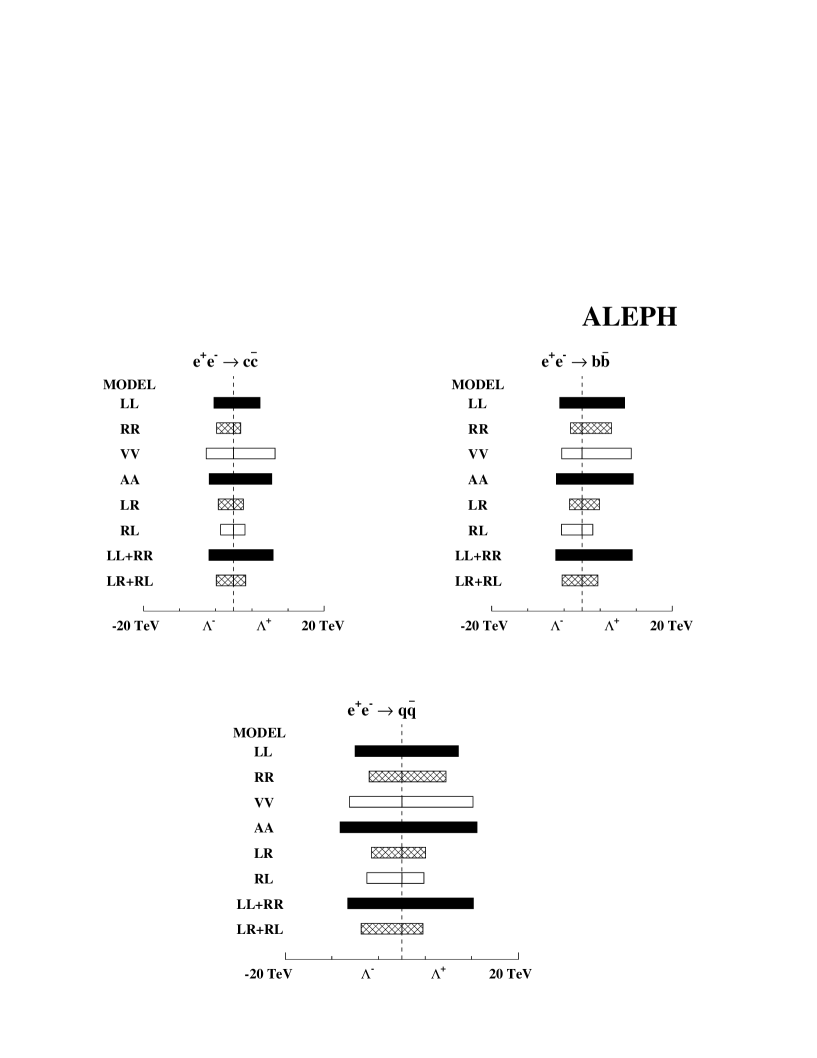
8.1 Contact interactions

Four-fermion contact interactions, expected to occur for example if fermions are composite, are characterized by a scale $\Lambda$, interpreted as the mass of a new heavy particle exchanged between the incoming and outgoing fermions, and a coupling g giving the strength of the interaction. Conventionally, $g$ is assumed to satisfy $g/\sqrt{4\pi}=1$. Following the notation of Ref. [25], the effective Lagrangian for the four-fermion contact interaction in the process ${\mathrm{e^{+}e^{-}\rightarrow f\bar{f}}}$ is given by

$$L^{\rm CI}=\frac{g^{2}\eta_{\rm sign}}{(1+\delta)\Lambda^{2}}\sum_{i,j={\rm L,R}}\eta_{ij}[\bar{e}_{i}\gamma^{\mu}e_{i}][\bar{f}_{j}\gamma_{\mu}f_{j}]$$

with $\delta$ = 1 if $f=e$ and $\delta$ = 0 otherwise. The fields $e_{\rm L,R}\ (f_{\rm L,R})$ are left- or right-handed projections of electron (fermion) spinors, and the coefficients $\eta_{ij}$ specify the relative contribution of the different chirality combinations. New physics can add constructively or destructively to the SM Lagrangian, according to the sign of $\eta_{\rm sign}$. Several models, defined in Table 31, are considered in this analysis.

In the presence of contact interactions, the differential cross section for ${\mathrm{e^{+}e^{-}\rightarrow f\bar{f}}}$ as a function of the polar angle $\theta$ of the outgoing fermion with respect to the e- beam can be written as

$$\frac{{\mathrm{d}}\sigma}{{\mathrm{d}}\cos\theta}=F_{\mathrm{SM}}(s,t)\left[1+\mbox{$\epsilon$}\frac{F_{\mathrm{IF}}^{\mathrm{Born}}(s,t)}{F_{\mathrm{SM}}^{\mathrm{Born}}(s,t)}+\mbox{$\epsilon$}^{2}\frac{F_{\mathrm{CI}}^{\mathrm{Born}}(s,t)}{F_{\mathrm{SM}}^{\mathrm{Born}}(s,t)}\right]$$

where $s,t$ are the Mandelstam variables and $\mbox{$\epsilon$}=g^{2}\eta_{\mathrm{sign}}/(4\pi\mbox{$\Lambda$}^{2})$. $F_{\mathrm{SM}}$ is the Standard Model cross section. $F_{\mathrm{IF}}^{\mathrm{Born}}$ and $F_{\mathrm{CI}}^{\mathrm{Born}}$ are the contributions from the interference between the Standard Model and the contact interaction and from the pure contact interaction, respectively. The above formula is fitted to the data using a binned maximum likelihood function, as described in Ref. [1]. Limits are quoted at the 95% C.L. for $\Lambda^{\pm}$ corresponding to $\eta_{\rm sign}=\pm 1$.

For leptonic final states, limits on the scale $\Lambda$ are derived from the leptonic differential cross sections. The results are shown in Table 32 and Fig. 20.

For generic hadronic final states, limits on $\Lambda$ are obtained from fits to the hadronic cross sections assuming that the contact interaction affects all flavours with equal strength. In addition, limits on models involving only couplings to c or b quarks can be derived from the $R_{\rm c}$ and $Q_{\rm FB}^{\rm depl}$ or $R_{\rm b}$ and $A_{\rm FB}^{\rm b}$ measurements respectively. The results are shown in Table 33 and Fig. 21. Combining hadronic cross section measurements with observables in the charm sector improves the overall sensitivity, whereas the gain is marginal for the bottom sector.

In summary, the ALEPH limits on the scale of contact interactions $\Lambda$ are in the range 2-17 TeV, and most stringent for the VV and AA models. Constraints on ${\mathrm{e^{+}e^{-}\ell^{+}\ell^{-}}}$, ${\mathrm{e^{+}e^{-}b\bar{b}}}$ and ${\mathrm{e^{+}e^{-}c\bar{c}}}$ contact interactions are of particular interest because these couplings are not accessible at ${\mathrm{p\bar{p}}}$ and ${\mathrm{ep}}$ colliders.

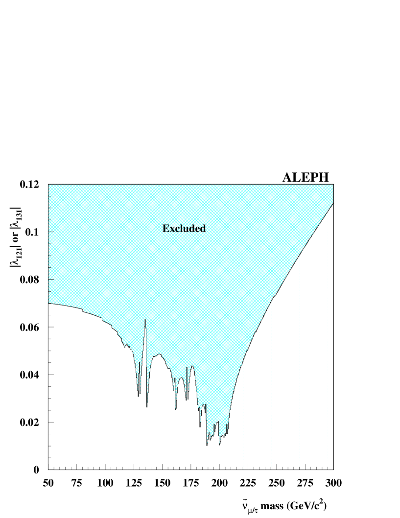
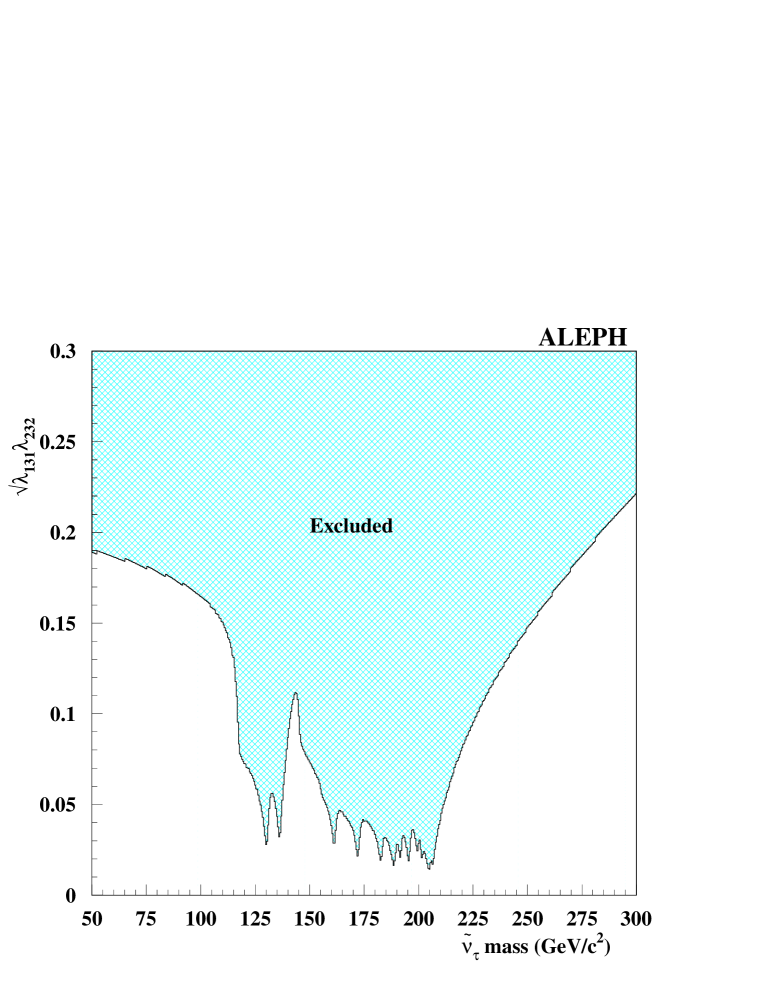
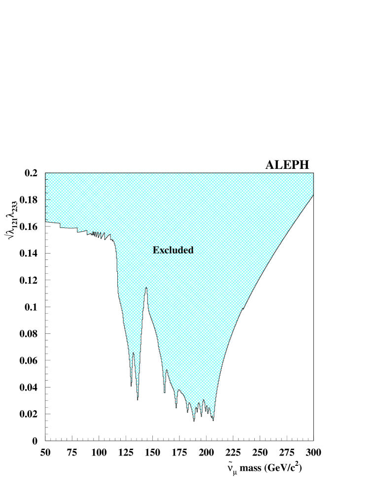
8.2 R-parity violating sneutrinos

Supersymmetric theories with R-parity violation have terms in the Lagrangian of the form ${\lambda_{ijk}{\rm L}_{i}{\rm L}_{j}\bar{\rm E}_{k}}$, where L denotes a left-handed lepton doublet superfield and ${\mathrm{\bar{E}}}$ a right-handed lepton singlet superfield [26]. The parameters ${\mathrm{\lambda}}$ are Yukawa couplings and $i,j,k$ are generation indices. The couplings ${\lambda_{ijk}}$, assumed to be real in this analysis, are non-vanishing only for $i<j$. These terms allow for single production of sleptons in ${\mathrm{e^{+}e^{-}}}$ collisions.

At LEP, R-parity violating sneutrinos could be exchanged in the $s$ or $t$ channel, leading to deviations of di-lepton production from the SM expectations. Table 34 shows the most interesting cases. Sneutrino exchange in the $s$ channel gives rise to a resonant state, assumed here to have a width of 1 GeV/$c^{2}$ [26]. Limits on couplings are extracted as explained in Ref. [1] using leptonic differential cross section measurements. Figures 22-24 show the resulting constraints for processes involving sneutrino exchange.

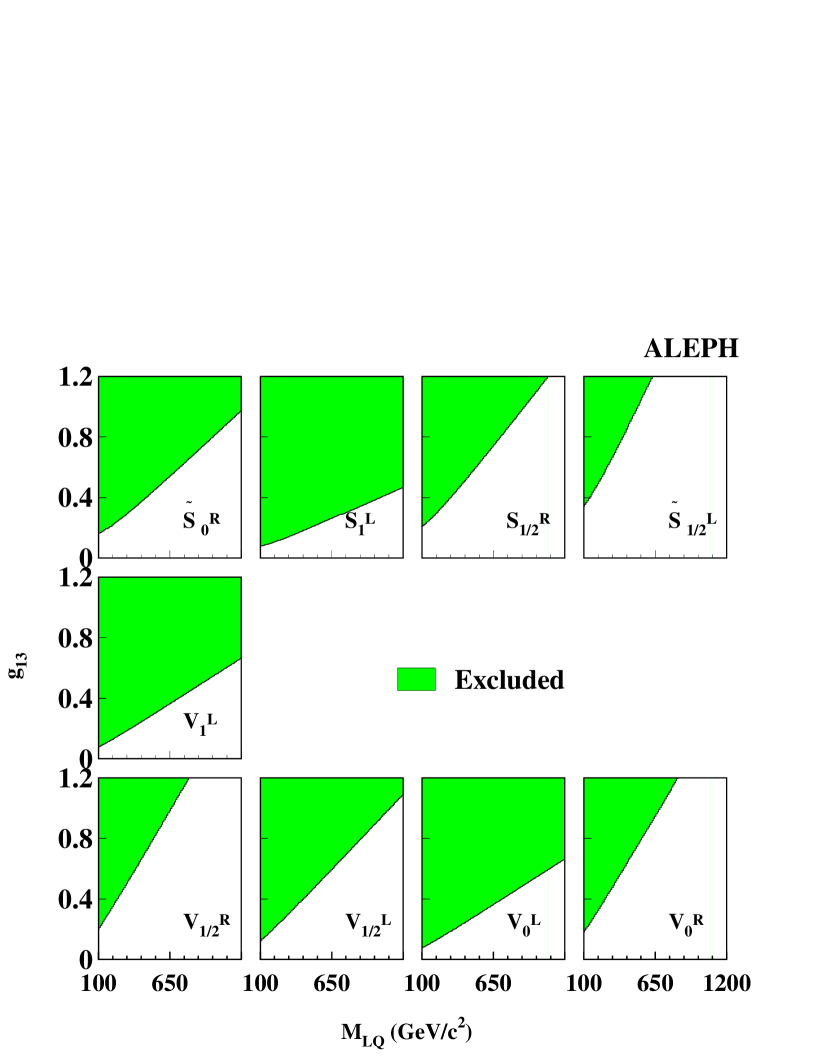
8.3 Leptoquarks and R-Parity violating squarks

At LEP, the $t$ channel exchange of a leptoquark can modify the ${\mathrm{q}}\bar{\mathrm{q}}$ cross section and jet charge asymmetry. In scenarios where leptoquarks couple to the first-generation leptons and to the second- or third-generation quarks, more stringent limits can be placed by using in addition the relevant heavy-flavour observables $R_{\rm b}$, $R_{\rm c}$ and $A_{\rm FB}^{\rm b}$. Comparisons of the measurements with the predictions given in Ref. [27] allow upper limits to be set on the leptoquark coupling as a function of its mass.

Leptoquarks are classified according to the spin, weak isospin I and hypercharge. Scalar and vector leptoquarks are denoted by symbols ${\mathrm{S_{I}}}$ and ${\mathrm{V_{I}}}$, and different hypercharge states are indicated by a tilde. In addition, “L” or “R” specifies if the leptoquark couples to the right- or left-handed leptons exclusively. The ${\mathrm{\tilde{S}_{\frac{1}{2}}(L)}}$ and ${\mathrm{S_{0}(L)}}$ leptoquarks are equivalent to up-type anti-squarks and down-type squarks, respectively, in supersymmetric theories with an R-parity breaking term ${\lambda^{\prime}_{1jk}{\rm L}_{1}{\rm Q}_{j}\bar{\rm D}_{k}}$ ($j,k$=1,2,3). Limits on leptoquark couplings are then equivalent to limits on ${\lambda_{1jk}}$.

Table 35 gives, for various leptoquark type, the 95% C.L. lower limit on the mass $M_{\rm LQ}$ assuming the leptoquark couples with strength $g^{2}=4\pi$ $\alpha_{em}^{2}$. Figure 25 shows the exclusion contour in the plane coupling-mass for leptoquarks coupling to the third quark generation.

8.4 Extra Z bosons

Several extensions to the Standard Model [28] predict the existence of at least one additional neutral gauge boson Z. Two classes of models are considered here: $E_{6}$ models and Left-Right (LR) models. In $E_{6}$ models, the Z properties depend on the breaking pattern of the gauge symmetry, governed by the parameter $\theta_{6}$. Limits on the Z mass are derived here for the choices $\theta_{6}=0,\,\pi/2,\,\pm\arctan\sqrt{5/3}$, known as the $\chi,\,\psi,\,\eta$ and $I$ models. In LR models, right-handed extensions to the Standard Model gauge group are introduced. The Z couplings to fermions depend on the parameter $\alpha_{\rm LR}$, which is set here to the value $\alpha_{\rm LR}=1.53$ (as predicted in LR symmetric models). More details can be found in [1].

Limits on the Z mass are derived using the method described in Ref. [1]. The theoretical predictions for the two-fermion exclusive cross-sections and asymmetries are obtained from ZFITTER 6.10 used together with ZEFIT [29] and they are compared to the corresponding measurements presented above.

The most conservative $m_{\rm Z^{\prime}}$ lower limits, with respect to the Z/Z mixing angle, are presented in Table 36. Constraints on extra gauge boson have been also set at the Tevatron [30, 31, 32].

8.5 Limits on TeV-scale gravity

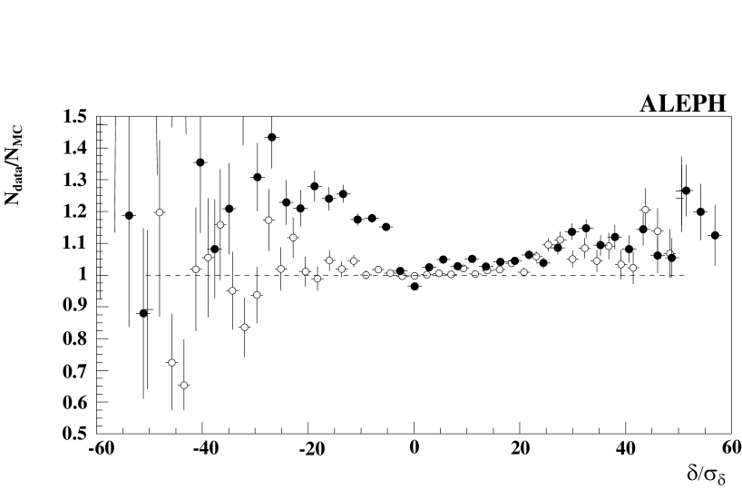
A solution to the hierarchy problem has been proposed in Ref. [33], where gravity is characterized by a fundamental scale $M_{\rm D}$ which could be as low as 1 TeV, provided that space has ${\mathrm{\delta}}$ extra dimensions compactified to a size $R$. The effective Gravitational constant is then given by ${g_{\rm N}^{-1}=8\pi R^{\delta}M_{\rm D}^{2+\delta}}$. Hence, gravity can become strong at small distances, leading for example to deviations of the ${\mathrm{e^{+}e^{-}\rightarrow\ e^{+}e^{-}}}$ differential cross section from the SM expectation. These deviations are parametrized by a cut-off ${\mathrm{\Lambda_{T}}}$ [34] of the same order of magnitude as $M_{\rm D}$.

Figure 26 shows the ${\mathrm{e^{+}e^{-}\ \rightarrow\ e^{+}e^{-}}}$ differential cross sections measured with data collected at $\sqrt{s}$=189-209 GeV, normalized to the SM prediction, together with the expected deviations from TeV-scale gravity models. Using all data, a lower limit of 1.1 TeV (1.2 TeV) is obtained on ${\mathrm{\Lambda_{T}^{-}}}$ (${\mathrm{\Lambda_{T}^{+}}}$), for destructive (constructive) interference with the SM prediction. In computing the limits the luminosity measurement was assumed unaffected and the theoretical errors of 0.5% (2.0%) assigned to the forward (central) ${\mathrm{e^{+}e^{-}}}$ cross sections were taken as uncorrelated.

9 Conclusions

Several measurements of di-fermion final states using data collected by ALEPH at $\sqrt{s}$=189-209 GeV have been presented. In the leptonic sector, total and differential cross sections, as well as muon and tau forward-backward asymmetries, have been derived. In the hadronic sector, cross sections, forward-backward charge asymmetries for light and c quarks, b quark forward-backward asymmetries, and the $R_{\rm b}$ and $R_{\rm c}$ ratios have been measured. Similar measurements have been performed by the DELPHI [35], L3 [36] and OPAL [37] Collaborations.

The results are consistent with the Standard Model expectations and have been used to place constraints on several scenarios of new physics: four-fermion contact interactions, R-parity violating sneutrinos and squarks, leptoquarks, additional Z bosons and TeV-scale gravity. These constraints improve on previous ALEPH limits, and are similar to those obtained by the other LEP Collaborations.

Additional interpretations in terms of new physics, using measurements presented in this paper, can be found in Refs. [38, 39].

Acknowledgments

We thank our colleagues from the CERN accelerator divisions for the successful running of LEP at high energy. We are indebted to the engineers and technicians in all our institutions for their contribution to the good performance of ALEPH. Those of us from non-member states thank CERN for its hospitality.

Table 1: Luminosity weighted centre-of-mass energies and integrated luminosities for the data samples presented in this paper. The total (statistical and systematic combined) uncertainties on the integrated luminosities are given. The last column contains the data sample names used in this paper.
Year $E_{\rm cm}$ (GeV) Luminosity (${\mathrm{pb^{-1}}}$)
1998 188.63 174.2 $\rm\pm$ 0.8 189
1999 191.58 28.9 $\rm\pm$ 0.1 192
195.52 79.9 $\rm\pm$ 0.4 196
199.52 86.3 $\rm\pm$ 0.4 200
201.62 41.9 $\rm\pm$ 0.2 202
2000 204.86 81.60$\rm\pm$ 0.4 205
206.53 133.6 $\rm\pm$ 0.6 207
Table 2: Selection efficiencies and background fractions for the $\rm{q\overline{q}}$ channel for the inclusive and exclusive processes, as a function of the centre-of-mass energy. The statistical uncertainties are also given.
$\sqrt{s^{\prime}/s}$ $E_{\rm cm}$ Efficiency Background
cut (GeV) (%) (%)
0.1 189 $83.9\pm 0.2$ $20.2\pm 0.1$
192 $83.9\pm 0.3$ $22.2\pm 0.1$
196 $83.3\pm 0.3$ $22.2\pm 0.1$
200 $82.5\pm 0.3$ $22.1\pm 0.1$
202 $82.3\pm 0.3$ $22.3\pm 0.1$
205 $81.4\pm 0.3$ $23.3\pm 0.1$
207 $81.1\pm 0.3$ $23.7\pm 0.1$
0.85 189 $81.9\pm 0.3$ $5.82\pm 0.07$
$|\cos\theta|<0.95$ 192 $82.2\pm 0.3$ $6.10\pm 0.08$
196 $82.3\pm 0.3$ $6.34\pm 0.08$
200 $82.5\pm 0.3$ $6.56\pm 0.08$
202 $83.3\pm 0.3$ $6.93\pm 0.08$
205 $82.0\pm 0.3$ $8.47\pm 0.09$
207 $81.9\pm 0.3$ $8.69\pm 0.09$
Table 3: Measured $\rm{q\overline{q}}$ cross sections for the inclusive and exclusive processes, as a function of the centre-of-mass energy, with their statistic and systematic uncertainties. The corresponding Standard Model predictions from ZFITTER are given in the last column.
$\sqrt{s^{\prime}/s}$ ${E_{\rm cm}}$ Number $\sigma_{\rm{q\overline{q}}}$ SM prediction
cut (GeV) of events (pb) (pb)
0.1 189 18617 $101.65\pm 0.83\pm 0.83$ 99.35
192 2898 $93.00\pm 1.95\pm 0.73$ 95.41
196 7776 $90.89\pm 1.17\pm 0.66$ 90.55
200 8102 $88.65\pm 1.12\pm 0.63$ 86.02
202 3710 $83.59\pm 1.56\pm 0.63$ 83.78
205 6989 $80.71\pm 1.12\pm 0.46$ 80.53
207 11183 $79.16\pm 0.85\pm 0.43$ 78.94
0.85 189 3153 $20.80\pm 0.38\pm 0.17$ 20.58
$|\cos\theta|<0.95$ 192 508 $20.07\pm 0.92\pm 0.16$ 19.72
196 1329 $18.93\pm 0.54\pm 0.16$ 18.67
200 1367 $17.94\pm 0.51\pm 0.16$ 17.69
202 658 $17.56\pm 0.71\pm 0.15$ 17.21
205 1238 $16.94\pm 0.52\pm 0.15$ 16.51
207 1958 $16.34\pm 0.38\pm 0.14$ 16.16
Table 4: Contributions to the systematic uncertainties (in %) on the measured $\rm{q\overline{q}}$ cross sections, averaged among the centre-of-mass energies.
Source $\sqrt{s^{\prime}/s}$ cut
0.1 0.85
MC statistics 0.30 0.30
Energy scale 0.36 0.30
Detector response 0.38 0.60
${\gamma\gamma\to\rm{q\overline{q}}}$ 0.05
WW 0.19 0.05
Radiative background 0.21
Other 4-f backgrounds 0.03
Luminosity 0.45 0.45
Total 0.78 0.89
Table 5: Selection efficiencies and background fractions for the ${\mathrm{\mu^{+}\mu^{-}}}$ channel for the inclusive and exclusive processes. The statistical uncertainties are also given.
$\sqrt{s^{\prime}/s}$ ${E_{\rm cm}}$ Efficiency Background
cut ${\mathrm{(GeV)}}$ (${\mathrm{\%}}$) (${\mathrm{\%}}$)
0.1 189 $74.7\pm 0.2$ $8.2\pm 0.5$
192 $75.1\pm 0.2$ $7.6\pm 0.6$
196 $74.6\pm 0.1$ $9.0\pm 0.7$
200 $74.1\pm 0.1$ $10.4\pm 0.8$
202 $74.0\pm 0.2$ $10.0\pm 0.8$
205 $73.5\pm 0.1$ $11.1\pm 0.9$
207 $73.1\pm 0.1$ $11.8\pm 1.0$
0.85 189 $95.8\pm 0.1$ $1.8\pm 0.1$
$|\cos\theta|<0.95$ 192 $96.1\pm 0.1$ $1.9\pm 0.1$
196 $96.1\pm 0.1$ $1.9\pm 0.1$
200 $96.1\pm 0.1$ $1.9\pm 0.1$
202 $96.2\pm 0.1$ $1.9\pm 0.1$
205 $96.1\pm 0.1$ $2.1\pm 0.1$
207 $95.9\pm 0.12$ $1.9\pm 0.1$
Table 6: Measured ${\mathrm{\mu^{+}\mu^{-}}}$ cross sections for the inclusive and exclusive processes. The numbers of selected events and the predicted SM cross sections from ZFITTER are also given.
$\sqrt{s^{\prime}/s}$ ${E_{\rm cm}}$ Number $\sigma_{\rm{\mu^{+}\mu^{-}}}$ ${\mathrm{SM}}$ ${\mathrm{prediction}}$
cut ${\mathrm{(GeV)}}$ of events ${\mathrm{(pb)}}$ ${\mathrm{(pb)}}$
0.1 189 1090 $7.68\pm 0.26\pm 0.06$ $7.78$
192 189 $8.04\pm 0.66\pm 0.07$ $7.50$
196 493 $7.53\pm 0.39\pm 0.07$ $7.15$
200 489 $6.85\pm 0.36\pm 0.07$ $6.83$
202 238 $6.92\pm 0.52\pm 0.07$ $6.66$
205 402 $5.96\pm 0.35\pm 0.06$ $6.43$
207 683 $6.16\pm 0.28\pm 0.07$ $6.31$
0.85 189 489 $2.88\pm 0.13\pm 0.02$ $2.83$
$|\cos\theta|<0.95$ 192 81 $2.86\pm 0.33\pm 0.02$ $2.73$
196 211 $2.70\pm 0.19\pm 0.02$ $2.61$
200 252 $2.99\pm 0.20\pm 0.02$ $2.50$
202 107 $2.64\pm 0.26\pm 0.02$ $2.44$
205 154 $1.92\pm 0.16\pm 0.02$ $2.36$
207 321 $2.46\pm 0.14\pm 0.02$ $2.32$
Table 7: Contributions to the systematic uncertainties (in %) on the measured ${\mathrm{\mu^{+}\mu^{-}}}$ cross sections, averaged among the centre-of-mass energies.
Source $\sqrt{s^{\prime}/s}$ cut
0.1 0.85
MC statistics 0.76 0.17
Muon identification 0.20 0.20
Background contamination 0.20 0.53
Luminosity 0.45 0.45
Total 0.93 0.75
Table 8: Measured differential cross section (pb) for the ${\mathrm{\mu^{+}\mu^{-}}}$ channel for $\sqrt{s^{\prime}/s}>0.85$, as a function of the polar angle of the negative muon with respect to the incoming electron. Statistical and systematic uncertainties are combined.
${E_{\rm cm}}$ (GeV)
$\cos\theta$ 189 192 196 200 202 205 207
$[-0.95,-0.80]$ $0.7\pm 0.1$ $0.2\pm 0.3$ $0.5\pm 0.2$ $0.7\pm 0.2$ $0.8\pm 0.3$ $0.3\pm 0.2$ $0.5\pm 0.2$
$[-0.80,-0.60]$ $0.3\pm 0.1$ $0.2\pm 0.3$ $0.6\pm 0.2$ $0.6\pm 0.3$ $0.1\pm 0.2$ $0.3\pm 0.2$ $0.4\pm 0.1$
$[-0.60,-0.40]$ $0.4\pm 0.1$ $1.1\pm 0.3$ $0.5\pm 0.2$ $0.9\pm 0.2$ $0.9\pm 0.2$ $0.2\pm 0.2$ $0.2\pm 0.1$
$[-0.40,-0.20]$ $0.8\pm 0.2$ $0.7\pm 0.4$ $0.6\pm 0.2$ $1.0\pm 0.2$ $0.5\pm 0.3$ $0.3\pm 0.2$ $1.0\pm 0.2$
$[-0.20,\,\,\,\,\,0.00]$ $1.1\pm 0.2$ $0.9\pm 0.4$ $0.9\pm 0.2$ $1.2\pm 0.2$ $0.7\pm 0.3$ $1.0\pm 0.2$ $0.6\pm 0.2$
$[\,\,\,\,\,0.00,\,\,\,\,\,0.20]$ $1.1\pm 0.2$ $1.8\pm 0.5$ $1.1\pm 0.3$ $1.5\pm 0.3$ $1.2\pm 0.4$ $1.1\pm 0.3$ $1.0\pm 0.2$
$[\,\,\,\,\,0.20,\,\,\,\,\,0.40]$ $2.1\pm 0.2$ $0.9\pm 0.6$ $1.9\pm 0.3$ $1.9\pm 0.3$ $1.7\pm 0.4$ $1.2\pm 0.3$ $1.7\pm 0.2$
$[\,\,\,\,\,0.40,\,\,\,\,\,0.60]$ $2.0\pm 0.3$ $1.9\pm 0.6$ $2.4\pm 0.4$ $1.8\pm 0.3$ $2.4\pm 0.5$ $1.7\pm 0.3$ $1.9\pm 0.3$
$[\,\,\,\,\,0.60,\,\,\,\,\,0.80]$ $3.3\pm 0.3$ $3.8\pm 0.7$ $2.8\pm 0.4$ $3.1\pm 0.4$ $2.1\pm 0.6$ $1.8\pm 0.4$ $2.9\pm 0.3$
$[\,\,\,\,\,0.80,\,\,\,\,\,0.95]$ $3.8\pm 0.4$ $3.8\pm 0.9$ $3.2\pm 0.5$ $3.4\pm 0.5$ $3.8\pm 0.7$ $2.4\pm 0.5$ $2.9\pm 0.4$
Table 9: Measured ${\mathrm{\mu^{+}\mu^{-}}}$ forward-backward asymmetry for $\sqrt{s^{\prime}/s}>0.85$ and in the range $|\cos\theta|<0.95$. The SM prediction from ZFITTER is given in the last column.
${E_{\rm cm}}$ (GeV) $A_{\rm FB}^{\rm{\mu^{+}\mu^{-}}}$ ${\mathrm{SM}}$ ${\mathrm{prediction}}$
189 $0.576\pm 0.036\pm 0.009$ $0.570$
192 $0.580\pm 0.090\pm 0.009$ $0.567$
196 $0.553\pm 0.057\pm 0.006$ $0.563$
200 $0.442\pm 0.056\pm 0.006$ $0.560$
202 $0.573\pm 0.078\pm 0.010$ $0.558$
205 $0.572\pm 0.066\pm 0.010$ $0.555$
207 $0.570\pm 0.046\pm 0.007$ $0.554$
Table 10: Selection efficiencies and background fractions for the ${\mathrm{\tau^{+}\tau^{-}}}$ channel for the inclusive and exclusive processes. The statistical uncertainties are also given.
$\sqrt{s^{\prime}/s}$ ${E_{\rm cm}}$ Efficiency Background
cut ${\mathrm{(GeV)}}$ (${\mathrm{\%}}$) (${\mathrm{\%}}$)
0.1 189 $42.6\pm 0.2$ $12.4\pm 0.5$
192 $42.0\pm 0.2$ $12.9\pm 0.4$
196 $41.7\pm 0.2$ $14.4\pm 0.5$
200 $41.5\pm 0.2$ $13.9\pm 0.5$
202 $41.4\pm 0.2$ $15.9\pm 0.6$
205 $41.2\pm 0.2$ $15.5\pm 0.5$
207 $41.0\pm 0.2$ $17.7\pm 0.6$
0.85 189 $63.9\pm 0.3$ $14.7\pm 0.6$
$|\cos\theta|<0.95$ 192 $63.8\pm 0.3$ $15.4\pm 0.6$
196 $63.4\pm 0.3$ $15.2\pm 0.7$
200 $63.5\pm 0.3$ $13.2\pm 0.6$
202 $63.5\pm 0.3$ $14.5\pm 0.7$
205 $63.2\pm 0.3$ $16.2\pm 0.7$
207 $62.8\pm 0.3$ $18.3\pm 0.9$
Table 11: Measured ${\mathrm{\tau^{+}\tau^{-}}}$ cross sections for the inclusive and exclusive processes. The numbers of selected events and the predicted SM cross sections from ZFITTER are also given.
$\sqrt{s^{\prime}/s}$ ${E_{\rm cm}}$ Number $\sigma_{\rm{\tau^{+}\tau^{-}}}$ ${\mathrm{SM}}$ ${\mathrm{prediction}}$
cut ${\mathrm{(GeV)}}$ of events (${\mathrm{pb}}$) (${\mathrm{pb}}$)
0.1 189 642 $7.56\pm 0.36\pm 0.12$ $7.77$
192 114 $8.16\pm 0.93\pm 0.15$ $7.49$
196 263 $6.75\pm 0.52\pm 0.14$ $7.2$
200 295 $7.09\pm 0.51\pm 0.11$ $6.82$
202 129 $6.24\pm 0.70\pm 0.09$ $6.66$
205 246 $6.19\pm 0.50\pm 0.07$ $6.43$
207 402 $6.05\pm 0.39\pm 0.09$ $6.31$
0.85 189 356 $2.79\pm 0.20\pm 0.05$ $2.91$
$|\cos\theta|<0.95$ 192 59 $2.60\pm 0.47\pm 0.07$ $2.81$
196 158 $2.55\pm 0.29\pm 0.07$ $2.69$
200 184 $2.88\pm 0.29\pm 0.07$ $2.57$
202 85 $2.83\pm 0.41\pm 0.04$ $2.51$
205 149 $2.43\pm 0.29\pm 0.04$ $2.43$
207 220 $2.10\pm 0.21\pm 0.04$ $2.38$
Table 12: Contributions to the systematic uncertainties (in %) on the measured ${\mathrm{\tau^{+}\tau^{-}}}$ cross sections, averaged among the centre-of-mass energies.
Source $\sqrt{s^{\prime}/s}$ cut
0.1 0.85
MC statistics 0.65 0.79
Detector response 1.37 1.61
Background contamination 0.36 0.29
Luminosity 0.45 0.45
Total 1.65 1.90
Table 13: Measured differential cross section (pb) for the ${\mathrm{\tau^{+}\tau^{-}}}$ channel for $\sqrt{s^{\prime}/s}>0.85$, as a function of the polar angle of the negative tau with respect to the incoming electron. Statistical and systematic uncertainties are combined.
${E_{\rm cm}}$ (GeV)
$\cos\theta$ 189 192 196 200 202 205 207
$[-0.95,-0.80]$ $0.2\pm 0.2$ $-0.2\pm 0.4$ $0.8\pm 0.3$ $0.6\pm 0.2$ $1.0\pm 0.3$ $0.9\pm 0.3$ $0.2\pm 0.2$
$[-0.80,-0.60]$ $0.4\pm 0.2$ $0.7\pm 0.3$ $0.8\pm 0.2$ $0.9\pm 0.2$ $0.1\pm 0.3$ $0.5\pm 0.2$ $0.4\pm 0.2$
$[-0.60,-0.40]$ $0.1\pm 0.2$ $0.2\pm 0.4$ $0.0\pm 0.2$ $0.6\pm 0.2$ $0.3\pm 0.3$ $0.4\pm 0.2$ $0.4\pm 0.2$
$[-0.40,-0.20]$ $0.9\pm 0.2$ $1.3\pm 0.4$ $0.5\pm 0.3$ $0.6\pm 0.2$ $0.5\pm 0.3$ $0.3\pm 0.2$ $0.6\pm 0.2$
$[-0.20,\,\,\,\,\,0.00]$ $0.9\pm 0.2$ $1.1\pm 0.5$ $0.9\pm 0.3$ $1.4\pm 0.3$ $0.7\pm 0.4$ $0.3\pm 0.3$ $0.3\pm 0.2$
$[\,\,\,\,\,0.00,\,\,\,\,\,0.20]$ $0.8\pm 0.3$ $1.7\pm 0.6$ $0.8\pm 0.4$ $1.0\pm 0.3$ $0.9\pm 0.5$ $1.3\pm 0.3$ $1.5\pm 0.3$
$[\,\,\,\,\,0.20,\,\,\,\,\,0.40]$ $2.0\pm 0.3$ $1.9\pm 0.7$ $2.3\pm 0.4$ $1.6\pm 0.4$ $2.1\pm 0.5$ $1.8\pm 0.4$ $1.1\pm 0.3$
$[\,\,\,\,\,0.40,\,\,\,\,\,0.60]$ $2.4\pm 0.3$ $2.6\pm 0.8$ $1.8\pm 0.5$ $2.0\pm 0.4$ $1.0\pm 0.6$ $1.5\pm 0.4$ $1.4\pm 0.3$
$[\,\,\,\,\,0.60,\,\,\,\,\,0.80]$ $2.3\pm 0.4$ $2.1\pm 0.9$ $2.5\pm 0.5$ $3.0\pm 0.5$ $4.8\pm 0.7$ $1.4\pm 0.5$ $1.6\pm 0.4$
$[\,\,\,\,\,0.80,\,\,\,\,\,0.95]$ $5.3\pm 0.6$ $2.1\pm 1.3$ $3.5\pm 0.8$ $3.9\pm 0.7$ $4.2\pm 1.0$ $5.3\pm 0.7$ $4.0\pm 0.6$
Table 14: Measured ${\mathrm{\tau^{+}\tau^{-}}}$ forward-backward asymmetry for $\sqrt{s^{\prime}/s}>0.85$ and in the range $|\cos\theta|<0.95$. The SM prediction from ZFITTER is also given in the last column.
${E_{\rm cm}}$ (GeV) $A_{\rm FB}^{\rm{\tau^{+}\tau^{-}}}$ ${\mathrm{SM}}$ ${\mathrm{prediction}}$
189 $0.598\pm 0.046\pm 0.012$ $0.570$
192 $0.489\pm 0.124\pm 0.010$ $0.567$
196 $0.543\pm 0.075\pm 0.011$ $0.563$
200 $0.445\pm 0.073\pm 0.010$ $0.560$
202 $0.654\pm 0.090\pm 0.013$ $0.557$
205 $0.593\pm 0.075\pm 0.012$ $0.555$
208 $0.568\pm 0.062\pm 0.012$ $0.554$
Table 15: Selection efficiencies and background fractions for the ${\mathrm{e^{+}e^{-}}}$ exclusive channel for two angular ranges. The statistical uncertainties are also given.
$\cos\theta^{*}$ ${E_{\rm cm}}$ Efficiency Background
${\mathrm{(GeV)}}$ (${\mathrm{\%}}$) (${\mathrm{\%}}$)
$[-0.9,0.9]$ 189 $84.1\pm 0.3$ $7.2\pm 0.2$
192 $85.7\pm 0.3$ $6.9\pm 0.2$
196 $85.7\pm 0.3$ $5.9\pm 0.2$
200 $86.3\pm 0.2$ $7.3\pm 0.2$
202 $86.5\pm 0.2$ $8.3\pm 0.2$
205 $86.8\pm 0.2$ $6.5\pm 0.2$
207 $87.2\pm 0.2$ $6.9\pm 0.2$
$[-0.9,0.7]$ 189 $92.4\pm 0.4$ $8.8\pm 0.5$
192 $92.8\pm 0.4$ $8.5\pm 0.5$
196 $92.8\pm 0.4$ $6.7\pm 0.4$
200 $93.9\pm 0.4$ $8.6\pm 0.5$
202 $94.4\pm 0.4$ $9.7\pm 0.5$
205 $93.8\pm 0.4$ $8.1\pm 0.5$
207 $93.8\pm 0.4$ $8.7\pm 0.5$
Table 16: Measured ${\mathrm{e^{+}e^{-}}}$ exclusive cross sections over two angular ranges. The numbers of selected events and the predicted SM cross sections from BHWIDE are also given.
$\cos\theta^{*}$ ${E_{\rm cm}}$ Number $\sigma_{\rm{e^{+}e^{-}}}$ ${\mathrm{SM}}$ ${\mathrm{prediction}}$
${\mathrm{(GeV)}}$ of events (${\mathrm{pb}}$) (${\mathrm{pb}}$)
$[-0.9,0.9]$ 189 14473 $91.7\pm 0.9\pm 0.6$ $94.8\pm 0.9$
192 2321 $87.4\pm 2.0\pm 0.8$ $91.6\pm 0.9$
196 6416 $87.3\pm 1.2\pm 0.9$ $88.2\pm 0.8$
200 6596 $81.9\pm 1.1\pm 0.7$ $83.9\pm 0.8$
202 3238 $82.6\pm 1.6\pm 0.6$ $82.3\pm 0.8$
205 6226 $81.9\pm 1.2\pm 0.7$ $79.6\pm 0.7$
207 10030 $79.5\pm 0.9\pm 0.6$ $78.7\pm 0.7$
$[-0.9,0.7]$ 189 3286 $18.6\pm 0.4\pm 0.2$ $19.2\pm 0.3$
192 504 $17.1\pm 0.9\pm 0.2$ $18.3\pm 0.3$
196 1482 $18.4\pm 0.5\pm 0.2$ $18.0\pm 0.3$
200 1468 $16.4\pm 0.5\pm 0.2$ $17.4\pm 0.3$
202 742 $17.1\pm 0.7\pm 0.2$ $16.9\pm 0.3$
205 1358 $16.1\pm 0.5\pm 0.2$ $15.8\pm 0.3$
207 2262 $16.1\pm 0.4\pm 0.2$ $16.0\pm 0.3$
Table 17: Contributions to the systematic uncertainties (in %) on the measured ${\mathrm{e^{+}e^{-}}}$ cross sections, averaged among the centre-of-mass energies.
Source $\cos\theta^{*}$
$[-0.9,0.9]$ $[-0.9,0.7]$
MC statistics 0.33 0.61
Detector response 0.36 0.15
Background contamination 0.23 0.27
Luminosity 0.46 0.46
Total 0.71 0.82
Table 18: Measured differential cross section (pb) for the ${\mathrm{e^{+}e^{-}}}$ channel for $\sqrt{s^{\prime}/s}>0.85$, as a function of polar angle. Statistical and systematic uncertainties are combined.
${E_{\rm cm}}$ (GeV)
$\cos\theta^{*}$ 189 192 196 200 202 205 207
$[-0.95,-0.80]$ $0.7\pm 0.2$ $0.5\pm 0.4$ $2.0\pm 0.5$ $0.8\pm 0.3$ $0.7\pm 0.4$ $1.1\pm 0.3$ $1.0\pm 0.3$
$[-0.80,-0.60]$ $1.5\pm 0.2$ $1.8\pm 0.7$ $1.3\pm 0.4$ $1.3\pm 0.3$ $1.3\pm 0.5$ $1.0\pm 0.3$ $1.1\pm 0.2$
$[-0.60,-0.40]$ $1.9\pm 0.3$ $2.0\pm 0.6$ $2.1\pm 0.4$ $1.5\pm 0.3$ $1.3\pm 0.5$ $1.4\pm 0.3$ $1.9\pm 0.3$
$[-0.40,-0.20]$ $2.3\pm 0.3$ $1.3\pm 0.6$ $2.4\pm 0.5$ $2.2\pm 0.4$ $3.0\pm 0.7$ $2.5\pm 0.4$ $1.7\pm 0.3$
$[-0.20,\,\,\,\,\,0.00]$ $4.2\pm 0.4$ $3.8\pm 0.9$ $3.6\pm 0.5$ $3.7\pm 0.5$ $4.1\pm 0.8$ $2.8\pm 0.5$ $3.3\pm 0.4$
$[\,\,\,\,\,0.00,\,\,\,\,\,0.20]$ $5.6\pm 0.5$ $4.5\pm 1.0$ $5.9\pm 0.7$ $5.8\pm 0.7$ $5.5\pm 0.9$ $5.5\pm 0.6$ $5.3\pm 0.5$
$[\,\,\,\,\,0.20,\,\,\,\,\,0.40]$ $11.8\pm 0.7$ $11.5\pm 1.6$ $12.8\pm 1.0$ $8.8\pm 0.8$ $12.1\pm 1.4$ $9.0\pm 0.9$ $8.7\pm 0.7$
$[\,\,\,\,\,0.40,\,\,\,\,\,0.60]$ $30\pm 1$ $27\pm 2$ $27\pm 1$ $26\pm 1$ $26\pm 2$ $26\pm 1$ $28\pm 1$
$[\,\,\,\,\,0.60,\,\,\,\,\,0.80]$ $120\pm 2$ $112\pm 5$ $112\pm 3$ $104\pm 2$ $109\pm 4$ $105\pm 3$ $100\pm 2$
$[\,\,\,\,\,0.80,\,\,\,\,\,0.95]$ $374\pm 5$ $362\pm 11$ $355\pm 7$ $339\pm 6$ $331\pm 9$ $338\pm 6$ $328\pm 5$
Table 19: Numbers of selected hadronic events for the heavy-quark measurements.
${E_{\rm cm}}$ (GeV) Number of events
189 2952
192 485
196 1256
200 1279
202 611
205 1128
207 1814
Table 20: Uncertainties on b-quark physics modeling [17, 18, 19].
Source Uncertainty (%)
B-hadron fractions:
${\mathrm{B^{+}}}$ 3.3
${\mathrm{B^{0}}}$ 3.3
${\mathrm{B_{s}^{+}}}$ 13.1
${\mathrm{\Lambda_{b}}}$ 17.2
Semileptonic decays 8.0
${\rm B}^{0}/\overline{{\rm B}^{0}}$ mixing 5.0
Multiplicity 1.2
Lifetime:
${\mathrm{B^{+}}}$ 1.7
${\mathrm{B^{0}}}$ 2.1
${\mathrm{B_{s}^{+}}}$ 4.1
${\mathrm{\Lambda_{b}}}$ 6.5
Table 21: Uncertainties on c-quark physics modeling [17, 18, 19].
Source Uncertainty (%)
D-hadron fractions:
${\mathrm{D^{+}}}$ 10.2
${\mathrm{D^{*}}}$ 6.5
${\mathrm{D^{0}}}$ 3.9
${\mathrm{D_{s}^{+}}}$ 31.0
${\mathrm{\Lambda_{c}}}$ 27.7
Multiplicity 4.3
Lifetime:
${\mathrm{D^{+}}}$ 1.9
${\mathrm{D^{0}}}$ 0.7
Branching ratios:
${\mathrm{D^{+}\rightarrow\ell X}}$ 12.0
${\mathrm{D^{0}\rightarrow\ell X}}$ 11.0
${\mathrm{D^{+}\rightarrow KX}}$ 7.5
${\mathrm{D^{0}\rightarrow KX}}$ 11.5
Table 22: Contributions to the systematic uncertainties on the measured values of $R_{\rm b}$, averaged among the centre-of-mass energies.
Source Uncertainty
b tagging:
    jet reconstruction 0.0029
    track selection 0.0055
    smearing procedure 0.0015
    hemisphere correlations 0.0003
b physics 0.0005
Radiative hadronic background 0.0013
udsc background 0.0022
MC statistics 0.0002
Total 0.0069
Table 23: Measured values of $R_{\rm b}$ (with their statistical and systematic uncertainties), as a function of the centre-of-mass energy, for $\sqrt{s^{\prime}}/s>0.9$ and $|\cos\theta|<0.95$. The SM prediction from ZFITTER is given in the last column.
${E_{\rm cm}}$ (GeV) $R_{\rm b}$ SM prediction
189 0.159 $\rm\pm$ 0.016 $\rm\pm$ 0.007 0.1654
192 0.144 $\rm\pm$ 0.027 $\rm\pm$ 0.007 0.1649
196 0.148 $\rm\pm$ 0.020 $\rm\pm$ 0.007 0.1642
200 0.173 $\rm\pm$ 0.021 $\rm\pm$ 0.008 0.1636
202 0.128 $\rm\pm$ 0.024 $\rm\pm$ 0.006 0.1633
205 0.135 $\rm\pm$ 0.019 $\rm\pm$ 0.006 0.1528
207 0.146 $\rm\pm$ 0.016 $\rm\pm$ 0.007 0.1526
Table 24: Contributions to the systematic uncertainties on the measured values of $R_{\rm c}$, averaged among the centre-of-mass energies.
Source Uncertainty
MC statistics 0.0017
Luminosity 0.0022
Pre-selection 0.0054
Detector response 0.0018
uds correction 0.0074
udsc selection 0.0075
b rejection 0.0022
c modelling :
hadron fractions 0.0004
lifetime 0.0001
multiplicity 0.0007
branching ratios 0.0005
Total 0.0125
Table 25: Measured values of $R_{\rm c}$ (with their statistical and systematic uncertainties), as a function of the centre-of-mass energy, for $\sqrt{s^{\prime}}/s>0.9$ and $|\cos\theta|<0.95$. The SM prediction from ZFITTER is given in the last column.
${E_{\rm cm}}$ (GeV) $R_{\rm c}$ SM prediction
189 0.245 $\rm\pm$ 0.023 $\rm\pm$ 0.013 0.2525
192 0.283 $\rm\pm$ 0.059 $\rm\pm$ 0.015 0.2533
196 0.287 $\rm\pm$ 0.033 $\rm\pm$ 0.012 0.2544
200 0.258 $\rm\pm$ 0.035 $\rm\pm$ 0.013 0.2554
202 0.307 $\rm\pm$ 0.050 $\rm\pm$ 0.013 0.2560
205 0.299 $\rm\pm$ 0.037 $\rm\pm$ 0.013 0.2567
207 0.280 $\rm\pm$ 0.029 $\rm\pm$ 0.013 0.2571
Table 26: Contributions to the systematic uncertainties on the measured values of ${A_{\rm FB}^{\rm b}}$ over the angular range $|\cos\theta|<0.9$, averaged among the centre-of-mass energies.
Source Uncertainty
MC statistics 0.0064
Luminosity 0.0003
Pre-selection 0.0015
Detector response 0.0062
c background 0.0089
uds background 0.0015
Jet charge 0.0713
b modeling :
Hadron fractions 0.0026
Leptonic branching ratio 0.0034
Multiplicity 0.0046
Mixing 0.0030
Total 0.0727
Table 27: Measured values of $A_{\rm FB}^{\rm b}$ as a function of centre-of-mass energy, together with the statistical and systematic uncertainties, for $\sqrt{s^{\prime}}/s>0.9$ and $|\cos\theta|<0.95$. The SM prediction from ZFITTER is given in the last column.
${E_{\rm cm}}$ (GeV) $A_{\rm FB}^{\rm b}$ SM prediction
189 0.335 $\rm\pm$ 0.167 $\rm\pm$ 0.066 0.569
192 0.566 $\rm\pm$ 0.599 $\rm\pm$ 0.108 0.571
196 0.205 $\rm\pm$ 0.243 $\rm\pm$ 0.041 0.574
200 0.605 $\rm\pm$ 0.206 $\rm\pm$ 0.116 0.576
202 0.678 $\rm\pm$ 0.476 $\rm\pm$ 0.139 0.578
205 0.642 $\rm\pm$ 0.350 $\rm\pm$ 0.079 0.579
207 $-$0.263 $\rm\pm$ 0.240 $\rm\pm$ 0.053 0.580
Table 28: Coefficients of the linear constraints between the deviations $\Delta\sigma_{\rm q}$ and $\Delta A_{\rm FB}^{\rm q}$ of the cross sections and asymmetries from the SM, and the measured values of $\Delta=\langle Q_{\rm FB}^{\rm depl}\rangle-\langle Q_{\rm FB}^{\rm MC}\rangle$, for the two extreme centre-of-mass energies.
${E_{\rm cm}}$ ${\partial\langle Q_{\rm FB}\rangle}/{\partial\sigma_{\rm q}}$ (pb-1) ${\partial\langle Q_{\rm FB}\rangle}/{\partial A_{\rm FB}^{\rm q}}$
(GeV) u d s c b u d s c b
189 33.3 $-$26.6 $-$31.3 15.6 $-$5.6 295.1 $-$112.4 $-$138.0 156.1 $-$23.1
207 40.7 $-$31.1 $-$36.3 20.9 $-$6.8 286.3 $-$106.4 $-$128.1 159.6 $-$22.7
Table 29: Contributions to the systematic uncertainties (multiplied by $10^{4}$) on the measured values of $\langle Q_{\mathrm{FB}}\rangle$, averaged among the centre-of-mass energies.
Source Uncertainty $(\times 10^{4})$
MC statistics 2.10
Luminosity 0.01
Pre-selection 1.45
Detector response 0.58
b rejection 0.72
Jet charge 20.26
D fraction 1.26
Multiplicity 1.16
Total 20.52
Table 30: Measured values of ${\Delta=\langle Q_{\rm FB}^{\rm depl}\rangle-\langle Q_{\rm FB}^{\rm MC}\rangle}$ as a function of centre-of-mass energy.
${E_{\rm cm}}$ (GeV) ${\mathrm{\Delta\times 10^{4}}}$
189 $-$28.80 $\rm\pm$ 31.58 $\rm\pm$ 28.77
192 34.46 $\rm\pm$ 81.78 $\rm\pm$ 15.97
196 43.79 $\rm\pm$ 44.74 $\rm\pm$ 17.37
200 $-$137.16 $\rm\pm$ 50.47 $\rm\pm$ 15.47
202 104.47 $\rm\pm$ 67.97 $\rm\pm$ 13.23
205 0.91 $\rm\pm$ 50.83 $\rm\pm$ 18.15
207 68.17 $\rm\pm$ 38.25 $\rm\pm$ 19.79
Table 31: Four-fermion interaction models considered in this paper.
Model $\eta_{\rm LL}$ $\eta_{\rm RR}$ $\eta_{\rm LR}$ $\eta_{\rm RL}$
LL 1 0 0 0
RR 0 1 0 0
VV 1 1 1 1
AA 1 1 $-$1 $-$1
LR 0 0 1 0
RL 0 0 0 1
LL+RR 1 1 0 0
LR+RL 0 0 1 1
Table 32: Limits on contact interactions coupling to di-lepton final states. The $68$% C.L. range is given for the fitted variable $\epsilon$, while $95\%$ C.L. lower limits are given for $\Lambda^{\pm}$. The results for the ${\mathrm{e^{+}e^{-}\to\ell^{+}\ell^{-}}}$ process assume lepton universality of the contact interactions.
Model $[\epsilon^{-},\epsilon^{+}]({\rm TeV}^{-2})$ $\Lambda^{-}({\rm TeV})$ $\Lambda^{+}({\rm TeV})$
${\mathrm{e^{+}e^{-}\rightarrow e^{+}e^{-}}}$
LL $[-0.005,+0.038]$ $7.0$ $4.5$
RR $[-0.005,+0.039]$ $6.8$ $4.4$
VV $[-0.006,+0.002]$ $12.5$ $10.3$
AA $[-0.010,+0.001]$ $10.6$ $8.3$
LR, RL $[-0.012,+0.011]$ $6.9$ $6.5$
LL+RR $[-0.018,+0.002]$ $9.8$ $6.4$
LR+RL $[-0.006,+0.010]$ $9.6$ $9.5$
${\mathrm{e^{+}e^{-}\rightarrow\mu^{+}\mu^{-}}}$
LL $[-0.001,+0.017]$ $9.5$ $6.6$
RR $[-0.013,+0.019]$ $9.1$ $6.3$
VV $[-0.001,+0.007]$ $15.9$ $10.5$
AA $[-0.002,+0.006]$ $12.6$ $10.5$
LR, RL $[-0.210,+0.018]$ $2.0$ $6.1$
LL+RR $[-0.001,+0.009]$ $13.2$ $9.0$
LR+RL $[-0.002,+0.006]$ $11.9$ $10.1$
${\mathrm{e^{+}e^{-}\rightarrow\tau^{+}\tau^{-}}}$
LL $[-0.021,+0.001]$ $5.8$ $7.9$
RR $[-0.024,+0.001]$ $5.5$ $7.6$
VV $[-0.008,+0.000]$ $9.3$ $12.8$
AA $[-0.008,+0.003]$ $9.0$ $10.5$
LR, RL $[-0.213,+0.000]$ $2.1$ $6.4$
LL+RR $[-0.011,+0.001]$ $8.1$ $10.8$
LR+RL $[-0.016,+0.003]$ $2.1$ $8.7$
${\mathrm{e^{+}e^{-}\rightarrow\ell^{+}\ell^{-}}}$
LL $[-0.001,+0.011]$ $10.3$ $7.9$
RR $[-0.002,+0.012]$ $9.8$ $7.7$
VV $[-0.001,+0.003]$ $17.1$ $14.0$
AA $[-0.001,+0.004]$ $14.8$ $12.2$
LR, RL $[-0.006,+0.008]$ $8.5$ $8.2$
LL+RR $[-0.001,+0.005]$ $14.2$ $11.0$
LR+RL $[-0.003,+0.004]$ $12.1$ $11.5$
Table 33: Limits on contact interactions coupling to hadronic final states. The 68% C.L. range is given for $\epsilon$, while 95% C.L. lower limits are given for ${\mathrm{\Lambda^{\pm}}}$. The results for the ${\mathrm{c}}\bar{\mathrm{c}}$ and $\mathrm{b}\bar{\mathrm{b}}$ final states assume that the contact interactions affect only c or b quarks.
Model ${\mathrm{[\epsilon^{-},\epsilon^{+}](TeV^{-2})}}$ ${\mathrm{\Lambda^{-}}}$(TeV) ${\mathrm{\Lambda^{+}}}$(TeV) ${\mathrm{\Lambda^{-}}}$(TeV) ${\mathrm{\Lambda^{+}}}$(TeV)
${\mathrm{e^{+}e^{-}\rightarrow c\bar{c}}}$ Including hadron measurements
LL $[-0.036,-0.006]$ 4.4 5.8 5.6 9.4
RR $[-0.045,+0.402]$ 3.8 1.5 4.8 6.9
VV $[-0.018,-0.002]$ 6.1 9.1 7.9 12.0
AA $[-0.024,-0.005]$ 5.4 8.4 6.5 11.2
LR $[-0.026,+0.183]$ 3.4 2.1 3.8 2.2
RL $[-0.067,+0.103]$ 2.9 2.5 3.1 2.7
LL+RR $[-0.022,-0.003]$ 5.5 8.7 7.2 12.2
LR+RL $[-0.024,+0.119]$ 3.9 2.6 4.5 2.7
${\mathrm{e^{+}e^{-}\rightarrow b\bar{b}}}$
LL $[-0.027,-0.007]$ 4.9 9.4
RR $[-0.130,-0.031]$ 2.6 6.5
VV $[-0.035,-0.013]$ 4.5 10.9
AA $[-0.016,-0.003]$ 5.7 11.3
LR $[-0.103,+0.033]$ 2.8 3.9
RL $[-0.032,+0.019]$ 4.6 2.4
LL+RR $[-0.019,-0.005]$ 5.8 11.1
LR+RL $[-0.031,+0.056]$ 4.4 3.5
${\mathrm{e^{+}e^{-}\rightarrow q\bar{q}}}$ Including heavy-flavour measurements
LL $[-0.011,+0.002]$ 8.0 9.7 7.2 12.9
RR $[-0.021,+0.001]$ 5.6 7.6 5.3 10.2
VV $[-0.008,+0.000]$ 9.0 12.2 8.3 16.9
AA $[-0.006,+0.001]$ 10.6 12.9 9.6 15.9
LR $[-0.004,+0.042]$ 5.2 4.1 5.1 4.3
RL $[-0.015,+0.008]$ 6.0 3.8 6.0 8.2
LL+RR $[-0.008,+0.001]$ 9.3 12.3 8.6 16.3
LR+RL $[-0.006,+0.060]$ 7.0 3.6 6.8 3.7
Table 34: For the R-parity violating models considered in the analysis, and for each di-lepton channel, the involved coupling and the type of exchanged sneutrino in the $s$ or $t$ channel.
${\mathrm{\lambda^{2}}}$ ${\mathrm{e}}^{+}{\mathrm{e}}^{-}$ ${\mathrm{\mu^{+}\mu^{-}}}$ ${\mathrm{\tau^{+}\tau^{-}}}$
${\mathrm{\lambda_{121}^{2}}}$ ${\mathrm{\tilde{\nu}_{\mu}}}$($s,t$)
${\mathrm{\lambda_{131}^{2}}}$ ${\mathrm{\tilde{\nu}_{\tau}}}$ ($s,t$)
${\mathrm{\lambda_{121}\lambda_{233}}}$ ${\mathrm{\tilde{\nu}_{\mu}}}$ ($s$)
${\mathrm{\lambda_{131}\lambda_{232}}}$ ${\mathrm{\tilde{\nu}_{\tau}}}$ ($s$)
Table 35: The $95\%$ C.L. lower limits (in GeV/$c^{2}$) on the mass of leptoquarks of various species, coupling to the first, second or third generation of quarks with strength $g=e$. A dash indicates that no limit can be set, while NA denotes leptoquarks coupling only to top quarks and hence not visible at LEP.
Quark generation $\mathrm{S_{0}(L})$ $\mathrm{S_{0}(R)}$ $\mathrm{\tilde{S}_{0}(R)}$ $\mathrm{S_{\mbox{$\scriptscriptstyle\frac{1}{2}$}}(L})$ $\mathrm{S_{\mbox{$\scriptscriptstyle\frac{1}{2}$}}(R)}$ $\mathrm{\tilde{S}_{\mbox{$\scriptscriptstyle\frac{1}{2}$}}(L)}$ $\mathrm{S_{1}(L})$
1st 490 211 189 182 194 - 474
2nd 544 103 194 161 185 - 517
3rd NA NA 336 NA 220 - 769
$\mathrm{V_{0}(L)}$ $\mathrm{V_{0}(R)}$ $\mathrm{\tilde{V}_{0}(R)}$ $\mathrm{V_{\mbox{$\scriptscriptstyle\frac{1}{2}$}}(L)}$ $\mathrm{V_{\mbox{$\scriptscriptstyle\frac{1}{2}$}}(R)}$ $\mathrm{\tilde{V}_{\mbox{$\scriptscriptstyle\frac{1}{2}$}}(L)}$ $\mathrm{V_{1}(L)}$
1st 581 155 407 254 223 175 629
2nd 581 157 395 253 207 163 601
3rd 540 194 NA 320 177 NA 540
Table 36: 95 % CL lower limits on the Z mass in the five considered models.
Model m${}_{\rm Z^{\prime}}$ limit (GeV)
$E_{6}(\chi)$ 680
$E_{6}(\psi)$ 410
$E_{6}(\eta)$ 350
$E_{6}(I)$ 510
LR symmetric 600
Refer to caption
Figure 1: The $\sqrt{s^{\prime}_{m}/s}$ distribution for hadronic events collected at $\sqrt{s}=$207 GeV. The data (dots) are compared to the Monte Carlo expectation (histogram). The shaded area shows the background contribution.
Refer to caption
Refer to caption
Figure 2: For exclusive hadronic final states, at $\sqrt{s}=207\,{\rm GeV}$, the distributions of the event thrust (a) and of the visible mass (normalized to the collision energy) for events with thrust $>$ 0.85 (b). The data (dots) are compared to the Monte Carlo expectation (histograms). The shaded areas show the background contribution.
Refer to caption
Figure 3: Measured inclusive hadronic cross section (dots), as a function of the centre-of-mass energy. The full curve indicates the ZFITTER prediction. The insert shows the difference between the measurements and the Standard Model predictions, normalized to the predicted cross sections. Measurements at centre-of-mass energies below 189 GeV are from Ref. [16] and [1].
Refer to caption
Figure 4: Measured exclusive hadronic cross section (dots), as a function of the centre-of-mass energy. The full curve indicates the ZFITTER prediction. The insert shows the difference between the measurements and the Standard Model predictions, normalized to the predicted cross sections. The deviation of the seven highest energy points with respect to the Standard Model prediction, with correlations taken into account, corresponds to $\chi^{2}/{\rm d.o.f.}=1.8$. Measurements at centre-of-mass energies below 189 GeV are from Ref. [1], corrected for the different definition of the exclusive processes.
Refer to caption
Figure 5: Measured differential cross sections for ${\mathrm{q}}\bar{\mathrm{q}}$ exclusive production (closed symbols), as a function of polar angle and for several centre-of-mass energies. The full curves indicate the ZFITTER predictions. The right bottom plot shows the luminosity weighted sum of the differences between the measurements and the Standard Model predictions, normalized to the luminosity weighted sum of the predicted cross sections, for all energy points together.
Refer to caption
Figure 6: The $\sqrt{s^{\prime}_{m}/s}$ distribution for muon-pair events collected at $\sqrt{s}=$207 GeV. The data (dots) are compared to the Monte Carlo expectation (histogram). The filled area shows the background contribution.
Refer to caption
Figure 7: Measured inclusive cross sections for muon-pair (dots) and tau-pair (squares) production, as a function of the centre-of-mass energy (points are shifted for visibility). The full curve indicates the ZFITTER prediction (for the ${\mathrm{\mu^{+}\mu^{-}}}$ channel). The insert shows the difference between the measurements and the Standard Model predictions, normalized to the predicted cross sections. Measurements at centre-of-mass energies below 189 GeV are from Ref. [16] and [1].
Refer to caption
Figure 8: Measured exclusive cross sections for di-lepton production ($|\cos\theta^{*}|<0.9$ range for the ${\mathrm{e^{+}e^{-}}}$ channel), as a function of the centre-of-mass energy (points are shifted for visibility). The full curvess indicate the BHWIDE prediction for the ${\mathrm{e^{+}e^{-}}}$ channel and the ZFITTER prediction for the ${\mathrm{\mu^{+}\mu^{-}}}$ channel. The insert shows the difference between the measurements and the Standard Model predictions, normalized to the predicted cross sections. Measurements at centre-of-mass energies below 189 GeV are from Ref. [1], corrected for the different definition of the exclusive processes.
Refer to caption
Figure 9: Measured differential cross sections for ${\mathrm{\mu^{+}\mu^{-}}}$ production (dots), as a function of polar angle and for several centre-of-mass energies. The full curves indicate the ZFITTER predictions. The right bottom plot shows the luminosity weighted sum of the differences between the measurements and the Standard Model predictions, normalized to the luminosity weighted sum of the predicted cross sections, for all energy points together.
Refer to caption
Figure 10: Measured forward-backward asymmetries for muon-pair and tau-pair production, over the $|\cos\theta|<0.95$ range, as a function of the centre-of-mass energy. The curve indicates the ZFITTER prediction. The insert shows the difference between the measurements and the Standard Model predictions. Measurements at centre-of-mass energies below 189 GeV are from Ref. [1], corrected for the different definition of the exclusive processes.
Refer to caption
Figure 11: The $\sqrt{s^{\prime}_{m}/s}$ distribution for tau-pair events collected at $\sqrt{s}=$207 GeV. The data (dots) are compared to the Monte Carlo expectation (histogram). The filled area shows the background contribution.
Refer to caption
Figure 12: Measured differential cross sections for ${\mathrm{\tau^{+}\tau^{-}}}$ production (dots), as a function of polar angle and for several centre-of-mass energies. The full curves indicate the ZFITTER predictions. The right bottom plot shows the luminosity weighted sum of the differences between the measurements and the Standard Model predictions, normalized to the luminosity weighted sum of the predicted cross sections, for all energy points together.
Refer to caption
Figure 13: The $M_{{\rm e}^{+}{\rm e}^{-}}$ distribution for electron-pair events collected at $\sqrt{s}=$207 GeV in the angular range $-0.9<\cos\theta<0.7$. The data (dots) are compared to the Monte Carlo expectation (histogram). The filled area shows the background contribution.
Refer to caption
Figure 14: Measured differential cross sections for ${\mathrm{e^{+}e^{-}}}$ production (dots), as a function of polar angle and for several centre-of-mass energies. The full curves indicate the BHWIDE predictions. The right bottom plot shows the luminosity weighted sum of the differences between the measurements and the Standard Model predictions, normalized to the luminosity weighted sum of the predicted cross sections, for all energy points together.
Refer to caption
Figure 15: Ratio between Z-peak data and Monte Carlo simulation, as a function of the impact parameter significance, before (dots) and after (open symbols) smearing the Monte Carlo resolution.
Refer to caption
Figure 16: Measured values of $R_{\rm b}$ (open symbols), as a function of centre-of-mass energy, together with the SM prediction (dashed curve). The dots show previous results [1] and the triangle the average value obtained over the 189-209 GeV energy range.
Refer to caption
Refer to caption
Figure 17: Top: output of the c-tag Neural Network for a uds-enriched sample from the data (dots) and the simulation (histograms). The Monte Carlo distribution is normalized to the data. Bottom: ratio between data and Monte Carlo as a function of the Neural Network output for a uds-enriched sample. The third degree polynomial fit to this distribution (full curve with the error band) is used to correct the simulation (see text).
Refer to caption
Figure 18: Distribution of the sum of the c-tag Neural Network outputs for the two jets in the event for the data (dots) and the simulation (histograms). The region between the two vertical lines is selected for the $R_{\rm c}$ measurement. The bin at NN output$=-2$ contains events for which some of the NN input variables are not available.
Refer to caption
Figure 19: Distributions of the b-jet charge from b-enriched event samples with a high-$p_{T}$ lepton in the hemisphere opposite to the jet, for the data (dots) and the simulation (histograms). The top (bottom) plots are for $p_{T}>1$ GeV/$c$ ($p_{T}>1.7$ GeV/$c$), the left (right) plots are for positive (negative) leptons.
Refer to caption
Figure 20: The $95$% C.L. excluded values of the scale of contact interaction $\Lambda$ from di-lepton final states and for various models. The results for the ${\mathrm{e^{+}e^{-}\to\ell^{+}\ell^{-}}}$ process assume lepton universality of the contact interactions.
Refer to caption
Figure 21: The $95$% C.L. excluded values of the scale of contact interaction $\Lambda$ from hadronic final states. The results for ${\mathrm{c}}\bar{\mathrm{c}}$ and $\mathrm{b}\bar{\mathrm{b}}$ final states assume that the contact interactions affect only c and b quarks.
Refer to caption
Figure 22: The 95% C.L. upper limits on the ${\mathrm{|{\lambda_{121}}|}}$ coupling versus the assumed ${\mathrm{\tilde{\nu}_{\mu}}}$ mass and on the ${\mathrm{|{\lambda_{131}}|}}$ coupling versus the assumed ${\mathrm{\tilde{\nu}_{\tau}}}$ mass, as obtained from the Bhabha cross section measurement. The ${\mathrm{\tilde{\nu}_{\mu/\tau}}}$ width is assumed to be 1 GeV/$c^{2}$.
Refer to caption
Figure 23: The 95% C.L. upper limits on ${\mathrm{\sqrt{|\lambda_{131}\lambda_{232}|}}}$ versus the assumed ${\mathrm{\tilde{\nu}_{\tau}}}$ mass, as obtained from the ${\mathrm{\mu^{+}\mu^{-}}}$ cross section measurement. The ${\mathrm{\tilde{\nu}_{\tau}}}$ width is assumed to be 1 GeV/$c^{2}$.
Refer to caption
Figure 24: The 95% C.L. upper limits on ${\mathrm{\sqrt{|\lambda_{121}\lambda_{233}}|}}$ versus the assumed ${\mathrm{\tilde{\nu}_{\mu}}}$ mass, as obtained from the ${\mathrm{\tau^{+}\tau^{-}}}$ cross section measurement. The ${\mathrm{\tilde{\nu}_{\mu}}}$ width is assumed to be 1 GeV/$c^{2}$.
Refer to caption
Figure 25: The 95% C.L. upper limits on the coupling versus mass for leptoquarks coupling to the third quark generation.
Refer to caption
Figure 26: Ratio between the measured cross sections and the SM cross sections for Bhabha scattering, as a function of polar angle, obtained using data collected at $\sqrt{s}=189-209$ GeV. The dashed and dotted curves indicate the expected ratios in the presence of TeV-scale gravity, for two values of the cut-off parameters ${\mathrm{\Lambda_{T}^{\pm}}}$.

Appendix : ZFITTER steering flags and input parameters

The main flags used in the ZFITTER Monte Carlo are listed below:

  • General flags. As advised in Ref. [24], CONV=2 is used to properly take into account the angular dependence of the electroweak box diagrams; INTF=2 is used to include the contribution from initial and final state interferences; BOXD=2 is selected to take into account box contributions.

  • Hadron flags. FINR=0 describes $\sqrt{s^{\prime}}$ as the mass of the propagator excluding FSR.

  • Lepton flags. FINR=1 describes $\sqrt{s^{\prime}}$ as the invariant mass of the outgoing lepton system.

The input parameters required by ZFITTER have been set as follows:

  • $m_{\rm{Z}}\ =\ 91.1875\ {\rm GeV}/c^{2}$

  • $m_{t}\ =\ 174.3\ {\rm GeV}/c^{2}$

  • $m_{H}\ =\ 150\ {\rm GeV}/c^{2}$

  • $1/\alpha_{QED}^{\rm Z}\ =128.896$

  • $\alpha_{S}=0.118$

References

  • [1] The ALEPH Coll., “Study of Fermion Pair Production in $e^{+}e^{-}$ Collisions at 130-183 GeV”, Eur. Phys. J. C 12 (2000) 183.
  • [2] The ALEPH Coll., “ALEPH: a detector for electron-positron annihilations at LEP”, Nucl. Instrum. and Methods A 294 (1990) 121.
  • [3] The ALEPH Coll., “Performance of the ALEPH detector at LEP”, Nucl. Instrum. and Methods A 360 (1995) 481.
  • [4] The ALEPH Coll., “Measurement of the absolute luminosity with the ALEPH detector”, Z. Phys. C 53 (1992) 375.
  • [5] The ALEPH Coll., “SICAL - a high precision silicon-tungsten luminosity calorimeter for ALEPH ” Nucl. Instrum. and Methods A 365 (1995) 117.
  • [6] S. Jadach et al., Phys. Lett. B 390 (1997) 298.
  • [7] S. Jadach, B.F.L Ward and Z. Was, Comput. Phys. Commun. 130 (2000) 260.
  • [8] T. Sjöstrand et al., Comput. Phys. Commun. 130 (2001) 238.
  • [9] J.A.M. Vermaseren,“Two gamma physics versus one gamma physics and whatever lies in between, Proceedings of the IV International Workshop on Gamma Gamma Interactions, eds. G. Cochard, P. Kessler (1980).
  • [10] G. Corcella et al., JHEP 0101 (2001) 10.
  • [11] S. Jadach et al., Comput. Phys. Commun. 140 (2001) 475.
  • [12] F.A. Berends, R. Pittau, R. Kleiss, Comput. Phys. Commun. 85 (1995) 437
  • [13] The ALEPH Coll., “Studies of quantum chromodynamics with the ALEPH detector”, Phys. Rep. 294 (1998) 1.
  • [14] ZFITTER version 6.36, D. Bardin et al., Comput. Phys. Commun. 133 (2001) 229. The relevant input parameters are given in the Appendix.
  • [15] The ALEPH Coll., “Measurements of the W boson mass and width in e+e- collisions at LEP”, Eur. Phys. J. C 47 (2006) 309.
  • [16] The ALEPH Coll., “Measurements of the Z resonance parameters at LEP”, Eur. Phys. J. C 14 (2000) 1.
  • [17] Particle Data Group, S.Eidelman et al., “Review of particle physics”, Phys. Lett. B 592 (2004) 1.
  • [18] The LEP Heavy Flavour Working Group, “Input parameters for the LEP/SLD electroweak heavy flavour results for Summer 1998 conferences”, LEPHF/98-01 (1998).
  • [19] The ALEPH Coll., “Study of charm production in Z decays”, Eur. Phys. J. C 16 (2000) 597.
  • [20] The ALEPH Coll., “A precise measurement of $\Gamma$(Z$\to b\overline{b}$)/$\Gamma$(Z$\to$ hadrons)”, Phys. Lett. B 313 (1993) 535.
  • [21] The ALEPH Coll.,“A measurement of Rb using mutually exclusive tags”, Phys. Lett. B 401 (1997) 163.
  • [22] R. D. Hill, “A measurement of Rb at LEP2 with the ALEPH detector”, PhD Thesis (2003), Imperial College, London.
  • [23] The ALEPH Coll.,“Limit on $B^{0}_{s}$ oscillation using a jet charge method”, Phys. Lett. B 356 (1995) 409.
  • [24] “Reports of the working groups on precision calculations for LEP2 Physics”, CERN 2000-009, eds. S. Jadach, G. Passarino and R. Pittau (2000).
  • [25] H. Kroha, Phys. Rev. D 46 (1992) 58.
  • [26] J. Kalinowski et al., Phys. Lett. B 406 (1997) 314.
  • [27] J. Kalinowski et al., Z. Phys. C 74 (1997) 595.
  • [28] G.Altarelli et al., Phys.Lett. B 318 (1993) 139 and references therein.
  • [29] A.Leike,S.Riemann and T.Riemann, Phys.Lett. B 291 (1992) 187.
  • [30] CDF Collab., “Search for new gauge bosons decaying into dileptons in ${\mathrm{p}}\bar{\mathrm{p}}$ collisions at $\sqrt{s}=1.8$ TeV”, Phys. Rev. Lett. 79, (1997) 2192.
  • [31] CDF Collab., “Search for $Z^{\prime}\to e^{+}e^{-}$ using mass and angular distribution”, hep-ex/0602045, submitted to Physical Review Letters.
  • [32] D0 Collab., “Search for heavy particles decaying into electron-positron pairs in $p\bar{p}$ collisions”, Phys. Rev. Lett. 87 (2001) 061802.
  • [33] N. Arkani-Hamed, S. Dimopoulos and G. Dvali, Phys. Lett. B 429 (1998) 263.
  • [34] G. Giudice, R. Rattazzi and J.D. Wells, Nucl. Phys. B 544 (1999) 3 (corr. in hep-ph/9811291 v2).
  • [35] The DELPHI Coll., “Measurement and interpretation of fermion-pair production at LEP energies above the Z Resonance”, Eur. Phys. J. C 45 (2006) 589.
  • [36] The L3 Coll., “Measurement of hadron and lepton-pair production in $e^{+}e^{-}$ collisions at $\sqrt{s}=192-208\,$GeV at LEP”, CERN-PH-EP/2005-044, submitted to Eur. Phys. J.
  • [37] The OPAL Coll.,“Tests of the Standard Model and constraints on new physics from measurements of fermion-pair production at 189-209 GeV at LEP”, Eur. Phys. J. C 33 (2004) 173.
  • [38] R. Barbieri, A. Pomarol, R. Rattazzi, A. Strumia, Nucl. Phys. B 703 (2004) 127.
  • [39] G. F. Giudice, T. Plehn, A. Strumia, Nucl. Phys. B 706 (2005) 455.