Measurement of mixing using opposite-side flavor tagging
V.M. Abazov,35
B. Abbott,75
M. Abolins,65
B.S. Acharya,28
M. Adams,51
T. Adams,49
M. Agelou,17
E. Aguilo,5
S.H. Ahn,30
M. Ahsan,59
G.D. Alexeev,35
G. Alkhazov,39
A. Alton,64
G. Alverson,63
G.A. Alves,2
M. Anastasoaie,34
T. Andeen,53
S. Anderson,45
B. Andrieu,16
M.S. Anzelc,53
Y. Arnoud,13
M. Arov,52
A. Askew,49
B. Åsman,40
A.C.S. Assis Jesus,3
O. Atramentov,49
C. Autermann,20
C. Avila,7
C. Ay,23
F. Badaud,12
A. Baden,61
L. Bagby,52
B. Baldin,50
D.V. Bandurin,59
P. Banerjee,28
S. Banerjee,28
E. Barberis,63
P. Bargassa,80
P. Baringer,58
C. Barnes,43
J. Barreto,2
J.F. Bartlett,50
U. Bassler,16
D. Bauer,43
S. Beale,5
A. Bean,58
M. Begalli,3
M. Begel,71
C. Belanger-Champagne,5
L. Bellantoni,50
A. Bellavance,67
J.A. Benitez,65
S.B. Beri,26
G. Bernardi,16
R. Bernhard,41
L. Berntzon,14
I. Bertram,42
M. Besançon,17
R. Beuselinck,43
V.A. Bezzubov,38
P.C. Bhat,50
V. Bhatnagar,26
M. Binder,24
C. Biscarat,42
K.M. Black,62
I. Blackler,43
G. Blazey,52
F. Blekman,43
S. Blessing,49
D. Bloch,18
K. Bloom,67
U. Blumenschein,22
A. Boehnlein,50
O. Boeriu,55
T.A. Bolton,59
G. Borissov,42
K. Bos,33
T. Bose,77
A. Brandt,78
R. Brock,65
G. Brooijmans,70
A. Bross,50
D. Brown,78
N.J. Buchanan,49
D. Buchholz,53
M. Buehler,81
V. Buescher,22
S. Burdin,50
S. Burke,45
T.H. Burnett,82
E. Busato,16
C.P. Buszello,43
J.M. Butler,62
P. Calfayan,24
S. Calvet,14
J. Cammin,71
S. Caron,33
W. Carvalho,3
B.C.K. Casey,77
N.M. Cason,55
H. Castilla-Valdez,32
S. Chakrabarti,28
D. Chakraborty,52
K.M. Chan,71
A. Chandra,48
F. Charles,18
E. Cheu,45
F. Chevallier,13
D.K. Cho,62
S. Choi,31
B. Choudhary,27
L. Christofek,77
D. Claes,67
B. Clément,18
C. Clément,40
Y. Coadou,5
M. Cooke,80
W.E. Cooper,50
D. Coppage,58
M. Corcoran,80
M.-C. Cousinou,14
B. Cox,44
S. Crépé-Renaudin,13
D. Cutts,77
M. Ćwiok,29
H. da Motta,2
A. Das,62
M. Das,60
B. Davies,42
G. Davies,43
G.A. Davis,53
K. De,78
P. de Jong,33
S.J. de Jong,34
E. De La Cruz-Burelo,64
C. De Oliveira Martins,3
J.D. Degenhardt,64
F. Déliot,17
M. Demarteau,50
R. Demina,71
P. Demine,17
D. Denisov,50
S.P. Denisov,38
S. Desai,72
H.T. Diehl,50
M. Diesburg,50
M. Doidge,42
A. Dominguez,67
H. Dong,72
L.V. Dudko,37
L. Duflot,15
S.R. Dugad,28
D. Duggan,49
A. Duperrin,14
J. Dyer,65
A. Dyshkant,52
M. Eads,67
D. Edmunds,65
T. Edwards,44
J. Ellison,48
J. Elmsheuser,24
V.D. Elvira,50
S. Eno,61
P. Ermolov,37
H. Evans,54
A. Evdokimov,36
V.N. Evdokimov,38
S.N. Fatakia,62
L. Feligioni,62
A.V. Ferapontov,59
T. Ferbel,71
F. Fiedler,24
F. Filthaut,34
W. Fisher,50
H.E. Fisk,50
I. Fleck,22
M. Ford,44
M. Fortner,52
H. Fox,22
S. Fu,50
S. Fuess,50
T. Gadfort,82
C.F. Galea,34
E. Gallas,50
E. Galyaev,55
C. Garcia,71
A. Garcia-Bellido,82
J. Gardner,58
V. Gavrilov,36
A. Gay,18
P. Gay,12
D. Gelé,18
R. Gelhaus,48
C.E. Gerber,51
Y. Gershtein,49
D. Gillberg,5
G. Ginther,71
N. Gollub,40
B. Gómez,7
A. Goussiou,55
P.D. Grannis,72
H. Greenlee,50
Z.D. Greenwood,60
E.M. Gregores,4
G. Grenier,19
Ph. Gris,12
J.-F. Grivaz,15
S. Grünendahl,50
M.W. Grünewald,29
F. Guo,72
J. Guo,72
G. Gutierrez,50
P. Gutierrez,75
A. Haas,70
N.J. Hadley,61
P. Haefner,24
S. Hagopian,49
J. Haley,68
I. Hall,75
R.E. Hall,47
L. Han,6
K. Hanagaki,50
P. Hansson,40
K. Harder,59
A. Harel,71
R. Harrington,63
J.M. Hauptman,57
R. Hauser,65
J. Hays,53
T. Hebbeker,20
D. Hedin,52
J.G. Hegeman,33
J.M. Heinmiller,51
A.P. Heinson,48
U. Heintz,62
C. Hensel,58
K. Herner,72
G. Hesketh,63
M.D. Hildreth,55
R. Hirosky,81
J.D. Hobbs,72
B. Hoeneisen,11
H. Hoeth,25
M. Hohlfeld,15
S.J. Hong,30
R. Hooper,77
P. Houben,33
Y. Hu,72
Z. Hubacek,9
V. Hynek,8
I. Iashvili,69
R. Illingworth,50
A.S. Ito,50
S. Jabeen,62
M. Jaffré,15
S. Jain,75
K. Jakobs,22
C. Jarvis,61
A. Jenkins,43
R. Jesik,43
K. Johns,45
C. Johnson,70
M. Johnson,50
A. Jonckheere,50
P. Jonsson,43
A. Juste,50
D. Käfer,20
S. Kahn,73
E. Kajfasz,14
A.M. Kalinin,35
J.M. Kalk,60
J.R. Kalk,65
S. Kappler,20
D. Karmanov,37
J. Kasper,62
P. Kasper,50
I. Katsanos,70
D. Kau,49
R. Kaur,26
R. Kehoe,79
S. Kermiche,14
N. Khalatyan,62
A. Khanov,76
A. Kharchilava,69
Y.M. Kharzheev,35
D. Khatidze,70
H. Kim,78
T.J. Kim,30
M.H. Kirby,34
B. Klima,50
J.M. Kohli,26
J.-P. Konrath,22
M. Kopal,75
V.M. Korablev,38
J. Kotcher,73
B. Kothari,70
A. Koubarovsky,37
A.V. Kozelov,38
D. Krop,54
A. Kryemadhi,81
T. Kuhl,23
A. Kumar,69
S. Kunori,61
A. Kupco,10
T. Kurča,19,∗
J. Kvita,8
S. Lammers,70
G. Landsberg,77
J. Lazoflores,49
A.-C. Le Bihan,18
P. Lebrun,19
W.M. Lee,52
A. Leflat,37
F. Lehner,41
V. Lesne,12
J. Leveque,45
P. Lewis,43
J. Li,78
Q.Z. Li,50
J.G.R. Lima,52
D. Lincoln,50
J. Linnemann,65
V.V. Lipaev,38
R. Lipton,50
Z. Liu,5
L. Lobo,43
A. Lobodenko,39
M. Lokajicek,10
A. Lounis,18
P. Love,42
H.J. Lubatti,82
M. Lynker,55
A.L. Lyon,50
A.K.A. Maciel,2
R.J. Madaras,46
P. Mättig,25
C. Magass,20
A. Magerkurth,64
A.-M. Magnan,13
N. Makovec,15
P.K. Mal,55
H.B. Malbouisson,3
S. Malik,67
V.L. Malyshev,35
H.S. Mao,50
Y. Maravin,59
M. Martens,50
R. McCarthy,72
D. Meder,23
A. Melnitchouk,66
A. Mendes,14
L. Mendoza,7
M. Merkin,37
K.W. Merritt,50
A. Meyer,20
J. Meyer,21
M. Michaut,17
H. Miettinen,80
T. Millet,19
J. Mitrevski,70
J. Molina,3
N.K. Mondal,28
J. Monk,44
R.W. Moore,5
T. Moulik,58
G.S. Muanza,15
M. Mulders,50
M. Mulhearn,70
O. Mundal,22
L. Mundim,3
Y.D. Mutaf,72
E. Nagy,14
M. Naimuddin,27
M. Narain,62
N.A. Naumann,34
H.A. Neal,64
J.P. Negret,7
P. Neustroev,39
C. Noeding,22
A. Nomerotski,50
S.F. Novaes,4
T. Nunnemann,24
V. O’Dell,50
D.C. O’Neil,5
G. Obrant,39
V. Oguri,3
N. Oliveira,3
D. Onoprienko,59
N. Oshima,50
R. Otec,9
G.J. Otero y Garzón,51
M. Owen,44
P. Padley,80
N. Parashar,56
S.-J. Park,71
S.K. Park,30
J. Parsons,70
R. Partridge,77
N. Parua,72
A. Patwa,73
G. Pawloski,80
P.M. Perea,48
E. Perez,17
K. Peters,44
P. Pétroff,15
M. Petteni,43
R. Piegaia,1
J. Piper,65
M.-A. Pleier,21
P.L.M. Podesta-Lerma,32
V.M. Podstavkov,50
Y. Pogorelov,55
M.-E. Pol,2
A. Pompoš,75
B.G. Pope,65
A.V. Popov,38
C. Potter,5
W.L. Prado da Silva,3
H.B. Prosper,49
S. Protopopescu,73
J. Qian,64
A. Quadt,21
B. Quinn,66
M.S. Rangel,2
K.J. Rani,28
K. Ranjan,27
P.N. Ratoff,42
P. Renkel,79
S. Reucroft,63
M. Rijssenbeek,72
I. Ripp-Baudot,18
F. Rizatdinova,76
S. Robinson,43
R.F. Rodrigues,3
C. Royon,17
P. Rubinov,50
R. Ruchti,55
V.I. Rud,37
G. Sajot,13
A. Sánchez-Hernández,32
M.P. Sanders,61
A. Santoro,3
G. Savage,50
L. Sawyer,60
T. Scanlon,43
D. Schaile,24
R.D. Schamberger,72
Y. Scheglov,39
H. Schellman,53
P. Schieferdecker,24
C. Schmitt,25
C. Schwanenberger,44
A. Schwartzman,68
R. Schwienhorst,65
J. Sekaric,49
S. Sengupta,49
H. Severini,75
E. Shabalina,51
M. Shamim,59
V. Shary,17
A.A. Shchukin,38
W.D. Shephard,55
R.K. Shivpuri,27
D. Shpakov,50
V. Siccardi,18
R.A. Sidwell,59
V. Simak,9
V. Sirotenko,50
P. Skubic,75
P. Slattery,71
R.P. Smith,50
G.R. Snow,67
J. Snow,74
S. Snyder,73
S. Söldner-Rembold,44
X. Song,52
L. Sonnenschein,16
A. Sopczak,42
M. Sosebee,78
K. Soustruznik,8
M. Souza,2
B. Spurlock,78
J. Stark,13
J. Steele,60
V. Stolin,36
A. Stone,51
D.A. Stoyanova,38
J. Strandberg,64
S. Strandberg,40
M.A. Strang,69
M. Strauss,75
R. Ströhmer,24
D. Strom,53
M. Strovink,46
L. Stutte,50
S. Sumowidagdo,49
P. Svoisky,55
A. Sznajder,3
M. Talby,14
P. Tamburello,45
W. Taylor,5
P. Telford,44
J. Temple,45
B. Tiller,24
M. Titov,22
V.V. Tokmenin,35
M. Tomoto,50
T. Toole,61
I. Torchiani,22
S. Towers,42
T. Trefzger,23
S. Trincaz-Duvoid,16
D. Tsybychev,72
B. Tuchming,17
C. Tully,68
A.S. Turcot,44
P.M. Tuts,70
R. Unalan,65
L. Uvarov,39
S. Uvarov,39
S. Uzunyan,52
B. Vachon,5
P.J. van den Berg,33
R. Van Kooten,54
W.M. van Leeuwen,33
N. Varelas,51
E.W. Varnes,45
A. Vartapetian,78
I.A. Vasilyev,38
M. Vaupel,25
P. Verdier,19
L.S. Vertogradov,35
M. Verzocchi,50
F. Villeneuve-Seguier,43
P. Vint,43
J.-R. Vlimant,16
E. Von Toerne,59
M. Voutilainen,67,†
M. Vreeswijk,33
H.D. Wahl,49
L. Wang,61
M.H.L.S Wang,50
J. Warchol,55
G. Watts,82
M. Wayne,55
G. Weber,23
M. Weber,50
H. Weerts,65
N. Wermes,21
M. Wetstein,61
A. White,78
D. Wicke,25
G.W. Wilson,58
S.J. Wimpenny,48
M. Wobisch,50
J. Womersley,50
D.R. Wood,63
T.R. Wyatt,44
Y. Xie,77
N. Xuan,55
S. Yacoob,53
R. Yamada,50
M. Yan,61
T. Yasuda,50
Y.A. Yatsunenko,35
K. Yip,73
H.D. Yoo,77
S.W. Youn,53
C. Yu,13
J. Yu,78
A. Yurkewicz,72
A. Zatserklyaniy,52
C. Zeitnitz,25
D. Zhang,50
T. Zhao,82
B. Zhou,64
J. Zhu,72
M. Zielinski,71
D. Zieminska,54
A. Zieminski,54
V. Zutshi,52
and E.G. Zverev37 (DØ Collaboration) 1Universidad de Buenos Aires, Buenos Aires, Argentina 2LAFEX, Centro Brasileiro de Pesquisas Físicas,
Rio de Janeiro, Brazil 3Universidade do Estado do Rio de Janeiro,
Rio de Janeiro, Brazil 4Instituto de Física Teórica, Universidade
Estadual Paulista, São Paulo, Brazil 5University of Alberta, Edmonton, Alberta, Canada,
Simon Fraser University, Burnaby, British Columbia, Canada, York University, Toronto, Ontario, Canada, and
McGill University, Montreal, Quebec, Canada 6University of Science and Technology of China, Hefei,
People’s Republic of China 7Universidad de los Andes, Bogotá, Colombia 8Center for Particle Physics, Charles University,
Prague, Czech Republic 9Czech Technical University, Prague, Czech Republic 10Center for Particle Physics, Institute of Physics,
Academy of Sciences of the Czech Republic,
Prague, Czech Republic 11Universidad San Francisco de Quito, Quito, Ecuador 12Laboratoire de Physique Corpusculaire, IN2P3-CNRS,
Université Blaise Pascal, Clermont-Ferrand, France 13Laboratoire de Physique Subatomique et de Cosmologie,
IN2P3-CNRS, Universite de Grenoble 1, Grenoble, France 14CPPM, IN2P3-CNRS, Université de la Méditerranée,
Marseille, France 15IN2P3-CNRS, Laboratoire de l’Accélérateur
Linéaire, Orsay, France 16LPNHE, IN2P3-CNRS, Universités Paris VI and VII,
Paris, France 17DAPNIA/Service de Physique des Particules, CEA, Saclay,
France 18IPHC, IN2P3-CNRS, Université Louis Pasteur, Strasbourg,
France, and Université de Haute Alsace,
Mulhouse, France 19Institut de Physique Nucléaire de Lyon, IN2P3-CNRS,
Université Claude Bernard, Villeurbanne, France 20III. Physikalisches Institut A, RWTH Aachen,
Aachen, Germany 21Physikalisches Institut, Universität Bonn,
Bonn, Germany 22Physikalisches Institut, Universität Freiburg,
Freiburg, Germany 23Institut für Physik, Universität Mainz,
Mainz, Germany 24Ludwig-Maximilians-Universität München,
München, Germany 25Fachbereich Physik, University of Wuppertal,
Wuppertal, Germany 26Panjab University, Chandigarh, India 27Delhi University, Delhi, India 28Tata Institute of Fundamental Research, Mumbai, India 29University College Dublin, Dublin, Ireland 30Korea Detector Laboratory, Korea University,
Seoul, Korea 31SungKyunKwan University, Suwon, Korea 32CINVESTAV, Mexico City, Mexico 33FOM-Institute NIKHEF and University of
Amsterdam/NIKHEF, Amsterdam, The Netherlands 34Radboud University Nijmegen/NIKHEF, Nijmegen, The
Netherlands 35Joint Institute for Nuclear Research, Dubna, Russia 36Institute for Theoretical and Experimental Physics,
Moscow, Russia 37Moscow State University, Moscow, Russia 38Institute for High Energy Physics, Protvino, Russia 39Petersburg Nuclear Physics Institute,
St. Petersburg, Russia 40Lund University, Lund, Sweden, Royal Institute of
Technology and Stockholm University, Stockholm,
Sweden, and Uppsala University, Uppsala, Sweden 41Physik Institut der Universität Zürich,
Zürich, Switzerland 42Lancaster University, Lancaster, United Kingdom 43Imperial College, London, United Kingdom 44University of Manchester, Manchester, United Kingdom 45University of Arizona, Tucson, Arizona 85721, USA 46Lawrence Berkeley National Laboratory and University of
California, Berkeley, California 94720, USA 47California State University, Fresno, California 93740, USA 48University of California, Riverside, California 92521, USA 49Florida State University, Tallahassee, Florida 32306, USA 50Fermi National Accelerator Laboratory,
Batavia, Illinois 60510, USA 51University of Illinois at Chicago,
Chicago, Illinois 60607, USA 52Northern Illinois University, DeKalb, Illinois 60115, USA 53Northwestern University, Evanston, Illinois 60208, USA 54Indiana University, Bloomington, Indiana 47405, USA 55University of Notre Dame, Notre Dame, Indiana 46556, USA 56Purdue University Calumet, Hammond, Indiana 46323, USA 57Iowa State University, Ames, Iowa 50011, USA 58University of Kansas, Lawrence, Kansas 66045, USA 59Kansas State University, Manhattan, Kansas 66506, USA 60Louisiana Tech University, Ruston, Louisiana 71272, USA 61University of Maryland, College Park, Maryland 20742, USA 62Boston University, Boston, Massachusetts 02215, USA 63Northeastern University, Boston, Massachusetts 02115, USA 64University of Michigan, Ann Arbor, Michigan 48109, USA 65Michigan State University,
East Lansing, Michigan 48824, USA 66University of Mississippi,
University, Mississippi 38677, USA 67University of Nebraska, Lincoln, Nebraska 68588, USA 68Princeton University, Princeton, New Jersey 08544, USA 69State University of New York, Buffalo, New York 14260, USA 70Columbia University, New York, New York 10027, USA 71University of Rochester, Rochester, New York 14627, USA 72State University of New York,
Stony Brook, New York 11794, USA 73Brookhaven National Laboratory, Upton, New York 11973, USA 74Langston University, Langston, Oklahoma 73050, USA 75University of Oklahoma, Norman, Oklahoma 73019, USA 76Oklahoma State University, Stillwater, Oklahoma 74078, USA 77Brown University, Providence, Rhode Island 02912, USA 78University of Texas, Arlington, Texas 76019, USA 79Southern Methodist University, Dallas, Texas 75275, USA 80Rice University, Houston, Texas 77005, USA 81University of Virginia, Charlottesville,
Virginia 22901, USA 82University of Washington, Seattle, Washington 98195, USA
(September 19, 2006)
Abstract
We report on a measurement of the mixing frequency and the
calibration of an opposite-side flavor tagger in the DØ experiment.
Various properties associated with the quark on the opposite side
of the reconstructed meson were combined using a likelihood-ratio method
into a single variable with enhanced tagging power. Its performance was
tested with data, using a large sample of reconstructed semileptonic
and decays, corresponding to
an integrated luminosity of approximately 1 fb-1.
The events were divided into groups depending on the value of the combined
tagging variable, and an independent analysis was performed in each group.
Combining the results of these analyses, the overall effective tagging power
was found to be
.
The measured mixing frequency
is in good agreement with the world average value.
pacs:
I Introduction
Particle-antiparticle mixing in the () system has
been known for more than a decade now bdmix and has been
studied at the CERN LEP collider and subsequently at the Fermilab
Tevatron collider during Run I. It is currently being measured at the
-factory experiments, Belle and BaBar,
and the Fermilab Tevatron collider experiments during Run II.
Mixing measurements involve identifying the “flavor” of the meson
at production and again when it decays, where “flavor” indicates whether
the meson contained a or a quark. The decay flavor is identified
from the decay products when the meson is reconstructed. The
determination of the initial “flavor” is known as flavor tagging.
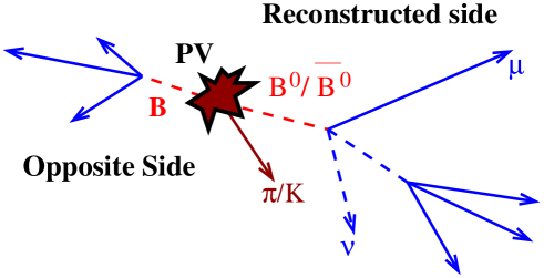
The meson flavor at its production can be identified using information
from the reconstructed side or from the opposite side
(see Fig. 1). One can tag the flavor using charge
correlation between “fragmentation tracks” associated with the
reconstructed meson. Such correlations were first observed in
events by the
OPAL experiment
sst . This is known as “same-side flavor tagging.”
The flavor can also be inferred from the decay information of the second
meson in the event, assuming that and are produced in pairs,
and thus in the ideal case, the two mesons have opposite flavors. This
method is known as “opposite-side flavor tagging.” An advantage of the latter
method is that its performance should be independent of the type of the
reconstructed meson.
Measurement of the mixing parameter is an important test of the
opposite-side flavor tagging as the same tagger is used for our study of
mixing. Studies of tagged and samples at hadron colliders
could reveal physics beyond the standard model berger .
Finally, this technique of flavor tagging developed at the Tevatron can also
be useful for future experiments at the Large Hadron Collider at CERN.
This paper describes the opposite-side flavor tagging algorithm used by the
DØ experiment in Run II and the measurement of its performance using
and events.
Throughout the paper,a reference to a particular final state also implies its
charge conjugated state. decays represent the main contribution to the
sample, and decays dominate in the
sample.
We measure the flavor tagging purity independently for reconstructed
and events and then extract the oscillation frequency.
This technique allows us to verify the assumption of independence of the
opposite-side flavor tagging on the type of reconstructed meson. Its
performance is described by the two parameters, efficiency and dilution.
The efficiency is defined as the fraction of reconstructed
events () that are tagged ():
(1)
The dilution is a normalized difference of correctly and wrongly tagged events:
(2)
where is called the purity. The
terms “correctly” and “wrongly” refer to the determination of the
reconstructed meson flavor. The effective tagging power of a
tagging algorithm is given by .
Figure 1:
Diagram of an event with a reconstructed candidate. PV indicates the primary vertex for the event.
II Detector Description
The DØ detector is described in detail elsewhere dzero .
The main features of the detector essential for this analysis are summarized below.
Tracks of charged particles
are reconstructed from the hits in the central tracking system, which consists of the
silicon microstrip tracker (SMT) and the central fiber tracker
(CFT), both located in a T superconducting solenoidal magnet.
The SMT has individual strips, with a typical pitch of
m and a design optimized for tracking and vertexing capability for
. The pseudorapidity, , approximates the
true rapidity, , for finite angles in
the limit of , being the polar angle.
We use the term “forward” to describe
the regions at large . The SMT system consists of six
barrels arranged longitudinally (each with a set of four layers of silicon
detectors arranged axially around the beam pipe), interspersed with 16 radial
disks. The CFT has eight thin coaxial barrels, each supporting two doublets of
overlapping scintillating fibers of 0.835 mm in diameter, one doublet being parallel
to the beam axis and the other alternating by relative to
this axis. Light signals are transferred via clear light fibers to solid-state
photon counters (VLPCs) that have quantum efficiency.
The muon system consists of a layer of tracking detectors
and scintillation trigger counters in front of T toroids,
followed by two additional similar layers after the toroids. Muon tracking for
relies on -cm-wide drift tubes,
while -cm mini drift tubes are used for .
Electrons are identified using matching between the tracks
identified in the central tracker and energy deposits in a
primarily liquid-argon/uranium sampling calorimeter dzero .
We also use the energy deposits in the central preshower detector dzero ,
which consists of three concentric cylindrical layers of triangular
scintillator strips and is located in a nominal 5 cm gap
between the solenoid and the central calorimeter, to provide
additional discrimination between electrons and fakes.
The calorimeter consists of the inner electromagnetic section
followed by the fine and coarse hadronic sections. In this analysis, we
only use the central calorimeter ().
III Data Sample and Event Selection
This measurement is based on a large semileptonic decay data
sample corresponding to approximately 1 fb-1 of integrated
luminosity collected with the DØ detector between April 2002 and October
2005.
mesons were selected using their semileptonic decays
and were divided into two exclusive groups: the sample,
containing all events with reconstructed decays,
and the sample, containing all the remaining events.
The sample is dominated by decays,
while the sample is dominated by decays.
The flavor tagging procedure was developed using events from the sample.
Events from the sample were used to measure the purity of the flavor tagging
and the oscillation
parameter . In addition, the purity was measured in the sample to test the hypothesis that the flavor tagger is independent of the type
of reconstructed meson.
Muons for this analysis were required to
have hits in more than one muon chamber, an associated track in the
central tracking system with hits in both SMT and CFT detectors, transverse
momentum GeV/, as measured in the central tracker,
pseudorapidity , and total momentum GeV/.
All charged particles in a given event were clustered into jets using the
DURHAM clustering algorithm durham with the cut-off parameter set to 15 GeV/. Events with more than one identified muon in the same jet or with
the reconstructed decays were rejected.
candidates were constructed from two tracks of opposite charge
belonging to the same jet as the reconstructed muon.
Both tracks were required to have transverse momentum GeV/ and
pseudorapidity .
They were required to form a common vertex with a
fit , number of degrees of freedom being 1.
For each track, the projection
(onto the axial plane, i.e. perpendicular to the beam direction) and projection
(onto the stereo plane, i.e. parallel to the beam direction)
of its impact parameter with respect to the
primary vertex, together with the corresponding uncertainties (,
) were computed.
The combined impact parameter significance
was required to be greater than 2.
The distance between the primary and vertices in the axial plane
was required to exceed 4 standard deviations: .
The accuracy of the determination was required to be better
than m. The angle between the momentum vector
and
the direction from the primary to the vertex in the axial plane was
required to satisfy the condition . The tracks of the
muon and candidate were required to form a common vertex
with a fit , with number of degrees of freedom being 1.
The mass of the kaon was assigned to the track having the same charge as
the muon; the remaining track was assigned the mass of the pion.
The mass of the
system was required to fall within the GeV/
range.
If the distance between the primary and vertices in the
axial plane exceeded , the angle between
the momentum and the direction from the primary to the vertex
in the axial plane was required
to satisfy the condition . The distance was
allowed to be greater than , provided that the distance between the
and vertices was less than .
The uncertainty was required to be less than m.
In addition, the cut GeV/ was applied.
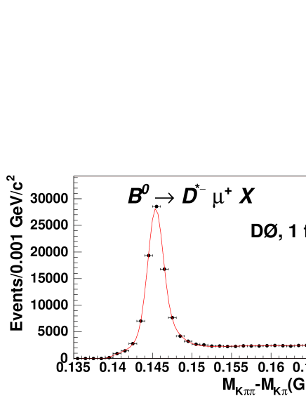
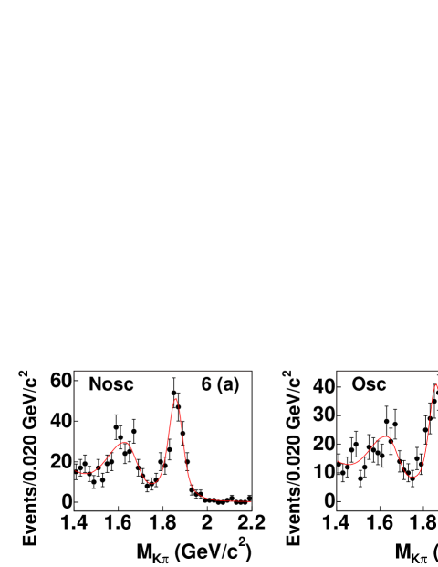
To select candidates, we searched for an additional pion track
with GeV/ and the charge opposite to the charge of the muon.
The mass difference for candidates, with GeV/, is shown
in Fig. 2. The peak corresponding to the mass of the
soft pion in the sample is clearly seen.
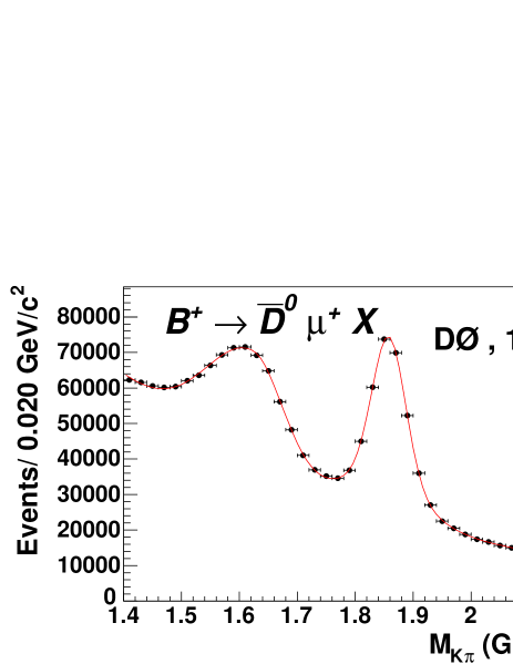
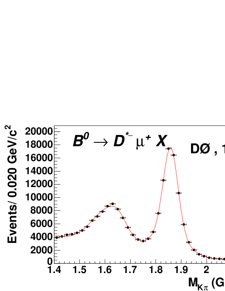
All events with GeV/ were included in the sample. The remaining events were assigned to the sample. The
mass distributions for these two samples together with the results of the fits
are shown in Figs. 3 and 4. The procedure to fit
these mass spectra is described in Sec.VII.
In total, decays
and decays
were reconstructed.
Figure 2:
The invariant mass distribution for selected candidates.
The curve shows the result of the fit described in Sec.VII.
Figure 3:
The invariant mass distribution for selected candidates.
The curve shows the result of the fit
described in Sec.VII.
Figure 4:
The invariant mass for selected candidates.
The curve shows the result of the fit described in Sec.VII.
IV Visible Proper Decay Length
The oscillations of mesons are usually
studied as a function of their proper decay
length. Since in semileptonic decays an undetected neutrino
carries away part of the energy, the proper decay length cannot be accurately measured.
Instead, a visible proper decay length (VPDL) was used in this analysis.
It is defined as
(3)
Here is a
vector in the plane perpendicular to the beam direction
from the primary to the meson decay vertex.
The transverse momentum is defined
as the vector sum of the transverse momenta of the muon and .
is the mass of meson.
V Description and combination of flavor taggers
Many different properties can be used to identify the initial flavor
or of a heavy quark fragmenting into a reconstructed meson.
Some of them have strong separation power, while others are
weaker. In all cases, their combination into a single tagging
variable gives a significantly better result than that in the case of
their separate use. We build such a combination
with the likelihood ratio method described below. We first describe
the combination algorithm and then discuss the discriminating
variables used.
V.1 Combination of variables
We construct a set of discriminating variables for a given event.
A discriminating variable,
by definition, should have different distributions for and flavors.
For the initial quark,
the probability density function (p.d.f.) for a given variable
is denoted as , while for the initial quark it is
denoted as . The combined tagging variable
is defined as:
(4)
A given variable may not be defined for some events. For example, there are
events that do not contain an identified muon on the opposite side.
In this case, the corresponding variable is set to 1.
An initial flavor is more probable if , and a
flavor is more probable if . By construction, an event
with is tagged as a quark and an event with is tagged as
a quark.
For an oscillation analysis, it is more convenient to define the tagging
variable as:
(5)
By construction, the variable which ranges between and .
An event with is tagged as a quark and with as a
quark, with higher values corresponding to higher tagging purities.
For uncorrelated variables , and perfect modeling
of the p.d.f., gives the best
possible tagging performance, and its absolute value provides a measure of
the dilution of the flavor tagging defined in Eqn. 2.
Very often, the analyzed events are divided into samples
with significantly different discriminating variables and
tagging performances.
This division would imply making a separate analysis for each sample
and combining the results at a later stage.
In contrast to this approach, the tagging variable defined by Eqs.
4 and 5
provides a “calibration” for all events, regardless of their intrinsic
differences. Since the absolute value of gives a measure of
the dilution of the flavor tagging, events from different categories
but with a similar absolute value of can be treated in the same way.
Thus, another important advantage of this method of flavor
tagging is the possibility of building a single variable having the same
meaning for different kinds of events. It allows us to
classify all events according to their tagging characteristics
and use them simultaneously in the analysis.
All of the discriminating variables used in this analysis
are constructed using the properties of the quark opposite to the reconstructed meson
(“opposite-side tagging”).
Since an important property of the opposite-side tagging is the independence
of its performance of the type of reconstructed meson,
it can be calibrated
in data by applying tagging to the events with and decays.
The measured performance can then be used to study meson oscillations,
as an example.
The probability density functions for each discriminating variable
discussed below were constructed using events from the sample with
m.
In this sample, the decay
dominates, see Sec. VII.3.
The events give a 16% contribution
to the sample and, due to the cut on VPDL, contains mainly non-oscillated decays, as determined by Monte Carlo (the standard pythia
generation, followed by decay of B mesons with EvtGen, passed through
Geant and then reconstruction).
The initial flavor of a quark is therefore determined by the charge
of the muon. Estimates based on Monte Carlo simulation indicate that
the purity of the initial flavor determination in the selected sample is
, where the uncertainty is due to the uncertainties in
measured branching fractions of meson decays.
For each discriminating variable,
the signal band containing all events
with and the background band
containing all events with were defined.
The p.d.f’s were constructed as the difference in the distributions. The
latter distributions were normalized by multiplying them by 0.74
so that the number of events in the background band corresponds to the
estimated number of background events in the signal band.
V.2 Flavor tagger discriminants
We now describe the variables used.
An additional muon was searched for in each analyzed event. This muon
was required
to have at least one hit in the muon chambers
and to have ,
where is the three-momentum of the reconstructed meson,
and is the angle between the vectors and
.
If more than one muon was found, the muon with the
highest number of hits in the muon chambers was used. If more than
one muon with the same number of hits in the muon chambers was found,
the muon with the highest transverse momentum was used.
For this muon, a muon jet charge was constructed as
where is the charge and is the transverse momentum
of the ’th particle, and
the sum is taken over all charged particles, including the muon,
satisfying the condition
,
where and are computed with respect to
the muon direction. Daughters of the reconstructed meson
were explicitly excluded from this sum. In addition, any charged particle
with was excluded.
The distribution of the muon jet charge variable
is shown in Figs. 5(a) and (b).
In these plots, gives
the charge of the quark in the reconstructed
decay, in this case given
by the muon charge.
We build separate p.d.f.’s for muons with hits in all
three layers of the muon detector, Fig. 5(a), and for
muons with fewer than three hits, Fig. 5(b).
In addition to the muon tag, reconstructed electrons with were also used for flavor tagging.
The electron is reconstructed by extrapolating a track to the calorimeter and adding up the energy deposited in a narrow tube or “road” around the track. Calorimeter cells
are collected around the track extrapolated positions in each layer
and the total transverse energy of the cluster is defined by the sum of the
energies in each layer. The electrons are required to be in the central region
(), with GeV/c. They are required to have at
least one hit each in the CFT and SMT. They are required to have energy deposits
in the EM calorimeter consistent with an electron,
, and low energy deposit in the hadron calorimeter, . The cuts are looser for electrons with and are given
in brackets. and are calculated as below:
(6)
(7)
where is the transverse energy within the road in the ’th layer.
We also require a minimum single layer cluster energy of a cluster
in the central preshower, MeV/c.
The cuts were optimized by studying electrons from conversion decays () and fakes from decays to obtain a purity for electrons.
For these electrons, an electron jet charge () was constructed in
the same way as the muon jet charge, .
The distribution of the electron jet charge variable
is shown in Fig. 5(c).
Figure 5:
(a) Distribution of the jet charge for muons with hits in all
three layers of the muon detector.
(b) Distribution of the jet charge , for muons with fewer than three hits.
(c) Distribution of the jet charge for electrons . Here
is the
charge of the muon from the reconstruction side.
An additional secondary vertex corresponding to the decay of a hadron
was searched for, using all charged tracks in the event
excluding those from the reconstructed hadron.
The secondary vertex was also required to contain at least two tracks with an
axial impact parameter significance greater than 3. The distance from
the primary to the secondary vertex must also satisfy the condition:
. The details of the secondary vertex
identification algorithm can be found in Ref. pvreco .
The three-momentum of the secondary vertex is defined
as the vector sum of the momenta of all tracks included in the secondary vertex.
A secondary vertex with was
used for flavor tagging.
A secondary vertex charge is defined as the third
discriminating variable
where the sum is taken over all tracks included in the secondary vertex.
Daughters of the reconstructed meson were explicitly excluded
from this sum. In addition, any charged particle
with was excluded.
Here is the longitudinal momentum of track with respect to
the direction of the secondary vertex momentum pV.
A value of was used, taken from previous studies
at LEP delphi . We verified that this value of results in the optimal
performance of the variable.
Figures 6(a) and 6(b) show the distribution
of this variable for the events with and without an identified muon flavor tag.
Finally, the event charge was constructed as
The sum is taken over all charged tracks with
and having .
Daughters of the reconstructed meson were explicitly excluded
from this sum.
The distribution of this variable is shown in Fig. 6(c).
For each event with an identified muon, the muon jet charge
and the secondary vertex charge were used to construct
a muon tagger. For each event without a muon but with an identified electron,
the electron jet charge and the secondary vertex charge were used to construct
an electron tagger. Finally, for events without a muon or an electron but with a reconstructed
secondary vertex, the secondary vertex charge
and the event jet charge were used to construct
a secondary vertex tagger. The resulting distribution
of the tagging variable for the combination of all three taggers,
called the combined tagger, is shown in Fig. 7.
The performances of these taggers are discussed in the following sections.
Figure 6:
(a) Distribution of the secondary vertex charge for events with an opposite-side muon.
(b) Distribution of the secondary vertex charge for events without an opposite-side muon.
(c) Distribution of the event jet charge.
is the
charge of the quark from the reconstruction side.
Figure 7:
Normalized distributions of the combined tagging variable.
is the
charge of the quark from the reconstruction side.
VI Multidimensional Tagger
In addition to the flavor tagger described in Sec. V,
an alternative
algorithm was also developed and used to measure mixing.
This tagger
is multidimensional, i.e., the likelihood functions it is
based on depend on more than a single variable.
In addition, the p.d.f.’s were determined from simulated events,
while the primary flavor tagger described in Sec.V
uses data to construct the p.d.f.’s. The multidimensional tagger
therefore provides a cross-check of the primary algorithm.
If, as before, we have a set of discriminants ,
the likelihood that the meson has flavor
at the time of creation can be written as .
A similar expression holds
for the likelihood for . These
likelihoods relate to the variable as
The likelihoods are obtained from the simulated samples
of with . This final state does not oscillate and is therefore
flavor-pure. The sample was used
to obtain , while was determined
from sample.
In practice, the likelihoods
were stored as multidimensional histograms (with one dimension per discriminating
variable) with the bin content normalized to the total number of events
in the sample. For a given event, the tagger output was obtained
by substituting the appropriate normalized bin contents
into Eq. (8).
In addition to the discriminating variables introduced in Sec.V,
other variables were used for the multidimensional tagger.
For each identified opposite-side muon, the
transverse momentum relative to the beam axis and
transverse momentum relative to the nearest jet were computed.
(The muon was included in the jet clustering.)
Another variable defined for the muon is its impact parameter significance
, where is the transverse impact parameter significance , where is defined in Sec. III.
For each reconstructed opposite-side secondary
vertex, the secondary vertex transverse momentum was computed by
taking the magnitude of the transverse projection of the vector sum of all tracks
in that vertex.
In principle, all discriminating variables
can be combined into a single multidimensional likelihood.
However, since a binned likelihood was used, in order to achieve a reasonable
resolution in any given discriminant, the binning
must be fine enough to resolve its useful features.
In practice, because of limited simulation statistics, this
means that discriminating variables must be chosen wisely
when making a combination.
All events were divided into three categories based on their opposite-side
content. The following variables for different categories
were selected.
1.
Events with muon and secondary vertex:
Tag(SV)=.
2.
Events with muon and without secondary vertex.
Tag(SV)=.
3.
Events with secondary vertex without a muon:
Tag(SV)=.
Distributions in the tagging variable for the above three taggers
are shown in Fig. 8. They were
made by applying the taggers to the simulated
samples from which they were created.
The final multidimensional tagger used the following logic to
decide which of its sub-taggers to use.
For events containing a muon and a secondary vertex, the Tag(SV)
was used. If the opposite side contained a muon and no secondary vertex,
the Tag(SV) was used.
If the opposite side contained an electron, the electron tagger
described in Sec. V was used.
Note that this tagger is not multidimensional
and is not derived from simulation.
If the opposite side contained a secondary vertex, the Tag(SV)
was used.
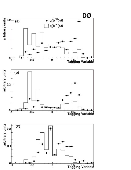
Figure 8:
Normalized distributions of the combined tagging variable
for three multidimensional taggers for the simulated samples
.
Here is the charge of the quark from the reconstructed side.
(a) Distribution of for Tag(SV).
(b) Distribution of for Tag(SV).
(c) Distribution of for Tag(SV).
VII Asymmetry Fit Procedure
The performance of the flavor tagging and measurements of the mixing
frequency were obtained from a study of the dependence of the flavor
asymmetry on the -meson decay length.
The flavor asymmetry is defined as:
(9)
Here is the number of non-oscillated decays and
is the number of oscillated decays.
An event with
was tagged as non-oscillated,
and an event with
was tagged as oscillated.
The flavor tagging variable is defined in Eq. (5)
or (8).
All events in the and samples were divided into seven groups
according to the measured VPDL () defined in Eq. (3).
The numbers of oscillated and
non-oscillated signal events in each group were
determined from the number of the signal events given by a fit
to the invariant mass distribution for both samples.
The seven VPDL bins (in cm) defined were:
, , , , , and .
VII.1 Mass Fit
In this section we describe the mass fitting procedure.
The fitting function was chosen to give the best of the fit to
the mass spectrum of the entire sample of
events shown in Figs. 3 and 4. The signal
peak corresponding to the decay can be seen
at 1.857 GeV/. The background to the right of the signal region is adequately
described by an exponential function:
(10)
where is the mass.
The peak in the background to the left of the signal is due to
events in which mesons decay to where
is not reconstructed.
It was modeled with a
bifurcated Gaussian function:
Here
is the mean
of the Gaussian, and and are the two widths
of the bifurcated Gaussian function.
The signal has been modeled by the sum of two Gaussians:
(12)
where is the number of signal events,
and are the means of the Gaussians,
and are the widths of the Gaussians,
and is the fractional contribution of the first Gaussian.
The complete fitting function, which has twelve free parameters, is:
(13)
The low statistics in some VPDL bins,
which have as few as ten events after flavor tagging,
do not permit a free fit to this function,
Consequently some parameters had to be constrained or fixed. In order to do this,
it was necessary to
show that the constraints on the parameters are valid for all of the VPDL
bins. Unconstrained fits were performed to several high statistic samples, and
the set of all events was used as a reference fit. Events were divided into
VPDL bins and fit to investigate the VPDL dependance of the fit results.
In addition, three
samples were made to test whether the presence of a flavor
tag changes the mass spectrum: all tagged events over the entire
VPDL range, all events in the short VPDL range [0,0.05] tagged
as opposite-sign events, and all events in VPDL range
[0,0.05] tagged as same-sign events.
This study showed that the width, position, and the ratio of the signal
Gaussians, as well as the position and widths of the bifurcated
Gaussian describing the background can be fixed
to the values obtained from the fit to the
total or mass distribution.
This left four free parameters: the
numbers of events in the signal peak, background peak, and
exponential background, and the slope constant of the exponential
background.
Examples of the fits to the mass distribution in different
VPDL bins are shown in Fig. 9.
The number of candidates was estimated using the distribution of
,
shown in Fig. 2.
In this case, the signal was modeled with two Gaussians as described by
Eq.(12), and the background
by the product of a linear and exponential function
(14)
where is the mass difference in this equation.
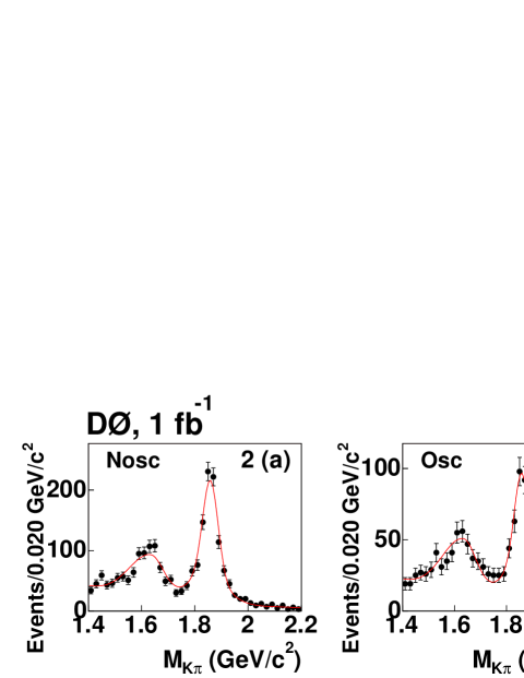
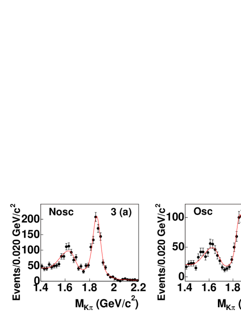
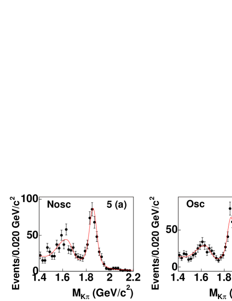
Figure 9: The fit to mass for non-oscillating (left) and
oscillating (right) events tagged by
the muon tagger with in VPDL bins
cm (2a,2b),
cm (3a,3b),
cm (5a,5b),
and, cm (6a,6b).
VII.2 Expected flavor asymmetry
For a given type of meson (), the distribution of the
visible proper decay length is given by
(15)
(16)
(17)
(18)
(19)
(20)
Here is the lifetime of the meson, is the mixing frequency
of mesons, the factor
reflects the difference between the measured ()
and true () momenta of the meson.
The meson does not oscillate, and it is assumed in these studies that
the meson oscillates with infinite frequency.
The flavor tagging dilution is given by . In general, it can be different for and . In our study we verified the
assumption that for our opposite-side flavor tagging.
The transition from the true to the experimentally measured visible
proper decay length is achieved by integration
over the -factor distribution and convolution with the resolution function:
(21)
Here is the detector resolution in the VPDL, and
is the reconstruction efficiency for a given channel
of meson decay. The step function forces to be positive
in the integration. can be negative due to resolution effects.
The function is a normalized distribution of the -factor
in a given channel , obtained from simulated events.
In addition to the main decay channel , the process
contributes to the selected final state.
A dedicated analysis was developed to study this process, both in data and in simulation.
It shows that the pseudo decay-length, constructed from
the crossing of the and trajectories, is distributed around zero
with m. The distribution of the VPDL
for this process was taken from simulation. It was assumed
that the production ratio is the same as in semileptonic
decays and that the flavor tagging for the events gives the
same rate of oscillated and non-oscillated events. The fraction
of events was obtained from the fit.
Taking into account all of the above mentioned contributions,
the expected number of (non-) oscillated events in the -th bin of VPDL is
(22)
Here the integration is taken over a given interval ,
the sum is taken over all decay channels
contributing to the selected sample,
and is the branching fraction of channel .
Finally, the expected value of asymmetry, , for the interval of the measured VPDL is given by
(23)
The expected asymmetry can be computed both for the and the samples.
The only difference between them is due to the different relative contributions of various decay channels of mesons.
For the computation of , the meson lifetimes and
the branching fractions were taken from the Particle Data Group (PDG) pdg .
They are discussed in the following section. The functions , ,
and were obtained from MC simulation. Variations of these inputs
within their uncertainties are included in the systematic uncertainties.
VII.3 Sample Composition
There is a cross-contamination between the , ; and samples.
To determine the composition of the selected samples, we studied all possible decay chains for , , and with their corresponding branching fractions, from which we estimated the sample composition in the and samples.
The following decay
channels of mesons were considered for the sample:
and for the sample:
Here, and in the following, the symbol “” denotes both narrow
and wide resonances, as well as non-resonant
and production.
The most recent PDG values pdg were used to
determine the branching fractions of decays
contributing to the and samples:
Br
was estimated using the following inputs:
(24)
where is the lifetime, and is the lifetime.
The following value was obtained:
(25)
is obtained as follows:
Br
was estimated from the following inputs:
and assuming Brpdg . The usual practice in estimating this decay rate is to neglect
the contributions of the decays . However, the above data allows us to take these decays into account.
Neglecting the decays ,
the available measurements can be expressed as:
From these relations and using the above measurements, we obtain
(26)
All other factors for the
were obtained assuming the following relations,
was estimated
from the following inputs:
To estimate branching fractions for decays,
was taken
from Ref. pdg and the following assumptions were used:
where is the meson lifetime. In addition, it was assumed that
(27)
There is no experimental measurement of this ratio yet and to estimate the
the corresponding systematic uncertainty, this ratio was varied between
0 and 1.
In addition to these branching fractions,
various decay chains are affected differently by the
meson selection cuts, and
the corresponding reconstruction efficiencies were determined from
simulation to correct for this effect.
Taking into account these efficiencies, the composition of the
sample was estimated to be ,
, and . The sample contains
, , and .
Since the sample was selected by the cut on the mass difference
, there is a small
additional contribution
of events to the sample, when is randomly combined with a pion from the combinatorial background.
The fraction of this contribution was estimated using events.
These events were selected applying all the criteria for the sample,
described in Sec. III, except that the
wrong charge correlation of muon and pion was required, i.e., the
muon and the pion were required to be having the same charge.
The number of events was determined using the same fitting procedure
as for the sample, and the additional fraction of
events in the sample was estimated to be .
This fraction was included in the fitting procedure and
the uncertainty in this value was taken into account in the overall systematics.
VIII Results
For each sample of tagged events, the observed and expected asymmetries
were determined using Eqs. (9) and (23) in all VPDL bins,
and the values of , , , and
were obtained from a simultaneous fit:
(28)
(29)
(30)
Here is the sum over all VPDL bins.
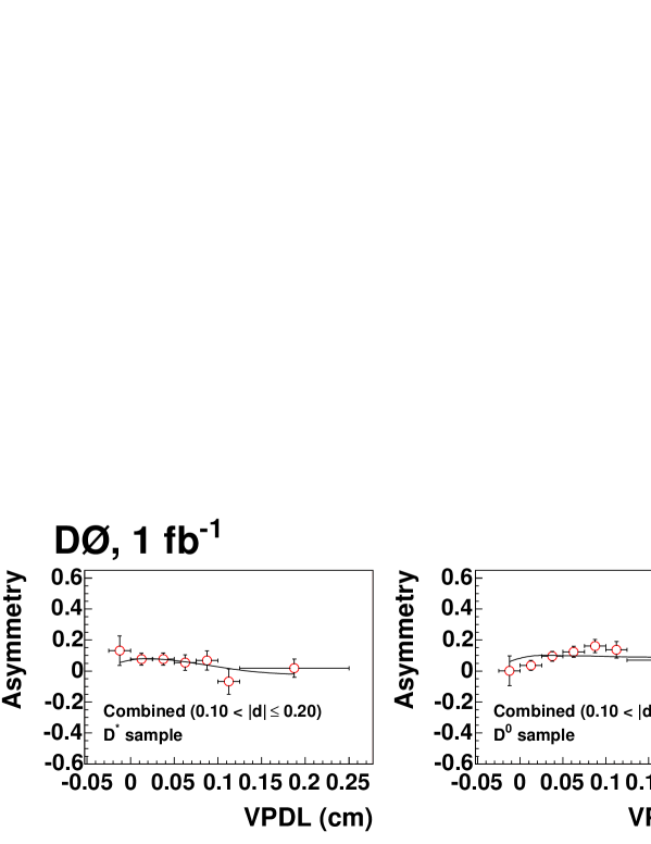
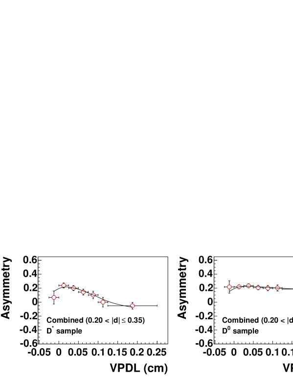
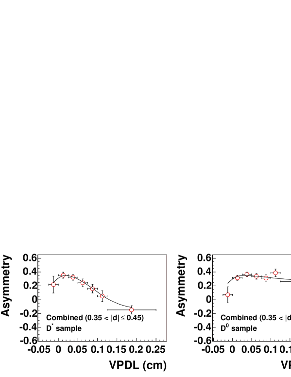
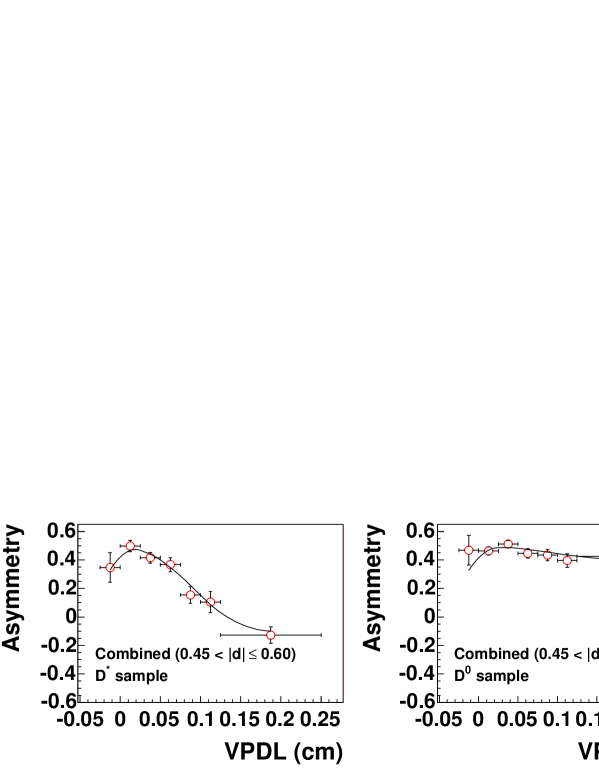
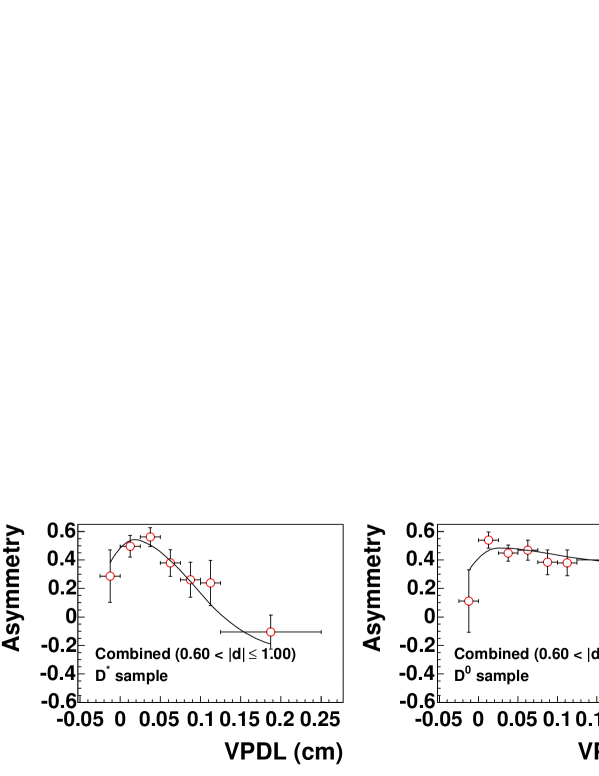
Examples of the fit to the flavor asymmetry minimization given
in Eq. (VIII), is shown in Fig. 10.
Figure 10: Asymmetries obtained in the and sample with the
combined tagger in bins.
Circles are data, and the result of the fit
is superimposed.
The performance of the flavor tagging method was studied
separately for the muon, electron, and secondary vertex taggers
using events with . Results
are given in Tables 1–3. All uncertainties in these
tables are statistical only and do not
include systematic uncertainties. The performances of the combined
tagger defined in Sec.V.2 for events with
and the alternative multidimensional tagger defined in Sec.VI
for events with are also shown. The cut on is somewhat
different for the multidimensional tagger as the calibration is different
and we compare the dilutions for the same tag efficiency for the two taggers.
The tagging efficiencies shown in Tables 1 and 2
were computed using events with VPDL=[0.025,0.250]. This selection
reduces the contribution from events,
since they have a VPDL distribution with zero mean and m
as described in Sec.VII.
Table 1:
Tagging performance for the sample for different taggers and subsamples. Uncertainties
are statistical only.
Tagger
Muon ()
Electron ()
SVCharge ()
Combined ()
Multidim. ()
Combined (0.100.20)
Combined (0.200.35)
Combined (0.350.45)
Combined (0.450.60)
Combined (0.601.00)
Table 2:
Tagging performance for the sample for different taggers and subsamples.
For comparison, the dilution measured in the sample
with addition
of wrong sign events is also shown. Uncertainties are statistical
only.
Tagger
Muon ()
Electron ()
SVCharge ()
Combined ()
Multidim. ()
Combined (0.100.20)
Combined (0.200.35)
Combined (0.350.45)
Combined (0.450.60)
Combined (0.601.00)
Table 3:
Measured value of and for different taggers
and subsamples.
Tagger
(ps-1)
Muon
Electron
SVCharge
Multidim.
Combined ()
Combined ()
Combined ()
Combined ()
Combined ()
Combined ()
Individual taggers give compatible values of
and , as can be seen in Table 3.
For the combined tagger with , the following results were
obtained:
(31)
The multidimensional tagger which used simulation for the description
of p.d.f.’s as described in Sec.VI gives
consistent results both for the and the fraction ,
which is used as a cross-check of the main tagging algorithm.
One of the goals of this analysis was to verify the assumption
of independence of the opposite-side flavor tagging on the type of the
reconstructed meson. It can be seen from Tables 1 and 2
that the measured flavor tagging performance for events is slightly
better than for events, both for individual and combined taggers.
This difference can be explained by the better selection of
events due to an additional requirement of the charge correlation between the
muon and pion from decay. The
sample can contain events with a wrongly selected muon. Since the
charge of the muon determines the flavor asymmetry, such
a background can reduce
the measured dilution. The charge correlation between
the muon and the pion suppresses this background and results in a
better measurement of the tagging performance.
To verify this hypothesis, a special sample of events satisfying all conditions
for the sample, except the requirement of the charge correlation between
the muon and the pion, was selected. The dilution for this
sample is shown in Table 2. It can be seen that
is systematically lower than for all samples and all taggers.
is the right quantity to be compared with and
Table 2 shows that they are statistically compatible.
This result therefore confirms the expectation of the same performance
of the opposite-side flavor tagging for and events.
It also shows that contribution of background
in the sample reduces the measured dilution for events.
Thus, the dilution measured in the sample can be used for the
mixing measurement, where a similar charge correlation between
the muon and is required.
By construction, the dilution for each event
should strongly depend on the magnitude of the tagging variable .
This property becomes important in the mixing measurement,
since in this case the dilution
of each event can be estimated using the value of and
can be included in a likelihood function, improving
the sensitivity of the measurement.
To test the dependence of the dilution on ,
all tagged events were divided into subsamples with
, , ,
, and . The overall tagging efficiency
for this sample is . The dilutions obtained
are shown in Table 1. Their strong dependence on the value
of the tagging variable is clearly seen. This allows us to perform
a dilution calibration and obtain the measured dilution as a function
of the predicted value . This is used to provide an event-by-event
dilution for the mixing analysis and the calibration derived
in this analysis is used for the two sided C.L. on mixing, obtained
by DØ bsd0 . The overall tagging power,
computed as the sum of the tagging powers in all subsamples, is:
(32)
The measured oscillation parameters for all considered taggers and
subsamples are given in Table 3.
They are compatible with the world average value
ps-1pdg in each instance.
The final mixing parameter was obtained from the simultaneous
fit of the flavor asymmetry in the various tagging variable subsamples
defined above.
The fraction was constrained to be the same for all subsamples.
The result is
(33)
The statistical precision of from the simultaneous fit is about
10% better than that from the fit of events with .
This improvement is directly related to a better overall tagging power
[Eq. (32)] for the sum of subsamples as compared to the result
[Eq. (VIII)] for the sample with .
IX Systematic Uncertainties
The systematic uncertainties are summarized in
Tables 4 and 5.
Table 4 shows the
contributions to the systematic uncertainty in .
Table 5 shows the corresponding contributions to the systematic
uncertainties in .
Table 4: Systematic uncertainties for .
Default
Variation
(ps
(a)
(b)
(a)
(b)
5.44
0.002
0.002
1.07
0.17
0.17
0.0078
0.0078
0.35
0
1.0
0.0006
0.0012
lifetimes
0.05022
0.00054
0.00054
0.0008
0.0008
Resolution scale factor
—
1.2
0.8
0.0021
0.0021
Alignment
—
m
m
0.004
+0.004
-factor
—
2%
+2%
0.0098
0.0094
Efficiency
—
12%
+12%
0.0054
0.0052
Fraction in
4%
3.15%
4.85%
0.0020
+0.0030
Fit procedure
See below
Bin width
2 MeV
1.6
2.67
0.0009
0.0014
Parameter
—
0.0001
0.0001
Parameter
—
0.0001
—
Parameter
—
0.0001
0.0001
Parameter
—
0.0016
0.0015
Parameter
—
0.0006
0.0006
Parameter
—
.0005
0.0004
Parameter
—
0.0006
0.0007
Parameter
—
—
—
Fit procedure
Overall
+0.0023
0.0019
Total
Table 5: Systematic uncertainties for .
Default
Variation
(a)
(b)
(a)
(b)
(a)
(b)
(a)
(b)
(a)
(b)
(a)
(b)
5.44
0.23
0.23
—
—
—
0.001
0.001
—
0.001
0.001
0.001
0.001
1.07
0.17
0.17
0.0004
0.0004
0.0011
0.0011
0.0019
0.0021
0.0020
0.0021
0.0008
0.0028
0.35
0.0
1.0
0.0009
0.0016
0.0027
0.0048
0.0042
0.0079
0.0057
0.0105
0.0066
0.0124
lifetimes
0.05022
0.00054
0.00054
—
0.0001
0.0001
0.0002
0.0003
0.0001
0.0003
0.0003
0.0014
0.0003
Resolution function
—
1.2
0.8
0.0005
0.0006
0.0010
0.0012
0.0020
0.0021
0.0024
0.0028
0.0028
0.0032
Alignment
—
10
10
0.004
0.004
0.004
0.004
0.004
0.004
0.004
0.004
0.004
0.004
-Factor
—
2%
+2%
—
—
0.0001
—
—
0.0001
0.0001
—
—
—
Efficiency
—
12%
+12%
0.0006
0.0007
0.0008
0.0006
0.0012
0.0011
0.0013
0.0010
0.0021
0.0019
Fraction in
4%
3.15%
4.85%
—
0.0010
0.0010
—
0.0010
0.0010
0.0010
0.0010
0.0010
0.0010
Fit procedure
See split below
Bin width
2 MeV
1.6
2.67
0.0026
0.0002
0.0024
0.0014
0.0001
0.0027
0.0037
0.0038
0.0089
0.0087
Parameter
—
0.0003
0.0002
0.0001
0.0001
0.0001
0.0001
0.0002
0.0001
0.0007
0.0007
Parameter
—
0.0002
0.0002
0.0001
0.0001
0.0004
0.0003
—
0.0001
0.0002
0.0001
Parameter
—
0.0005
0.0005
0.0002
0.0001
0.0002
0.0001
0.0002
0.0001
0.0015
0.0011
Parameter
—
-
0.0009
0.0010
0.0017
0.0018
0.0023
0.0015
0.0006
0.0005
0.0004
0.0004
Parameter
—
0.0008
0.0005
0.0014
0.0009
0.0037
0.0034
0.0013
0.0017
0.0099
0.0068
Parameter
—
0.0015
0.0011
0.0029
0.0024
0.0030
0.0027
0.0013
0.0011
0.0046
0.0035
Parameter
—
—
0.0003
0.0008
0.0011
0.0001
0.0006
0.0003
0.0002
0.0008
0.0003
Parameter
—
0.0001
—
0.0004
0.0003
0.0002
0.0002
0.0004
0.0004
0.0006
0.0010
Fit procedure
Overall
+0.0021
+0.0040
+0.0060
+0.0044
+0.0119
0.0031
0.0041
0.0046
0.0019
0.0111
Total
+.0049
+.0077
+.0111
+.0125
+.0182
0.0052
0.0066
0.0081
0.0081
0.0140
These uncertainties were obtained as follows:
•
The meson branching fractions and lifetimes used in the fit of the
asymmetry were taken from Ref. pdg and were varied by one standard deviation.
•
The VPDL resolution obtained in simulation was multiplied by
factors of 0.8 and 1.2. These factors exceed the uncertainty
in the difference of the resolution between data and simulation.
•
The variation of -factors with the change in the momentum
was neglected in this analysis. To check the impact of this assumption on the
final result, the computation of -factors, was repeated without the cut
on or by applying an additional cut on the of muon,
GeV/. The change in the average values of the -factors did not
exceed 2%, which was used as the estimate of the systematic uncertainty in their values. This uncertainty was propagated into the variation of
and tagging purity by repeating the fit with the -factor distributions
shifted by 2%.
•
The ratio of the reconstruction efficiencies in different meson decay channels
depends only on the kinematic properties of corresponding decays and
can therefore be reliably estimated in the simulation. The ISGW2
model isgw2 of semileptonic decays was used. The
uncertainty in the reconstruction efficiency, set at 12%, was
estimated by varying the kinematic cuts on the of the muon and
in a wide range. Changing the model describing semileptonic
decay from ISGW2 to a HQET-motivated model hqet produces a smaller
variation. The fit to the asymmetry was repeated with the efficiencies
to reconstruct the and channels modified by , and the difference was taken
as the systematic uncertainty from this source.
•
The additional fraction of events contributing to the sample
was estimated at (see Sec. VII.3).
This variation was used to estimate the systematic uncertainty from this source.
As a cross-check, the number of events was determined from the fit
of the mass difference and the fit
of the flavor asymmetry was repeated. The measured value of
ps-1 is consistent with Eq. (33).
•
We also investigated the systematic uncertainty in determining the
number of and candidates in each VPDL bin.
–
The values of the parameters which had been fixed from the fit to “all” events,
were varied by .
–
The default bin width for the fits in the VPDL bin is 0.020 GeV. We
lowered the bin width to 0.016 GeV and increased the bin width to
0.027 GeV, and included the resulting variations in the systematic uncertainty.
X Conclusions
We have performed a study of a likelihood-based opposite-side tagging
algorithm in and samples obtained with fb-1 of
RunII Data.
The dilutions and were found to be
the same within their statistical uncertainties. This result justifies
the application of the dilution to the mixing analysis.
Splitting the sample into bins according to the
tagging variable and measuring the tagging power as
the sum of the individual tagging powers of all bins, we obtained a tagging power of
From the simultaneous fit to events in all bins we measured the
mixing parameter:
which is in good agreement with the world average value of
pdg .
We thank the staffs at Fermilab and collaborating institutions,
and acknowledge support from the
DOE and NSF (USA);
CEA and CNRS/IN2P3 (France);
FASI, Rosatom and RFBR (Russia);
CAPES, CNPq, FAPERJ, FAPESP and FUNDUNESP (Brazil);
DAE and DST (India);
Colciencias (Colombia);
CONACyT (Mexico);
KRF and KOSEF (Korea);
CONICET and UBACyT (Argentina);
FOM (The Netherlands);
PPARC (United Kingdom);
MSMT (Czech Republic);
CRC Program, CFI, NSERC and WestGrid Project (Canada);
BMBF and DFG (Germany);
SFI (Ireland);
The Swedish Research Council (Sweden);
Research Corporation;
Alexander von Humboldt Foundation;
and the Marie Curie Program.
References
(1)
On leave from IEP SAS Kosice, Slovakia.
(2)
Visitor from Helsinki Institute of Physics, Helsinki, Finland.
(3) H. Albrecht et al., ARGUS Collaboration, Phys. Lett. B 192,
245 (1987); M. Artuso et al., CLEO Collaboration, Phys Rev. Lett. 62, 2233 (1989).
(4) R. Akers et al., OPAL Collaboration, Z. Phys. C 66, 19 (1995).
(5)
S. Eidelman et al., Particle Data Group, Phys. Lett. B
592, 1 (2004).
(6) E. Berger et al., Phys. Rev. Lett. 86, 4231 (2001).
(7) V.M. Abazov et al., DØ collaboration,
Nucl. Instrum. and Methods A 565, 463-537 (2006).
(8) S. Catani et al., Phys. Lett. B 269, 432 (1991).
(9) J. Abdallah et al., DELPHI Collaboration,
Eur. Phys. J. C32, 185 (2004).
(10) J. Abdallah et al., DELPHI Collaboration, Euro. Phys. J. C35, 35 (2004).
(11)
D. Scora and N. Isgur, Phys. Rev. D 52, 2783 (1995).
(12) M. Neubert, Phys. Rep. 245, 259 (1994).
(13)
D. Buskulic et al., ALEPH Collaboration, Z. Phys. C 73, 601 (1997).
(14)
P. Abreu et al., DELPHI Collaboration, Phys. Lett. B
475, 407 (2000).
(15) V. M. Abazov et al., DØ Collaboration, Phys. Rev. Lett. 97, 021802 (2006).