Finding The Charm In 800 GeV/c
p-Cu  and p-Be  Single Muon Spectra
By

Stephen A. Klinksiek
B.S., Physics/Mathematics, New Mexico Highlands University, 1993    
             M.S., Physics, University of New Mexico, 1999   
DISSERTATION
Submitted in Partial Fulfillment of the
Requirements for the Degree of
Doctor of Philosophy
Physics
University of New Mexico
Albuquerque, New Mexico

December, 2005

©2005, Stephen A. Klinksiek

Dedication

To Isabella

Acknowledgments

Some dreams do come true.

This has been a long, hard and at times dark and dreary road to travel, especially for someone my age from a small town in Northern New Mexico. I couldn’t do it alone, and there are many who need to know that, without their support and belief in me, it wouldn’t have happened. They were the luminarias to guide me through.

I have had the incredible fortune to meet and know two true gentlemen along the way, Bernd Bassalleck and Jim Lowe. I don’t use the word ’gentleman’ lightly. That you ever put up with me is testimony to your kindness and generosity. Now all I have to do is figure out how to repay you. Muchos gracias.

A special note for the one who got this started, Doug Fields. How did Bernd put it? ”Glad it aint my dissertation!” As bad as it seemed to get, you helped make it happen. Thank you. Then there is Tim Thomas. You never let me feel that I couldn’t get it done. Students everywhere are missing the chance to learn from Paul Reimer.

To mom, Norm, Albert and Rachel. No one ever had better parents. Dad, Richard and Susan, I wish you could be here.

That leaves the most important person in my life, Elizabeth. I dedicated this to you, and now I thank you. You stuck with me through thick and thin, and I love you more than ever for it.

Finding The Charm In 800 GeV/c
p-Cu  and p-Be  Single Muon Spectra
By

Stephen A. Klinksiek

ABSTRACT OF DISSERTATION
Submitted in Partial Fulfillment of the

Requirements for the Degree of

Doctor of Philosophy

Physics

University of New Mexico

Albuquerque, New Mexico

December, 2005

Fermilab Experiment 866 took single muon data from 800 GeV/c ($\sqrt{s}=38.8$ GeV) p-Cu  and p-Be  interactions in an attempt to extract the inclusive nuclear open charm/anti-charm ($D/\overline{D}$) differential cross sections as a function of $p_{T}$. The muons were decay products from semi-leptonic decays of open charm mesons as well as decays from lighter non-charmed mesons ($\pi$’s and K’s). Data were taken simultaneously from two interaction regions; one of two thin nuclear targets and a copper beam dump 92 inches downstream. The open decay length for hadrons produced in the targets increased the contribution to the muon spectrum from light hadron decays, relative to those from the dump. Production cross sections for light hadrons from previous experiments were used in conjunction with parameterized open charm cross sections to produce total Monte Carlo single muon spectra that were subsequently fit to the data.

The sensitivity of this measurement covered an open charm hadron $p_{T}\;$range of approximately 2 to 7 GeV/c, center-of-mass rapidity, $y_{cm}$, between 0 and 2, and $x_{F}$ between 0.2 and 0.8. Previous experimental results for p-p  or p-A  open charm production at comparable energy was limited to $\sqrt{5}$ GeV/c. Three functions describing the shape of the open charm/anti-charm cross sections were fit to the data; an exponential, $A_{1}\,exp\left(-B\,p_{T}\right)$, and two polynomials, $\frac{A_{2}}{\left(p_{T}^{2}+\alpha\,m_{c}^{2}\right)^{n}}\;$and $A_{2}\,\frac{\left(1-p_{T}\,/\,p_{beam}\right)^{m}}{\left(p_{T}^{2}+\alpha\,m_{c}^{2}\right)^{n}}$. The first polynomial was fit with the parameter $n$ as a free parameter, and constant with three integer values, 4, 5 and 6. The second was fit with $n$ held fixed at the constant integer values only. The best results were with the first polynomial with $n$ around 6. All three parameterizations resulted in good fits. Extrapolation of the cross sections to small $p_{T}\;$shows good agreement with previous experiments. The power $\alpha$ of the nuclear dependency $A^{\alpha(p_{T})}$ was calculated as a function of $p_{T}$. The result indicates that $\alpha$ is transverse-momentum dependent, albeit within large errors.

Contents

toc

List of Figures

lof

List of Tables

lot

Chapter 1 Introduction

Quantum Chromo-Dynamics (QCD), and the Standard Model (SM) as a whole, have been remarkably successful in describing the nature of particles and their interactions. They are widely accepted by the community. The Standard model is composed of six quarks (referred to as flavors), six leptons and four force carriers, neglecting gravity. Quarks and leptons come in three generations. A quark generation consists of two quarks, one having charge $+\,2\,/\,3$ and one having charge $-\,1\,/\,3$. The quarks also come in three colors, red, green and blue. Each generation of leptons consists of a pair with one neutral and the other having unit charge. Quarks and leptons have half-integer spin and couple (depending on the interaction) to the spin 1 force carriers, gluons, the charged and neutral weak bosons $\left(W^{+}\,,\,W^{-}\,\mbox{and}\,Z^{0}\right)$ and photons. Table 1.1 shows the quarks, leptons and gauge bosons used in the Standard Model, taken from the Particle Data Group[1].

Table 1.1: Quarks, leptons and vector bosons used in the Standard Model. Masses (MeV c^-2) are given in parentheses [1].

Quarks and Leptons
Type	charge	$1^{st}$ Generation	$2^{nd}$ Generation	$3^{rd}$ Generation
		$u$	$c$	$t$
up-type		up	charm	top
quarks	$\displaystyle+\frac{2}{3}$	(1.5 - 4.0)	(1150 - 1350)	(174000)
		$d$	$s$	$b$
down-type		down	strange	bottom
quarks	$\displaystyle-\frac{1}{3}$	(4 - 8)	(80 - 130)	(4100 - 4400)
		$\nu_{e}$	$\nu_{\mu}$	$\nu_{\tau}$
neutral		$e$ neutrino	$\mu$ neutrino	$\tau$ neutrino
leptons	$\displaystyle 0$	($<3\times 10^{-6}$)	($<0.19$)	($<18.2$ )
		$e$	$\mu$	$\tau$
charged		electron	muon	tau
leptons	$\displaystyle+1$	(0.5)	(105.7)	(1777)
Vector Bosons (Force Carriers)
Type	charge	Boson	mass
neutral
weak	$0$	$Z$	(9120)
charged	$+1$	$W^{+}$
weak	$-\,1$	$W^{-}$	(8040)
electro-		$\gamma$
magnetic	$0$	photon	($<6\times 10^{-23}$)
		$g$
strong	$0$	gluon	($0$)

Hadrons composed of three quarks, such as the proton ($u,u,d$) and neutron ($u,d,d$) are referred to as baryons, and hadrons made of one quark and one anti-quark are called mesons. The ($u,u,d$) quarks in the proton are referred to as valence quarks. Hadrons have virtual $q\,\overline{q}\,$ pairs as well, which are referred to as sea quarks. Flavor is conserved in strong and electromagnetic interactions, so net ’new’ flavor in strong or electromagnetic interactions must be 0. Charm, bottom and top quarks are often referred to as heavy quarks. Mesons containing charm come in two varieties, those having one charm or anti-charm quark, referred to as open charm, such as the $D^{+}$ which has one charm and one anti-down quark $\left(c\,\overline{d}\right)$, and those containing one charm and one anti-charm quark, referred to as hidden charm, such as the $J\,/\,\Psi\;\left(c\,\overline{c}\right)$.

Study of the production of hadrons containing charm or heavier quarks contributes to the understanding of the theory of Quantum Chromo-Dynamics (QCD). QCD uses factorization theory to describe the production and hadronization of heavy quarks into hadrons seen in the lab. Figure 1.1 shows a parton-parton (partons are quarks or gluons) interaction in a collision of two baryons, $A$ and $B$. The interaction produces one charm and one anti-charm quark, $c$ and $\overline{c}$. The charm quark then hadronizes into a charm meson, shown as $F^{h}$ in the Figure.

Figure 1.1: Representation of $q\,\overline{q}\rightarrow c\overline{c}$ from the interaction of a quark $q$ in hadron $A$ with momentum fraction $x_{q}$ and a sea anti-quark $\overline{q}$ from hadron $B$ having momentum fraction $x_{\overline{q}}$. The charm quark subsequently hadronizes to a meson at the process labelled $F^{h}$.

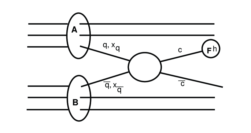
A shorthand method used to describe what is shown in Figure 1.1 is:

$$A+B\rightarrow D^{+}+D^{-}+X$$

where the charm quark hadronized into a $D^{+}$, the anti-charm quark hadronized into a $D^{-}\;$and $X$ is used to denote ’anything else’, which must include two baryons.

All mesons are unstable and decay. The short hand notation for one of the ways a $D^{+}\;$meson may decay, called a hadronic mode, is:

$$D^{+}\rightarrow K^{-}\;\pi^{+}\;\pi^{+}$$

An example of a decay mode referred to as a semi-leptonic mode is

$$D^{+}\rightarrow\mu^{+}\;\nu_{\mu}\,K^{-}$$

Experiments studying the production of open charm usually ’tag’ events by looking for the decay products from various decay modes. For the hadronic mode above, the event would be tagged if a $K^{-}\;$and 2 $\pi^{+}\;$tracked back to a common vertex, suggesting they were the decay products from the $D^{+}$. The invariant mass is then calculated, and compared to the mass of the $D^{+}$. If the event passes all cuts used to eliminate bad events, it is used in the analysis of the production characteristics of the $D^{+}\;$for their experiment.

This analysis used data from 800 GeV/c p-Cu  and p-Be  interactions to determine the production of hadrons containing open charm as a function of the hadron $p_{T}$. The data consisted of single muon events. The E866 spectrometer was designed to study di-muon events, where the two muons tracked back to a decay vertex. Single muon events are events where a hadron decays semi-leptonically to one muon, plus anything else, as shown above. The E866 spectrometer could not track any remaining secondary particles from the decay, so no decay vertex was available. The single muon data was taken from two production regions simultaneously, one a thin target of either copper or beryllium, the other a solid copper beam dump. The targets had an open decay length of 92 inches before hadrons (and remaining proton beam) interacted in the dump. Hadrons containing open charm decay roughly $10^{4}$ times sooner than light hadrons, so the ratio of muons from open charm to light hadrons is significantly enhanced in the data taken from the dump, relative to the data taken from the targets. Use of the difference between muon spectra from the two production regions allowed extraction of the inclusive open charm/anti-charm differential cross sections as a function of the hadron transverse momentum between 2.25 and 10.0 GeV/c. Mesons containing open charm are shown in Table 1.2.

Table 1.2: Mesons containing open charm. Mass (MeV/c²) is rounded off to the nearest MeV/c².

Pseudoscalar Mesons (Spin 0)
	$D^{+}$	$D^{0}$	$D^{+}_{s}$	$D^{-}$	$\overline{D}^{0}$	$D^{-}_{s}$
Quarks	$c,\overline{d}$	$c,\overline{u}$	$c,\overline{s}$	$\overline{c},d$	$\overline{c},u$	$\overline{c},s$
Mass	1869	1865	1969	1869	1865	1969
Vector Mesons (Spin 1)
	$D^{*\,+}$	$D^{*\,0}$	$D^{*\,-}$	$\overline{D}^{*\,0}$
Quarks	$c,\overline{d}$	$c,\overline{u}$	$\overline{c},d$	$\overline{c},u$
Mass	2010	2007	2010	2007

The term inclusive (versus exclusive) is used to classify the production of open charm by the final state of the reaction

$$p+N\rightarrow D+X$$

where $p$ is a proton interacting with a nucleon $N$ in the material, $D$ is a hadron containing open charm or open anti-charm and $X$ is anything else. This analysis could not identify the parent hadron, so any hadron produced that decayed to an open charm or anti-charm hadron is included in the measured cross sections as if it were produced as an open charm or anti-charm hadron, such as

$$p+N\rightarrow B+X\quad\mbox{where}\quad B\rightarrow D+\pi$$

Exclusive cross sections measure the strength of a reaction to a specific set of particles such as:

$$p+N\rightarrow\pi^{+}+\pi^{-}+p+N$$

Additional information can be derived as well, such as the production dependency on $A$. Prior experimental results from meson interactions have shown an enhancement of the production of open charm hadrons containing one of the valence quarks of the incident meson, called the leading particle effect. This enhancement has not been observed in proton interactions. If this effect were present in proton-nucleon interactions, it would be seen as an enhacement of hadrons relative to anti-hadrons. The hadron/anti-hadron ratio determined by this analysis is presented as well.

1.1 Heavy Hadron Production

The theoretical description of heavy hadron production in pQCD (perturbative Quantum Chromodynamics) is done in two parts, referred to as factorization; production of the heavy quarks using partonic cross sections, and the process of hadronization, where the bare quarks are transformed into hadrons seen in the lab.

A cross section, $\sigma$, is used to measure the effectiveness of an interaction such as

$$a+b\rightarrow c+d$$

where $a$ and $b$ are the interacting (incident) particles and $c$ and $d$ are particles produced in the interaction which may be different from either $a$ or $b$. The cross section has units of area, typically given as barns (1 barn = $10^{-24}$ cm²).

Partonic cross sections in QCD are modeled from Deep Inelastic Scattering cross sections. The cross sections for deep inelastic scattering on unpolarized nucleons can be written, generically, in terms of structure functions:

$$\frac{d^{2}\sigma^{i}}{dx\,dy}={\displaystyle\frac{4\pi\alpha^{2}}{xyQ^{2}}}\,\eta^{i}\,\left[\left(1-y-{\displaystyle\frac{x^{2}y^{2}M^{2}c^{4}}{Q^{2}}}\right)F^{i}_{2}+y^{2}xF^{i}_{1}\mp\left(y-{\displaystyle\frac{y^{2}}{2}}\right)xF^{i}_{3}\right]$$ (1.1)

where $i=NC,CC$ is for neutral or charged current scattering and $F^{i}_{1}$, $F^{i}_{2}$ and $F^{i}_{3}$ are structure functions. $Q$ is the four-momentum transferred in the interaction, and $\alpha$ (called the fine structure constant) is defined as $\alpha=e/\hbar c$. (The units for $\alpha^{2}$ are (GeV²   cm²).) In the quark-parton model, contributions to the structure functions are expressed in terms of quark distribution functions of the proton. The quark distribution function, $q(x,Q^{2})$, is the number of quarks, or anti-quarks, of the designated flavor ($q=u,\overline{u},d,\overline{d},s,\cdots$) that carry a momentum fraction between $x$ and $x+dx$ of the protons momentum where the protons momentum is large. For the charged current reaction $e^{-}p\rightarrow\nu X$

$$F^{W^{-}}_{2}=2x\left(u+\overline{d}+\overline{s}+c+\cdots\right)$$

One prediction of the quark-parton model is that the structure functions scale in the Bjorken limit that $Q^{2}$ and $\nu\rightarrow\infty$ with $x$ fixed. Scaling implies

$$F^{i}(x,Q^{2})\rightarrow F^{i}(x)$$

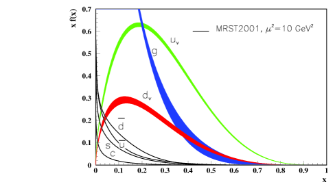
QCD uses scale dependent parton distribution functions (PDFs), $f(x,\mu^{2})$, to describe the process above. Here, $f=g\,\mbox{or}\,q$ and $\mu$ is typically the scale of the probe, $Q$. At a given $x$, these correspond to the density of the partons in the proton integrated over transverse momentum $k_{t}$ up to $\mu/c$. The fine structure constant $\alpha$ used in Equation 1.1 is redefined to be scale dependent $\alpha_{s}(\mu^{2})=\frac{g^{2}_{s}(\mu^{2})}{\hbar c}$ where $g_{s}$ is the SU_c(3) coupling constant. Parton distributions have been measured by many experiments. Figure 1.2 shows the distributions $x$ times the unpolarized parton distribution functions $f(x)$ at a scale $\mu^{2}=10$ GeV²/c^-2.

Figure 1.2: Distributions of $x$ times the unpolarized parton distributions $f(x)$ (where $f=u_{v},d_{v},\overline{u},\overline{d},s,c,g$) using the MRST2001 parameterizations [2, 3] (with uncertainties in $u_{v},d_{v}$ and $g$) at a scale $\mu^{2}=10$ (GeV²/c²). Figure is taken from [1].

Production of heavy quarks in hadron-hadron interactions at leading order (LO) in perturbation theory is the result of two parton-parton interactions

$$q\,\overline{q}\rightarrow Q\,\overline{Q}\quad\mbox{and}\quad g\,g\rightarrow Q\,\overline{Q}$$

where $q\,\overline{q}\,$ (often referred to as quark-quark annihilation) represents a quark from one hadron interacting with an anti-quark from the other hadron, $g\,g$ is used to represent the interaction between a gluon in one hadron interacting with a gluon in the other, and $Q\,\overline{Q}\,$ is the produced heavy quark and anti-quark (they must be produced as a pair). In p-p  or p-A  collisions, $q\,\overline{q}\,$ interactions are between a valence quark in one hadron, and a sea anti-quark in the other.

Feynman diagrams are used to describe the process as well as to calculate the amplitudes of the interaction. The Feynman diagrams of the leading order (LO) processes for the production of charm are shown in Figure 1.3. The total partonic cross section from hadro-production is proportional to the sum of all the combinations of the quarks in one hadron with anti-quarks in the other (and conversely, the sea anti-quarks in the first with quarks in the other) plus the contribution from gluons in both.

Figure 1.3: The Leading Order Feynman diagrams $q\,\overline{q}\rightarrow Q\,\overline{Q}$ (1) and $g\,g\rightarrow Q\,\overline{Q}$ (2).

Hadronization is usually described in terms of fragmentation functions, $F(x,s)$. The Particle Data Group [1] define the fragmentation function for a hadron of type $h$ at c.m. energy $\sqrt{s}$ represented as a sum of contributions from the different parton types $i=u,d,s,\overline{u},\overline{d},\overline{s},\cdots,g$ as

$$F^{h}(x,s)=\sum_{i}\int^{1}_{x}\frac{dz}{z}\,C_{i}(s;z,\alpha_{s})\,D^{h}_{i}(x/z,s)$$ (1.2)

where $D^{h}_{i}$ are the parton fragmentation functions analogous to the parton distribution functions above, $x=2\,E_{h}/s\leq 1$, $z=x_{h}/x_{i}$ and $C_{i}$ are coefficient functions of the partons $i$.

At lowest order in $\alpha_{s}$, the coefficient function $C_{g}$ for gluons is 0, but for quarks, $C_{i}=g_{i}(s)\,\delta\left(1-z\right)$. At higher orders of $\alpha_{s}$ the coefficient and parton fragmentation functions are factorization scheme dependent. Measured fragmentation functions need to be parameterized at some initial scale, $t_{0}$, typically 2 GeV² for light quarks and gluons. A general parameterization is:

$$D_{p\rightarrow h}=N\,x^{\alpha}\,\left(1-x\right)^{\beta}\,\left(1+{\displaystyle\frac{\gamma}{x}}\right)$$

where the normalization $N$, $\alpha$, $\beta$ and $\gamma$ are usually dependent on the scale $t_{0}$ as well as the type of parton, $p$ and hadron $h$.

There have been numerous studies of the production of open charm using nuclear targets. The majority of fixed target studies have been done using charged meson beams on nuclear targets. A reasonably complete compilation of experimental results is found in [5]. Here, and in most literature, the term open charm production is used as a ’catch all’ phrase for all hadrons containing one charm or anti-charm quark. Results are usually presented for the total open charm production, or one or more sub-categories of these hadrons, such as hadrons containing one charm quark ($D$) or one anti-charm quark ($\overline{D}$) or those with charge $\pm$1 or neutral.

1.2 Results From Prior Experiments

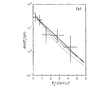
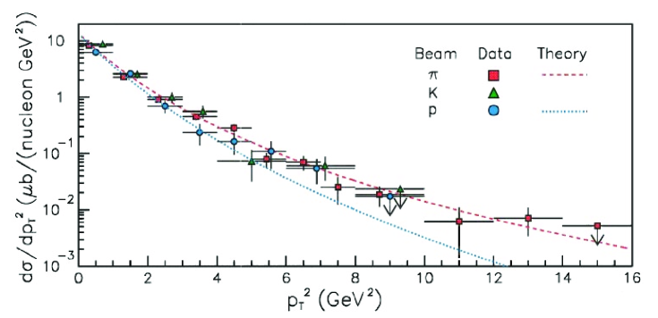
Discussion concerning results from fixed target p-p  and p-A  open charm production often cite publications from four experiments; Fermilab Experiment 743 (the LEBC-MPS Collaboration) [6], Fermilab Experiment 653 [7], Fermilab Experiment 789 [8] and Fermilab Experiment 769 [9, 10]. Figure 1.4 shows the total open charm differential cross section from 800 GeV/c p-p  interactions as measured by the LEBC-MPS Collaboration [6].

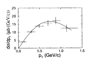
Fermilab Experiment 789 measured neutral open charm production for 800 GeV/c protons incident on beryllium and gold targets [8]. Their results are shown in Figure 1.5. The Fermilab E769 Collaboration studied open charm production using secondary 250 GeV/c $\pi^{\pm}$, $K^{\pm}$ and $p$ beams on a multifoil target of beryllium, copper, aluminum and tungsten [9, 10]. The results from [9] are presented in Figure 1.6.

The production of open charm using charged meson beams shows significant differences from the production of open charm using proton beams on nuclear targets. The differences are seen in the ratio of charged to neutral charm production and the ratio of hadron to anti-hadron production. The second is referred to as the leading particle effect. Results to date from either meson or proton induced production reveal that open charm meson production is shaped more or less the same as the next-to-leading order (NLO) predictions for the production of the quarks themselves (see Figure 1.6).

Theory suggests that the ratio of charged to neutral open charm production should be approximately 0.32 [5, 12], and results from open charm production using charged meson beams shows rough agreement. The results from fixed target p-p  and p-A  experiments, until recently, have shown this ratio to be more or less unity. A recent result published by the HERA-B Collaboration reports the ratio $\sigma(D^{+})\,/\,\sigma(D^{0})=0.54\pm 0.11\pm 0.13$ from 920 GeV/c p-A  induced production [13]. The STAR Collaboration reported the same ratio as 0.40 $\pm$ 0.09 $\pm$ 0.13 using data from $\sqrt{s_{NN}}=200$ GeV p-p  and d-Au collisions [14]. The leading particle effect reported by meson-nucleon experiments is contrary to predictions as well. Proton-nucleon experiments have not seen this effect. It is generally thought that some momentum is lost during the hadronization process. Results from a variety of experiments, such as E769 above, do not show this effect.

Figure 1.4: Total inclusive open charm differential cross section $d\sigma(D+\overline{D})\,/\,dp^{2}_{T}\,$ ($\mu$b c² GeV^-2) measured by the LEBMC-MPS Collaboration (Fermilab Experiment 743)[6]. Solid curve shows the results of a fit to the empirical form $\left(1-|x_{F}|\right)^{n}\,exp\left(-a\,p_{T}^{2}\right)$.

Figure 1.5: Differential cross section per nucleon, $d\sigma(D^{0})\,/\,d\,p_{T}+d\sigma(\overline{D}^{0})\,/\,d\,p_{T}$ versus $p_{T}$. Uncertainties shown are statistical only and do not inclue an additional systematic uncertainty of 12.8 percent. Figure is from Fermilab Experiment 789[8].

Figure 1.6: Measured $D$ meson $(D^{+},\,D^{-},\,D^{0},\,\overline{D}^{0},\,D^{+}_{s}\,\mbox{and}\,D^{-}_{s})\quad d\sigma\,/\,dp^{2}_{T}\,$ $\left(\mu\mbox{b}\,\mbox{c}^{2}\,\mbox{nucleon}^{-1}\,\mbox{GeV}^{-2}\right)\,$ $\left(x_{F}>0\right)\,$ for production induced by $\pi$, $K$ and $p$ beams and NLO QCD predictions for charm quarks [11] ($\pi$ and $p$ beams). In addition to the statistical errors shown, there are overall normalization errors of about 6%, 6% and 9% for $\pi$, $K$ and $p$ results respectively. Figure is taken from [9].

Chapter 2 Apparatus

2.1 General Description

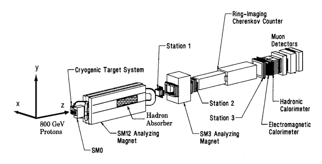
Fermilab Experiment 866 (E866/NuSeA) was designed for collecting and analyzing di-muon events from 800 GeV/c protons incident on various nuclear targets. E866 was a continuation of several Fermilab Experiments including 772 and 789, where the detector had several major improvements to increase the accuracy of the measured trajectory of the muons as well as increased data taking capabilities through improvements in the data aquisition system and trigger configurations. The experiment has resulted in five previous Doctoral theses [16] - [20] and several published results [21]$\,-\,$[27].

Figure 2.1 shows the FNAL E866/NuSeA spectrometer for the original configuration of the experiment. There were modifications to the original configuration to take data for this analysis that will be pointed out and explained as necessary.

The E866 spectrometer was located in the East hall of the Meson Experimental Area, and used the 800 GeV/c proton beam extracted from the accelerator ring for a period of approximately twenty seconds out of each minute. Each spill contained ”buckets” with a 19 $ns$ time structure based on the radio accelerator RF of 53 MHz.

Figure 2.1: FNAL E866/NuSeA Spectrometer. For this analysis the spectrometer had no cryogenic target system, but a target wheel instead, missing is the dump shown in figure 2.2. The ring-imaging cherenkov counter was inactive, and the muon detectors are referred to as station 4 in the text.

2.2 Beam Monitors

Beam monitoring was accomplished with various detectors for size, position and intensity. The beam size and position was measured using RF cavities and segmented wire ion chambers (SWIC). The beam was last monitored approximately 70 inches upstream of the targets. This was done using a movable SWIC having a wire spacing of 2 mm horizontally and 0.5 mm vertically. There were several intensity monitors, but these were unreliable at the low intensity (approximately $10^{10}$ protons per spill) used for the single muon data.

2.3 Targets

The data was taken with a rotating target wheel instead of the cryogenic target system shown in Figure 2.1. The experiment designated the center of the opening of the upstream face of spectrometer magnet SM12 as the origin. The target wheel was located at $z=-24$ inches. The wheel had three used positions; one empty target frame, one beryllium target of thickness 2.036 inches (referred to as the beryllium target), and another copper target of thickness 1.004 inches (referred to as the copper target). The proton interaction lengths of these targets, calculated with $\rho_{Cu}=8.96$ gm cm${}^{-3}\;$and $\lambda_{I,Cu}=134.9$ gm cm${}^{-2}\;$for copper and $\rho_{Be}=1.848$ gm cm${}^{-3}\;$and $\lambda_{I,Be}=75.2$ gm cm${}^{-2}\;$for beryllium, were 0.127 and 0.169 interaction lengths respectively. The wheel was rotated during the 40 second period between spills according to two rotation schedules.

2.4 Spectrometer

The spectrometer had three dipole magnets with fields in the $x$ direction as defined in Figure 2.1. For this analysis data was taken with currents in magnets SM12 and SM3 only. The currents were configured both parallel and anti-parallel during data taking, although results are only shown for the parallel configuration. The magnet currents were set to 1420 amps in SM12 and 4200 amps in SM3. Only the results from the parallel magnetic field configuration are given in this analysis, because the analysis lost the computer during the analysis of the opposite polarity data. The magnetic configuration would only allow for a separate set of data to fit, since combining the two results was not possible. The acceptances for both magnetic field configurations was very similar, so no new information was lost.

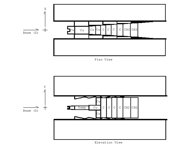
Particles created in the targets, and any remaining proton beam, entered magnet SM12. The configuration of this magnet when the data for this analysis was taken is shown in detail in Figure 2.2. The magnet was 567 inches long and provided a momentum deflection of 7 GeV/c when operated at its maximum current of 4000 amps and provided a momentum deflection of approximately 2.4 GeV/c for this data. The copper beam dump was 168 inches long beginning 68 inches inside the volume of the magnet. The dump spanned the entire volume in $x$, and was approximately 8 inches tall for the first 80 inches, and 10 inches tall thereafter. The face of the dump had a rectangular hole 12 inches deep by 2 inches square to reduce back-scattered particles. The dump provided a second target having 26 proton interaction lengths, or approximately 220 radiation lengths.

Behind the dump was the hadron absorber that filled the entire volume in $x$ and $y$ consisting of 24 inches of copper, 4 layers of carbon 27 inches thick each and two 36 inch layers of borated polyethylene. The absorber wall, having over thirteen interaction or sixty radiation lengths, effectively allowed only muons to pass downstream. The remainder of the inside of the magnet was filled with a helium bag.

Figure 2.2: Spectrometer magnet SM12 as configured for this analysis showing the copper beam dump and hadron absorbers in plan view (top) and elevated view (bottom). Cross indicates the location of the targets relative to the spectrometer magnet and dump.

Between magnets SM12 and SM3 is the first of three similar tracking stations. Stations 1, 2 and 3 had multiple pairs of drift chambers and one or more layers of hodoscopes. Station 1 had three pairs of drift chambers, U1, U1^′, Y1, Y1^′ and V1 and V1^′. Planes U and U^′ had sense wires oriented +14^∘ $\left[tan(\theta)=0.25\right]$ in the $x-y$ plane, Y and Y^′ were horizontal and V and V^′ were oriented -14^∘. The primed planes were offset in the direction perpendicular to the sense wires by half of one cell to help remove ambiguities in the drift direction. Table A.1 (page A.1) gives a summary of the physical characteristics of the drift chambers for each station.

Hodoscopes at each station allowed fast track evaluations or ’roads’ used to trigger valid events to be taken to tape. Horizontally aligned planes of scintillators determined rough $y$ positions, while vertically aligned planes gave rough $x$ positions. Each plane was optically split to provide quadrants named up left (UL), up right (UR), down left (DL) and down right (DR). Each plane was designated by orientation and station number. Gaps created in the splitting resulted in small dead spots for muon tracks at or near $x=0$ for $y$ hodoscope planes, or $y=0$ for $x$ hodoscope planes.

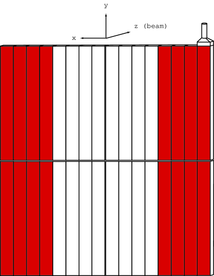
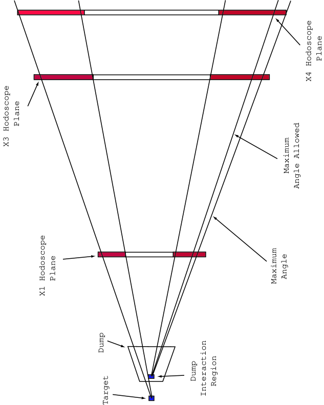
Specific to this analysis, data were taken with the middle half of each $x$ measuring hodoscope plane turned off to reduce trigger rates that would have been unacceptabes had they been left on. This configuration was necessary to reduce the event rate, even at the low intensity requested. This configuration produced a loss in acceptance for muons having $p_{T}\left(\mu\right)\leq 1.75GeV/c$, and created two inner acceptance edges which further reduced the acceptable minimum muon transverse momentum as described in 2.5 and 3.3. Figure 2.3 shows an $x$ hodoscope plane, and Table A.2 gives the specifications of all hodoscope planes as used for taking data for this analysis.

Figure 2.3: View of an $x$ plane of hodoscopes. Gaps between quadrants are exaggerated. Only one phototube is shown. Shaded region represents hodoscopes having high voltage supplied to the attached phototubes. $y$ hodoscopes are similar except being rotated 90 degrees and all scintillators have high voltage supplied to the phototubes.

Particles then entered the second magnet, SM3, which was used to determine the momentum of the particle in the $y-z$ plane. At its normal current setting of 4230 Amps, the magnet provided a transverse momentum deflection of 0.91 GeV/c. The direction of the deflection relative to the magnetic field direction determined the charge of the particle. Muons then passed Station 2, a tracking station similar to Station 1 except only one plane of $y$ measuring hodoscopes, Y2, is present.

Muons then traversed a non-operational Ring Imaging Cherenkov counter (RICH). This detector had been used in previous experiments for particle identification, but was not used for this analysis. The interior was helium filled to reduce multiple scattering. Downstream of the RICH detector was Station 3, a larger version of the prior stations. Station 3 had both $x$ and $y$ measuring hodoscope planes.

Both calorimeters following Station 3 shown in Figure 2.1 were inactive, but had been left in place to provide additional hadron absorbing material. Shown in Figure 2.1 are large amounts of zinc and concrete placed between three layers of proportional tubes, PTY1, PTY2 and PTX in Station 4, labeled as ’Muon Detectors’ in figure 2.1. Station 4 had two hodoscope layers for measuring both $x$ and $y$, called Y4 and X4.

All wire planes and proportional tubes used the same gas mixture, 50% argon, 50% ethane and a small amount of ethanol alcohol added by bubbling the gas through ethanol which was kept at a constant 25^∘ $F$.

2.5 Special X Hodoscope Setting

The single muon analysis used a special configuration of the $x$ measuring hodoscopes. The high voltage supply for the middle half of all $x$ hodoscope layers was turned off (referred to as being pulled), shown in figure 2.3. This reduced the event rate for single muon events as well as providing a way to distinguish between events from the target and dump. This was a significant change from the normal operation of the apparatus. Single muon events required hits on the same side in all three $x$ hodoscope layers. This $x$ hodoscope configuration plus the required trigger, described in 2.6, limited the transverse momentum of accepted events, because the muon must have a minimum absolute value for the slope in the $x-z$ plane, $|\mbox{TAN}\theta_{x}|=|\overrightarrow{p}_{x}/\overrightarrow{p}_{z}|$. This minimum slope is shown in figure 2.4. The figure also shows how the loss in acceptance allowed separation of target and dump events for single muons. The minimum and maximum $|\mbox{TAN}\theta_{x}|$ for muons to be accepted, based on the spectrometer survey are listed in Table A.2.

Figure 2.4: Drawing of change in acceptance of the spectrometer in the $x-z$ plane, as well as the minimum and maximum opening angles caused by disconnecting the high voltage supplies to the middle half of the hodoscopes in all $x$ hodoscope planes. Note the extreme shortening of the $z$ axis, though relative distance from targets to hodoscope planes is preserved. Maximum angle refers to the maximum physical opening, while maximum angle allowed is the angle in the final cuts to insure all events passed through a hodoscope in all three planes.

2.6 Event Triggers and Readout

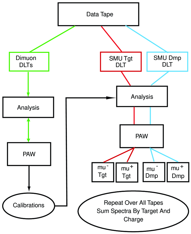
The FNAL E866/NuSeA trigger has been described in detail in several references [28] [29]. The data taken for the single muon analysis contained both single and dimuon events, requiring dimuon as well as single muon triggers. Dimuon events were used to calibrate the analysis routine as described in Chapter 3. The calibrations found from the di-muon events were then used to analyze the single muon events.

Signals from the hodoscopes were first sent to LeCroy 4416 discriminators whose signals were reshaped and synchronized to the accelerator RF clock. All triggers are hit correlations from some or all hodoscope layers and are referred to as Physics A, Physics B and Diagnostics triggers. The single muon data was taken using 5 single and 5 dimuon physics triggers in two separate but similar configurations. The trigger system for the left half of the spectrometer is shown in figure A.1 [16].

The trigger system had a total propagation delay from inputs from hit hodoscopes to output of the event to memory storage of approximately 20 nsec, providing single bucket resolution. This was accomplished by comparing hodoscope hits in the seven layers to hardwired and software defined matrices in modules called Track Correlators (TCs) or Matrix Modules (MMs). The four Trigger Matrix modules (called MUL, MUR, MDL and MDR) were lookup tables loaded onto a set of ECL SRAM chips. These modules used correlations in the Y1, Y2 and Y4 hodoscopes only. A track of interest would define a ’road’ in the Y view under the deflection of the magnetic fields in SM12 and SM3. Hits on Y2 and Y4 were correlated against predicted hits on Y1 and if the desired correlation existed, output for the event was generated. These were used only for dimuon events. Four S4XY Track Correlators, also used for di-muon events only, used signals from the X4 and Y4 hodoscopes only. The correlations required for a di-muon event to be accepted could be changed by software.

The three $x$ hodoscope layers were hardwired into an and for each side, called X134L and X134R. Any muon which traversed an energized hodoscope paddle in all three $x$ layers on one side satisfied the X134 trigger.

These were passed to the two main physics Track Correlators (along with the other information from the Matrix Modules and S4XY Track Correlators) called Physics Triggers TC and Diagnostic Triggers TC. These two main correlators determined the validity of an event and if it was to be taken to tape, then informed the Master Trigger to set the busy signal and stream the event to a large memory buffer, and subsequently written to 8mm tape.

The di-muon triggers were labeled Physics TcA1 through 4, Diagnostic 3 and all four S4XY triggers. All dimuon triggers were not prescaled due to the low beam intensity.

One example of an opposite sign dimuon pair physics trigger was a coincidence of a track through the upper and lower left (or alternatively right) quadrants (one being the $\mu^{+}\;$and the other the $\mu^{-}$), and an example for a like sign dimuon event where one muon goes through the upper right quadrant in coincidence with a muon passing through the upper left quadrant, all using the four Matrix Modules MUL, MUR, MDL and MDR. The Diagnostics trigger required a left-right coincidence in five of the seven layers of hodoscopes on both sides of the spectrometer.

The X134L/R three-fold coincidence trigger, called PhysB1, was the exclusive single muon trigger used for analysis. For diagnostics purposes there were 4 other single muon triggers, PhysB2, Diag1, Diag2 and Diag4. The diagnostic triggers were useful for studying edge effects of the pulled hodoscopes as well as hodoscope efficiencies for two of the three X layers.

The first trigger, PhysB1, required a hit in all three X hodoscope banks on either side. PhysB2 was a prescaled trigger to take 1 of 2000 events where there was a track through a quadrant (any one quadrant of the four) using the MUR/L MDR/L matrix modules, thus avoiding the large opening angle required for trigger PhysB1.

The main single muon event trigger was PhysB1, called the X134L/R trigger referring to the three fold coincidence of the three X hodoscope planes on either side, left or right. This trigger is often referred to by the single muon analysis as the ’trigger bit 5’ trigger since that bit was set if the event had that coincidence. All single muon events were required to have a valid PhysB1 trigger set.

All events satisfying one or more triggers were written to tape. This was accomplished using Nevis Transport electronics [29], and VME as well as CAMAC modules. All detector subsystems fed data onto the Transport bus, which was then transferred to the memory buffer. The memory buffer, which was VME based, formatted the event data and transferred it to 8mm tape. Since the typical spill lasted 20 seconds out of every minute, the memory buffering allowed higher event rates with less deadtime. Each event written to tape contained the values from the coincidence registers from the hodoscopes and proportional tubes and readouts from the time to digital converters (TDC’s) from signals in the drift chambers, as well as beam position, size and intensity, target position, voltages and information from various monitors.

2.7 The Single Muon Data

Table 2.1: Data taken for this analysis. All data were taken with a common trigger configuration. Currents in SM12 and SM3 set to -1400 and -4200 amps, respectively. All data was taken using the same trigger configuration file, labeled jpsism2. The triggers for this configuration are given in the text.

			Events
Run	Date	Time	$\times\,10^{6}$	Trigger
2748	07/10/97	10:14	5.778	jpsism2
2749	07/10/97	14:06	6.047	”
2750	07/10/97	15:41	6.067	”
2751	07/10/97	17:16	5.918	”
2752	07/10/97	19:40	5.942	”
2753	07/10/97	21:42	5.750	”
2754	07/10/97	23:30	7.995	”
2755	07/11/97	01:38	6.172	”
2756	07/11/97	03:41	5.944	”
2757	07/11/97	06:06	3.150	”

Chapter 3 Analysis

The 10 runs on 10 tapes listed in Table 2.1 (page 2.1) contained the single muon data used in this analysis. The E866 collaboration analyzed data for dimuon events with an analysis routine first developed for the E605 experiment. The dimuon code was modified to analyze both single and dimuon events for this analysis. All modifications to the original routines are presented in detail. Analysis of the single muon data was performed in four stages;

1. Separate single from dimuon events, separate target events from the dump events, then place the separated raw data into Data Summary Tapes, or DSTs, for further analysis.

2. Iterative analyses of the dimuon DSTs were then performed to determine the correct values, or calibrations, needed to initialize the code. No further analysis of dimuon data was performed.

3. Multiple analyses of the single muon data was performed using the single muon DSTs, placing the fully analyzed events into large arrays called n-tuples.

4. Output final data (the single muon spectra) to arrays for use in the fitting routines to determine the open charm cross sections.

Figure 3.1 shows a flow chart of the method used to analyze the single muon data, and may be useful for the following discussions. All analysis of the raw data as well as generation and analysis of Monte Carlo events was performed on a DEC Alpha 500 workstation.

Figure 3.1: Flow chart of the process used to analyze the single muon data. The data was histogrammed as a function of the muon $p_{T}\;$and placed into arrays for use in the least-squares minimization routines described in Chapter 5. Each target resulted in four spectra, one each for $\mu^{+}\;$and $\mu^{-}\;$from the target and one each from the dump.

3.1 Initialization and Unpacking

The first step in the analysis code was to initialize for the specific run. This initialization included setting the magnetic fields in SM12 and SM3 to the current direction and value at the start of the run, trigger information and input spectrometer calibrations. The code identified the number of the run from the data tape and used an internal look up table to set the magnetic field configurations whereas the trigger information and spectrometer calibrations needed were read from specified trigger or data tables.

The code then unpacked and processed the events. Unpacking an event was a process that read the output DAQ information contained on the tape for that event and allocated the information to several large arrays which were designed to speed up the analysis of each track.

3.2 Tracking

Tracking began with searching for hit clusters in all the wire planes in Stations 2 and 3 (See Figure 2.1, page 2.1). This required hits in 4 of the 6 planes in each station to qualify as a potential hit cluster. Those clusters having hits in 2 of the 3 planes were classified as doublets, those having all three planes registering a hit were classified as triplets. All clusters required at least one hit in the Y view plane. Once a list of doublets and triplets had been made, combinations of hits in the two stations were linked to produce track candidates. The linkage was a combination of hit clusters that loosely pointed back to the target region.

The next tracking process was to extend the candidate tracks to hit clusters in the Station 1 chambers. Each candidate track was projected upstream through SM3 in the x-z plane to a vertical band in Station 1. Only clusters found within this band were considered for that track. If a cluster was found in the band, the entire track from Station 1 to Station 3 was refit using all 18 wire planes in the three stations. The $z$ coordinate in SM3, $Z_{SM3}$ was allowed to vary. All tracks required at least 14 hits in the 18 planes. The final fit at this point in the tracking routine gave the position of the track in $x$, $y$ and $z$ (called $X_{SM3}$, $Y_{SM3}$ and $Z_{SM3}$ respectively) at the SM3 bend plane as well as the slopes $\mbox{TAN}\theta_{x}$(SM3) and $\mbox{TAN}\theta_{y}$(SM3), where $\mbox{TAN}\theta_{x}\,$and $\mbox{TAN}\theta_{y}\,$are the ratios of the $x$ and $y$ momenta to the $z$ momentum using the sign convention that $\mbox{TAN}\theta_{x}\,$(or $\mbox{TAN}\theta_{y}\,$) is positive if $\overrightarrow{p}_{x}\;$or $\overrightarrow{p}_{y}\;$is in the positive $\hat{x}\,\mbox{or}\,\hat{y}$ direction.

The difference $\mbox{$\mbox{TAN}\theta_{y}$}^{U}(SM3)-\mbox{$\mbox{TAN}\theta_{y}\,$}^{D}(SM3)$, where U and D refer to upstream or downstream of the SM3 bend plane, with the field map of SM3 determined the y-z projection of the momentum. Combined with $\mbox{TAN}\theta_{x}$(SM3), the four momentum $\left(\frac{E}{c},\,\overrightarrow{p}\right)$ at Station 1 was fully determined. A final cut on the 18 plane fit requiring the track to have $\chi^{2}_{pdf}\;$less than 5 was made.

The full reconstruction of the track downstream of Station 1 was then completed. Each track found above making all cuts was projected back to Station 4. Since there was considerable hadron absorber material throughout this projection, the projected intercept at Station 4 was compared to a ’window’ of possible hits in the 3 proportional tube layers as well as the hodoscopes. These windows were wide enough to allow for multiple scattering within 5 standard deviations at each detector plane around the projected straight line intercept. High momentum tracks had windows of less than a few cells. The detectors were then scanned for hits within the windows. A track was further considered if it had 3 of the 5 planes (3 proportional tube planes and 2 hodoscope planes) registering a hit.

This procedure was done for all candidate tracks found from the event on tape, and the resulting number of such tracks as well as numbers of hits, clusters and fitting information was passed to arrays for further use.

3.3 Trace-back Through SM12

Once all candidate tracks for an event were found, the event was passed to a section of code that would ’trace-back’ each candidate track to the assumed place of origin on the $z$ axis, $Z_{tgt}$. For this Chapter, ’target’ (such as $tgt$ in $Z_{tgt}$) is used to denote either the actual targets in the target wheel (target analysis), or the dump (dump analysis), unless it is necessary to distinguish between the two. This was done sequentially to each track in the order they were found in the tracking section of the code. Since there were no detectors upstream of Station 1, this was done using the magnetic field map of magnet SM12 as well as experimentally determined energy losses for the absorber materials [30], to ’project’ the most probable path of the muon back toward its assumed origination. Once this projection was calculated, the effects of multiple scattering were added by use of a single bend plane approximation, resulting in the final calculated momenta for the muon at its assumed point of origin.

The trace-back section of the analysis code is described here as it was originally written. The single muon analysis made several changes to the procedure which will be described in Section 3.5.1, however, the basic trace-back was preserved and valid for either dimuon or single muon events. Trace-back was done in three stages for each track found.

The first stage entailed adding back in lost energy due to interactions within materials as well as changes in trajectory due to the magnetic field within magnet SM12 beginning at $Z_{SM3}$, the location of the bend plane in SM3. The trace-back procedure ’swam’ the particle back to a fixed point along $z$, called $Z_{tgt}$, which was either the location of the thin targets ($z=-24.0$ inches) for target events, or a fixed $z$ location inside the dump for dump events ($Z_{tgt}$ for dump events was set to the distance at which 1/2 of the protons intering the dump would have interacted, $Z_{tgt}=85.1$ inches).

The code began by adding in the beam offsets $X_{off}$ and $Y_{off}$, and then trace the muon upstream until it reached either the beginning of the copper dump at $z=68$ inches for target events, or until the next incremental distance in $z$ (referred to as sections which were 2 inches in length) upstream of $Z_{tgt}$ where events from the dump were forced to originate from.

Candidate tracks must pass cuts requiring the track to actually remain within the volume of the magnet during the trace-back. The x-y plane at $Z_{tgt}$ was called the analysis plane. The placement of the forced points of origination are discussed in detail in Section 3.4.2.

Corrections for energy loss used the mean energy loss for a muon in 2 inches of the material being traversed [30]. The materials, in the order taken by the trace-back procedure, were 72 inches polyethylene, 108 inches carbon, 24 inches copper (called the copper wall) and either up to 168 inches of copper for target events or about 151 inches of copper for dump events. The amount of the copper dump traversed was stored for use during the second stage of the trace-back.

The second stage of the trace-back used the amount of dump material the track had traversed to determine the location along $z$ at which correction for multiple scattering should be done. The analysis code used a single bend-plane approximation to correct for multiple scattering that occured while the muon traversed the dump and hadron absorber materials in magnet SM12. The single bend-plane approximation was based on determining a point along the $z$ axis called $Z_{scat}$, where the effects of the multiple scattering could be approximated in a single large scatter, or bend (see for example [31]). The location of $Z_{scat}$ was calculated using

$$Z_{scat}=a\,l_{dmp}+min$$

where $a$ is a percentage of the amount of dump material traversed and $min$ is the minimum distance along $z$ at which the plane could be set. Since all single muon events required full traversal of the dump, which restricted all hadrons to have a set open decay length, $a$ was set to 0.

The multiple scattering correction required retracing the muon from downstream of magnet SM12 to $Z_{tgt}$ (at either the targets or in the dump), storing the 3 momenta $\overrightarrow{p}_{scat}$ and position $(X_{scat},Y_{scat},Z_{scat})$ found at $Z_{scat}$ during the trace-back, as well as the position $(X_{tgt},Y_{tgt},Z_{tgt})$ at $Z_{tgt}$. $X_{tgt}$ and $Y_{tgt}$ are commonly referred to as the uniterated $x$ and $y$ intercepts at the analysis plane. The difference between the uniterated intercepts and the beam centroids, $\Delta X$ and $\Delta Y$ , as well as an angular difference or correction to the track, $\Delta\theta_{x}$ and $\Delta\theta_{y}$ were calculated using

$$\left(\begin{array}[c]{l}\Delta X\\ \Delta Y\end{array}\right) =\left(\begin{array}[c]{l}X_{tgt}-X_{off}\\ Y_{tgt}-Y_{off}\end{array}\right)$$ (3.5)

$$\left(\begin{array}[c]{l}\Delta\theta_{x}\\ \Delta\theta_{y}\end{array}\right) =\frac{1}{Z_{tgt}-Z_{scat}}\left(\begin{array}[c]{l}\Delta X\\ \Delta Y\end{array}\right)$$ (3.10)

The third stage was an iterative process of tracing the muon back to the analysis plane from the scattering plane and testing the iterated $x$ and $y$ intercepts at the analysis plane against a distribution of acceptable values for $X_{tgt}$ and $Y_{tgt}$. If the current trace-back failed, new values for the angles $\Delta\theta_{x}$ and $\Delta\theta_{y}$ were calculated and the process was repeated. The kinematical variables (all referred to as iterated variables) were calculated after this final step in the retracing of the muon.

3.4 Spectrometer Calibrations

The analysis code required several input parameters to be set during initialization. The calibrations required were a scalar multiple for the magnetic field strength of SM12, called TWEE, the beam offsets $X_{off}$ and $Y_{off}$, used to center the beam at $Z_{tgt}$, the beam angles XSLP and YSLP and the position at which to place the scattering plane, $Z_{scat}$, called ZSCPLN.

Since the targets were relatively thin, it was assumed that the most accurate calibration for the magnetic field strength scalar, TWEE, would be found by fitting the dimuon data to the $J/\Psi$ mass (3.097 GeV c^-2). The calibrations for dump analyses were then found using this field scaler, with a small variation (less than 2 percent) allowed for uncertainties in the field map as well as the effect of the thickness of the target and location of the plane of analysis used for dump events. All dimuon target analyses used data taken with the beam incident to all three targets while analyses for determining the dump calibrations only used data taken with the target wheel at the empty position.

The calibrations were determined using an iterative process, changing the value for one of the variables and performing a new analysis of the Data Summary Tape. Results were plotted and subsequent changes were made to optimize the variable for that run. After all variables were determined for both target and dump the code was calibrated with the final settings and the initial reductions for single muons from that run were performed. Calibrations for this analysis are given in Table B.2 page B.2.

3.4.1 Cuts Used For Dimuon Events

The cuts on dimuon events used for determining the optimal spectrometer calibrations were:

1. Valid PhysA1, 2, 3 or 4 trigger must be set.

2. Event must have only two candidate tracks.

3. Event must have two valid tracks after tracing section of code.

4. Event must have oppositely charged muons. (Opposite sign pair.)

5. The estimated $z$ vertex, ZUNIN, must be within 50 inches of $Z_{tgt}$.

6. $\mbox{$\mbox{TAN}\theta_{y}\,$}\leq 0.030$ for both $\mu^{+}\;$and $\mu^{-}$.

7. $\mbox{$\mbox{TAN}\theta_{x}\,$}\leq 0.028$ for both $\mu^{+}\;$and $\mu^{-}$.

8. $2.1<m_{\mu\mu}<4.1$ (GeV c^-2).

The cut on $\mbox{TAN}\theta_{y}\,$was to insure both muons from the event traversed the entire length of the dump as explained in Section 3.5.2. The cut on $\mbox{TAN}\theta_{x}\,$was used to reduce the number of events where either muon may have scattered back into the acceptance after interacting in the walls of SM12, and $m_{\mu\mu}$ is the reconstructed mass of the dimuon pair in GeV c^-2.

To select higher quality events, the E866 analysis code calculated an estimate of the position along the $z$ axis where the parent hadron would have been created for the dimuon pair being analyzed. This calculation was based on information found as the two muons were traced back to the analysis plane at $Z_{tgt}$ during the second stage of the trace-back. The second trace-back section of code determined the four intercepts, $X_{tgt}^{\pm}$, and $Y_{tgt}^{\pm}$ as well as the two four momenta, $(\frac{E^{\pm}}{c},\overrightarrow{p}^{\pm})$ at $Z_{tgt}$ where $\pm$ refers to the two muons, $\mu^{+}\;$and $\mu^{-}$, of the dimuon pair. The distance in $y$ between the pair was calculated by $Y_{tgt}^{-}-Y_{tgt}^{+}$, and the estimated $z$ vertex of the parent hadron, ZUNIN, was then calculated using:

$$ZUNIN=-\left[\frac{Y_{tgt}^{-}-Y_{tgt}^{+}}{(\mbox{$\mbox{TAN}\theta_{y}$}^{-}-\mbox{$\mbox{TAN}\theta_{y}$}^{+})}\right]\quad\mbox{(inches)}$$ (3.11)

The smaller the absolute value of ZUNIN calculated, the more likely the parent hadron was produced at or near $Z_{tgt}$.

The magnetic field strengths used in magnets SM12 and SM3 while taking the single muon data, plus the restriction that all events must have all muons trace back through the entire length of the dump, made the cut on the estimated $z$ vertex of the dimuon pair, ZUNIN, insufficient by itself to isolate events originating from the target. Limiting contamination of dump events in a target analysis was accomplished using the cut on ZUNIN listed above plus the reconstructed mass cut. The effect of the mass cut on ZUNIN for the target analysis of run 2753 is shown in Figure 3.2. Left is ZUNIN for all events with the beam incident on any of the three targets, and right is the same data with just the mass cut applied. Figure 3.3 shows the reduction of dump events contaminating a target analysis using this cut by looking at data taken with the target position empty. Left is a plot of ZUNIN for a target analysis of run 2753 for all spills where the target position was empty. Right is the same data after the mass cut was applied.

Figure 3.2: Estimated $z$ vertex, ZUNIN, for a target analysis of dimuon events from Run 2753 with any of the targets presented to the beam. Left is all events passing the dimuon cuts except for the ZUNIN and mass cuts, plotted as a function of ZUNIN. Right is same data with the mass cut, $2.1<m_{\mu\mu}<4.1$ GeV c${}^{-2}\;$, applied. Vertical lines indicate the limits on ZUNIN used in calibrating the spectrometer. Compare with figure 3.3 where no target was present.

Figure 3.3: Plots of the estimated $z$ vertex, ZUNIN, for a target analysis of Run 2753 where the target wheel was in the empty position. Left is the dimuon events passing all cuts except the mass and ZUNIN cuts. Right is the same data after the mass cut, $2.1<m_{\mu\mu}<4.1$ GeV c${}^{-2}\;$, was applied. Vertical lines indicate the limits imposed on ZUNIN while determining the calibrations for the spectrometer. COmpare to figure 3.2.

The absolute calibration of the luminosity monitor IC3 was unknown for these low intensities, but it was assumed that the total recorded by the monitor when the signal not busy was set (IC3SB) could be used to estimate the number of dimuon events in a target analysis that originated in the dump by comparing the appearant number of events in a target analysis when there was no target present. The number of events in a target analysis (which was the sum of the events from all the targets) can be estimated from:

$$N_{T}(D)=\frac{N_{0}}{IC3SB_{0}}\,\sum^{3}_{i=1}\left(F_{i}\,IC3SB_{i}\right)$$

where $N_{T}(D)$ is the number of events in a target analysis that originated in the dump, $N_{0}$ is the number of events in a target analysis performed for the empty target position, $IC3SB_{i}$ was the total $IC3SB$ when target $i$ was presented to the beam (the targets were labelled 0 through 3 for empty, thin copper, beryllium and thick copper respectively) and $F_{i}$ was the fraction of the beam incident on the dump:

$$F{i}=exp\,\left(-l_{i}\,\frac{\rho_{i}}{\lambda_{I,i}}\right)$$

Here $l_{i}$ is the thickness of target $i$ (cm), $\rho_{i}$ the density of the material in the target (gm cm^-3) and $\lambda_{I,i}$ is the nuclear interaction length of the material of target $i$ (gm cm^-2). An example of the estimated dump contamination for Run 2751 is presented in Table B.1 (page B.1).

3.4.2 Calibrations

The optimum settings for the beam offsets, $X_{off}$ and $Y_{off}$, as well as the magnetic field strength scalar $TWEE$ were found using plots of the $X_{tgt}^{\pm}$ and $Y_{tgt}^{\pm}$ intercepts at $Z_{tgt}$ for the $\mu^{\pm}\;$individually, as well as the $J/\Psi$. The analysis plane, $Z_{tgt}$, was set to the known location of the targets, $Z_{tgt}=-24.0$ inches. $TWEE$ and $Y_{off}$ were changed until the centroids of $Y_{tgt}^{\pm}$ were centered about $Y_{tgt}=0$. Due to tracking limitations in the $x$ direction, $X_{off}$ was varied until the centroids of $X_{tgt}^{\pm}$ were equidistant from $X_{tgt}=0$. Figure 3.4 shows typical plots of $X_{tgt}^{\pm}$ and $Y_{tgt}^{\pm}$ for the target dimuon analysis of run 2751.

Figure 3.4: Plots of $X_{tgt}$ and $Y_{tgt}$ used in determining the beam offsets $X_{off}$ and $Y_{off}$. Figure is the final settings used for Run 2752. Vertical error bars are statistical only.

Beam angle corrections $XSLP$ and $YSLP$ (referred to as $\theta_{x}^{\prime}$ and $\theta_{y}^{\prime}$ below) were then determined for both target and dump analyses since the magnetic field in SM12 deflected the proton beam, using the two functions

$$\frac{\Sigma p_{x}}{\Sigma p_{z}}=\frac{|\overrightarrow{p}_{x}|\;(\mu^{+})+|\overrightarrow{p}_{x}|\;(\mu^{-})}{|\overrightarrow{p}_{z}|\;(\mu^{+})+|\overrightarrow{p}_{z}|\;(\mu^{-})}$$ (3.12)

$$\frac{\Sigma p_{y}}{\Sigma p_{z}}=\frac{|\overrightarrow{p}_{y}|\;(\mu^{+})+|\overrightarrow{p}_{y}|\;(\mu^{-})}{|\overrightarrow{p}_{z}|\;(\mu^{+})+|\overrightarrow{p}_{z}|\;(\mu^{-})}$$ (3.13)

The beam angle corrections were varied until the centroids of the two plotted variables were centered about 0. Figure 3.5 shows these two variables plotted during the dimuon target analysis of run 2752. Figure 3.6 shows the reconstructed mass spectra for dimuon pairs calculated from target (left) and dump (right) analyses of run 2752 using the spectrometer settings used to create Figures 3.4 and 3.5. Table B.2 (page B.2) give the calibrations found for the runs used in this analysis.

Figure 3.5: Plots of functions 3.12 and 3.13 used to calibrate the beam angles for Run 2752. Vertical error bars are statistical only.

Figure 3.6: Reconstructed dimuon mass, $m_{\mu\mu}$ GeV c${}^{-2}\;$for the target (left) and dump (right) of run 2752. Fits are to the $J/\Psi$ ($m_{J/\Psi}=3.097$ GeV c^-2). Errors are statistical only. Lines indicate the mass cut used in the dimuon analysis.

The optimal $z$ position for the scattering plane, $Z_{scat}$, was determined for target events by plotting the reconstructed dimuon mass, $m_{\mu\mu}$, versus the estimated $z$ vertex, ZUNIN. A sample of the method used for target dimuon events from Run 2753 is shown in Figure 3.7. Top is $m_{\mu\mu}$ versus ZUNIN with $Z_{scat}=150.0$ inches, middle is the same data with $Z_{scat}$ set to 175.0 inches and bottom is the result with $Z_{scat}=200.0$, inches which was found to give the optimum value for target events. Determination of the optimal value of $Z_{scat}$ was found by iteratively changing the position, re-analyzing the dimuon data and fitting the reconstructed mass peak around the $J/\Psi$. The optimal value was found by picking the position giving the minimum width. The optimal values were determined to be $Z_{scat}=200.0$ inches for target events and $Z_{scat}=235.0$ inches for dump events. Figure 3.8 shows a plot of $m_{\mu\mu}$ versus ZUNIN for dump events from Run 2753 with $Z_{scat}=235.0$ inches for comparison to the target analyses shown in Figure 3.7. The width of the mass spectrum for dump events was less sensitive to the location of $Z_{scat}$ than target events due to the thickness of the proton interaction region and the limitation of having a fixed analysis plane. Figure 3.9 shows two plots of the reconstructed mass spectrum from run 2753 dump events. The left figure has $Z_{scat}=200.0$ inches and the right $Z_{scat}=235.0$ inches. Both plots use the same calibrations otherwise.

Figure 3.7: Reconstructed dimuon mass, $m_{\mu\mu}$ (GeV c^-2), versus the estimated $z$ vertex (inches) for the target analysis of Run 2753. All plots use the same spectrometer calibrations except the position for the scattering bend plane, $Z_{scat}$, which was set to $150.0$ inches for the top plot, $175.0$ inches for the middle and $200.0$ inches on bottom. Plots were used to determine the optimal position resulting in the minimum width of the mass spectrum, which occured when there was no slope.

Figure 3.8: Reconstructed dimuon mass, $m_{\mu\mu}$ (GeV c^-2), versus the estimated $z$ vertex (inches) for the dump analysis of Run 2753. Similar plots and fitted mass spectrum plots to those in Figure 3.9 were used to determine the optimal position of $Z_{scat}$, resulting in the minimum width of the mass spectrum.

Figure 3.9: Reconstructed dimuon mass, $m_{\mu\mu}$ (GeV c${}^{-2}\;$) for the dump analysis of Run 2753. Fits are to the $J/\Psi$ ($m_{J/\Psi}=3.097$ GeV c^-2). Left is the reconstructed mass using $Z_{scat}=200.0$ inches and right is the same data using $Z_{scat}=235.0$ inches.

3.5 Single Muon Analysis

Once the spectrometer had been calibrated the analysis code was initialized for single muon reduction. This entailed setting several initial cuts to be made on all events as well as initializing different output to the n-tuple files. The single muon analysis was primarily interested in information regarding the tracking and trace-back, and effort was made to develop an estimate of the region along the $z$ axis where the parent hadron originated.

3.5.1 Single Muon Changes

The original code used pairs of tracks that had been traced back. One criterion used to determine a single muon event was limiting the number of candidate tracks to one. The code was modified to allow single muon tracks to become valid events for the remaining sections of code by creating a ghost muon having the same $\overrightarrow{p}_{x}\;$but reversing the direction of $\overrightarrow{p}_{y}$. All single muon events thus became opposite sign dimuon events for analysis in the remaining sections of code, with the exception that $ZUNIN=0$. Since all dimuon information was output for a muon pair (usually opposite in charge), the single muon code was changed to differentiate which track was the real track and what charge that muon had. This was required since the $y$ dependent ghost track information was reversed in sign and placed into the output n-tuple as the opposite sign muon of that pair, and the original code was developed for only one current direction in SM12, creating an ambiguity in the analyzed events as to which muon was really the $\mu^{+}\;$and which was the $\mu^{-}$. Since the original code reconstructed events using both muons, this ambiguity had no effect on their results [52].

A short section of code, after the pair of muons had been fully traced back, allowed for rotation of the $z$ axis to allow for beam angle corrections. The new momenta were calculated from:

$$|p_{x}^{\prime}|=cos(\theta_{x}^{\prime})\;|\overrightarrow{p}_{x}|+sin(\theta_{x}^{\prime})\;|\overrightarrow{p}_{z}|$$ (3.14)

$$|p_{y}^{\prime}|=cos(\theta_{y}^{\prime})\;|\overrightarrow{p}_{y}|+sin(\theta_{y}^{\prime})\;|\overrightarrow{p}_{z}|$$ (3.15)

$$|p_{z}^{\prime}|=\sqrt{|\overrightarrow{p}_{z}|^{2}-|p_{x}^{\prime}|^{2}-|p_{y}^{\prime}|^{2}}$$ (3.16)

where primed implies after rotation. The angle corrections, $\theta_{x}^{\prime}$ and $\theta_{y}^{\prime}$ were found using a large number of dimuon events for each run as described in the previous section. Figure 3.10 shows the ratio $(p_{t}^{\prime}-p_{t})/p_{t}$ versus $p_{t}$ for $\mu^{+}\;$(top) and $\mu^{-}\;$(bottom) single muon events from a target analysis of run 2755.

Figure 3.10: Effects of small angle rotation correction applied to single muon events from the target analysis of Run 2755. Events have the trigger, tracking, circle and maximum $tan(\theta_{y})$ cuts applied. Top is $\mu^{+}\;$and bottom is $\mu^{-}\;$.

The original code was also altered to allow calculating the ’$z$ of closest approach’ for three cases. The code was changed to calculate the distance $x$, $y$ and $R=\sqrt{x^{2}+y^{2}}$ from the muon to the $z$ axis at each section during the first trace-back. The code then output the $z$ locations at which each of these became a minimum. These minima gave a qualitative examination of the ability of the tracing section of the code to determine the origination of the muons in $z$, i.e. target or dump, for single muon events.

3.5.2 Single Muon Cuts

Initial analysis of the data for single muon events used a series of cuts designed to insure that the event was the result of a leptonic or semi-leptonic decay resulting in one muon, the decay muon must have traversed the full length of the solid copper dump and the event must have originated from the correct region along $z$. Triggers and number of candidate tracks for the tracking section of the code were used for the first part, and cuts developed using both iterated as well as uniterated physics or tracking variables were used for the others. Subsequent analysis used cuts designed to further restrict these requirements as well as ensure the validity of the tracking section of the analysis code.

Trigger Cut

A cut was placed after the trigger was read out and any event not having a PhysB1 trigger set was cut. A further restriction on which triggers were not allowed was placed so that any event having any of the five dimuon triggers consisting of PhysA1, PhysA2, PhysA3, PhysA4 and Diag3 was cut. This combination is referred to as the trigger cut. This cut limited all events to those having the required X134L/R coincidence and having no second track setting a dimuon trigger.

One Track Cut

Once an event had been read in and passed the trigger cut, the code began constructing all candidate tracks from hit clusters in Stations 1, 2 and 3 for that event. Once all candidate tracks had been found for that event the code cut any event having more than one candidate track. A second cut was placed after the event was passed from the retracing section of code to insure no event had more than one retraced muon.

Fixed Tracking and Retracing Cuts

Any muon that tracked outside the apertures of any wire plane, hodoscope layer or the volume in magnet SM3 was cut during the tracking section of code. During the trace-back section of code the analysis cut all events having $x$ and $y$ slopes, $\mbox{TAN}\theta_{x}\,$and $\mbox{TAN}\theta_{y}$, pointing outside the physical volume inside magnet SM12. These physical apertures were checked continuously during the trace-back section of code for each muon.

Projection Cuts

To insure that the single track could have actually set the X134L/R coincidence trigger from the hit clusters used in the tracking section of code, the Data Summary Tapes were subsequently analyzed with a cut imposed on the minimum projected distance in $x$, referred to as $X_{S1}$, from the $z$ axis in the $x-z$ plane at $z=770.72$ inches and the maximum distance in $x$, referred to as $X_{S3}$, at $z=1822.0$ inches. The two $z$ positions are the two hodoscope banks $X1$ and $X3$ respectively (see figure 2.4, 2.4 for a visual explanation). Hodoscope plane $X1$ set the minimum opening angle in $x$ that a muon must have to set the X134L/R coincidence, and hodoscope plane $X3$ set the maximum opening angle the muon could have to set the same coincidence. This cut not only insured that the track would set the trigger, but when combined with the circle cut described in a later section, they also cut events that had scattered back into the acceptance from the walls of the spectrometer magnet.

Figure 3.11 shows the effect on $\mbox{TAN}\theta_{x}\,$when these cuts were applied to $\mu^{+}\;$from the initial dump analysis of Run 2748. An event satisfying the X134L/R trigger cut should, with no multiple scattering, have a minimum $|\mbox{$\mbox{TAN}\theta_{x}$}|$ greater than 0.017, and a maximum of 0.028. Data outside of these limits are events that, while traversing the dump and absorber materials, either scattered into the maximum acceptance angle $(|\mbox{$\mbox{TAN}\theta_{x}$}|\geq 0.028)$ before hitting the spectrometer or scattered into the minimum angle $(|\mbox{$\mbox{TAN}\theta_{x}\,$}|\leq 0.017)$. Similar effects were seen from the target.

Figure 3.11: Effects on the slope $tan(\theta_{x})$ with cuts applied on the minimum distance for $X_{S1}$ (upper right), maximum distance for $X_{S3}$ (lower left) and both with the circle cut added (lower right). Upper left is all $\mu^{+}\;$for single muon events from the initial target analysis of Run 2748.

Circle Cut

A cut on the maximum allowable $|X_{tgt}|$ and $|Y_{tgt}|$ was used to begin the separation of target and dump events in the initial target and dump reductions. This initial cut was imposed after inspection showed that events originating from $Z_{tgt}$ primarily retraced (in a target analysis) to a relatively small distance from the $z$ axis when plotted as $Y_{tgt}$ versus $X_{tgt}$ at $Z=Z_{tgt}$. Figure 3.12 illustrates this effect on the data when the analysis plane is set to the target location. The left plot is events when any of the three targets were incident to the beam during run 2748. The plot is limited to events where both $X_{tgt}$ and $Y_{tgt}$ are less than 10 inches away from the $z$ axis. The data has the trigger and one track cuts applied. In contrast, the plot on the right is the same data where the target position was empty, which means that all of the events originated from hadrons created in the dump.

The initial reduction cut all events having the magnitudes of either $Y_{tgt}$ or $X_{tgt}$ greater than 2 inches. The final reduction used a cut on the maximum distance defined as $D=\sqrt{X_{tgt}^{2}+Y_{tgt}^{2}}$. Events having $D\geq 1.0$ inches were cut.

Figure 3.12: $Y_{tgt}$ vs $X_{tgt}$ for data from Run 2748 analyzed at $Z_{tgt}=-24.0$ inches. Left plot shows data taken with any target, right is the data with the target position empty from the same run.

$\mbox{TAN}\theta_{y}\,$and Momentum Cuts

To limit the open decay distance to one value the single muon analysis restricted all muons to traverse the entire length of the copper beam dump. There were two original methods under consideration for this cut. The first was to cut any events that exited the dump as they were traced back to $Z_{tgt}$. However, the acceptance for dump events would have been considerably larger since, for the most part, all events originating from hadrons produced in the dump traversed the entire length left over. That was not the case for target events.

The cut used consisted of determining the maximum and minimum slopes in the $y-z$ plane combined with a minimum momentum muons must have and still traverse the length of the dump. The same cuts would then be applied for muons originating from either the targets or the dump. Studies of target events using the traced $y$ position of the muon at $z=86$ inches (referred to as $Y86$) were performed using a variety of cuts in both $\mbox{TAN}\theta_{y}\,$and momentum, $|\overrightarrow{p}|$. It was decided the cut should remove the fewest high transverse momentum events possible and still meet the criteria of forcing all muons from hadrons produced in the target to retrace the full length of the dump. The cuts selected for data taken with the spectrometer magnets having parallel fields were $|\mbox{$\mbox{TAN}\theta_{y}$}|\leq 0.030$ and $|\overrightarrow{p}|\geq 55.0$ GeV/c.

Figure 3.13 shows the effects of these cuts. The top two plots show the $\mu^{+}\;$from a target analysis of Run 2748 having the trigger, tracking and circle cuts applied on the left, and the additional $\mbox{TAN}\theta_{y}\,$and $|\overrightarrow{p}|\;$cuts applied on the right. The bottom plots are the same data for the $\mu^{-}$.

The two figures on the left show the effects of the increased decay length given light hadrons that may pass under or over the copper beam dump. The decay length for events that must traverse the entire length of the dump is 92 inches, while for those passing above or below it is 259 inches. The decay muons from these hadrons are those in the smaller peaks having larger mean distances from $Y86=0$.

Dimuon data had suggested that magnet SM12 had dropped approximately 0.40 inches in the $y$ direction. The bottom of the dump would therefore be at $y=-3.9$ inches, and the top at $y=3.1$ inches. The application of the $\mbox{TAN}\theta_{y}\,$and $|\overrightarrow{p}|\;$cuts together force all decay muons from hadrons originating from the target to trace between those values at $Z=86$ inches.

Figure 3.13: The values of $Y86$ for $\mu^{+}\;$(top figures) and $\mu^{-}\;$(bottom figures) from a target analysis of target events in Run 2748. Left are events with the trigger, one track, aperture, projection and circle cuts applied, right are the same events with the $\mbox{TAN}\theta_{y}\,$and minimum $|\overrightarrow{p}|\;$cuts added. The two figures on the left show the effects of the increased decay length given light hadrons that may pass under or over the copper beam dump. The decay length for events that must traverse the entire length of the dump is 92 inches, while for those passing above or below it is 259 inches. The decay muons from these hadrons are those in the smaller peaks having larger mean distances from $Y86=0$.

3.5.3 Single Muon Cuts Summary

The single muon analysis has initial cuts as well as some intermediary and final cuts. These are:

• Initial Cuts:

  1. PhysA1 trigger requirement.

  2. No dimuon trigger set.

  3. One candidate track.

  4. One traceable track.

  5. Spectrometer aperture cuts, generally;

     $|\overrightarrow{p}|\geq 30.0$ GeV/c.

     $|\mbox{$\mbox{TAN}\theta_{x}\,$}|\leq 0.040$.

     $|\mbox{$\mbox{TAN}\theta_{y}\,$}|\leq 0.050$.

  6. Loose radius or circle cut set to:

     $D=\sqrt{X_{tgt}^{2}+Y_{tgt}^{2}}\leq 2.0$ inches.

• Intermediate Cuts:

  1. Loose projection cuts set to:

     $X_{S1}>11.0$ inches.

     $X_{S3}<26.0$ inches.

• Final Cuts:

  1. Tight radius or circle cut set to:

     $D=\sqrt{X_{tgt}^{2}+Y_{tgt}^{2}}\leq 1.0$ inches.

  2. Tight projection cuts set to:

     $X_{S1}>12.0$ inches.

     $X_{S3}<25.5$ inches.

  3. Minimum momentum set to:

     $|\overrightarrow{p}|\geq 55.0$ GeV/c.

  4. Maximum $y$ slope set to:

     $|\mbox{$\mbox{TAN}\theta_{y}\,$}|\leq 0.030$

3.6 Data Reductions

The analysis required four separate initial reductions for each tape, one each for target and dump dimuon and one each for target and dump single muon events. The results from each reduction were stored as Data Summary Tapes, or DSTs. The basic procedure was to first reduce the data for dimuon events from the targets, then dimuon events from the dump. These DSTs were then used to calibrate the spectrometer, after which the data tapes were reduced to the two initial single muon DSTs.

3.6.1 Final Analysis and Presentation of Results

The final analysis of the data was performed using the CERNLIB software Physics Analysis Workstation, or PAW. This software is available from CERN for most platforms [47]. The final output from the analysis code was in four forms, one a detailed log file of the analyses performed and relevant information to the run, a Data Summary Tape for successive analyses, an analysis generated set of histograms for variables of interest under several conditional criteria such as cuts and the charge of the muon using the CERNLIB routine HBOOK, and an n-tuple file containing all events that are of interest with the desired information for each of those events as a database.

The information in each n-tuple file was searched for those events of interest and placed into histograms. The histograms could be defined for any binning width within reason, but the final histograms for the transverse momentum had 40 bins from 0 to 10 GeV/c resulting in a bin width of 0.25 GeV/c. Reconstructed masses from dimuon events typically had bin widths of 0.60 GeV c^-2. The use of PAW and n-tuple files greatly increased the ability to change search criteria without lengthy re-running of the analysis code.

The single muon analysis increased the original number of variables in the n-tuple file for each event to accommodate increased tracking information as well as uniterated momenta and momenta before rotation by the beam angle corrections.

Chapter 4 Monte Carlo

Central to determining the open charm cross sections was the use of the E866 Monte Carlo to produce expected muon decay spectra from the hadrons that contribute. The hadrons that contribute significantly to the single muon spectra are $\pi^{\pm}$, $K^{\pm}$, $\left(K^{0}\,/\,\overline{K}^{0}\;\right)\rightarrow K_{L}$, $D^{\pm}\;$and $D^{0}\,/\,\overline{D}^{0}$. The open charm cross section was limited to the production of $D^{\pm}\;$and $D^{0}\,/\,\overline{D}^{0}\;$since the spectrometer could not differentiate between these open charm mesons and any other open charm or heavier mesons such as the $D^{\ast}$ or $D_{S}$ since those decay strongly to one of the four open charm mesons used.

Muons resulting from the decay of mesons with large momentum usually have smaller transverse momentum than the parent. This is due to the fact that the momentum of the parent is ’shared’ between the decay products, and $p_{T}\;$is a function of the momentum of the particle, $p_{T}=|\overrightarrow{p}|\,\mbox{sin}\left(\theta\right)$. Figure 4.1 shows the resulting $p_{T}\left(\mu\right)\;$distribution from open charm hadrons thrown with $p_{T}\left(h\right)\;$between 8.00 and 8.25 GeV/c .

Figure 4.1: The muon $p_{T}\;$distribution from open charm hadrons thrown with random transverse momentum between 8.00 and 8.25 GeV/c.

For brevity, and to avoid confusion, the transverse momentum shift will be referred to as the $p_{T}\;$shift, and the transverse momentum of hadrons will be denoted $p_{T}\left(h\right)\;$while the transverse momentum of muon will be denoted $p_{T}\left(\mu\right)$. Also, since there are two charges of muons, as well as hadron/anti-hadron, the usual reference will be to hadrons and muons unless the distinction between hadron/anti-hadron or $\mu^{+}\;$and $\mu^{-}\;$is required.

The $p_{T}\;$shift imposed the requirement that all hadrons needed to be thrown to larger $p_{T}\left(h\right)\;$than the maximum $p_{T}\left(\mu\right)\;$in the data. Hadron production falls steeply as a function of $p_{T}\left(h\right)\;$(see Equation 4.2 (page 4.2) and Figures 4.3 and 4.4 on pages 4.3 and 4.4.) The value of the differential cross section, which falls exponentially or nearly so as a function of $p_{T}$, is a measure of the number of hadrons that will be produced. Worse, the likelihood that a hadron would decay also falls exponentially as a function of the momentum of the hadron. The minimum momentum of the muons from the data after final analysis was 55 GeV/c, and since the momentum is shared between the decay products, the minimum momentum for hadrons would necessarily have to be greater than the minimum for the muons. The decision was made to throw the hadrons flat in transverse momentum, center of mass rapidity $y$ $\left(y=\frac{1}{2}\,log\,\left[\frac{E/c+|\overrightarrow{p}_{z}|}{E/c-|\overrightarrow{p}_{z}|}\right]\right)$ and $\phi$, and then use weights to shape the resulting spectra. Use of the term flat means that a random value was thrown between a lower and upper limit, so the distribution was ’flat’ when it was histogrammed.

The E866 Monte Carlo had two distinct parts in its original form, an event generator section and a decay muon tracing section for dimuon events. Usual practice was to use an outside source of dimuon events generated in other custom event generators using hadron production based on programs such as PYTHIA, where the resulting dimuon kinematics were read directly into the tracing section of the Monte Carlo. The muon tracing section of the Monte Carlo was used to simulate the E866 spectrometer and produce simulated tracking information from the four tracking stations as well as trigger information from the hodoscopes. The output trigger and track information was placed into an E866 data format file for later analysis. Other useful information, such as the weights used in this analysis, could be passed to the analysis routine and read out for each event. The information could then be used directly in the analysis and/or written to the n-tuples if desired.

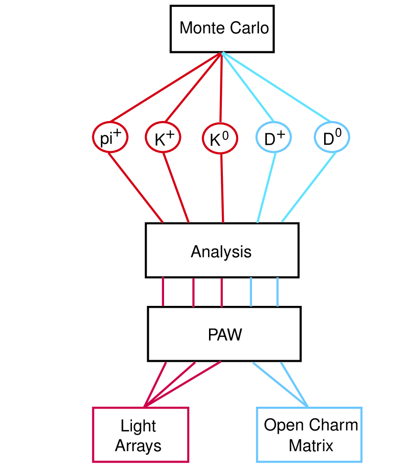
Several major modifications were made to the Monte Carlo to simulate single muon decays from the hadrons of interest. The event generator was modified to throw the desired hadrons using a distribution flat in $p_{T}\left(h\right)$, center of mass rapidity, $y$, and $\phi$. Once the hadron was thrown the event generator was required to determine a decay point based on the decay properties of the hadron and its momentum. Traversal of target or dump materials and magnetic field effects of the spectrometer magnet SM12 were simulated in a new section of the program for all charged hadrons. Hadron decay was performed using a CERN routine named GENBOD, and all decay products were transformed to the lab frame using the CERN routine LORENB. Secondary hadron decays, when required, were introduced by repeating the hadron tracing and decay sections for each secondary hadron of interest resulting from the primary hadron decay. These modifications allowed for large numbers of events at high transverse momentum since all hadrons that made it into the spectrometer were allowed to decay, and all hadrons were thrown flat in $p_{T}\left(h\right)$. Figure 4.2 shows a representation of the single muon Monte Carlo process.

Figure 4.2: Basic outline of the Monte Carlo process to calculate the various contributions to the single muon spectra.

Various cuts on primary hadrons, secondary hadrons and decay muons were implemented throughout the event generator and muon tracing sections of the Monte Carlo. The first set of cuts were loose aperture and momentum cuts taken on the hadrons immediately after they were thrown and histogrammed. This increased the efficiency of the Monte Carlo since similar or harder cuts on the thrown hadron were done later while the hadron was being traced through the spectrometer magnet. All decay muons or secondary hadrons having $|\overrightarrow{p}|\leq 50$ GeV/c were cut immediately after the decay and boost routines were done. All hadrons that were allowed to contribute secondary muons that resulted in more than one muon traversing the spectrometer were cut. A cut was imposed on all muons that tracked through any of the pulled x hodoscopes.

After a muon had passed all cuts the parent hadron and decay muon information required for producing weighted spectra was written to the MC data file.

4.1 Weighted Spectra

Extraction of the open charm cross sections required a set of $p_{T}\left(\mu\right)\;$spectra from all hadrons contributing to the data. These spectra were required to be the muon spectra that would result for a given number of protons interacting in the various materials of the targets and copper dump. A set of weights were given each muon as it was written to disk. These weights are shown in Table 4.1. The total weight of a muon is the product of the individual weights (listed in Table 4.1) appropriate for the event.

Table 4.1: Weights calculated for muons in the Monte Carlo spectra. Hadrons are divided into groups, light ($L$), open charm ($H$) and both ($B$). $E\,\frac{d^{3}\,\sigma}{d\,p^{3}}\;(mb\,c^{3}\,GeV^{-2})$ is the p-p  differential cross section at the thrown $p_{T}\left(h\right)\;$and c.m. $y$ of the hadron, $A^{\alpha{\left(p_{T}\left(h\right)\right)}}$ is the nuclear dependency of the hadron, $P_{D}$ is the probability that the hadron has decayed in the spectrometer,$P_{NA}$ is the likelihood that a hadron produced in the target did not interact in any remaining material in the target and $br(mode)$ is the muonic branching fraction of the decay mode.

Weight		Hadron
$W_{x}$	$E\,\frac{d^{3}\,\sigma}{d\,p^{3}}\;(mb\,c^{3}\,GeV^{-2})$	$L$
$W_{A}$	$A^{\alpha\left(p_{T}\left(h\right)\right)}$	$L$
$W_{D}$	$P_{D}$	$B$
$W_{NA}$	$P_{NA}$	$B$
$W_{br}$	$br\left(mode\right)$	$B$

4.1.1 The Light Hadron p-p  Cross Section Weight

All hadron distributions were parameterized using p-p  differential cross sections, and the following experimentally determined relationship was used to convert those cross sections to p-A  cross sections:

$$E\frac{d^{3}\sigma^{pA}(h)}{dp^{3}}=A^{\alpha(h,p_{T}\left(h\right))}\;E\,\frac{d^{3}\sigma^{\textit{p-p}\;}(h)}{dp^{3}}\qquad\mbox{(mb c${}^{3}$ GeV${}^{-2}$) \,}$$ (4.1)

where $h$ is the hadron of interest and $A^{\alpha(h,p_{T}\left(h\right))}$ is referred to as the nuclear dependency term.

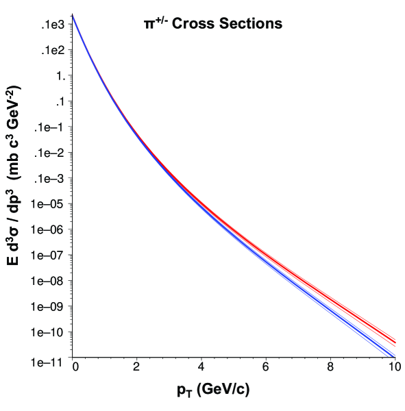
A parameterization of the p-p  differential $\pi^{\pm}\;$and $K^{\pm}\;$cross sections as a function of transverse momentum, $p_{T}\left(h\right)$, and c.m. rapidity $y$, developed by the British-Scandinavian Collaboration (BSC) at CERN [32] was used to calculate the cross section weight, $W_{x}$ (mb c³ GeV^-2)  . The parameterization of the differential cross sections developed by the BSC is

$$E\,\frac{d^{3}\,\sigma^{\textit{p-p }}(h)}{dp^{3}}(p_{T}\left(h\right),y)=A_{1}\,e^{\left(-B\,p_{T}\left(h\right)\right)}\,e^{\left(-Dy^{2}\right)}+A_{2}\frac{\left(1-\frac{p_{T}\left(h\right)}{p^{cm}_{beam}}\right)^{m}}{\left(p_{T}\left(h\right)^{2}+M^{2}\right)^{n}}$$ (4.2)

where values for the parameters $A_{1}$, $B$, $D$, $A_{2}$, $M$, $m$ and $n$ suggested for use by the BSC, their best central value and undertainty are listed in Table 4.2. It should be noted that the exponent $n$ was held fixed at 4 for all fits, and the collaboration suggested no deviation for that parameter. The center-of-mass (c.m.) momentum of the proton, $p^{cm}_{beam}$, introduces the energy dependency of hadron production and for this experiment was set to $p^{cm}_{beam}=19.37$ GeV/c.

It was assumed that $\sigma(K^{0})+\sigma(\overline{K}^{0})=\sigma(K^{+})+\sigma(K^{-})$ and that a similar production relationship existed between the $K^{0}\;$and $\overline{K}^{0}\;$as between the $K^{+}\;$and $K^{-}\;$due to conservation of isospin. This was introduced into the Monte Carlo by using $\sigma(K^{0})=\sigma(K^{+})$ and $\sigma(\overline{K}^{0})=\sigma(K^{-})$. The Monte Carlo did not throw $K^{0}\,/\,\overline{K}^{0}\;$but instead threw $K_{L}$ where the parent was either a $K^{0}\;$(50%) or $\overline{K}^{0}\;$(50%).

Table 4.2: Values of the parameters used in the BSC parameterization of the $\pi^{\pm}\;$and $K^{\pm}\;$differential cross sections. Fits were to data with $p_{T}\;$between 0 and approximately 6 GeV/c. Taken from [32].

	$A_{1}$	$B$	$D$	$A_{2}$	$M$	$m$
$\pi^{+}\;$	$210\pm 4$	$7.58\pm 0.11$	$0.20\pm 0.01$	$10.7\pm 0.7$	$1.03\pm 0.03$	$10.9\pm 0.4$
$\pi^{-}\;$	$205\pm 4$	$7.44\pm 0.09$	$0.21\pm 0.01$	$12.8\pm 0.9$	$1.08\pm 0.02$	$13.1\pm 0.4$
$K^{+}\;$	$14.3\pm 0.4$	$6.78\pm 0.21$	$1.5\pm 0.1$	$8.0\pm 1.1$	$1.29\pm 0.03$	$12.1\pm 0.8$
$K^{-}\;$	$13.4\pm 1.0$	$6.51\pm 0.23$	$1.8\pm 0.1$	$9.8\pm 1.7$	$1.39\pm 0.04$	$17.4\pm 1.0$

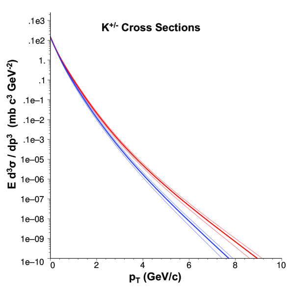
Figures 4.3 and 4.4 show the $\pi^{\pm}\;$and $K^{\pm}\;$cross sections for the parameterizations in [32] at $y=0$ (c.m.) for the energy of this experiment, $\sqrt{s}=38.8$ GeV.

Figure 4.3: The $\pi^{+}\;$(red) and $\pi^{-}\;$(blue) differential cross section as used in the Monte Carlo. Distribution is taken at c.m. $y=0$ and $p^{cm}_{beam}=19.37$ GeV/c. The value of the differential cross section at the thrown $p_{T}\left(h\right)\;$and $y$ was calculated and passed to the output MC data file and later used as a weight ($W_{x}$) for the event.

Figure 4.4: The $K^{+}\;$(red) and $K^{-}\;$(blue) differential cross sections as used in the Monte Carlo. Distribution is taken at c.m. $y=0$ and $p^{cm}_{beam}=19.37$ GeV/c. The value of the differential cross section for the thrown $p_{T}\left(h\right)\;$and $y$ was calculated for each event and passed to the output MC data file and later used as a weight ($W_{x}$) for the event.

4.1.2 Nuclear Dependency Term

It is well known that the proton-nucleus (p-A) cross section, at least for light hadrons, does not scale to the proton-proton (p-p ) cross section by the number of nucleons, $A$, in the target nucleus. The Chicago-Princeton Collaboration (C-P) studied the production of light hadrons on various nuclear targets and developed what has become known as the nuclear dependency term, relating the p-A  to p-p  cross sections by the relation [33]:

$$E\,\frac{d^{3}\,\sigma^{\mbox{pA}}}{d\,p^{3}}\left(p_{T}\right)=A^{\alpha(h,p_{T}\left(h\right))}\,E\,\frac{d^{3}\,\sigma^{\mbox{pp}}}{d\,p^{3}}\left(p_{T}\right)$$

where $A$ is the nuclear number (referred to as the atomic weight in [33] and $h$ is the species of hadron.

Light hadrons thrown in the Monte Carlo had the nuclear dependency calculated as a weight, $W_{A}$, that was passed to the Monte Carlo data files for use in weighting the thrown spectra after analysis. Since the open charm cross sections were determined as the p-Cu  and p-Be  cross sections, no nuclear dependency for the production of open charm was used.

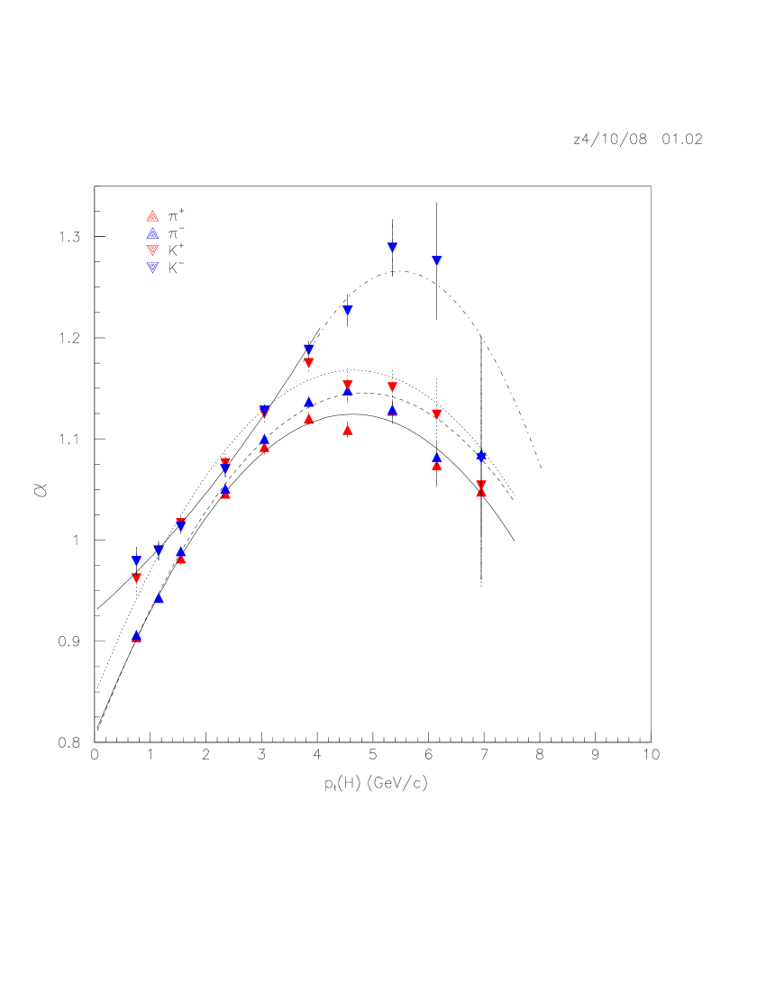
Data points from the Chicago-Princeton Collaboration (C-P) study for the nuclear number (or equivalently the atomic-weight) dependency for charged pion and kaon production from 400 GeV/c p-A  collisions [34] were fitted to simple quadratic equations of the form $p_{1}+p_{2}\,p_{T}+p_{3}\,p_{T}^{2}$ using the CERN program MINUIT. The resulting parameterizations were used to calculate the value of the dependency for each light hadron thrown. Figure 4.5 shows the four fits to the C-P data, and Table 4.3 gives the parameter values of the fits. The $K^{-}\;$parameterization was fitted to two regions in $p_{T}\left(h\right)$.

Table 4.3: Values for parameters of the equation $\alpha(h,p_{T}\left(h\right))=p_{1}+p_{2}\,p_{T}+p_{3}\,p_{T}^{2}$. The $K^{0}\;$used the same parameter values as the $K^{+}\;$and the $\overline{K}^{0}\;$used the same values as the $K^{-}$. The $K^{-}\;$fit required using two regions; hadrons thrown with transverse momentum less than 4.0 GeV/c, and hadrons having transverse momentum greater than 4.0 GeV/c.

	$p_{1}$	$p_{2}$	$p_{3}$
$\pi^{+}$	0.8074 $\pm$ 0.0072	0.1368 $\pm$ 0.0060	-0.0148 $\pm$ 0.0010
$\pi^{-}$	0.8043 $\pm$ 0.0059	0.1412 $\pm$ 0.0040	-0.0146 $\pm$ 0.0005
$K^{+}$	0.8464 $\pm$ 0.0154	0.1380 $\pm$ 0.0113	-0.01481 $\pm$ 0.0019
$K^{-}$	0.9295 $\pm$ 0.0148	0.0477 $\pm$ 0.0121	0.0053 $\pm$ 0.0006
	0.3649 $\pm$ 0.0654	0.3289 $\pm$ 0.0266	-0.0300 $\pm$ 0.0032

Figure 4.5: Fits of quadratic equations to the atomic-weight dependency for light hadrons. Data points taken from [34].

4.1.3 Probability To Decay

All hadrons thrown were given a weight, $W_{D}$, based on the likelihood that the hadron would decay, $L_{D}$, in the spectrometer. Since all hadrons must traverse some material, the loss of hadrons due to catastrophic collisions was included in the decay likelihood.

The probability for a hadron with momentum $|\overrightarrow{p}|\;$to decay in a distance $z$ is given by

$$P_{D}=1-exp\,\left(-z\,\frac{m}{p\,\tau}\right)$$ (4.3)

where $z$ is the distance the hadron has travelled (cm), $m$ is the mass of the hadron (GeV/c²), $p$ is the momentum (GeV/c) and $\tau$ is the proper lifetime (sec). The probability for a hadron to interact after traversing a distance $z$ in a material is calculated from

$$P_{I}=1-exp\,\left(-z\frac{\rho}{\lambda_{I}}\right)$$ (4.4)

where $\rho$ is the density of the material being traversed (gm cm^-3) and $\lambda_{I}$ (gm cm^-2) is the nuclear interaction length of the material for the hadron, which is slightly dependent on the hadron momentum. The two processes are independent of each other, so the likelihood that a hadron has neither interacted nor decayed in a length $z$ and will decay in the next differential thickness $dz$ is given by

$$\frac{dP_{D}}{dz}=\frac{m}{p\,\tau}\,exp\left[-z\left(\frac{m}{p\,\tau}+\frac{\rho}{\lambda_{I}}\right)\right]$$ (4.5)

The fraction of hadrons that will decay while traversing a material is found by integrating Equation 4.5 and normalizing the result such that the likelihood for a hadron to either decay or interact while traversing a target of infinite thickness is unity. The fraction of hadrons that will decay while traversing a material of thickness $z$ is then given by

$$F_{D}=\frac{m\,\lambda_{I}}{m\,\lambda_{I}+\rho\,p\,\tau}\,exp\left[-z\left(\frac{m}{p\,\tau}+\frac{\rho}{\lambda_{I}}\right)\right]$$ (4.6)

while the fraction that will interact, $F_{I}$, is given by

$$F_{I}=\frac{\rho\,p\,\tau}{m\,\lambda_{I}+\rho\,p\,\tau}\,exp\left[-z\left(\frac{m}{p\,\tau}+\frac{\rho}{\lambda_{I}}\right)\right]$$ (4.7)

The fraction of hadrons not interacting while traversing a material, $F_{NI}=1-F_{I}$ was more useful in calculating the likelihood for decay in the spectrometer.

The assumption was made that all hadrons traversing the dump would either interact or decay, so the length of the dump was set to infinity in Equation 4.6 for simplicity. This assumption reduced Equation 4.6 to

$$F_{D}=\frac{m\,\lambda_{I}}{m\,\lambda_{I}+\rho\,p\,\tau}$$

. It was also assumed that all open charm hadrons thrown from the target would decay if they didn’t interact while traversing any remaining material in the target.

The likelihood that the hadron thrown would decay in the spectrometer was then determined as follows:

• If a light hadron was thrown in the target, the likelihood for decay was calculated using

  $$W_{D}=F_{NI}\,P_{D}+\left(1-F_{NI}\,P_{D}\right)\,F_{D}$$

• If an open charm hadron was thrown in the target, then

  $$W_{D}=F_{NI}$$

• All hadrons thrown in the dump used

  $$W_{D}=F_{D}$$

In all cases, the value of $F_{NI}$ used the difference between the thickness of the target and the $z$ location where the hadron was produced (Section 4.1.4 below), and the distance used in calculating $P_{D}$ was set to 92 inches (233.68 cm), the distance between the targets and the beam dump.

The nuclear interaction length, $\lambda_{I}$, for light hadrons was calculated using the results published by A. S. Carrol, et al. [35]. The code initialized three interaction lengths associated with three momentum ranges of the hadron, $0<p_{T}\;\leq 130$, $130<p_{T}\;\leq 240$ and $p_{T}\;>240$ GeV/c. The nuclear interaction length, calculated using the absorption cross sections determined by A. S. Carroll, et al., are given in Table 4.4. The nuclear interaction lengths for open charm was calculated by decreasing the absorption cross section for strange particles by 10 percent.

Table 4.4: Absorption cross section, $\sigma_{a}$, and nuclear interaction length, $\lambda_{I}$, for hadrons thrown in the Monte Carlo. All hadron momenta are in GeV/c. Nuclear interaction length for neutral kaons and $D^{0}\,/\,\overline{D}^{0}\;$are the same as their charged counterparts. The density for beryllium used was 1.848 gm cm^-3, and for copper 8.96 gm cm${}^{-3}\;$. The nuclear interaction lengths for protons was taken directly from the tables provided by the Particle Data Group.

$H$	$p_{T}\;$	Copper		Beryllium
	Range	$\sigma_{a}$ (mb)	$\lambda_{I}$ gm cm${}^{-2}\;$	$\sigma_{a}$ (mb)	$\lambda_{I}$ gm cm${}^{-2}\;$
$\pi^{+}\;$	$0\,-\,130$	$611.6\pm 34.8$	$172.5\pm 9.8$	$137.5\pm 6.2$	$108.8\pm 4.9$
	$130\,-\,240$	$616.6\pm 35.2$	$171.0\pm 9.8$	$139.3\pm 6.2$	$107.4\pm 4.8$
	$>\,240$	$608.6\pm 37.0$	$173.4\pm 10.5$	$140.4\pm 6.6$	$106.6\pm 5.0$
$\pi^{-}\;$		$611.8\pm 34.7$	$172.5\pm 9.8$	$138.1\pm 6.1$	$108.4\pm 4.8$
		$611.4\pm 34.7$	$172.6\pm 9.8$	$138.8\pm 6.2$	$107.8\pm 4.8$
		$610.6\pm 36.6$	$172.8\pm 10.4$	$139.7\pm 6.4$	$107.1\pm 4.9$
$K^{+}\;$		$543.5\pm 31.1$	$194.1\pm 11.1$	$115.9\pm 5.2$	$129.1\pm 5.8$
		$562.7\pm 32.3$	$187.5\pm 10.8$	$122.2\pm 5.5$	$122.5\pm 5.6$
		$555.8\pm 36.8$	$189.9\pm 12.6$	$122.3\pm 6.2$	$122.3\pm 6.2$
$K^{-}\;$		$572.7\pm 33.0$	$184.2\pm 10.6$	$125.1\pm 5.7$	$119.7\pm 5.5$
		$571.3\pm 32.8$	$184.7\pm 10.6$	$125.2\pm 5.7$	$119.5\pm 5.4$
		$570.0\pm 35.6$	$185.1\pm 11.6$	$126.4\pm 6.2$	$118.4\pm 5.8$
$D^{+}\;$			$215.7\pm 12.3$		$143.4\pm 6.5$
			$208.4\pm 12.0$		$136.1\pm 6.2$
			$211.0\pm 14.0$		$135.9\pm 6.9$
$D^{-}\;$			$204.7\pm 11.8$		$133.0\pm 6.1$
			$205.2\pm 11.8$		$132.8\pm 6.0$
			$205.7\pm 12.9$		$131.5\pm 6.4$
$p$			$134.9$		$75.2$

4.1.4 Proton Interaction And Hadron Decay Distributions

Two routines were used to model the distribution of hadron interactions in the materials; one using a two dimensional Gaussian distribution to model the axial dispersion of the proton beam, and one using a distribution based on the likelihood that a hadron had not interacted in a randomly chosen distance. As before, the distance along the $z$ axis was used as the total distance ignoring any small $x$ or $y$ components. The beam distribution was provided in the original Monte Carlo. All lengths and distances throughout this section are in cm.

All hadrons thrown assumed that a proton-nucleon interaction had occured, and that all hadrons would decay (the decay weight, $W_{D}$, described in 4.1.3 above provided the proper scaling for loss due to interactions). The Monte Carlo used an iterative process where a trial distance in the material at which the interaction or decay would occur $(\Delta_{z}$, and then tested the trial distance against the interaction or decay distribution. If the trial distance fell within the distribution, the routine then determined the point $(\Delta_{x},\Delta_{y},\Delta_{z})$ at which the decay or interaction would have occured based on either the distributed beam diffusion and beam correction angles, or the momentum of the hadron $\overrightarrow{p}$. If the trial distance failed to fall within the distribution, the routine initiated a new trial $\Delta_{z}$ until a distance was accepted.

Specifically, to determine the point along the $z$ axis at which the proton had interacted for hadrons thrown from the target, the routine threw a random number (all random numbers were between 0 and 1) and multiplied the number to the thickness of the target, providing the trial interaction distance, $\Delta_{z}$. The likelihood that the proton had survived to the trial distance was calculated using:

$$L_{NI}=exp\,\left(-\Delta_{z}\,\frac{\rho_{A}}{\lambda_{I}(p,A)}\right)$$

where $\rho_{A}$ (gm cm^-3) is the density of the target material $A$ and $\lambda_{I}(p,A)$ (gm cm^-2) is the nuclear interaction length for 800 GeV/c protons in the material. $L_{NI}$ was referred to as the test function. A second random number, $rn$ was thrown and compared to the value $L_{NI}$. If $rn\leq L_{NI}$ the trial distance $\Delta_{z}$ was accepted and the routine then determined the interaction point $(X_{I},Y_{I},Z_{I})$ where $X_{I}=\delta_{x}+XSLP\,\Delta_{z}$. $\delta_{x}$ was the distance in $x$ away from the $z$ axis determined by the beam dispersion routine, and XSLP is the beam angle in the $x-z$ plane defined in 3.4.2. If $rn>L_{NI}$, the process was repeated until the test distance $\Delta_{x}$ was accepted. $Y_{I}$ was calculated by substituting $y$ for $x$, and $Z_{I}=-60.96+\Delta_{z}$.

For hadrons thrown in the dump, the process to determine where the proton interacted was the same, except the trial distance was limited to the distance at which 95 percent of the proton interactions would have occured, and magnetic field effects were included. The maximum distance $\Delta^{max}_{z}$ was calculated using

$$\Delta^{max}_{z}=-\,ln(0.05)\,\frac{\lambda_{I}(p,Cu)}{\rho_{Cu}}$$

The trial distance was then calculated using $\Delta_{z}=rn\,\Delta^{max}_{z}$. Once a $z$ decay distance had been found, the routine projected the proton through the spectrometer to the point $Z_{I}=203.2+\Delta_{z}$. The proton was given initial $\delta_{x}$ and $\delta_{y}$ components as well as the correct beam angle before the projection was performed, so the interaction point, $(X_{I},Y_{I},Z_{I})$, was the values of the position of the proton at $Z_{I}$ after the projection.

The distribution of hadron decays for hadrons produced in the dump were handled in the much the same manner. The test function used was

$$L_{NI}=exp\left[-z\left(\frac{m}{p\,\tau}+\frac{\rho_{Cu}}{\lambda_{I}(h,Cu)}\right)\right]$$

where $m$ is the mass (GeV c^-2), $p$ the magnitude of the momentum $\overrightarrow{p}$(GeV/c), $\tau$ the proper lifetime (s) and $\lambda_{I}(h,Cu)$ the nuclear interaction length (gm cm^-2) of the hadron $h$. The maximum allowable distance, $\Delta^{max}_{z}$ was determined by setting $L_{NI}=0.05$ and solving for $z$.

Two test functions were required for light hadrons thrown from the dump, one for the distribution of decays in the open decay region between the target and the dump, and one for the distribution of decays in the dump if the hadron survived the open decay length. The test function used for $\Delta_{z}\leq 233.68$ (cm) was:

$$L^{odl}_{I}=exp\,\left(-z\,\frac{m}{p\,\tau}\right)$$

where $odl$ signifies the open decay length (233.68 cm). The test function for $233.68<\Delta_{z}\leq\Delta^{max}_{z}$ (cm) was given as

$$P^{odl}_{S}\,exp\left[-z\left(\frac{m}{p\,\tau}+\frac{\rho_{Cu}}{\lambda_{I}(h,Cu)}\right)\right]$$

where $P^{odl}_{S}=1-exp\,\left[\left(-233.68\,m\right)\,/\,\left(p\,\tau\right)\right]$ (the probability the hadron did not decay in the open decay region) and $\Delta^{max}_{z}$ was calculated by setting $L_{NI}=0.05$ in the second test function and solving for $z$ and adding 233.68 (cm). Figure 4.6 shows a plot of the two test functions used to determine the decay distribution of charged kaons having $|\overrightarrow{p}|=55.0$ GeV/c.

Figure 4.6: The two test functions used to determine the decay distribution for 55.0 GeV/c charged kaons thrown from a target. The value of the test function at the randomly chosen decay distance was compared to a random number between 0 and 1. If the random number was smaller than or equal to the value of the test function, the decay distance was accepted, if not a new decay distance was calculated and the process repeated until a distance met the required test. Distance is the distance downstream of the target ($Z_{tgt}=-60.96$ cm)

4.1.5 Decay Modes And Branching Fractions

The Monte Carlo used a set of decay mode routines to determine the mode and branching fraction of the mode chosen. Since the Monte Carlo spectra were weighted spectra, only semi-muonic decay modes were allowed for open charm hadrons. Table 4.5 shows the decay modes allowed for each hadron species thrown in the Monte Carlo. The weight given each decay was the branching fraction listed. Strange hadrons were allowed to decay to charged pions, which were subsequently passed through the decay routine as secondary decays. However, if more than one muon was accepted the event was cut due to the requirement in the analysis section where only one valid track was allowed for each event.

Table 4.5: The decay modes allowed in the Monte Carlo. The weight $W_{br}$ given any muon that was accepted was the branching fraction as shown. Only the hadron decay modes are shown, the anti-hadron modes are the charge conjugate of the mode listed. The $K_{L}$ hadrons were assumed to be from $K^{0}\;$50 percent of the time, and $\overline{K}^{0}\;$50 percent of the time. Decay modes of the anti-hadrons are the charge conjugate of those shown.

	Decay	Branching
Hadron	Mode	Fraction
$\pi^{+}$	$\mu^{+}\,\nu_{\mu}$	1.0000
$K^{+}$	$\mu^{+}\,\nu_{\mu}$	0.6351
	$\pi^{0}\,\mu^{+}\,\nu_{\mu}$	0.0318
	$\pi^{+}\,\pi^{0}$	0.2116
	$\pi^{+}\,\pi^{+}\,\pi^{-}$	0.0559
	$\pi^{+}\,\pi^{0}\,\pi^{0}$	0.0173
$K_{L}$	$\pi^{\pm}\;\mu^{\mp}\nu$	0.2717
	$\pi^{+}\,\pi^{-}\,\pi^{0}$	0.1256
	$\pi^{\pm}\,e^{\mp}\,\nu_{e}$	0.3878
$D^{+}$	$\mu^{+}\,\nu_{\mu}\,\overline{K}^{0}$	0.0650
	$\mu^{+}\,\nu_{\mu}\,\overline{K}^{*}(892)^{0}$	0.0440
	$\mu^{+}\,\nu_{\mu}\,\phi$	0.0370
	$\mu^{+}\,\nu_{\mu}\,\overline{K}_{1}(1270)^{0}$	0.0350
$D^{0}\;$	$\mu^{+}\,\nu_{\mu}\,K^{-}$	0.0343
	$\mu^{+}\,\nu_{\mu}\,\overline{K}^{*}(892)^{-}$	0.0214
	$\mu^{+}\,\nu_{\mu}\,{K}^{-}\,\pi^{0}$	0.0031

Chapter 5 Method Used To Extract The Open Charm Cross Sections

This analysis used the single muon data and Monte Carlo muon spectra to extract four inclusive open charm differential cross sections, $E\,\frac{d^{3}\,\sigma^{\mbox{\tiny{Cu}}}\left(D\right)}{d\,p^{3}}\left(p_{T}\right)$, $E\,\frac{d^{3}\,\sigma^{\mbox{\tiny{Cu}}}\left(\overline{D}\right)}{d\,p^{3}}\left(p_{T}\right)$, $E\,\frac{d^{3}\,\sigma^{\mbox{\tiny{Be}}}\left(D\right)}{d\,p^{3}}\left(p_{T}\right)\;$and $E\,\frac{d^{3}\,\sigma^{\mbox{\tiny{Be}}}\left(\overline{D}\right)}{d\,p^{3}}\left(p_{T}\right)\;$by fitting the Monte Carlo spectra to the data. The Monte Carlo spectra were referred to as total Monte Carlo spectra. The open charm contribution to a total Monte Carlo spectrum could be varied by using open charm differential cross sections parameterized by functions of the hadrons $p_{T}$. The open charm cross sections were fit to the data using a least-squares minimization routine where each data point contributed an individual $\chi^{2}\;$calculated as the square of the difference between the data and the total Monte Carlo spectrum for that data point, divided by the sum of the squares of the errors:

$$\chi^{2}_{j}=\frac{\left(N^{\mu}_{j}-W^{MC}_{j}\right)^{2}}{\varepsilon^{2}_{j}+\epsilon^{2}_{j}}$$ (5.1)

where $N^{\mu}_{j}$ is the number of muons from the data in a histogram bin $j$ and $W^{MC}_{j}$ is the number of muons determined from weighted spectra in bin $j$ of a histogram of the total Monte Carlo spectrum corresponding to the data. The errors $\varepsilon$ and $\epsilon$ are the errors for the data and composite Monte Carlo, respectively.

Use of single muons prevented the analysis from determining which species of hadron decayed to a given muon. In the case of open charm production, hadrons containing a charm quark and a light anti-quark $\left(c,\overline{q}\right)\;$are designated $D$ , and those having an anti-charm quark and a light quark $\left(q,\overline{c}\right)\;$are designated by $\overline{D}$. The inclusive $D\;$cross sections were extracted using $\mu^{+}\;$spectra, and the inclusive $\overline{D}\;$cross sections were extracted using $\mu^{-}\;$spectra.

Previous experiments have fitted various functions to their results based on theoretical predictions of the shape of the spectra as a function of $p_{T}\left(h\right)\;$. From the literature, the functions used to parameterize the open charm cross sections for this analysis were:

$$A_{1}\,exp\left(-B\,p_{T}\right)\;$$ (5.2)

$$\frac{A_{2}}{\left(p_{T}^{2}+\alpha\,m_{c}^{2}\right)^{n}}\;$$ (5.3)

$$A_{2}\,\frac{\left(1-p_{T}\,/\,p_{beam}\right)^{m}}{\left(p_{T}^{2}+\alpha\,m_{c}^{2}\right)^{n}}\;$$ (5.4)

Another exponential form, $A_{1}^{\prime}\,exp\left(-B^{\prime}\,p_{T}^{2}\right)\;$, used in [8] and [9], was also attempted but resulted in very high total $\chi^{2}\;$indicating it should not be used to describe the open charm cross sections for this data. Function 5.2 is referred to as the exponential form and the functions 5.3 and 5.4 are referred to as the 3 and 4 parameter forms, respectively. There were 4 fits performed using $\frac{A_{2}}{\left(p_{T}^{2}+\alpha\,m_{c}^{2}\right)^{n}}\;$as the open charm cross sections, one where all parameters were free parameters, and one each where $n$ was held fixed at the integer values 4, 5 and 6. These were chosen from theoretical predictions as well as fits used in previous experiments [4], [9], [32], [36], [37], [38], [39], [40], [41]. Fits to $A_{2}\,\frac{\left(1-p_{T}\,/\,p_{beam}\right)^{m}}{\left(p_{T}^{2}+\alpha\,m_{c}^{2}\right)^{n}}\;$were done for the same fixed values of $n$ only. All fits using the 3 and 4 parameter functions used $m_{c}=1.5$ GeV c^-2. The 4 parameter function includes an energy dependency term, $\frac{p_{T}\left(h\right)}{p_{beam}}$ where $p_{beam}$ is the center of mass momentum of the proton beam. For this experiment, $p_{beam}=19.36$ GeV/c.

Each target provided four independent but related muon spectra; $\mu^{+}\;$and $\mu^{-}\;$from interactions in the target, and $\mu^{+}\;$and $\mu^{-}\;$from interactions in the dump. All four spectra were related by the number of protons incident on the target. Each fit required four total Monte Carlo spectra to be compared against the four data spectra simultaneously.

A total Monte Carlo spectrum is the number of muons resulting from $2\times 10^{7}$ proton interactions in either copper or beryllium. More precisely, the total Monte Carlo copper target $\mu^{+}\;$spectrum is the number of $\mu^{+}\;$resulting from the interactions of $2\times 10^{7}$ protons in the copper target. The spectrum was determined from adding the number of $\mu^{+}\;$from light hadron production, called the light contribution, plus the number of $\mu^{+}\;$resulting from production of open charm, called the open charm contribution. The light contribution is the sum of the muons from the production of $\pi^{+}$, $K^{+}\;$and $K^{0}/\overline{K}^{0}\rightarrow K_{L}\rightarrow\mu^{+}$ copper target Monte Carlo spectra. The light contributions were normalized since all the light hadrons were thrown using fully normalized differential cross sections. The open charm contribution was calculated using a set of values for the free parameters of the function being fitted.

The four data spectra were related by the total number of incident protons, $N_{p}$. The Monte Carlo generated all spectra using $2\times 10^{7}$ incident protons, so a scaling factor $N$ was introduced to scale the total MC spectra to the proper number of incident protons. The spectrometer lacked a beam intensity monitor which was sensitive to the requested number of protons per spill, so the parameter $N$ (referred to as the scale factor $N$) was introduced as an extra free parameter for all fits. The relationship between $N$ and $N_{p}$ is given in section 5.2. The requirement that the four data and four total MC spectra be used in calculating $\chi^{2}$, and the use of normalized light contributions resulted in normalized open charm cross sections. Figure 4.2 (page 4.2) shows a representation of the process used to calculate the light MC contributions and the open charm transformation arrays used to extract the open charm cross sections. The open charm arrays and their use are described in Chapter 5.3. For reference, Figure 3.1 (Chapter 3 page 3.1) shows the method used to analyze the single muon data and place the resulting muon spectra into arrays used in the least-squares minimization routines.

Figure 5.1 shows the $\mu^{+}\;$spectra for the individual and the light Monte Carlo contribution used for all fits for the copper target (top left) and dump (lower left). The upper and lower right histograms show the light Monte Carlo contribution scaled to the data after the 3 parameter function with $n$ a free parameter had been fitted. Figure 5.2 shows the $\mu^{+}\;$data (black circles), total Monte Carlo $\mu^{+}\;$spectra (blue open squares) and the open charm Monte Carlo $\mu^{+}\;$contribution (red open circles) for the open charm cross section determined from the fit in Figure 5.1. Left is the spectra for the copper target and right is the dump.

Figure 5.1: Left Figures: light Monte Carlo $\mu^{+}\;$contribution (black filled circles) from the copper target (top) and beam dump (bottom), composed of the sum of $\mu^{+}\;$spectra from $\pi^{+}$ (red open circles), $K^{\pm}$ (blue open squares) and $K^{0}\,/\,\overline{K^{0}}$ (green open triangles). Right Figures: the same light Monte Carlo contribution after fitting the 3 variable function with $N$ a free parameter (red open circles) and the $\mu^{+}\;$data (black closed circles). Errors are statistical only for the figures on the left. For figures on the right, the errors for the data are statistical only, the scaled light MC contributions have all systematic errors except normalization added in quadrature to the statistical errors.

Figure 5.2: Total open charm Monte Carlo $\mu^{+}\;$contribution (blue open squares), total light MC $\mu^{+}\;$spectra from Figure 5.1 (red open circles) and the the data (black filled circles) from the copper target (left) and the dump (right). Data is the $\mu^{+}\;$spectra from the copper target, and the Monte Carlo spectra are from fitting the 3 variable function with $n$ a free parameter. Data errors are statistical only. MC spectra have all systematic errors except normalization added in quadrature to the statistical error.

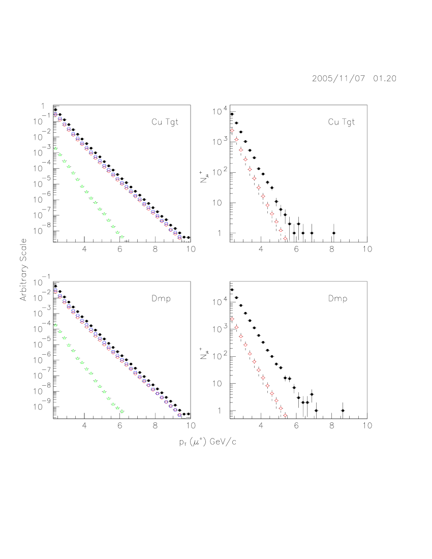
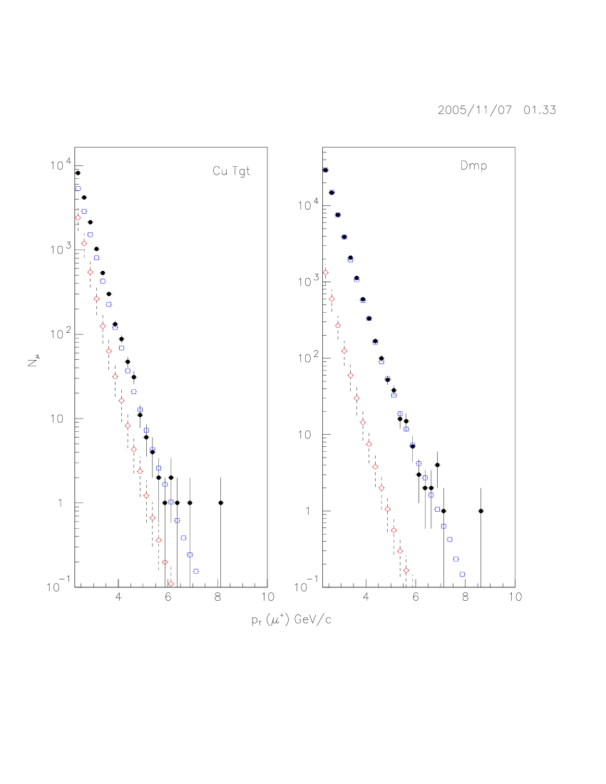
5.1 Minimization

The three parameterizations of the open charm differential cross sections used in this analysis were:

$$A_{1}\,exp\left(-B\,p_{T}\right)\;$$

$$\frac{A_{2}}{\left(p_{T}^{2}+\alpha\,m_{c}^{2}\right)^{n}}\;$$

$$A_{2}\,\frac{\left(1-p_{T}\,/\,p_{beam}\right)^{m}}{\left(p_{T}^{2}+\alpha\,m_{c}^{2}\right)^{n}}\;$$

The analysis histogrammed the data into 1-dimensional histograms with 40 bins from 0 to 10 GeV/c in $p_{T}$. The contents of the bins in the histograms were placed into arrays for use in minimization. The light Monte Carlo spectra were placed into similar arrays, and the contents of $p_{T}\left(\mu\right)\;$versus $p_{T}\left(h\right)\;$histograms were placed into 40 $\times$ 40 2-dimensional arrays, referred to as hadron to muon $p_{T}\;$transformation arrays.

A change in any free parameter resulted in four total MC spectra to compare against the data. A $\chi^{2}\;$, called an individual $\chi^{2}\;$, $\chi^{2}_{j}$, was calculated for all data points in the four data spectra using Equation 5.1 (page 5.1). The total $\chi^{2}\;$, $\chi^{2}_{tot}$, was the sum of the individual $\chi^{2}\;$:

$$\chi^{2}_{tot}=\sum_{j=1}^{k}\chi^{2}_{j}$$ (5.5)

where $k$ is the total number of elements in the four data arrays containing three or more muons.

The spectrometer had the middle half of all x measuring hodoscope layers pulled, creating two inner acceptance edges (see Figure 2.4 page 2.4). These acceptance edges combined with the single bend approximation used to correct for multiple scattering resulted in large uncertainties in muon $p_{T}\;$below 2.25 GeV/c. Attempts to correct this uncertainty failed because no decay vertex was available. As a consequence, the fits were limited to $p_{T}\left(\mu\right)\geq 2.25$ GeV/c.

The minimization routines used a grid search method to insure that local minima were avoided. The routines fitted each cross section individually in a rotating sequence. Normal initialization began with fitting the hadron cross section, $E\,\frac{d^{3}\,\sigma\left(D\right)}{d\,p^{3}}\left(p_{T}\right)$, while the anti-hadron cross section, $E\,\frac{d^{3}\,\sigma\left(\overline{D}\right)}{d\,p^{3}}\left(p_{T}\right)$, remained constant using a set of initial parameter values. Once a set number of passes through the grid search had been performed on the hadron cross section, the routine re-initialized to begin fitting the anti-hadron cross section holding the hadron cross section constant at the values of the parameters that returned the smallest total $\chi^{2}\;$(referred to as $\chi^{2}_{min}$) during its fit. The scale factor $N$ was allowed to float freely during fits to either cross section, with the requirement that all four total Monte Carlo spectra be scaled by the same $N$ simultaneously at each point in the routine where $\chi^{2}_{tot}\;$was calculated.

Because the target and dump were the same material in the copper target data, fits to the p-Cu  data were performed first. Once the p-Cu  data had been fit to the various functions, and the $\chi^{2}_{min}\;$values of the parameters of the p-Cu  cross sections had been determined, fits of the p-Be  cross sections were performed to the two p-Be  target spectra. To accomplish this, the dump data were compared to scaled total Monte Carlo spectra calculated using a previous p-Cu  result. The open charm contributions from the dump for fits to the p-Be  data were calculated using the 4 parameter function with $n=6$ and the $\chi^{2}_{min}\;$values of the parameters found from the fit to the p-Cu  data. The scaling factor $N$ remained a free parameter.

5.2 Scaling Monte Carlo Spectra To The Target Material And Thickness

The Monte Carlo spectra needed to be scaled by the integrated luminosity Ł, before they could be compared against the data, where

$$\mbox{\L}_{tgt}=\frac{N_{p}\,N_{A}}{A}\,\lambda_{I}\,\left[1-exp\,\left(-l\,\rho\,/\,\lambda_{I}\right)\right]\qquad\left(\mbox{cm}^{-2}\right)$$

for the target spectra, and

$$\mbox{\L}_{dmp}=\frac{N_{p}\,N_{A}}{A}\,\lambda_{I}\,exp\,\left(-l\,\rho\,/\,\lambda_{I}\right)\qquad\left(\mbox{cm}^{-2}\right)$$

for the dump spectra where $N_{p}$ is the total number of protons incident on the target, $N_{A}$ (mole^-1) is the Avogadro constant, $\lambda_{I}$ (gm cm^-2) is the nuclear interaction length for protons in the material, $A$ (gm mole^-1) is the atomic weight of the material, $\rho$ (gm cm^-3) is the density of the material, and $l$ (cm) is the thickness of the target. The difference between the two is simply stating that all protons incident on the dump interacted in the dump, and the number of protons incident on the dump was the number incident on the target times the probability that the proton did not interact while traversing the target material. The target scaling includes loss of protons due to interactions in the target material.

It is important to note that $N_{p}$ is commmon to both. Since the experiment lacked a beam intensity monitor, the total number of protons incident on the target was unknown. To overcome this, the experiment split the total number of incident protons from the remaining terms of the two integrated luminosities such that $\mbox{\L}=N_{p}\,L$ where $L$ is

$$L_{tgt}=\frac{N_{A}}{A}\,\lambda_{I}\,\left[1-exp\,\left(-l\,\rho\,/\,\lambda_{I}\right)\right]\qquad\left(\mbox{cm}^{-2}\right)$$

for the target spectra, and

$$L_{dmp}=\frac{N_{A}}{A}\,\lambda_{I}\,exp\,\left(-l\,\rho\,/\,\lambda_{I}\right)\qquad\left(\mbox{cm}^{-2}\right)$$

for the dump spectra.

The minimization routine scaled the Monte Carlo spectra by the appropriate value of $L$ to match the data being fitted at initialization. To estimate the number of incident protons $N_{p}$, the total nuclear cross section weight thrown for p-Cu  $\pi^{+}\;$(either the target or dump) is divided by the total p-Cu  $\pi^{+}\;$cross section. The minimization routines input $N$ as a free parameter, and using the conversion from the thrown weight, $N_{p}\sim 21.42\times 10^{1}1\,N$. The $\chi^{2}_{min}\;$value for the parameter $N$ thus determined the integrated beam flux corrected for dead time.

5.3 Calculating The Open Charm Contributions

The open charm contribution to a total MC spectrum was calculated using an array whose elements, $\mathbf{W}^{D\rightarrow\mu}_{ij}$, were the weight of the muons having transverse momentum between 0.250$j$ and 0.250($j+1$) GeV/c, from open charm hadrons thrown with transverse momentum between 0.250$i$ and 0.250($i+1$) GeV/c. The array used for calculating the $\mu^{+}\;$spectrum from $D^{+}\;$and $D^{0}\;$produced in the copper target was composed of the elements

$$\mathbf{W}^{D\rightarrow\mu^{+}}_{ij}(T,Cu)=\mathbf{W}^{D^{+}\rightarrow\mu^{+}}_{ij}(T,Cu)+\mathbf{W}^{D^{0}\rightarrow\mu^{+}}_{ij}(T,Cu)$$

The Monte Carlo was used to develop a set of 6 arrays used to calculate the open charm contributions, one each $\mu^{+}\;$and $\mu^{-}\;$from the copper target, the beryllium target and the copper beam dump. The dump required only one set of arrays because the difference between the arrays from the dump with either target presented to the beam would be the target thickness normalization presented in Chapter 5.2. The elements of the arrays were the values of the weight in the bins of 2-dimensional $p_{T}\left(\mu\right)\;$versus $p_{T}\left(h\right)\;$histograms of the individual open charm hadrons thrown in the Monte Carlo. Figure 5.3 shows the 2-dimension $p_{T}\left(\mu\right)\;$versus $p_{T}\left(h\right)\;$histogram resulting from 20 million $D^{+}\;$and $D^{0}\;$thrown from the copper target. Table 5.1 gives the 12 individual arrays and the six transformation arrays used for calculating the open charm contributions.

Table 5.1: The six transformation arrays used in the minimization routines to determine the open charm contributions from the copper target ($Cu$), beryllium target ($Be$) and dump ($dmp$). The contribution is determined from the transformation array which is the sum of the weights of the two individual arrays listed, after an arbitrary open charm cross section is applied. A fit required four contributions to be determined for each change in any of the free parameters.

Spectrum	Transformation	Individual
Desired	Array	Array
		$\mathbf{W}^{D^{+}\rightarrow\mu^{+}}(Cu)$
$\mu^{+}(Cu)$	$\mathbf{W}^{D\rightarrow\mu^{+}}(Cu)$	$\mathbf{W}^{D^{0}\rightarrow\mu^{+}}(Cu)$
		$\mathbf{W}^{D^{-}\rightarrow\mu^{-}}(Cu)$
$\mu^{-}(Cu)$	$\mathbf{W}^{\overline{D}\rightarrow\mu^{-}}(Cu)$	$\mathbf{W}^{\overline{D}^{0}\rightarrow\mu^{-}}(Cu)$
		$\mathbf{W}^{D^{+}\rightarrow\mu^{+}}(Be)$
$\mu^{+}(Be)$	$\mathbf{W}^{D\rightarrow\mu^{+}}(Be)$	$\mathbf{W}^{D^{0}\rightarrow\mu^{+}}(Be)$
		$\mathbf{W}^{D^{-}\rightarrow\mu^{-}}(Be)$
$\mu^{-}(Be)$	$\mathbf{W}^{\overline{D}\rightarrow\mu^{-}}(Be)$	$\mathbf{W}^{\overline{D}^{0}\rightarrow\mu^{-}}(Be)$
		$\mathbf{W}^{D^{+}\rightarrow\mu^{+}}(dmp)$
$\mu^{+}(dmp)$	$\mathbf{W}^{D\rightarrow\mu^{+}}(dmp)$	$\mathbf{W}^{D^{0}\rightarrow\mu^{+}}(dmp)$
		$\mathbf{W}^{D^{-}\rightarrow\mu^{-}}(dmp)$
$\mu^{-}(dmp)$	$\mathbf{W}^{\overline{D}\rightarrow\mu^{-}}(dmp)$	$\mathbf{W}^{\overline{D}^{0}\rightarrow\mu^{-}}(dmp)$

Figure 5.3: The $p_{T}\left(\mu\right)\;$versus $p_{T}(D)$ histogram of Monte Carlo $D\rightarrow\mu^{+}\;$ used in the calculation of the muon contribution from D production from the copper target in the fitting routine. Weight does not include any cross section weight.

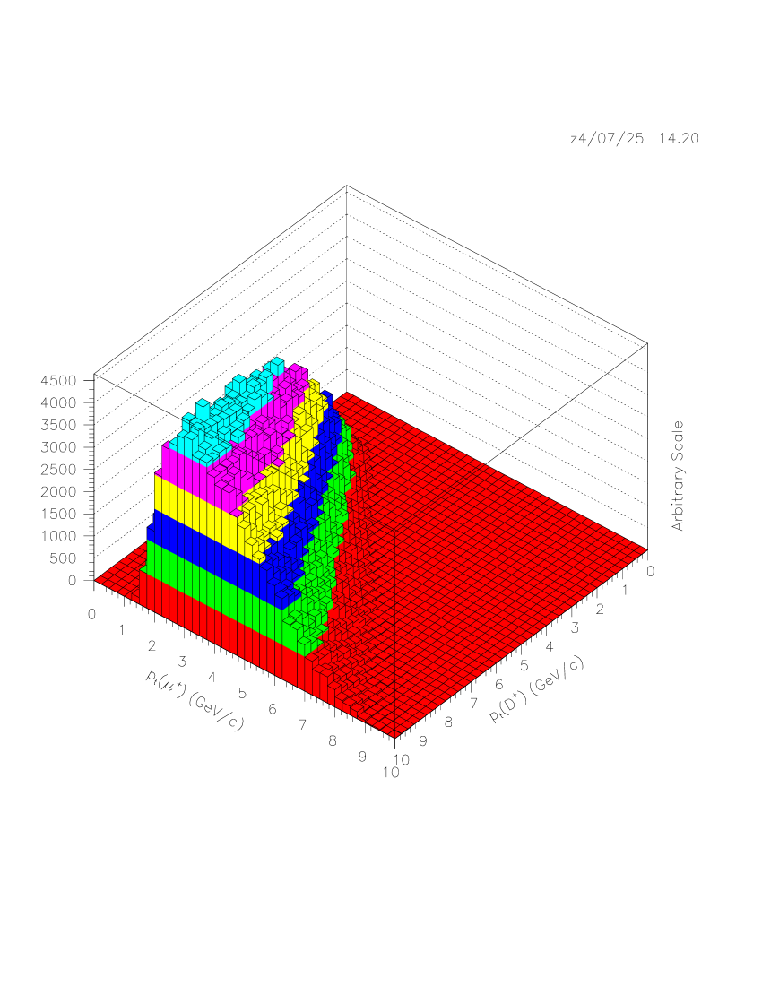
The value of an open charm (or anti-charm) cross section, $W^{D}_{x,i}$, was calculated at the center of each bin using $p_{T,i}=0.250\left(i-1\right)+0.125\quad(\mbox{GeV/c})$ for $i$ from 1 to 40. The muon spectrum expected from throwing the open charm hadrons with the cross section being tested was then determined by

$$W^{\mu}_{j}=\sum_{i=1}^{40}\left[W^{D}_{x,i}\,\mathbf{W}^{D\rightarrow\mu}_{i\,j}\right]$$

Figure 5.4 shows the result of applying a cross section weight for $D^{+}\;$to the histogram shown in Figure 5.3.

Figure 5.4: Same hadron to muon $p_{T}\;$distribution as in Figure 5.3 except trial input cross section weights $W^{\sigma(D)}_{i}$ have been calculated and applied to all columns $i$ in $p_{T}\left(h\right)\;$during a minimization. The muon distribution $W^{\mu}_{j}$ expected from the input cross section is the projection onto the $p_{T}\left(\mu\right)\;$axis.

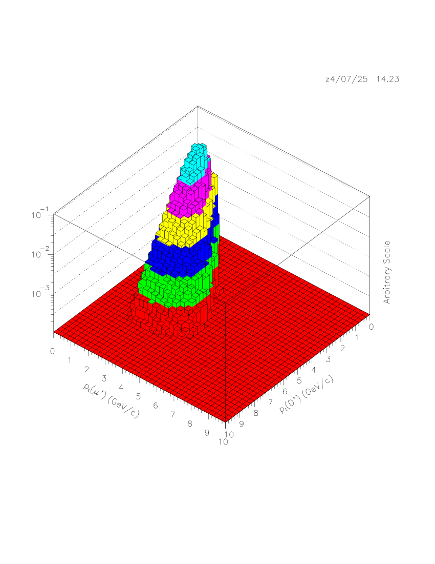
Figure 5.5 shows the projections of the histograms onto their respective axes to show the effect of applying a cross section (in this case an arbitrary $D$ cross section found during a minimization).

Figure 5.5: The $D$ spectrum of Figures 5.3 (top left) and 5.4 (top right) and the $\mu^{+}\;$spectra corresponding to the same Figures on bottom. All spectra are the projection of the 2-dimensional $p_{T}\left(\mu\right)\;$versus $p_{T}\left(h\right)\;$histograms onto their respective axes. Errors may be smaller than the symbols used, and include all systematic errors associated with the decay and branching fraction parameterizations used to calculate those weights as described in 5.4.

5.4 Errors Used For Calculating $\chi^{2}$

Only the statistical error was used for the data, $\varepsilon_{j}=\sqrt{s_{j}}$, where $s_{j}$ is the total number of muons in element $j$. Errors for Monte Carlo spectra included the systematic and statistical errors of the parameterizations used to calculate the primary weights $W_{x}$, $W_{A}$, $W_{D}$, $W_{NA}$ and $W_{br}$ for light hadrons and $W_{D}$, $W_{NA}$ and $W_{br}$ for the open charm hadrons. See table 4.1, page 4.1.

The total weight given an event in the Monte Carlo was defined as

$$W_{k}=W_{x,k}\,W_{A}\,W_{D}\,W_{NA}\,W_{br}$$

for light hadrons and

$$W_{k}=W_{D}\,W_{NA}\,W_{br}$$

for open charm hadrons. Hadrons thrown from the dump had $W_{NA}=1$. The statistical error of $s$ weighted events in a bin $j$ is determined from [42]:

$$\epsilon_{j}=\sqrt{\sum^{s}_{k=1}\left(W^{2}_{k}\right)}$$

.

All statistical or systematic errors of the parameterizations used in calculating the primary weights, $\sigma_{x}$, $\sigma_{A}$, $\sigma_{D}$, $\sigma_{NA}$ were also calculated. As an example, the systematic error, $\sigma_{x}$, of the differential cross section weight, $W_{x}$, of a light hadron was calculated as two parts, the errors of the parameters used to calculate the cross section, shown in Table 4.2 (page 4.2), plus the normalization uncertainty, both of which were taken from the reference. The error due to the uncertainties in the values of the parameters was calculated by use of the error propagation equation, excluding covariant terms

$$\sigma_{x,p}^{2}\simeq\sigma_{A_{1}}^{2}\left(\frac{\partial x}{\partial A_{1}}\right)^{2}+\sigma_{B}^{2}\left(\frac{\partial x}{\partial B}\right)^{2}+\cdots+\sigma_{m}^{2}\left(\frac{\partial x}{\partial m}\right)^{2}$$

where $x,p$ is used to show that the error is the error of the parameterization used for the light hadron differential cross section, $A_{1}$, $B$ and $m$ are three of those parameters and $\sigma_{A_{1}}$ is the error of the parameter $A_{1}$ taken from the reference. The second error associated with the light hadron differential cross section weight was the uncertainty in the absolute normalization, given by the reference as a relative error, $R_{x}$. The error due to the normalization uncertainty was calculated by $\sigma_{x,n}=W_{x}\,R_{x}$. The error associated with the light hadron cross section weight, $\sigma_{x}$ was then calculated as $\sigma^{2}_{x}=\sigma^{2}_{x,p}+\sigma^{2}_{x,n}$. Additional errors for all other weights were calculated using the error propagation equation and the errors of variables from the references. The error on $W_{br}$, $\sigma_{br}$ (strange and open charm hadrons only) was 0.2 percent (strange hadrons) and 11.5 percent (open charm hadrons) of the value of the branching fraction weight.

Each muon from the Monte Carlo contributed the square of its total weight as a statistical error, plus the square of the error of the weights for use in calculating the $\epsilon^{2}_{j}$

$$\epsilon^{2}_{j}=\sum^{s}_{k=1}\left[W^{2}_{k}+\sigma^{2}_{k}\right]$$

where $W_{k}$ is the total weight of muon $k$ and $\sigma^{2}_{k}$ is the square of the errors of the weights

$$\sigma^{2}_{k}=W^{2}_{k}\left[\frac{\sigma^{2}_{x,k}}{W^{2}_{x,k}}+\frac{\sigma^{2}_{A,k}}{W^{2}_{A,k}}+\frac{\sigma^{2}_{D,k}}{W^{2}_{D,k}}+\frac{\sigma^{2}_{NA.k}}{W^{2}_{NA,k}}+\frac{\sigma^{2}_{br,k}}{W^{2}_{br,k}}\right]$$

The squared error, $\epsilon^{2}_{j}$ for $s$ muons in a bin $j$ is then

$$\epsilon^{2}_{j}=\sum^{s}_{k=1}\left[W^{2}_{k}\,\left(1+\left\{\frac{\sigma^{2}_{x,k}}{W^{2}_{x,k}}+\frac{\sigma^{2}_{A,k}}{W^{2}_{A,k}}+\frac{\sigma^{2}_{D,k}}{W^{2}_{D,k}}+\frac{\sigma^{2}_{NA,k}}{W^{2}_{NA,k}}+\frac{\sigma^{2}_{br,k}}{W^{2}_{br,k}}\right\}\right)\right]$$ (5.6)

5.5 Parameter Errors

Error routines were developed based on MINUIT, the method used for error analysis of function minimizations used by CERN [43]. The errors of an $n$ dimensional function, including all correlations, can be determined using contours of equal likelihood. By choosing the appropriate amount to add to the value of $\chi^{2}_{min}$, referred to as UP, the errors on the $\chi^{2}_{min}\;$values of the parameters can be determined by minimization to $n-1$ dimensions of the original function, where one parameter is held fixed. In general, the method involves increasing or decreasing the value of the fixed parameter and then minimizing the remaining parameters until the smallest value of the total $\chi^{2}\;$returned (referred to as $\chi^{2}_{test}\;$here) remains smaller than or equal to $\chi^{2}_{max}$, where $\chi^{2}_{max}=\left(\chi^{2}_{min}+\mbox{{UP}}\right)$. The maximum and minimum values the free parameters had to take in order that $\chi^{2}_{test}\;$remain smaller than or equal to $\chi^{2}_{max}\;$during the entire process were returned as their errors.

The routines systematically increased/decreased the fixed parameters value by a pre-set amount until the returned value of $\chi^{2}_{test}\;$increased to more than $\chi^{2}_{max}$. Once this condition was met, the routine decreased the size of increment that the fixed parameter would increase/decrease and began minimization of the remaining free parameters where the value for the fixed parameter was the previous maximum or minimum value plus or minus the new increment size. This procedure was repeated until the increment size became smaller than $10^{-5}$. This experiment used values for UP for a 70% confidence level for both the $nv=3$ and $nv=4$ functions as given in Table 5.2.

Table 5.2: Values of UP for given confidence level and number of free parameters $n$. Taken from [43].

		Confidence level (probability contents desired
Number of		inside hypercontour of $\chi^{2}=\chi^{2}_{min}\;+\mbox{{UP}}$)
Parameters		50%	70%	90%	95%	99%
	1	0.46	1.07	2.70	3.84	6.63
	2	1.39	2.41	4.61	5.99	9.21
	3	2.37	3.67	6.25	7.82	11.36
	4	3.36	4.88	7.78	9.49	13.28
	5	4.35	6.06	9.24	11.07	15.09
	6	5.35	7.23	10.65	12.59	16.81
	7	6.35	8.38	12.02	14.07	18.49
	8	7.34	9.52	13.36	15.51	20.09
	9	8.34	10.66	14.68	16.92	21.67
	10	9.34	11.78	15.99	18.31	23.21
	11	10.34	12.88	17.29	19.68	24.71

5.6 Other Errors

This analysis did not require correcting the data for losses from acceptances, and the large error introduced by the addition of the two inside acceptance edges was minimized by cutting the first 5 data points from all spectra. Corrections for data lost due to data acquisition limitations, referred to as signal busy losses, are contained in the parameter $N$. Monte Carlo studies determined the uncertainty in the transverse momentum of the muons was less than 5 percent for the entire region above 2.0 GeV/c. This uncertainty has the effect of shifting the $p_{T}\;$spectrum to slightly higher values due to the fact that more events will ’feed down’ than will ’feed up’ because the spectrum is (approximately) exponentially decreasing as a function of $p_{T}$. The same effect is present in all Monte Carlo spectra as well, so the relative effect between the two is, for the most part, cancelled.

Loss of data due to inefficiencies in the hodoscopes was modeled in the Monte Carlo based on studies by the previous dimuon analysis. For that data all hodoscopes had efficiencies of over 96 percent, and for this analysis only the x measuring hodoscopes were needed. Similarly, loss from bad wires and noise in the wire planes was modeled in the Monte Carlo spectra based on studies from the same analysis. As a check, the data were plotted using the variable $\mbox{TAN}\theta_{x}$. This variable is very sensitive to the opening angle the muon trajectory had in the $x-z$ plane, and any significant loss of events from a defective hodoscope or phototube should be clearly discernable. No such defects in the spectra were found. (See Figure 3.11 page 3.11.)

Light hadrons have a small uncertainty at moderate to high transverse momentum associated with the parameterization used. The fits determined by the BSC are valid up to approximately 6 GeV/cin $p_{T}$[32]. The light hadron distributions above 6 GeV/c have an additional uncertainty estimated to be less than 10 percent. This uncertainty can be neglected since the light hadron contributions are less than 1 percent beyond 6 GeV/c (see figure 6.17).

Production of hadrons containing open bottom were ignored when calculating the total Monte Carlo spectra. Semi-leptonic decays of open bottom hadrons introduces a small contamination since the decay may give rise to both a $\mu^{+}\;$and a $\mu^{-}\;$(the semi-leptonic decay $B^{+}\rightarrow\mu^{+}\nu_{\mu}\overline{D}^{0}\;$ where the $\overline{D}^{0}\;$then decays semi-leptonically to a $\mu^{-}\;$is one example). The branching fractions of these modes are small, typically less than 3 percent, so contamination from production of open bottom is negligible.

Table 5.3 lists the estmated uncertainty of the fits due to the analyzed muon transverse momentum, hodoscope inefficiencies, light hadron normalization, choice of the transverse momentum of the open charm hadrons at the mid-point value of the bin and contamination of the spectra through semi-leptonic decay of open bottom production.

Table 5.3: Estimated errors on final cross sections from various sources not included in the errors of the parameters. The Muon and average hadron $p_{T}\;$are $p_{T}\;$dependent, and the error shown is the maximum for these errors at any $p_{T}$.

	Estimated
Source	Uncertainty (%)
Muon $p_{T}$	7
Average Hadron $p_{T}$	5
Hodoscopes	3
Light Hadron Normalization	$<$ 1
Contamination From Bottom	$<$ 1
Total	9.2

Chapter 6 Results

This analysis used single muon data to extract the open charm differential cross sections as a function of the hadron transverse momentum. Eight variations of three functions were fit to the data; an exponential, a three parameter polynomial with $n$ a free parameter, and both the three and four parameter polynomials with $n$ fixed at the integer values 4, 5 and 6 (see Chapter 5, page 5).

Table 6.1 gives the total number of muons in each data spectrum, the total number of muons in the data and the number of data points that each spectrum provided. Figure 6.1 shows the $p_{T}\left(\mu\right)\;$distributions from the copper target (top) and beryllium target (bottom). The vertical line represents the minimum transverse momentum used (2.25 GeV/c) during fitting.

Table 6.1: The number of muons, $N_{\mu}$, and the number of data points, $N_{DP}$, after final cuts were applied for all spectra used in this analysis. T indicates events from the targets, and D indicates events from the dump.

	Spectrum	$N_{\mu}$	$N_{DP}$
	$T^{+}$	16657	14
	$T{-}$	11954	14
	$D^{+}$	59576	20
Copper	$D{-}$	53322	18
Total		141689	66
	$T^{+}$	13368	16
	$T{-}$	9482	14
	$D^{+}$	120262	19
Beryllium	$D{-}$	109017	19
Total		252129	68

Figure 6.1: The single muon E866 data spectra. Top two figures are the $\mu^{+}\;$(red triangles) and $\mu^{-}\;$(blue upside down triangles) for the copper target data set from the target (left) and dump (right). Bottom row is the spectra from the beryllium target data set. Vertical lines show lower limit ($p_{T}\left(\mu\right)\geq 2.25GeV/c$) of the muon transverse-momentum used during fitting. Both dump figures are the events from the copper dump when the designated target (Cu or Be) was presented to the beam. Errors are statistical only.

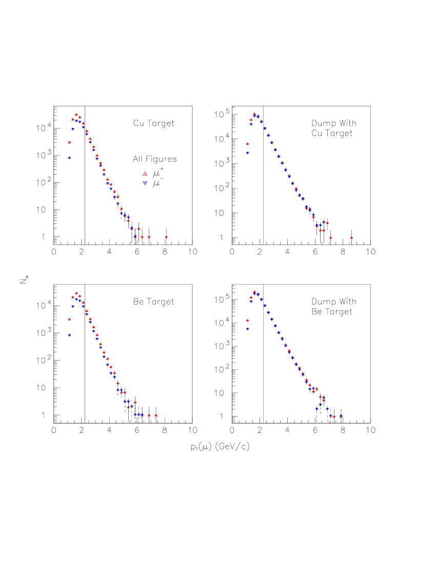
6.1 Fits To The Data

The values for the parameters for the best fits to the data using the exponential function are presented in Table 6.2, for the 3 parameter polynomial function in Table 6.3 and the four parameter polynomial in Tables 6.4 (copper) and 6.5 (beryllium). The total $\chi^{2}$, $\chi^{2}_{min}$, and reduced $\chi^{2}$, $\chi^{2}_{pdf}$, are also shown for the fit for each parameterization. From the tables, the author concludes:

• The 3 parameter function with either $n$ a free parameter or $n$ fixed at $n=6$ as well as the 4 parameter function with $n$ fixed at $n=6$ provided the best fits to the data.

• Though no errors were calculated for floating values of $n$, the weighted average value of $n$ for all fits with $n$ a free parameter was 6.18 $\pm$ 0.19.

• The exponential function provided a remarkably good fit for a large range in $p_{T}\left(h\right)\;$, $2.0\lesssim p_{T}\;\lesssim 7.0$ GeV/c.

• The 4 parameter function provides no additional information beyond that determined from fitting the 3 parameter function.

All fits of functions having 4 free parameters, the 3 parameter floating $n$ and all 4 parameter functions, had large correlations between the parameters. No errors were calculated for fits using the 3 parameter function with $n$ a free parameter. Because of the large correlations, two sets of errors were presented for fits using the fixed $n$ 4 parameter function; one where the parameter $\alpha$ was held constant at its $\chi^{2}_{min}\;$value (referred to as the fixed $\alpha$ errors), and one set where the parameter $m$ was held fixed at its $\chi^{2}_{min}\;$value (fixed $m$ errors).

Figures 6.2 through 6.9 show the total Monte Carlo spectra plotted against the data for four selected fits: the exponential function, the 3 parameter polynomial function with $n$ free and $n$ fixed to $n=6$, and the 4 parameter polynomial function with $n$ fixed to $n=6$. All Monte Carlo spectra are those at $\chi^{2}_{min}\;$for the function being fitted. Errors for the Monte Carlo spectra include all statistical plus all systematical errors as explained previously. The Monte Carlo errors do not include the errors for the parameters of the input open charm corss sections. All data spectra have statistical errors only. Figure 6.10 is the same as figure 6.6 except the open charm and light contributions are included.

Table 6.2: Parameter values from fits to the data using $A_{1}\,exp\left(-B\,p_{T}\right)\;$as the input shape of the open charm differential cross section. Values for $D$ are top line and $\overline{D}$ are the bottom line. Errors are the 70 percent confidence level errors as described in Chapter 5.5.

Copper Target Data
$A_{1}$		$B$		$N$		$\chi^{2}_{min}$	$\chi^{2}_{pdf}$
1.91	$+\,0.32\atop-\,0.27$	1.91	$+\,0.04\atop-\,0.04$
1.83	$+\,0.34\atop-\,0.28$	1.94	$+\,0.04\atop-\,0.04$	22.48	$0.23\atop 0.47$	81.4	1.3
Beryllium Target Data
$A_{1}$		$B$		$N$		$\chi^{2}_{min}$	$\chi^{2}_{pdf}$
0.60	$+\,0.14\atop-\,0.23$	2.11	$+\,0.06\atop-\,0.12$
0.57	$+\,0.16\atop-\,0.21$	2.18	$+\,0.07\atop-\,0.12$	42.11	$0.10\atop 0.66$	62.9	1.0

Table 6.3: Parameter values for $D$ (top line) and $\overline{D}$ (second line) from fits to the data where the differential cross section was input as $\frac{A_{2}}{\left(p_{T}^{2}+\alpha\,m_{c}^{2}\right)^{n}}$. Top two lines of both target data sets are the full float minimization. Errors are calculated for 70 percent confidence level as explained in Chapter 5.5.

Copper Target Data
$A_{2}$		$\alpha$		$n$	$N$		$\chi^{2}$	$\chi^{2}_{pdf}$
649710		4.14		6.32
286500		3.77		6.19	21.84		54.09	0.92
37.52	$+\,1.62\atop-\,3.45$	0.07	$+\,0.01\atop-\,0.07$		26.03	$+\,0.76\atop-\,0.68$
31.91	$+\,1.27\atop-\,2.81$	0.06	$+\,0.01\atop-\,0.06$	4.0	26.03	$+\,0.55\atop-\,0.55$	305.41	5.01
2334	$+\,217\atop-\,205$	1.71	$+\,0.12\atop-\,0.13$		22.39	$+\,0.17\atop-\,0.47$
1931	$+\,196\atop-\,181$	1.66	$+\,0.13\atop-\,0.14$	$5.0$	22.39	$+\,0.11\atop-\,0.35$	99.58	1.63
161765	$+\,19378\atop-\,15265$	3.53	$+\,0.17\atop-\,0.17$		21.70	$+\,0.11\atop-\,0.34$
130126	$+\,16808\atop-\,15265$	3.44	$+\,0.18\atop-\,0.19$	$6.0$	21.70	$+\,0.11\atop-\,0.23$	56.08	0.92
Beryllium Target Data
$A_{2}$		$\alpha$		$n$	$N$		$\chi^{2}_{min}$	$\chi^{2}_{pdf}$
19238		3.03		6.06
17013		2.92		6.14	42.19		60.14	0.99
6.50	$+\,0.34\atop-\,0.83$	0.08	$+\,0.01\atop-\,0.08$		42.39	$+\,0.67\atop-\,0.67$
4.88	$+\,0.25\atop-\,0.65$	0.08	$+\,0.01\atop-\,0.08$	$4.0$	42.39	$+\,0.66\atop-\,0.67$	167.32	2.66
289	$+\,29\atop-\,75$	1.46	$+\,0.13\atop-\,0.39$		41.97	$+\,0.20\atop-\,0.46$
225	$+\,13\atop-\,100$	1.50	$+\,0.08\atop-\,0.73$	$5.0$	41.97	$+\,0.24\atop-\,0.92$	84.44	1.34
15280	$+\,3847\atop-\,3046$	2.94	$+\,0.32\atop-\,0.30$		42.13	$+\,0.11\atop-\,0.44$
11280	$+\,1546\atop-\,4055$	2.91	$+\,0.18\atop-\,0.58$	$6.0$	42.13	$+\,0.11\atop-\,0.67$	62.19	0.99

Table 6.4: The $\chi^{2}_{min}\;$parameter values when the open charm differential cross section was input in the form $A_{2}\,\frac{\left(1-p_{T}\,/\,p_{beam}\right)^{m}}{\left(p_{T}^{2}+\alpha\,m_{c}^{2}\right)^{n}}$and fitted to the copper target data. Top line is for $D$ and second line is for $\overline{D}$. All fits had $n$ fixed to the values shown. $p_{beam}=19.38$ GeV/c for this analysis. Errors were calculated holding $\alpha$ fixed at its $\chi^{2}_{min}\;$value (top pair of lines for each $n$) and holding $m$ fixed at its $\chi^{2}_{min}\;$value (bottom pair of lines for each $n$) because of strong correlations. Errors are calculated for 70 percent confidence level as explained in Chapter 5.5.

Copper Target Data
$A_{2}$		$\alpha$		$n$	$m$		$N$		$\chi^{2}_{min}$	$\chi^{2}_{pdf}$
1412	$+\,180\atop-\,171$	2.75			8.00	$+\,0.47\atop-\,0.48$		$+\,0.22\atop-\,0.33$
1616	$+\,217\atop-\,220$	2.99			8.80	$+\,0.51\atop-\,0.57$		$+\,0.11\atop-\,0.33$
1412	$+\,158\atop-\,156$	2.75	$+\,0.22\atop-\,0.24$		8.00			$+\,0.16\atop-\,0.23$
1616	$+\,196\atop-\,206$	2.99	$+\,0.25\atop-\,0.29$	$4.0$	8.80		21.02	$+\,0.10\atop-\,0.22$	58.48	0.99
15959	$+\,2120\atop-\,1774$	3.30			4.17	$+\,0.47\atop-\,0.44$		$+\,0.22\atop-\,0.46$
10804	$+\,1520\atop-\,1283$	3.02			3.81	$+\,0.51\atop-\,0.51$		$+\,0.10\atop-\,0.24$
15959	$+\,1940\atop-\,1740$	3.30	$+\,0.20\atop-\,0.21$		4.17			$+\,0.12\atop-\,0.35$
10804	$+\,1371\atop-\,1243$	3.02	$+\,0.21\atop-\,0.21$	$5.0$	3.81		21.95	$+\,0.12\atop-\,0.23$	54.61	0.93
300220	$+\,39248\atop-\,33390$	4.07			1.29	$+\,0.46\atop-\,0.43$		$+\,0.20\atop-\,0.36$
137891	$+\,19998\atop-\,8836$	3.48			0.13	$+\,0.52\atop-\,0.13$		$+\,0.34\atop-\,0.24$
300220	$+\,39002\atop-\,34736$	4.07	$+\,0.20\atop-\,0.20$		1.29			$+\,0.11\atop-\,0.34$
137891	$+\,18010\atop-\,16242$	3.48	$+\,0.19\atop-\,0.19$	$6.0$	0.13		21.75	$+\,0.11\atop-\,0.23$	54.23	0.92

Table 6.5: The $\chi^{2}_{min}\;$parameter values when the open charm differential cross section was input in the form $A_{2}\,\frac{\left(1-p_{T}\,/\,p_{beam}\right)^{m}}{\left(p_{T}^{2}+\alpha\,m_{c}^{2}\right)^{n}}$and fitted to the beryllium target data. Top line is for $D$ and second line is for $\overline{D}$. All fits had $n$ fixed to the values shown. $p_{beam}=19.38$ GeV/c for this analysis. Errors were calculated holding $\alpha$ fixed at its $\chi^{2}_{min}\;$value (top pair of lines for each $n$) and holding $m$ fixed at its $\chi^{2}_{min}\;$value (bottom pair of lines for each $n$) because of strong correlations. Errors are calculated for 70 percent confidence level as explained in Chapter 5.5.

Beryllium Target Data
$A_{2}$		$\alpha$		$n$	$m$		$N$		$\chi^{2}_{min}$	$\chi^{2}_{pdf}$
508	$+\,153\atop-\,117$	3.34			11.23	$+\,1.17\atop-\,1.15$		$+\,0.10\atop-\,0.67$
402	$+\,136\atop-\,97$	3.15			11.87	$+\,1.33\atop-\,1.24$		$+\,0.11\atop-\,0.44$
508	$+\,142\atop-\,119$	3.34	$+\,0.57\atop-\,0.57$		11.23			$+\,0.07\atop-\,0.44$
402	$+\,126\atop-\,100$	3.15	$+\,0.60\atop-\,0.58$	$4.0$	11.87		42.18	$+\,0.04\atop-\,0.44$	59.30	0.97
4151	$+\,1228\atop-\,903$	3.46			6.50	$+\,1.15\atop-\,1.06$		$+\,0.10\atop-\,0.45$
3483	$+\,1157\atop-\,810$	3.37			7.25	$+\,1.30\atop-\,1.18$		$+\,0.10\atop-\,0.44$
4151	$+\,1167\atop-\,946$	3.46	$+\,0.46\atop-\,0.45$		6.50			$+\,0.11\atop-\,0.45$
3483	$+\,1105\atop-\,860$	3.37	$+\,0.50\atop-\,0.47$	$5.0$	7.25		42.18	$+\,0.05\atop-\,0.44$	58.44	0.96
67537	$+\,19855\atop-\,14577$	4.11			3.31	$+\,1.13\atop-\,1.05$		$+\,0.19\atop-\,0.45$
68581	$+\,22785\atop-\,16101$	4.19			4.49	$+\,1.32\atop-\,1.20$		$+\,0.21\atop-\,0.45$
67537	$+\,20187\atop-\,16248$	4.11	$+\,0.43\atop-\,0.43$		3.31			$+\,0.10\atop-\,0.67$
68581	$+\,23679\atop-\,18335$	4.19	$+\,0.49\atop-\,0.48$	$6.0$	4.49		42.18	$+\,0.05\atop-\,0.44$	58.25	0.95

Figure 6.2: The copper target data (black closed circles) and total Monte Carlo spectra at $\chi^{2}_{min}\;$(red open circles) from the fit where the $D/\overline{D}$ cross sections were of the form $A_{1}\,exp\left(-B\,p_{T}\right)$. Histograms are $\mu^{+}\;$(left) and $\mu^{-}\;$(right) for the copper target (top) and copper dump (bottom). Errors for the data are statistical only. Errors for the Monte Carlo include all errors used for calculating $\chi^{2}$(see text). Error bars may be smaller than symbols used.

Figure 6.3: The beryllium target data (black closed circles) and total Monte Carlo spectra at $\chi^{2}_{min}\;$(red open circles) from the fit where the $D/\overline{D}$ cross sections were of the form $A_{1}\,exp\left(-B\,p_{T}\right)$. Histograms are $\mu^{+}\;$(left) and $\mu^{-}\;$(right) for the beryllium target (top) and copper dump (bottom). Errors for the data are statistical only. Errors for the Monte Carlo include all errors used for calculating $\chi^{2}$(see text). Error bars may be smaller than symbols used.

Figure 6.4: The copper target data (black closed circles) and total Monte Carlo spectra at $\chi^{2}_{min}\;$(red open circles) from the fit where the $D/\overline{D}$ cross sections were of the form $\frac{A_{2}}{\left(p_{T}^{2}+\alpha\,m_{c}^{2}\right)^{n}}$. The exponent $n$ was a free parameter for this fit. Histograms are $\mu^{+}\;$(left) and $\mu^{-}\;$(right) for the copper target (top) and copper dump (bottom). Errors for the data are statistical only. Errors for the Monte Carlo include all errors used for calculating $\chi^{2}$(see text). Error bars may be smaller than symbols used.

Figure 6.5: The beryllium target data (black closed circles) and total Monte Carlo spectra at $\chi^{2}_{min}\;$(red open circles) from the fit where the $D/\overline{D}$ cross sections were of the form $\frac{A_{2}}{\left(p_{T}^{2}+\alpha\,m_{c}^{2}\right)^{n}}$. The exponent $n$ was a free parameter for this fit. Histograms are $\mu^{+}\;$(left) and $\mu^{-}\;$(right) for the beryllium target (top) and copper dump (bottom). Errors for the data are statistical only. Errors for the Monte Carlo include all errors used for calculating $\chi^{2}$(see text). Error bars may be smaller than symbols used.

Figure 6.6: The copper target data (black closed circles) and total Monte Carlo spectra at $\chi^{2}_{min}\;$(red open circles) from the fit where the $D/\overline{D}$ cross sections were of the form $\frac{A_{2}}{\left(p_{T}^{2}+\alpha\,m_{c}^{2}\right)^{n}}$. The exponent $n$ was fixed at $n=6$ for this fit. Histograms are $\mu^{+}\;$(left) and $\mu^{-}\;$(right) for the copper target (top) and copper dump (bottom). Errors for the data are statistical only. Errors for the Monte Carlo include all errors used for calculating $\chi^{2}$(see text). Error bars may be smaller than symbols used.

Figure 6.7: The beryllium target data (black closed circles) and total Monte Carlo spectra at $\chi^{2}_{min}\;$(red open circles) from the fit where the $D/\overline{D}$ cross sections were of the form $\frac{A_{2}}{\left(p_{T}^{2}+\alpha\,m_{c}^{2}\right)^{n}}$. The exponent $n$ was fixed at $n=6$ for this fit. Histograms are $\mu^{+}\;$(left) and $\mu^{-}\;$(right) for the beryllium target (top) and copper dump (bottom). Errors for the data are statistical only. Errors for the Monte Carlo include all errors used for calculating $\chi^{2}$(see text). Error bars may be smaller than symbols used.

Figure 6.8: The copper target data (black closed circles) and total Monte Carlo spectra at $\chi^{2}_{min}\;$(red open circles) from the fit where the $D/\overline{D}$ cross sections were of the form $A_{2}\,\frac{\left(1-p_{T}\,/\,p_{beam}\right)^{m}}{\left(p_{T}^{2}+\alpha\,m_{c}^{2}\right)^{n}}$. The exponent $n$ was fixed at $n=6$ for this fit. Histograms are $\mu^{+}\;$(left) and $\mu^{-}\;$(right) for the copper target (top) and copper dump (bottom). Errors for the data are statistical only. Errors for the Monte Carlo include all errors used for calculating $\chi^{2}$(see text). Error bars may be smaller than symbols used.

Figure 6.9: The beryllium target data (black closed circles) and total Monte Carlo spectra at $\chi^{2}_{min}\;$(red open circles) from the fit where the $D/\overline{D}$ cross sections were of the form $A_{2}\,\frac{\left(1-p_{T}\,/\,p_{beam}\right)^{m}}{\left(p_{T}^{2}+\alpha\,m_{c}^{2}\right)^{n}}$. The exponent $n$ was fixed at $n=6$ for this fit. Histograms are $\mu^{+}\;$(left) and $\mu^{-}\;$(right) for the beryllium target (top) and copper dump (bottom). Errors for the data are statistical only. Errors for the Monte Carlo include all errors used for calculating $\chi^{2}$(see text). Error bars may be smaller than symbols used.

Figure 6.10: The copper target data (black closed circles) and total Monte Carlo spectra at $\chi^{2}_{min}\;$(red open circles) from the fit where the $D/\overline{D}$ cross sections were of the form $\frac{A_{2}}{\left(p_{T}^{2}+\alpha\,m_{c}^{2}\right)^{n}}$. Blue triangles are the open charm contribution and the green upside-down triagles are the contribution from light hadrons. The exponent $n$ was fixed at $n=6$ for this fit. Histograms are $\mu^{+}\;$(left) and $\mu^{-}\;$(right) for the copper target (top) and copper dump (bottom). Errors for the data are statistical only. Errors for the Monte Carlo include all errors used for calculating $\chi^{2}$(see text). Contributions contain all systematic errors used in calculation of the weights added in quadrature to the statistical error, but do not include errors of the fit. Error bars may be smaller than symbols used.

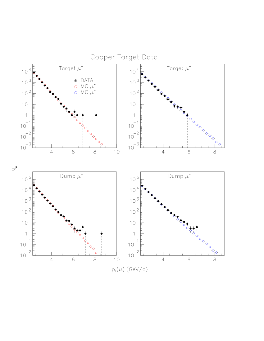
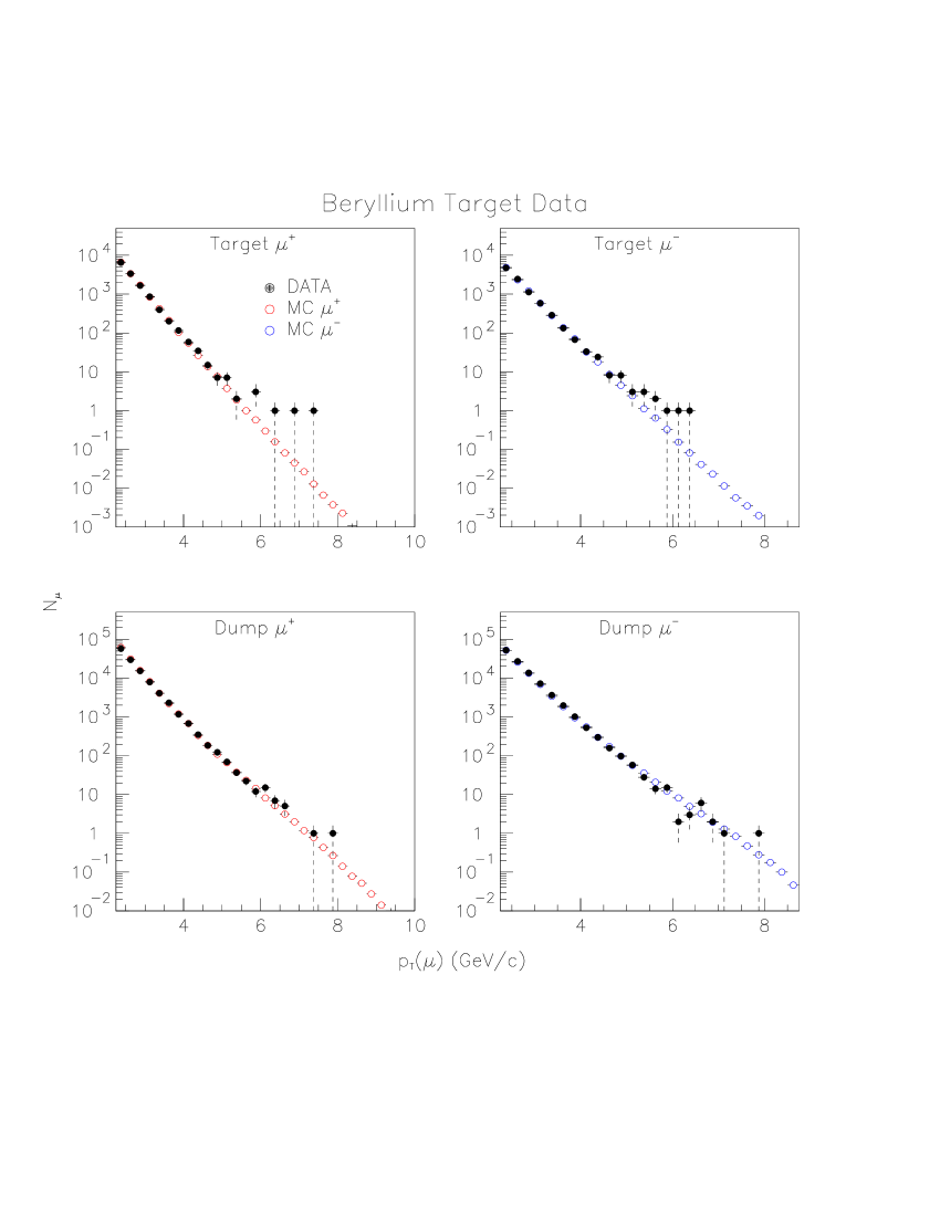
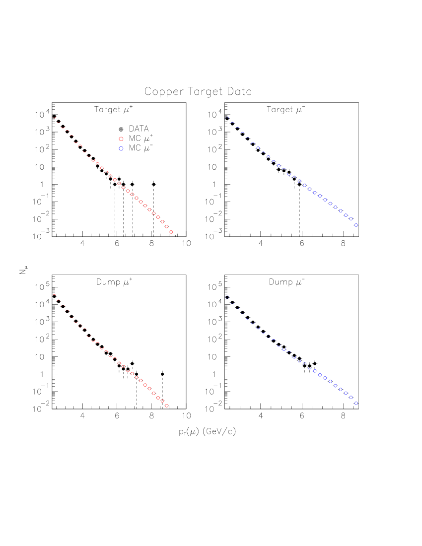
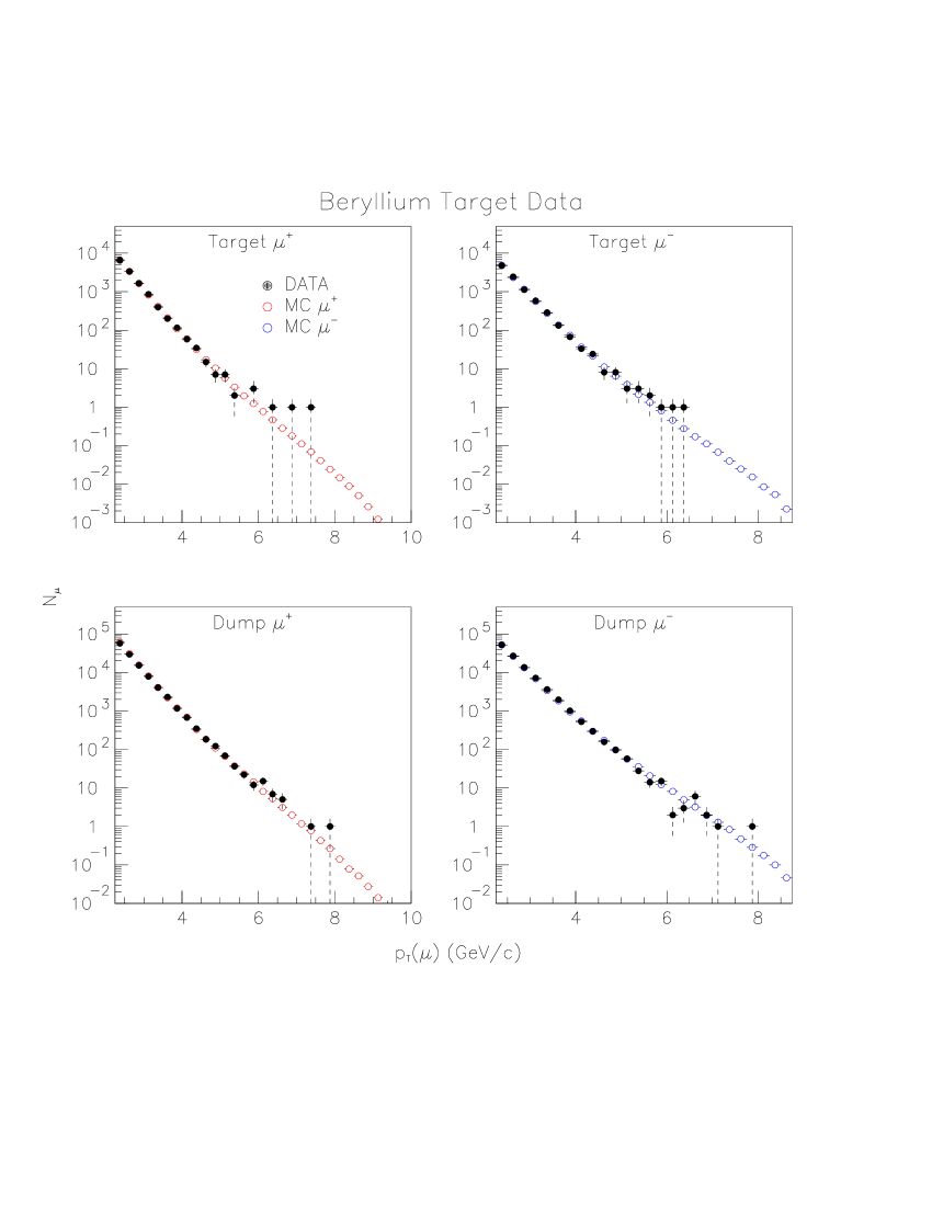
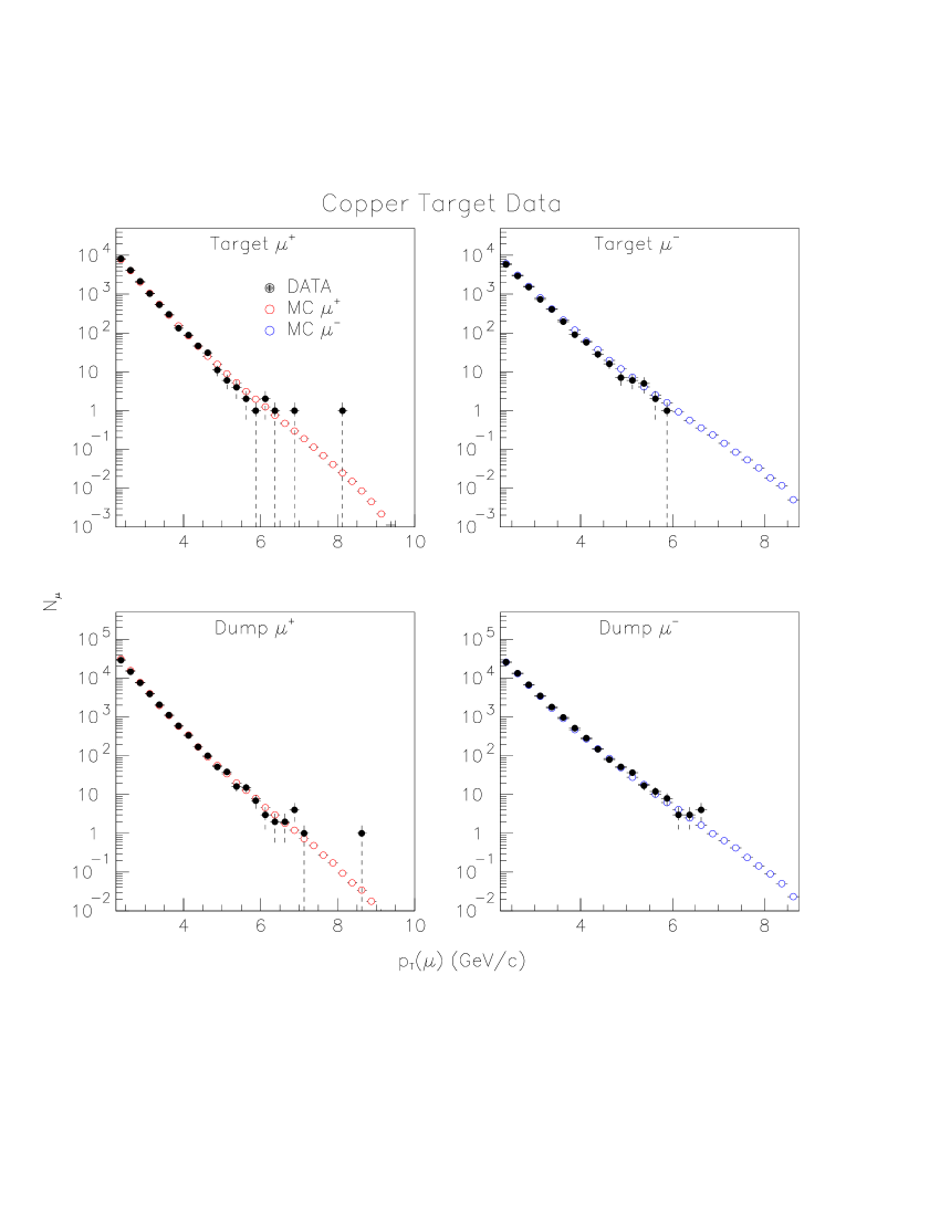
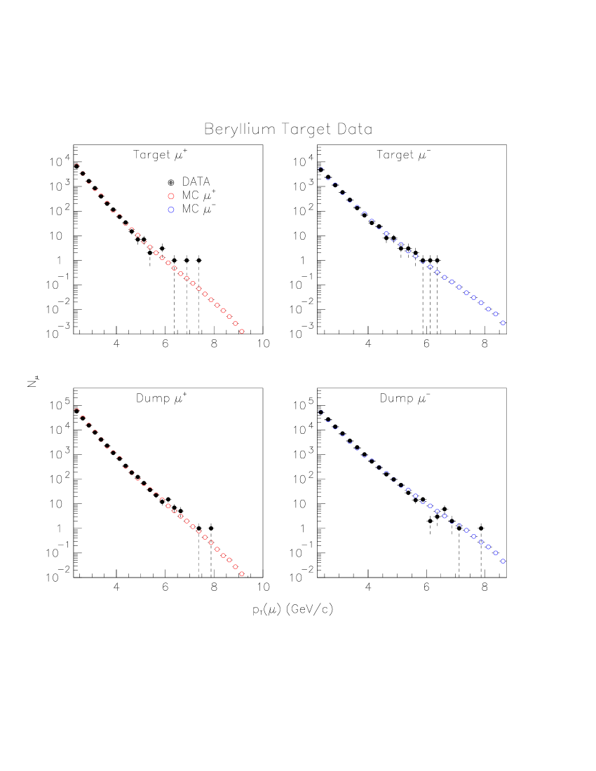
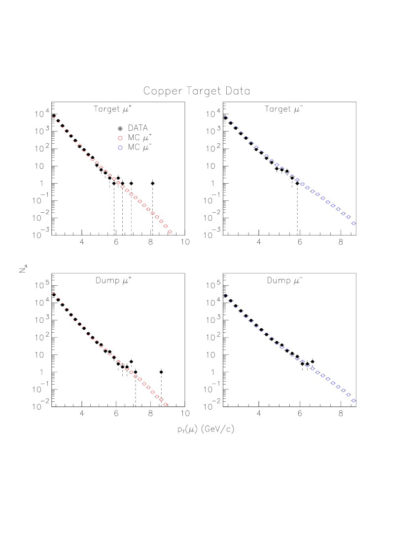
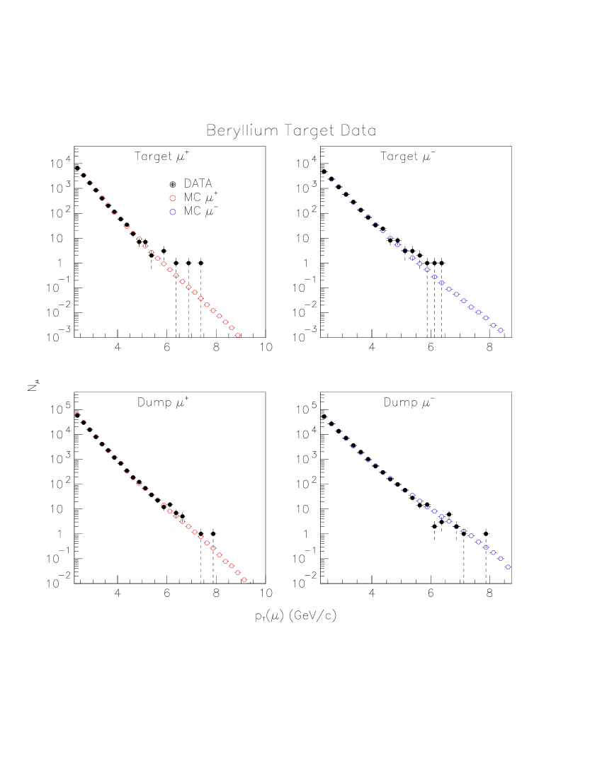
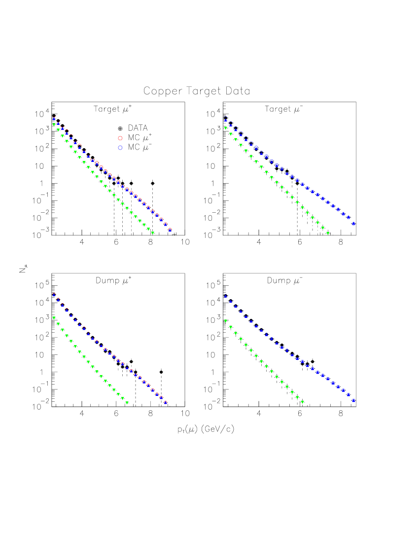
6.2 The Open Charm And Anti-charm Cross Sections

The differential p-Cu  and p-Be  open charm cross sections, determined from fits to the data shown in figures 6.2 through 6.9 are shown in figures 6.11 and 6.12. Errors were calculated using the error propagation equation as described in 5.4 for the parameters in the function used to describe the cross section added in quadrature to the error of the scaling variable $N$. The error shown represents a 70 percent confidence level that if the value of the first parameter was held within the stated range in values, the cross section would lie between the upper and lower error bars. Errors for the 4 parameter function were performed twice because of large correlations; one set of errors were calculated holding the value of $\alpha$ fixed (solid lines), and one set with $m$ fixed (dashed lines). Fits to the 3 parameter function with $n$ a free parameter had large correlations as well, and no errors were calculated for those fits. For clarity, the same cross sections are plotted without errors in figure 6.13. The p-Cu  and p-Be  $D$ and $\overline{D}$ differential cross sections are plotted together for the four selected functions in figures 6.14, and 6.15. The four fits selected appear to be well constrained, even when projected to $p_{T}=0$ GeV/c, as shown in figure 6.16. Figure 6.17 shows the $D$ differential cross section scaled by $A=63.546$ plotted with the $\pi^{+}\;$and $K^{+}\;$cross sections given in [32].

Figure 6.11: The differential cross sections for $D$ (left) and $\overline{D}$ (right) determined from fits to the copper data for the various functions: exponential (black), 3 parameter with $n$ a free parameter (red), the 3 parameter with $n$ fixed to $n=6$ (blue) and the 4 parameter with $n=6$ (green). Errors shown include the error on $N$ added in quadrature.

Figure 6.12: The differential cross sections for $D$ (left) and $\overline{D}$ (right) determined from fits to the beryllium data for the various function: exponential (black), 3 parameter with $n$ a free parameter (red), the 3 parameter with $n$ fixed to $n=6$ (blue) and the 4 parameter with $n=6$ (green). Errors shown include the error on $N$ added in quadrature.

Figure 6.13: The p-Cu  (top) and p-Be  (bottom) $D$ (left) and $\overline{D}$ (right) differential cross sections from fits to the data for the various functions: exponential (black), 3 parameter with $n$ a free parameter (red), 3 parameter with $n=6$ (blue) and the 4 parameter with $n=6$ (green). No errors are shown for clarity.

Figure 6.14: The p-Cu  $D$ (black) and $\overline{D}$ (red) differential cross sections for the various functions: exponential (top left), 3 parameter with $n$ a free parameter (top right), 3 parameter with $n$ fixed at $n=6$ (bottom left) and the 4 parameter function with $n$ fixed at $n=6$. Errors include the error on the parameter $N$ added in quadrature.

Figure 6.15: The p-Be  $D$ (black) and $\overline{D}$ (red) differential cross sections for the various functions: exponential (top left), 3 parameter with $n$ a free parameter (top right), 3 parameter with $n$ fixed at $n=6$ (bottom left) and the 4 parameter function with $n$ fixed at $n=6$. Errors include the error on the parameter $N$ added in quadrature.

Figure 6.16: The p-Cu  $D$ differential cross section projected to low $p_{T}\;$for the various functions: exponential (black), 3 parameter with $n$ a free parameter (red), 3 parameter with $n$ fixed at $n=6$ (blue) and the 4 parameter function with $n$ fixed at $n=6$ (green). No errors are shown.

Figure 6.17: The p-Cu  $D$ differential cross section projected to low $p_{T}\;$for the 3 parameter function with $n=6$, and scaled down by $A=63.546$ (blue). Black is the $\pi^{+}\;$and red is the $K^{+}\;$differential p-p  cross sections as given in [32].

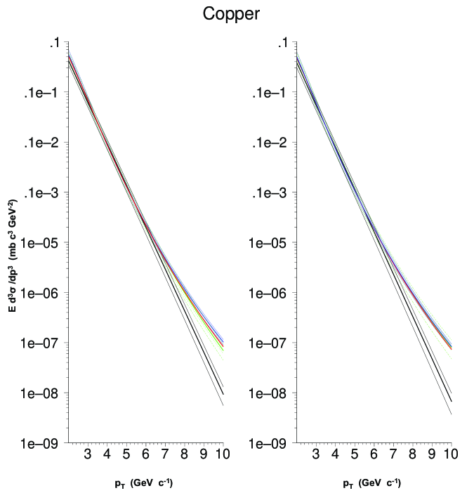
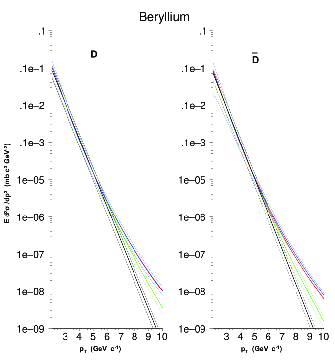
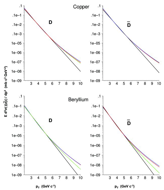
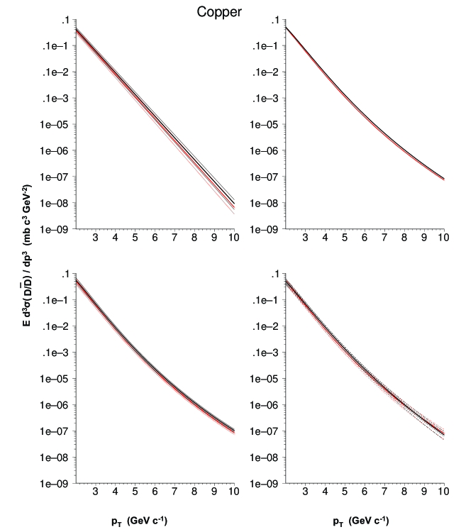
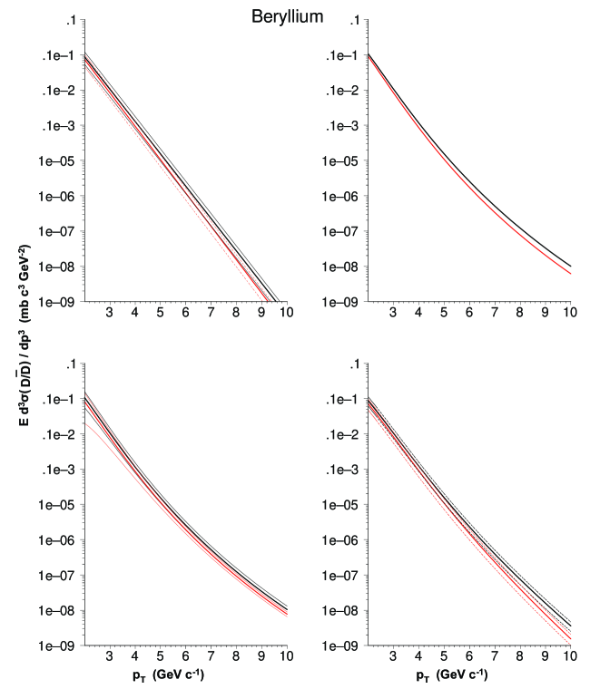
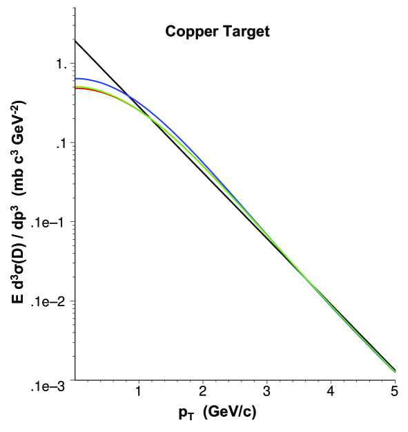
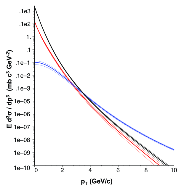
6.2.1 Comparison To Other Experiments

The open charm cross sections from this analysis were extracted from single muon events from 2.25 to $\sim$7 GeV/c. Extensive Monte Carlo studies have determined that contributions from open charm hadrons to the single muon spectra had $0.2\lesssim x_{F}\lesssim 0.8$ and $2.25\lesssim p_{T}\lesssim 7.0$ (GeV/c). The open charm cross sections were extracted using 3 functions to describe the shape of the cross section: $A_{1}\,exp\left(-B\,p_{T}\right)$, $\frac{A_{2}}{\left(p_{T}^{2}+\alpha\,m_{c}^{2}\right)^{n}}$and $A_{2}\,\frac{\left(1-p_{T}\,/\,p_{beam}\right)^{m}}{\left(p_{T}^{2}+\alpha\,m_{c}^{2}\right)^{n}}$. Comparison to other p-p  or p-A  results at similar energies is problematical since all fit their data to functions dissimilar to those chosen here. The increased range in transverse-momentum from this analysis is far beyond other p-A  experiments at this energy, covering a much larger range in $x_{F}$ as well.

The LEBC-MPS Collaboration (E743) [6] fitted their 800 GeV/c p-p  data with the function

$$\left(1-|\,x_{F}\,|\right)^{n}e^{-a\,p_{T}^{2}}$$

and E789 [8] fitted their results from 800 GeV/c p-A  data with the function

$$p_{T}\,e^{-n\,p_{T}^{2}}$$

The exponential using the square of the transverse-momentum failed to adequately describe the data from this analysis because it falls too steeply over the range in transverse-momentum.

Figure 1.5 shows the per nucleon total inclusive neutral open charm cross section from E789, and Figure 1.4 shows the p-p  total inclusive open charm cross section from E743. For comparison to the results from this analysis, the E743 data was divided by 2 since their results were the total open charm cross section which is assumed to be twice the neutral cross sections determined by E789 and twice the sum of the $D$ and $\overline{D}$ cross sections found by this analysis, and both the E743 and E789 results were scaled by $A_{Cu}=63.546$ and $A_{Be}=9.012182$. The sum of the $D$ and $\overline{D}$ cross sections determined from fitting the 3 parameter function with $n=6$ to the p-Cu  data is plotted with the scaled results from E743 (left) and E789 (right) in Figure 6.18, and the result from fitting the same function to the p-Be  data is shown in Figure 6.19. The reader is cautioned that the cross sections shown from this analysis below 2.25 GeV/c are the projected cross sections, since the analysis used no data below that momentum. The reader is also cautioned that both the E743 and E789 data are scaled to $A$ assuming $\alpha(p_{T})=1.0$ (this is a result presented in E789). These comparisons have also ignored the ratio of charged to neutral production. These figures show the results from this analysis lie between the two previous measurements. This confirms that the use of single muon spectra and the methods adopted by this analysis to extract the differential cross sections provided reasonable results.

Table 6.6 provides results from selected experiments. It lists the type of data, $p_{T}\;$and $x_{F}$ ranges covered, the function(s) and values of the parameters from fits to their data and results from this analysis. From figures 6.18, 6.19 and the table the author concludes:

• The open charm cross sections from this analysis reproduce the open charm $p_{T}\;$distributions from both previous 800 GeV/c p-p  and p-A  experiments, when projected to low hadron $p_{T}$.

• Data from 250 GeV/c p-A  interactions (E769 [9]) was fit to the exponential function. The value of $B$ reported was 3.0 $\pm$ 0.3, while the value of $B$ found by this analysis was 1.91 $\pm$ 0.04 (copper) and 2.11 $\pm$ 0.12 (beryllium). This is reasonable since the E769 data was from $0.0\leq p_{T}\;\leq\sqrt{10}$ GeV/c, while the data from this analysis is at higher $p_{T}$. The slope of the cross section becomes smaller with increasing $p_{T}\;$, as evidenced by the results from this experiment.

• 250 GeV/c $\pi$-A data from E769 was fitted with the 3 parameter function, where $\alpha=1.4\pm 0.3$ and $n=5.0\pm 0.6$. This analysis determined that $n=6$ and $\alpha\sim 3.5$ (copper) and $\alpha\sim 2.9$ (beryllium), indicating that open charm production, as a function of $p_{T}$, is softer for proton interactions than meson interactions (see figure 1.6).

Table 6.6: Top is the experiment, interaction, beam momentum and range in $p_{T}\;$and $x_{F}$ covered. Bottom table gives the parameterizations used to fit the data by the experiment and the values of the parameters reported. Note that the value of $B^{\prime}$ from E789 does not include all $p_{T}\;$dependencies of the function used by that experiment (see text). Values given for this analysis (E866) are for fits to determine the $D$ cross section only. N/A indicates that the parameterization was attempted but resulted in very large $\chi^{2}_{min}\;$and the values of the parameters are not shown. Comparison of the cross sections from this analysis and the E743 and E789 experiments are shown in figures 6.18 and 6.19.

Experiment And Data
		$p_{b}$	$p_{T}$
		GeV/c	GeV/c	$x_{F}$
	$\pi^{\pm}$-A	250	0 - 4	-0.1 - 0.8
E769 [9]	p-A	250	0 - $\sqrt{10}$	-0.1 - 0.5
E743 [6]	p-p	800	0 - $\sqrt{5}$	-0.1 - 0.4
E789 [8]	p-A	800	0 - 1.1	0.00 - 0.08
	p-Cu
E866	p-Be	800	2.25 $\sim$ 7.0	0.2 - 0.8
Parameterizations And Values
	$e^{-B^{\prime}\,p_{T}^{2}}$	$e^{-B\,p_{T}}$	$\left(p_{T}^{2}+\alpha\,m^{2}_{c}\right)^{-n}$
	$B^{\prime}$	$B$	$\alpha$	$n$
	1.08 $\pm$ 0.05	2.74 $\pm$ 0.09	1.4 $\pm$ 0.3	5.0 $\pm$ 0.6
E769	1.08 $\pm$ 0.05	3.0 $\pm$ 0.3
E743	0.8 $\pm$ 0.2
E789	0.91 $\pm$ 0.12
		1.91 $+\,0.04\atop-\,0.04$	3.53 $+\,0.17\atop-\,0.17$	6
E866	N/A	2.11 $+\,0.06\atop-\,0.12$	2.94 $+\,0.32\atop-\,0.30$	6

Figure 6.18: Comparison of the results from this analysis from fitting the p-Cu  data using the 3 parameter function with $n=6$ to the E743[6] (left) and E789[8] (right) data. The cross section from this analysis is the sum of the $D$ and $\overline{D}$ cross sections. The invariant cross sections for E743 and E789 were determined by dividing their published results by $\int^{1}_{-1}\,\left(1-|x_{F}|\right)^{8.6}\times 2\times\pi$. The data were then scaled by $A_{Cu}=63.546$. Black vertical line indicates the minimium $p_{T}\left(\mu\right)\;$data used by this analysis. The reader is cautioned that the data from E743 and E789 are evaluated at $x_{F}=y=0$ and compared to the cross section from this analysis projected to lower momentum.

Figure 6.19: Comparison of the results from this analysis from fitting the p-Be  data using the 3 parameter function with $n=6$ to the E743[6] (left) and E789[8] (right) data. The cross section from this analysis is the sum of the $D$ and $\overline{D}$ cross sections. The invariant cross sections for E743 and E789 were determined by dividing their published results by $\int^{1}_{-1}\,\left(1-|x_{F}|\right)^{8.6}\times 2\times\pi$. The data were then scaled by $A_{Be}=9.012182$. Black vertical line indicates the minimium $p_{T}\left(\mu\right)\;$data used by this analysis. The reader is cautioned that the data from E743 and E789 are evaluated at $x_{F}=y=0$ and compared to the cross section from this analysis projected to lower momentum.

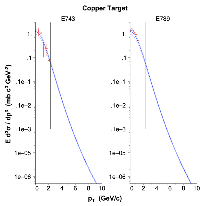
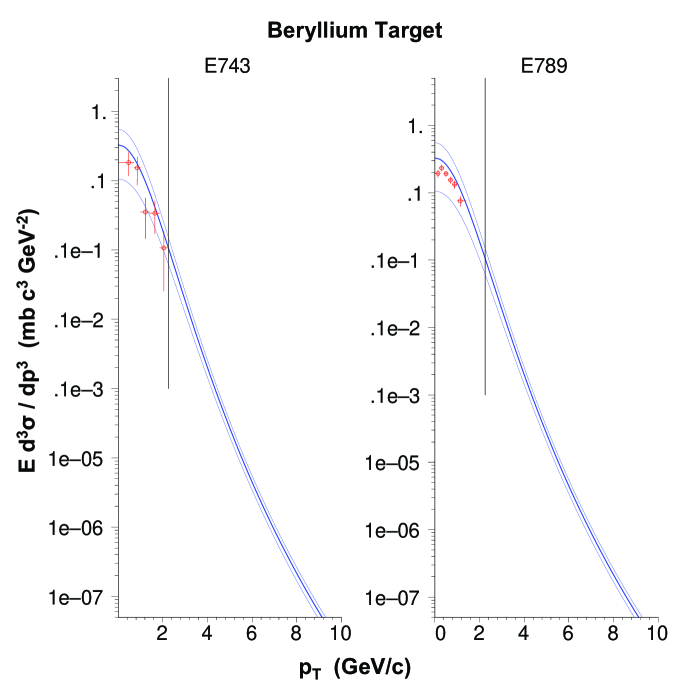
6.2.2 The Ratio Of Charged To Neutral Production

Theory suggests that

$$R_{CN}=\frac{\sigma\left(D^{+}\right)}{\sigma\left(D^{0}\right)}\sim 0.32$$

where $R_{CN}$ is the ratio of charged to neutral open charm production [5] [12]. Prior to 2000, experimental results from proton induced charm production showed the ratio to be consistent with unity [6] [7]. Results from the production of open charm via pion-nucleon interactions show the ratio from 0.27 to 0.50. The discrepancy between the ratios from meson interactions versus proton interactions, which should be the same, has generated some interest in the community [5]. A more recent study by the HERA-B collaboration [13] found the ratio to be 0.54 $\pm$ 0.11 $\pm$ 0.14 in 920 GeV/c p-A  collisions. Table 6.7 shows four experimentally determined charged to neutral production ratios for open charm from p-p  and p-A  interactions.

Table 6.7: The charged to neutral production ratio, $R_{CN}$, from other p-p  or p-A  experiments.

		Momentum
Experiment		GeV/c	Ratio
E783 [6]	p-p	800	1.2 $\pm$ 0.6
E653 [7]	p-A	800	1.0 $\pm$ 0.6
LEBC-EHS [48]	p-p	400	0.7 $\pm$ 0.1
HERA-B [13]	p-A	920	0.54 $\pm$ 0.18
Weighted Average			0.7 $\pm$ 0.1

This analysis lacks the sensitivity required to measure the charged to neutral production ratio, $R_{CN}$. This is due to the large transverse momentum shift from the parent hadron to the decay muon. This shift resulted in the shapes of the muon spectra being very similar for all open charm hadrons. During fitting the contributions from both the charged and neutral open charm mesons were added together, to give the total open charm Monte Carlo contribution. The analysis used $R_{CN}=1$ for all fits, so the two open charm cross sections determined from each fit were designated as $E\,\frac{d^{3}\,\sigma\left(D\right)}{d\,p^{3}}\left(p_{T}\right)\;$and $E\,\frac{d^{3}\,\sigma\left(\overline{D}\right)}{d\,p^{3}}\left(p_{T}\right)$. The $D$ cross section was then the cross section for either $D^{+}\;$or $D^{0}$, and the $\overline{D}$ cross section was the cross section for either the $D^{-}\;$or $\overline{D}^{0}$.

By using a charged to neutral production ratio other than 1, fitting would then be to either the charged cross section, or the neutral cross section, depending on how the ratio was introduced into calculating the open charm and open anti-charm Monte Carlo spectra. An open charm Monte Carlo spectrum is used as an example. The open charm contribution was determined from

$$W^{\mu}_{j}=\sum_{i=1}^{40}\left[\left(W^{\sigma_{D}}_{x,i}\,\mathbf{W}^{D^{+}\rightarrow\mu^{+}}_{i\,j}\right)+\left(W^{\sigma_{D}}_{x,i}\,\mathbf{W}^{D^{0}\rightarrow\mu^{+}}_{i\,j}\right)\right]$$

Choosing $\sigma_{D^{+}}=R\,\sigma_{D^{0}}$ the equation above may be re-written as

$$W^{\mu}_{j}=\sum_{i=1}^{40}\left[\left(R\,W^{\sigma_{D^{0}}}_{x,i}\,\mathbf{W}^{D^{+}\rightarrow\mu^{+}}_{i\,j}\right)+\left(W^{\sigma_{D^{0}}}_{x,i}\,\mathbf{W}^{D^{0}\rightarrow\mu^{+}}_{i\,j}\right)\right]$$

Further, assuming the two contributions are related by (for this anlysis, the open charm contributions had virtually identical shapes, though different magnitudes)

$$\mathbf{W}^{D^{+}\rightarrow\mu^{+}}_{i\,j}=s\,\mathbf{W}^{D^{0}\rightarrow\mu^{+}}_{i\,j}$$

where $s$ is a constant, the open charm contribution to the total Monte Carlo spectra can be expressed as

$$W^{\mu}_{j}=\left(s\,R+1\right)\>\sum_{i=1}^{40}\left[W^{\sigma_{D^{0}}}_{x,i}\,\mathbf{W}^{D^{0}\rightarrow\mu^{+}}_{i\,j}\right]$$ (6.1)

While it is possible to include the ratio as a free parameter in the fitting routines in much the same manner as the free parameter $N$, the similarity in the shapes of the muon spectra from $D^{+}\;$and $D^{0}\;$production make the sensitivity to $R_{CN}\,$very low. The free parameter $N$ is constrained by the light contribution which is different in shape to the open charm contribution.

Effects of $R_{CN}\neq 1$ can be examined by using Equation 6.1 above. Values of $R_{CN}\,$less than one result in a smaller open charm contribution, which results in a $D^{0}\;$cross section larger than the one determined with $R_{CN}=1$, and values of $R_{CN}\,$greater than one result in $D^{0}\;$cross sections that are smaller. The amount they would differ is given by

$$E\,\frac{d^{3}\,\sigma\left(D^{0}\right)}{d\,p^{3}}\left(p_{T}\right)=\frac{s+1}{\left(s\,R+1\right)}\;E\,\frac{d^{3}\,\sigma\left(D\right)}{d\,p^{3}}\left(p_{T}\right)$$

Figure 6.20 shows the $D$ cross section from the fit to the p-Cu  data where the shape of the cross section was assumed to be given by the 4 parameter function with $n$ fixed at $n=6$ (red). The errors shown are those calculated holding $\alpha$ fixed at its $\chi^{2}_{min}\;$value. The blue line is the $D^{0}\;$cross section, and the green line is the $D^{+}\;$cross section that would be found for $R_{CN}=0.7$.

Figure 6.20: The $D$ cross section determined by fitting the 4 variable function with $n$ fixed at $n=6$ and $R_{CN}=1$ to the p-Cu  data (red), and the $D^{0}\;$(blue) and $D^{+}\;$(green) cross sections that would result for $R_{CN}=0.7$. All errors are calculated with the value of $\alpha$ held fixed to its $\chi^{2}_{min}\;$value.

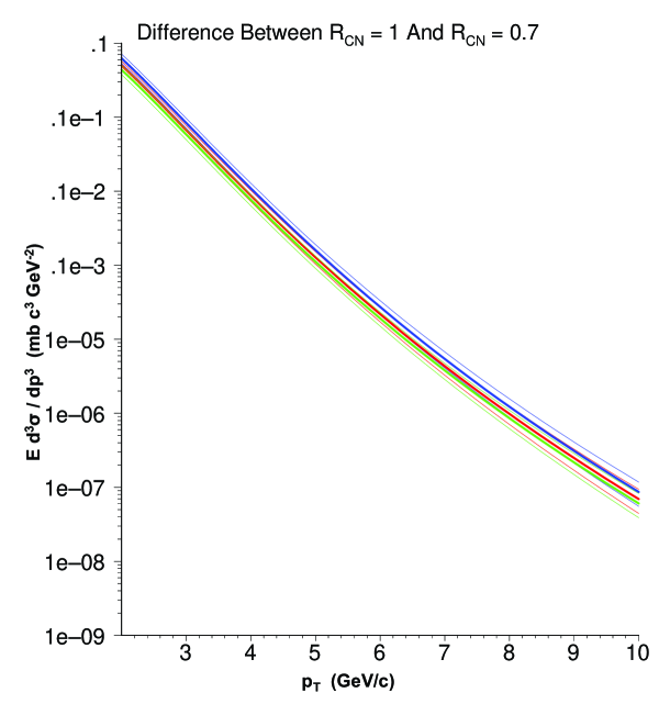
6.2.3 Nuclear Dependency

Nuclear dependency is defined by

$$\sigma_{A}=A^{\alpha}\,\sigma_{N}$$

where $\alpha$ is a function of either $x_{F}$, $p_{T}\;$or both, $A$ is the atomic weight of the material and $N$ is nucleon. E789 studied the production of neutral open charm produced in 800 GeV/c p-A  collisions near $x_{F}=0$. The nuclear dependency reported by this study was $\alpha=1.02\pm 0.03\pm 0.02$, implying that the cross sections scaled as the number of nucleons [8]. In contrast, E866 [23] measured the power $\alpha$ for hidden charm for three regions in $x_{F}$, SXF ($-0.1\leq x_{F}\leq 0.3$), IXF($0.2\leq x_{F}0.6$) and LXF ($0.3\leq x_{F}\leq 0.93$). For this analysis, $0.2\leq x_{F}\leq 0.8$, which lies between the IXF and LXF data from E866. Their results for the power $\alpha(p_{T})$ are shown in Figure 6.21.

The ratio

$$R_{\sigma}=\frac{A_{Be}\,E\,\frac{d^{3}\,\sigma^{\left(p\,Cu\right)}\left(D\,/\,\overline{D}\right)}{d\,p^{3}}\left(p_{T}\right)}{A_{Cu}\,E\,\frac{d^{3}\,\sigma^{(p\,Be)}\left(D\,/\,\overline{D}\right)}{d\,p^{3}}\left(p_{T}\right)}$$

for the 3 parameter $n=6$ results from this analysis are shown in Figure 6.22. The power $\alpha$ can be determined from the ratio of the cross sections, $r=\sigma_{Cu}/\sigma_{Be}$, and the relations $\sigma_{Cu}=A_{Cu}^{\alpha}\,\sigma_{N}$ and $\sigma_{Be}=A_{Be}^{\alpha}\,\sigma_{N}$:

$$\alpha(p_{T})=\frac{1}{\mbox{ln}(A_{Cu})-\mbox{ln}(A_{Be})}\,\mbox{ln}\left(\frac{1}{r}\right)$$

This analysis has extracted $\alpha(p_{T})$ for both ratios ($r(D)$ and $r(\overline{D})$), and the resulting $\alpha(p_{T})$ are shown with the IXF and LXF $J/\Psi$ data from [23] in Figure 6.23. Both ratios used the fits of the 3 parameter $n=6$ to the copper and beryllium data. Based on these results, this analysis concludes that the cross sections, as a function of $p_{T}$, do not simply scale by the atomic weight $A$ (admittedly within large errors, though).

Figure 6.21: $\alpha$ versus $p_{T}\;$for $J/\Psi$ (solid circles) and $\Psi^{\prime}$ (open boxes) production by 800 GeV/c protons. Results are shown for the three data sets - SXF, IXF, and LXF (see text) - which have $\langle x_{F}\rangle=$ 0.055, 0.308 and 0.480 respectively. Only statistical uncertainties are shown. An additional systematic uncertainty of 0.5% is not included. Also shown are the NA3 results at 200 GeV/c [51]. The solid curves represent the parameterization $\alpha(p_{T})=A_{i}(1+0.0604p_{T}+0.0107p^{2}_{T})$, where $A_{i}=$ 0.870, 0.840, 0.782, and 0.881 for the SXF, IXF, LXF data sets, and the NA3 data, respectively. Taken from [23]

Figure 6.22: The ratio of the copper and beryllium $D$ cross sections (black), and the copper and beryllium $\overline{D}$ cross sections (red). Both ratios are normalized to $A_{Be}/A_{Cu}$ and use the results of the fits to the data of the 3 parameter polynomial function with $n=6$. Thin black (red) lines are the scale of the errors of the ratios. Errors include the error of $N$ added in quadrature to the statistical and systematic errors of the other parameters.

Figure 6.23: The power $\alpha(p_{T})$ determined by this analysis for $D+\overline{D}$, where the results from fits using the 3 parameter polynomial with $n=6$ were used as the open charm/anti-charm copper and beryllium cross sections. Red open circles are the IXF data, and the blue open circles are the LXF data taken from [23]. Thin black lines are the errors for $\alpha$ from this analysis. Errors include the error for the parameter $N$ added in quadrature to the error of the remaining parameters.

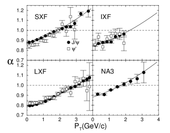
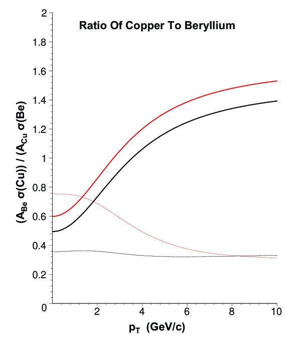
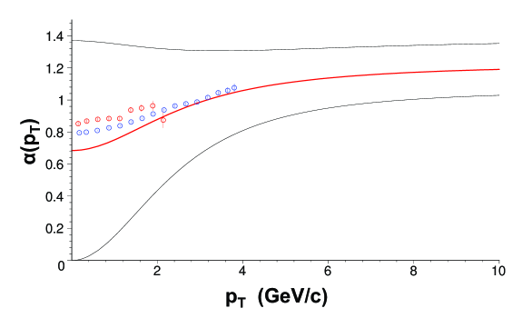
6.3 Summary

The author takes the position that determination of the ’shape’ of the open charm cross sections is more important than determination of the absolute magnitude. Clearly both would be optimal, but the use of secondary spectra required making several assumptions such as the ratio of charged to neutral open charm production. These assumptions provided uncertainties in the absolute magnitudes of the open charm and open anti-charm cross sections that could not be removed.

Single muon data from 800 GeV/c p-Cu  and p-Be  interactions were used to extract the differential open charm/anti-charm cross sections as a function of $p_{T}$. Several functions describing theoretical predictions of the shapes of the cross sections were fit to the data. Monte Carlo studies indicated that the open charm contributions were from open charm hadrons produced with $2.25\leq p_{T}\;\lesssim 7.0$ (GeV/c), $0\lesssim y_{c.m.}\lesssim 2.0$ and $0.2\lesssim x_{F}\lesssim 0.8$. Tables 6.2, 6.3, 6.4 and 6.5 show that the 3 parameter (with $n$ a free parameter or fixed at the integer value 6) and 4 parameter (with the parameter $n$ fixed at the integer value 6) polynomial functions resulted in the smallest $\chi^{2}_{pdf}\;$for both the p-Cu  and p-Be  data. Extrapolation of the results from the 3 parameter function with $n=6$ show good agreement with previous experiments. Fits of the three functions to both the p-Cu  and p-Be  data indicate that the parameter $n$ is very close to 6.0. Due to large correlations introduced by the scaling factor $N$ and loss of data below 2.25 GeV/c, errors for the parameters from fits using the 3 variable function with $n$ a free parameter cannot be determined accurately. In summary:

• The production of open charm hadrons, as a function of the hadron $p_{T}$, is well represented by the function:

  $$\frac{A_{2}}{\left(p_{T}^{2}+\alpha\,m_{c}^{2}\right)^{n}}$$

  with $n=6$. Previous fits using this function have only been reported for $\pi$-A data, where it was found that the same function fit the data well, and $n=5.0$.

• The cross sections can also be well described using the simple exponential

  $$A_{1}\,exp\left(-B\,p_{T}\right)$$

  for $2.25\leq p_{T}\lesssim 8.0$ GeV/c.

• The weighted average value (over $D$ and $\overline{D}$) of $\alpha$ for the 3 parameter function and $n=6$ for p-Cu  production is 3.49 $\pm$ 0.01, while the weighted average for p-Be  production is 2.92 $\pm$ 0.02. The difference indicates that the production via p-Cu  has a steeper slope than p-Be  production for the region in $p_{T}\;$covered by this analysis.

• Extraction of the power $\alpha$ used to relate proton-nucleon cross sections to proton-nucleus cross sections, often referred to as the nuclear dependency, indicates a structure similar to that found for the production of $J/\Psi$, though large uncertainties at low $p_{T}\;$make it difficult to claim that such a structure was found with certainty. Regardless, the author claims that, for the region in $p_{T}\;$for this analysis, the power $\alpha$ continuously rises even if the large errors are taken into account at $p_{T}\;\sim 7.0$ GeV/c. The conclusion reached for this analysis is that the cross sections do not simply scale by the nuclear weight $A$.

Chapter A Miscellaneous Apparatus Information

Table A.1: Drift chamber information. $z$ is given for the average of the two planes for each pair. Chambers are listed in ascending distance along the $z$ axis. All lengths are in inches.

Detector	Angle	Number	Wire		Aperture	Operating
Pair	(deg)	of Wires	Spacing	$z$	($x\times y$)	Voltage
V1-V1′	-14	200	0.250	724.69	48.0 $\times$ 50.0	+1700
Y1-Y1′	0	160	0.250	748.81	48.0 $\times$ 40.0	+1700
U1-U1′	+14	200	0.250	755.48	48.0 $\times$ 50.0	+1700
U2-U2′	+14	160	0.388	1083.40	66.0 $\times$ 62.1	-1950
Y2-Y2′	0	128	0.400	1093.21	66.0 $\times$ 51.2	-2000
V2-V2′	-14	160	0.388	1103.25	66.0 $\times$ 62.1	-2000
U3-U3′	+14	144	0.796	1790.09	106.0 $\times$ 114.7	-2200
Y3-Y3′	0	112	0.820	1800.20	106.0 $\times$ 91.8	-2200
V3-V3′	-14	144	0.796	1810.24	106.0 $\times$ 114.7	-2200

Table A.2: Information on the banks of hodoscopes. Planes are presented in the order in which a particle would traverse them. Minimum and maximum values of $|\overrightarrow{p}_{x}/\overrightarrow{p}_{z}|$ for each $x$ plane are presented for reference, and are based on disconnecting the high voltage supplies to the middle half of each bank as shown in figures 2.3 and 2.4. All lengths are in inches.

		Number	Scint.	Aperture	$\mbox{TAN}\theta_{x}\,$	$\mbox{TAN}\theta_{x}\,$
Det.	$z$	Scint.	Width	$x\times y$	Min	Max
Y1	769.78	16	2.5	47.50 $\times$ 40.75
X1	770.72	12	4.0	47.53 $\times$ 40.78	0.015	0.030
Y2	1114.94	16	3.0	64.625 $\times$ 48.625
X3	1822.00	12	8.68	105.18 $\times$ 92.0	0.014	0.030
Y3	1832.00	13	7.5	104.00 $\times$ 92.0
Y4	2035.50	14	8.0	116.00 $\times$ 100.00
X4	2131.12	16	7.125	126.00 $\times$ 114.00	0.015	0.030

Table A.3: Information for the three layers of proportional tubes in Station 4 as used in taking data for this analysis. Layers are listed in ascending distance from the origin. All lengths are in inches.

	Number	Cell	Aperture		Operating
Bank	of Tubes	($x\times y$)	($x\times y$)	$z$	Voltage
PT-Y1	120	1.00 $\times$ 1.00	117.0 $\times$ 120.0	2041.75	+2500
PT-X	135	1.00 $\times$ 1.00	135.4 $\times$ 121.5	2135.88	+2500
PT-Y2	143	1.00 $\times$ 1.00	141.5 $\times$ 143.0	2200.75	+2500

Figure A.1: Block diagram of the E866 trigger system for the left hand side. Taken from [16]

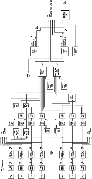
Chapter B Analysis

Table B.1: Estimated fraction of events in the target analysis of Run 2751 that originated in the dump. Dump IC3SB is the fraction of the luminosity that survived the target and interacted in the dump. Totals are for the three targets only.

Target	Total	Dump	Estimated	Number	Fraction
	IC3SB	IC3SB	Dump	Events	Dump
			Events		Events
0	40661	40661	143 $\pm$ 12	143	1.000
1	53013	48708	170 $\pm$ 15
2	52872	46663	163 $\pm$ 14
3	27225	22983	80 $\pm$ 7
Total	133110	118324	413 $\pm$ 22	6350 $\pm$ 80	0.065 $\pm$ 0.004

Table B.2: Spectrometer calibrations for data taken with the magnetic fields in SM12 and SM3 parallel. All target analyses used $Z_{tgt}=-24.0$ and $Z_{scat}=200.0$ inches. All dump analyses used $Z_{tgt}=85.1$ and $Z_{scat}=235.0$ inches.

Run		$TWEE$	$X0$	$Y0$	$\theta_{x}^{\prime}$	$\theta_{y}^{\prime}$
			(in)	(in)	(rad)	(rad)
2748	Target	0.993	0.040	-0.525	0.00015	-0.00025
	Dump	0.995	0.046	-0.560	0.00008	-0.00015
2749	Target	0.995	0.051	-0.538	0.00010	-0.00035
	Dump	0.997	0.063	-0.572	0.00005	0.00000
2750	Target	0.990	0.070	-0.540	0.00010	-0.00035
	Dump	0.992	0.081	-0.572	0.00008	0.00004
2751	Target	0.990	0.007	-0.563	0.00005	-0.00035
	Dump	0.992	0.024	-0.585	0.00005	0.00004
2752	Target	0.990	0.032	-0.553	0.00005	-0.00035
	Dump	0.992	0.051	-0.575	0.00000	0.00004
2753	Target	0.990	0.050	-0.555	0.00005	-0.00035
	Dump	0.992	0.056	-0.578	0.00000	0.00004
2754	Target	0.988	0.035	-0.549	0.00005	-0.00035
	Dump	0.990	0.054	-0.583	0.00000	0.00000
2755	Target	0.986	0.040	-0.569	0.00005	-0.00035
	Dump	0.990	0.049	-0.593	0.00005	-0.00015
2756	Target	0.986	0.049	-0.545	0.00001	-0.00035
	Dump	0.990	0.072	-0.581	0.00000	-0.00005
2757	Target	0.986	0.045	-0.547	0.00001	-0.00035
	Dump	0.990	0.066	-0.581	-0.00002	-0.00008

Chapter C $\chi^{2}\;$From The Minimizations

C.1 Sub-Total And Total $\chi^{2}$

Table C.1: The eight sub-total, total, number of degrees of freedom and reduced $\chi^{2}$, $\chi^{2}_{pdf}\;$for all minimizations to the copper target data. Top line gives the individual spectra sub-totals, and the second line gives the sub-totals by charge and production region.

Copper Data
		$\chi^{2}_{T^{+}}$	$\chi^{2}_{T^{-}}$	$\chi^{2}_{D^{+}}$	$\chi^{2}_{D^{-}}$
Function	$n$	$\chi^{2}_{+}$	$\chi^{2}_{-}$	$\chi^{2}_{T}$	$\chi^{2}_{D}$	$\chi^{2}$	$ndf$	$\chi^{2}_{pdf}$
		18.43	21.68	16.90	24.41
$A_{1}\,exp\left(-B\,p_{T}\right)$	NA	35.33	46.09	40.11	41.31	81.42	61	1.33
		12.28	18.40	10.65	12.25
	FF	22.94	31.16	31.19	22.91	54.09	59	0.92
		39.72	48.38	133.36	83.95
	4	173.08	132.32	88.10	217.31	305.41	61	5.01
		15.04	23.89	35.44	25.21
	5	50.48	49.10	38.93	60.65	99.58	61	1.63
$\frac{\displaystyle A_{2}}{\displaystyle\left(p_{T}^{2}+\alpha\,m_{c}^{2}\right)^{n}}$		11.98	18.96	12.80	12.33
	6	24.78	31.29	30.94	25.14	56.08	61	0.92
		13.71	18.31	11.59	14.87
	4	25.30	33.18	32.03	26.46	58.48	59	0.99
		12.32	19.14	10.44	12.70
	5	22.76	31.85	31.47	23.15	54.61	59	0.93
		12.52	18.94	10.45	12.32
$A_{2}\,\frac{\displaystyle\left(1-p_{T}\,/\,p_{beam}\right)^{m}}{\displaystyle\left(p_{T}^{2}+\alpha\,m_{c}^{2}\right)^{n}}$	6	22.96	31.26	31.46	22.76	54.23	59	0.92

Table C.2: The eight sub-total, total, number of degrees of freedom and reduced $\chi^{2}$, $\chi^{2}_{pdf}\;$for all minimizations to the beryllium target data. Top line gives the individual spectra sub-totals and the second line gives the sub-totals by charge and production region.

Beryllium Data
		$\chi^{2}_{T^{+}}$	$\chi^{2}_{T^{-}}$	$\chi^{2}_{D^{+}}$	$\chi^{2}_{D^{-}}$
Function	$n$	$\chi^{2}_{+}$	$\chi^{2}_{-}$	$\chi^{2}_{T}$	$\chi^{2}_{D}$	$\chi^{2}$	$ndf$	$\chi^{2}_{pdf}$
		9.55	7.44	12.71	33.18
$A_{1}\,exp\left(-B\,p_{T}\right)$	NA	22.26	40.62	16.99	45.89	62.88	63	1.00
		7.58	6.69	12.94	32.93
	FF	20.52	39.62	14.27	45.87	60.14	61	0.95
		65.08	56.19	13.65	32.40
	4	78.73	88.60	121.27	46.06	167.32	63	2.66
		17.59	20.76	12.34	33.73
	5	29.94	54.40	38.36	46.08	84.44	63	1.34
$\frac{\displaystyle A_{2}}{\displaystyle\left(p_{T}^{2}+\alpha\,m_{c}^{2}\right)^{n}}$		7.76	8.54	12.76	33.12
	6	20.52	41.66	16.30	45.88	62.19	63	0.99
		7.28	6.15	12.91	32.96
	4	20.18	39.12	13.43	45.87	59.30	61	0.97
		6.69	5.88	12.91	32.96
	5	19.60	38.84	12.57	45.87	58.44	61	0.96
		6.59	5.79	12.90	32.97
$A_{2}\,\frac{\displaystyle\left(1-p_{T}\,/\,p_{beam}\right)^{m}}{\displaystyle\left(p_{T}^{2}+\alpha\,m_{c}^{2}\right)^{n}}$	6	19.49	38.76	12.38	45.87	58.25	61	0.95

References

- [1] S. Eidelman, et al., Phys. Lett. B592, 1 (2004).
- [2] A. D. Martin, et al., Eur. Phys. J. C28, 455 (2003).
- [3] A. D. Martin, et al., Eur. Phys. J. C23, 73 (2002).
- [4] Michelangelo L. Mangano, hep-ph/9711337 (1997).
- [5] S. Frixione, M. Mangano, P. Nason and G.Ridolfi, hep-ph/9702287 (1997).
- [6] R. Ammar, et al., Phys. Rev. Lett. 61, 2185 (1988).
- [7] K. Kodama, et al., Phys. Lett. B263, 573 (1991).
- [8] M. J. Leitch, et al., Phys. Rev. Lett. 72, 2542 (1994).
- [9] G. A. Alves, S. Amato, et al., Phys. Rev. Lett. 77, 2392 (1996).
- [10] G. A. Alves, S. Amato, et al., Phys. Rev. Lett. 77, 2388 (1996).
- [11] M. Mangano, P. Nason, and G. Rudolfi, Nucl. Phys. B405, 507 (1993).
- [12] Matteo Cacciari and Paolo Nason, hep-ph/0306212 (2003).
- [13] U. Husemann for the HERA Collaboration, hep-ex/0408110 (2004).
- [14] Haibin Zhang (for the STAR Collaboration), nucl-ex/0410038 (2004).
- [15] M. S. Kowitt, Ph.D. Thesis, Chapter 2, University of California at Berkeley, 1992.
- [16] E. A. Hawker, Ph.D. Dissertation, Chapter 2, Texas A&M University, 1998.
- [17] R. S. Towell, Ph.D. Dissertation, Chapter 3, University of Texas at Austin, 1999.
- [18] T. H. Chang, Ph.D. Dissertation, Chapter 2, New Mexico State University, 1999.
- [19] Bill Lee, Ph.D. Dissertation, Georgia State University, 1999.
- [20] Jason Webb, Ph.D. Dissertation, New Mexico State University, 2002. Results still not considered final.
- [21] E. A. Hawker, et al., Phys. Rev. Lett. 80, 3715 (1998).
- [22] M. A. Vasiliev, et al., Phys. Rev. Lett. 83, 2304 (1999).
- [23] M. J. Leitch, et al., Phys. Rev. Lett. 84, 3256 (2000).
- [24] C. N. Brown, et al., Phys. Rev. Lett. 86, 2529 (2001).
- [25] R. S. Towell, et al., Phys. Rev. D64, 052002 (2001).
- [26] T. H. Chang, et al., Phys. Rev. Lett. 91, 211801 (2003).
- [27] J. C. Webb, et al., hep-ex/0302019 (2003).
- [28] C. A. Gagliardi, E. A. Hawker, R. E. Tribble, D. Koetke, P. M. Nord, P. L. McGaughey, and C. N. Brown, Nucl. Instrum. Methods, A 418, 322 (1998).
- [29] D. M. Kaplan, Introduction to the E605 Readout System, E605 Memorandum, 10 August, 1982 (unpublished).
- [30] A. Van Ginneken, Nucl. Instr. Meth. A 251, 21-39 (1986).
- [31] G. Moreno, C. N. Brown, et al., Phys. Rev. D 43, 2815 (1991).
- [32] B. Alper, H. Böggild, et al., Nucl. Phys. B100, 237 (1975).
- [33] J. W. Cronin, et al. (Chicago-Princeton Collaboration), Phys. Rev. D 11, 3105 (1975).
- [34] D. Antreasyan, J. W. Cronin, H. J. Frisch, et al., Phys. Rev. D 19, 764 (1979).
- [35] A. S. Carroll, I-H. Chiang, T. F. Kycia, et al., Phys. Lett. 80B, 319 (1979).
- [36] H. L. Lai and W. K. Tung, hep-ph/9701256 (1997).
- [37] R. Vogt and S. J. Brodsky, Nucl. Phys. B438, 261 (1995).
- [38] S. J. Brodsky and G. R. Farrar, Phys. Rev. Lett. 31, 1153 (1973).
- [39] R. Blankenbecler and S. J. Brodsky, Phys. Rev. D 10, 2973 (1974).
- [40] R. Blankenbecler, S. J. Brodsky and J. Gunion, Phys. Rev. D 12, 3469 (1975).
- [41] J. A. Appel, M. H. Bourquin, et al., Phys. Rev. Lett. 33, 719 (1974).
- [42] Louis Lyons, Statistics for nuclear and particle physicists, Cambridge University Press, 1989.
- [43] F. James, MINUIT, Function Minimization and Error Analysis, CERN Program Library D506, 1998.
- [44] Jeffrey A. Appel, hep-ex/0011101 (2000).
- [45] W. Melnitchouk, et al., hep-ph/9707387 (1997).
- [46] R. Vogt and S. J. Brodsky, Nucl. Phys. B478, 311 (1996).
- [47] CERNLIB and related software as well as documentation can be found at http://wwwinfo.cern.ch/asd/.
- [48] M. Aguilar-Benitez, et al. (LEBC-EHS Collaboration), Z. Phys. C40, 321, (1988).
- [49] S. Frixione, M. Mangano, P. Nason and G. Ridolphi, Nucl. Phys. B431, 453 (1994).
- [50] D. M. Alde et al. (E772), Phys. Rev. Lett. 66, 133 (1991).
- [51] J. Badier et al., Z. Phys. C20, 101 (1983).
- [52] Private communications from Paul Reimer.