Measurement of $D_{s}^{+}\to\mu^{+}\nu$ and the Decay Constant $f_{D_{s}}$  

Abstract

We examine $e^{+}e^{-}\to D_{s}^{-}D_{s}^{*+}$ or $D_{s}^{-*}D_{s}^{+}$ collisions at 4170 MeV using the CLEO-c detector in order to measure the decay constant $f_{D_{s}^{+}}$. We use the $D_{s}^{+}\to\ell^{+}\nu$ channel, where the $\ell^{+}$ designates either a $\mu^{+}$ or a $\tau^{+}$. Analyzing both modes simultaneously, we determine ${\cal{B}}(D_{s}^{+}\to\mu^{+}\nu)=(0.657\pm 0.090\pm 0.028)$%, ${\cal{B}}(D_{s}^{+}\to\tau^{+}\nu)=(7.1\pm 1.4\pm 0.3)$%, and extract $f_{D_{s}^{+}}=282\pm 16\pm 7{~{}\rm MeV}$. Combining with our previous determination of ${\cal{B}}(D^{+}\to\mu^{+}\nu)$, we find that the ratio $f_{D_{s}^{+}}/f_{D^{+}}=1.27\pm 0.12\pm 0.03$. (All new results here are preliminary.) We compare with current theoretical estimates.

I Introduction

To extract precise information on the size of Cabibbo-Kobayashi-Maskawa matrix elements from $B-\overline{B}$ mixing measurements the ratio of “leptonic decay constants,” $f_{i}$ for $B_{d}$ and $B_{s}$ mesons must be well known formula-mix . Indeed, the recent measurement of $B_{s}^{0}-\overline{B}_{s}^{0}$ mixing by CDF CDF that can now be compared to the very well measured $B^{0}$ mixing PDG , has pointed out the urgent need for precise numbers Belle-taunu . The $f_{i}$ have been calculated theoretically. The most promising of these calculations are based on lattice-gauge theory that include the light quark loops Davies . In order to ensure that these theories can adequately predict $f_{B_{s}}/f_{B_{d}}$ it is useful to check the analogous ratio from charm decays $f_{D^{+}_{s}}/f_{D^{+}}$. We have previously measured $f_{D^{+}}$ our-fDp ; DptomunPRD . Here we present the most precise measurement to date of $f_{D_{s}^{+}}$ and the ratio $f_{D_{s}^{+}}/f_{D^{+}}$.

The only way in the Standard Model (SM) for a $D_{s}$ meson to decay purely leptonically, via annihilation through a virtual $W^{+}$, is shown in Fig. 1. The decay rate is given by Formula1

$$\Gamma(D_{s}^{+}\to\ell^{+}\nu)={{G_{F}^{2}}\over 8\pi}f_{D_{s}^{+}}^{2}m_{\ell}^{2}M_{D_{s}^{+}}\left(1-{m_{\ell}^{2}\over M_{D_{s}^{+}}^{2}}\right)^{2}\left|V_{cs}\right|^{2}~{}~{}~{},$$ (1)

where $M_{D_{s}^{+}}$ is the $D_{s}^{+}$ mass, $m_{\ell}$ is the mass of the charged final state lepton, $V_{cs}$ is a Cabibbo-Kobayashi-Maskawa matrix element with a value we take equal to 0.9737 PDG , and $G_{F}$ is the Fermi coupling constant.

Figure 1: The decay diagram for $D_{s}^{+}\to\ell^{+}\nu$.

Previous measurements of $f_{D_{s}^{+}}$ have been hampered by a lack of statistical precision, and relatively large systematic errors PDG . One large systematic error source has been the lack of knowledge of the absolute branching ratio for $D_{s}^{+}\to\phi\pi^{+}$, the mode which most measurements have used for normalization stone-fpcp . The results we report here will not have this problem.

In this paper we analyze both $D_{s}\to\mu^{+}\nu$ and $D_{s}\to\tau^{+}\nu$, $\tau^{+}\to\pi^{+}\overline{\nu}$. Both $D_{s}$ decays are helicity suppressed because the $D_{s}$ is a spin-0 particle, and the final state consists of a naturally left-handed spin-1/2 neutrino and a naturally right-handed spin-1/2 anti-lepton that have equal energies and opposite momenta. The ratio of decay rates for any two different leptons is then fixed by well-known masses. For example, for $\tau^{+}\nu$ to $\mu^{+}\nu$, the expected ratio is

$$R\equiv\frac{\Gamma(D_{s}^{+}\to\tau^{+}\nu)}{\Gamma(D_{s}^{+}\to\mu^{+}\nu)}={{m_{\tau^{+}}^{2}\left(1-{m_{\tau^{+}}^{2}\over M_{D_{s}^{+}}^{2}}\right)^{2}}\over{m_{\mu^{+}}^{2}\left(1-{m_{\mu^{+}}^{2}\over M_{D_{s}^{+}}^{2}}\right)^{2}}}~{}~{}.$$ (2)

Using measured masses PDG , this expression yields a value of 9.72 with a negligibly small error. After multiplying by ${\cal{B}}(\tau^{+}\to\pi^{+}\overline{\nu}$ of 11.06%, the ratio is 1.076 for $\tau^{+}\nu$ with respect to $\mu^{+}\nu$, when $\tau^{+}\to\pi^{+}\overline{\nu}$.

II Experimental Method

II.1 Selection of $D_{s}$ Candidates

The CLEO-c detector is equipped to measure the momenta and directions of charged particles, identify them using specific ionization (dE/dx) and Cherenkov light (RICH), detect photons and determine their directions and energies CLEODR .

In this study we use 200 pb^-1 of data produced in $e^{+}e^{-}$ collisions using the Cornell Electron Storage Ring (CESR) and recorded near 4.170 GeV. Here the cross-section for $D_{s}^{*+}D_{s}^{-}$+$D_{s}^{+}D_{s}^{*-}$ is $\sim$1 nb, with $D_{s}^{+}D_{s}^{-}$ production being only $\sim$5% of this rate DsDsCBX . $D$ mesons are also produced mostly as $D^{*}\overline{D^{*}}$, with a cross-section of $\sim$5 nb, and in $D^{*}\overline{D}+D\overline{D^{*}}$ final states with a cross-section of $\sim$2 nb. The $D\overline{D}$ is a relatively small $\sim$0.2 nb poling . There also appears to be $D\overline{D}$ production with extra pions. The underlying light quark “continuum” background is about 12 nb. The relatively large cross-sections, relatively large branching ratios and sufficient luminosities, allow us to fully reconstruct one $D_{s}$ as a “tag,” and examine the properties of the other. In this paper we designate the tag as a $D_{s}^{-}$ and examine the leptonic decays of the $D_{s}^{+}$, though in reality we use both charges. Track selection, particle identification, $\gamma$, $\pi^{0}$, $K_{S}$ and muon selection cuts are identical to those described in Ref. our-fDp .

The events we use here occur when $e^{+}e^{-}\to D_{s}^{*+}D_{s}^{-}$ or $D_{s}^{+}D_{s}^{*-}$. We will reconstruct tags from both final states. The beam constrained mass, $m_{BC}$, is formed by using the beam energy to construct the mass our-fDp . If we do not detect the photon and reconstruct the $m_{BC}$ distribution, we obtain the distribution from Monte Carlo shown in Fig. 2. The narrow peak occurs when the reconstructed $D_{s}$ does not come from the $D_{s}^{*}$ decay.

Figure 2: The beam constrained mass $m_{BC}$ from Monte Carlo simulation of $e^{+}e^{-}\to D_{s}^{+}D_{s}^{*-}$, $D_{s}^{\pm}\to\phi\pi^{\pm}$ at 4170 MeV. The narrow peak is from the $D_{s}^{+}$ and the wider one from the $D_{s}^{-}$. (The distributions are not centered at the $D_{s}^{+}$ or $D_{s}^{*+}$ masses, because the reconstructed particles are assumed to have the energy of the beam.)

Rather than selecting events based on $m_{BC}$, we first select an interval that accepts most of the events, $2.015>m_{BC}>2.067$ GeV, and examine the invariant mass. Distributions from data for the 8 modes we use in this analysis are shown in Fig. 3. Note that the resolution in invariant mass is excellent, and the backgrounds not very large, at least in these modes. To determine the number of tags we fit the invariant mass distributions to the sum of two Gaussians centered at the $D_{s}^{-}$ mass. The r.m.s. resolution ($\sigma$) is defined as

$$\sigma=f_{1}\sigma_{1}+(1-f_{1})\sigma_{2},$$ (3)

where $\sigma_{1}$ and $\sigma_{2}$ are the individual widths of the two Gaussians and $f_{1}$ is the fractional area of the first Gaussian. The number of tags in each mode is listed in Table 1.

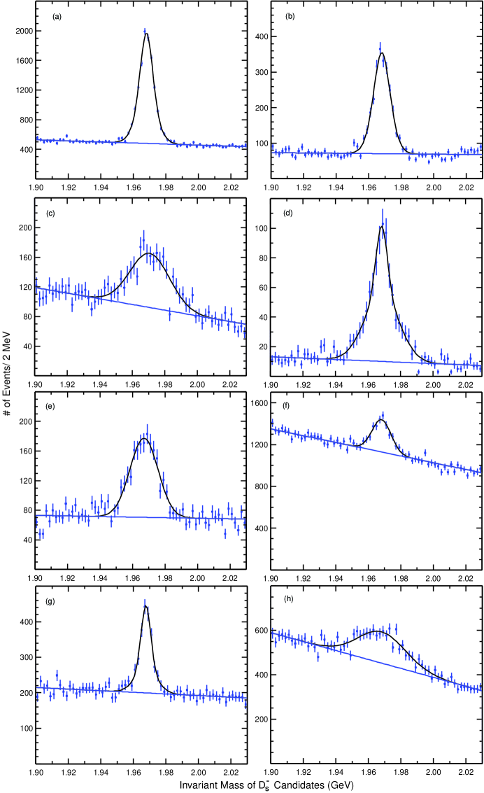
Figure 3: Invariant mass of $D_{s}^{-}$ candidates (a) $K^{+}K^{-}\pi^{+}$, (b) $K_{S}K^{+}$, (c) $\eta\pi^{+}$, (d) $\eta^{\prime}\pi^{+}$, (e) $\phi\rho^{+}$, (f) $\pi^{+}\pi^{-}\pi^{+}$, (g) $K^{*+}K^{*0}$, (h) $\eta\rho^{+}$, after requiring the total energy to be consistent with the beam energy. The curves are fits to two-Gaussian signal functions plus a linear background.

Table 1: Tagging modes and numbers of signal and background events, within $\pm 2.5\sigma$ for all modes, except $\eta\rho^{+}$ ($\pm 2\sigma$), from two-Gaussian fits to the invariant mass plots.

Mode	#	Background
$K^{+}K^{-}\pi^{+}$	$8446\pm 160$	6792
$K_{S}K^{+}$	1852$\pm$62	1021
$\eta\pi^{+}$; $\eta\to\gamma\gamma$	$1101\pm 80$	2803
$\eta^{\prime}\pi^{+}$; $\eta^{\prime}\to\pi^{+}\pi^{-}\eta$, $\eta\to\gamma\gamma$	786$\pm$37	242
$\phi\rho^{+}$; $\phi\to K^{+}K^{-}$, $\rho^{+}\to\pi^{+}\pi^{0}$	1140$\pm$59	1515
$\pi^{+}\pi^{-}\pi^{+}$	2214$\pm$156	15668
$K^{*+}K^{*0}$; $K^{*+}\to K_{S}\pi^{+}$, $K^{*0}\to K^{-}\pi^{+}$	1197$\pm$81	2955
$\eta\rho^{+}$; $\eta\to\gamma\gamma$, $\rho^{+}\to\pi^{+}\pi^{0}$	2449$\pm$185	13043
Sum	$19185\pm 325$	44039

II.2 Procedure for Finding Leptonic Decays

In this analysis we will be selecting events from two processes one where $D_{s}^{+}\to\mu^{+}\nu$ and the other when $D_{s}^{+}\to\tau^{+}\nu$, $\tau^{+}\to\pi^{+}\overline{\nu}$. We first have to select a sample of tag events. We require the invariant masses, shown in Fig. 3 to be within $\pm~{}2.5\sigma$ of the known $D_{s}^{-}$ mass (here $\sigma$ is the r.m.s. width). Then we look for an additional photon candidate in the event that satisfies our shower shape requirement. Regardless of whether or not the photon forms a $D_{s}^{*}$ with the tag, for real $D_{s}^{*}D_{s}$ events, the missing mass squared, MM^∗2 recoiling against the photon and the $D_{s}^{-}$ tag should peak at the $D_{s}^{+}$ mass. We calculate

$${\rm MM}^{*2}=\left(E_{\rm CM}-E_{D}-E_{\gamma}\right)^{2}-\left(-\overrightarrow{p_{D}}-\overrightarrow{p_{\gamma}}\right)^{2},$$ (4)

where $E_{\rm CM}$ is the center of mass energy, $E_{D}$ ($\overrightarrow{p_{D}}$) is the energy (momentum) of the fully reconstructed $D_{s}^{-}$ tag, $E_{\gamma}$ ($\overrightarrow{p_{\gamma}}$) is the energy (momentum) of the additional photon. In performing this calculation we use a kinematic fit that constrains the decay products of the $D_{s}^{-}$ to the known $D_{s}$ mass and conserves overall momentum and energy. All photons in the event are used, except for those that are decay products of the $D_{s}^{-}$ candidate.

The MM^∗2 from the $D_{s}^{-}$ tag sample data is shown in Fig. 4. We fit this distribution to determine the number of tag events. This procedure is enhanced by having information on the shape of the signal function. One possibility is to use the Monte Carlo simulation for this purpose. Our relatively large sample of fully reconstructed $D^{*0}D^{0}$ events allows us to examine the signal shape in data when one neutral $D$ is ignored. This sample is shown in Fig. 5. The signal is fit to a Crystal Ball function CBL ; taunu . The $\sigma$ parameter, that represents the width of the distribution, is found to be 0.039$\pm$0.02 GeV² compared with the Monte Carlo estimate of 0.310$\pm$0.003 GeV². The Monte Carlo does not reproduce well the width of the distribution, so we do not use it here. The energy of photons from the $D^{0}$ and $D_{s}$ events are somewhat different due to the different masses of the parent hadrons. Thus we cannot use the $\sigma$ found here directly. We do, however, get an estimate of the parameters of the tail of the distribution.

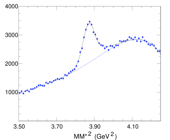
Figure 4: The MM*² distribution from events with a photon in addition to the $D_{s}^{-}$ tag. The curve is a fit to the Crystal Ball function and a 5th order Chebychev background function.

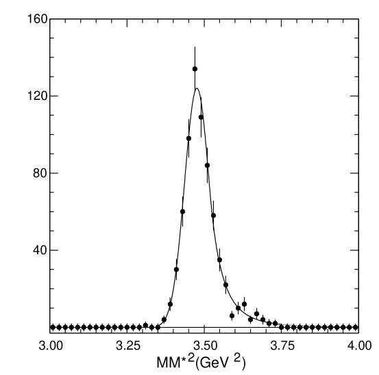
Figure 5: The MM*² distribution from a sample of fully reconstructed $D^{*0}D^{0}$ events where one $D^{0}$ is ignored. The curve is a fit to the Crystal Ball function.

Using the fixed tail parameters of the Crystal Ball function, and a 5th order Chebyshev polynomial background, we find 12604$\pm$423 signal events. After selecting events within an interval $3.978>$MM${}^{*2}>3.776$ GeV², we are left with 11880$\pm$399 events. A systematic error of 3% is assigned by seeing how the event yields vary when the width of the distribution is changed by $\pm 1\sigma$ and an additional systematic error of 3% is added in quadrature from changing the form of the background function and the fit range. There is also a small enhancement of 4% on our ability to find tags in $\mu^{+}\nu$ (or $\tau^{+}\nu$, $\tau^{+}\to\pi^{+}\overline{\nu}$) events as compared with generic events to which we assign a 10% systematic error or $\pm$0.4%, again added in quadrature.

We next describe the search for $D_{s}^{+}\to\mu^{+}\nu$. Candidate events are searched for by selecting events with only a single extra track with opposite sign of charge to the tag, and also require that there not be an extra neutral energy cluster in excess of 300 MeV. Since here we are searching for events where there is a single missing neutrino, the missing mass squared, MM², evaluated by taking into account the seen $\mu^{+}$, $D_{s}^{-}$, and the $\gamma$ should peak at zero; the MM² is computed as

$${\rm MM}^{2}=\left(E_{\rm CM}-E_{D}-E_{\gamma}-E_{\mu}\right)^{2}-\left(-\overrightarrow{p_{D}}-\overrightarrow{p_{\gamma}}-\overrightarrow{p_{\mu}}\right)^{2},$$ (5)

where $E_{\rm CM}$ is the center of mass energy, $E_{D}$ ($\overrightarrow{p_{D}}$) is the energy (momentum) of the fully reconstructed $D_{s}^{-}$ tag, $E_{\gamma}$ ($\overrightarrow{p_{\gamma}}$) is the energy (momentum) of the additional photon, and $E_{\mu}$ ($\overrightarrow{p_{\mu}}$) is the energy (momentum) of the candidate muon track.

We also make use of a set of kinematical constraints and fit each event to two hypotheses one of which is that the $D_{s}^{-}$ tag is the daughter of a $D_{s}^{*-}$ and the other that the $D_{s}^{*+}$ decays into $\gamma D_{s}^{+}$, with the $D_{s}^{+}$ subsequently decaying into $\mu^{+}\nu$. The hypothesis with the lowest $\chi^{2}$ is kept. If there is more than one photon candidate in an event we choose only the lowest $\chi^{2}$ choice among all the candidates and hypotheses.

The kinematical constraints are

$$\overrightarrow{p}_{\!D_{s}}+\overrightarrow{p}_{\!D_{s}^{*}}=0$$ (6)

$$E_{\rm CM}=E_{D_{s}}+E_{D_{s}^{*}}$$

$$E_{D_{s}^{*}}=\frac{E_{\rm CM}}{2}+\frac{M_{D_{s}^{*}}^{2}-M_{D_{s}}^{2}}{2E_{\rm CM}}{\rm~{}or~{}}E_{D_{s}}=\frac{E_{\rm CM}}{2}-\frac{M_{D_{s}^{*}}^{2}-M_{D_{s}}^{2}}{2E_{\rm CM}}$$

$$M_{D_{s}^{*}}-M_{D_{s}}=143.6{\rm~{}MeV}.$$

In addition, we constrain the invariant mass of the $D_{s}^{-}$ tag to the known $D_{s}$ mass. This gives us a total of 7 constraints. The missing neutrino four-vector needs to be determined, so we are left with a three-constraint fit. We preform a standard iterative fit minimizing $\chi^{2}$. As we do not want to be subject to systematic uncertainties that depending on understanding the absolute scale of the errors, we do not make a $\chi^{2}$ cut but simply choose the photon and the decay sequence in each event with the minimum $\chi^{2}$.

III Signal Reconstruction

In this analysis, we consider three separate cases: (i) the track deposits $<$ 300 MeV in the calorimeter, characteristic of a non-interacting pion or a muon; (ii) the track deposits $>$ 300 MeV in the calorimeter, characteristic of an interacting pion; (iii) the track satisfies our electron selection criteria defined below. Then we separately study the MM² distributions for these three cases. The separation between muons and pions is not unique. Case (i) contains 99% of the muons but also 60% of the pions, while case (ii) includes 1% of the muons and 40% of the pions DptomunPRD . Case (iii) does not include any signal but is used later for background estimation.

We exclude events with more than one additional, opposite-sign charged track in addition to the tagged $D_{s}^{-}$, or with extra neutral energy. Specifically, we veto events with extra charged tracks arising from the event vertex or having a maximum neutral energy cluster, consistent with being a photon, of more than 300 MeV. These cuts are highly effective in reducing backgrounds. The photon energy cut is especially useful to reject $D_{s}^{+}\to\pi^{+}\pi^{0}$ decays, should this mode be significant, and $\eta\pi^{+}$ decays.

The track candidates are required to be within the barrel region of the detector $|\cos\theta|<0.81$, where $\theta$ is the angle with respect to the beam. For cases (i) and (ii) we insist that the track not be identified as a kaon. For electron identification we require a match between the momentum measurement in the tracking system and the energy deposited in the CsI calorimeter and the shape of the energy distribution among the crystals is consistent with that expected for an electromagnetic shower.

III.1 The Expected MM² Spectrum

For the $\mu^{+}\nu$, final state the MM² distribution can be modelled as the sum of two-Gaussians centered at zero (see Eq. 3) A Monte Carlo simulation of the MM² for the $\phi\pi^{+}$ subset of $K^{+}K^{-}\pi^{+}$ tags is shown in Fig. 6 both before and after the fit. The fit changes the resolution $\sigma$=0.032 GeV² to 0.025 GeV², a 22% improvement, and there is no loss of events.

Figure 6: The MM² resolution from Monte Carlo simulation for $D_{s}^{+}\to\mu^{+}\nu$ utilizing a $\phi\pi^{+}$ tag and a $\gamma$ from either $D_{s}^{*}$ decay, both before the kinematic fit (a) and after (b).

We check the resolution using data. The mode $D_{s}^{+}\to K^{0}K^{+}$ provides an excellent testing ground. We search for events with at least one additional track identified as kaon using the RICH detector, in addition to a $D_{s}^{-}$ tag. The MM² distribution is shown in Fig. 7. Fitting this distribution to a two-Gaussian shape gives a MM² resolution of 0.025 GeV² in agreement with Monte Carlo simulation.

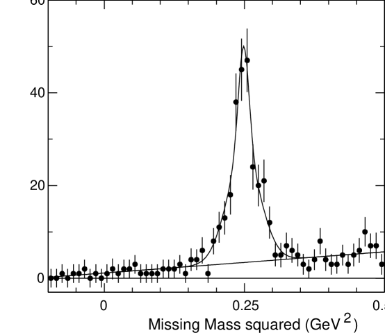
Figure 7: The MM² distribution for events with a identified $K^{+}$ track. The kinematic fit has been applied. The curve is a fit to the sum of two-Gaussians centered at the square of the $\overline{K}^{0}$ mass and a linear background.

For the $\tau^{+}\nu$, $\tau^{+}\to\pi^{+}\nu$ final state a Monte Carlo simulation of the MM² spectra is shown in Fig. 8. The extra missing neutrino results in a smeared distribution.

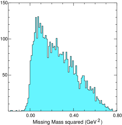
Figure 8: The MM² distribution for $D_{s}^{+}\to\tau^{+}\nu$, $\tau^{+}\to\pi^{+}\overline{\nu}$ at 4170 MeV.

III.2 MM² Spectra in Data

Figure 9: The MM² distributions from data using $D_{s}^{-}$ tags and one additional opposite-sign charged track and no extra energetic showers (see text). For the case when the single track (a) deposits $<$ 300 MeV of energy in the calorimeter, case (i). The peak near zero is from $D_{s}^{+}\to\mu^{+}\nu$ events. (b) Track deposits $>$ 300 MeV in crystal calorimeter but is not consistent with being an electron, case (ii). (c) The track is identified as an electron case (iii).

The MM² distributions from data are shown in Fig. 9. Case (i) requires that the candidate muon track deposit $<$300 MeV of energy in the calorimeter, consistent with a non-interacting track. Case (ii) requires just the opposite, that the track deposit $>$ 300 MeV and also not be consistent with being an electron. Case (iii) requires that the track be consistent with being an electron. The overall signal region we consider are below MM² of 0.20 GeV². Otherwise we admit background from $\eta\pi^{+}$ and $K^{0}\pi^{+}$ final states. There is a clear peak in Fig. 9(a), due to $D_{s}^{+}\to\mu^{+}\nu$. Furthermore the region between $\mu^{+}\nu$ peak and 0.20 GeV² has events that we will show are dominantly due to the $\tau^{+}\nu$ decay.

The specific signal regions are defined as follows: for $\mu^{+}\nu$, $0.05>$MM${}^{2}>-0.05$ GeV², corresponding to $\pm 2\sigma$ or 95% of the signal; for $\tau\nu$, $\tau^{+}\to\pi^{+}\overline{\nu}$, in case (i) $0.20>$MM${}^{2}>0.05$ GeV² and in case (ii) $0.20>$MM${}^{2}>-0.05$ GeV². In these regions we find 64, 24 and 12 events, respectively.

III.3 Background Evaluations

We consider the background arising from two sources: one from real $D_{s}^{+}$ decays and the other from the background under the single-tag signal-peaks. For the latter, we obtain the background from data. We define side-bands of the invariant mass signals shown in Fig. 2 in intervals approximately 4-5$\sigma$ on the low and high sides of the invariant mass peaks for all modes. Thus the amount of data corresponds to approximately twice the number of background events under the signal peaks, except for the $\eta\pi^{-}$ and $\eta\rho^{-}$ modes, where the signal widths are so wide that we chose narrower side-bands only equaling the data. We analyze these events exactly the same as those in the signal peak.

We list the backgrounds as the number from all modes but $\eta\pi^{-}$ and $\eta\rho^{-}$ first, divided by 2 and the number for these two modes. For case(i) we find 2/2+1 background in the $\mu^{+}\nu$ signal region and 3/2+1 background in the $\tau^{+}\nu$ region. For case (ii) we find 2/2 events. Our total background sample summing over all of these cases is 5.5$\pm$1.9.

This entire procedure was checked by doing the same study on a sample of Monte Carlo generated at 4170 MeV that includes known charm and continuum production cross-sections. The Monte Carlo sample is 7 times the data. We find the number of background events to be predicted directly by the simulation to be 28 and the sideband method yields 22. These numbers are slightly smaller that what is found in the data but consistent within errors. We note that the Monte Carlo is far from perfect in having many estimated branching fractions.

The background from real $D_{s}^{+}$ decays is studied by identifying each possible source of background mode by mode. For the $\mu^{+}\nu$ final state, the only possible background within the signal region is $D_{s}^{+}\to\pi^{+}\pi^{0}$. This mode has not been studied previously. We show in Fig. 10 the $\pi^{+}\pi^{0}$ invariant mass spectrum. We don’t see a signal and set an upper limit $<1.1\times 10^{-3}$ at 90% confidence level (C. L.). Recall, that any such events are heavily suppressed by the extra photon energy cut of 300 MeV. There are also some $D_{s}^{+}\to\tau^{+}\nu$, $\tau^{+}\to\pi^{+}\overline{\nu}$ events that occur in the signal region. We treat these as part of the signal using the Standard Model expected ratio of decay rates from Eq. 2 to calculate this contribution.

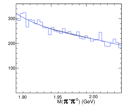
Figure 10: The invariant $\pi^{+}\pi^{0}$ mass. The curves are fits to a background polynomial and Gaussian signal with a width fixed by Monte Carlo simulation.

For the $\tau^{+}\nu$, $\tau^{+}\to\pi^{+}\overline{\nu}$ final state the real $D_{s}^{+}$ backgrounds include, in addition to the $\pi^{+}\pi^{0}$ background discussed above, semileptonic decays, possible $\pi^{+}\pi^{0}\pi^{0}$ decays and other $\tau^{+}$ decays. Semileptonic decays involving muons are equal to those involving electrons shown in Fig. 9(c). Since no electron events appear the signal region, the background from muons is also consistent with zero. The $\pi^{+}\pi^{0}\pi^{0}$ background is estimated by considering the $\pi^{+}\pi^{+}\pi^{-}$ final state whose measured branching ratio is (1.02$\pm$0.12)% stone-fpcp . This mode has large contributions from $f_{0}(980)\pi^{+}$ and other resonant structures in $\pi^{+}\pi^{-}$ at higher mass focus-3pi . The $\pi^{+}\pi^{0}\pi^{0}$ mode will also have these contributions, but the MM² opposite to the $\pi^{+}$ will be at large mass. The only component that can potentially cause background for us is the non-resonant part measured by FOCUS as (17$\pm$4)%. This background has been evaluated by Monte Carlo simulation as well as others from other $\tau^{+}$ decays, and listed in Table 2.

Table 2: Backgrounds in the $D_{s}^{+}\to\tau^{+}\nu$, $\tau^{+}\to\pi^{+}\overline{\nu}$ sample, case (i) for 0.2$>$MM${}^{2}>0.05$ GeV² and case (ii) for 0.2$>$MM${}^{2}>-0.05$ GeV²

Mode	${\cal{B}}$(%)	# of events case(i)	# of events case(ii)	Sum
$\pi^{+}\pi^{0}\pi^{0}$	1.0	0.1	0.3	0.4
$D_{s}^{+}\to\tau^{+}\nu$	6.2
$\tau^{+}\to\pi^{+}\pi^{0}\nu$	1.6	0.3	0.4	0.7
$\tau^{+}\to\mu^{+}\overline{\nu}\nu$	1.1	0	0	0
$\tau^{+}\to e^{+}\overline{\nu}\nu$	1.1	0.2	0	0.2
Sum		0.6	0.7	1.3

IV Checks of the Method

We perform an overall check of our procedures by measuring ${\cal{B}}(D_{s}^{+}\to\overline{K}^{0}K^{+})$. For this measurement we compute the MM² (Eq. 5) using events with an additional charged track but here identified as a kaon. These track candidates have momenta of approximately 1 GeV/c; here our RICH detector has a pion to kaon fake rate of 1.1% with a kaon detection efficiency of 88.5% fakes . For this study, we do not veto events with extra charged tracks or photons.

The MM² distribution is shown in Fig. 7. The peak near 0.25 GeV² is due to the decay mode of interest. We fit this to a linear background from 0.02-0.50 GeV² plus a two-Gaussian signal function. The fit yields 228$\pm$18$\pm$8 events. Since $\eta K^{+}$ could in principle contribute an asymmetric background in this region, we searched for this final state. Not finding any signal, we set an upper limit of 2.8$\times 10^{-3}$, approximately a factor of five below our measurement. In order to compute the branching fraction we must include the efficiency of detecting the kaon track 76.2%, including radiation gammamunu , and take into account that it is easier to detect the photon from the $D_{s}^{*}$ decay in $\overline{K}^{0}K^{+}$ events than in the average $D_{s}D_{s}^{*}$ event due to the track and photon multiplicities, which gives a 4% correction. These rates are estimated by using Monte Carlo simulation. We determine

$${\cal{B}}(D_{s}^{+}\to\overline{K}^{0}K^{+})=(2.74\pm 0.23\pm 0.13)\%,$$ (7)

where the systematic errors are listed in Table 3. The largest components of the systematic errors arise from the number of signal events (4.2%) from the signal function width (3%) and the shape of the background function (3%). This method is in good agreement with the latest double tag result Peter .

Table 3: Systematic errors on determination of the $D_{s}^{+}\to\overline{K}^{0}K^{+}$ branching ratio.

Error Source	Size (%)
Signal shape	1
Background shape	1
Track finding	0.7
PID cut	1.0
Number of tags	4.2
Total	4.6

V Leptonic Branching Fractions

The sum of MM² distributions for case (i) and case (ii) normalized to the expectation of the sum of $D_{s}^{+}\to\mu^{+}\nu$ and $D_{s}^{+}\to\tau^{+}\nu$, $\tau^{+}\to\pi^{+}\nu$ is shown in Fig. 11. The data are consistent with our expectation containing mostly signal for MM${}^{2}<$0.2 GeV². Recall there are 100 total events only 5.5 of which we estimate are background. Above 0.2 GeV² other, larger backgrounds enter.

Figure 11: The sum of case (i) and case (ii) MM² distributions compared to the predicted shapes for $D_{s}^{+}\to\mu^{+}\nu$ + $\tau^{+}\nu$, $\tau^{+}\to\pi^{+}\nu$.

The number of $\mu^{+}\nu$ events in the signal region, $N_{\mu\nu}$, is related to the number of tags, $N_{\rm tag}$ the branching ratios and the estimated backgrounds $N_{\rm bkgrd}$ as

$$N_{\mu\nu}-N_{\rm bkgrd}=N_{\rm tag}\cdot\epsilon\left[\epsilon^{\prime}{\cal{B}}(D_{s}^{+}\to\mu^{+}\nu)+\epsilon^{\prime\prime}{\cal{B}}(D_{s}^{+}\to\tau^{+}\nu;~{}\tau^{+}\to\pi^{+}\nu)\right],$$ (8)

where $\epsilon$ (79.5%) includes the efficiency for reconstructing the single charged track including final state radiation (77.8%), the (98.3$\pm$0.2)% efficiency of not having another unmatched cluster in the event with energy greater than 300 MeV, and for the fact that it is easier to find tags in $\mu^{+}\nu$ events than in generic decays by 4%, as determined by Monte Carlo simulation. The efficiency labeled $\epsilon^{\prime}$ is a product of the 99% muon efficiency for depositing less than 300 MeV in the calorimeter and 92.3% acceptance of the MM² cut of $|$MM${}^{2}<0.05|$. The quantity $\epsilon^{\prime\prime}$ is the fraction of $\tau^{+}\nu;~{}\tau^{+}\to\pi^{+}\nu$ events contained in the $\mu^{+}\nu$ signal window (13.2%) times the 60% acceptance for a pion to deposit less than 300 MeV/c in the calorimeter (6.4%).

The two $D_{s}^{+}$ branching ratios in Eq. 8 are related as

$${\cal{B}}(D_{s}^{+}\to\tau^{+}\nu;~{}\tau^{+}\to\pi^{+}\nu)=R\cdot{\cal{B}}(\tau^{+}\to\pi^{+}\nu){\cal{B}}(D_{s}^{+}\to\mu^{+}\nu)=1.076\cdot{\cal{B}}(D_{s}^{+}\to\mu^{+}\nu)~{},$$ (9)

where we take the Standard Model ratio for $R$ as given in Eq. 2 and ${\cal{B}}(\tau^{+}\to\pi^{+}\nu)$=11.06% PDG . This allows us to solve Eq. 8. Since $N_{\mu\nu}$= 64, $N_{\rm bkgrd}$=2, and $N_{tag}=11880\pm 399\pm 499$, we find

$${\cal{B}}(D_{s}^{+}\to\mu^{+}\nu)=(0.657\pm 0.090\pm 0.028)\%.$$ (10)

We can also sum the $\mu^{+}\nu$ and $\tau^{+}\nu$ contributions, where we restrict ourselves to the MM² region below 0.20 GeV². Eq. 8 still applies. The number of signal and background events changes to 100 and 7.4, respectively. The efficiency $\epsilon^{\prime}$ becomes unity, and $\epsilon^{\prime\prime}$ increases to 45.2%. Using this method, we find

$${\cal{B}}(D_{s}^{+}\to\mu^{+}\nu)=(0.664\pm 0.076\pm 0.028)\%.$$ (11)

The systematic errors on these branching ratios are given in Table 4.

Table 4: Systematic errors on determination of the $D_{s}^{+}\to\mu^{+}\nu$ branching ratio.

Error Source	Size (%)
Track finding	0.7
Photon veto	2
Minimum ionization	1
Number of tags	4.2
Total	5.2

We also can analyze the $\tau^{+}\nu$ final state independently. We use different MM² regions for cases (i) and (ii) defined above. For case (i) we define the signal region to be the interval 0.20$>$MM${}^{2}>$0.05 GeV², while for case (ii) we define the signal region to be the interval 0.20$>$MM${}^{2}>$-0.05 GeV². Case (i) includes 98% of the $\mu^{+}\nu$ signal, so we must exclude the region close to zero MM², while for case (ii) we are specifically selecting pions so the signal region can be larger. The upper limit on MM² is chosen to avoid background from the tail of the $\overline{K}^{0}\pi^{+}$ peak. The fractions of the MM² range accepted are 32% and 45% for case (i) and (ii), respectively.

We find 24 signal and 3.1 background events for case (i) and 12 signal and 1.7 backgrounds for case (ii). The branching ratio, averaging the two cases is

$${\cal{B}}(D_{s}^{+}\to\tau^{+}\nu)=(7.1\pm 1.4\pm 0.3)\%.$$ (12)

Lepton universality in the Standard Model requires that the ratio $R$ from Eq. 2 be equal to a value of 9.72. We measure

$$R\equiv\frac{\Gamma(D_{s}^{+}\to\tau^{+}\nu)}{\Gamma(D_{s}^{+}\to\mu^{+}\nu)}=10.8\pm 2.6\pm 0.2~{}.$$ (13)

Thus we see no deviation from the predicted value. Current results on $D^{+}$ leptonic decays also show no deviations ourDptotaunu . The absence of any detected electrons opposite to our tags allows us to set an upper limit of

$${\cal{B}}(D_{s}^{+}\to e^{+}\nu)=3.1\times 10^{-4}$$ (14)

at 90% confidence level; this is also consistent with Standard Model predictions and lepton universality.

Using our most precise value for ${\cal{B}}(D_{s}^{+}\to\mu^{+}\nu)$ from Eq. 11, that is derived using both our $\mu^{+}\nu$ and $\tau^{+}\nu$ samples, and Eq. 1, we extract

$$f_{D_{s}}=282\pm 16\pm 7{~{}\rm MeV}.$$ (15)

We combine with our previous result our-fDp

$$f_{D}^{+}=222.6\pm 16.7^{+2.8}_{-3.4}{\rm~{}MeV.}$$ (16)

and find a preliminary value for

$${\frac{f_{D_{s}^{+}}}{f_{D^{+}}}=1.27\pm 0.12\pm 0.03},$$ (17)

where a small part of the systematic cancels in our two measurements.

VI Conclusions

Theoretical models that predict $f_{D_{s}^{+}}$ and the ratio $\frac{f_{D_{s}^{+}}}{f_{D^{+}}}$ are listed in Table 5. Our result is higher than most theoretical expectations. We are consistent with Lattice-Gauge theory, and most other models, for the ratio of decay constants.

Table 5: Theoretical predictions of $f_{D^{+}}$ and $f_{D_{S}^{+}}/f_{D^{+}}$. QL indicates quenched lattice calculations.

Model	$f_{D_{s}^{+}}$ (MeV)	$f_{D^{+}}$ (MeV)	$f_{D_{s}^{+}}/f_{D^{+}}$
Lattice ($n_{f}$=2+1) Lat:Milc	$249\pm 3\pm 16$	$201\pm 3\pm 17$	$1.24\pm 0.01\pm 0.07$
QL (Taiwan) Lat:Taiwan	$266\pm 10\pm 18$	$235\pm 8\pm 14$	$1.13\pm 0.03\pm 0.05$
QL (UKQCD) Lat:UKQCD	$236\pm 8^{+17}_{-14}$	$210\pm 10^{+17}_{-16}$	$1.13\pm 0.02^{+0.04}_{-0.02}$
QL Lat:Damir	$231\pm 12^{+6}_{-1}$	$211\pm 14^{+2}_{-12}$	$1.10\pm 0.02$
QCD Sum Rules Bordes	$205\pm 22$	$177\pm 21$	$1.16\pm 0.01\pm 0.03$
QCD Sum Rules Chiral	$235\pm 24$	$203\pm 20$	$1.15\pm 0.04$
Quark Model Quarkmodel	268	$234$	1.15
Quark Model QMII	248$\pm$27	$230\pm$25	1.08$\pm$0.01
Potential Model Equations	241	238	1.01
Isospin Splittings Isospin		$262\pm 29$

By using a theoretical prediction for $f_{D_{s}^{+}}/f_{D^{+}}$ we can derive a value for the ratio of CKM elements $|V_{cd}/V_{cs}|$. Taking the value from Ref. Lat:Milc of $1.24\pm 0.01\pm 0.07$, we find

$$|V_{cd}/V_{cs}|=0.22\pm 0.03~{},$$ (18)

where the theoretical and experimental errors have been added in quadrature. This value is consistent with expectations.

We now compare our preliminary results with previous measurements. The branching fractions modes and derived values of $f_{D_{s}^{+}}$ are listed in Table 6. Our values are shown first. We are generally consistent with previous measurements that are also higher than the theory.

Table 6: These results compared with previous measurements. Results have been updated for new values of the $D_{s}$ lifetime. ALEPH uses both measurements to derive a value for the decay constant.

Exp.	Mode	${\cal{B}}$	${\cal{B}}_{\phi\pi}$ (%)	$f_{D_{s}^{+}}$ (MeV)
CLEO-c	$\mu^{+}\nu$	$(6.57\pm 0.90\pm 0.34)10^{-3}$		$281\pm 19\pm 7$
CLEO-c	$\tau^{+}\nu$	$(7.1\pm 1.4\pm 0.3)10^{-2}$		$296\pm 29\pm 7$
CLEO-c	combined	-		$282\pm 16\pm 7$
CLEO CLEO	$\mu^{+}\nu$	$(6.2\pm 0.8\pm 1.3\pm 1.6)10^{-3}$	3.6$\pm$0.9	$273\pm 19\pm 27\pm 33$
BEATRICE BEAT	$\mu^{+}\nu$	$(8.3\pm 2.3\pm 0.6\pm 2.1)10^{-3}$	3.6$\pm$0.9	$315\pm 43\pm 12\pm 39$
ALEPH ALEPH	$\mu^{+}\nu$	$(6.8\pm 1.1\pm 1.8)10^{-3}$	3.6$\pm$0.9	$285\pm 19\pm 40$
ALEPH ALEPH	$\tau^{+}\nu$	$(5.8\pm 0.8\pm 1.8)10^{-2}$
OPAL OPAL	$\tau^{+}\nu$	$(7.0\pm 2.1\pm 2.0)10^{-3}$		$286\pm 44\pm 41$
L3 L3	$\tau^{+}\nu$	$(7.4\pm 2.8\pm 1.6\pm 1.8)10^{-3}$		$302\pm 57\pm 32\pm 37$
BaBar Babar-munu	$\mu^{+}\nu$	$(6.5\pm 0.8\pm 0.3\pm 0.9)10^{-3}$	4.8$\pm$0.5$\pm$0.4	$279\pm 17\pm 6\pm 19$

Most measurements of $D_{s}^{+}\to\ell^{+}\nu$ are normalized with respect to ${\cal{B}}(D_{s}^{+}\to\phi\pi^{+})$. One measurement that isn’t is that of OPAL, which normalizes to a $D_{s}$ fraction in $Z^{0}$ events that is derived from an overall fit to heavy flavor data at LEP HFAG . It still, however, relies on absolute branching fractions that are hidden by this procedure, and the estimated error on the normalization is somewhat smaller than that indicated by the error on ${\cal{B}}_{\phi\pi}$ available at the time of their publication. The L3 measurement is normalized to using a calculation that the fraction of $D_{s}$ mesons produced in $c$ quark fragmentation is 0.11$\pm$0.02 and that ratio of $D_{s}^{*}/D_{s}$ production is 0.65$\pm$0.10. The ALEPH results use ${\cal{B}}_{\phi\pi}$ for their $\mu^{+}\nu$ results and a similar procedure as OPAL for their $\tau^{+}\nu$ results. We note that the recent BaBar result uses a larger ${\cal{B}}_{\phi\pi}$ than the other results.

The CLEO-c determination of $f_{D_{s}^{+}}$ is the most accurate to date. It also does not rely on the independent determination of any normalization mode.

VII Acknowledgments

We gratefully acknowledge the effort of the CESR staff in providing us with excellent luminosity and running conditions. This work was supported by the National Science Foundation, the U.S. Department of Energy, and the Natural Sciences and Engineering Research Council of Canada.

References

- (1) G. Buchalla, A. J. Buras and M. E. Lautenbacher, Rev. Mod. Phys. 68, 1125 (1996) [hep-ph/9512380].
- (2) G. Gomez-Ceballos, “Update on CDF Mixing,” invited talk presented at Flavor Physics and CP Violation, April 6-12, 2006, Vancouver Canada (http://fpcp2006.triumf.ca/agenda.php). See also V. Abazov et al. (D0), “First Direct Two-Sided Bound on the Oscillation Frequency,” (2006) [hep-ex/0603029].
- (3) S. Eidelman et al. (PDG), Phys. Lett. B 592, 1 (2004).
- (4) A recent measurement of the decay rate for measures the product of , but does not provide an accurate value of , because of its inherent imprecision and also because of the relative large error on . See K. Ikado et al. (Belle), “Evidence of the Purely Leptonic Decay [hep-ex/0604018].
- (5) C. Davies et al., Phys. Rev. Lett. 92, 022001 (2004).
- (6) M. Artuso et al. (CLEO Collaboration), Phys. Rev. Lett. 95, 251801 (2005) [hep-ex/0508057].
- (7) G. Bonvicini, et al. (CLEO) Phys. Rev. D70, 112004 (2004) [hep-ex/0411050].
- (8) D. Silverman and H. Yao, Phys. Rev. D 38, 214 (1988).
- (9) S. Stone, “Hadronic Charm Decays and Mixing,” inivted talk at Flavor Physics and CP Violation Conference, Vancouver, 2006 [hep-ph/0605134].
- (10) D. Peterson et al., Nucl. Instrum. and Meth. A478, 142 (2002); M. Artuso et al., Nucl. Instrum. and Meth. A502, 91 (2003); Y. Kubota et al. (CLEO Collaboration), Nucl. Instrum. and Meth. A320, 66 (1992).
- (11) Private communication from R. Sia.
- (12) R. Poling, “CLEO-c Hot Topics,” presented at Flavor Physics and CP Violation, April 9-12, 2006, Vancouver, B. C., Canada.
- (13) T. Skwarnicki, “A Study of the Radiative Cascade Transitions Between the Upsilon-Prime and Upsilon Resonances,” DESY F31-86-02 (thesis, unpublished) (1986).
- (14) P. Rubin et al. (CLEO), Phys. Rev. D73, 112005 (2006) [hep-ex/0604043].
- (15) S. Malvezzi (FOCUS), “Dalitz Plot Analysis in the FOCUS Experiment,” J. Phys. Conf. Ser. 9, 165 (2005).
- (16) M. Artuso et al., Nucl. Instrum. Meth. A554, 147 (2005) [physics/0506132].
- (17) E. Barberio, B. van Eijk, Z. Was, Comput. Phys. Commun. 66, 115 (1991); E. Barberio and Z. Wa̧s, Comput. Phys. Commun. 79, 291 (1994).
- (18) The most recent value for is (1.500.08)%, which when doubled gives (3.000.16)%. Private communication from Peter Onyisi.
- (19) P. Rubin et al. (CLEO), Phys. Rev. D73, 112005 (2006).
- (20) C. Aubin et al., Phys. Rev. Lett. 95, 122002 (2005).
- (21) T. W. Chiu et al., Phys. Lett. B624, 31 (2005)[hep-ph/0506266].
- (22) L. Lellouch and C.-J. Lin (UKQCD), Phys. Rev. D 64, 094501 (2001).
- (23) D. Becirevic et al., Phys. Rev. D 60, 074501 (1999).
- (24) J. Bordes, J. Peñarrocha, and K. Schilcher, “ and Decay Constants from QCD Duality at Three Loops,” [hep-ph/0507241].
- (25) S. Narison, “Light and Heavy Quark Masses, Flavour Breaking of Chiral Condensates, Meson Weak Leptonic Decay Constants in QCD,” [hep-ph/0202200] (2002).
- (26) D. Ebert et al., Phys. Lett. B635, 93 (2006).
- (27) G. Cvetič et al., Phys. Lett. B596, 84 (2004).
- (28) Z. G. Wang et al., Nucl. Phys. A744, 156 (2004); L. Salcedo et al., Braz. J. Phys. 34, 297 (2004).
- (29) J. Amundson et al., Phys. Rev. D 47, 3059 (1993).
- (30) M. Chadha et al. (CLEO), Phys. Rev. D58, 032002 (1998).
- (31) Y. Alexandrov et al. (BEATRICE), Phys. Lett. B478, 31 (2000).
- (32) A. Heister et al. (ALEPH) Phys. Lett. B528, 1 (2002) [hep-ex/0201024].
- (33) M. Acciarri et al. (L3), Phys. Lett. B396, 327 (1997).
- (34) G. Abbiendi et al. (OPAL), Phys. Lett. B516, 236 (2001).
- (35) ALEPH, DELPHI, L3, and OPAL Collaborations, Nucl. Instr. and Meth. A378, 101 (1996).
- (36) J. Berryhill, “New results from BaBar: Rare Meson Decays and the Search for New Phenomena,” presented at XLIst Rencontres de Moriond: Electroweak Interactions and Unified Theories [http://moriond.in2p3.fr/EW/2006/Transparencies/J.W.Berryhill.pdf].