$\chi_{cJ}$ Decays to $h^{+}h^{-}h^{0}$  

Abstract

Using a sample of $3\times 10^{6}$ $\psi(2S)$ decays recorded by the CLEO detector, we study three body decays of the $\chi_{c0}$, $\chi_{c1}$, and $\chi_{c2}$ produced in radiative decays of the $\psi(2S)$. We consider the decay modes $\pi^{+}\pi^{-}\eta$, $K^{+}K^{-}\eta$, $p{\bar{p}}\eta$, $\pi^{+}\pi^{-}\eta^{\prime}$, $K^{+}K^{-}\pi^{0}$, $p{\bar{p}}\pi^{0}$, $\pi^{+}K^{-}K^{0}_{\rm S}$, and $K^{+}{\bar{p}}\Lambda$ measuring branching fractions or placing upper limits. For $\chi_{c1}\to\pi^{+}\pi^{-}\eta$, $K^{+}K^{-}\pi^{0}$, and $\pi^{+}K^{-}K^{0}_{\rm S}$ our observed samples are large enough to study the substructure in a Dalitz plot analysis. The results presented in this document are preliminary.

Decays of the $\chi_{cJ}$ states are not as well studied both experimentally and theoretically as those of other charmonium states. It is possible that the color-octet mechanism, $c\bar{c}g\to 2(q\bar{q})$ could have large effects on the observed decay pattern of the $\chi_{cJ}$ states quarkoniumreview . Thus any knowledge of any hadronic decay channels for these state is valuable.

CLEO has gathered a large sample of $e^{+}e^{-}\to\psi(2S)$ which leads to copious production of the $\chi_{cJ}$ states in radiative decays of the $\psi(2S)$. This contribution describes our study of selected three body hadronic decay modes of the $\chi_{cJ}$ to two charged and one neutral hadron. This is not an exhaustive study of $\chi_{cJ}$ hadronic decays; we do not even comprehensively cover all possible $h^{+}h^{-}h^{0}$ decays, but simply take a first look at the rich structure of $\chi_{cJ}$ decays in our initial $\psi(2S)$ data sets. With the CLEO III detector configuration CLEOIII , we have observed an integrated luminosity of 2.57 pb^-1 and the number of $\psi(2S)$ events is $1.56\times 10^{6}$. With the CLEO-c detector configuration CLEOc we have observed 2.89 pb^-1, and the number of events is $1.52\times 10^{6}$. Note that the apparent mis-match of luminosities and event totals is due to different beam energy spreads for the two data sets.

Our basic technique is an exclusive whole event analysis. A photon candidate is combined with three hadrons and the 4-momentum sum constrained to the known beam energy and small beam momentum caused by the beam crossing angle taking into account the measured errors on the reconstructed charged tracks, neutral hadron, and transition photon. We cut on the $\chi^{2}$ of this fit, which has four degrees of freedom, as it strongly discriminates between background and signal. Efficiencies and backgrounds are studied in a GEANT-based simulation cleog of the detector response to underlying $e^{+}e^{-}\to\psi(2S)$ events. Our simulated sample is roughly ten times our data sample. The simulation is generated with a $1+\lambda\cos^{2}\theta$ distribution in $\cos\theta$, where $\theta$ is the radiated photon angle relative to the positron beam axis. A E1 transition, as expected for $\psi(2S)\to\gamma\chi_{cJ}$, implies $\lambda=1,-1/3,+1/13$ for $J=0,1,2$ particles. The efficiencies we quote use this simulation. The differences of efficiencies due to various $\theta$ distributions are negligible as we accept transition photons down to our detection limit.

A kinematic fit is made to each event. For most modes we select events with an event 4-momentum fit $\chi^{2}$ less than 25, but background from $\psi(2S)\to J/\psi\pi^{0}\pi^{0}$ followed by charged two body decays of the $J/\psi$ with one of the $\pi^{0}$ decay photons lost fakes $\psi(2S)\to\gamma\chi_{cJ}\to\gamma p{\bar{p}}\pi^{0}$. For this mode the cut on $\chi^{2}$ is tightened to 12. The efficiency of this cut is $\approx$ 95% for all modes except $p{\bar{p}}\pi^{0}$ where it is $\approx$ 80%. Little background survives.

Photon candidates are energy depositions in our crystal calorimeter that have a transverse shape consistent with that expected for an electromagnetic shower without a charged track pointing toward it. They have an energy of at least 30 MeV. Transition photon candidates are vetoed if they form a $\pi^{0}$ or $\eta$ candidate when paired with a second photon candidate. Photon candidates that are formed into neutral particles further must have an energy of more than 50 MeV if they are not in the central barrel of our calorimeter. $\pi^{0}\to\gamma\gamma$ and $\eta\to\gamma\gamma$ candidates are formed from two photon candidates that are kinematically fit to the known resonance masses using the event vertex position, determined using charged tracks constrained to the beam spot. We select those giving a $\chi^{2}$ from the kinematic mass fit with one degree of freedom of less than 10.

We also select the $\eta\to\pi^{+}\pi^{-}\pi^{0}$ mode combining two charged pions with a $\pi^{0}$ candidate increasing the efficiency for $\eta$ reconstruction by about 25%. The same sort of kinematic mass fit as used for $\pi^{0}$’s and $\eta\to\gamma\gamma$ is applied to this mode, and again we select those giving a $\chi^{2}$ of less than 10. Similarly we combine the mass-constrained $\eta$’s together with two charged pions to make $\eta^{\prime}$ candidates, mass constrain them, and select those with $\chi^{2}<10$. In addition, we include the decay mode $\eta^{\prime}\to\gamma\rho$. Here the background is potentially high because of the large number of noise photons, so we require $E_{\rm photon}>200$ MeV. In addition, we require the $\pi^{+}\pi^{-}$ mass to be within 100 MeV/c² of the $\rho$ mass.

Charged tracks have standard requirements that they be of good fit quality. Those coming from the origin must have an impact parameter with respect to the beam spot less than the maximum of $(5.0-(3.8\cdot p))$ mm or 1.2 mm, where $p$ is the measured track momentum in GeV/c. $K^{0}_{S}\to\pi^{+}\pi^{-}$ and $\Lambda\to p\pi^{-}$ candidates are formed from good quality tracks that are constrained to come from a common vertex. The $K^{0}_{S}$ flight path is required to be greater than 5 mm and the $\Lambda$ flight path greater than 3 mm. The mass cut around the $K^{0}_{S}$ mass is $\pm 10$ MeV/c², and around the $\Lambda$ mass $\pm 5$ MeV/c². Events with only the exact number of selected tracks are accepted. This selection is very efficient, $>$99.9%, for events passing all other requirements.

Pions are required to have specific ionization, $dE/dx$, in our main drift chamber within four standard deviations of the expected value for a real pion at the measured momentum. For kaons and protons, a combined $dE/dx$ and RICH likelihood is formed and kaons are simply required to be more kaon-like than pion or proton-like, and similarly for protons. Cross feed between hadron species is negligible after all other requirements.

In modes comprising only two charged particles, there are some extra cuts to eliminate QED background which produce charged leptons in the final state. Events are rejected if the sum over all the charged tracks produces a penetration into the muon system of more than five interaction lengths. Events are rejected if any track has $0.92<E/p<1.05$ and it has a $dE/dx$ consistent with an electron. This latter cut is not used for $p\bar{p}$ modes because anti-protons tend to deposit all their energy in the calorimeter. These cuts are essentially 100% efficient for the signal, and do eliminate the small QED background.

The efficiencies averaged over the CLEO III and CLEO-c data sets for each mode including the branching fractions $\eta\to\gamma\gamma$, $\eta\to\pi^{+}\pi^{-}\pi^{0}$, and $\eta^{\prime}\to\eta\pi^{+}\pi^{-}$ are given in Tables 1-3 for $\chi_{c0}$, $\chi_{c1}$, and $\chi_{c2}$ respectively.

Figure 1: Mass distribution for candidate $\chi_{cJ}\to\pi^{+}\pi^{-}\eta$. The displayed fit is described in the text.

Figure 2: Mass distribution for candidate $\chi_{cJ}\to K^{+}K^{-}\eta$. The displayed fit is described in the text.

Figure 3: Mass distribution for candidate $\chi_{cJ}\to p{\bar{p}}\eta$. The displayed fit is described in the text.

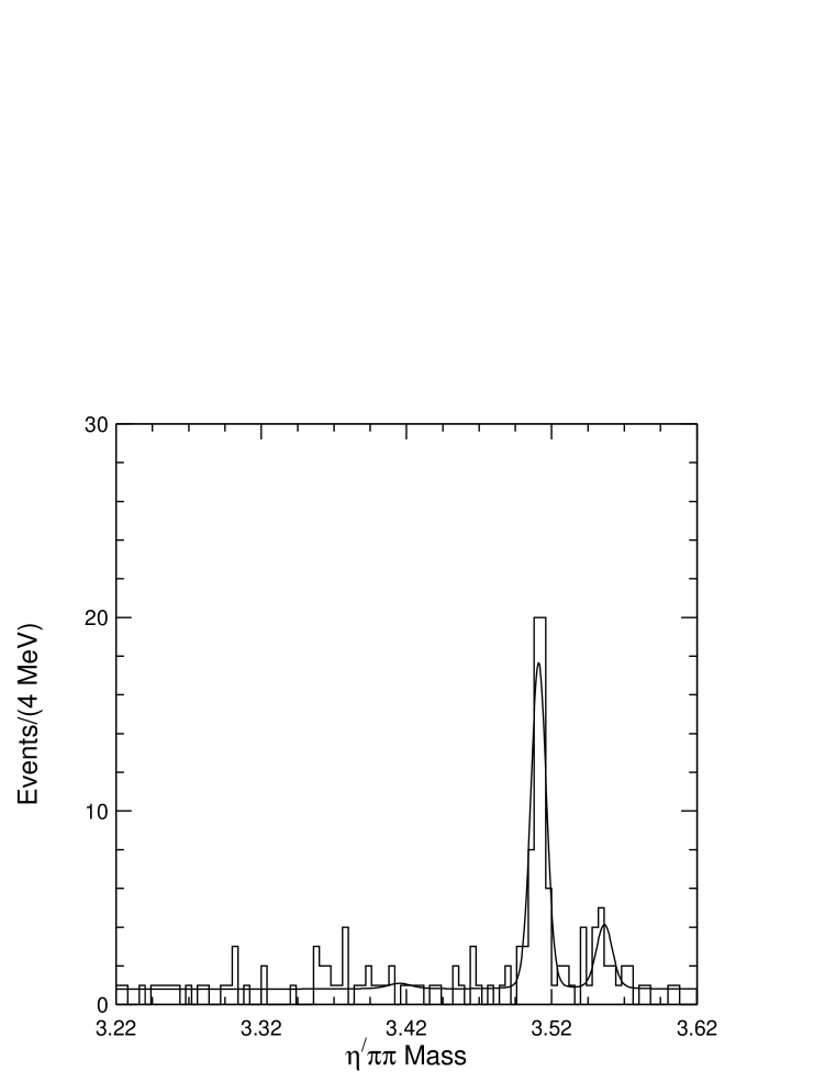
Figure 4: Mass distribution for candidate $\chi_{cJ}\to\pi^{+}\pi^{-}\eta^{\prime}$. The displayed fit is described in the text.

Figure 5: Mass distribution for candidate $\chi_{cJ}\to K^{+}K^{-}\pi^{0}$. The displayed fit is described in the text.

Figure 6: Mass distribution for candidate $\chi_{cJ}\to p{\bar{p}}\pi^{0}$. The displayed fit is described in the text.

Figure 7: Mass distribution for candidate $\chi_{cJ}\to K^{0}_{\rm S}K^{-}\pi^{+}$. The displayed fit is described in the text.

Figure 8: Mass distribution for candidate $\chi_{cJ}\to K^{+}{\bar{p}}\Lambda$. The displayed fit is described in the text.

Figures 1-8 show the mass distributions for the eight $\chi_{cJ}$ decay modes selected by the analysis described above. Signals are evident in all three $\chi_{cJ}$ states, but not in all the modes. Backgrounds are small. The mass distributions are fit to three signal shapes, Breit-Wigners convolved with Gaussian detector resolutions, and a linear background. The $\chi_{cJ}$ masses and intrinsic widths are fixed at the values from the Particle Data Group compilation pdg . The detector resolution is taken from the simulation discussed above. The simulation properly takes into account the amount of data in the two detector configurations, and the distribution of different decay modes we have observed. We approximate the resolution with a single Gaussian distribution, and variations are considered in the determination of systematic uncertainty. The detector resolution dominates for the $\chi_{c1}$ and $\chi_{c2}$, but is similar to the intrinsic width of the $\chi_{c0}$. The fits are displayed in Figures 1-8 and summarized in Tables 1-3.

Table 1: Parameters used and results of fits to the $\chi_{cJ}$ mass distributions of Figures 1-8 for the $\chi_{c0}$ signal. The fit is described in the text and the yield error is only statistical. If no significant signal is observed the 90% confidence level limit is also shown.

Mode	Efficiency (%)	Resolution (MeV)	Yield
$\pi^{+}\pi^{-}\eta$	17.6	6.23	$4.0\pm 4.1$ ($<10.6$)
$K^{+}K^{-}\eta$	13.6	6.10	$3.1\pm 2.7$ ($<9.3$)
$p{\bar{p}}\eta$	15.8	5.42	$17.7^{+5.2}_{-4.8}$
$\pi^{+}\pi^{-}\eta^{\prime}$	7.8	4.38	$1.8\pm 3.8$ ($<8.5$)
$K^{+}K^{-}\pi^{0}$	26.4	6.47	$-3.3\pm 2.7$ ($<4.7$)
$p{\bar{p}}\pi^{0}$	27.1	5.80	$46.2^{+8.0}_{-7.2}$
$\pi^{+}K^{-}K^{0}_{\rm S}$	19.0	4.75	$0.0\pm 1.0$ ($<2.7$)
$K^{+}{\bar{p}}\Lambda$	16.7	4.38	$51.2^{+8.1}_{-7.4}$

Table 2: Parameters used and results of fits to the $\chi_{cJ}$ mass distributions of Figures 1-8 for the $\chi_{c1}$ signal. The fit is described in the text and the yield error is only statistical. If no significant signal is observed the 90% confidence level limit is also shown.

Mode	Efficiency (%)	Resolution (MeV)	Yield
$\pi^{+}\pi^{-}\eta$	18.1	5.85	$255^{+17}_{-16}$
$K^{+}K^{-}\eta$	14.2	5.66	$14.1^{+4.6}_{-3.9}$
$p{\bar{p}}\eta$	17.6	5.41	$3.2\pm 2.3$ ($<7.6$)
$\pi^{+}\pi^{-}\eta^{\prime}$	8.3	4.37	$57.6^{+8.4}_{-7.7}$
$K^{+}K^{-}\pi^{0}$	28.2	6.79	$157\pm 13$
$p{\bar{p}}\pi^{0}$	29.5	5.23	$9.9^{+3.8}_{-3.2}$
$\pi^{+}K^{-}K^{0}_{\rm S}$	19.8	4.37	$249\pm 16$
$K^{+}{\bar{p}}\Lambda$	17.5	4.38	$16.3^{+4.7}_{-4.0}$

Table 3: Parameters used and results of fits to the $\chi_{cJ}$ mass distributions of Figures 1-8 for the $\chi_{c2}$ signal. The fit is described in the text and the yield error is only statistical. If no significant signal is observed the 90% confidence level limit is also shown.

Mode	Efficiency (%)	Resolution (MeV)	Yield
$\pi^{+}\pi^{-}\eta$	17.8	5.58	$26.2^{+6.4}_{-5.7}$
$K^{+}K^{-}\eta$	14.1	5.53	$6.9\pm 2.9$ ($<12.54$)
$p{\bar{p}}\eta$	16.9	5.08	$9.5^{+3.8}_{-3.0}$
$\pi^{+}\pi^{-}\eta^{\prime}$	8.2	4.32	$12.4^{+4.8}_{-4.1}$
$K^{+}K^{-}\pi^{0}$	27.5	6.85	$24.8^{+5.8}_{-5.1}$
$p{\bar{p}}\pi^{0}$	28.9	5.10	$37.1^{+6.7}_{-6.1}$
$\pi^{+}K^{-}K^{0}_{\rm S}$	17.2	4.45	$36.8^{+6.6}_{-5.9}$
$K^{+}{\bar{p}}\Lambda$	17.5	4.32	$42.1^{+7.2}_{-6.5}$

Note that for the $\chi_{c0}$ in Table 1 the five modes for which no significant signal are found are forbidden by parity conservation.

We consider various sources of systematic uncertainties on the yields. We varied the fitting procedure by allowing the $\chi_{cJ}$ masses and intrinsic widths to float. The fitted masses and widths agree with the fixed values from the particle data group, and we take the maximum variation in the observed yields, 4%, as a systematic uncertainty from the fit procedure. Allowing a curvature term to the background has a negligible effect. For modes with large yields we can break up the sample into CLEO III and CLEO-c data sets, and fit with resolutions and efficiencies appropriate for the individual data sets. We note that the separate data sets give consistent efficiency corrected yields and the summed yield differs by 2% from the standard procedure, which is small compared to the 8% statistical uncertainty. We take this as the systematic uncertainty from our resolution model. From studies of other processes we assign a 0.7% uncertainty for the efficiency of finding each charged track, 2.0% for the $\gamma\gamma$ resonances, 1.0% for each extra photon, 1.3% for the particle identification for each $K$ and $p$, 2.0% for secondary vertex finding, and 3.0% from the statistical uncertainty on the efficiency determined from the simulation. We study the cut on the $\chi^{2}$ of event 4-momentum kinematic fit in the three large yield $\chi_{c1}$ signals by removing the $\chi^{2}$ cut, selecting events around the $\chi_{c1}$ mass peak, subtracting a low mass side band, the only one available, and comparing the simulated $\chi^{2}$ distribution for signal events with the data distribution. This comparison is shown in Figure 9. The agreement

Figure 9: Distribution of the $\chi^{2}$ of the beam energy constrained mass fit. This is shown with a mass cut around the $\chi_{c1}$ signal region and after a data sideband subtraction. The plot on the left is for the $\pi^{+}\pi^{-}\eta$ mode, center is the $K^{+}K^{-}\pi^{0}$ mode, and right is the $\pi^{+}K^{-}K^{0}_{\rm S}$ mode. The data are shown by points and the simulation of signal events is shown by the histogram.

between the data and simulation is good, and comparing the inefficiency introduced by our cut on the 4-momentum kinematic fit $\chi^{2}$ between the data and the simulation we assign a 3.5% uncertainty on the efficiency due to uncertainty in modeling this $\chi^{2}$ distribution. The simulation was generated assuming 3-body phase-space for the $\chi_{cJ}$ decay products. Deviations from this are to be expected. Based on the results of the Dalitz plot analyses discussed below we correct the efficiency in the $\chi_{c1}\to\pi^{+}\pi^{-}\eta$, $\chi_{c1}\to K^{+}K^{-}\pi^{0}$, and $\chi_{c1}\to K^{-}\pi^{+}K^{0}_{S}$ modes by a relative $+6$% to account for the change in the efficiency caused by the deviation from a uniform phase space distribution of decay products to what we actually observe. This correction only has a noticeable impact on the $\chi_{c1}\to K^{-}\pi^{+}K^{0}_{S}$ mode.

To calculate $\chi_{cJ}$ branching fractions, we use previous CLEO measurements for the $\psi(2S)\to\chi_{cJ}$ branching fractions of $9.3\pm 0.14\pm 0.61$%, $9.07\pm.11\pm.54$% and $9.22\pm.11\pm.54$% for $J$=0,1,2 respectively chicbf . The uncertainties on these branching fractions are included in the systematic uncertainty on the $\chi_{cJ}$ branching fractions we report. Preliminary results for the three body branching fractions are shown in Table 4. Where the yields do not show clear signals

Table 4: Preliminary branching fractions in %. Uncertainties are statistical, systematic due to detector effects plus analysis methods and a separate systematic due to uncertainties in the $\psi(2S)$ branching fractions. Limits are at the 90% confidence level.

Mode	$\chi_{c0}$	$\chi_{c1}$	$\chi_{c2}$
$\pi^{+}\pi^{-}\eta$	$<0.021$	$0.52\pm.03\pm.03\pm.03$	$0.051\pm.011\pm.004\pm.003$
$K^{+}K^{-}\eta$	$<0.024$	$0.034\pm.010\pm.003\pm.002$	$<0.033$
$p\bar{p}\eta$	$0.038\pm.010\pm.003\pm.02$	$<0.015$	$.019\pm.007\pm.002\pm.002$
$\pi^{+}\pi^{-}\eta^{\prime}$	$<0.038$	$0.24\pm.03\pm.02\pm.02$	$<0.053$
$K^{+}K^{-}\pi^{0}$	$<0.006$	$0.200\pm.015\pm.018\pm.014$	$0.032\pm.007\pm.002\pm.002$
$p\bar{p}\pi^{0}$	$0.059\pm.010\pm.006\pm.004$	$0.014\pm 0.005\pm 0.001\pm 0.001$	$0.045\pm.007\pm 0.004\pm.003$
$\pi^{+}K^{-}{\bar{K}^{0}}$	$<0.010$	$0.84\pm.05\pm.06\pm.05$	$0.15\pm.02\pm.01\pm.01$
$K^{+}\bar{p}\Lambda$	$0.114\pm.016\pm.009\pm.007$	$0.034\pm.009\pm.003\pm.002$	$0.088\pm.014\pm.07\pm.006$

we calculate 90% confidence level upper limits using the yield central values with the statistical errors from the yield fits combined in quadrature with the systematic uncertainties on the efficiencies and other branching fractions. We assume the uncertainty is distributed as a Gaussian and the upper limit is the branching fraction value at which 90% of the integrated area of the Gaussian falls below. We exclude the unphysical region, negative branching fractions, for this upper limit calculation. We note that the ratio of rates expected from isospin symmetry, as discussed in Appendix I, Equations 15 and 23, expected to be 4.0 is consistent with our measurement:

$$\frac{\Gamma(\chi_{c1}\to\pi^{+}K^{-}K^{0})+\Gamma(\chi_{c1}\to\pi^{-}K^{+}\overline{K^{0}})}{\Gamma(\chi_{c1}\to\pi^{0}K^{+}K^{-})}=4.2\pm 0.7.$$ (1)

We choose the three high-statistics signals $\chi_{c1}\to\pi^{+}\pi^{-}\eta$, $\chi_{c1}\to K^{+}K^{-}\pi^{0}$, and $\chi_{c1}\to K^{-}\pi^{+}K^{0}_{S}$ for Dalitz plot analysis to study resonance substructure. For the Dalitz analysis only those events within 10 MeV, roughly two standard deviations, of the signal peak are accepted. For $\chi_{c1}\to\pi^{+}\pi^{-}\eta$ there are 228 events in this region and the signal fit finds 224.2 signal events and 5.1 combinatorial background. For $\chi_{c1}\to K^{+}K^{-}\pi^{0}$ there are 137 events accepted with the fit finding 137.8 signal and 2.4 background events, and for $\chi_{c1}\to K^{-}\pi^{+}K^{0}_{S}$, the numbers are 234 events, of which 233.2 are signal and 0.8 are background. In all cases the contribution from the tail of the $\chi_{c2}$ is less than one event.

An unbinned maximum likelihood fit is used along with other methods as described in cleodalitz in order to perform the Dalitz plot analysis. We only summarize our methods here. Efficiencies are determined with simulated event samples generated uniformly in phase space, and run through the analysis procedure described above. The efficiency across the Dalitz plots is fit to a two dimensional polynomial of third order in the Dalitz plot variables. The fits are of good quality and the efficiency is generally flat across the Dalitz plot.

When fitting the data Dalitz plot the small contributions from backgrounds are neglected. We use an isobar model to describe resonance contributions to the Dalitz plots taking into account spin and width dependent effects. Narrow resonances are described with a Breit-Wigner amplitude with the resonance parameters taken from previous experiments pdg . For the scalar resonances $a_{0}(980)$ and $f_{0}(980)$ we use a Flatté parameterization. We use the $a_{0}(980)$ line-shape from the Crystal Barrel Collaboration CBarrel_a0_980 and the details of the $f_{0}(980)$ are unimportant as it is used only in systematic studies. For low mass $\pi^{+}\pi^{-}$($\sigma$) and $K\pi$($\kappa$) S-wave contributions we choose a simple description, one which is adequate for our small sample Oller_2005 .

We are examining the $e^{+}e^{-}\to\psi(2S)\to\gamma\chi_{c1}$ process. In such a decay the $\chi_{c1}$ should be polarized. In principal a more complete analysis would take into account the angle of the photon with respect to the $e^{+}e^{-}$ beams collision axis and decompose the $\chi_{c1}$ decay into its partial waves. We barely have the statistics to do a reasonable Dalitz analysis suggesting that a higher dimensional partial wave analysis would be hopeless. See Appendix II for a discussion and the formalism of how polarization would affect the Dalitz analysis when the intermediate resonance is not spin zero even when integrated over the random polarization direction of the $\chi_{c1}$. Keeping this in mind, for this Dalitz plot analysis we decided to use angular distributions from Filippini-Fontana-Rotondi . We have tested different angular distributions and include the variations as a systematic uncertainty.

Figure 10 shows the Dalitz plot and three projections for $\chi_{c1}\to\pi^{+}\pi^{-}\eta$.

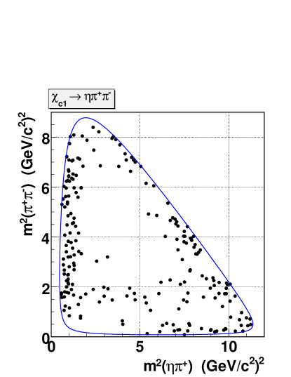
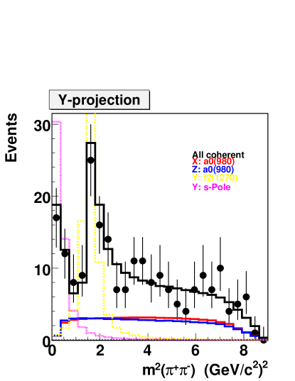
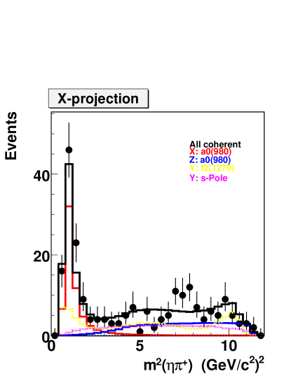
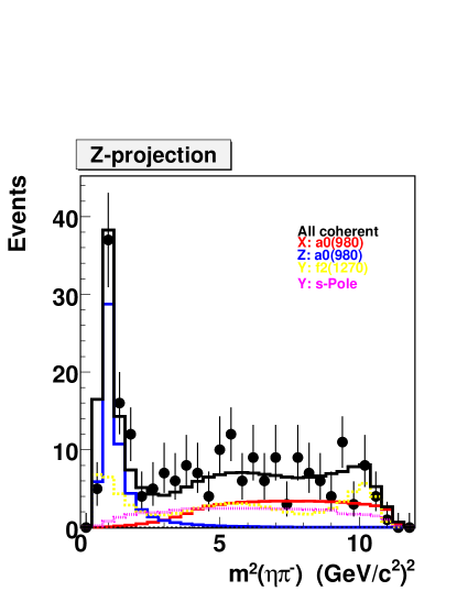
Figure 10: Dalitz plot and projections on the three mass squared combinations for $\chi_{c1}\to\pi^{+}\pi^{-}\eta$. The displayed fit projections are described in the text.

There are clear contributions from $a_{0}(980)^{\pm}\pi^{\mp}$ and $f_{2}(1270)\eta$ intermediate states, and significant accumulation at low $\pi^{+}\pi^{-}$ mass. Note that the $a_{0}(980)$ can contribute in two decay modes to the Dalitz plot. An isospin Clebsch-Gordan decomposition for this decay, given in Appendix I, Equation 16, shows that amplitudes and strong phases of both charge-conjugated states should be equal. The overall amplitude normalization and one phase are arbitrary parameters and we set $a_{a_{0}(980)^{+}}=a_{a_{0}(980)^{-}}=1$, $\phi_{a_{0}(980)^{+}}=\phi_{a_{0}(980)^{-}}=0$. All other fit components are defined with respect to these choices for $a_{0}(980)$.

Our initial fit to this mode includes only $a_{0}(980)^{\pm}\pi^{\mp}$ and $f_{2}(1270)\eta$ contributions, but has a low probability of describing the data, 0.13%, due to the accumulation of events at low $\pi^{+}\pi^{-}$ mass. To account for this we try $K^{0}_{S}$, $f_{0}(980)$, $\rho(770)$, and $\sigma$ resonances. Only the $\rho(770)$ and the $\sigma$ give high fit probability, 49% and 58% respectively. However the decay $\chi_{c1}\to\rho(770)\eta$ is C-forbidden, and the low mass distribution is not well represented by $\rho(770)$ which only gives an acceptable fit due to its large width and the limited statistics of our sample. The $\sigma$ describes well the low $\pi^{+}\pi^{-}$ mass spectrum, and we describe the Dalitz plot with $a_{0}(980)^{\pm}\pi^{\mp}$, $f_{2}(1270)\eta$, and $\sigma\eta$ contributions. Table 5 gives the preliminary results of this fit which has a probability to match the data of 58.1%.

Table 5: Preliminary fit results for $\chi_{c1}\to\eta\pi^{+}\pi^{-}$ Dalitz plot analysis. The uncertainties are statistical and systematic.

Contribution	Amplitude	Phase (∘)	Fit Fraction (%)
$a_{0}(980)^{\pm}\pi^{\mp}$	1	0	$56.2\pm 3.6\pm 1.4$
$f_{2}(1270)\eta$	$0.186\pm 0.017\pm 0.003$	$-118\pm 10\pm 4$	$35.1\pm 2.9\pm 1.8$
$\sigma\eta$	$0.68\pm 0.07\pm 0.05$	$-85\pm 18\pm 15$	$21.7\pm 3.3\pm 0.5$

Variations to this nominal fit give the systematic uncertainties shown in the table. We allow the 2D-efficiency to vary with its polynomial coefficients constrained by the results of the fit to the simulated events; the mass of the $a_{0}(980)$ and its coupling constants are allowed to float, the parameters of the $\sigma$-pole are allowed to float, and we allow additional contributions from $\rho(770)\eta$, $f_{0}(980)\eta$, $K^{0}_{S}\eta$, and $\pi_{1}(1400)\eta$ . The deviation from the nominal fit over these variants gives the systematic uncertainties shown in Table 5. For the additional contributions we do not observe amplitudes that are significant and we limit their fit fractions at the 95% confidence level to $\rho(770)\eta<12$%, $f_{0}(980)\eta<3.5$%, $K^{0}_{S}\eta<0.8$%, $\pi_{1}(1400)\eta<3.2$%. We note that with higher statistics this mode may offer one of the best measurements of the parameters of the $a_{0}(980)$.

The Dalitz plot for $\chi_{c1}\to K^{+}K^{-}\pi^{0}$ decay and its projections are shown in Figure 11, and

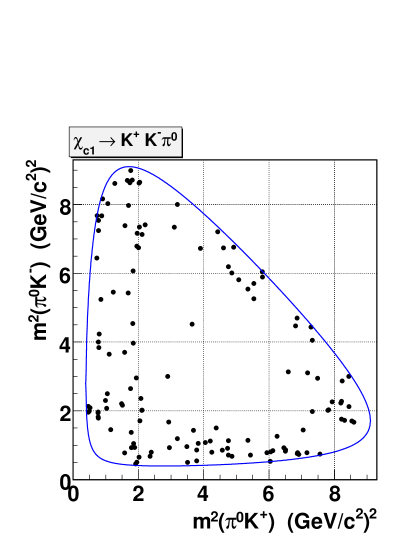
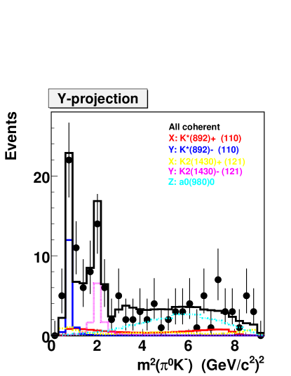
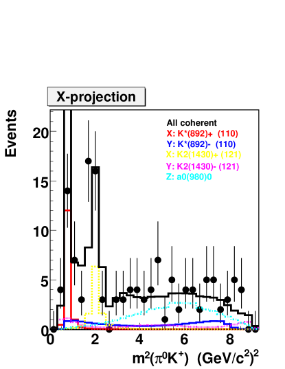
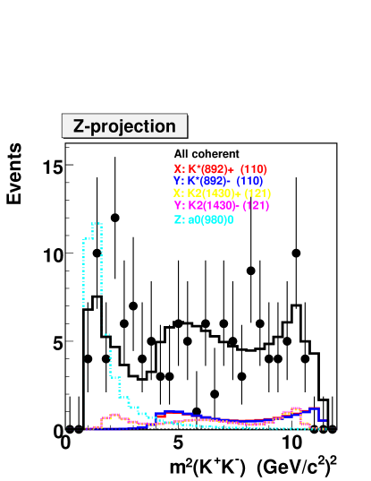
Figure 11: Dalitz plot and projections on the three mass squared combinations for $\chi_{c1}\to K^{+}K^{-}\pi^{0}$. The displayed fit projections are described in the text.

for $\chi_{c1}\to\pi^{+}K^{-}K^{0}_{S}$ in Figure 12.

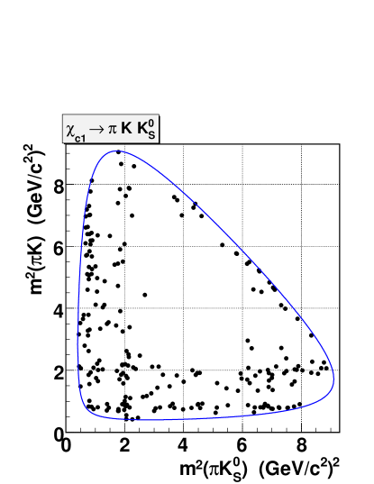
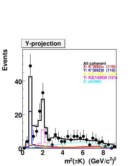
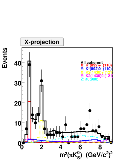
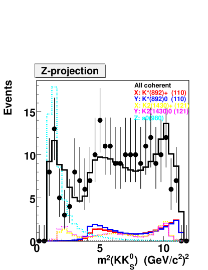
Figure 12: Dalitz plot and projections on the three mass squared combinations for $\chi_{c1}\to\pi^{+}K^{-}K^{0}_{S}$. The displayed fit projections are described in the text.

We do a combined Dalitz plot analysis to these modes taking advantage of isospin symmetry. An isospin Clebsch-Gordan decomposition for these decays, Appendix I, Equations 11, 12, and 20, shows that these two Dalitz plots should have the same set of amplitude and phase parameters for all $K^{*}\overline{K}$ and $a_{0}(980)\pi$ intermediate states. The relative factor $-\sqrt{2}$ between two Dalitz plot amplitudes does not matter due to the individual normalization of their probability density functions. In the combined fit to these two Dalitz plots, we use the following constraints on amplitudes and phases: $a_{K^{*+}}=a_{K^{*-}}=a_{K^{*0}}=a_{\overline{K^{*0}}}\equiv a_{K^{*}}$, $\phi_{K^{*+}}=\phi_{K^{*-}}=\phi_{K^{*0}}=\phi_{\overline{K^{*0}}}\equiv\phi_{K^{*}}$, $a_{a(980)^{+}}=a_{a(980)^{-}}=a_{a(980)^{0}}\equiv a_{a(980)}$, and $\phi_{a(980)^{+}}=\phi_{a(980)^{-}}=\phi_{a(980)^{0}}\equiv\phi_{a(980)}$. The overall amplitude normalization and one phase are arbitrary parameters and we set $a_{K^{*}(892)}=1$ and $\phi_{K^{*}(892)}=0$.

The limited size of this sample, even in the combined Dalitz plot analysis, and the many possible contributing resonances leave us unable to draw clear conclusions. Visual inspection shows apparent contributions from $K^{*}(892)^{\pm}K^{\mp}$, $K^{*}(892)^{0}K^{0}_{S}$, $K^{*}(1430)^{\pm}K^{\mp}$, $K^{*}(1430)^{0}K^{0}_{S}$, $a_{0}(980)^{0}\pi^{0}$, and $a_{0}(980)^{\pm}\pi^{\mp}$. It is not clear if the $K^{*}(1430)$ are $K^{*}_{0}$ or $K^{*}_{2}$, and many other $K\pi$ and $KK$ resonances can possibly contribute. Our best fit preliminary result is shown in Table 6 showing

Table 6: Preliminary results of the combined fits to the $\chi_{c1}\to K^{+}K^{-}\pi^{0}$ and $\chi_{c1}\to K^{0}_{S}K\pi$ Dalitz plots.

Contribution	Amplitude	Phase (∘)	Fit Fraction (%)
$K^{*}(892)K$	1	0	$19.7\pm 4.0\pm 2.0$
$K^{*}_{2}(1430)K$	$0.50\pm 0.09\pm 0.12$	$-2\pm 13\pm 6$	$18.0\pm 6.6\pm 3.2$
$K^{*}_{0}(1430)K$	$5.3\pm 1.0\pm 0.1$	$77\pm 12\pm 16$	$36.0\pm 12.8\pm 3.0$
$K^{*}(1680)K$	$2.3\pm 0.5\pm 0.5$	$-38\pm 12\pm 12$	$11.2\pm 5.4\pm 2.7$
$a_{0}(980)\pi$	$10.8\pm 1.2\pm 1.2$	$-112\pm 12\pm 3$	$29.5\pm 7.1\pm 2.6$

statistical and systematic errors. This fit has a good probability of matching the data, 32.1%, and agrees with fits done to the separate Dalitz plots not taking advantage of isospin symmetry. Unfortunately we can change our decay model by swapping the $K^{*}(1430)$ plus $K^{*}(1680)$ contributions for a flat non-resonant background, or a $\kappa$ and get fits of lower, but still acceptable, probability of matching the data. We also find that an alternative solution using the same set of contributions fits the data acceptably, but less well than the displayed result. This alternative result disagrees with the nominal result by more than the statistical uncertainties should allow. We conclude that our $\chi_{c1}\to KK\pi$ sample is too small to extract the resonant substructure. We do clearly see contributions from $K^{*}(892)K$ and $a_{0}(980)\pi$ at roughly the 20% and 30% level respectively. The balance of the Dalitz plots are probably from higher mass $K\pi$ resonances.

In conclusion we have searched for and studied selected three body hadronic decays of the $\chi_{c0}$, $\chi_{c1}$, $\chi_{c2}$ produced in radiative decays of the $\psi(2S)$ in $e^{+}e^{-}$ collisions observed with the CLEO detector. Our preliminary observations and branching fraction limits are summarized in Table 4. In $\chi_{c1}\to\pi^{+}\pi^{-}\eta$ we have studied the resonant substructure using a Dalitz plot analysis, and our preliminary results are summarized in Table 5. Similarly in $\chi_{c1}\to KK\pi$ we clearly see contributions from $K^{*}(892)K$ and $a_{0}(980)\pi$ at roughly the 20% and 30% level respectively.

We gratefully acknowledge the effort of the CESR staff in providing us with excellent luminosity and running conditions. D. Cronin-Hennessy and A. Ryd thank the A.P. Sloan Foundation. This work was supported by the National Science Foundation, the U.S. Department of Energy, and the Natural Sciences and Engineering Research Council of Canada.

I Appendix: Clebsch-Gordan decomposition for $\chi_{c1}$

In order to constrain amplitudes and phases in $\chi_{c1}$ decays we use a Clebsch-Gordan decomposition of the $\chi_{c1}$ (the state with $|I=0,I_{Z}=0\rangle$) for possible isospin subsystems:

$$\chi_{c1}\to(K\pi)_{I=1/2}{\overline{K}},$$ (2)

$$\chi_{c1}\to({\overline{K}}\pi)_{I=1/2}K,$$ (3)

$$\chi_{c1}\to(K{\overline{K}})_{I=1}\pi.$$ (4)

Below we use Clebsch-Gordan decomposition rules, $|J,M\rangle=\sum_{f}c_{f}|m_{1},m_{2}\rangle_{f}$ from Ref. pdg .

I.1 Clebsch-Gordan decomposition for $K^{*}\to K\pi$ decays

We assume that $K^{*}$s with I=1/2 form two isodoublets: ($K^{*+}$, $K^{*0}$) and ($\overline{K^{*0}}$, $K^{*-}$) with ($I_{Z}=\frac{1}{2}$,$I_{Z}=-\frac{1}{2}$) respectively. The Clebsch-Gordan decomposition rules for isospin states of product particles $\mathbf{1\times\frac{1}{2}}$ are:

$|\frac{1}{2},\frac{1}{2}\rangle=\sqrt{\frac{2}{3}}|1,-\frac{1}{2}\rangle-\sqrt{\frac{1}{3}}|0,\frac{1}{2}\rangle$

$|\frac{1}{2},-\frac{1}{2}\rangle=\sqrt{\frac{1}{3}}|0,-\frac{1}{2}\rangle-\sqrt{\frac{2}{3}}|-1,\frac{1}{2}\rangle$

$$K^{*+}=|\frac{1}{2},\frac{1}{2}\rangle=\sqrt{\frac{2}{3}}\pi^{+}K^{0}-\sqrt{\frac{1}{3}}\pi^{0}K^{+},$$ (5)

$$K^{*0}=|\frac{1}{2},-\frac{1}{2}\rangle=\sqrt{\frac{1}{3}}\pi^{0}K^{0}-\sqrt{\frac{2}{3}}\pi^{-}K^{+},$$ (6)

$$\overline{K^{*0}}=|\frac{1}{2},\frac{1}{2}\rangle=\sqrt{\frac{2}{3}}\pi^{+}K^{-}-\sqrt{\frac{1}{3}}\pi^{0}\overline{K^{0}},$$ (7)

$$K^{*-}=|\frac{1}{2},-\frac{1}{2}\rangle=\sqrt{\frac{1}{3}}\pi^{0}K^{-}-\sqrt{\frac{2}{3}}\pi^{-}\overline{K^{0}}.$$ (8)

I.2 Cases of $\chi_{c1}\to(K\pi)_{I=1/2}{\overline{K}}$ and $\chi_{c1}\to({\overline{K}}\pi)_{I=1/2}K$ decays

For $\chi_{c1}\to K^{*}\overline{K}$ and $\chi_{c1}\to\overline{K^{*}}K$ modes we use $\mathbf{\frac{1}{2}\times\frac{1}{2}}$ rule: $|0,0\rangle=\frac{1}{\sqrt{2}}(|\frac{1}{2},-\frac{1}{2}\rangle-|-\frac{1}{2},\frac{1}{2}\rangle)$

$$\chi_{c1}\to\frac{1}{\sqrt{2}}(K^{*+}K^{-}-K^{*0}\overline{K^{0}}),$$ (9)

$$\chi_{c1}\to\frac{1}{\sqrt{2}}(\overline{K^{*0}}K^{0}-K^{*-}K^{+}).$$ (10)

Combining Equations 9,10 with Equations 5-8 we get

$$\chi_{c1}\sqrt{2}\to\sqrt{\frac{2}{3}}\bigg{[}(\pi^{+}K^{0})K^{-}+(\pi^{-}K^{+})\overline{K^{0}}\bigg{]}-\sqrt{\frac{1}{3}}\bigg{[}(\pi^{0}K^{+})K^{-}+(\pi^{0}K^{0})\overline{K^{0}}\bigg{]},$$ (11)

$$\chi_{c1}\sqrt{2}\to\sqrt{\frac{2}{3}}\bigg{[}(\pi^{+}K^{-})K^{0}+(\pi^{-}\overline{K^{0}})K^{+}\bigg{]}-\sqrt{\frac{1}{3}}\bigg{[}(\pi^{0}K^{-})K^{+}+(\pi^{0}\overline{K^{0}})K^{0}\bigg{]}.$$ (12)

Assuming charge symmetry the amplitudes in Equations 11 and 12 should be equal. From these equations we may get the ratio of rates:

$$\Gamma(\chi_{c1}\to\pi^{+}K^{-}K^{0})/\Gamma(\chi_{c1}\to\pi^{0}K^{+}K^{-})=2,$$ (13)

$$\Gamma(\chi_{c1}\to\pi^{-}K^{+}\overline{K^{0}})/\Gamma(\chi_{c1}\to\pi^{0}K^{+}K^{-})=2,$$ (14)

or their sum

$$\Gamma(\chi_{c1}\to\pi^{+}K^{-}K^{0})+\Gamma(\chi_{c1}\to\pi^{-}K^{+}\overline{K^{0}})=4\Gamma(\chi_{c1}\to\pi^{0}K^{+}K^{-}).$$ (15)

I.3 Case of $\chi_{c1}\to(K{\overline{K}})_{I=1}\pi$ decay

For $\chi_{c1}\to a\pi$ modes we use the $\mathbf{1\times 1}$ rule: $|0,0\rangle=\frac{1}{\sqrt{3}}(|1,-1\rangle-|0,0\rangle+|-1,1\rangle)$

$$\chi_{c1}\to\frac{1}{\sqrt{3}}(a^{+}\pi^{-}-a^{0}\pi^{0}+a^{-}\pi^{+})$$ (16)

For $a\to K{\overline{K}}$ we use the $\mathbf{\frac{1}{2}\times\frac{1}{2}}$ rules:

$a^{+}$: $|1,1\rangle=|\frac{1}{2},\frac{1}{2}\rangle$

$$a^{+}\to K^{+}\overline{K^{0}},$$ (17)

$a^{0}$: $|1,0\rangle=\frac{1}{\sqrt{2}}(|\frac{1}{2},-\frac{1}{2}\rangle+|-\frac{1}{2},\frac{1}{2}\rangle)$

$$a^{0}\to\frac{1}{\sqrt{2}}(K^{+}K^{-}+K^{0}\overline{K^{0}}),$$ (18)

$a^{-}$: $|1,-1\rangle=|-\frac{1}{2},-\frac{1}{2}\rangle$

$$a^{-}\to K^{0}K^{-}.$$ (19)

Combining Equation 16 with Equations 17-19 we get

$$\chi_{c1}\sqrt{3}\to(K^{+}\overline{K^{0}})\pi^{-}-\frac{1}{\sqrt{2}}\bigg{[}(K^{+}K^{-})\pi^{0}+(K^{0}\overline{K^{0}})\pi^{0}\bigg{]}+(K^{0}K^{-})\pi^{+}.$$ (20)

From Equations 20 we may get the ratio of rates:

$$\Gamma(\chi_{c1}\to\pi^{+}K^{-}K^{0})/\Gamma(\chi_{c1}\to\pi^{0}K^{+}K^{-})=2,$$ (21)

$$\Gamma(\chi_{c1}\to\pi^{-}K^{+}\overline{K^{0}})/\Gamma(\chi_{c1}\to\pi^{0}K^{+}K^{-})=2,$$ (22)

or their sum

$$\Gamma(\chi_{c1}\to\pi^{+}K^{-}K^{0})+\Gamma(\chi_{c1}\to\pi^{-}K^{+}\overline{K^{0}})=4\Gamma(\chi_{c1}\to\pi^{0}K^{+}K^{-}).$$ (23)

I.4 Consequences for Dalitz plot analysis

Comparing Equations 13-15 for intermediate states with $K^{*}$ and Equations 21-23 for intermediate states with $a(980)$, one may notice that they are identical. Thus observations of $\pi^{+}K^{-}K^{0}$ and charge conjugated $\pi^{-}K^{+}\overline{K^{0}}$ final states on the same Dalitz plot will yield the same ratio between all $K^{*}$ and $a(980)$ amplitudes for both $K^{0}K^{-}\pi^{+}$ and $K^{+}K^{-}\pi^{0}$ Dalitz plots. The ratio of amplitudes between these two Dalitz plots is $-\sqrt{2}$. The relative negative sign between amplitudes does not matter, because the rates depend on the matrix element squared. The relative factor $\sqrt{2}$ between amplitudes does not matter, because the normalizations are different for each Dalitz plot. This isospin analysis implies that these two Dalitz plots, $K^{0}K^{-}\pi^{+}$ and $K^{+}K^{-}\pi^{0}$, can be parametrized using a common set of parameters for each of $K^{*}$s and $a(980)$ intermediate state with

$$a_{K^{*+}}=a_{K^{*-}}=a_{K^{*0}}=a_{\overline{K^{*0}}}\equiv a_{K^{*}},$$ (24)

$$\phi_{K^{*+}}=\phi_{K^{*-}}=\phi_{K^{*0}}=\phi_{\overline{K^{*0}}}\equiv\phi_{K^{*}},$$ (25)

$$a_{a(980)^{+}}=a_{a(980)^{-}}=a_{a(980)^{0}}\equiv a_{a(980)},$$ (26)

$$\phi_{a(980)^{+}}=\phi_{a(980)^{-}}=\phi_{a(980)^{0}}\equiv\phi_{a(980)}.$$ (27)

II Appendix: The effect of $\chi_{c1}$ polarization

II.1 Angular distributions

In this analysis we use the angular distributions explicitly shown in Table 7 derived for a non-polarized decaying particle ($\chi_{c1}$) in Ref. Filippini-Fontana-Rotondi .

Table 7: Angular distributions.

$J\to j+L$	Probability
0$\to$0+0	uniform
1$\to$0+1	uniform
2$\to$0+2	uniform
0$\to$1+1	$(1+z^{2})\cos^{2}\theta$
0$\to$2+2	$(z^{2}+3/2)^{2}(\cos^{2}\theta-1/3)^{2}$
1$\to$1+0	$1+z^{2}\cos^{2}\theta$
1$\to$1+1	$\sin^{2}\theta$
1$\to$1+2	$1+(3+4z^{2})\cos^{2}\theta$
1$\to$2+1	$(1+z^{2})\big{[}1+3\cos^{2}\theta+9z^{2}(\cos^{2}\theta-1/3)^{2}\big{]}$
1$\to$2+2	$(1+z^{2})\cos^{2}\theta\sin^{2}\theta$ (*)
2$\to$1+1	$3+(1+4z^{2})\cos^{2}\theta$
2$\to$1+2	$\sin^{2}\theta$
2$\to$2+0	$1+z^{2}/3+z^{2}\cos^{2}\theta+z^{4}(\cos^{2}\theta-1/3)^{2}$
2$\to$2+1	$1+z^{2}/9+(z^{2}/3-1)\cos^{2}\theta-z^{2}(\cos^{2}\theta-1/3)^{2}$
2$\to$2+2	$1+z^{2}/9+(z^{2}/3-1)\cos^{2}\theta+(16z^{4}+21z^{2}+9)(\cos^{2}\theta-1/3)^{2}/3$ (*)

(*) These formulas have been derived based on the covariant helicity formalism approach also discussed in Ref. Filippini-Fontana-Rotondi .

The parameters in Table 7 follow the conventions of the original publication: $J$ - spin of the initial particle $J\to j+c$; $j$ - spin of the resonance $j\to a+b$, where $a,b,c$ - spin 0 particles; $L$ - orbital angular momentum between ($j^{p}$) resonance and the recoil particle $c$. A relativistic correction factor $z$ and $\cos\theta$, where $\theta$ is an angle between directions of particles $a$ and $c$ in resonance $j^{p}$ rest frame is discussed in Appendix II.2.

In order to account for the polarization of the initial $\chi_{c1}$ produced in the radiative decay $\psi(2S)\to\gamma\chi_{c1}$, a full Partial Wave Analysis formalism, for example from Ref. BES_PWA_formalism , would be needed. The matrix element amplitudes would depend on additional angular variables in addition to the two invariant squared masses as in the regular Dalitz plot analysis. The number of parameters would also be increased to account for different helicity amplitudes contributions. On the other hand, an expected $\chi_{c1}$ production angular distribution, $\propto 1-\frac{1}{3}\cos^{2}\theta_{\chi_{c1}}$, is $\sim$15% different from uniform and we expect that the effect of polarization is small in the decays under study.

II.2 Expressions for relativistically non-invariant variables in terms of Dalitz plot invariant variables

Although a covariant spin tensor formalism is applied, for simplicity the formulas in Ref. Filippini-Fontana-Rotondi and Table 7 are expressed in terms of relativistically non-invariant variables $z$ and $\cos\theta$. Here we discuss the meaning of these variables and their expression in terms of particle masses and invariant masses.

Assuming the decay $d\to Rc$, $R\to ab$ we may derive kinematic variables used in formulas for angular distribution in terms of Dalitz plot invariant variables. The energy and momentum of particle $a$ in the resonance $R$ or $(ab)$ rest frame is a trivial expression

$$E_{a}=\frac{m_{ab}^{2}+m_{a}^{2}-m_{b}^{2}}{2m_{ab}},~{}~{}~{}~{}P_{a}=\sqrt{E_{a}^{2}-m_{a}^{2}}.$$ (28)

The energy and momentum of particle $c$ in the resonance $R$ rest frame can be obtained from the invariant mass $m_{d}^{2}$ expression in the $R$ rest frame. Indeed, $m_{d}^{2}=(p_{c}+p_{R})^{2}$, in the resonance $R$ rest frame $p_{c}=(E_{c},\vec{P_{c}})$, $p_{R}=(m_{R},\vec{0})$, $\to m_{d}^{2}=m_{c}^{2}+m_{R}^{2}+2m_{R}E_{c}$, hence

$$E_{c}=\frac{m_{d}^{2}-m_{ab}^{2}-m_{c}^{2}}{2m_{ab}},~{}~{}~{}~{}P_{c}=\sqrt{E_{c}^{2}-m_{c}^{2}}.$$ (29)

Now, the $\cos\theta$ between directions of particles $a$ and $c$ in resonance $R$ rest frame can be expressed through the known energies and momenta of particles $a$ and $c$ and their measured invariant mass squared $m_{ac}^{2}$:

$$\cos\theta=\frac{m_{a}^{2}+m_{c}^{2}+2E_{a}E_{c}-m_{ac}^{2}}{2P_{a}P_{c}}.$$ (30)

The resonance energy and relativistic correction factor (used in in Table 7) in the decaying particle $d$ rest frame are:

$$E_{r}=\frac{m_{d}^{2}+m_{ab}^{2}-m_{c}^{2}}{2m_{d}},~{}~{}~{}~{}z^{2}=\gamma^{2}_{R}-1=\frac{E_{r}^{2}}{m_{ab}^{2}}-1.$$ (31)

References

(1) N. Brambilla et al., CERN-2005-005 [hep-ph/0412158] is
a comprehensive recent review of heavy quarkonium physics.
(2) G. Viehhauser et al., CLEO III Operation,
Nucl. Instrum. Methods A 462, 146 (2001).
(3) R.A. Briere et al., (CESR-c and CLEO-c Taskforces, CLEO-c Collaboration),
Cornell University, LEPP Report No. CLNS 01/1742 (2001) (unpublished).
(4) We use a GEANT-3 based full detector response Monte Carlo simulation.
(5) S. Eidelman et al., Physics Letters B592, 1 (2004).
(6) S.B. Athar et al., (CLEO Collaboration), Phys. Rev. D 70, 112002 (2004).
(7) S. Kopp et al., Phys. Rev. D 63, 092001 (2001).
(9) Jose A. Oller, Phys. Rev. D 71, 054030 (2005).
(10) V. Filippini, A. Fontana, and A. Rotondi, PR D51 (1995) 2247.
(11) B.S. Zou and D.V. Bugg, Eur. Phys. J. A16, 537 (2003).