Measurement of the $B^{0}\rightarrow\pi^{-}\ell^{+}\nu$ Form Factor Shape and Branching Fraction, and Determination of $|V_{ub}|$ with a Loose Neutrino Reconstruction Technique

The BABAR Collaboration

We report the results of a study of the exclusive charmless semileptonic $B^{0}\rightarrow\pi^{-}\ell^{+}\nu$ decay undertaken with approximately 227 million $B\bar{B}$ pairs collected at the $\mathchar 28935\relax{(4S)}$ resonance with the BABAR detector. The analysis uses events in which the signal $B$ mesons are reconstructed with a novel loose neutrino reconstruction technique. We obtain partial branching fractions in 12 bins of $q^{2}$, the $\ell^{+}\nu$ invariant mass squared, from which we extract the $f^{+}(q^{2})$ form factor shape and the total branching fraction: ${{\cal B}}(B^{0}\rightarrow\pi^{-}\ell^{+}\nu)$ $=(1.44\pm 0.08_{stat}\pm 0.10_{syst})\times 10^{-4}$. Based on a recent theoretical calculation of the form factor, we find the magnitude of the CKM matrix element $|V_{ub}|$ to be $\left(4.1\pm 0.2_{stat}\pm 0.2_{syst}{}^{+0.6}_{-0.4}{}_{\mathrm{FF}}\right)\times{10^{-3}}$, where the last uncertainty is due to the normalization of the form factor.

1 Introduction

The precise measurement of $|V_{ub}|$, the smallest element of the CKM matrix [1], will strongly constrain the description of weak interactions and CP violation in the Standard Model.

The measurement of $|V_{ub}|$ requires the study of a $b\rightarrow u$ transition in a well-understood context. Semileptonic $b\rightarrow u\ell\nu$ decays (here, $\ell$ stands for an electron or a muon) are best for that purpose since they are much easier to understand theoretically than hadronic decays, and they are much easier to study experimentally than the less abundant purely leptonic decays.

For $B^{0}\rightarrow\pi^{-}\ell^{+}\nu$ decays, the theoretical description of the quarks’ strong interactions is parametrized by a single form factor, $f^{+}(q^{2})$, where $q^{2}$ is the squared invariant mass of the $\ell^{+}\nu$ system. Only the shape of $f^{+}(q^{2})$ can be measured experimentally. Its normalization is provided by theoretical calculations which currently suffer from relatively large uncertainties and, often, do not agree with each other. As a result, the normalization of the $f^{+}(q^{2})$ form factor is the largest source of uncertainty in the extraction of $|V_{ub}|$ from the $B^{0}\rightarrow\pi^{-}\ell^{+}\nu$ branching fraction. Values of $f^{+}(q^{2})$ for $B^{0}\rightarrow\pi^{-}\ell^{+}\nu$ decays are provided by unquenched [3, 4] and quenched [5] lattice QCD (LQCD) calculations, presently reliable only at high $q^{2}$ ($>16$ ${\mathrm{\,Ge\kern-1.00006ptV^{2}\!/}c^{4}}$), and by Light Cone Sum Rules calculations [6] (LCSR), based on approximations only valid at low $q^{2}$ ($<16$ ${\mathrm{\,Ge\kern-1.00006ptV^{2}\!/}c^{4}}$), as well as by a quark model [7]. The QCD theoretical predictions are at present more precise for $B^{0}\rightarrow\pi^{-}\ell^{+}\nu$ decays than for other exclusive $B\rightarrow X_{u}\ell\nu$ decays. Experimental data can be used to discriminate between the various calculations by measuring the $f^{+}(q^{2})$ shape precisely, thereby leading to a smaller theoretical uncertainty on $|V_{ub}|$.

The present analysis of $B^{0}\rightarrow\pi^{-}\ell^{+}\nu$ decays aims to obtain an accurate measurement of the $f^{+}(q^{2})$ shape in order to extract a more precise value of $|V_{ub}|$ from the measurement of the total $B^{0}\rightarrow\pi^{-}\ell^{+}\nu$ branching fraction, ${{\cal B}}(B^{0}\rightarrow\pi^{-}\ell^{+}\nu)$. To do so, we extract the $B^{0}\rightarrow\pi^{-}\ell^{+}\nu$ yields in 12 bins of $\tilde{q}^{2}$ using a loose neutrino reconstruction technique and $\tilde{q}^{2}$-dependent cuts. The quantity $\tilde{q}^{2}$ denotes the uncorrected measured value of $q^{2}$ and will be referred to as “raw”. The final $q^{2}$ spectrum is corrected for reconstruction effects by applying an unfolding algorithm to the measured $\tilde{q}^{2}$ spectrum. The total ${{\cal B}}(B^{0}\rightarrow\pi^{-}\ell^{+}\nu)$ is given by the sum of the partial branching fractions $\Delta{{\cal B}}(B^{0}\rightarrow\pi^{-}\ell^{+}\nu,q^{2})$. The $q^{2}$ shape of the $f^{+}(q^{2})$ form factor is obtained from the normalized partial branching fractions $\mbox{$\Delta\cal B$}(q^{2})/{\cal B}$ spectrum combined with two covariance matrices (one for the statistical errors and one for the systematic errors) which give the correlations among the values of $\mbox{$\Delta\cal B$}(q^{2})/{\cal B}$ measured in the different $q^{2}$ bins. The measured $\mbox{$\Delta\cal B$}(q^{2})/{\cal B}$ spectrum is fitted to a model-dependent parametrization [8] of the $f^{+}(q^{2})$ form factor. The model-independent $\mbox{$\Delta\cal B$}(q^{2})/{\cal B}$ spectrum and its correlation matrices are given explicitly to allow future studies with different $f^{+}(q^{2})$ parametrizations using the present data. The value of the CKM matrix element $|V_{ub}|$ is then derived from the form factor calculations, combined with the measured $\Delta\cal B$$s$.

The main innovation of this analysis is the use of a loose neutrino reconstruction technique which yields a much higher signal reconstruction efficiency than in past measurements, while keeping the systematic errors at a relatively low level. The higher yield allows the utilization of a large number of $q^{2}$ bins and the determination of the background composition using several independent fit parameters. In addition, we use $\tilde{q}^{2}$-dependent cuts and estimate the $f^{+}(q^{2})$ shape systematic error.

The data used in this analysis were collected with the BABAR detector at the PEP-II asymmetric $e^{+}e^{-}$ collider. The BABAR detector is described elsewhere [9]. The following samples are used: 206.4 $\mbox{\,fb}^{-1}$  integrated luminosity of data collected at the $\mathchar 28935\relax{(4S)}$ resonance, corresponding to 227.4 million $B\bar{B}$ decays; 27.0 $\mbox{\,fb}^{-1}$ integrated luminosity of data collected approximately 40 $\mathrm{\,Me\kern-1.00006ptV}$ below the $\mathchar 28935\relax{(4S)}$ resonance (denoted “off-resonance data” hereafter); standard BABAR Monte Carlo (MC) simulation using GEANT4 [10] and EvtGen [11]; 1.64 million $B^{0}\rightarrow\pi^{-}\ell^{+}\nu$ signal events using the FLATQ2 generator [12]; 2.02 billion generic $B^{0}\bar{B^{0}}$ and $B^{+}B^{-}$ events, and 2.44 billion generic $u\bar{u}/d\bar{d}/s\bar{s}/c\bar{c}$ and $\tau^{+}\tau^{-}$ “continuum” events.

2 Analysis Method

Values of $|V_{ub}|$ have previously been extracted from $B^{0}\rightarrow\pi^{-}\ell^{+}\nu$ measurements by CLEO [13, 14], BABAR [15, 16] and BELLE [17]. Our analysis is based on a novel technique denoted “loose neutrino reconstruction”. The main motivation for implementing this technique is to maximize the extracted $B^{0}\rightarrow\pi^{-}\ell^{+}\nu$ signal yields in order to measure the $f^{+}(q^{2})$ shape as precisely as possible.

Even though $B$ mesons are always produced in pairs at the $\mathchar 28935\relax{(4S)}$ resonance, a major feature of the neutrino reconstruction technique is that the decay of the non-signal $B$ is not reconstructed. Instead, the signal $B$ mesons are directly identified using the measured $\pi^{\pm}$ and $\ell^{\mp}$ tracks together with the events’ missing momentum as an approximation to the signal neutrino momentum [13, 14, 15]. The neutrino four-momentum, $P_{miss}=(|\vec{p}_{miss}|,\vec{p}_{miss})$, is inferred from the difference between the four-momentum of the colliding-beam particles, $P_{\rm beams}=(E_{\rm beams},\vec{p}_{\rm beams})$, and the sum of the four-momenta of all charged and neutral particles detected in a single interaction, $P_{tot}=(E_{tot},\vec{p}_{tot})$, such that $\vec{p}_{miss}=\vec{p}_{\rm beams}-\vec{p}_{tot}$. Compared with the tagged analyses described in Refs. [16, 17], the neutrino reconstruction approach yields a lower signal purity but a significant increase in the signal reconstruction efficiency. The new approach used in the loose neutrino reconstruction further increases this efficiency compared with the previous untagged analyses [13, 14, 15] by avoiding neutrino quality cuts (for example, a tight cut on the invariant missing mass to ensure the neutrino properties are well taken into account). Such cuts were required to allow the calculation of $\tilde{q}^{2}=(P_{\ell}+P_{\nu})^{2}$. To obtain the values of $\tilde{q}^{2}$, we use instead the neutrino-independent relation: $\tilde{q}^{2}=(P_{B}-P_{\pi})^{2}$. Although this relation is strictly true and Lorentz invariant, it cannot be used directly because the value of $P_{B}$ is not known. Only the value of $P_{\pi}$, measured in the laboratory frame, and that of the $\mathchar 28935\relax{(4S)}$ 4-momentum are known. Nevertheless, since the $B$ momentum is small in the $\mathchar 28935\relax{(4S)}$ frame, a common approximation is to boost the pion to the $\mathchar 28935\relax{(4S)}$  frame and use the relation $\tilde{q}^{2}=(P_{B}-P_{\pi})^{2}$ in that frame, where the $B$ meson is assumed to be at rest.

However, a more accurate value of $\tilde{q}^{2}$ can be obtained in the so-called $Y$-average frame [18, 19] where the pseudo-particle $Y$ has a 4-momentum defined by $P_{Y}\equiv(P_{\pi}+P_{\ell})$. The angle $\theta_{BY}$ between the directions of the $p^{*}_{B}$ and $p^{*}_{Y}$ momenta in the $\mathchar 28935\relax{(4S)}$ rest frame can be determined assuming energy-momentum conservation in a semileptonic $B\rightarrow Y\nu$ decay. Its value is given by: $\cos\theta_{BY}=\left(2E^{*}_{B}E^{*}_{Y}-m_{B}^{2}-m_{Y}^{2}\right)/\left(2|\vec{p}^{\,*}_{B}||\vec{p}^{\,*}_{Y}|\right)$, where $m_{B},m_{Y},E^{*}_{B}$, $E^{*}_{Y},\vec{p}^{\,*}_{B}$ and $\vec{p}^{\,*}_{Y}$ refer to the masses, energies and momenta of the $B$ meson and the $Y$ “particle”. Thus, in the $\mathchar 28935\relax{(4S)}$ frame, a cone is defined whose axis is given by the direction of the $Y$ momentum with the half-angle subtended at the apex given by $\theta_{BY}$. The apex corresponds to the vertex formed by the $Y$ and $B$ momenta directions. The $B$ momentum lies somewhere on the surface of the cone and thus its position is known only up to an azimuthal angle $\phi$ defined with respect to the $Y$ momentum. The value of $\tilde{q}^{2}$ in the $Y$-average frame is computed as follows: it first assumes that the $B$ rest frame is located at an arbitrary angle $\phi_{0}$, and the value of $q_{0}^{2}$ is calculated in that specific frame position. The values of $q^{2}_{1}$, $q^{2}_{2}$ and $q^{2}_{3}$ are then calculated with the $B$ rest frame at $\phi_{1}=\phi_{0}+90^{o}$, $\phi_{2}=\phi_{0}+180^{o}$ and $\phi_{3}=\phi_{0}+270^{o}$, respectively. The value of $\tilde{q}^{2}$ in the $Y$-average frame is then defined as $\tilde{q}^{2}=\frac{q^{2}_{0}+q^{2}_{1}+q^{2}_{2}+q^{2}_{3}}{4}$. Using more than four values of $\phi_{i}$ does not significantly improve the $\tilde{q}^{2}$ resolution.

The use of the $Y$-average frame yields a $q^{2}$ resolution that is approximately 20% better than what is obtained in the usual $\mathchar 28935\relax{(4S)}$ frame where the $B$ meson is assumed to be at rest. We get an unbiased $q^{2}$ resolution of 0.52 ${\mathrm{\,Ge\kern-1.00006ptV^{2}\!/}c^{4}}$ when the selected pion candidate comes from a $B^{0}\rightarrow\pi^{-}\ell^{+}\nu$ decay (Fig. 1), which accounts for approximately 91% of our signal candidates after all the analysis selections. When a track from the non-signal $B$ is wrongly selected as the signal pion, the $q^{2}$ resolution becomes very poor and biased.

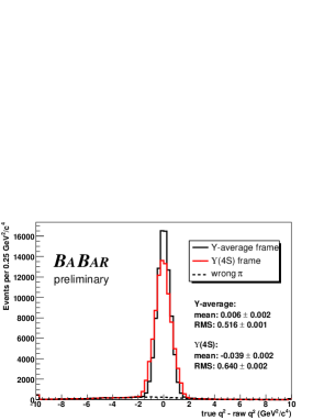
Figure 1: $q^{2}$ resolution of $B^{0}\rightarrow\pi^{-}\ell^{+}\nu$ signal events obtained in the Y-average and $\mathchar 28935\relax{(4S)}$  frames after all analysis cuts and MC corrections. The very long tail arises when a track coming from the non-signal $B$ is wrongly selected as the signal pion. The numbers of entries in the first and last bins correspond to the sum of all entries with $\Delta q^{2}<-9.75$ ${\mathrm{\,Ge\kern-1.00006ptV^{2}\!/}c^{4}}$ and $\Delta q^{2}>9.75$ ${\mathrm{\,Ge\kern-1.00006ptV^{2}\!/}c^{4}}$, respectively.

We correct for our imperfect $q^{2}$ resolution with a $q^{2}$-unfolding algorithm. This algorithm was validated with statistically independent signal MC samples. After all selections, the total signal MC sample contains approximately 120000 events. Five thousand such signal events were used to produce the raw $\tilde{q}^{2}$ and true $q^{2}$ histograms. The remaining signal events were used to build the two unfolding matrices, using the simulated signal events reweighted [12] either to reproduce the $f^{+}(q^{2})$ shape measured in Ref. [15] or with the weights calculated in Ref. [7]. As illustrated in Fig. 2, the true and raw yield distributions differ considerably for various values of $q^{2}$. However, the unfolded values of $q^{2}$ match the true values within the statistical uncertainties of the unfolding procedure, independently of the signal generator used to compute the detector response matrix. This shows that the $q^{2}$-unfolding procedure works as expected.

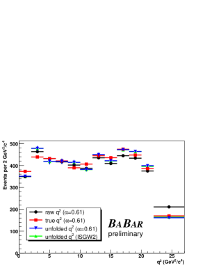
Figure 2: Validation of the $q^{2}$-unfolding procedure. The true and raw yield distributions differ considerably for various values of $q^{2}$. However, independently of the signal generator used to compute the detector response matrix, the unfolded values of $q^{2}$ match the true values within the statistical uncertainties of the unfolding procedure.

To separate the $B^{0}\rightarrow\pi^{-}\ell^{+}\nu$ signal from the backgrounds, we require two well reconstructed tracks that fulfill tight lepton and pion identification criteria. The electron (muon) tracks are required to have a momentum greater than 0.5 (1.0) ${\mathrm{\,Ge\kern-1.00006ptV\!/}c}$ in the laboratory frame. We do not cut on the pion momentum because it is very strongly correlated with $q^{2}$. The kinematic compatibility of the lepton and pion with a real $B^{0}\rightarrow\pi^{-}\ell^{+}\nu$ decay is constrained by requiring that a geometrical vertex fit [20] of the two tracks gives a $\chi^{2}$ probability greater than 0.01, and by requiring that $-1<\cos\theta_{BY}<1$. Note that cuts whose values depend on the measured value of $\tilde{q}^{2}$ (Fig. 3) give the best background rejection. Non-$B\kern 1.79993pt\overline{\kern-1.79993ptB}{}$ events are suppressed by several conditions: we require at least four charged tracks in each event; we require the ratio of the second to the zeroth Fox-Wolfram moments [21] to be less than 0.5; we require the cosine of the angle between the $Y$’s thrust axis and the rest of the event’s thrust axis, $\cos\theta_{thrust}$, to satisfy the relation $\cos\theta_{thrust}<0.460+0.0576\cdot\tilde{q}^{2}-0.00215\cdot\tilde{q}^{4}$ (Fig. 3); we require the polar angle associated with $\vec{p}_{miss}$ to satisfy the relation 2.7 rad $>\theta_{miss}>(0.512-0.0162\cdot\tilde{q}^{2}+0.000687\cdot\tilde{q}^{4})$ rad (Fig. 3). Radiative Bhabha events are rejected using the criteria given in Ref. [22] and photon conversion events are vetoed. Finally, although the shapes of the $\tilde{q}^{2}$, $\Delta E$ and $m_{\rm ES}$ distributions in off-resonance data are very well reproduced by MC simulation in all lepton channels, there is an excess of nearly a factor of two in the yield values observed in data compared to the simulation in the electron/positron channels. We then require $\frac{\vec{p}_{tot}\cdot\hat{z}}{E_{tot}}<0.64$ and $\frac{\vec{p}_{tot}\cdot\hat{z}}{E_{tot}}>0.35$ for candidates in the electron and positron channels, respectively, where the $z$ axis is given by the electron beam direction [9]. This reduces the observed excess by removing additional radiative Bhabha events as well as “two-photon” processes which are not included in the simulated continuum.

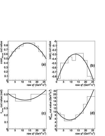
Figure 3: Cut functions used in the analysis, for the variables $\cos\theta_{thrust}$ (a), $\cos\theta_{\ell}$ (b), $\theta_{miss}$ (c) and $M^{2}_{miss}$ (d). The solid curves show the cut values as a function of $\tilde{q}^{2}$. The histograms show the statistically optimal cut values obtained in 10 $\tilde{q}^{2}$ bins based on the minimization of the quantity $\sqrt{(S+B)}/S$ in the $\Delta E$-$m_{\rm ES}$ signal region, where $S$ represents the simulated signal yield and $B$ stands for the simulated background yield.

To reject background $B\bar{B}$ events, we require the Y candidates to have $\cos\theta_{\ell}<0.85$ and $\cos\theta_{\ell}>-0.938+0.0994\cdot\tilde{q}^{2}-0.00384\cdot\tilde{q}^{4}$ (Fig. 3), where $\theta_{\ell}$ is the helicity angle of the W boson [23] reconstructed in the Y-average frame approximation. We reject ${J\mskip-3.0mu/\mskip-2.0mu\psi\mskip 2.0mu}\rightarrow\mu^{+}\mu^{-}$ decays, which can often be mistaken for $B^{0}\rightarrow\pi^{-}\mu^{+}\nu$ decays, by removing candidates with $3.07<m_{Y}<3.13$ ${\mathrm{\,Ge\kern-1.00006ptV\!/}c^{2}}$. Of all the neutrino quality cuts utilized in Refs. [13, 14, 15], only the loose $\tilde{q}^{2}$-dependent criterion on the squared invariant mass of $P_{miss}$ is used: $M^{2}_{miss}<(10.2-1.12\cdot\tilde{q}^{2}+0.0625\cdot\tilde{q}^{4})$ ${\mathrm{\,Ge\kern-1.00006ptV^{2}\!/}c^{4}}$  (Fig. 3). We discriminate against the remaining backgrounds using the variables $\Delta E=(p_{B}\cdot p_{\rm beams}-s/2)/\sqrt{s}$ and $m_{\rm ES}=\sqrt{(s/2+\vec{p}_{B}\cdot\vec{p}_{\rm beams})^{2}/E_{\rm beams}^{2}-\vec{p}_{B}^{\,2}}+(5.29{\mathrm{\,Ge\kern-1.00006ptV\!/}c^{2}}\ -\sqrt{s}/2)$, where $\sqrt{s}$ is the total energy in the $\mathchar 28935\relax{(4S)}$ center-of-mass frame. Only candidates with $|\Delta E|<1.0~{}\mathrm{\,Ge\kern-1.00006ptV}\mbox{ and }m_{\rm ES}>5.19~{}{\mathrm{\,Ge\kern-1.00006ptV\!/}c^{2}}$ are retained. When several candidates remain in an event after the above cuts, we select the candidate with $\cos\theta_{\ell}$ closest to zero and reject the others. This rejects 30% of the combinatorial signal candidates while conserving 97% of the correct ones and reduces the sensitivity of our analysis to the simulation of the candidates’ multiplicity. After all cuts, the total signal event reconstruction efficiency varies between 6.6% and 9.7%, depending on the $q^{2}$ bin, as shown in Fig. 4.

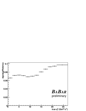
Figure 4: Signal efficiency as a function of true $q^{2}$.

To obtain the $B^{0}\rightarrow\pi^{-}\ell^{+}\nu$ signal yield in each of the 12 reconstructed $\tilde{q}^{2}$ bins, we perform a 2+1 dimensional ($\Delta E$-$m_{\rm ES}$, $q^{2}$) extended binned maximum likelihood fit based on a method developed by Barlow and Beeston [24]. The fitted data samples in each $\tilde{q}^{2}$ bin are divided into four categories: $B^{0}\rightarrow\pi^{-}\ell^{+}\nu$ signal and three backgrounds, $b\rightarrow u\ell\nu$, other $B\bar{B}$, and continuum. The distinct structure of these four types of events in the 2-dimensional $\Delta E$-$m_{\rm ES}$ plane is illustrated in Fig. 5. Since the correlation between $\Delta E$ and $m_{\rm ES}$ cannot be neglected and is difficult to parametrize, we use the $\Delta E$-$m_{\rm ES}$ histograms obtained from the MC simulation as two-dimensional probability density functions (PDF). The simulated signal events are reweighted [12] to reproduce the $f^{+}(q^{2})$ shape measured in Ref. [15]. The $\tilde{q}^{2}$ shape of the simulated non-$B\kern 1.79993pt\overline{\kern-1.79993ptB}{}$ continuum background is scaled to match the off-resonance data control sample containing both $e^{\pm}$ and $\mu^{\pm}$ events, while the scaling of the yields requires separate $e^{\pm}$ and $\mu^{\pm}$ samples. The fit of the MC PDFs to the experimental data gives the values of twenty parameters: twelve parameters for the twelve signal $\tilde{q}^{2}$ bins, three for the $b\rightarrow u\ell\nu$ background, four for the other $B\bar{B}$ background, and one for the continuum background, as illustrated in Fig. 6. The number and type of fit parameters were chosen to provide a good balance between reliance on simulation predictions, complexity of the fit and total error size. The corresponding $\Delta E$ and $m_{\rm ES}$ fit projections in each $\tilde{q}^{2}$ bin for the experimental data are shown in Figs. 7 and 8. We obtain a total signal yield of $5047\pm 251$ events, while for backgrounds the $b\rightarrow u\ell\nu$ yield is $10015\pm 548$ events, the other $B\bar{B}$ yield is $32788\pm 445$ events, and the continuum yield is $9801\pm 467$ events. The fit has a $\chi^{2}$ value of 428/388 degrees of freedom. In the more restricted signal region ($\mbox{$m_{\rm ES}$}>5.272$ ${\mathrm{\,Ge\kern-1.00006ptV\!/}c^{2}}$, $|\mbox{$\Delta E$}|<0.18$ $\mathrm{\,Ge\kern-1.00006ptV}$), the total signal yield is $1340\pm 40$ events and the total background yield $2527\pm 55$ events, for a signal/background ratio of $0.53\pm 0.02$.

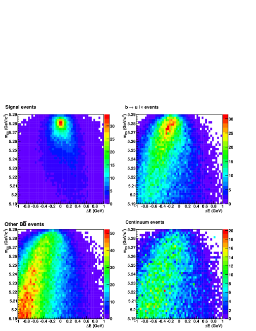
Figure 5: Sum of $\Delta E$-$m_{\rm ES}$ distributions over all 12 bins of $\tilde{q}^{2}$ for the four types of events used in the signal extraction fit after all cuts.

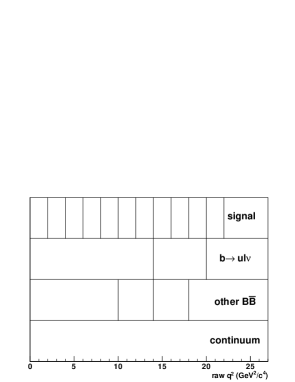
Figure 6: $\tilde{q}^{2}$ binning used in the fit of the MC PDFs to the experimental data.

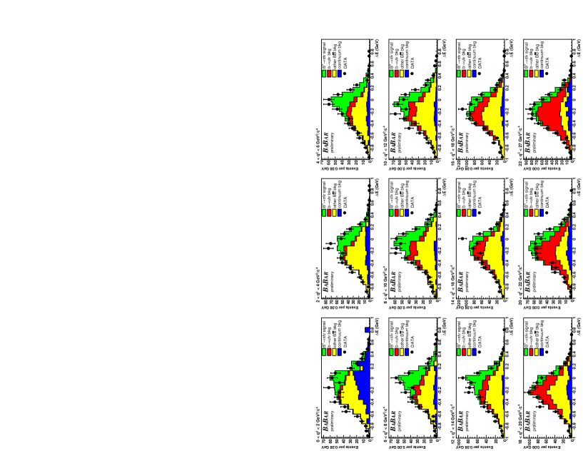
Figure 7: $\Delta E$ yield fit projections obtained in 12 $\tilde{q}^{2}$ bins from the fit to the experimental data, using the full $\Delta E$-$m_{\rm ES}$ fit region. However, the displayed distributions are those after the cut: $m_{ES}>5.272$ ${\mathrm{\,Ge\kern-1.00006ptV\!/}c^{2}}$.

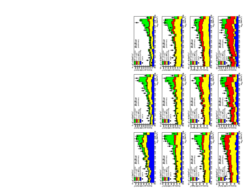
Figure 8: $m_{\rm ES}$ yield fit projections obtained in 12 $\tilde{q}^{2}$ bins from the fit to the experimental data, using the full $\Delta E$-$m_{\rm ES}$ fit region. However, the displayed distributions are those after the cut: $|\Delta E|<0.18$ $\mathrm{\,Ge\kern-1.00006ptV}$.

From the raw signal yields, the unfolded partial branching fractions $\Delta{{\cal B}}(B^{0}\rightarrow\pi^{-}\ell^{+}\nu,q^{2})$ are calculated using the inverted detector response matrix given by the simulation and the signal efficiencies. The total branching fraction ${{\cal B}}(B^{0}\rightarrow\pi^{-}\ell^{+}\nu)$ is given by the sum of the partial $\Delta{{\cal B}}(B^{0}\rightarrow\pi^{-}\ell^{+}\nu,q^{2})$ thereby greatly reducing the sensitivity of the total branching fraction to the uncertainties of the $f^{+}(q^{2})$ form factor values, which have a small but non-negligeable effect on the values of the efficiencies.

To reduce the uncertainties in evaluating the $f^{+}(q^{2})$ shape, instead of fitting the measured $\Delta{{\cal B}}(B^{0}\rightarrow\pi^{-}\ell^{+}\nu,q^{2})$ spectrum, we fit the normalized distribution, $\mbox{$\Delta\cal B$}(q^{2})/{\cal B}$, obtained by dividing the measured $\Delta\cal B$ spectrum by the measured value of the total branching fraction. With this approach, a number of correction factors cancel out, leading to a significant decrease in the systematic error. We fit the $\mbox{$\Delta\cal B$}(q^{2})/{\cal B}$ spectrum using a PDF based on the $f^{+}(q^{2},\alpha)$ parametrization of Becirevic-Kaidalov [8], which is proportional to the standard differential decay rate for a semileptonic $B$ decay to a pseudo-scalar meson ($X_{PS}$):

$$F(q^{2},\alpha)=\frac{|\vec{p_{\pi}}|^{3}\cdot|f^{+}(q^{2},\alpha)|^{2}}{\int_{0}^{q_{max}}|\vec{p_{\pi}}|^{3}\cdot|f^{+}(q^{2},\alpha)|^{2}~{}dq^{2}}~{}~{}\propto\frac{d\Gamma(B\rightarrow X_{PS}~{}\ell^{+}\nu_{\ell})}{dq^{2}}$$ (1)

where $|\vec{p_{\pi}}|=\sqrt{\frac{(m_{B}^{2}+m_{\pi}^{2}-q^{2})^{2}}{4m_{B}^{2}}-m_{\pi}^{2}}$, and the $f^{+}(q^{2},\alpha)$ function is:

$$f^{+}(q^{2},\alpha)=\frac{f_{0}}{(1-q^{2}/m^{2}_{B^{*}})\cdot(1-\alpha q^{2}/m^{2}_{B^{*}})}$$ (2)

The value of $f_{0}$ cancels out in Eq. 1. Note that the data can also be used to extract the $f^{+}(q^{2})$ shape parameter(s) using any theoretical parametrization, e.g. those of Refs. [3, 25, 26]. The $\chi^{2}$ value minimized in the fit is defined in terms of the covariance matrix $U$ to take into account the correlations between the measurements in the various $q^{2}$ bins:

$$\chi^{2}=\sum_{q_{i},q_{j}}\left(\mbox{$\Delta\cal B$}(q^{2}_{i})/{\cal B}-\int_{q^{2}_{i}}F(q^{2})dq^{2}\right)~{}U^{-1}_{ij}~{}\left(\mbox{$\Delta\cal B$}(q^{2}_{j})/{\cal B}\ -\int_{q^{2}_{j}}F(q^{2})dq^{2}\right),$$ (3)

where $\int_{q^{2}_{i}}F(q^{2})dq^{2}$ denotes the integral of Eq. 1 over the range of the i^th $q^{2}$ bin and $\sum_{i}\int_{q^{2}_{i}}F(q^{2})dq^{2}\equiv 1$. The central value of the parameter $\alpha$, and its total error, are obtained using the total covariance matrix in Eq. 3. In the present case, in which the errors on $\mbox{$\Delta\cal B$}(q^{2})/{\cal B}$ are more or less uniform across the $q^{2}$ bins, using the statistical or the systematic covariance matrix in Eq. 3 yields the statistical or the systematic errors for $\alpha$, respectively. Their quadratic sum is in fact consistent with the total error. The statistical covariance matrix is given directly by the fit to the signal. The systematic and total covariance matrices are obtained as described in the next section.

3 Systematic Error Studies

Numerous sources of systematic uncertainties have been considered. Their values are established by a procedure in which variables used in the analysis are varied within their allowed range, generally established in previous BABAR analyses. For the uncertainties due to the detector simulation, the variables are the tracking efficiency of all charged tracks (varied between $\pm$ 0.7% and $\pm$ 1.4%), the particle identification efficiencies of signal candidate tracks (varied between $\pm$ 0.2% and $\pm$ 2.2%), the calorimeter efficiency (used in the full-event reconstruction, and varied between $\pm$ 0.7% and $\pm$ 1.8% for photons, and up to $\pm$ 25% for $K^{0}_{\scriptscriptstyle L}$ mesons) and the energy deposited in the calorimeter by $K^{0}_{\scriptscriptstyle L}$ mesons (varied up to $\pm$ 15%). For the uncertainties due to the generator-level inputs to the simulation, the variables are the branching fractions of the background processes $b\rightarrow u\ell\nu$, $b\rightarrow c\ell\nu$ and $D\rightarrow K^{0}_{L}X$ as well as the branching fraction of the $\mathchar 28935\relax(4S)\rightarrow B^{0}\bar{B^{0}}$ decay (all varied within their known errors [2] except when the branching fractions have not been measured. In those cases, the branching fractions are varied by $\pm$ 100% from their presumed central values). The $B\rightarrow\rho\ell\nu$ form factors are varied within bounds of $\pm$ 10% at $q^{2}$ $=0$ and $\pm$ 16% at $q^{2}_{max}$, given by recent Light-Cone Sum Rules calculations [27], while the $B\rightarrow D^{*}\ell\nu$ form factors are varied within their measured uncertainties [19], between $\pm$ 5.5% and $\pm$ 9.6%. To take into account an additional subtle effect on the uncertainty of the signal efficiency, the $B^{0}\rightarrow\pi^{-}\ell^{+}\nu$ form factor shape parameter $\alpha$ is varied between its recently measured central value [15] and that of the unquenched HPQCD calculations [3], a difference of 0.2. Finally, for the uncertainties due to the modelling of the continuum, there are variations in the continuum yields and in the $\tilde{q}^{2}$, $\Delta E$ and $m_{\rm ES}$ shapes, as discussed in Section 2.

The systematic errors are then given by the variation in the final values of the branching fractions when the data are re-analyzed with different values of the simulation parameters. For each source of uncertainty, we generate at least one hundred MC samples in which the simulation parameters are varied according to a Gaussian standard deviation. This standard deviation is given by the range of the variations listed above. For each MC sample, the entire analysis is reproduced leading to new signal efficiencies, $q^{2}$-unfolding matrices, $\Delta E$-$m_{\rm ES}$ PDFs and $B^{0}\rightarrow\pi^{-}\ell^{+}\nu$ signal yields from a fit to the same data sample. The rms value of the resulting branching fraction distribution is taken to be the value of the systematic error contributed by the source of uncertainty under study. The individual branching fractions are also used to generate two-dimensional $\mbox{$\Delta\cal B$}(q^{2}_{i})$ versus $\mbox{$\Delta\cal B$}(q^{2}_{j})$ distributions, for all $(q^{2}_{i},q^{2}_{j})$ combinations. The linear correlation coefficient in each of these distributions is used to build the covariance matrix of the $\mbox{$\Delta\cal B$}(q^{2})$ measurements for each source of systematic error. The total systematic covariance matrix is then simply given by the sum of all the individual covariance matrices and is used to calculate the total systematic error on the branching fraction. The same procedure is repeated for the normalized branching fractions. The resulting total systematic covariance matrix yields in this case the total systematic error on the parameter $\alpha$. All the statistical and systematic uncertainties are given in Tables A-1 and A-2 of Appendix A while the correlation matrices of the normalized branching fractions are presented in Tables A-3 and A-4.

4 Results

The values of the partial $\Delta{{\cal B}}(B^{0}\rightarrow\pi^{-}\ell^{+}\nu,q^{2})$ and total ${{\cal B}}(B^{0}\rightarrow\pi^{-}\ell^{+}\nu)$ branching fractions are given in Table A-1, those of the normalized partial $\mbox{$\Delta\cal B$}(q^{2})/{\cal B}$ branching fractions are listed in Table A-2. In Table A-1, we also give the small uncertainties on the signal efficiency and $q^{2}$-unfolding matrix due to the signal MC statistics. The total branching fraction error is due in large part to the photon and tracking efficiency systematic uncertainties. However, the use of the loose neutrino reconstruction did indeed reduce their impact [15]. The systematic errors arising from the branching fractions and form factors of the backgrounds have been greatly reduced by the many-parameter fit to the background yields in the twelve bins of $\tilde{q}^{2}$. As expected, the errors on $\mbox{$\Delta\cal B$}(q^{2})/{\cal B}$ are mostly statistical. The value of the total ${{\cal B}}(B^{0}\rightarrow\pi^{-}\ell^{+}\nu)$ branching fraction obtained from the sum of the partial $\Delta{{\cal B}}(B^{0}\rightarrow\pi^{-}\ell^{+}\nu,q^{2})$ branching fractions is:

${{\cal B}}(B^{0}\rightarrow\pi^{-}\ell^{+}\nu)$ $=(1.44~{}\pm~{}0.08_{stat}~{}\pm~{}0.10_{syst})\times 10^{-4}$

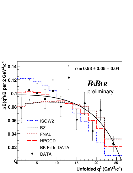
Figure 9: Differential decay rate formula (Eq. 1) fitted to the normalized partial $\mbox{$\Delta\cal B$}(q^{2})/{\cal B}$ spectrum in 12 bins of $q^{2}$. The smaller error bars are statistical only while the larger error bars include statistical and systematic uncertainties. The BK parametrization (solid black curve) reproduces the data quite well ($\chi^{2}=8.8$ for 11 degrees of freedom) with the parameter $\alpha=0.53\pm 0.05\pm 0.04$. The data are also compared to LCSR calculations [6] (dotted line), unquenched LQCD calculations [3] (long dashed line), [4] (short dashed line) and the ISGW2 quark model [7] (dash-dot line).

Table 1: $\chi^{2}$ values and associated probabilities for various QCD calculation predictions and for the ISGW2 model compared to our measured $q^{2}$ spectrum, for twelve degrees of freedom.

	stat error only		stat+syst errors
QCD calculation	$\chi^{2}$	$Prob(\chi^{2})$ (%)	$\chi^{2}$	$Prob(\chi^{2})$ (%)
ISGW2 [7]	49.5	$<$ 0.01	34.1	0.07
Ball-Zwicky [6]	17.0	14.9	13.0	37.2
FNAL [4]	16.2	18.2	12.5	41.0
HPQCD [3]	14.2	28.6	10.2	60.2

The normalized $\mbox{$\Delta\cal B$}(q^{2})/{\cal B}$ distribution is displayed in Fig. 9 together with the result of a $f^{+}(q^{2})$ shape fit using the BK parametrization and theoretical predictions. We obtain a value of $\alpha=0.53\pm 0.05\pm 0.04$. In Table 1, we give the $\chi^{2}$ values and their associated probabilities for the four different calculations. These values were obtained by comparing, bin by bin, the data with the central values of the form-factor calculations, ignoring the theoretical errors. Our experimental data are clearly incompatible with the ISGW2 quark model. A more definitive choice among the remaining theoretical calculations must await a substantial increase in statistics.

Monte Carlo studies have shown that there is no significant fit bias for the ${{\cal B}}(B^{0}\rightarrow\pi^{-}\ell^{+}\nu)$ but a small 3.8% bias in the $f^{+}(q^{2})$ parameter $\alpha$ which has been incorporated in its systematic error. Various cross-checks have also been performed. The results were obtained separately for the electron and muon decay channels, for the off-resonance data replacing the continuum PDF, for the different $\Delta E$-$m_{\rm ES}$ and $\tilde{q}^{2}$ binnings, and for the variations of all the analysis cuts, one at a time. All the cross-check studies were found to be consistent with the final results.

We extract $|V_{ub}|$ from the partial branching fractions $\Delta\cal B$ using $|V_{ub}|=\sqrt{\mbox{$\Delta\cal B$}/(\tau_{B}^{0}\Delta\zeta)}$, where $\tau_{B}^{0}=(1.536\pm 0.014)$ ps [2] is the $B^{0}$ lifetime and $\Delta\zeta=\Delta\Gamma/|V_{ub}|^{2}$ is the normalized partial decay rate predicted by various form factor calculations. We use the LCSR calculations for $q^{2}<16$ ${\mathrm{\,Ge\kern-1.00006ptV^{2}\!/}c^{4}}$ and the LQCD calculations for $q^{2}>16$ ${\mathrm{\,Ge\kern-1.00006ptV^{2}\!/}c^{4}}$. The results are shown in Table 2. The uncertainties of the form-factor normalization are taken from Refs. [3, 4, 5, 6]. We obtain values of $|V_{ub}|$ ranging from $3.6\times 10^{-3}$ to $4.1\times 10^{-3}$. For the most recently published unquenched LQCD calculation [3], we obtain $|V_{ub}|=\left(4.1\pm 0.2_{stat}\pm 0.2_{syst}{}^{+0.6}_{-0.4}{}_{\mathrm{FF}}\right)\times{10^{-3}}$.

Table 2: Values of $|V_{ub}|$ derived from the form-factor calculations. The first two errors arise from the statistical and systematic uncertainties of the partial branching fractions. The third error comes from the uncertainties on $\Delta\zeta$ due to the theoretical calculations.

	$q^{2}$ (${\mathrm{\,Ge\kern-1.00006ptV^{2}\!/}c^{4}}$)	$\Delta\cal B$ ($10^{-4}$)	$\Delta\zeta$ ($ps^{-1}$)	$|V_{ub}|$ ($10^{-3}$)
Ball-Zwicky [6]	$<16$	$1.07~{}\pm~{}0.06~{}\pm~{}0.08$	$5.44~{}\pm~{}1.43$	$3.6~{}\pm~{}0.1~{}\pm~{}0.1~{}{}^{+0.6}_{-0.4}$
HPQCD [3]	$>16$	$0.37~{}\pm~{}0.04~{}\pm~{}0.03$	$1.46~{}\pm~{}0.35$	$4.1~{}\pm~{}0.2~{}\pm~{}0.2~{}{}^{+0.6}_{-0.4}$
FNAL [4]	$>16$	$0.37~{}\pm~{}0.04~{}\pm~{}0.03$	$1.83~{}\pm~{}0.50$	$3.6~{}\pm~{}0.2~{}\pm~{}0.2~{}{}^{+0.6}_{-0.4}$
APE [5]	$>16$	$0.37~{}\pm~{}0.04~{}\pm~{}0.03$	$1.80~{}\pm~{}0.86$	$3.7~{}\pm~{}0.2~{}\pm~{}0.2~{}{}^{+1.4}_{-0.7}$

5 Summary

The succesful development of the loose neutrino reconstruction technique shows that it is not always necessary to have very pure signal samples to control the systematic errors. The gain in statistical precision can overcome the negative features of large backgrounds. This technique could thus be used advantageously in future measurements, possibly those of other exclusive $B\rightarrow X_{u}\ell\nu$ decays.

In the present analysis, we have obtained the total $B^{0}\rightarrow\pi^{-}\ell^{+}\nu$ branching fraction from the values of the partial branching fractions measured in 12 bins of $q^{2}$ and the $f^{+}(q^{2})$ shape parameter using the Becirevic-Kaidalov parametrization. We summarize these results in Table 3 together with the value of $|V_{ub}|$ extracted from a recent calculation of the form factor [3].

Table 3: Summary of the main results.

${{\cal B}}(B^{0}\rightarrow\pi^{-}\ell^{+}\nu)$ $=(1.44\pm 0.08_{stat}\pm 0.10_{syst})\times 10^{-4}$

$\alpha_{BK}=0.53\pm 0.05_{stat}\pm 0.04_{syst}$

$|V_{ub}|=\left(4.1\pm 0.2_{stat}\pm 0.2_{syst}{}^{+0.6}_{-0.4}{}_{\mathrm{FF}}\right)\times 10^{-3}$

Our value for the ${{\cal B}}(B^{0}\rightarrow\pi^{-}\ell^{+}\nu)$ is the most precise measurement to date and, by itself, is of comparable precision to the current world average [28]: ${{\cal B}}(B^{0}\rightarrow\pi^{-}\ell^{+}\nu)$ $=(1.34\pm 0.08_{stat}\pm 0.08_{syst})\times 10^{-4}$. The new value of the BK parameter is an improvement over our previous measurement $\alpha=0.61\pm 0.09$ [15] (no systematic error quoted).

The errors in Table A-2 together with the correlation matrices of the statistical and systematic errors presented in Tables A-3 and A-4 will allow the present data to be studied with different future $f^{+}(q^{2})$ parametrizations. A simple $\chi^{2}$ calculation already shows that our data are incompatible with the predictions of the ISGW2 quark model.

6 Acknowledgements

We are grateful for the extraordinary contributions of our PEP-II colleagues in achieving the excellent luminosity and machine conditions that have made this work possible. The success of this project also relies critically on the expertise and dedication of the computing organizations that support BABAR. The collaborating institutions wish to thank SLAC for its support and the kind hospitality extended to them. This work is supported by the US Department of Energy and National Science Foundation, the Natural Sciences and Engineering Research Council (Canada), Institute of High Energy Physics (China), the Commissariat à l’Energie Atomique and Institut National de Physique Nucléaire et de Physique des Particules (France), the Bundesministerium für Bildung und Forschung and Deutsche Forschungsgemeinschaft (Germany), the Istituto Nazionale di Fisica Nucleare (Italy), the Foundation for Fundamental Research on Matter (The Netherlands), the Research Council of Norway, the Ministry of Science and Technology of the Russian Federation, and the Particle Physics and Astronomy Research Council (United Kingdom). Individuals have received support from the Marie-Curie IEF program (European Union) and the A. P. Sloan Foundation.

Appendix A

The values of the partial $\Delta{{\cal B}}(B^{0}\rightarrow\pi^{-}\ell^{+}\nu,q^{2})$ and total ${{\cal B}}(B^{0}\rightarrow\pi^{-}\ell^{+}\nu)$ branching fractions are given in Table A-1, those of the normalized partial $\mbox{$\Delta\cal B$}(q^{2})/{\cal B}$ branching fractions are listed in Table A-2. All the statistical and systematic uncertainties as well as their associated correlation matrices are given in Tables A-1, A-2, A-3 and A-4.

Table A-1: Partial $\Delta{{\cal B}}(B^{0}\rightarrow\pi^{-}\ell^{+}\nu,q^{2})$ and total ${{\cal B}}(B^{0}\rightarrow\pi^{-}\ell^{+}\nu)$ $(\times 10^{7})$ and their errors $(\times 10^{7})$ from all sources.

$q^{2}$ intervals (${\mathrm{\,Ge\kern-0.90005ptV^{2}\!/}c^{4}}$)	0-2	2-4	4-6	6-8	8-10	10-12	12-14	14-16	16-18	18-20	20-22	22-26.4	Total	$q^{2}$$<$16	$q^{2}$$>$16
fitted BF	113.2	151.1	144.6	131.8	149.3	115.7	177.8	87.7	122.7	63.3	107.6	78.7	1443.6	1071.2	372.4
fitted yield stat err	22.9	20.0	19.9	20.1	22.8	21.5	24.3	20.8	23.4	19.5	20.0	20.1	83.4	63.3	44.1
trk eff	14.7	1.5	6.1	3.3	3.7	3.4	4.4	4.0	2.4	4.6	1.3	4.4	40.3	39.7	4.5
$\gamma$ eff	15.2	1.0	5.3	7.0	3.3	9.0	7.3	4.3	3.2	4.0	2.8	1.9	56.9	50.9	6.7
$K^{0}_{\scriptscriptstyle L}$ eff & E	1.6	1.0	1.1	1.4	1.5	0.8	2.2	1.6	1.7	1.5	1.2	1.8	7.1	5.2	3.7
Y PID & trk eff	2.3	2.9	2.1	2.8	2.3	1.7	3.4	1.5	2.3	0.9	1.9	1.8	22.1	15.8	6.5
continuum yield	3.2	0.6	0.4	0.1	0.1	0.2	0.2	0.6	0.6	1.3	0.8	2.1	4.2	2.2	4.6
continuum $\tilde{q}^{2}$	12.9	2.3	1.8	1.2	1.5	1.3	1.1	2.0	2.2	3.6	3.9	8.4	8.8	8.8	12.4
continuum $m_{\rm ES}$	6.1	0.6	0.4	0.1	0.9	0.6	0.1	0.7	0.5	1.1	1.2	2.0	12.4	7.7	4.7
continuum $\Delta E$	2.6	2.2	0.6	1.4	2.4	0.5	0.4	1.0	0.7	1.4	3.4	3.3	17.8	9.2	8.6
$D\rightarrow K^{0}_{L}$ BF	8.1	6.3	8.2	3.3	3.9	4.5	3.4	4.6	5.5	4.9	4.3	4.5	51.6	34.2	17.5
$b\rightarrow c\ell\nu$ BF	3.0	2.6	1.5	2.8	6.2	1.2	4.3	2.0	1.7	2.7	1.5	1.6	17.0	13.2	5.0
$b\rightarrow u\ell\nu$ BF	1.7	1.8	1.1	1.0	1.6	1.6	2.0	1.5	1.7	2.9	7.9	7.5	16.6	9.6	11.5
$\mathchar 28935\relax(4S)\rightarrow B^{0}\bar{B^{0}}$ BF	2.3	3.3	2.3	2.0	2.1	1.9	2.9	1.1	2.0	0.8	2.4	1.4	23.9	17.7	6.3
$B\rightarrow D^{*}\ell\nu$ FF	1.7	1.3	0.2	2.0	4.0	1.0	2.6	0.9	1.0	0.8	0.8	2.5	12.5	10.2	2.7
$B\rightarrow\rho\ell\nu$ FF	4.0	1.2	3.4	1.7	1.1	1.7	2.6	3.9	1.3	1.9	1.6	3.5	18.3	14.4	5.7
$B^{0}\rightarrow\pi^{-}\ell^{+}\nu$ FF	-1.2	-0.0	0.3	0.1	0.3	0.0	0.7	-0.3	-0.2	-1.3	1.6	4.5	4.7	0.0	4.7
signal MC stat error	1.8	2.6	2.4	2.6	2.4	2.3	2.6	1.5	1.7	1.1	1.3	1.1	5.5	5.1	2.2
B counting	1.2	1.7	1.6	1.5	1.6	1.3	2.0	1.0	1.4	0.7	1.2	0.9	15.9	11.8	4.1
total syst error	28.0	9.8	13.1	10.6	11.3	11.7	12.5	9.7	8.8	10.3	11.8	15.6	102.7	83.0	31.3
total error	36.2	22.3	23.8	22.7	25.5	24.5	27.3	23.0	25.1	22.1	23.3	25.4	132.3	104.4	54.1

Table A-2: Normalized partial $\mbox{$\Delta\cal B$}(q^{2})/{\cal B}$ ($\times 10^{3}$) and their errors ($\times 10^{3}$).

$q^{2}$ intervals (${\mathrm{\,Ge\kern-0.90005ptV^{2}\!/}c^{4}}$)	0-2	2-4	4-6	6-8	8-10	10-12	12-14	1 4-16	16-18	18-20	20-22	22-26.4
normalized partial BF	78.4	104.6	100.2	91.3	103.4	80.1	123.2	60.8	85.0	43.9	74.5	54.6
fitted yield stat err	15.9	13.9	13.8	13.9	15.8	14.9	16.8	14.4	16.2	13.5	13.9	14.0
signal MC stat error	1.3	1.8	1.6	1.8	1.7	1.6	1.8	1.0	1.2	0.8	0.9	0.8
track eff	7.7	2.3	1.6	0.8	1.0	0.6	1.0	1.2	2.2	2.1	2.3	4.3
photon eff	7.0	3.4	0.7	2.1	1.9	3.0	1.0	0.8	1.6	1.2	4.1	1.8
$K^{0}_{\scriptscriptstyle L}$ eff & E	0.9	0.9	0.6	0.9	0.9	0.4	1.4	1.1	1.0	1.0	0.6	1.2
Y PID & trk eff	2.3	0.5	0.2	0.7	0.3	0.1	0.7	0.2	0.4	0.5	0.2	0.5
continuum yield	2.3	0.3	0.2	0.2	0.3	0.1	0.4	0.3	0.2	0.8	0.4	1.4
continuum $\tilde{q}^{2}$	8.9	2.1	1.6	1.1	0.6	1.3	0.7	1.4	1.1	2.3	2.3	5.8
continuum $m_{\rm ES}$	3.4	0.4	0.5	0.7	1.4	0.2	1.0	0.2	0.4	0.4	0.2	0.9
continuum $\Delta E$	0.9	0.3	0.8	0.2	0.5	1.3	1.8	0.2	0.7	0.5	1.5	1.6
$\cal B$($D\rightarrow K^{0}_{L}$)	2.9	3.3	2.3	1.9	2.2	2.6	3.2	2.5	1.5	2.3	1.3	1.3
$\cal B$($b\rightarrow c\ell\nu$)	1.5	2.8	1.4	1.3	3.3	1.0	2.1	1.3	1.1	1.6	1.0	0.8
$\cal B$($b\rightarrow u\ell\nu$)	0.6	1.3	0.6	0.9	1.2	0.7	1.7	0.6	1.6	2.0	4.8	4.9
$\cal B$($\mathchar 28935\relax(4S)\rightarrow B^{0}\bar{B^{0}}$)	0.3	0.6	0.2	0.2	0.4	0.1	0.3	0.3	0.1	0.6	0.4	0.2
$B\rightarrow D^{*}\ell\nu$ FF	0.6	1.7	0.8	0.7	2.0	0.5	0.8	0.6	1.3	0.7	0.3	1.3
$B\rightarrow\rho\ell\nu$ FF	1.8	0.6	1.4	0.6	0.7	0.3	3.2	2.0	0.7	1.4	1.5	1.8
$B^{0}\rightarrow\pi^{-}\ell^{+}\nu$ FF	1.1	0.3	0.1	0.2	0.1	0.2	0.1	0.4	0.4	1.0	0.9	2.9
total syst error	15.1	7.1	4.5	4.3	5.7	4.9	6.4	4.4	4.5	5.5	7.8	10.1
total error	21.9	15.6	14.5	14.6	16.8	15.7	18.0	15.1	16.9	14.6	15.9	17.2

Table A-3: Correlation matrix of the normalized partial $\mbox{$\Delta\cal B$}(q^{2})/{\cal B}$ statistical errors.

$q^{2}$ intervals
(${\mathrm{\,Ge\kern-0.90005ptV^{2}\!/}c^{4}}$)	0-2	2-4	4-6	6-8	8-10	10-12	12-14	14-16	16-18	18-20	20-22	22-26.4
0-2	1.00	-0.20	0.12	-0.00	-0.01	0.04	0.04	-0.01	-0.00	0.01	0.01	0.01
2-4	-0.20	1.00	-0.32	0.14	0.03	0.01	0.02	-0.01	-0.00	-0.00	0.00	0.00
4-6	0.12	-0.32	1.00	-0.31	0.20	0.05	0.13	-0.02	-0.00	-0.00	0.00	0.00
6-8	-0.00	0.14	-0.31	1.00	-0.22	0.14	0.08	-0.01	-0.00	-0.00	-0.00	-0.00
8-10	-0.01	0.03	0.20	-0.22	1.00	-0.23	0.19	-0.03	0.00	-0.00	-0.00	-0.01
10-12	0.04	0.01	0.05	0.14	-0.23	1.00	-0.02	0.02	-0.00	0.00	-0.00	0.00
12-14	0.04	0.02	0.13	0.08	0.19	-0.02	1.00	-0.24	0.01	-0.02	-0.00	-0.00
14-16	-0.01	-0.01	-0.02	-0.01	-0.03	0.02	-0.24	1.00	0.00	0.11	-0.03	-0.00
16-18	-0.00	-0.00	-0.00	-0.00	0.00	-0.00	0.01	0.00	1.00	0.01	-0.04	-0.01
18-20	0.01	-0.00	-0.00	-0.00	-0.00	0.00	-0.02	0.11	0.01	1.00	-0.18	-0.11
20-22	0.01	0.00	0.00	-0.00	-0.00	-0.00	-0.00	-0.03	-0.04	-0.18	1.00	-0.01
22-26.4	0.01	0.00	0.00	-0.00	-0.01	0.00	-0.00	-0.00	-0.01	-0.11	-0.01	1.00

Table A-4: Correlation matrix of the normalized partial $\mbox{$\Delta\cal B$}(q^{2})/{\cal B}$ systematic errors.

$q^{2}$ intervals
(${\mathrm{\,Ge\kern-0.90005ptV^{2}\!/}c^{4}}$)	0-2	2-4	4-6	6-8	8-10	10-12	12-14	14-16	16-18	18-20	20-22	22-26.4
0-2	1.00	-0.58	0.04	-0.20	-0.27	0.19	-0.21	0.12	-0.48	0.15	-0.40	-0.48
2-4	-0.58	1.00	0.09	-0.16	-0.01	-0.35	0.12	-0.16	0.38	-0.39	0.34	0.16
4-6	0.04	0.09	1.00	-0.02	-0.26	0.16	-0.25	0.12	0.06	-0.05	-0.28	-0.15
6-8	-0.20	-0.16	-0.02	1.00	0.28	0.46	0.33	-0.05	-0.03	-0.20	-0.37	-0.11
8-10	-0.27	-0.01	-0.26	0.28	1.00	-0.38	0.52	-0.35	0.01	-0.33	0.15	-0.06
10-12	0.19	-0.35	0.16	0.46	-0.38	1.00	0.03	0.33	-0.22	0.14	-0.53	-0.28
12-14	-0.21	0.12	-0.25	0.33	0.52	0.03	1.00	-0.53	0.12	-0.34	0.03	-0.35
14-16	0.12	-0.16	0.12	-0.05	-0.35	0.33	-0.53	1.00	-0.33	0.36	-0.17	-0.10
16-18	-0.48	0.38	0.06	-0.03	0.01	-0.22	0.12	-0.33	1.00	0.07	0.12	0.04
18-20	0.15	-0.39	-0.05	-0.20	-0.33	0.14	-0.34	0.36	0.07	1.00	-0.29	-0.04
20-22	-0.40	0.34	-0.28	-0.37	0.15	-0.53	0.03	-0.17	0.12	-0.29	1.00	0.17
22-26.4	-0.48	0.16	-0.15	-0.11	-0.06	-0.28	-0.35	-0.10	0.04	-0.04	0.17	1.00

References

- [1] M. Kobayashi and T. Maskawa, Prog. Theor. Phys. 49, 652 (1973).
- [2] Particle Data Group, S. Eidelman et al., Phys. Lett. B 592, 1 2004.
- [3] HPQCD Collaboration, E. Gulez et al., Phys. Rev. D73, 074502 (2006).
- [4] FNAL Collaboration, M. Okamoto et al., Nucl. Phys. Proc. Suppl. 140 461 (2005).
- [5] A. Abada et al., Nucl. Phys. B619, 565 (2001).
- [6] P. Ball, R. Zwicky, Phys. Rev. D71, 014015 (2005).
- [7] D. Scora, N. Isgur, Phys. Rev. D52, 2783 (1995).
- [8] D. Becirevic and A. B. Kaidalov, Phys. Lett. B478, 417 (2000).
- [9] BABAR Collaboration, B. Aubert et al., Nucl. Instrum. Methods A479, 1 (2002).
- [10] GEANT4 Collaboration, S. Agostinelli et al., Nucl. Instrum. Methods A506, 250 (2003).
- [11] D. J. Lange, Nucl. Instrum. Meth. A462, 152 (2001).
- [12] D. Côté et al., Eur. Phys. J. C 38, 105 (2004).
- [13] CLEO collaboration, J.P. Alexander et al., Phys. Rev. Lett. 77, 25 (1996).
- [14] CLEO collaboration, S.B. Athar et al, Phys. Rev. D68, 072003 (2003).
- [15] BABAR Collaboration, B. Aubert et al., Phys. Rev. D72 051102 (2005).
- [16] BABAR Collaboration, B. Aubert et al., SLAC-PUB-11966, Submitted to Phys. Rev. Lett.
- [17] Belle Collaboration, T. Hokuue et al., hep-ex/0604024, Submitted to Phys. Lett. B.
- [18] M. S. Gill, Ph.D. Thesis, University of California, Berkeley (UCB) (2004) [SLAC Report 794: http://www.slac.stanford.edu/pubs/slacreports/slac-r-794.html]
- [19] BABAR Collaboration, B. Aubert et al., hep-ex/0602023, Submitted to Phys. Rev. D.
- [20] W. D. Hulsbergen, Nucl. Instrum. Meth. A552, 566 (2005).
- [21] G.C. Fox and S. Wolfram, Phys. Rev. Lett. 41, 1581 (1978).
- [22] BABAR Collaboration, B. Aubert et al., Phys. Rev. D67, 031101 (2003).
- [23] F. J. Gilman, R. L. Singleton, Phys. Rev. D41, 142 (1990).
- [24] R. J. Barlow and C. Beeston, Comput. Phys. Commun. 77, 219 (1993).
- [25] R. Hill, Phys. Rev. D73, 014012 (2006)
- [26] P. Ball, R. Zwicky, Phys. Lett. B625, 225 (2005)
- [27] P. Ball, R. Zwicky, Phys. Rev. D71, 014029 (2005).
- [28] http://www.slac.stanford.edu/xorg/hfag/semi/winter06/winter06.shtml