CDF Collaboration
Measurement of the Production Cross Section in collisions at = 1.96 TeV using Lepton+Jets Events with Jet Probability b-tagging
Abstract
We present a measurement of the production cross section using events with one charged lepton and jets from collisions at a center-of-mass energy of 1.96 . A -tagging algorithm based on the probability of displaced tracks coming from the event interaction vertex is applied to identify quarks from top decay. Using 318 of data collected with the CDF II detector, we measure the production cross section in events with at least one restrictive (tight) -tagged jet and obtain (stat.)(syst.) . The cross section value assumes a top quark mass of in the acceptance corrections. The dependence of the cross section on is presented in the paper. This result is consistent with other CDF measurements of the cross section using different samples and analysis techniques, and has similar systematic uncertainties. We have also performed consistency checks by using the -tagging probability function to vary the signal to background ratio and also using events that have at least two -tagged jets.
pacs:
14.65.Ha, 13.85.Ni, 13.85.QkI
The top quark is the most massive fundamental particle observed so far, and the study of its properties is interesting for several reasons ranging from its possible special role in electroweak symmetry breaking to its sensitivity to physics beyond the standard model (SM). In particular, the measurement of the top quark pair production cross section is of interest as a test of QCD predictions. Recent QCD calculations done with perturbation theory to next-to-leading order predict with an uncertainty of less than 15% bib:ref1 ; bib:ref11 , which motivate measurements of comparable precision.
Top quark pairs in the SM are produced via either quark-antiquark annihilation or gluon-gluon fusion in hadron colliders. At the Fermilab Tevatron collider, with a center-of-mass energy of 1.96 in collisions, about 85% of the total top pair production comes from quark-antiquark annihilation. At this center-of-mass energy, the calculated cross section, for the combined Tevatron Run I top mass of 178 bib:runimass , is 6.1 bib:ref1 and decreases by approximately 0.2 for each increase of 1 in the value of the top mass over the range . The standard model top quark decays to a boson and a quark almost 100% of the time, resulting in a final state from production of two bosons and two jets from quark fragmentation. When one decays leptonically and the other decays to quarks, the event typically contains a high momentum charged lepton, an undetected neutrino and four high transverse momentum jets, two of which originate from quarks. The undetected neutrino results in an imbalance of the transverse energy of the event, labeled as “missing ” (). This decay mode is called “lepton+jets”.
In this paper, we report a measurement of the cross section for pair production of top quarks in the lepton+jets channel in 318 pb-1 of collision data at = 1.96 . The data were recorded between March 2002 and August 2004, during Run II of the Tevatron, by the CDF II detector, a general purpose detector which combines charged particle trackers, sampling calorimeters, and muon detectors. Processes in which a boson is produced in association with several jets with large transverse momentum can be misidentified as , since they have the same signature. In order to separate the events from this background, we develop a method to tag -jets based on tracking information from the silicon detector. The main event selection requires at least one tight (more restrictive) tag in the event. As a cross check, we also measure the cross section using events with a loose (less restrictive) tag and events which have at least two tight or at least two loose tags. Background contributions from heavy flavor production processes, such as , or , misidentified bosons, electroweak processes, single top production, and mistagged jets are estimated using a combination of Monte Carlo calculations and independent measurements in control data samples. An excess over background in the number of events that contain a lepton, missing energy and three or more jets with at least one -tag is assumed to be a signal of production and is used to measure the production cross section .
Previous measurements bib:ref2 at TeV gave a production cross section consistent with the standard model prediction. Recent CDF measurements at TeV are reported in Refs. bib:dilepton ; bib:bkin ; bib:secvtx ; bib:slt ; bib:kin and use different techniques and top decay channels. The measurement described here analyzes more data than the above, and uses a jet probability -tagging algorithm. A feature of this algorithm is that -tagging is based on a continuous probability function rather than on a discrete object such as a secondary vertex. Potentially, this tagger can also be used to statistically separate and heavy flavor contributions.
The organization of this paper is as follows. Section II reviews the detector systems relevant to this analysis. In Section III, we describe the data sample and event reconstruction. The -tagging algorithm and its efficiency and misidentification (“fake”) rate are discussed in Section IV. Section V describes the event selection. The estimate of the different backgrounds is presented in Section VI. The event acceptance and tagging efficiency are derived in Section VII. The production cross section measurements in single and double tagged events are reported in Sections VIII, and IX, respectively. Finally, the conclusions are presented in Section X.
II The CDF II Detector
The CDF II detector uses a cylindrical coordinate system with the coordinate along the proton direction, the azimuthal angle , and the polar angle usually expressed in terms of the pseudo-rapidity = -ln[tan(/2)]. The rectangular coordinates and point radially outward and vertically upward from the Tevatron ring, respectively. The detector has been described in detail elsewhere bib:cdf_det . In this section, we give a brief description of the parts relevant for the analysis.
Tracking systems are essential to trigger on and identify high momentum charged particles such as electrons and muons. The charged particle tracking detectors are contained in a superconducting solenoid which generates a magnetic field of 1.4 , oriented parallel to the proton beam direction. The Central Outer Tracker (COT) bib:cdf_cot is a 3.1 long open cell drift chamber which performs up to 96 track position measurements in the region between 0.40 and 1.37 from the beam axis. Sense wires are arranged in 8 alternating axial and 2∘ stereo superlayers with 12 wires each. The position resolution of a single drift time measurement is approximately 140 . For high momentum tracks, the COT transverse momentum resolution is .
Inside the inner radius of the COT, a five layer doubled-sided silicon microstrip detector (SVX) bib:cdf_svx2 covers the region between 2.5 to 11 from the beam axis. Three separate SVX barrel modules along the beamline cover a length of 96 , approximately 90% of the luminous beam intersection region. Three of the five layers combine an - measurement on one side and a 90∘ stereo measurement on the other, and the remaining two layers combine - with a small stereo angle of 1.2∘. Silicon microstrips have a pitch of 60 to 65 depending on the layer. Three additional Intermediate Silicon Layers (ISL) bib:isl at radii between 19 and 30 in the central region link tracks in the COT to hits in SVX.
Electromagnetic (EM) and hadronic (HAD) sampling calorimeters bib:cem ; bib:pem ; bib:chad surround the tracking system and measure the energy flow of interacting particles in the pseudo-rapidity range 3.64. The EM and HAD calorimeters are lead-scintillator and iron-scintillator sampling devices, respectively. They are segmented into projective towers, each one covering a small range in pseudo-rapidity and azimuth. Most towers cover 15 degrees in and 0.10 to 0.13 units in pseudo-rapidity. Proportional chambers (CES) measure the transverse profile of EM showers at a depth corresponding to the shower maximum for electrons. Electrons are reconstructed in the central electromagnetic calorimeter (CEM) with a transverse energy precision bib:cem . Jets are identified as a group of electromagnetic and hadronic calorimeter towers with an energy resolution of approximately 0.1 + 1.0 bib:jet_e_res .
The muon system is located outside of the calorimeters. Four layers of planar drift chambers (CMU) bib:cmu detect muons with that penetrate the five absorption lengths of calorimeter steel in the central region of 0.6. An additional four layers of planar drift chambers (CMP) bib:cmp located behind 0.6 of steel outside the magnet return yoke detect muons with . When a track is linked to both CMU and CMP, it is called a CMUP muon. The Central Muon Extension detector (CMX), arranged in a conical geometry, provides muon detection in the region 0.6 1.0 with four to eight layers of drift chambers, depending on the polar angle. All the muon chambers measure the azimuthal coordinates of hits via a drift time measurement. The CMU and CMX also measure the longitudinal coordinate, .
The beam luminosity is determined by using gas Cherenkov counters bib:lumi located in the region 3.7 4.7 which measure the average number of inelastic collisions per bunch crossing. The total uncertainty on the luminosity is 5.9%, where 4.4% comes from the acceptance and operation of the luminosity monitor and 4.0% from the calculation of the inelastic cross section bib:lumi_sys .
III Data Sample and Event Reconstruction
The data used in this analysis are from collisions at a center-of-mass energy of 1.96 recorded by the CDF II detector between March 2002 and September 2004. The data sample has been collected by triggers based on the selection of a high transverse momentum lepton (electron or muon). The total integrated luminosity is 318 for CEM electron and CMUP muon candidates, and 305 for CMX muon candidates. Briefly, we discuss the trigger and lepton identification requirements, the reconstruction of jets, and the missing transverse energy, .
CDF has a three-level trigger system to filter events from a 2.5 beam crossing rate down to 60 for permanent storage. The first two levels of triggers are special purpose hardware and the third consists of a farm of computers.
The first trigger level (L1) reconstructs charged particle tracks in the COT - projection using a hardware track processor called the Extremely Fast Tracker (XFT) bib:xft . The L1 electron trigger requires a XFT track with 8 matched to an EM calorimeter tower with 8 and with a ratio of hadronic-to-electromagnetic energy less than 0.125. The L1 muon trigger requires an XFT track with 4 matched to a muon track segment with 6 from the CMU and CMP chambers or a track with matched to a muon track segment with 6 in the CMX chambers.
The second level (L2) electron trigger requires the XFT track found at L1 to be matched to a cluster of energy in the central EM calorimeter with 16 . The cluster adds the energy of the neighboring trigger towers with 7.5 to the original L1 trigger tower. A trigger tower consists of two calorimeter towers. The L2 muon trigger accepts events passing L1.
The third trigger level (L3) is a farm of Linux computers which perform on-line event reconstruction, including 3D charged particle reconstruction. The L3 electron trigger requires a track with 9 matched to an energy cluster of three adjacent towers in pseudo-rapidity in the central EM calorimeter with 18 , consistent with the shower profile expected from test beam electrons. The L3 muon trigger requires a track with 18 matched to a track segment in the muon chambers within 10 in the view and, for CMU and CMX muons only, within 20 in the view. The efficiency of these triggers is measured using and data (the method is described in Ref. bib:eff_tri ) and is found to be (96.2 0.6)% for CEM electrons, and (90.8 0.5)% and (96.5 0.4)% for CMUP and CMX muons respectively, for electrons and muons passing through the fiducial volume of these detectors.
III.1 Track and Primary Vertex Reconstruction
The trajectories of charged particles are found (in a first approximation) as a series of segments in the axial superlayers of the COT. Two complementary algorithms associate the segments lying on a common circle to define an axial track. Segments in the stereo layers are associated with the axial tracks to reconstruct 3D tracks. For muons and electrons used in this analysis, COT tracks are required to have at least 3 axial and 2 stereo segments with at least 5 hits per superlayer. The efficiency for finding isolated high momentum COT tracks in the COT fiducial volume with 10 is measured using electrons from events and is found to be (98.3 0.1)%. Silicon hit information is added to reconstructed COT tracks using an “outside-in” tracking algorithm. The COT tracks are extrapolated to the silicon detector and the track is refit using the information from the silicon measurements. The initial track parameters provide a width for a search region in a given layer. For each candidate hit in that layer, the track is refit and used to define the search region into the next layer. The search uses the two best candidate hits in each layer to generate a small tree of final track candidates, and the one with the best fit is selected. The efficiency to associate at least three silicon hits with an isolated COT track is found to be (91 1)%.
The primary vertex location for a given event is found by fitting well-measured tracks to a common point of origin. At high luminosities, more than one collision can occur on a given bunch crossing. For a luminosity of 10s-1, there are 2.3 interactions per bunch crossing. The luminous region is long, with = 29 ; therefore the primary vertices of each collision are typically separate in . The first estimate of the primary vertices (, , ) is binned in the coordinate, and the position of each vertex is then calculated from the weighted average of the coordinate of all tracks within 1 of the first iteration vertex, with a typical resolution of 100 m. The primary vertex is determined event by event by an iterative algorithm which uses tracks around a seed vertex, defined as above, to form a new vertex. The for all tracks relative to the new vertex is calculated, tracks with bad are removed, and the cycle is repeated until all tracks have a good . The locus of all primary vertices defines the beamline, the position of the luminous region of the beam-beam collisions through the detector. A linear fit to (, ) vs. yields the beamline for each stable running period. The beamline is used as a constraint to refine the knowledge of the primary vertex in a given event. The transverse beam cross section is circular, with a rms width of at = 0, rising to 50 - 60 at = 40 . The beam is not necessarily parallel nor centered in the detector.
III.2 Electron Identification
Electron reconstruction begins with a track with that extrapolates to a cluster of three CEM towers adjacent in pseudo-rapidity with a total . Several cuts are successively applied in order to improve the purity of the electron selection, as summarized in Table 1. Electron candidates passing these requirements are called tight electrons.
| Electron Variable | Cut |
|---|---|
| COT Axial Segments | |
| COT Stereo Segments | |
| Hits for Each COT Segment | |
| unless | |
| Isolation | |
| CES | |
| CES | |
| CES | |
| Photon Conversions | Veto if and |
The ratios between the hadronic and the electromagnetic cluster energies and between the cluster energy and the track momentum are required to be consistent with an electron’s energy deposition in the calorimeters. The cluster is further required to be isolated, the isolation being defined as the ratio of the additional transverse energy in a cone of radius around the cluster to the transverse energy of the cluster itself.
The position of the electromagnetic shower measured by the CES detector is used to define matching requirements between the extrapolated track and the cluster in the CES and local coordinates. In particular, a charge dependent cut in the position is applied to take into account the different flow of energy deposited by bremsstrahlung photons emitted by an electron or a positron. In addition, the CES provides electron identification through the observed shower shape. The CES shower shape is fitted in the z view to the distribution expected for an electron, and the chisquare probability for the fit, , is used as a cut on the shower profile. Finally, the sharing of energy between adjacent calorimeter towers is quantified by the lateral shower profile , which measures how close the energy distribution in the CEM towers adjacent to the cluster seed is to the electron hypothesis.
Electrons from photon conversions throughout the detector material are vetoed by rejecting electron candidates if an oppositely charged track with a small distance of closest approach () is found. This analysis is sensitive to any loss in efficiency from the misidentification of an electron from the boson decay as a photon conversion. Therefore, in order to avoid loss of efficiency, the veto is not applied to events consistent with electrons radiating a photon that subsequently converts. The performance of this algorithm to identify electrons from photon conversions is estimated to be (72.6 0.1)% bib:kin , where the uncertainty covers both statistical and systematic.
The efficiency of the electron selection on events is determined by means of Monte Carlo simulation. Studies of processes show that a data to Monte Carlo simulation scale factor of (99.6 )% is needed to correct the simulation predictions for the efficiency for CEM electron identification.
Other electron categories are defined. Candidate electrons passing all the above requirements except for the isolation cut are called loose electrons. Tracks matched to an energy deposit in the plug calorimeter () are called plug electrons.
III.3 Muon Identification
Muon identification starts by requiring an isolated, high momentum COT track that extrapolates to a track segment in the muon chambers. Several additional requirements are imposed in order to minimize contamination from hadrons punching through the calorimeter, decays in flight of charged hadrons and cosmic rays. Table 2 lists the selection requirements for candidate muons. Muon candidates passing these cuts are called tight muons.
| Muon Variable | Cut |
|---|---|
| COT Axial Segments | |
| COT Stereo Segments | |
| Hits for Each COT Segment | |
| if no silicon hits | |
| if silicon hits | |
| max | |
| max | |
| CMU | |
| CMP | |
| CMX | |
| Isolation | |
| Cosmic Rays | Veto |
The COT track must have , and at least 3 axial and 2 stereo segments with a minimum of 5 hits per segment. The distance of closest approach of the track to the beamline in the transverse plane, , must be small in order to select prompt muons (coming from the interaction primary vertex) and reject cosmics and in-flight decays. The energy deposition in the EM and HAD calorimeters, and , must be small as expected for the passage of a minimum ionizing particle. The distance between the extrapolated COT track and the track segment in the muon chambers, , must be small in order to ensure a good match. If a track is matched to a CMU segment, a matching CMP segment is also required, and vice versa. Isolation is defined as the ratio between any additional transverse energy in a cone of radius around the track direction and the muon , and it is required to be smaller than 0.1. Cosmic rays are efficiently identified and rejected through their asynchronous track timing relative to the beam crossing time and their incoming and outgoing back-to-back track topology.
Studies of processes show that a data to Monte Carlo simulation scale factor of (87.4 0.9)% ((98.9 0.6)%) is needed to correct the simulation predictions for the CMUP (CMX) muon identification efficiency.
As for the electrons, candidate muons passing all the cuts except the isolation cut are called loose muons. A track matched to a CMU or a CMP segment only, which passes all the other cuts including isolation, is also accepted as a loose muon.
III.4 Jet Reconstruction and Corrections
The jets used in this analysis are reconstructed from calorimeter towers using a cone algorithm bib:jet_rec with a radius 0.4, for which the of each tower is calculated with respect to the coordinate of the event. The calorimeter towers belonging to any electron candidate are not used by the jet clustering algorithm. The energy of the jets is corrected bib:jet_e_corr for the pseudo-rapidity dependence of the calorimeter response, the calorimeter time dependence, and extra from any multiple interactions.
By definition, tight jets have corrected 15 and detector 2.0, whereas loose jets have corrected 8 and detector 2.0. Detector is the pseudo-rapidity of the jet calculated with respect to the center of the detector.
III.5 Missing Transverse Energy Reconstruction
The presence of neutrinos in an event is inferred by an imbalance of transverse energy in the detector. The missing transverse energy, , is defined as the magnitude of , where is the transverse energy of the calorimeter tower calculated with respect to the coordinate of the event, is its azimuthal angle, and the sum is over all calorimeter towers. The is corrected by subtracting the transverse momentum of the muon track and adding back the transverse energy in the calorimeter towers traversed by the muon. Because the calculation uses all calorimeter towers, the vector is adjusted for the effect of the jet corrections for all jets with 8 and 2.5.
III.6 Monte Carlo Samples and Detector Simulation
The understanding of acceptances, efficiencies and backgrounds relies on detailed simulation of physics processes and detector response.
The detector acceptance for events is modeled using PYTHIA v6.2 bib:pythia and HERWIG v6.4 bib:herwig . This analysis uses the former for the final cross section estimate and the latter to estimate the systematics due to differences in the modeling of production and decay. These generators employ leading order matrix elements for the hard parton scattering, followed by parton showering to simulate gluon radiation and fragmentation effects. The generators are used with the CTEQ5L parton distribution functions bib:cteq5l . Decays of and hadrons are modeled using QQ v9.1 bib:qqv9.1 . Estimates of backgrounds from bosons produced in association with jets are derived using the ALPGEN generator bib:alpgen with parton showering provided by HERWIG. The background from electroweak processes and single top production is studied using PYTHIA.
The CDF II detector simulation reproduces the response of the detector and uses the same detector geometry database as the event reconstruction. Particle interactions through matter are performed with GEANT3 bib:geant3 . Charge deposition in the silicon detectors is calculated using a simple geometrical model based on the path length of the ionizing particle and an unrestricted Landau distribution. The drift model for the COT uses a parametrization of a GARFIELD bib:garfield simulation with parameters tuned to match COT collider data bib:cdf_cot . The calorimeter simulation uses the GFLASH bib:gflash parametrization package interfaced with GEANT3. The GFLASH parameters are tuned to test beam data for electrons and high- pions and they are checked by comparing the calorimeter energy of isolated tracks in collision data to their momentum as measured in the COT. More details on the CDF II simulation can be found in Ref. bib:cdf_sim .
IV Jet Probability -Tagging Algorithm
The jet probability -tagging algorithm bib:jet_probab is used to determine whether a jet has been produced from the hadronization process of a light parton or a heavy parton. The latter result in long-lived hadrons whose decay gives rise to tracks displaced from the primary interaction vertex. This algorithm uses tracks associated with a jet to determine the probability for these to come from the primary vertex of the interaction. The calculation of the probability is based on the impact parameters () of the tracks in the jet and their uncertainties. The impact parameter is assigned a positive or negative sign depending on the position of the track’s point of closest approach to the primary vertex with respect to the jet direction, as shown in Fig. 1. By construction, the probability for tracks originating from the primary vertex is uniformly distributed from 0 to 1. For a jet coming from heavy flavor hadronization, the distribution peaks at 0, due to tracks from long lived particles that have a large impact parameter with respect to the primary vertex.
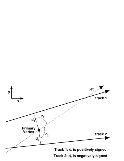
The particles in a jet coming from a light parton originate at the primary vertex, but these tracks are reconstructed with a non-zero impact parameter due to the finite tracking resolution. They have an equal probability of being positively or negatively signed. Jets which originate from a heavy parton contain long lived hadrons giving rise to tracks displaced in the jet direction, which preferentially populate the positive side of the signed impact parameter distribution. The width of the negative impact parameter distribution is solely due to the tracking detector resolution, beam spot size, and multiple scattering.
The tracking resolution can be extracted from the data by fitting the negative side of the signed impact parameter distribution of tracks from prompt jets, which are the dominant component of inclusive jet data. Tracks are divided into 72 different categories according to the number and quality of SVX hits, detector and . To minimize the contribution from badly measured tracks with a large reconstructed impact parameter, the signed impact parameter significance, (ratio of the impact parameter to its uncertainty), is parameterized for each track category. Tracks are fitted to a helix, and the impact parameter is corrected for beam offsets in order to take into account any displacement of the primary vertex from the nominal position. The uncertainty in the impact parameter is given by the error propagation of the uncertainties in the fit and in the beam offset correction. We parameterize the impact parameter significance for tracks satisfying the quality criteria listed in Table 3 that are associated with jets with and 2.5. These tracks must have , impact parameter less than 0.1 cm (in order to reject long lived ’s and ’s), three to five hits on different axial layers of the SVX, at least 20 (17) hits in the COT axial (stereo) layers, and the position of the track must be within 5 cm of the event primary vertex. Tracks passing this selection are called jet probability tracks. The is measured with respect to the primary vertex. The event is required to have a primary vertex, and the vertex with highest sum of transverse momentum of all tracks is chosen in events which have more than one vertex.
| Variable | Cut |
|---|---|
| 0.1 | |
| 3 and 5 | |
| 20 | |
| 17 | |
| 5 |
Figure 2 shows the distribution of the impact parameter significance of tracks in an inclusive jet sample for one of the track categories, namely tracks with at least 5 good SVX hits, and . The negative side of this distribution is fitted with a function called the resolution function, which is
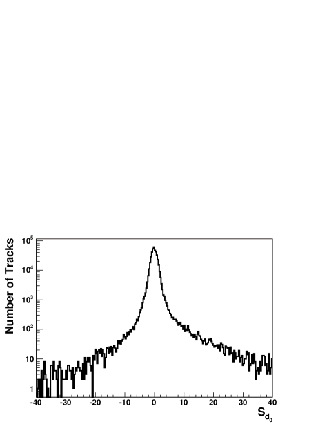
used to determine the probability, , that the impact parameter significance of a given track is due to the detector resolution, defined as:
| (1) |
The distribution peaks at zero and falls quickly with increasing absolute value of , but the tails are rather long. In order to improve the statistics and obtain a better fit in the tail, we use non-linear bins by transforming it to , where the minus sign indicates that only the negative part of is used. Figure 3 shows the result of such a fit, together with the fit residues defined as (data-fit)/uncertainty, where the uncertainty is taken as the statistical uncertainty on each data point.
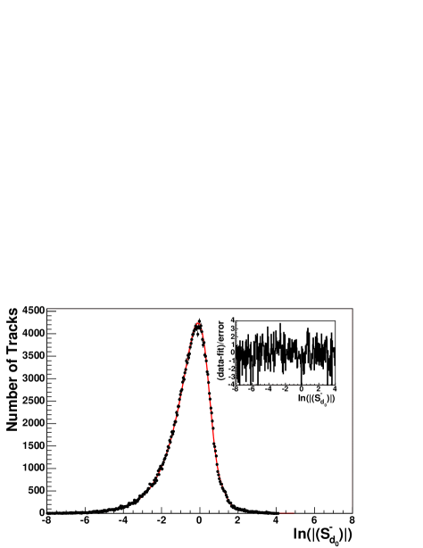
A resolution function parameterized as the convolution of four Gaussians with means at zero is found to fit well all distributions for all 72 track categories:
| (2) |
After the transformation to a logarithmic axis, the resolution function becomes
| (3) |
and is used to fit the transformed distribution.
The jet probability that a jet is consistent with a zero lifetime hypothesis is defined as
| (4) |
where
| (5) |
and is the number of jet probability tracks with positive impact parameter. Jets are required to have at least two jet probability tracks with positive impact parameter to be taggable. Both of these distributions should be uniformly distributed in the interval [0-1] for jets having only prompt tracks. Tracks with negative impact parameter are used to define a negative , which is used to check the algorithm and to estimate the misidentification rate. We define positive (negative) tagged jets as those jets whose positive (negative) is less than a cutoff, where we use 1% (main result) and 5% (cross check). Positive tagged jets are expected to be enriched in heavy flavor. The 1% cut was used in previous publications bib:jet_probab and has similar performance to the secondary vertex tagger bib:secvtx , while the loose (less restrictive) 5% cut was chosen near the point where the distribution becomes flat (see Fig. 12). Further gain in selection efficiency resulting from a looser cut is accompanied by an increase in background from light jets misidentified as heavy flavor (mistags). For comparison, both the 1% and 5% numbers and figures are presented together throughout the paper.
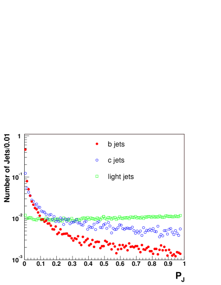
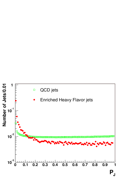
A feature of this algorithm is that the -tagging is performed using a continuous variable instead of a discrete object like a reconstructed secondary vertex. It therefore provides a variable that allows one to move continuously along the efficiency curve and to select the optimal signal to background point for a specific analysis. Furthermore, the ability to adjust the cut is a valuable tool to understand the heavy flavor content of the sample. Potentially bib:jet_probab , this method can be used to statistically separate and heavy flavor contributions. This feature is illustrated in the left plot in Fig. 4, where the jet probability distributions for , and light jets are shown. Monte Carlo simulated parton events are used as described in Section IV.1. In the right plot, we show the jet probability distributions observed in two different data sets of jets. The first sample is enriched in heavy flavor content by requiring the jets to contain a soft momentum electron; here, events are triggered on low inclusive electrons (see Section IV.1). The second set consists of generic QCD jets selected by requiring events with at least one jet with (the Jet50 sample).
In this section we discuss the -tagging algorithm itself, independently of the other details of this analysis.
IV.1 Measurement of the Tagging Efficiency for Heavy Quark Jets
The method used to measure the jet probability tagging efficiency for heavy flavor jets is described in detail in Ref. bib:secvtx . The ideal events to study this efficiency are dijet events. We use a calibration data sample of jets whose heavy flavor fraction can be measured: a sample triggered on low inclusive electrons which is enriched in semileptonic decays of bottom and charm hadrons. The tagging efficiency is also measured for simulated jets by using a Monte Carlo sample similar to the calibration sample. We use HERWIG to generate 22 parton events, which are passed through a filter requiring an electron with and . Events passing this filter are processed using the detector simulation described in Section III.6. Electrons are identified using a selection similar to that described in Section III.2, except that they are required to be non-isolated and have a lower energy threshold ( and track ). The heavy flavor content of the sample is further enhanced by requiring two jets in the event, an “electron jet”, presumed to contain the decay products of a heavy flavor hadron, and an “away jet”. The electron jet must have and be within 0.4 of the electron direction in - space. The away jet is required to have and , and it must be approximately back-to-back with the electron jet ( rad). If the fraction of electron jets containing heavy flavor for which the away jet is tagged () is known, and if there were no prompt jets misidentified as -jets, the efficiency to tag a heavy flavor jet containing an electron would be given by
| (6) |
where is the number of events for which both the electron jet and the away jet are positively tagged, and is the total number of events for which the away jet is positively tagged. Since light jets can be tagged as well, we correct for this effect by subtracting the number of negative tags. We define the positive tag excess for events with a positive or negative tag in the away jet as
| (7) | |||
| (8) |
where, for example, is the number of events where the electron jet is negatively tagged and the away jet is positively tagged. The tagging efficiency for heavy flavor jets containing an electron is then given by
| (9) |
Since events with an electron jet and a tagged away jet are mostly due to heavy flavor pair production, one expects to be close to unity. This number is less than 1.0 due to events in which the away jet is mistagged or contains heavy flavor due to gluon splitting or flavor excitation, and the electron is either a jet misidentified as electron or part of a photon conversion pair. If denotes the probability to positively tag the away jet in an event where the electron jet is a light jet, then is given by
| (10) |
where denotes the total heavy flavor fraction of electron jets. Here and are the total and fractions of electron jets, respectively, and is the to fraction ratio. We estimate using identified conversions as
| (11) |
where N is the number of events passing the selection, , and the subscript refers to events where the electron was identified as a conversion. A full derivation of this expression can be found in Ref. bib:secvtx . Two methods are used to measure the -fraction, , of the electron jets. The first method is to reconstruct decays within the electron jet and use the invariant mass sidebands to subtract background. The second method involves searching for secondary muons within the electron jet resulting from cascade decays using the same-sign rate to estimate the background. The contribution from charm, , is determined from Monte Carlo simulation to be . For inclusive electron data we measure and .
The efficiencies to tag a taggable heavy flavor jet with in data are summarized in Table 4 for 1% and 5%. The ratio of data efficiency to Monte Carlo simulation efficiency is called the tagging scale factor (). The uncertainties shown are statistical and systematic, which are described below.
| 1% | 5% | |
|---|---|---|
| (Data) | 0.258 0.011 | 0.334 0.016 |
| 0.817 0.07 | 0.852 0.072 |
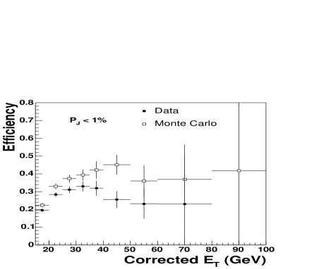
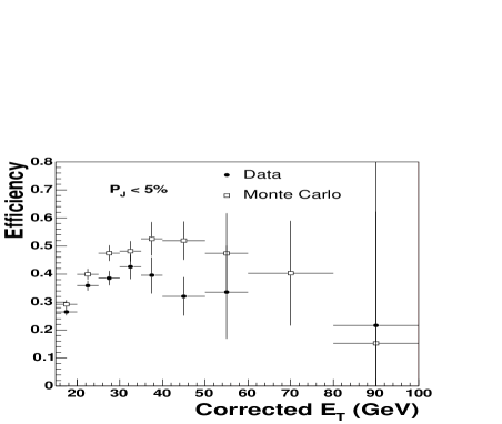

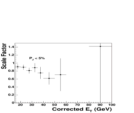
It is crucial to understand the tagging efficiency and scale factor dependences on the jet in order to characterize the jet probability algorithm performance. The dependence observed in the inclusive electron sample is shown in Fig. 5 and 6 for the tagging efficiency and scale factor respectively. Due to the lack of statistics at high jet , we repeat the study using two samples of high energy jets selected by requiring events with at least one jet with (the Jet20 sample) or with (the Jet50 sample). The absolute value of the can not be extracted because of the unknown content of heavy flavor in these samples. However, since the variations of heavy flavor fraction are relatively small over a large range of , we can still estimate the dependence of the scale factor from the dependence of the ratio of positive tag excess between data and Monte Carlo simulation.
| Sample | 1% | 5% |
|---|---|---|
| Inclusive Electron | -0.0082 0.0037 | -0.0081 0.0044 |
| Jet 20 | -0.0008 0.0019 | -0.0028 0.0024 |
| Jet 50 | 0.0005 0.0008 | 0.0005 0.0009 |
| Weighted Average | -0.00002 0.00070 | -0.00020 0.00072 |
Table 5 shows the results of a linear fit of the tagging scale factor to the jet in the inclusive electron, Jet20 and Jet50 samples. The combined estimate of the slopes is found to be consistent with a flat dependence of the scale factor both when a cut of 1% and 5% is applied. Based on these results, we conclude that the scale factor measured in the inclusive electron sample is valid at any .
Different sources of systematic uncertainty in the determination of have been considered. An uncertainty on the value of , determined from the rate of decays, comes from the branching ratio (). A factor is used to normalize the Monte Carlo simulation prediction to the PDG bib:pdg value. The uncertainty includes both the PDG branching ratio uncertainty and the Monte Carlo simulation statistical error. Another uncertainty on comes from the difference in reconstruction efficiency, , between data and Monte Carlo simulation. This uncertainty is derived by studying the efficiency of reconstruction for simulated decays embedded into data events, and is found to be 10%. There is an additional uncertainty due to the assumption of symmetry between negative tags and positive mistags implicit in the derivation of Equation 9. The effect of a mistag asymmetry is estimated by scaling the subtracted negative tags by different factors ranging from 0 to 2 (0.4 to 1.4) for 1% (5%) jet probability cuts, and an uncertainty of 7% is conservatively derived on the tagging scale factor due to this effect. Final estimates for jet probability tagging efficiencies and scale factors are summarized in Table 4.
We do not measure the tagging scale factor for jets. We assume a common scale factor for jets from and quarks and we increase the uncertainty for a quark scale factor by 100% to take into account additional uncertainties due to this assumption.
IV.2 Measurement of the Mistag Rate
An important ingredient of any analysis which uses heavy flavor tagging is the background from light quark or gluon jets incorrectly tagged as heavy flavor. The probability of (positively) tagging a light jet (the “mistag rate”) is closely related to the negative tag rate. We remind the reader that a positive (negative) is calculated using positively (negatively) signed impact parameter tracks, and a jet which has positive (negative) smaller than a certain cut is said to be positively (negatively) tagged. It is assumed that the negative tags are due to detector resolution effects only, while the positive tag rate has an additional contribution from real heavy flavor in the jets. Under this assumption, the mistag rate is equal to the negative tag rate, although in reality there is also a small contribution from heavy flavor jets to the negative tag rate and there are contributions from ’s, ’s and nuclear interactions with the detector material to the positive tag rate. These effects are considered later in Section IV.2.1.
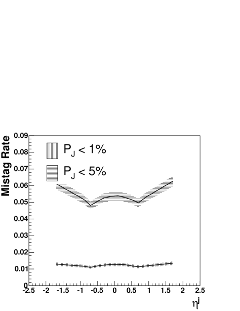
Since the tag rate has a considerable dependence on jet kinematics, it is parameterized as a 6 dimensional tag rate matrix, or look-up table, of the transverse energy of the jet, the number of jet probability tracks in the jet , the sum of the transverse energy of all jets in the event , the of the jet computed with respect to the center of the detector, the vertex position and the of the jet. The tag rates are obtained from four inclusive jet samples selected by requiring the of the most energetic jet in the event to be greater than 20, 50, 70 or 100 respectively. For a 1% (5%) cut, the overall negative tag rate is (1.22 0.08)% ((5.30 0.25)%), while the overall positive tag rate is (3.54 0.18)% ((9.20 0.26)%). Overall tag rates depend on the sample, which is why the tag rates are parameterized as a function of different variables. Figure 7 shows the negative tag rates for 1% and 5% as a function of the jet and pseudo-rapidity. The bands represent the total uncertainty.

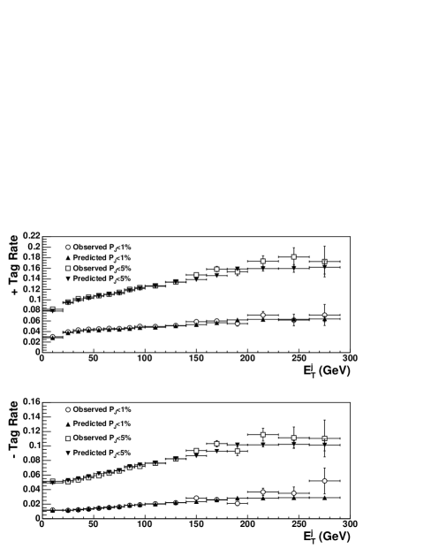
We estimate the systematic uncertainties by comparing the observed and predicted tag rates in different data samples. We apply tag rate matrices, constructed using different inclusive jet subsamples, to different datasets. Results are shown in Table 6 for a cut of 1%. The largest deviation between observed and predicted tag rates across the different jet samples is taken as the systematic uncertainty due to the sample dependence of the matrix. In order to account for any possible bias due to the trigger selection, we apply the matrix separately to trigger and non-trigger jets. A trigger jet is defined as the jet closest in - space to the level 2 cluster that fired the trigger. We also apply a matrix built with a high statistics sample of Jet20 events, to the Jet50 sample which has several jets below the trigger threshold of 50 . Also considered is a sample selected by requiring at least four jets with and . These events are expected to give a reasonable estimate of the systematic uncertainty because of the higher jet and track multiplicities. Furthermore, this sample is not used to build the matrix, making it sensitive to any additional sources of systematic uncertainty. Figure 8 compares the observed and predicted tag rates in the sample as a function of jet . The total systematic uncertainty on the overall tag rates is conservatively taken as the sum in quadrature of the , Jet20 to Jet50, and the largest of the trigger and sample contributions. Table 7 summarizes the relative uncertainties on the overall tag rates for cuts of 1% and 5%. The total relative uncertainty is 5.0% (2.8%) for positive tag rate and 6.7% (4.7%) for negative tag rate for a cut of 1% (5%).
| Matrix | Sample | Obs./Pred. Pos. Tag Rate Ratio | Obs./Pred. Neg. Tag Rate Ratio |
|---|---|---|---|
| Inc. Jet Even | Inc. Jet Odd | 0.9970.002 | 0.9990.003 |
| Inc. Jet Even | Jet20 Odd | 0.9870.003 | 0.9700.006 |
| Inc. Jet Even | Jet50 Odd | 0.9910.003 | 0.9980.006 |
| Inc. Jet Even | Jet70 Odd | 0.9970.004 | 0.9960.006 |
| Inc. Jet Even | Jet100 Odd | 0.9890.003 | 1.0290.005 |
| Jet20 All | Jet50 All | 1.0200.003 | 1.0440.008 |
| Inc. Jet Even | Trig. Jet Odd | 0.9760.002 | 0.9780.004 |
| Inc. Jet Even | Non trig. Jet Odd | 1.0280.003 | 1.0280.005 |
| Inc. Jet All | All | 1.0370.002 | 0.9660.003 |
| cut | Statistical | Trigger | Jet20Jet50 | Sample | TOTAL | |
|---|---|---|---|---|---|---|
| Pos. 1% | 0.11% | 2.4% | 3.7% | 2.0% | 1.3% | 5.0% |
| Neg. 1% | 0.25% | 2.2% | 3.4% | 4.4% | 3.0% | 6.7% |
| Pos. 5% | 0.07% | 1.5% | 1.2% | 1.6% | 1.2% | 2.8% |
| Neg. 5% | 0.09% | 1.3% | 2.4% | 3.1% | 2.2% | 4.7% |
IV.2.1 Mistag Asymmetry
The rate of negatively tagged jets does not reflect the rate of positive mistags of light jets because of residual lifetime effects from ’s and K’s or interactions with the detector material. Corrections for these effects are determined by studying the flavor composition of tagged jets in data.
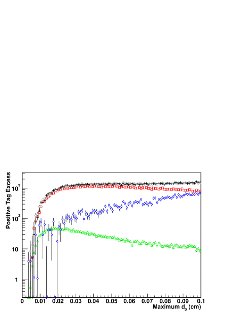
The set of jet probability tracks inside a tagged jet is used to build a variable sensitive to the flavor content of the jet itself. The relative contributions from heavy and light partons to data are determined by fitting the distribution of this variable for tagged jets in data to Monte Carlo simulation templates for , and light jets. For data, a sample selected by requiring a jet with 50 at the trigger level is used. For Monte Carlo simulation distributions, HERWIG is used to generate processes with an outgoing parton . We perform the fit using six different variables, the maximum impact parameter of the tracks in the jet, the maximum impact parameter significance of the tracks in the jet, the mass of the system of tracks with and , and the transverse momentum () with respect to the jet direction of the system of tracks with and .
The fit is made more robust by fitting the positive excess only, for which the distributions for negative tags are subtracted from the positive side. This removes contribution to the mistags due to detector resolution, which could be simulated poorly. The number of negative tags obtained for , and light jets in Monte Carlo simulation is normalized to the total number of negative tags found in data. From the fit, the fractions of , and light jets in data are obtained; thus the ratio of positive to negative tags from light jets, .
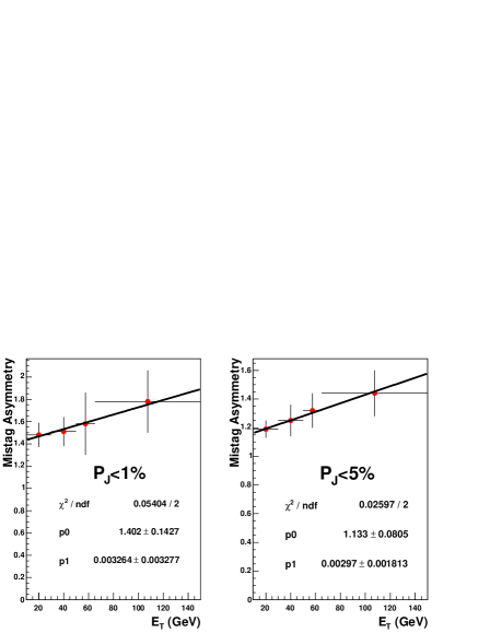
Figure 9 shows the result of the fit of the positive tag excess in data to Monte Carlo templates of the maximum impact parameter of the tracks contained within , and light tagged jets. A cut of 1% is used. It should be noted that the ratio gets a contribution from the tagging efficiency ratio of about 0.2. The observed rise of light jets is the result of the fact that tags for light jets are usually due to one large impact parameter track. Table 8 summarizes the results of the mistag asymmetry measurement with the six variables chosen for 1% and 5%. As a final estimate of the mistag asymmetry, we take the average of the six measurements and assign the maximum difference between the average and each single determination as the uncertainty. The results are and for cuts of 1% and 5%, respectively. The asymmetry is caused by secondary interactions with the detector material and residual lifetime effects from ’s and ’s, giving an excess of positive mistags. We study the expected contribution of ’s and ’s decays to the mistag asymmetry in Monte Carlo simulated events. We find the ratio of positively to negatively tagged light jets to be () for a cut of 1% (5%). Uncertainties are statistical only. These results are in good agreement with our measurements on data and suggest ’s and ’s to be the main source of mistag asymmetry. The negative tag rates measured have therefore to be scaled up by the asymmetry factor in order to obtain an accurate estimate of the positive mistag rate. We repeat the measurement in bins of jet transverse energy to study the dependence of the mistag asymmetry on the jet . Results are shown in Fig. 10. The asymmetry exhibits a small dependence with jet which is taken into account to estimate the mistag background.
| Fitted variable | ( 1%) | ( 5%) |
|---|---|---|
| Maximum | 1.64 0.02 | 1.37 0.02 |
| Maximum | 1.56 0.03 | 1.10 0.02 |
| Mass of the system of tracks with | 1.51 0.04 | 1.30 0.02 |
| Mass of the system of tracks with | 1.43 0.03 | 1.20 0.02 |
| P of the system of tracks with | 1.67 0.03 | 1.32 0.02 |
| of the system of tracks with | 1.57 0.02 | 1.30 0.02 |
| Average | 1.56 0.14 | 1.27 0.17 |
IV.3 Jet Probability Performance on Events
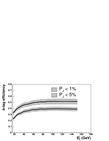
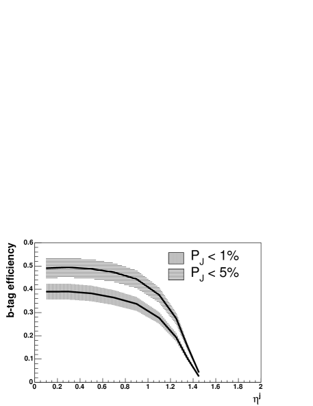
We study the performance of the jet probability algorithm by computing the efficiency to tag a jet in PYTHIA Monte Carlo events generated with a top mass = 178 . Results are shown in Fig. 11 as a function of the transverse energy and of the pseudo-rapidity of the jets for cuts of 1% and 5%. Jets are matched to quarks (by requiring between the reconstructed jet and the quark) and the tagging is applied to the resulting efficiency. We also measure the average efficiency to tag a or a jet in events passing the kinematic event selection described in Section V. Results are shown in Table 9 before and after applying the tagging . The scaled per-jet efficiencies, together with the mistag matrix, are used to determine the efficiency to tag at least jets per event, as described in Section VII. Although the tagging requirement results in some loss of efficiency for the signal, it significantly increases the signal-to-background ratio by heavily suppressing the dominant +jets background.
| b jets | c jets | |||
|---|---|---|---|---|
| Raw Eff. (%) | Scaled Eff. (%) | Raw Eff. (%) | Scaled Eff. (%) | |
| 1% | ||||
| 5% | ||||
V Event Selection
Top quark events in the lepton+jets channel are characterized by the presence of an electron or muon with high transverse energy, large missing transverse energy and four high energy jets, two of which are jets. The basic pretag selection requires one tight electron or muon, and jets with corrected and .
In order to select a lepton+jets sample completely disjoint from the top dilepton sample (), we reject events with an extra lepton that passes the loose requirements. Events consistent with are removed if a tight lepton and a second object form an invariant mass within the range [76, 106] . If the tight lepton is an electron, the second object may be an isolated electromagnetic object, a jet with electromagnetic fraction greater than 0.95 or an oppositely-signed isolated track. If the tight lepton is a muon, the second object may be an isolated muon or an opposite-signed isolated track.
The event vertex position is used to cluster jets and to ensure leptons and jets come from the same interaction. If more than one primary vertex is reconstructed in the event, the vertex closest to the lepton track is selected as event vertex. Events are rejected if the of the lepton track is farther than 5 cm from the of the event vertex. The vertex position is required to be within 60 cm of the center of the detector in order to ensure good event reconstruction in the projective tower geometry of the CDF detector. The efficiency of this requirement is measured using minimum bias data and found to be (95.1 0.3)%. For consistency with the -tagging algorithm, events are also rejected if the of the vertex with highest of all tracks is farther than 5 cm from the event vertex . The efficiency of this requirement is (98 2)%, where the 2% error accounts for the uncertainty in the simulation of multiple interactions.
The events selected by the above criteria are dominated by QCD production of bosons in association with jets. Figure 12 shows the distribution for taggable jets in this sample. In order to improve the signal to background ratio for events, we require at least one jet in the event to be tagged as a jet. A event is expected to have four jets in the final state, but due to gluon radiation, jet merging, and inefficiencies in jet reconstruction, this number can eventually be different. We therefore use the tagged events with three or more jets to define our signal sample, while the events with one and two jets are used as a control sample.

V.1 Optimized Selection
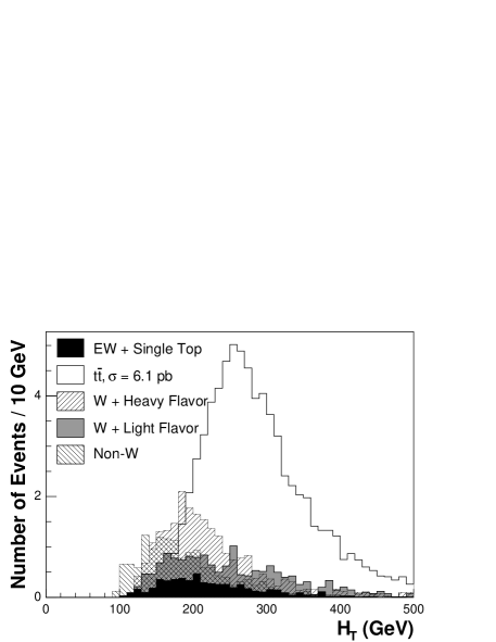
The variable , defined as the scalar sum of all the transverse energy in the event, i.e., the sum of the , the electron or muon , and the of the jets, is a measure of the energy in the hard scatter, and is a powerful discriminant between the pair production signal events () and background events (). In order to find the optimal cut, we maximize the statistical significance () in the signal region. Figure 13 (top) shows the distribution of the Monte Carlo simulation, together with the various background contributions, properly normalized. Figure 13 (bottom) shows the statistical significance as a function of the cut. Details about the background estimates and datasets used can be found in Section VI. Optimal statistical significance is reached with a cut of 200 .

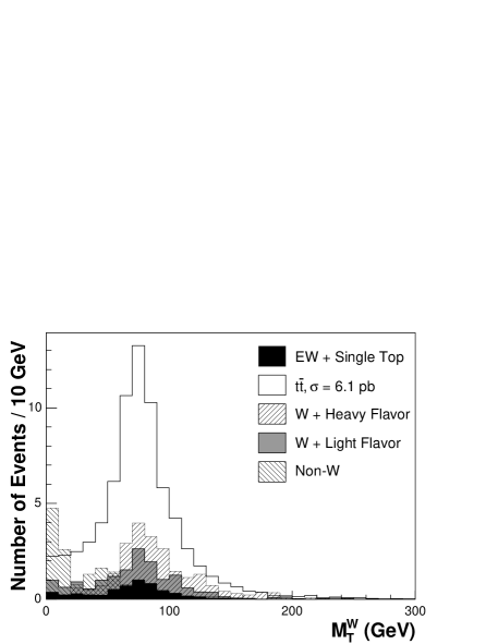
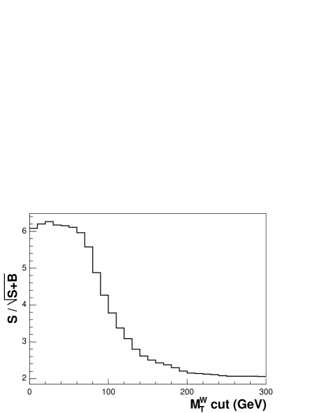
In addition, we enhance the component of the sample by requiring the transverse mass of the lepton and the missing energy, , be consistent with boson production. Figure 14 (top) shows the distribution for the Monte Carlo simulation together with the various normalized background contributions. Figure 14 (bottom) shows the statistical significance as a function of the cut. Note that the non- background lies at lower values of . In the optimization of the cut, we take to be the number of events from real bosons and to be the number of events from non-W background. A cut of gives optimal statistical significance.
V.2 Yields of Events
Events which pass the selection criteria described so far, before applying -tagging, form the pretag sample. The number of observed events in both the pretag and tagged samples for 1% and 5% are summarized in Table 10 as a function of the number of tight jets in the event.
| Jet Multiplicity | 1 jet | 2 jets | 3 jets | 4 jets |
|---|---|---|---|---|
| Pretag Events | ||||
| CEM | 16897 | 2657 | 182 | 105 |
| CMUP | 8169 | 1175 | 83 | 44 |
| CMX | 4273 | 610 | 35 | 17 |
| Total | 29339 | 4442 | 300 | 166 |
| Single Tagged Events, 1% (5%) | ||||
| CEM | 207 (571) | 106 (230) | 33 (53) | 36 (53) |
| CMUP | 92 (256) | 58 (105) | 13 (24) | 24 (29) |
| CMX | 51 (148) | 27 (50) | 6 (10) | 8 (11) |
| Total | 350 (975) | 191 (385) | 52 (87) | 68 (93) |
| Double Tagged Events, 1% (5%) | ||||
| CEM | — | 8 (16) | 7 (15) | 9 (18) |
| CMUP | — | 3 (9) | 4 (4) | 8 (17) |
| CMX | — | 2 (3) | 1 (3) | 1 (4) |
| Total | — | 13 (28) | 12 (22) | 18 (39) |
VI Backgrounds: Expected Composition of the -Tagged Lepton+Jets Sample
Other processes besides are expected to contribute to the tagged lepton+jets sample. The main contribution comes from heavy flavor production in association with a boson (, , ). +light flavor production also gives a significant contribution due to mistagged jets. Smaller contributions come from electroweak processes (diboson production, events or single top) and generic QCD jet production with misidentified bosons. These backgrounds are described in the following subsections.
VI.1 Electroweak Processes
Electroweak processes are studied using Monte Carlo simulated samples. Diboson events (, and ) can contribute to the tagged lepton+jets sample when one boson decays leptonically and the other decays into heavy quarks. The process can also give a contribution due to the leptonic decays of the tau. Finally, there is a contribution from single top quarks produced in association with a quark through annihilation in (s-channel) or -gluon fusion (t-channel), in which an initial gluon splits into a pair and a b quark interacts with a virtual W.
The number of events from these processes are predicted based on their theoretical cross sections bib:9 ; bib:9.5 ; bib:incW (listed in Table 11), the measured integrated luminosity, and the acceptances and tagging efficiencies derived from Monte Carlo simulations. The expectations for these backgrounds are corrected for differences between Monte Carlo simulations and data, which include the lepton identification scale factor, trigger efficiencies, the vertex cut efficiency and the tagging scale factor.
The total diboson, and single top predictions for 1% (5%) are shown in Table 19 (Table 20) and account for 2.5% (3.0%) of the number of events in the signal region of 3 and 4 jets. Following the same procedure, we also compute the electroweak background contributions to the pretag sample. The results are shown in Table 18.
| Process | Cross Section () |
|---|---|
| 13.25 0.25 | |
| 3.96 0.06 | |
| 1.58 0.02 | |
| Single Top (t-channel) | 1.98 0.08 |
| Single Top (s-channel) | 0.88 0.05 |
| 254.3 5.4 |
VI.2 Non-W Background
The non- background consists of events for which the lepton+ signature is not due to the decay of a boson. The main contribution to this source of background comes from QCD jet production where a jet provides the signature of a lepton and the missing transverse energy is due to a bad measurement of the jet energies. Semileptonic decays of mesons and misidentified photon conversions can also contribute. Due to its inherent instrumental nature, this background is difficult to estimate. In the event selection, its contribution to the lepton+jets sample is minimized by the requirement on the boson transverse mass . In particular, note that the optimization of this cut has been performed by requiring the lepton to be non-isolated in order to have an independent data sample to construct the kinematical variables (we use region C of Fig. 15).
The method used to estimate the non- background assumes that the isolation of the high- lepton and the event are uncorrelated for QCD processes, so that the ratio of non- events with low lepton isolation to those with high lepton isolation in the region at low is the same as in the high region. Four regions in the lepton isolation missing transverse energy plane are defined (see Fig. 15):
-
•
Region A: Isolation 0.2 and 15
-
•
Region B: Isolation 0.1 and 15
-
•
Region C: Isolation 0.2 and 20
-
•
Region D: Isolation 0.1 and 20 .
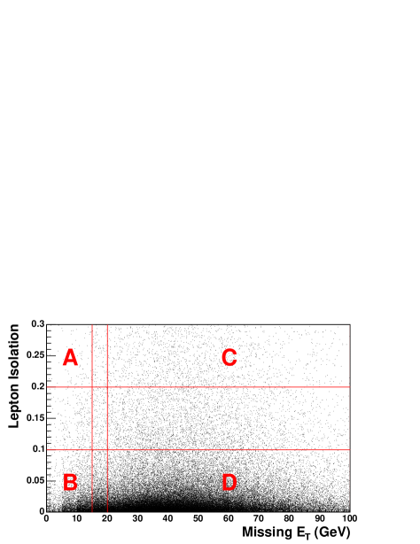
The signal is expected to populate region D (signal region), while the non- events dominate regions A, B and C (sideband regions). We can therefore estimate the fraction of events in the signal region which originate from non-W backgrounds as follows:
| (12) |
where , , and are the total numbers of observed events in the four regions. We describe next the estimate of the non- events in both the pretag and tagged samples.
VI.2.1 Fraction of non-W Events in the Pretag Sample
An estimate of the contribution of the non- events to the pretag sample is mandatory to correctly normalize most of the backgrounds in the tagged sample. Table 12 summarizes the results for the non- fractions in the pretag sample as a function of the jet multiplicity for electrons and muons. Note that we do not apply the and cuts in regions A and B to preserve statistics. We correct the yields in regions A, B and C by subtracting the expected contribution from events assuming (this assumption is found to have a negligible impact on the final non- estimate). Uncertainties in Table 12 are statistical only. The main source of systematic uncertainty comes from the lepton isolation and missing transverse energy not being fully uncorrelated for QCD events. We study the effect of this assumption by varying the values of the and lepton isolation cuts in the definition of the sideband regions. We observe a maximum variation of in the resulting non- fraction, which we assign as a systematic uncertainty on our estimates.
| Jet Multiplicity | 1 jet | 2 jets | 3 jets | 4 jets |
|---|---|---|---|---|
| Pretag Electrons | ||||
| Region A | 100600 | 12756 | 1745 | 216 |
| Region B | 61818 | 5228 | 593 | 98 |
| Region C | 1651 | 428 | 27 | 15 |
| Region D | 16897 | 2657 | 182 | 105 |
| F | 0.060 0.002 | 0.066 0.004 | 0.05 0.01 | 0.06 0.02 |
| Fnon-W | 0.060 0.002 | 0.066 0.004 | 0.05 0.01 | 0.05 0.02 |
| Pretag Muons | ||||
| Region A | 36599 | 5248 | 657 | 97 |
| Region B | 11718 | 968 | 114 | 21 |
| Region C | 737 | 181 | 12 | 11 |
| Region D | 12442 | 1785 | 118 | 61 |
| F | 0.0190 0.0007 | 0.019 0.002 | 0.018 0.006 | 0.04 0.02 |
| Fnon-W | 0.0190 0.0007 | 0.019 0.002 | 0.014 0.005 | 0.03 0.01 |
To further cross check the accuracy of the predictions, we define new intermediate isolation regions B′ and D′:
-
•
Region B: , Isol Region B′: , 0.1Isol,
-
•
Region D: , Isol Region D′: , 0.1Isol.
From the intermediate region B′, we estimate the number of non- events in region D′. The predicted non- fractions are shown in Table 13. The uncertainties quoted are statistical only. In the same table, these fractions are compared with the expected non- fractions computed from the difference between the observed events and the contributions from and jets events. The expected number of events is derived by normalizing the Monte Carlo prediction to a cross section of . In order to estimate the jets contribution in region D′, we compute the ratio of +jets events in the regions D′ and D using simulations and normalize the expectations for +jets production in D′ to the number of events in the signal region after removing , electroweak contributions. We compute the relative differences as the ratio of the difference between expected and predicted non- fractions to the predicted fraction. For each jet multiplicity bin, the differences between predicted and expected non- fractions in region D′ are consistent with the uncertainty we derived varying the and lepton isolation cuts in the definition of the sideband regions.
| Jet Multiplicity | 1 jet | 2 jets | 3 jets | 4 jets |
|---|---|---|---|---|
| Electron+Jets Sample | ||||
| Predicted Non- Fraction | 0.82 0.03 | 0.60 0.05 | 0.53 0.16 | 0.49 0.21 |
| Expected Non- Fraction | 0.78 0.01 | 0.82 0.02 | 0.76 0.10 | 0.59 0.16 |
| Fractional Relative Difference | -0.05 | 0.37 | 0.42 | 0.20 |
| Muon+Jets Sample | ||||
| Predicted Non- Fraction | 0.41 0.03 | 0.41 0.06 | 0.40 0.23 | 0.40 0.33 |
| Expected Non- Fraction | 0.70 0.02 | 0.62 0.05 | 0.44 0.22 | 0.26 0.25 |
| Fractional Relative Difference | 0.70 | 0.50 | 0.11 | -0.35 |
VI.2.2 Non-W Events in the Tagged Sample
The non- background contributes to the tagged sample through both real heavy flavor production ( and events) and mistags. We compute the number of non- events with tagged jets in the signal region using equation 12 with the numbers of tagged events in the sideband regions. Yields in regions A, B and C are corrected for contributions. The results are summarized in Table 14: is the ratio of tagged events in regions B and A and it is used to normalize the number of tagged events in the region C to get the expected number of non-W events on the signal region. The precision of these estimates is limited by the number of tagged events in the sideband regions.
| Jet Multiplicity | 1 jet | 2 jets | 3 jets | 4 jets |
|---|---|---|---|---|
| Electron+Jets Sample ( 1%) | ||||
| 0.36 0.01 | 0.26 0.02 | 0.26 0.05 | 0.4 0.2 | |
| 74.8 | 25.1 | 1.8 | 1.0 | |
| 26.7 3.3 | 6.6 1.4 | 0.5 0.4 | 0.4 0.4 | |
| Muon+Jets Sample ( 1%) | ||||
| 0.102 0.008 | 0.10 0.02 | 0.11 0.04 | 0.2 0.1 | |
| 36.9 | 20.3 | 4.0 | 0.81 | |
| 3.8 0.7 | 2.0 0.6 | 0.5 0.3 | 0.2 0.1 | |
| Electron+Jets Sample ( 5%) | ||||
| 0.42 0.01 | 0.33 0.02 | 0.29 0.04 | 0.5 0.1 | |
| 142.8 | 52.9 | 3.5 | 1.5 | |
| 59.6 5.2 | 17.6 2.6 | 1.0 0.5 | 0.7 0.6 | |
| Muon+Jets Sample ( 5%) | ||||
| 0.141 0.007 | 0.12 0.01 | 0.09 0.03 | 0.17 0.07 | |
| 65.8 | 32.1 | 3.7 | 0.6 | |
| 9.3 1.2 | 3.8 0.8 | 0.3 0.2 | 0.1 0.1 | |
We cross check these results by estimating the non- contribution to the tagged lepton+jets sample following two alternative methods. In the first one (), we assume the tag rate in region D to be the same as in region B:
| (13) |
where is the event tag rate in region B and is the number of events in region D. This method has a large systematic uncertainty since the tag rate could depend on the missing transverse energy due to the contribution of events with a quark decaying into leptons. Events with large would have a larger heavy flavor contribution due to real neutrino production from semileptonic decay. In the second alternative method (), we compute the tagging rates per jet in the sideband regions, and then we predict the tag rate per jet in the signal region D as
| (14) |
We compute the jet tagging rate by assuming it to be the same in all the jet multiplicity bins and use this estimate to predict the non- background in the signal region taking into account the jet multiplicity and the number of non- events expected in the pretag lepton+jets sample. Table 15 compares the non- contributions predicted by the three methods.
| Jet Multiplicity | 1 jet | 2 jets | 3 jets | 4 jets |
|---|---|---|---|---|
| 1% | ||||
| 30.5 3.3 | 8.6 1.5 | 0.9 0.5 | 0.5 0.4 | |
| 19.0 0.7 | 6.7 0.6 | 0.6 0.1 | 0.6 0.3 | |
| 27.7 2.6 | 9.3 0.9 | 0.7 0.1 | 0.6 0.2 | |
| 5% | ||||
| 68.8 5.4 | 21.4 2.8 | 1.3 0.6 | 0.8 0.6 | |
| 43.5 1.3 | 16.2 1.0 | 1.1 0.2 | 1.6 0.5 | |
| 65.4 4.4 | 21.9 1.8 | 1.6 0.3 | 1.5 0.4 | |
Finally, we use the results of the two alternative estimates to assign a systematic uncertainty of 50% which takes into account the differences with the base method. The total non- background accounts for 1.2% of the observed events with tagged jets in the signal region, both for 1% and 5%.
VI.3 W + Heavy Flavor Processes
+heavy flavor production is the main source of background in the tagged lepton+jets sample. It is estimated using the heavy flavor fractions in boson production in association with partons and the tagging efficiency for these processes. These quantities are derived from Monte Carlo simulations. The overall normalization is obtained from the number of observed events in the pretag sample.
The estimate of the heavy flavor fraction in +jets events is described elsewhere bib:secvtx . We use the ALPGEN event generator, which is able to compute exact matrix element calculations at leading order for parton level QCD and electroweak processes. We can therefore compute the ratio between the +heavy flavor production cross section and the inclusive +jets cross section since it is expected to be stable in the transition from leading-order to next-to-leading-order matrix elements. We generate events where inclusive , , and are produced in association with light partons. Parton level events from ALPGEN are fed to the HERWIG parton shower program which generates additional jets from gluon radiation, and a full CDF detector simulation is applied. Events containing a different number of light partons are combined following a rigorous prescription in order to avoid double counting due to parton shower radiation, which causes parton events to populate part of the phase space described by the () parton sample. The and samples are further divided into two classes according to the number of reconstructed heavy flavor jets in the event. We refer to these classes as 1B and 2B (1C and 2C) for (). By means of these combined Monte Carlo simulated samples, the heavy flavor fractions for +jets events are measured as the ratio between the computed +heavy flavor and +jets cross sections. Jet data samples are used to correct for residual discrepancies between data and Monte Carlo simulations: a factor 1.5 0.4 is applied to the and fractions bib:secvtx , where the uncertainty is dominated by the systematic uncertainties associated with the ALPGEN heavy flavor calculations. The final heavy flavor fractions are shown in Table 16.
| Jet Multiplicity | 1 jet | 2 jets | 3 jets | 4 jets |
|---|---|---|---|---|
| 1B | 0.010 0.003 | 0.014 0.004 | 0.024 0.006 | 0.022 0.006 |
| 2B | — | 0.014 0.004 | 0.023 0.006 | 0.026 0.007 |
| 1C | 0.016 0.004 | 0.024 0.006 | 0.038 0.010 | 0.035 0.010 |
| 2C | — | 0.018 0.005 | 0.029 0.008 | 0.037 0.010 |
| 0.043 0.009 | 0.060 0.013 | 0.060 0.013 | 0.059 0.013 |
| Jet Multiplicity | 1 jet | 2 jet | 3 jet | 4 jets |
|---|---|---|---|---|
| Event Tagging Efficiencies (%), 1% | ||||
| 1B (1 tag) | 29.5 0.3 2.5 | 30.7 0.6 2.6 | 37.0 1.5 3.2 | 33.5 3.2 2.9 |
| 2B (1 tag) | — | 50.5 0.7 4.3 | 56.0 1.6 4.8 | 54.6 2.2 4.7 |
| 1C (1 tag) | 6.8 0.2 0.9 | 7.8 0.4 1.0 | 9.1 1.0 1.2 | 8.0 1.9 1.0 |
| 2C (1 tag) | — | 13.5 0.6 1.7 | 16.8 1.5 2.2 | 14.3 1.7 1.8 |
| Wc (1 tag) | 7.2 0.2 0.9 | 7.9 0.3 1.0 | 8.3 0.9 1.1 | 6.9 1.1 0.9 |
| Event Tagging Efficiencies (%), 5% | ||||
| 1B (1 tag) | 39.6 0.3 3.4 | 40.8 0.6 3.4 | 47.1 1.6 4.0 | 41.4 3.4 3.5 |
| 2B (1 tag) | — | 63.5 0.7 5.4 | 68.4 1.5 5.8 | 66.7 2.1 5.6 |
| 1C (1 tag) | 14.8 0.3 1.9 | 17.2 0.5 2.2 | 18.7 1.4 2.4 | 16.3 2.6 2.1 |
| 2C (1 tag) | — | 27.1 0.8 3.4 | 33.2 1.9 4.2 | 32.3 2.3 4.1 |
| Wc (1 tag) | 15.3 0.3 1.9 | 16.4 0.5 2.1 | 19.4 1.3 2.5 | 18.6 1.7 2.4 |
The contribution of +heavy flavor production to the pretag lepton+jets sample is estimated by multiplying heavy flavor fractions by the observed number of events in the pretag sample, corrected for the non-, and electroweak background expectations. The results are shown in Table 18.
The above Monte Carlo simulated samples after pretag selection are used to compute the tagging efficiencies. In order to avoid double counting of the mistag background, the jet probability algorithm is applied only to jets known to be due to a or quark. Each tagged jet is weighted according to the scale factor. Results are summarized in Table 17. The systematic uncertainties are dominated by the uncertainties on the scale factor for and jets. The pretag expectations are multiplied by the tagging efficiencies to estimate the contributions of these processes to the tagged sample. The numbers of , and events expected in the tagged lepton+jets sample for 1% (5%) are shown, along with the rest of the backgrounds, in Table 19 (Table 20) and account for 12.3% (13.2%) of the observed number of events in the signal region.
VI.4 Mistag Background
Events in which jets from light partons are tagged as heavy flavor jets can contribute to the tagged sample. The number of events with negative tags in the pretag sample would be a simple estimate of this background, but this method has the problem of a large statistical uncertainty. Instead, we count the events in the pretag sample weighted by their probability to have at least one mistagged jet. This probability is computed by applying the negative tag rate matrix to all the taggable jets in the event.
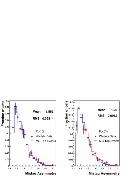
This estimate is corrected for the mistag asymmetry derived in Section IV.2.1. In order to take into account the dependence of the mistag asymmetry on the jet , we convolute it with the jet spectra in events with +three or more jets for data and Monte Carlo simulation, as shown in Fig. 16. The observed difference between the means of the distributions and the mistag asymmetry values measured in Section IV.2.1 are negligible within the uncertainties. We therefore decide to use the former in our analysis. The RMS of the distributions gives an estimate of how much the asymmetry changes over the jets in our samples, and it is taken as an additional uncertainty on the mistag asymmetry. The final mistag asymmetry scale factors are 1.56 0.17 for 1% and 1.27 0.20 for 5%.
The estimate of the mistag background is also scaled down by one minus the fraction of pretag events which are due to non-, and electroweak backgrounds. The contribution of the mistag background to the lepton+jets sample when a jet with 1% (5%) is required is shown in Table 19 (Table 20) and accounts for 12.8% (27.9%) of the observed number of events in the signal region.
VI.4.1 Mistag Cross Check
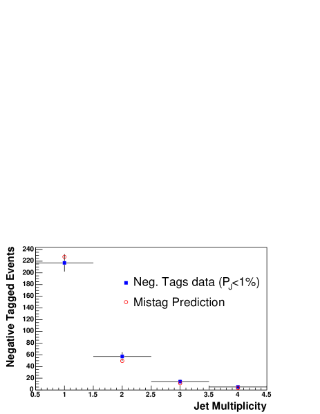
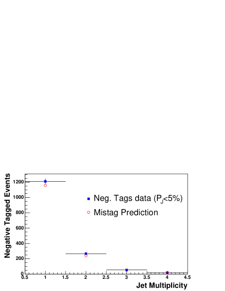
The negative tag rate matrix has been extensively tested on inclusive jet samples. Results are discussed in Section IV.2. The mistag matrix is found to correctly predict the number of events with negatively tagged jets observed in independent samples to within a few percent. To further test the mistag matrix reliability on lepton+jets data, we select a subsample of events by requiring . This sample is expected to be dominated by QCD jet production with the high- lepton signature provided by a jet. Figure 17 compares the observed number of events with negative tags and the matrix prediction as a function of the jet multiplicity. Good agreement is observed confirming the reliability of the mistag matrix to predict the negative tag rate in events dominated by prompt jets.
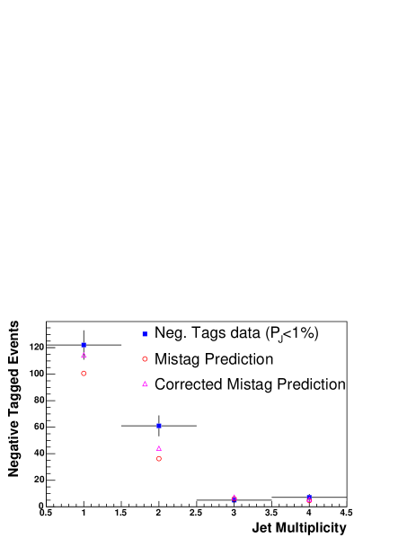
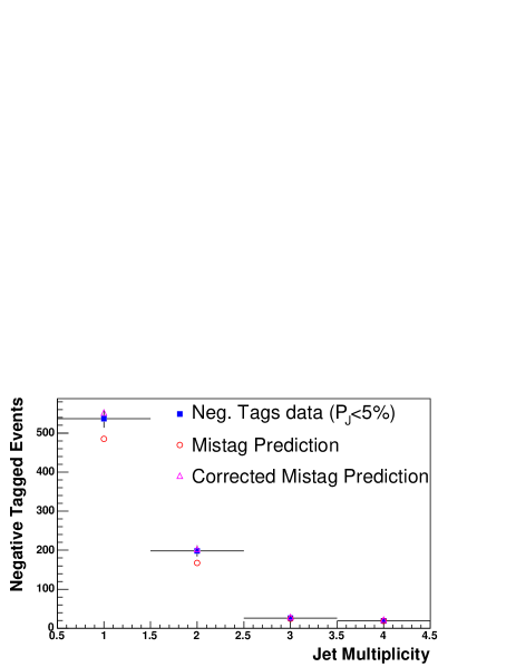
We repeat the test on the pretag lepton+jets sample, where a requirement is applied. Results are shown in Fig. 18. We observe a discrepancy between observed and predicted negative tags which we attribute to the higher fraction of heavy flavor in lepton+jets events with high value of with respect to the inclusive jet samples where the matrix has been computed. To corroborate this hypothesis, we make a first-order correction to the mistag prediction by using the heavy flavor fractions () in +jets events (see Table 16). We compute the negative tag rates for light () and heavy () flavor jets in Monte Carlo simulation. For each jet multiplicity bin, a scale factor is then determined as:
| (15) | |||||
| (16) |
where
| (17) |
The numbers and in the formula are the jet multiplicity and the number of heavy flavor jets ( for , or and for or ), respectively. The corrected distributions, also shown in Fig. 18, show a much better agreement with the observed rates of negative tagged events.
We therefore use the mistag matrix prediction corrected by the mistag asymmetry as an estimate of the number of events with a tagged light jet.
VI.5 Background Summary
Table 18 summarizes the contributions of the different background estimates in the pretag sample. The difference between the observed number of events and the total background estimate is due to +light flavor and contributions.
| Jet Multiplicity | 1 jet | 2 jets | 3 jets | 4 jets |
|---|---|---|---|---|
| Electroweak | ||||
| 127 9 | 123 9 | 10.0 0.8 | 3.6 0.3 | |
| 16.8 1.2 | 18.8 1.4 | 1.7 0.1 | 0.61 0.06 | |
| 0.67 0.05 | 0.68 0.05 | 0.14 0.02 | 0.052 0.008 | |
| Single Top | 13.4 1.1 | 13.6 1.1 | 1.44 0.12 | 0.38 0.04 |
| Single Top | 4.0 0.4 | 7.9 0.7 | 1.02 0.10 | 0.24 0.02 |
| 87 7 | 16.5 1.7 | 1.0 0.3 | 0 0 | |
| Total | 249 18 | 180 13 | 15.3 1.2 | 4.9 0.4 |
| W + Heavy Flavor | ||||
| 281 75 | 116 31 | 12.9 3.3 | 7.4 2.0 | |
| 459 123 | 170 46 | 18.4 5.0 | 11.1 3.1 | |
| 1197 252 | 243 53 | 16.9 3.6 | 9.1 2.0 | |
| Total | 1938 322 | 530 94 | 47.8 9.0 | 27.5 5.5 |
| Others | ||||
| Non- | 1250 626 | 208 104 | 10.0 5.3 | 7.3 4.1 |
| Total Background | 3436 741 | 917 150 | 73 11 | 39.7 7.2 |
| Data | 29339 | 4442 | 300 | 166 |
Table 19 and Table 20 summarize the contributions of the different background sources in the tagged lepton+jets sample for 1% and 5% respectively.
| Jet Multiplicity | 1 jet | 2 jets | 3 jets | 4 jets |
|---|---|---|---|---|
| Electroweak | ||||
| 2.2 0.3 | 5.0 0.6 | 0.7 0.1 | 0.28 0.06 | |
| 1.0 0.1 | 2.0 0.2 | 0.23 0.03 | 0.09 0.02 | |
| 0.027 0.006 | 0.09 0.01 | 0.012 0.004 | 0.007 0.002 | |
| Single Top | 4.1 0.5 | 4.9 0.6 | 0.73 0.08 | 0.20 0.02 |
| Single Top | 1.3 0.2 | 4.2 0.5 | 0.60 0.07 | 0.14 0.02 |
| 0.7 0.3 | 0.4 0.2 | 0.04 0.04 | 0 0 | |
| Total | 9.3 1.1 | 16.6 1.8 | 2.3 0.3 | 0.71 0.09 |
| W + Heavy Flavor | ||||
| 83 23 | 47 13 | 6.0 1.6 | 3.3 0.9 | |
| 31 9 | 17.5 5.2 | 2.3 0.7 | 1.2 0.4 | |
| 86 21 | 19.2 5.0 | 1.4 0.4 | 0.6 0.2 | |
| Total | 200 42 | 84 20 | 9.6 2.4 | 5.2 1.4 |
| Others | ||||
| Mistag | 149 17 | 51.8 5.9 | 8.5 1.0 | 6.7 0.8 |
| Non- | 31 16 | 8.6 4.6 | 0.9 0.6 | 0.5 0.5 |
| Total Background | 389 49 | 161 22 | 21.4 2.7 | 13.1 1.7 |
| Data | 350 | 191 | 52 | 68 |
| Jet Multiplicity | 1 jet | 2 jets | 3 jets | 4 jets |
|---|---|---|---|---|
| Electroweak | ||||
| 5.5 0.6 | 12.5 1.4 | 1.81 0.21 | 0.74 0.10 | |
| 1.6 0.2 | 3.3 0.3 | 0.40 0.05 | 0.16 0.02 | |
| 0.049 0.009 | 0.14 0.02 | 0.027 0.006 | 0.014 0.004 | |
| Single Top | 5.4 0.6 | 6.5 0.7 | 0.92 0.10 | 0.26 0.03 |
| Single Top | 1.7 0.2 | 5.2 0.6 | 0.74 0.08 | 0.17 0.02 |
| 2.1 0.5 | 1.1 0.3 | 0.13 0.10 | 0 0 | |
| Total | 16.3 1.8 | 28.8 3.0 | 4.0 0.4 | 1.4 0.1 |
| W + Heavy Flavor | ||||
| 111 31 | 61 17 | 7.4 2.0 | 4.1 1.2 | |
| 68 20 | 36 11 | 4.6 1.4 | 2.7 0.8 | |
| 184 45 | 40 10 | 3.2 0.8 | 1.7 0.5 | |
| Total | 363 75 | 137 31 | 15.2 3.6 | 8.5 2.1 |
| Others | ||||
| Mistag | 585 92 | 194 30 | 28.2 4.4 | 22.1 3.5 |
| Non- | 69 35 | 21 11 | 1.3 0.9 | 0.79 0.74 |
| Total Background | 1033 125 | 381 46 | 48.8 5.9 | 32.7 4.2 |
| Data | 975 | 385 | 87 | 93 |
We observe good agreement between data and background predictions in events with one and two jets, which supports the validity of our background estimates. In events with three or more jets, we observe an excess of tagged events in data which we attribute to events. The estimates of the +heavy flavor and mistag background contributions have been normalized to the data in the pretag sample assuming no signal. Having actually observed a significant number of events in the tagged sample, we need to correct those estimates by the number of signal events in the pretag sample. We make this correction through an iterative procedure which is described in Section VIII.
VII Signal Acceptance
The signal acceptance, or event detection efficiency, is defined as the fraction of events that satisfy all selection requirements, and includes trigger and reconstruction efficiencies as well as the efficiencies of the kinematic selection and of the -tagging algorithm. We measure it using a PYTHIA Monte Carlo sample generated with a top quark mass and simulated as discussed in Section III. Wherever possible, effects which are not sufficiently well modeled in the simulation are measured using data. The acceptance is defined as
| (18) |
where is the fraction of Monte Carlo simulated events which pass the kinematic requirements (except -tagging) and includes the branching fraction for , the lepton identification efficiency (including isolation and cosmic/conversion veto efficiency, as described in Section III), the dilepton and veto efficiencies, and the kinematic and geometric acceptances. is measured separately for electron and muon events. is a scale factor which takes into account the difference in lepton identification efficiency between data and Monte Carlo simulations estimated using events; is the trigger efficiency for identifying high leptons and is measured using data from independent triggers. Both and are discussed in Section III. and are the efficiencies for the vertex cuts described in Section V and is the efficiency to tag at least one tight jet in a event and includes a tagging scale factor to account for differences between Monte Carlo simulations and data.
| Quantity | CEM | CMUP | CMX |
|---|---|---|---|
| 3.67 0.02 0.22 | 1.92 0.01 0.12 | 0.751 0.008 0.046 | |
| () | 318 19 | 318 19 | 305 18 |
| Single Tag, 1%, = 0.817 0.070 | |||
| 54.7 0.2 3.6 | 54.1 0.3 3.5 | 55.2 0.5 3.6 | |
| Average | 54.5 0.2 3.6 | ||
| 2.00 0.01 0.18 | 1.04 0.01 0.09 | 0.41 0.01 0.04 | |
| () | 6.38 0.04 0.68 | 3.30 0.03 0.36 | 1.32 0.02 0.14 |
| Total | pb-1 | ||
| Single Tag, 5%, = 0.852 0.072 | |||
| 68.8 0.2 3.7 | 68.6 0.3 3.7 | 69.6 0.5 3.7 | |
| Average | 68.8 0.2 3.7 | ||
| 2.52 0.01 0.20 | 1.315 0.009 0.108 | 0.523 0.006 0.042 | |
| () | 8.03 0.05 0.80 | 4.19 0.03 0.42 | 1.67 0.02 0.17 |
| Total | pb-1 | ||
The event tagging efficiency is obtained from the same Monte Carlo simulated sample. We compute, for each event, the probability of having tagged jets in the event by assigning to each jet a probability to be tagged. The sum of these probabilities over all the events returns the number of expected events with at least tags, from which we calculate the tagging efficiency. For light flavor jets, this probability is computed using the mistag matrix, while for heavy flavor jets the probability is the value of the tagging scale factor (see Section IV) if the jet is tagged and zero otherwise. We estimate the systematic uncertainty on the event tagging efficiency by varying the tagging scale factor and mistag prediction by .
Table 21 summarizes the acceptance for events. For cuts of 1% and 5%, the combined acceptance times integrated luminosity are, respectively, pb-1 and pb-1, where the statistical uncertainty is uncorrelated between the lepton types, and the systematic uncertainty is assumed to be 100% correlated since it is dominated by the luminosity and tagging scale factor uncertainties.
Table 22 summarizes the contributions to the systematic uncertainty on the signal acceptance. Trigger, lepton identification and vertex cuts have already been discussed in Sections III and V. The observed difference in the conversion veto efficiency between events and the sample used to measure the electron identification scale factor is added as an uncertainty on the tight electron identification efficiency. The efficiency of the cosmic ray veto is measured from data and accounts for a 1% uncertainty on the tight muon identification efficiency. Additional uncertainties in the electron (muon) acceptance are due to () scale, () resolution and material (geometrical) effects, and are found to be 0.3% (1.2%) in inclusive events. The lepton isolation uncertainty accounts for differences in the modeling of the lepton identification in events with different jet multiplicity. It has been evaluated by comparing data to Monte Carlo simulations for +jets and events. The uncertainty due to the jet energy scale is estimated by the shift in signal acceptance observed by changing the jet energy corrections within their uncertainties. The uncertainty due to parton distribution functions (PDF) is estimated by re-weighting the events generated with CTEQ5L for different sets of PDFs bib:cteq5l . In particular, we consider the difference in signal acceptance between NLO CTEQ6M and CTEQ5L, between MRST for two different values of , and between NLO CTEQ6M and the 20 CTEQ eigenvectors, and we add in quadrature all the contributions. Differences in the modeling of production and decay are evaluated as the difference in acceptance between samples of signal events generated with HERWIG and PYTHIA. Samples of events with different levels of initial and final state radiation (ISR/FSR) are used to evaluate the effect of this source of uncertainty on the signal acceptance. The systematic uncertainty on the event tagging efficiency is estimated by varying the tagging scale factor and the mistag prediction by 1. The total systematic uncertainty on the signal acceptance is 8.9% (8.0%) for 1% (5%), and is dominated by the tagging scale factor and the jet energy scale uncertainties.
| Source | Relative Uncertainty (%) | Uncertainty on the Acceptance (%) |
| Central Electron Trigger | 0.6 | 0.3 |
| Central Electron ID | 0.5 | 0.3 |
| Conversion Veto Eff. | 1.4 | 0.8 |
| Scale of Electron | 0.3 | 0.2 |
| Central Muon Trigger | 0.5 | 0.2 |
| Central Muon ID | 1.0 | 0.3 |
| CMX Muon Trigger | 0.4 | 0.05 |
| CMX Muon ID | 0.6 | 0.07 |
| Cosmic Veto Eff. | 1.0 | 0.4 |
| Scale of Muon | 1.2 | 0.5 |
| Lepton Isolation | 2.0 | 2.0 |
| Cut Eff. | 0.3 | 0.3 |
| Cut Eff. | 2 | 2 |
| Jet Energy Scale | — | 4.2 |
| — | 2 | |
| MC Modeling | — | 1.6 |
| ISR/FSR | — | 1.3 |
| Tagging 1% (b’s/c’s) | 8.6/12.9 | 6.5 |
| Mistag Asymmetry 1% | 11.0 | 0.2 |
| Tagging 5% (b’s/c’s) | 8.5/12.7 | 5.4 |
| Mistag Asymmetry 5% | 15.5 | 0.4 |
| Total Uncertainty ( 1%) | — | 8.9 |
| Total Uncertainty ( 5%) | — | 8.0 |
VIII Cross Section for Single Tagged Events
We measure the cross section as
| (19) |
where is the observed number of events with at least one jet tagged, is the background estimate in the signal region, is the signal acceptance including the tagging efficiency and is the integrated luminosity. The estimated number of background events must be corrected for the contribution, since we normalize mistag and +heavy flavor backgrounds assuming no signal events in the pretag sample. We apply an iterative procedure in which we first estimate the number of tagged top candidates in the sample as the number of tagged signal events minus the total background in the 3 jet bins. Successively, the obtained signal cross section is used to estimate the number of events before the -tagging requirement, and this contribution is subtracted from the total number of events to which we normalize the mistag, , and backgrounds. The expectations for single top, diboson and Z do not change with the number of events in the signal region. The change for non- background is found to be negligible compared to its uncertainty. Therefore, this background is also kept fixed. Having obtained a new estimate for the tagged background, we re-evaluate the number of candidates. The procedure is repeated until the cross section changes by less than 0.1%.
Starting with the backgrounds shown in Tables 19 and 20, we apply the iterative procedure and measure
for 1%. As a cross check, we apply the iterative procedure for 5% and measure
The final signal and background estimates are shown in Table 23, together with the observed number of events.
| Jet Multiplicity | 1 jet | 2 jets | 3 jets | 4 jets |
|---|---|---|---|---|
| Pretag Data | 29339 | 4442 | 300 | 166 |
| 1% | ||||
| Electroweak | 9.3 1.1 | 16.6 1.8 | 2.3 0.3 | 0.71 0.09 |
| 83 23 | 47 13 | 4.3 1.2 | 1.1 0.3 | |
| 31 9 | 17.3 5.2 | 1.6 0.5 | 0.4 0.1 | |
| 86 21 | 19.0 4.9 | 1.0 0.3 | 0.21 0.06 | |
| Mistag | 149 17 | 51 6 | 6.1 0.7 | 2.2 0.3 |
| Non- | 31 16 | 8.6 4.6 | 0.9 0.6 | 0.5 0.5 |
| Total Background | 389 49 | 159 22 | 16.3 2.0 | 5.1 0.7 |
| (8.9 pb) | 2.5 0.5 | 20.6 2.4 | 40.4 4.5 | 58.1 6.2 |
| Data | 350 | 191 | 52 | 68 |
| 5% | ||||
| Electroweak | 16.3 1.8 | 28.8 3.0 | 4.0 0.4 | 1.4 0.1 |
| 111 31 | 60 17 | 5.2 1.4 | 1.1 0.3 | |
| 68 20 | 36 11 | 3.2 1.0 | 0.76 0.24 | |
| 184 45 | 40 10 | 2.2 0.6 | 0.5 0.13 | |
| Mistag | 585 92 | 191 30 | 19.6 3.1 | 6.1 1.0 |
| Non- | 69 35 | 21 11 | 1.3 0.9 | 0.8 0.7 |
| Total Background | 1033 125 | 377 46 | 35.5 4.2 | 10.6 1.4 |
| (9.6 pb) | 3.6 0.6 | 28.4 3.1 | 55.1 5.7 | 78.6 7.8 |
| Data | 975 | 385 | 87 | 93 |
Figure 19 compares the numbers of observed data to background and signal expectations, for 1% and 5%, for the measured production cross sections.
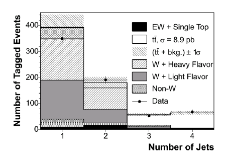
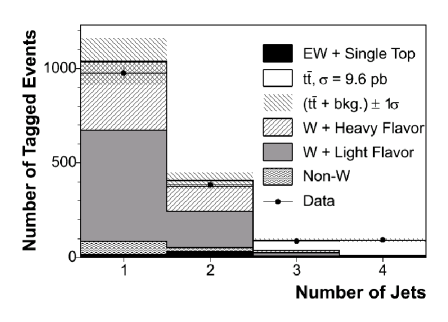
The statistical uncertainty on the measured cross section is dominated by the data sample size. Table 24 summarizes the systematic contributions to the cross section uncertainty. The correlations in acceptances, tagging scale factor and luminosity uncertainty are taken into account. and systematics are considered correlated across all the bins. All the other uncertainties are treated as uncorrelated.
| Source | Fractional Syst. Uncert. (%) | Contribution to (%) | |
|---|---|---|---|
| 1% | 5% | ||
| Central Electron ID | 1.6 | +0.99/-0.97 | +1.00/-0.98 |
| Central Muon ID | 1.9 | +0.61/-0.61 | +0.62/-0.61 |
| CMX Muon ID | 1.8 | +0.22/-0.22 | +0.22/-0.22 |
| 2 | +2.1/-2.0 | +2.1/-2.0 | |
| Jet Energy Scale | 4.2 | +4.5/-4.2 | +4.6/-4.2 |
| Lepton Isolation | 2 | +2.1/-2.0 | +2.1/-2.0 |
| ISR/FSR | 1.3 | +1.4/-1.3 | +1.4/-1.3 |
| MC Modeling | 1.6 | +1.7/-1.6 | +1.7/-1.6 |
| Z Vertex | 2.0 | +2.1/-2.1 | +2.2/-2.1 |
| Tagging 1% (b’s/c’s) | 8.6/12.9 | +8.2/-7.2 | — |
| Tagging 5% (b’s/c’s) | 8.5/12.7 | — | +7.0/-6.3 |
| Mistag Asymmetry 1% | 11.0 | +0.93/-0.93 | — |
| Mistag Asymmetry 5% | 15.5 | — | +3.0/-3.0 |
| Non- Fraction | 50 | 0.33 | 0.56 |
| Non- Prediction | 50 | 0.71 | 0.79 |
| +HF Prediction | 30 | 2.6 | 2.9 |
| Cross Sections Bck. | 1.8 | 0.056 | 0.072 |
| Luminosity | 5.9 | +6.5-5.7 | +6.5-5.8 |
| Total Systematic Uncertainty | +12.5/-11.3 | +12.3/-11.3 | |
VIII.1 Cross Section Dependence on the Top Quark Mass
The signal acceptance used in this analysis has been computed using a sample of events generated with PYTHIA for , which corresponds to the combined Run I top mass measurement at the Tevatron Collider bib:runimass . We study the dependence of the cross section on the top quark mass by reevaluating the signal acceptance through a set of Monte Carlo simulated samples generated by HERWIG for different values of the top mass. Results are shown in Fig. 20. A linear fit to the measured cross sections as a function of the top mass returns a slope of -0.052 0.008 pb/() and -0.066 0.008 pb/() for 1% and 5% respectively, where the uncertainties are due to Monte Carlo simulation statistics. Note that the fit results for agree with the measured cross section within the 1.6% uncertainty estimated in Section VII due to different modeling in PYTHIA and HERWIG.
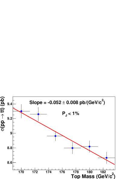
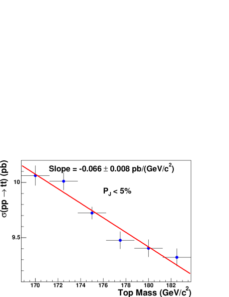
VIII.2 Electron versus Muon Cross Section Measurements
As an additional cross check, we measure the cross section separately for events with tight electrons and muons. Table 25 summarizes the cross sections for the two analyses with 1% and 5%. The cross section measurements in the electron and muon+jets samples agree within their statistical uncertainty.
| Total | Electrons | Muons | |
|---|---|---|---|
| 1% | 8.9(stat.)(syst.) | 8.6(stat.)(syst.) | 9.4(stat.)(syst.) |
| 5% | 9.6(stat.)(syst.) | 9.4(stat.)(syst.) | 9.9(stat.)(syst.) |
IX Cross Section for Double Tagged Events
The measurement of the ttbar cross section in a sample with at least two b tags follows the same procedure as the single tag analysis, with a much purer sample of events. As shown in Table 10, after requiring the event selection described in Section V, we observe 30 (61) events with two -tagged jets out of the 120 (180) events with at least one -tagged jet for 1% ( 5%). Table 26 shows the signal acceptances and the efficiencies to tag two jets in signal events passing the pretag selection. The total acceptance times luminosity for 1% and 5% is pb-1 and pb-1 respectively.
| Quantity | CEM | CMUP | CMX |
|---|---|---|---|
| 3.67 0.02 0.22 | 1.92 0.01 0.12 | 0.751 0.008 0.046 | |
| () | 318 19 | 318 19 | 305 18 |
| Double Tag, 1%, = 0.817 0.070 | |||
| 12.7 0.2 2.1 | 12.6 0.2 2.0 | 13.4 0.4 2.2 | |
| Average | 12.7 0.1 2.1 | ||
| 0.465 0.006 0.081 | 0.241 0.004 0.042 | 0.101 0.003 0.018 | |
| () | 1.48 0.02 0.27 | 0.77 0.01 0.14 | 0.32 0.01 0.06 |
| Total | pb-1 | ||
| Double Tag, 5%, = 0.852 0.072 | |||
| 24.4 0.2 3.6 | 24.1 0.3 3.6 | 25.2 0.5 3.7 | |
| Average | 24.4 0.2 3.6 | ||
| 0.895 0.009 0.142 | 0.462 0.006 0.074 | 0.189 0.004 0.030 | |
| () | 2.85 0.03 0.48 | 1.47 0.02 0.25 | 0.60 0.01 0.10 |
| Total | pb-1 | ||
IX.1 Backgrounds in the Double -Tag Sample
A few differences with respect to the single tag analysis must be taken into account in order to estimate the backgrounds. We define the mistag background as the events with at least two mistagged jets. The negative tag rate matrix is applied to negatively taggable jets in the event and the probability to have at least two mistagged jets is summed over all events. The mistag prediction is scaled by the fraction of non-, electroweak backgrounds and by the mistag asymmetry as is done for the single tag analysis.
Events with one real heavy flavor tag plus a mistag are included in the other background sources. The contribution of mistags to the +heavy flavor background is taken into account by applying the mistag rate matrix to light flavor jets in events with an extra real tag when computing the tagging efficiency. Results are summarized in Table 27.
| jet multiplicity | 2 jets | 3 jets | 4 jets |
|---|---|---|---|
| Double Tag Tagging Efficiencies, 1% | |||
| 1B (2 tags) | 0.27 0.06 0.05 | 0.90 0.30 0.15 | 1.3 0.8 0.2 |
| 2B (2 tags) | 10.3 0.4 1.8 | 13. 1 1.1 2.2 | 14.1 1.5 2.4 |
| 1C (2 tags) | 0.067 0.037 0.017 | 0.23 0.17 0.06 | 0.29 0.38 0.08 |
| 2C (2 tags) | 0.43 0.12 0.11 | 1.3 0.5 0.3 | 1.1 0.5 0.3 |
| Wc (2 tags) | 0.05 0.03 0.01 | 0.20 0.14 0.05 | 0.22 0.21 0.06 |
| Double Tag Tagging Efficiencies, 5% | |||
| 1B (2 tags) | 1.3 0.1 0.2 | 3.7 0.6 0.6 | 5.0 1.5 0.8 |
| 2B (2 tags) | 18.6 0.6 3.1 | 23.9 1.4 4.0 | 26.0 1.9 4.4 |
| 1C (2 tags) | 0.54 0.11 0.14 | 1.6 0.4 0.4 | 1.8 0.9 0.5 |
| 2C (2 tags) | 2.5 0.3 0.6 | 5.6 0.9 1.4 | 6.3 1.2 1.6 |
| Wc (2 tags) | 0.40 0.08 0.10 | 1.5 0.4 0.4 | 2.1 0.6 0.5 |
The strategy to estimate the non-W background is changed, compared to that used for the single tag sample, due to low statistics in the double tagged event sample in the sideband regions (see Section VI.2). We compute a common tag rate for all the jet multiplicity bins by using data in region B (isolation 0.1 and 15 ). We divide the total number of double tagged events by the sum of the number of pretag events scaled by the jet pair multiplicity. Finally, we apply this tag rate to the pretag expectation in the signal region derived in Section VI.2.1.
| Jet Multiplicity | 2 jets | 3 jets | 4 jets |
|---|---|---|---|
| Electroweak | |||
| 0.05 0.02 | 0.03 0.02 | 0.006 0.006 | |
| 0.25 0.05 | 0.03 0.01 | 0.013 0.006 | |
| 0.014 0.005 | 0.001 0.001 | 0.001 0.001 | |
| Single Top | 0.17 0.03 | 0.12 0.03 | 0.05 0.01 |
| Single Top | 0.88 0.17 | 0.14 0.03 | 0.035 0.007 |
| 0.06 0.06 | 0 0 | 0 0 | |
| Total | 1.4 0.3 | 0.33 0.06 | 0.10 0.02 |
| W + Heavy Flavour | |||
| 6.2 2.0 | 0.89 0.29 | 0.61 0.21 | |
| 0.38 0.17 | 0.13 0.06 | 0.077 0.046 | |
| 0.13 0.08 | 0.03 0.03 | 0.02 0.02 | |
| Total | 6.7 2.1 | 1.1 0.3 | 0.71 0.24 |
| Others | |||
| Mistag | 0.21 0.05 | 0.10 0.02 | 0.12 0.03 |
| Non- | 0.19 0.12 | 0.03 0.02 | 0.05 0.03 |
| Total Background | 8.5 2.3 | 1.5 0.4 | 0.97 0.25 |
| Data | 13 | 12 | 18 |
| Jet Multiplicity | 2 jets | 3 jets | 4 jets |
|---|---|---|---|
| Electroweak | |||
| 0.29 0.06 | 0.13 0.04 | 0.07 0.03 | |
| 0.51 0.10 | 0.06 0.02 | 0.03 0.01 | |
| 0.026 0.007 | 0.004 0.002 | 0.002 0.001 | |
| Single Top | 0.39 0.07 | 0.23 0.04 | 0.09 0.02 |
| Single Top | 1.5 0.3 | 0.26 0.05 | 0.06 0.01 |
| 0.07 0.07 | 0 0 | 0 0 | |
| Total | 2.83 0.51 | 0.70 0.12 | 0.25 0.05 |
| W + Heavy Flavour | |||
| 11.5 3.7 | 1.8 0.6 | 1.2 0.4 | |
| 2.4 0.9 | 0.61 0.24 | 0.45 0.19 | |
| 0.98 0.38 | 0.25 0.11 | 0.19 0.09 | |
| Total | 14.9 4.7 | 2.6 0.8 | 1.9 0.6 |
| Others | |||
| Mistag | 2.7 0.9 | 1.0 0.3 | 1.3 0.4 |
| Non- | 0.63 0.34 | 0.09 0.05 | 0.14 0.09 |
| Total Background | 21.1 5.1 | 4.4 0.9 | 3.5 0.7 |
| Data | 28 | 22 | 39 |
The iterative procedure described in Section VIII is applied, and we obtain a cross section of
for 1% and
for 5%. Signal and background estimates after the iterative procedure are shown in Table 30, together with the observed number of events.
| Jet Multiplicity | 2 jets | 3 jets | 4 jets |
|---|---|---|---|
| Pretag Data | 4442 | 300 | 166 |
| 1% | |||
| MC Derived | 1.4 0.3 | 0.33 0.06 | 0.10 0.02 |
| 6.1 1.9 | 0.57 0.19 | 0.10 0.03 | |
| 0.38 0.17 | 0.09 0.04 | 0.013 0.008 | |
| 0.12 0.08 | 0.02 0.02 | 0.003 0.003 | |
| Mistag | 0.21 0.05 | 0.06 0.01 | 0.019 0.004 |
| Non- | 0.19 0.12 | 0.03 0.02 | 0.05 0.03 |
| Total Background | 8.4 2.2 | 1.1 0.3 | 0.28 0.06 |
| (11.1 pb) | 3.9 0.9 | 10.2 2.0 | 18.4 3.4 |
| Data | 13 | 12 | 18 |
| 5% | |||
| MC Derived | 2.83 0.51 | 0.70 0.12 | 0.25 0.05 |
| 11.4 3.6 | 1.1 0.3 | 0.16 0.05 | |
| 2.3 0.9 | 0.38 0.15 | 0.06 0.03 | |
| 0.97 0.37 | 0.16 0.07 | 0.03 0.01 | |
| Mistag | 2.7 0.8 | 0.65 0.20 | 0.15 0.05 |
| Non- | 0.63 0.34 | 0.09 0.05 | 0.14 0.09 |
| Total Background | 20.9 5.0 | 3.1 0.6 | 0.80 0.15 |
| (11.6 pb) | 7.5 1.5 | 20.5 3.7 | 36.6 6.1 |
| Data | 28 | 22 | 39 |
Figure 21 compares the numbers of observed data to background and signal expectations for 1% and 5% for the measured production cross sections.
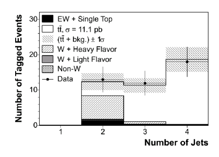
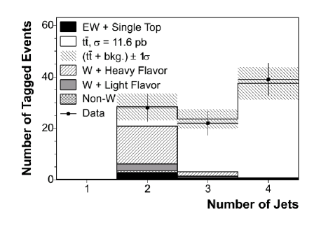
The statistical uncertainty on the measured cross section is dominated by the data sample size. Table 31 summarizes the systematic contributions to the cross section uncertainty.
| Source | Fractional Syst. Uncert. (%) | Contribution to (%) | |
|---|---|---|---|
| 1% | 5% | ||
| Central Electron ID | 1.6 | +0.98/-0.96 | +0.98/-0.96 |
| Central Muon ID | 1.9 | +0.60/-0.60 | +0.61/-0.60 |
| CMX Muon ID | 1.8 | +0.21/-0.21 | +0.21/-0.21 |
| 2 | +2.1/-2.0 | +2.1/-2.0 | |
| Jet Energy Scale | 4.2 | +4.5/-4.1 | +4.5/-4.1 |
| Lepton Isolation | 2 | +2.1/-2.0 | +2.1/-2.0 |
| ISR/FSR | 1.3 | +1.3/-1.3 | +1.3/-1.3 |
| MC Modeling | 1.6 | +1.7/-1.6 | +1.7/-1.6 |
| Z Vertex | 2.0 | +2.1/-2.0 | +2.1/-2.0 |
| Tagging 1% (b’s/c’s) | 8.6/12.9 | +20.3/-14.7 | — |
| Tagging 5% (b’s/c’s) | 8.5/12.7 | — | +18.3/-13.6 |
| Mistag Asymmetry 1% | 11.0 | +0.063/-0.063 | — |
| Mistag Asymmetry 5% | 15.5 | — | +0.44/-0.44 |
| Non-W Fraction | 50 | 0.060 | 0.092 |
| Non-W Prediction | 50 | 0.13 | 0.21 |
| W+HF Prediction | 30 | 0.84 | 1.0 |
| Cross Sections Bkg. | 1.8 | 0.027 | 0.030 |
| Luminosity | 5.9 | +6.4/-5.7 | +6.4/-5.7 |
| Total Systematic Uncertainty | +22.2/-16.8 | +20.4/-15.9 | |
IX.2 Cross Section Dependence on the Top Quark Mass
We study the dependence of the cross section using the double tag sample on the top quark mass in an analogous way to Section VIII.1. Results are shown in Fig. 22. A linear fit to the measured cross sections as a function of the top mass returns a slope of -0.096 0.022 pb/() and -0.082 0.019 pb/() for 1% and 5%, respectively, where the uncertainties are due to Monte Carlo simulation statistics. As before, note that the fit results for agree with the measured cross section within the 1.6% uncertainty estimated in Section VII due to different modeling in PYTHIA and HERWIG.
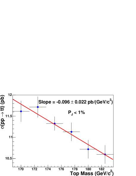
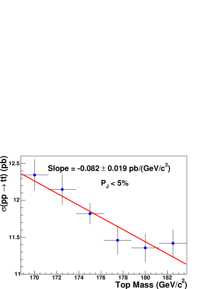
IX.3 Comparison Between Single and Double Tag Cross Sections
Although the measurements of the single and double tag cross sections are statistically compatible, we observe a ratio of about 1.2 between the measured cross sections in the double and single tag samples. We use pseudo-experiments to estimate the probability to obtain a cross section greater than the measured double tag cross section when we assume that the measured single tag cross section is correct. For each pseudo-experiment, we vary the total double tag background estimate according to a Gaussian distribution with a width equal to its uncertainty. Successively, we add the background to the expected signal by assuming the single tag cross section and we vary the total number of events according to a Poisson distribution. We repeat this procedure 10,000 times and count the number of pseudo-experiments in which we have a result greater than the one observed in data. We find a probability of 13.2% for 1% and 15.6% for 5%.
The systematic uncertainty in the double tag measurement is dominated by the uncertainties on the acceptance, luminosity and tagging scale factor. The systematic uncertainties on the background prediction are negligible. A bias on the values of acceptance and luminosity would affect the cross section measurement in the single and double tag samples in the same way. However, a bias on the tagging scale factor would have a greater effect in the double tag analysis than in the single tag one. To study this, we vary the tagging scale factor by and we repeat the cross section measurements and the pseudo-experiments. Results are summarized in Tables 32 and 33. As expected, the cross sections measured in the double tag sample are more sensitive to a change in the scale factor, resulting in a better agreement between the single and double tag cross sections when a larger value for the scale factor is used.
| - | + | ||
|---|---|---|---|
| 1%, 1 tag | |||
| 1%, 2 tags | |||
| 5%, 1 tag | |||
| 5%, 2 tags |
| - | + | ||
|---|---|---|---|
| 1% | 4.5% | 13.2% | 30% |
| 5% | 2.8% | 15.6% | 35% |
X Conclusions
We present a measurement of the production cross section in collisions at TeV with an integrated luminosity of 318 18 pb-1 at the CDF detector. We select events compatible with the decay mode by requiring one isolated electron (muon) with transverse energy and missing transverse energy and at least three jets with transverse energy . We further require at least one jet tagged by the jet probability algorithm. This selection accepts an estimated (3.5 0.3)% of all events when a 1% cut is applied, and an estimated (4.4 0.4)% with a looser cut at 5%. Backgrounds are estimated using data and Monte Carlo simulations. We find good agreement with the observed data in a control region defined by events with W+one or two jets. Using the excess of events with three or more jets and at least one tag with 1%, we measure a top pair production cross section of
As cross checks, we measure the cross section using samples with different -tagging requirements. Using events with at least one tag with 5% we obtain
We also measure the production cross section in events with at least two tagged jets. The acceptance for signal events is estimated to be (0.8 0.1)% for 1% and (1.5 0.3)% for 5%. We measure a cross section of
for 1% and
for 5%.
Figure 23 shows our main result together with other CDF cross section measurements and theoretical predictions. Our result is above the central theoretical value by 1.9 . It should be noted that our result is highly correlated with the lepton+jets measurement using secondary vertex -tagging, described in bib:secvtx_prl , where a comparison between the jet probability and secondary vertex -taggers is given.
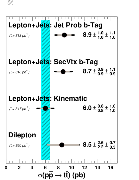
Acknowledgements.
We thank the Fermilab staff and the technical staffs of the participating institutions for their vital contributions. This work was supported by the U.S. Department of Energy and National Science Foundation; the Italian Istituto Nazionale di Fisica Nucleare; the Ministry of Education, Culture, Sports, Science and Technology of Japan; the Natural Sciences and Engineering Research Council of Canada; the National Science Council of the Republic of China; the Swiss National Science Foundation; the A.P. Sloan Foundation; the Bundesministerium für Bildung und Forschung, Germany; the Korean Science and Engineering Foundation and the Korean Research Foundation; the Particle Physics and Astronomy Research Council and the Royal Society, UK; the Russian Foundation for Basic Research; the Comisión Interministerial de Ciencia y Tecnología, Spain; the European Community’s Human Potential Programme under contract HPRN-CT-2002-00292; and the Academy of Finland.*
Appendix A Kinematic Distributions
We compare the distributions for different kinematic variables observed in data to the expectations for signal and backgrounds derived from a combination of simulation and cross section measurements. Figures 24 to 27 show the results for the four samples of events passing the selection criteria with at least three jets and one or two tags for 1% or 5%. The considered kinematic variables are the sum of the transverse energies of each object in the final state (), the reconstructed transverse mass of the boson, the missing transverse energy () of the event, the of the lepton, the transverse energy of the tagged jets, and the pseudo-rapidity of the tagged jets with respect to the center of the detector. Kolmogorov-Smirnov (KS) probabilities are computed to test the agreement between observed and expected distributions. The distributions observed in the data are statistically consistent with the expected signal-plus-background distributions.
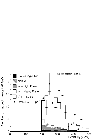
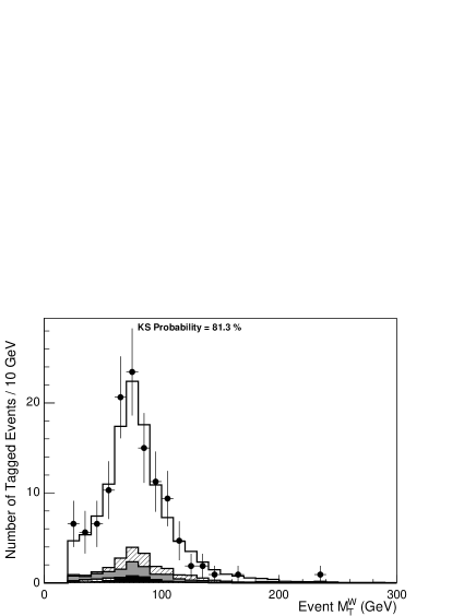

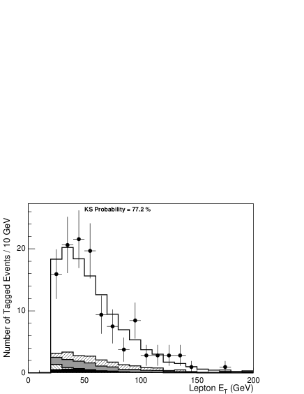


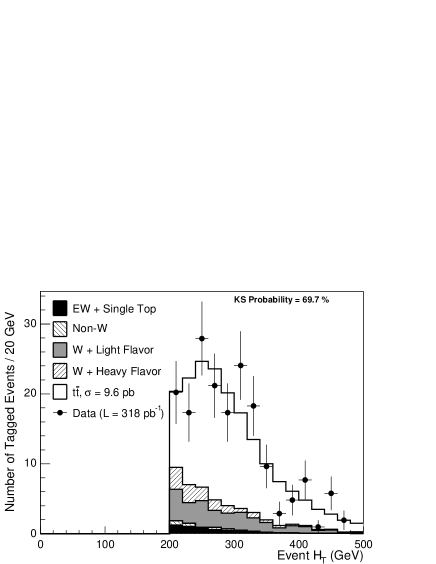


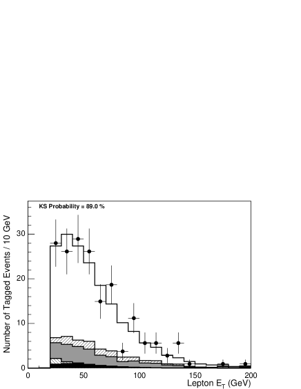

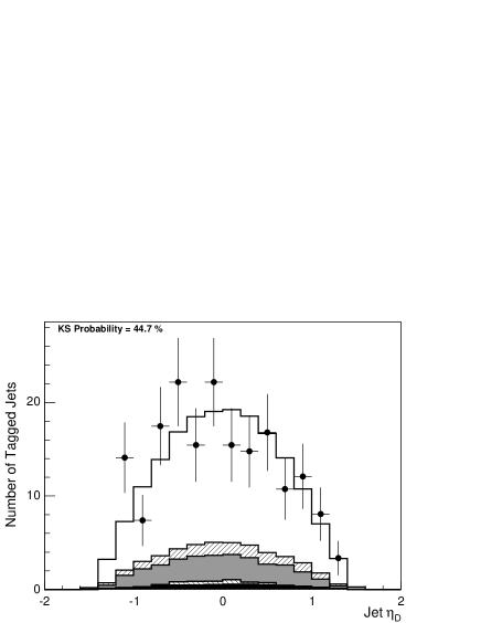
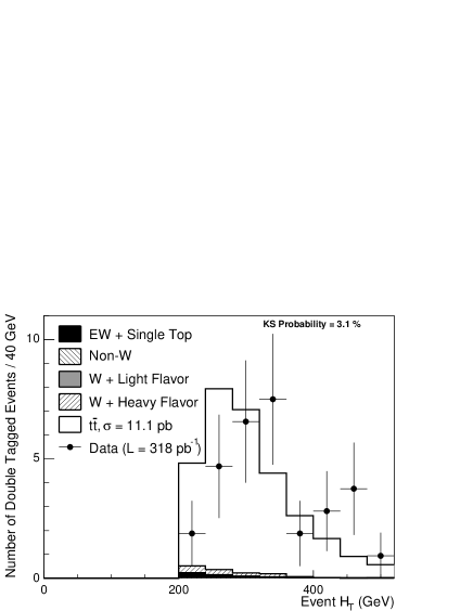
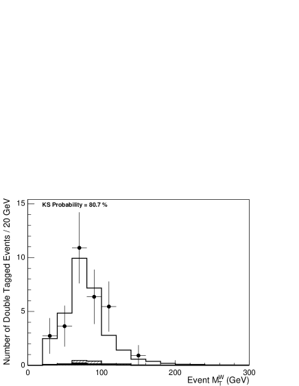


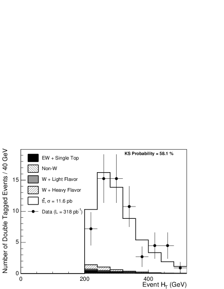

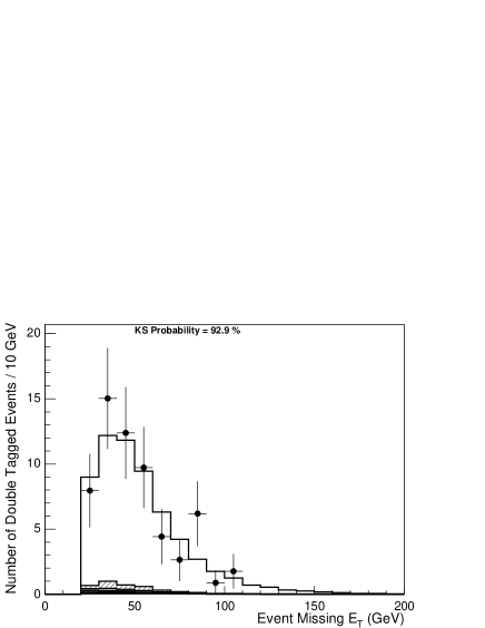

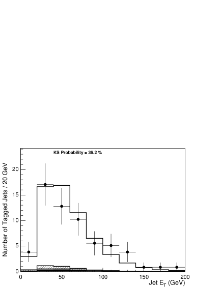
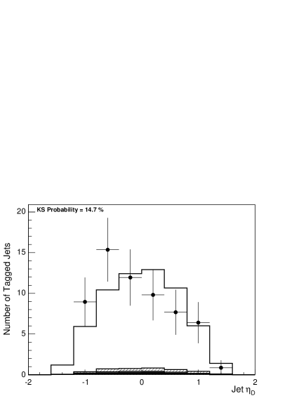
References
- (1) M. Cacciari, S. Frixione, G. Ridolfi, M. Mangano, and P. Nason, J. High Energy Phys. 0404, 068 (2004).
- (2) N. Kidonakis and R. Vogt, Phys. Rev. D 68, 114014 (2003).
- (3) P. Azzi et al. (CDF/DØ Collaborations), hep-ex/0404010.
-
(4)
A. Affolder et al. (CDF Collaboration), Phys. Rev. D 64, 032002 (2001), Erratum-ibid: Phys. Rev. D 67, 119901 (2003);
V.M. Abazov et al. (DØ Collaboration), Phys. Rev. D 67, 012004 (2003). - (5) D. Acosta et al. (CDF Collaboration), Phys. Rev. Lett. 93, 142001 (2004).
- (6) D. Acosta et al. (CDF Collaboration), Phys. Rev. D 71, 072005 (2005).
- (7) D. Acosta et al. (CDF Collaboration), Phys. Rev. D 71, 052003 (2005).
- (8) D. Acosta et al. (CDF Collaboration), Phys. Rev. D 72, 032002 (2005).
- (9) D. Acosta et al. (CDF Collaboration), Phys. Rev. D 72, 052003 (2005).
- (10) D. Acosta et al. (CDF Collaboration), Phys. Rev. D 71, 032001 (2005).
- (11) A. Affolder et al. (CDF Collaboration), Nucl. Instrum. Methods A 526, 249 (2004).
- (12) A. Sill et al. (CDF Collaboration), Nucl. Instrum. Methods A 447, 1 (2000).
- (13) A. Affolder et al. (CDF Collaboration), Nucl. Instrum. Methods A 453, 84 (2000).
- (14) L. Balka et al. (CDF Collaboration), Nucl. Instrum. Methods A 267, 272 (1988).
- (15) M. Albrow et al. (CDF Collaboration), Nucl. Instrum. Methods A 480, 524 (2002).
- (16) S. Bertolucci et al. (CDF Collaboration), Nucl. Instrum. Methods A 267, 301 (1988).
- (17) F. Abe et al. (CDF Collaboration), Phys. Rev. Lett. 68, 1104 (1992).
- (18) G. Ascoli et al., Nucl. Instrum. Methods A 268, 33 (1988).
- (19) T. Dorigo et al. (CDF Collaboration), Nucl. Instrum. Methods A 461, 560 (2001).
- (20) D. Acosta et al. (CDF Collaboration), Nucl. Instrum. Methods A 494, 57 (2002).
- (21) S. Klimenko, J. Konigsberg, and T.M. Liss, FERMILAB-FN-0741 (2003).
- (22) E. J. Thomson et al., IEEE Trans. Nucl. Sci. 49, 1063 (2002).
- (23) A. Abulencia et al. (CDF Collaboration), hep-ex/0508029.
- (24) F. Abe et al. (CDF Collaboration), Phys. Rev. D 45, 1448 (1992).
- (25) A. Bhatti et al., hep-ex/0510047, Fermilab-Pub-05-470.
- (26) T. Sjostrand et al., Comput. Phys. Commun. 135, 238 (2001).
- (27) G. Corcella et al., J. High Energy Phys. 0101, 010 (2001).
- (28) H.L. Lai et al. (CTEQ Collaboration), Eur. Phys. J C12, 375 (2000).
- (29) P. Avery, K. Read, and G. Trahern, CLEO Report CSN-212, 1985 (Unpublished).
- (30) M. Mangano et al., J. High Energy Phys. 0307, 001 (2003).
- (31) R. Brun and F. Carminati, CERN Programming Library Long Writeup W5013 1993.
- (32) R. Veenhof, Nucl. Instrum. Methods A 419, 726 (1998).
- (33) G. Grindhammer, M. Rudowitz, and S. Peters, Nucl. Instrum. Methods A 290, 469 (1990).
- (34) E. Gerchtein and M. Paulini, ECONF C0303241, TUMT005 (2003), physics/0306031.
-
(35)
D. Buskulic et al. (ALEPH Collaboration), Phys. Lett. B 313, 535 (1993);
F. Abe et al. (CDF Collaboration), Phys. Rev. D 53, 1051 (1996);
A. Affolder et al. (CDF Collaboration), Phys. Rev. D 64, 032002 (2001), Erratum-ibid: Phys. Rev. D 67, 119901 (2003) - (36) S. Eidelman et al. (Particle Data Group), Phys. Lett. B 592, 1 (2004).
- (37) J.M. Campbell et al., Phys. Rev. D 60, 113006 (2002).
- (38) B.W. Harris et al., Phys. Rev. D 66, 054024 (2002).
- (39) D. Acosta et al. (CDF Collaboration), Phys. Rev. Lett. 94, 091803 (2005).
- (40) A. Abulencia et al. (CDF Collaboration), hep-ex/0606017.
- (41) J. Guimaraes da Costa (CDF Collaboration), FERMILAB-PUB-05-593-E (2005).
- (42) In preparation, to be submitted to Phys. Rev. Lett.