First Observation of Quantum Interference in the Process $\phi\rightarrow$$K_{S}$$K_{L}$ $\rightarrow$ $\pi^{+}\pi^{-}$$\pi^{+}\pi^{-}$: a Test of Quantum Mechanics and $CPT$ Symmetry

Abstract

We present the first observation of quantum interference in the process $\phi$$\rightarrow$$K_{S}$$K_{L}$$\rightarrow$$\pi^{+}\pi^{-}$$\pi^{+}\pi^{-}$, using the KLOE detector at the Frascati $e^{+}e^{-}$ collider DAΦNE. From about $5\times 10^{4}$ neutral kaon pairs both decaying to $\pi^{+}\pi^{-}$ pairs we obtain the distribution of $\Delta t$, the difference between the two kaon decay times, which allows testing the validity of quantum mechanics and $CPT$ invariance: no violation of either is observed. New or improved limits on coherence loss and $CPT$ violation are presented.

, , , , , , , , , , , , , , , , , , , , , , , , , , , , , , , , , , , , , , , , , , , , , , , , , , , , , , , , , , , , , , , , , , , , , , , , , , , , , , , , , , , , , , , ,

¹ Corresponding author: Mario Antonelli, INFN - LNF, Casella postale 13, 00044 Frascati (Roma), Italy; tel. +39-06-94032728, e-mail mario.antonelli@lnf.infn.it

² Corresponding author: Antonio Di Domenico, Dipartimento di Fisica dell’Università “La Sapienza” e Sezione INFN, P.le A. Moro 2 00185 Roma, Italy; tel. +39-06-49914457, e-mail antonio.didomenico@roma1.infn.it

³ Corresponding author: Marianna Testa Dipartimento di Fisica dell’Università “La Sapienza” e Sezione INFN, P.le A. Moro 2 00185 Roma, Italy; tel. +39-06-49914614, e-mail marianna.testa@roma1.infn.it

1 Introduction

A $\phi$-factory provides unique opportunities for testing quantum mechanics (QM) and $CPT$ symmetry. In the decay $\phi\rightarrow K^{0}\bar{K}^{0}$, the neutral kaon pair is produced in a $J^{PC}=1^{--}$ state:

$$|\,i\rangle = {1\over\sqrt{2}}\>\left(|K^{0},\>{\bf p}\rangle|\bar{K}^{0},-{\bf p}\rangle-|\bar{K}^{0},\>{\bf p}\rangle|K^{0},\>-{\bf p}\rangle\right)$$ (1)

$$= {N\over\sqrt{2}}\>\left(|K_{S},\>{\bf p}\rangle|K_{L},-{\bf p}\rangle-|K_{L},\>{\bf p}\rangle|K_{S},\>-{\bf p}\rangle\right)$$

where p  is the kaon momentum in the $\phi$ meson rest frame, and $N=(1+|\epsilon|^{2})/(1-\epsilon^{2})$. Since $1-N\ll 1$ we will set $N=1$ in the following without any loss of generality. The decay intensity for the process $\phi$$\rightarrow$(2 neutral kaons)$\rightarrow$$\pi^{+}\pi^{-}$, $\pi^{+}\pi^{-}$ is then given by [1]:

$$I(t_{1},\ t_{2}) = \frac{1}{2}\>\left|\,\langle\pi^{+}\pi^{-}|\,K_{S}\rangle\,\right|^{\>4}\,\left|\,\eta_{+-}\right|^{\;2}\left(e^{-\Gamma_{L}t_{1}-\Gamma_{S}t_{2}}+e^{-\Gamma_{S}t_{1}-\Gamma_{L}t_{2}}\right.$$ (2)

$$\kern 56.9055pt\left.-2e^{-(\Gamma_{S}+\Gamma_{L})(t_{1}+t_{2})/2}\cos\,\left(\,\Delta m\,(t_{1}-t_{2})\,\right)\right)$$

where $t_{i}$ are the proper times of the two kaon decays, $\Gamma_{S}$ and $\Gamma_{L}$ are the decay widths of $K_{S}$ and $K_{L}$, $\Delta m=m_{L}-m_{S}$ is their mass difference and $\eta_{+-}=\langle\pi^{+}\pi^{-}|K_{L}\rangle/\langle\pi^{+}\pi^{-}|K_{S}\rangle=|\eta_{+-}|e^{i\phi_{+-}}$. The two kaons cannot decay into the same final state at the same time, even though the two decays are space-like separated events. Correlations of this type in QM were first pointed out by Einstein, Podolsky, and Rosen (EPR) [2].

While it is not obvious what a deviation from QM might be, the assumption that coherence is lost during the states time evolution does violate QM. One can therefore introduce a decoherence parameter $\zeta$ [3], simply multiplying the interference term in Eq. (2) by a factor of $(1-\zeta)$. The meaning and value of $\zeta$ depends on the basis in which the initial state (1) is written [4]. Eq. (2) is modified as follows:

$$I(\,t_{1},t_{2};\zeta_{SL}\,) = \frac{1}{2}\>\left|\,\langle\pi^{+}\pi^{-}|\,K_{S}\rangle\,\right|^{\>4}\,\left|\,\eta_{+-}\right|^{\;2}\left(e^{-\Gamma_{L}t_{1}-\Gamma_{S}t_{2}}+e^{-\Gamma_{S}t_{1}-\Gamma_{L}t_{2}}\right.$$ (3)

$$\kern 28.45274pt\left.-2\;(1-\zeta_{SL})\;e^{-(\Gamma_{S}+\Gamma_{L})(t_{1}+t_{2})/2}\cos\,\left(\,\Delta m\,(t_{1}-t_{2})\,\right)\right)$$

in the $K_{S}$-$K_{L}$ basis, and:

$$I(\,t_{1},t_{2};\zeta_{0\bar{0}}\,) = \frac{1}{2}\>\left|\,\langle\pi^{+}\pi^{-}|\,K_{S}\rangle\,\right|^{\>4}\,\left|\,\eta_{+-}\right|^{\;2}\left(e^{-\Gamma_{L}t_{1}-\Gamma_{S}t_{2}}+e^{-\Gamma_{S}t_{1}-\Gamma_{L}t_{2}}\right.$$ (4)

$$- 2e^{-(\Gamma_{S}+\Gamma_{L})(t_{1}+t_{2})/2}\cos\,\left(\,\Delta m\,(t_{1}-t_{2})\,\right)$$

$$+ \frac{\zeta_{0\bar{0}}}{2}\left(-e^{-\Gamma_{L}t_{1}-\Gamma_{S}t_{2}}-e^{-\Gamma_{S}t_{1}-\Gamma_{L}t_{2}}\right.$$

$$+ \left.2e^{-(\Gamma_{S}+\Gamma_{L})(t_{1}+t_{2})/2}\left(\cos\,\left(\,\Delta m(t_{1}-t_{2})\,\right)-\cos\,\left(\,\Delta m(t_{1}+t_{2})\,\right)\right)\right)$$

$$+ \left.\frac{1}{2}\frac{\zeta_{0\bar{0}}}{|\eta_{+-}|^{2}}\,e^{-\Gamma_{S}(t_{1}+t_{2})}\right)\quad\hbox{to the lowest order in $|\eta_{+-}|$ }$$

in the $K^{0}$-$\bar{K}^{0}$ basis.

Another phenomenological model [5] introduces decoherence via a dissipative term in the Liouville-von Neumann equation for the density matrix of the state and predicts decoherence to become stronger with increasing distance between the two kaons. This model introduces a parameter $\lambda$, related to the decoherence parameter in the $K_{S}$-$K_{L}$ basis by $\zeta_{SL}\simeq\lambda/\Gamma_{S}$.

In a hypothetical quantum gravity, space-time fluctuations at the Planck scale ($\sim$$10^{-33}$ cm), might induce a pure state to become mixed [6]. This results in QM and $CPT$ violation, changing therefore the decay time distribution of the $K^{0}$-$\hbox to0.0pt{\kern 3.00003pt\raise 8.1805pt\hbox to6.00006pt{\hrulefill}\hss}K\vphantom{K}^{0}$ pair from $\phi$ decays[7]. Three $CPT$- and QM-violating real parameters, with dimensions of mass, $\alpha,\beta$, and $\gamma$, are introduced in [7]. $\alpha,\beta$, and $\gamma$ are guessed to be of $\mathcal{O}(m_{K}^{2}/M_{P})\sim 2\times 10^{-20}$ GeV [7, 8], where $M_{P}=1/\sqrt{G_{N}}=1.22\times 10^{19}$ GeV is the Planck mass. The conditions $\alpha=\gamma$ and $\beta=0$ ensure complete positivity in this framework [9, 10, 11]. The decay intensity is (see Eq. (7.5) in Ref. [9] setting $\alpha=\gamma$ and $\beta=0$):

$$I(\,t_{1},t_{2};\gamma\,) = \frac{1}{2}\>\left|\,\langle\pi^{+}\pi^{-}|\,K_{S}\rangle\,\right|^{\>4}\,\left|\,\eta_{+-}\right|^{\;2}$$

$$\left(\left(1+\frac{\gamma}{\Delta\Gamma|\eta_{+-}|^{2}}\right)\left(e^{-\Gamma_{L}t_{1}-\Gamma_{S}t_{2}}+e^{-\Gamma_{S}t_{1}-\Gamma_{L}t_{2}}\right)\right.$$

$$- \left.2\cos\,\left(\,\Delta m\,(t_{1}-t_{2})\,\right)e^{-(\Gamma_{S}+\Gamma_{L})(t_{1}+t_{2})/2}-2\,\frac{\gamma}{\Delta\Gamma|\eta_{+-}|^{2}}e^{-\Gamma_{S}(t_{1}+t_{2})}\right)$$

It has been pointed out [12, 13] that in this context the initial state (1) may acquire a small $C$-even component:

$$|\,i\rangle = {1\over\sqrt{2}}\>\left(|K^{0},\>{\bf p}\rangle|\bar{K}^{0},-{\bf p}\rangle-|\bar{K}^{0},\>{\bf p}\rangle|K^{0},\>-{\bf p}\rangle\right.$$ (6)

$$+ \left.\omega\left(|K^{0},\>{\bf p}\rangle|\bar{K}^{0},-{\bf p}\rangle+|\bar{K}^{0},\>{\bf p}\rangle|K^{0},\>-{\bf p}\rangle\right)\right)$$

where $\omega=|\omega|e^{i\Omega}$ is a complex parameter describing $CPT$ violation, whose order of magnitude is expected to be at most $|\omega|\sim\sqrt{(m^{2}_{K}/M_{P})/\Delta\Gamma}\sim 10^{-3}$, with $\Delta\Gamma=\Gamma_{S}-\Gamma_{L}$. The decay intensity is (see Eq.(3.3) in Ref. [13] setting $\alpha,\beta,\gamma=0$):

$$I(\,t_{1},t_{2};\omega\,) = \frac{1}{2}\>\left|\,\langle\pi^{+}\pi^{-}|\,K_{S}\rangle\,\right|^{\>4}\,\left|\,\eta_{+-}\right|^{\;2}\left(e^{-\Gamma_{S}t_{1}-\Gamma_{L}t_{2}}+e^{-\Gamma_{L}t_{1}-\Gamma_{S}t_{2}}\right.$$ (7)

$$- 2\cos\,\left(\,\Delta\,m\,(t_{1}-t_{2})\,\right)e^{-(\Gamma_{S}+\Gamma_{L})(t_{1}+t_{2})/2}+\frac{|\omega|^{2}}{|\eta_{+-}|^{2}}e^{-\Gamma_{S}(t_{1}+t_{2})}$$

$$+ 2\frac{|\omega|}{|\eta_{+-}|}\left(\cos\,\left(\,\Delta\,m\,t_{2}-\phi_{+-}+\Omega\,\right)e^{-\Gamma_{S}t_{1}-(\Gamma_{S}+\Gamma_{L})t_{2}/2}\right.$$

$$- \left.\left.\cos\,\left(\,\Delta\,m\,t_{1}-\phi_{+-}+\Omega\,\right)e^{-\Gamma_{S}t_{2}-(\Gamma_{S}+\Gamma_{L})t_{1}/2}\right)\right)$$

The decoherence parameters $\zeta_{SL}$ and $\zeta_{0\bar{0}}$, have been found in the past to be compatible with zero, with uncertainties of 0.16 and 0.7, respectively, using CPLEAR data [4, 5, 14]. CPLEAR has also analyzed single neutral-kaon decays to measure the $\alpha$, $\beta$, and $\gamma$ parameters [15]. The values obtained for all three parameters are compatible with zero, with uncertainties of $2.8\times 10^{-17}\mbox{~{}GeV}$, $2.3\times 10^{-19}\mbox{~{}GeV}$, and $2.5\times 10^{-21}\mbox{~{}GeV}$, respectively. The parameter $\omega$ has never been measured.

In the following, the improved KLOE measurements of the $\zeta_{SL}$, $\zeta_{0\bar{0}}$, $\lambda$, $\gamma$, and $\omega$ parameters are presented. The analysis is based on data collected at DAΦNE in 2001–2002, corresponding to an integrated luminosity of $L\approx 380$ $\mathrm{pb}^{-1}$. DAΦNE, the Frascati $\phi$ factory, is an $e^{+}e^{-}$ collider operated at a center of mass energy $W=M$($\phi$)$\sim$1020 MeV. Electrons and positrons collide in the horizontal plane at an angle of $\pi$$-$25 mrad. $\phi$-mesons are produced with approximately 12 MeV/c momentum toward the rings center, along the $x$-axis. The $z$-axis is taken as the bisectrix of the two beams, the $y$-axis being vertical.

2 The KLOE detector

The KLOE detector consists of a large, cylindrical drift chamber (DC), surrounded by a lead/scintillating-fiber electromagnetic calorimeter (EMC). A superconducting coil around the calorimeter provides a 0.52 T field. The drift chamber [16] is 4 m in diameter and 3.3 m in length. The momentum resolution is $\sigma_{p_{\perp}}/p_{\perp}\approx 0.4\%$. Two-track vertices are reconstructed with a spatial resolution of $\sim$ 3 mm. The calorimeter [17] is divided into a barrel and two endcaps. It covers 98% of the solid angle. Cells close in time and space are grouped into calorimeter clusters. The energy and time resolutions for photons of energy $E$ are $\sigma_{E}/E=5.7\%/\sqrt{E\ {\rm(GeV)}}$ and $\sigma_{t}=57\ {\rm ps}/\sqrt{E\ {\rm(GeV)}}\oplus 100\ {\rm ps}$, respectively. The KLOE trigger [18] uses calorimeter and chamber information. For this analysis, only the calorimeter signals are used. Two energy deposits above threshold ($E>50$ MeV for the barrel and $E>150$ MeV for the endcaps) are required.

Kaon regeneration in the beam pipe is a non negligible disturbance. The beam pipe is spherical around the interaction point, with a radius of 10 cm. The walls of the beam pipe, 500 $\mu$m thick, are made of a 62%-beryllium/38%-aluminum alloy (AlBeMet$\circledR$162). A beryllium cylindrical tube of 4.4 cm radius and 50$\mu$m thick, coaxial with the beam, provides electrical continuity.

We only use runs satisfying basic quality criteria. For each run we determine the average collision conditions: p=p${}_{e^{+}}$+p${}_{e^{-}}$=p_ϕ, the center of mass energy W, the beam bunch dimensions, the collision point $\rm r$_C and angle. This is done using Bhabha scattering events. We then require $|p_{y,z}|<$ 3 MeV, $|W-1020|<$ 5 MeV. The collision point must satisfy $|\,x_{\rm C}\,|<$ 3 cm, $|\,y_{\rm C}\,|<$ 3 cm, and $|z_{\rm C}|<$ 5 cm. The rms spread of the luminous region must satisfy $\sigma_{x}<$ 3 cm and $\sigma_{z}<$ 3 cm. A small number of runs were rejected because of improper trigger operation. Each run used in the analysis is simulated with the KLOE Monte Carlo (MC) simulation program, GEANFI [19], using values of relevant machine parameters such as $W$ and p_ϕ determined as mentioned above. Machine background obtained from data is superimposed on MC events on a run-by-run basis. For $K_{S}$$K_{L}$$\rightarrow$$\pi^{+}\pi^{-}$$\pi^{+}\pi^{-}$ events, the number of simulated events is 10 times that expected on the basis of the integrated luminosity. For all other processes, the effective statistics of the simulated sample and of the data sample are approximately equal. The effects of initial- and final-state radiation are included in the simulation. Final-state radiation in $K_{S}$ and $K_{L}$ decays is treated as discussed in Ref. [20].

3 Analysis

3.1 Event selection

Events are selected on the basis of two identified neutral kaons from $\phi$ decay, in turn decaying into $\pi^{+}$$\pi^{-}$ pairs. Since we cannot tell whether $\pi^{+}\pi^{-}$ decays near the interaction point (IP) are from a $K_{S}$ or a $K_{L}$, we try to ensure that the same criteria are used for all decays. In the following we call $K_{1}$ ($K_{2}$) the decay closest to (farthest from) the $\phi$ production point.

We first require a $K_{1}$ vertex with two tracks of opposite curvature within a fiducial volume with $r<10$ cm and $|\,z\,|<20$ cm centered at the nominal collision point $\rm r$_C, determined as discussed above. We also require that the two tracks satisfy $|\,m_{\pi^{+}\pi^{-}}-m_{K}\,|<5$ MeV and $|\,p_{\pi^{+}\pi^{-}}-p_{K}\,|<$ 10 MeV/$c$, where $p_{K}$ is calculated from the kinematics of $\phi$$\rightarrow$$K_{S}$$K_{L}$. $m_{\pi^{+}\pi^{-}}$ and $p_{\pi^{+}\pi^{-}}$ are respectively the invariant mass and the momentum of the $\pi^{+}\pi^{-}$ pair.

In order to search for a second $\pi^{+}\pi^{-}$ kaon decay ($K_{2}$), all relevant tracks in the chamber—after removal of those originating from the decay already identified—are extrapolated to their points of closest approach to the $K_{2}$ path computed from kinematics and $\rm x$_C. For each track candidate we compute $d$, the distance of closest approach to the $K_{2}$ path. For each charge we take the tracks with smallest value of $d$ as the $K_{2}$ decay pions. We then determine the two track vertex and require that $|\,m_{\pi^{+}\pi^{-}}-m_{K}\,|<5$ MeV and $|\,p_{\pi^{+}\pi^{-}}-p_{K}\,|<$ 10 MeV/$c$. We also require $-$50$<E^{\,2}_{\rm miss}-p_{\rm miss}^{\,2}<10$ MeV${}^{\,{}^{2}}$ and $\sqrt{E^{\,2}_{\rm miss}+p_{\rm miss}^{\,2}}<10$ MeV, where $p$_miss and $E_{\rm miss}$ are the missing momentum and energy computed assuming $K_{2}$$\rightarrow$$\pi^{+}\pi^{-}$.

More accurate values for the $K_{1,2}$ vertex positions, $\bar{\mbox{\boldmath{$\rm r$}}}_{1,2}$ and the collision point, $\bar{\mbox{\boldmath{$\rm r$}}}_{\rm C}$, are obtained from a kinematical fit. The fit makes use of the constraint from the $K_{1}$ and $K_{2}$ directions $\mbox{\boldmath{$\rm n$}}_{1,2}$ defined by:

$$\mbox{\boldmath{$\rm n$}}_{1,2}=\frac{(\mbox{\boldmath{$\rm p$}}_{+}+\mbox{\boldmath{$\rm p$}}_{-})_{1,2}-(\mbox{\boldmath{$\rm p$}}_{+}+\mbox{\boldmath{$\rm p$}}_{-})_{2,1}+\mbox{\boldmath{$\rm p$}}_{\phi}}{|(\mbox{\boldmath{$\rm p$}}_{+}+\mbox{\boldmath{$\rm p$}}_{-})_{1,2}-(\mbox{\boldmath{$\rm p$}}_{+}+\mbox{\boldmath{$\rm p$}}_{-})_{2,1}+\mbox{\boldmath{$\rm p$}}_{\phi}|}.$$

We then have

$$\bar{\mbox{\boldmath{$\rm r$}}}_{i}=\bar{\mbox{\boldmath{$\rm r$}}}_{\rm C}+l_{i}\mbox{\boldmath{$\rm n$}}_{i},\qquad i=1,\ 2$$

and solve for $\bar{\mbox{\boldmath{$\rm r$}}}_{\rm C}$ and $l_{1,2}$ by maximizing the likelihood

$$\ln{\it L}=\sum_{i=1,2}\ln P_{i}(\mbox{\boldmath{$\rm r$}}_{i},\bar{\mbox{\boldmath{$\rm r$}}}_{\rm C}+l_{i}\mbox{\boldmath{$\rm n$}}_{i})+\ln P_{\rm C}(\mbox{\boldmath{$\rm r$}}_{\rm C},\bar{\mbox{\boldmath{$\rm r$}}}_{\rm C}),$$

where $P_{i}$ and $P_{\rm C}$ are the probability density functions for $\mbox{\boldmath{$\rm r$}}_{i}$ and $\mbox{\boldmath{$\rm r$}}_{\rm C}$, respectively, as obtained from MC. The value of $l_{1,2}$ has been kept positive in the maximization. The minimum of $-\ln{\it L}$ is shown in Fig. 1 for data and MC.

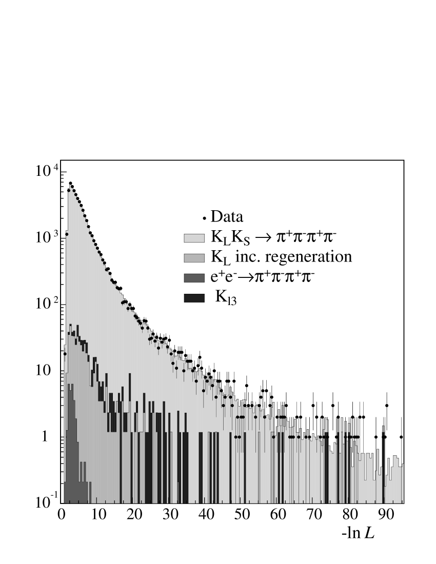
Figure 1: Distribution of the minimum of $-\ln{\it L}$ of the kinematic fit for data and Monte Carlo for different decay channels.

In order to maximize signal efficiency, improve $\Delta t$ resolution, and minimize incoherent regeneration background, as a final selection requirement we retain events with $-\ln{\it L}<7.5$.

The time difference between $K_{1}\rightarrow\pi^{+}\pi^{-}$ and $K_{2}\rightarrow\pi^{+}\pi^{-}$ is determined as $\Delta t=|t_{1}-t_{2}|$, where the proper time is $t_{i}=l_{i}/(\beta_{i}\gamma_{i})$ with $\beta_{i}\gamma_{i}=p_{K_{i}}/m_{K}$.

3.2 Determination of background

The selected $K_{S}K_{L}\rightarrow\pi^{+}\pi^{-}\pi^{+}\pi^{-}$ events have a contamination of $\sim$3.2% for $\Delta t<35\tau_{S}$ dominated by regeneration on the beam pipe. Semileptonic $K_{L}$ decays amount to $0.2\%$ as determined from MC. Direct four pion production, $e^{+}e^{-}\rightarrow\pi^{+}\pi^{-}\pi^{+}\pi^{-}$, gives a $\sim$0.3% contamination at the IP with $\Delta t\sim 0$, the region most sensitive to coherence loss. This contribution is obtained from the sidebands: $10\hbox{ MeV}<\sqrt{E^{2}_{\rm miss}+p_{\rm miss}^{2}}<20\hbox{ MeV}$ and $|p_{\pi^{+}\pi^{-}}-p_{K}|>1$ MeV. Vertex positions, total energy $E_{4\pi}$, and total momentum $p_{4\pi}$ are used to distinguish between $e^{+}e^{-}$$\rightarrow$$\pi^{+}\pi^{-}$$\pi^{+}\pi^{-}$ events and semileptonic $K_{L}$ decays near the IP. We find 27$\pm$8 events, in agreement with the estimate of $\sim$32 events from the cross section given in LABEL:cmd2:4pi.

Incoherent (see Sec. 3.4) and coherent regeneration on the beam-pipe are included in the fit of the $\Delta t$ distribution. The coherent regeneration amplitude, $\rho_{\rm coh}=|\rho_{\rm coh}|e^{i\phi_{\rm coh}}$, is obtained from the time distribution for $K_{L}(\rightarrow K_{S})\rightarrow\pi^{+}\pi^{-}$ decays after single $K_{L}$’s cross the beam pipe:

$$I(t) = \left|\langle\pi^{+}\pi^{-}|\,K_{L}(t)+\rho_{\rm coh}|K_{S}(t)\rangle\right|^{2}$$

$$= \left|\langle\pi^{+}\pi^{-}|K_{S}\rangle\right|^{2}\left(|\eta_{+-}|^{2}\,e^{-\Gamma_{L}t}+|\rho_{\rm coh}|^{2}e^{-\Gamma_{S}t}\right.$$

$$+ 2\left.|\eta_{+-}|\,|\rho_{\rm coh}|\,e^{-(\Gamma_{S}+\Gamma_{L})t/2}\cos(\Delta mt+\phi_{\rm coh}-\phi_{+-})\right)$$

$K_{L}$’s are identified by the reconstruction of a $K_{S}$$\rightarrow$$\pi^{+}\pi^{-}$ decay, using the same algorithm used for the measurement of the $K_{L}\rightarrow\pi^{+}\pi^{-}$ branching ratio [22]. In addition we require $|\,p_{K_{L}}-p_{\pi^{+}\pi^{-}}\,|<5$ MeV and $|E_{\pi^{+}\pi^{-}}-\sqrt{p_{K_{L}}^{2}+m_{K}^{2}}+m_{\pi^{+}\pi^{-}}-m_{K}|<5$ MeV, where the $K_{L}$ momentum, $p_{K_{L}}$, is obtained from the $K_{S}$ direction and p_ϕ and $E_{\pi^{+}\pi^{-}}$ is the energy of the $\pi^{+}\pi^{-}$ pair. These cuts are effective for the identification of $K_{L}$$\rightarrow$$\pi^{+}\pi^{-}$ decays and coherent and incoherent $K_{L}$$\rightarrow$$K_{S}$$\rightarrow$$\pi^{+}\pi^{-}$regeneration processes with a negligible amount of background. Incoherent regeneration is rejected by requiring that the angle between p${}_{K_{L}}$ and p${}_{\pi^{+}\pi^{-}}$ be smaller than 0.04. The residual contamination is $\sim$3%, from the sidebands of the distribution in the above angle. Fitting the proper-decay-time distribution, Eq. (3.2), we obtain $|\rho_{\rm coh}|=(6.5\pm 2.2)\times 10^{-4}$ and $\phi_{\rm coh}=(-1.05\pm 0.25)$ rad. This result is stable against variations of the scattering angle cut and agrees with predictions [23]. Coherent regeneration in the inner pipe is negligible. Background due to production of $C$-even neutral kaon pairs in two photon processes or $(f_{0},\ a_{0})$ decays is also negligible [24, 25, 26, 1].

3.3 Determination of the detection efficiency

The overall detection efficiency is about 30%, and has contributions from the event reconstruction and event selection efficiencies. These efficiencies have been evaluated from MC. For the reconstruction efficiency, a correction obtained from data is applied. This correction is determined using an independent sample of $K_{S}K_{L}\rightarrow\pi^{+}\pi^{-},\pi\mu\nu$ decays. $\pi\mu\nu$ decays are identified by requiring $\sqrt{E^{2}_{miss}+p_{\rm miss}^{2}}>$ 10 MeV, $|p^{*}_{\pm}|<246$ MeV and $p^{*}_{+}+p^{*}_{-}<367$ MeV, where $p^{*}$ is the momentum of the decay secondary in the kaon rest-frame, calculated assuming the $\pi$ mass hypothesis. We then compute the squared lepton mass $m^{2}_{l^{-}}$($m^{2}_{l^{+}}$) in the hypothesis $K\rightarrow\pi^{+}\mu^{-}\bar{\nu}$ ($K\rightarrow\pi^{-}\mu^{+}\nu$), and require: $150\,{\rm MeV}^{2}<m^{2}_{l^{-}}+m^{2}_{l^{+}}<270\,{\rm MeV}^{2}$. The distribution of the time difference $\Delta t=|t_{1}-t_{2}|$ between the two kaon decays obtained for the $K_{S}K_{L}\rightarrow\pi^{+}\pi^{-},\pi\mu\nu$ sample is shown in Fig. 2, both for data and MC.

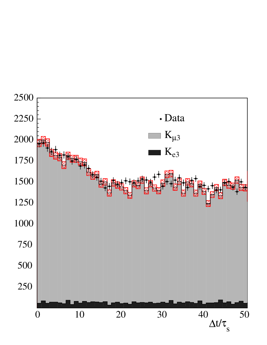
Figure 2: $\Delta t$ distribution for the $K_{S}K_{L}\rightarrow\pi^{+}\pi^{-},\pi\mu\nu$ control sample for data (black points) and Monte Carlo (solid histogram). The expected background contamination from $K_{S}K_{L}\rightarrow\pi^{+}\pi^{-},\pi e\nu$ is also shown. The hatched area represents the Monte Carlo statistical uncertainty.

The correction to the reconstruction efficiency from the MC is obtained from the data-MC ratio of the distributions in Fig. 2 and applied bin by bin as a function of $\Delta t$.

In order to take into account the $\Delta t$ resolution when fitting, a smearing matrix has been constructed from MC by filling a two-dimensional histogram with the “true” and reconstructed values of $\Delta t$. The efficiency correction and the smearing matrix are then used in the fit procedure as explained in the following section.

3.4 Fit

We fit the observed $\Delta t$ distribution between 0 and 35$\tau_{S}$ in intervals of $\overline{\Delta t}=\tau_{S}$. The fitting function is obtained from the $I(t_{1},t_{2})$ distribution given in Eq. (2) including the QM violating parameter $\zeta$, or the QM and $CPT$ violating parameters $\gamma$ and $\omega$ as discussed in Sec.1. To take coherent regeneration into account in Eq. (2), the time evolution of the single kaon is modified as follows:

$$|K_{S,L}(t_{i})\rangle=|K_{S,L}(t_{i})\rangle+\rho_{\rm coh}|K_{L,S}(t_{i})\rangle$$ (9)

where $\rho_{\rm coh}$ is evaluated as explained above. We then integrate $I(t_{1},t_{2})$ over the sum $t_{1}+t_{2}$ for fixed $\Delta t=|t_{1}-t_{2}|$, and over the bin-width of the data histogram:

$$I_{j}(\mbox{\boldmath{$\rm q$}})=\int_{(j-1)\bar{\Delta t}}^{j\bar{\Delta t}}\!\!d(\Delta t)\int_{\Delta t}^{\infty}{I(t_{1},t_{2};\mbox{\boldmath{$\rm q$}})}\>d(t_{1}+t_{2}),$$

where $\rm q$ is the vector of the QM- and $CPT$-violating parameters. Finally, the observed $\Delta t$ distribution is fitted with the following function:

$$n_{i}=N\left(\sum_{j}s_{ij}\>\epsilon_{j}\>I_{j}(\mbox{\boldmath{$\rm q$}})\right)+N^{\rm reg}I^{\rm reg}_{i}+N_{4\pi}{I_{4\pi,i}}$$ (10)

where $n_{i}$ is the expected number of events in the $i^{\rm th}$ bin of the histogram, $s_{ij}$ is the smearing matrix, and $\epsilon_{j}$ is the efficiency. $N$, the number of $K_{S}K_{L}\rightarrow\pi^{+}\pi^{-}\pi^{+}\pi^{-}$ events, and $N^{\rm reg}$, the number of events due to incoherent regeneration, are free parameters in the fit. The time distribution $I^{\rm reg}_{i}$ for the contribution from incoherent regeneration is evaluated from MC. The contribution from non-resonant $e^{+}e^{-}\rightarrow\pi^{+}\pi^{-}\pi^{+}\pi^{-}$ events is treated in a similar manner, except for that $N_{4\pi}$ is fixed to the value determined as in Sec. 3.2, rather than left free in the fit. The fit is performed by minimizing the least squares function:

$$\chi^{2} = \sum_{i=1}^{n}{(N_{i}^{\rm data}-n_{i})^{2}/\left(n_{i}+(n_{i}\delta\epsilon_{i}/\epsilon_{i})^{2}\right)}$$ (11)

where $N_{i}^{\rm data}$ is the number of events observed in the $i^{\rm th}$ bin and $\delta\epsilon_{i}$ is the error on the efficiency, including the correction. Using Eq. (10) with the QM- and $CPT$-violating parameters fixed to zero, $\Delta m$ can be left as free parameter and evaluated. In this case, the fit gives

$$\Delta m=(5.61\pm 0.33)\times 10^{9}\,\mbox{s}^{-1},$$

which is compatible with the more precise value given by the PDG [27]:

$$\Delta m=(5.290\pm 0.015)\times 10^{9}\,\mbox{s}^{-1}.$$

For the determination of the QM- and $CPT$-violating parameters, $\Delta m$ is fixed to the PDG value in all subsequent fits. As an example, the fit of the $\Delta t$ distribution used to determine $\zeta_{SL}$ is shown in Fig. 3: the peak in the vicinity of $\Delta t\sim 17\,\tau_{S}$ is due to coherent and incoherent regeneration on the spherical beam pipe.

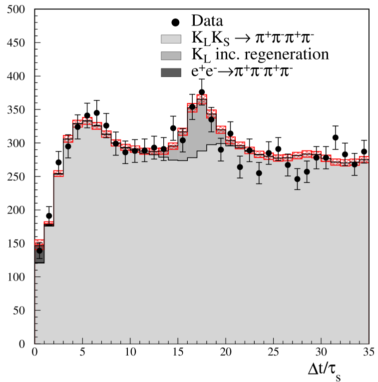
Figure 3: $\Delta t$ distribution from the fit used to determine $\zeta_{SL}$. The black points with errors are data and the solid histogram is the fit result. The uncertainty arising from the efficiency correction is shown as the hatched area.

3.5 Systematic uncertainties

As possible contributions to the systematic uncertainties on the QM- and $CPT$-violating parameters determined, we have considered the effects of data-MC discrepancies (in particular on the $\Delta t$ resolution), dependences on cut values, and imperfect knowledge of backgrounds and other input parameters. The contributions from each source to the systematic uncertainty on each parameter determined are summarized in Tab. 1, and discussed in further detail in the following.

Table 1: Summary of systematic uncertainties

	Cut	Resolution	Inputs	Coherent	$\pi^{+}\pi^{-}\pi^{+}\pi^{-}$
	stability			reg.	bckgnd
$\delta\,\zeta_{SL}$	0.007	0.002	0.001	0.001	0.020
$\delta\,\zeta_{0\bar{0}}\times 10^{5}$	0.03	0.01	0.01	-	0.11
$\delta\,\gamma\times 10^{21}$ GeV	0.4	0.2	0.1	0.3	1.3
$\delta$ $\Re\,\omega\times 10^{4}$	0.8	0.1	0.1	0.3	1.4
$\delta$ $\Im\,\omega\times 10^{4}$	0.4	0.4	0.2	0.3	0.1

Since the QM- and $CPT$- violating parameters are most sensitive to small values of $\Delta t$, particular attention has been devoted to the evaluation of systematic effects in that region. The dependence of the detection efficiency on $\Delta t$ is mostly due to the cut on $-\ln{\it L}$ in the kinematic fit used to evaluate the vertex positions. We have varied the cut from 6.5 to 8.5, corresponding to a fractional variation in the efficiency of $\sim 5\%$. The corresponding changes in the final results are consistent with statistical fluctuations. For each physical parameter determined, we take the systematic error from this source to be half of the difference between the highest and lowest parameter values obtained as a result of this study. These contributions are listed in the first column of Tab. 1.

The QM- and $CPT$-violating parameters depend also on the $\Delta t$ resolution. We have checked the reliability of the MC simulation on a sample of events with $K_{1}$=$K_{S}$ $K_{2}$=$K_{L}$ by requiring $l_{2}>12$ cm and removing the $l_{1}>0$ cut. Fig. 4 shows the $K_{S}$ proper-time distribution for data and MC. From the negative tail of the $K_{S}$ proper-time distribution we obtain the experimental resolution.

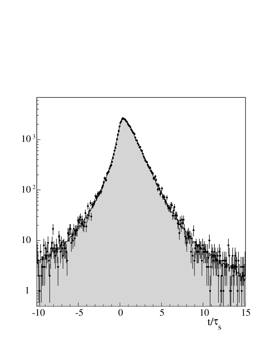
Figure 4: Distribution of $K_{S}$ proper-time distribution for data (black points) and Monte Carlo (solid histogram).

We fit the data and MC distributions to an exponential function convoluted with the resolution. We obtain an rms spread of $(1.152\pm 0.020)\,\tau_{S}$ for data and $(1.1807\pm 0.0036)\,\tau_{S}$ for MC, i.e., the data and MC resolutions agree to within 1.4 standard deviations. In addition, we obtain a $K_{S}$ lifetime, $\tau_{S}=(0.9030\pm 0.056)\,10^{-10}$ s, in agreement with the world average value $(0.8958\pm 0.0005)\,10^{-10}$ s [27]. To estimate the resulting contributions to the systematic uncertainties on the QM- and $CPT$-violating parameters, the MC resolution is varied by $\pm$5%, about three times the statistical uncertainty of the check. For each parameter determined, we take the systematic error from this source to be half of the difference between the highest and lowest values obtained. These contributions are listed in the second column of Tab. 1. The third column gives the contributions of uncertainties on the known values of $\Delta m$, $\Gamma_{L}$, $\Gamma_{S}$ and $\eta_{+-}$, which have been propagated numerically.

Contributions to the systematic uncertainties due to limited knowledge on $|\rho_{\rm coh}|$ and $\phi_{\rm coh}$ have been evaluated by varying the parameter values within their errors and are listed in the fourth column of Tab. 1.

Finally the last column gives the contributions arising from the uncertainty on the level of background contamination from non-resonant $e^{+}e^{-}\rightarrow\pi^{+}\pi^{-}\pi^{+}\pi^{-}$ events, evaluated by varying the background parameter in the fits ($N_{4\pi}$ in Eq. (10)) within its error. Note, however, that these contributions are included in the statistical uncertainties, rather than in the systematic uncertainties, in the statement of the final results.

4 Results and conclusions

From the fit we obtain the decoherence parameter values:

$$\zeta_{SL} = 0.018\,\pm 0.040_{\mbox{stat}}\pm 0.007_{\mbox{syst}}\qquad\qquad~{}~{}\chi^{2}/\mbox{dof}=29.7/32;$$

$$\zeta_{0\bar{0}} = \left(0.10\,\pm 0.21_{\mbox{stat}}\pm 0.04_{\mbox{syst}}\right)\times 10^{-5}\qquad\chi^{2}/\mbox{dof}=29.6/32.$$

which are consistent with $\zeta=0$ and no QM modification. Using the Neyman procedure[28], we derive the upper limits $\zeta_{SL}<0.098$ and $\zeta_{0\bar{0}}<0.50\times 10^{-5}$ at 95% C.L. Since decoherence in the $K^{0}\bar{K}^{0}$ basis would result in the $CP$ allowed $K_{S}K_{S}\rightarrow\pi^{+}\pi^{-}\pi^{+}\pi^{-}$ decays, Eq. 4, the value for $\zeta_{0\bar{0}}$ is naturally much smaller. In the model of LABEL:bertlmann2, we find:

$$\lambda=(0.13\pm 0.30_{\mbox{stat}}\pm 0.05_{\mbox{syst}})\times 10^{-15}\ \mbox{GeV},\quad\lambda<0.73\times 10^{-15}\ \mbox{GeV at 95\% C.L.}.$$

All the above results are a considerable improvement on those obtained from CPLEAR data [4, 5]. We have measured the $\gamma$ parameter:

$$\gamma=\left(1.3^{+2.8}_{-2.4}\pm 0.4\right)\times 10^{-21}\,\mbox{GeV}$$

with $\chi^{2}/\mbox{dof}=33/32$. From the above we find $\gamma<6.4\times 10^{-21}\,\mbox{GeV}$ at 95 % C.L.. This result is competitive with that obtained by CPLEAR [15] using single kaon beams.

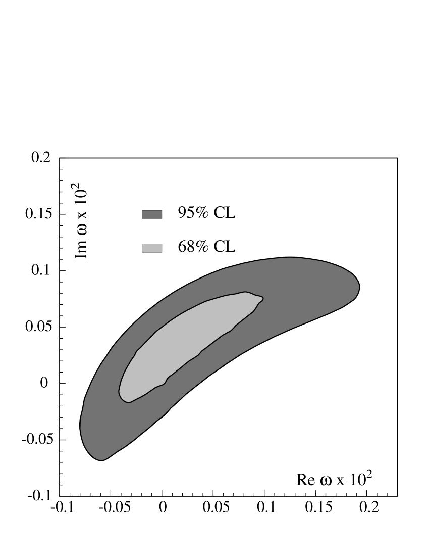
Figure 5: Contour plot of $\Im\,\omega$ versus $\Re\,\omega$ at 68% and 95% C.L.

The complex parameter $\omega$ has been measured for the first time. The result is

$$\Re\,\omega=\left(1.1^{+8.7}_{-5.3}\pm 0.9\right)\times{10^{-4}}\qquad\Im\,\omega=\left(3.4^{+4.8}_{-5.0}\pm 0.6\right)\times{10^{-4}}$$

with $\chi^{2}/\mbox{dof}=29/31$. The correlation coefficient between ${\Re\,\omega}$ and ${\Im\,\omega}$ is 90%. Fig. 5 gives the 68% and 95% C.L. contours in the $\Im\,\omega,\ \Re\,\omega$ plane. The upper limit is $|\omega|<2.1\times 10^{-3}$ at 95% C.L.

We do not find any evidence for QM or $CPT$ violation.

References

[1]I. Dunietz, J. Hauser, J. L. Rosner, Phys. Rev. D 35, (1987) 2166
[2] A. Einstein, B. Podolsky, N. Rosen, Phys. Rev.47, (1934) 777
[3] P.H. Eberhard, “Tests of Quantum Mechanics at a factory” in The second Dane handbook, Vol.I,
ed. L. Maiani, G. Pancheri, N. Paver, (1995) 99
[4] R. A. Bertlmann, W. Grimus, B. C. Hiesmayr, Phys. Rev. D 60, (1999) 114032
[5] R. A. Bertlmann, K. Durstberger, B. C. Hiesmayr,
Phys. Rev. A 68, (2003) 012111
[6] S. Hawking, Commun. Math. Phys.87 (1982) 395
[7] J. Ellis, J. S. Hagelin, D. V. Nanopoulos, M. Srednicki, Nucl. Phys. B 241, (1984) 381
[8] J. Ellis, J. L. Lopez, N. .E. Mavromatos, D. V. Nanopoulos, Phys. Rev. D 53, (1996) 3846
[9] P. Huet, M. Peskin, Nucl. Phys. B 434, (1995) 3
[10] F. Benatti, R. Floreanini, Nucl. Phys. B 511, (1998) 550
[11] F. Benatti, R. Floreanini, Phys. Lett. B 468, (1999) 287
[12] J. Bernabeu, N. Mavromatos, J. Papavassiliou, Phys. Rev. Lett.92, (2004) 131601
[13] J. Bernabeu, N. Mavromatos, J. Papavassiliou, A. Waldron-Lauda, Nucl. Phys. B 744, (2006) 180
[14] A. Apostolakis et al., CPLEAR Collaboration, Phys. Lett. B 422, (1998) 339
[15] R. Adler et al., CPLEAR Collaboration, Phys. Lett. B 364, (1995) 239
[16]
M. Adinolfi et al., KLOE Collaboration, Nucl. Instrum. Methods A 488, (2002) 51
[17]
M. Adinolfi et al., KLOE Collaboration, Nucl. Instrum. Methods A 482, (2002) 364
[18]
M. Adinolfi et al., KLOE Collaboration, Nucl. Instrum. Methods A 492, (2002) 134
[19]
F. Ambrosino et al., KLOE Collaboration, Nucl. Instrum. Methods A 534, (2004) 403
[20]
C. Gatti, Eur. Phys. J. C 45, (2006) 417
[21] R.R. Akhmetshin et al., Phys. Lett. B 595, (2004) 101
[22] F. Ambrosino et al., KLOE Collaboration, Phys. Lett. B 638, (2006) 140
[23] A. Di Domenico, Nucl. Phys. B 450, (1995) 293
[24] J. A. Oller, Nucl. Phys. A 714, (2003) 161
[25] N.N. Achasov, V. V. Gubin, Phys. Rev. D 64, (2001) 094016
[26] N.N. Achasov, V. V. Gubin, Phys. Atom. Nucl.65, (2002) 1887
[27] W.-M. Yao et al., Particle Data Group, J. Phys. G 33, (2006) 1
[28]G.J. Feldman, R. Cousins, Phys. Rev. D 57, (1998) 3873