Power Corrections in Electron-Positron Annihilation: Experimental Review

Abstract

Experimental studies of power corrections with $\mathrm{e^{+}e^{-}}$ data are reviewed. An overview of the available data for jet and event shape observables is given and recent analyses based on the Dokshitzer-Marchesini-Webber (DMW) model of power corrections are summarised. The studies involve both distributions of the observables and their mean values. The agreement between perturbative QCD combined with DMW power corrections and the data is generally good, and the few exceptions are discussed. The use of low energy data sets highlights deficiencies in the existing calculations for some observables. A study of the finiteness of the physical strong coupling at low energies using hadronic $\tau$ decays is shown.

I INTRODUCTION

Data from hadron production in $\mathrm{e^{+}e^{-}}$ annihilation experiments has been one of the main sources of experimental information for the study of non-perturbative QCD of hadron jets, see e.g. kluth06 ; dasgupta03 ; kluth01a ; kluth01b . Compared to other processes where power corrections have been studied such as hadron production in deep inelastic lepton-nucleon scattering dasgupta03 there are two main advantages:

Leptonic initial state

The incoming electron and positron are leptons and thus there is no interference between initial state and the hadronic final state. This makes the interpretation of of the final state in terms of QCD much more robust.

Large range of energies

The currently available data from $\mathrm{e^{+}e^{-}}$ annihilation to hadrons span a range of centre-of-mass (cms) energies of more than an order of magnitude. Since many effects in QCD depend on the energy scale comparing data sets recorded at different cms energies yields strong tests of the theory.

From reconstructed hadronic final states jet production or event shape observables are calculated, see e.q. dasgupta03 ; kluth06 . As an example the observable Thrust $T$ is defined by $T=\max_{\vec{n}}(\sum_{i}|\vec{n}\cdot\vec{p}_{i}|)/(\sum_{i}|\vec{p}_{i}|)$ where $\vec{p}_{i}$ is the 3-momentum of particle $i$ and $|\vec{n}|=1$. A value of $T=1$ corresponds to an ideal 2-jet event, events with three final state objects have $1>T>2/3$ while completely spherical events with many final state particles can approach $T=0.5$. Event shape observables $y$ are conventionally defined to have $y=0$ for ideal two-jet configurations and thus the Thrust is often analysed in terms of $1-T$. The observables can be classified as 3-jet or 4-jet observables depending on whether $y>0$ occurs in the cms for final states with $\geq 3$ or $\geq 4$ objects.

I.1 Experiments

The energy of the electron and electron beams in most $\mathrm{e^{+}e^{-}}$ annihilation collider experiments is equal due to the simplified construction and operation of a circular accelerator with only one beam line. As a consequence the cms of hadronic final states produced in $\mathrm{e^{+}e^{-}}$ annihilation coincides with the laboratory system in the absence of hard initial state radiation (ISR).

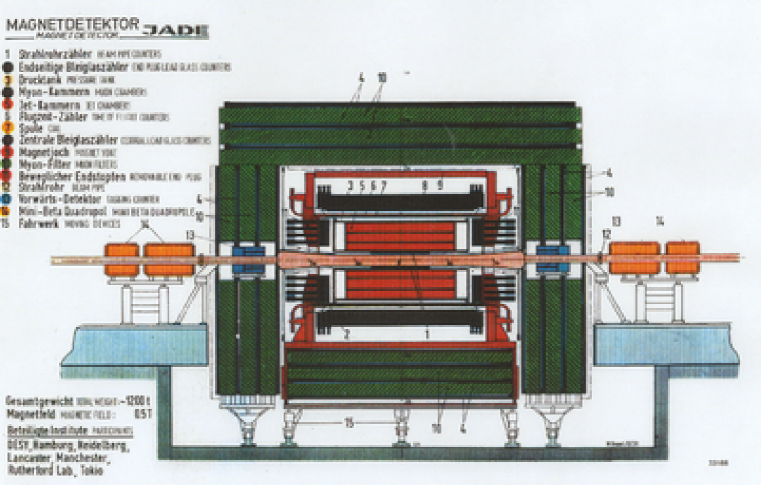
A typical $\mathrm{e^{+}e^{-}}$ annihilation experiment is shown in figure 1. The JADE detector (for details see naroska87 ) was operated at the PETRA accelerator petra80 from 1979 to 1986 at cms energies $12<\sqrt{s}<46.8$ GeV. The design of the experiment is similar to the more recent LEP experiments. The interaction region, where the electron and positron beams collide, is surrounded by gaseous tracking detectors (Jet Chamber) inside a solenoidal magnetic field of 0.48 T. The tracking detectors are inside a calorimeter consisting of 2712 lead glass blocks to measure the energy of charged and neutral particles. Tracking and calorimeter efficiency is good in the region $|\cos\theta|<0.97$ were $\theta$ is the angle w.r.t. the beam axis. Therefore most $\mathrm{e^{+}e^{-}}$ annihilation events are fully contained in the detector and complete reconstruction with high efficiency and good precision is possible. This reduces the size of experimental corrections for acceptance and resolution and thus the corresponding experimental uncertainties.

Figure 1: Drawing of the JADE experiment. The electron and positron beam come from the left and right and collide in the centre of the experiment.

I.2 Overview of data

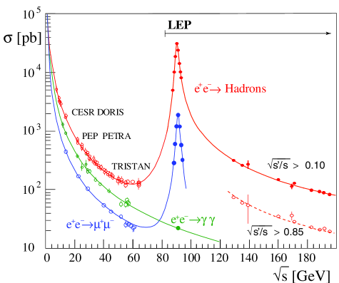
The experimental conditions vary significantly between the various cms energies of the data sets. Figure 2 (left) bethke00b shows the measured cross sections of several $\mathrm{e^{+}e^{-}}$ annihilation processes as a function of the cms energy $\sqrt{s}$. The $1/s$ dependence as expected from QED at low $\sqrt{s}$ is clearly visible. At the $\mathrm{Z^{0}}$ peak around $\sqrt{s}=91$ GeV the cross sections increase by a factor of about 100 compared to their lowest values at $\sqrt{s}\simeq 60$ GeV or $\sqrt{s}>130$ GeV.

At $\sqrt{s}<m_{\mathrm{Z^{0}}}$ background from two-photon interactions with hadronic final states ($\mathrm{e^{+}e^{-}}\rightarrow\gamma\gamma$), from production of $\tau$-lepton pairs decaying to hadrons and from hadronic final states with ISR and thus reduced cms is significant. Requiring more than four tracks of charged particles (events with exactly four tracks not in a 1- vs 3-prong configuration may also be accepted OPALPR299 ) reduces the backgrounds from $\tau$-pairs and two-photon interactions to negligible levels. The data collected on or near the $\mathrm{Z^{0}}$ peak are essentially free of backgrounds due to the high energy and large cross section. ISR effects are also suppressed. The high energy samples taken by the LEP experiments during the LEP 2 phase have again backgrounds from two-photon interactions, ISR and for $\sqrt{s}>2m_{\mathrm{W}}\simeq 161$ GeV from production of four-fermion final states dominated by $\mathrm{W^{+}W^{-}}$ pairs decaying to hadrons.

Figure 2: (left) Cross sections of several $\mathrm{e^{+}e^{-}}$ annihilation processes as indicated bethke00b . The lines represent theoretical predictions. The accelerators where the data where recorded are also shown. The variable $s^{\prime}$ refers to reduced cms energy after ISR. (right) Distribution of event shape observable Thrust $T$ measured at $\sqrt{s}\simeq 189$ GeV l3290 . The lines and hatched regions represent the predictions from Monte Carlo simulations of signal and background.

As a representative example figure 2 (right) shows the distribution of the event shape observable Thrust $T$ measured by L3 at $\sqrt{s}\simeq 189$ GeV l3290 . The simulation of signal and background samples shown in the figure agrees well with the data. The selection efficiency is $\epsilon\approx 90$% and the purity of the samples is about $p\approx 80$% l3290 . The remaining fraction of background from four-fermion events in the OPAL analysis OPALPR404 is 2.1% at 161 GeV and 6.2% at 207 GeV.

The experimental corrections are typically ${\cal O}(10)$% except at the edges of phase space. They reach values of 50% only for the LEP 2 samples because of the reduced selection efficiency of multi-jet final states due to the additional cuts to suppress four-fermion events.

Some 3-jet observables have had QCD predictions in next-to-leading order (NLO) combined with next-to-leading-log-approximation (NLLA) predictions ($1-T$, $M_{H}$, $B_{T}$, $B_{W}$, $C$, $y_{23}^{\mathrm{D}}$). Most power correction calculations are only available for these observables or a subset thereof. The final LEP results are l3290 ; aleph265 ; OPALPR404 ; delphi327 while many older measurements are summarised in colrun . Moments up to the order 5 of these and several other observables are also available OPALPR404 . The 4-jet observables $D$, $B_{N}$, $M_{L}$, $T_{\mathrm{min.}}$ and $y_{34}^{\mathrm{D}}$ were measured by OPAL and partially by L3 OPALPR404 ; l3290 .

II TRADITIONAL DMW STUDIES

The power correction model of Dokshitzer, Marchesini and Webber (DMW) extracts the structure of power correction terms from analysis of infrared renormalon contributions dokshitzer95a . Earlier versions of the model are webber94 ; dokshitzer95 . The model assumes that a non-perturbative strong coupling $\alpha_{\mathrm{S}}^{\mathrm{NP}}$ exists around and below the Landau pole and that the quantity $\alpha_{0}(\mu_{\mathrm{I}})=1/\mu_{\mathrm{I}}\int_{0}^{\mu_{\mathrm{I}}}\alpha_{\mathrm{S}}^{\mathrm{NP}}(k)\mathrm{d}k$ can be defined. The value of $\mu_{\mathrm{I}}$ is chosen to be safely within the perturbative region, usually $\mu_{\mathrm{I}}=2$ GeV. A study of the branching ratio of hadronic to leptonic $\tau$ lepton decays as a function of the invariant mass of the hadronic final state supports the assumption that the physical strong coupling is finite and thus integrable at low energy scales brodsky03 , see below.

The main result for the effects of power corrections on distributions $F(y)$ of the event shape observables $1-T$, $M_{H}$ and $C$ is that the perturbative prediction $F_{\mathrm{PT}}(y)$ is shifted dokshitzer97a ; dokshitzer98b ; dokshitzer99a :

$$F(y)=F_{\mathrm{PT}}(y-c_{\mathrm{y}}P)$$ (1)

where $c_{\mathrm{y}}$ is an observable dependent constant and $P\sim M\mu_{\mathrm{I}}/Q(\alpha_{0}(\mu_{\mathrm{I}})-\alpha_{\mathrm{S}})$ is universal, i.e. independent of the observable dokshitzer98b . The factor $P$ contains the $1/Q=1/\sqrt{s}$ scaling and the so-called Milan-factor $M=1.49$ for $n_{f}=3$ which takes two-loop effects into account. The non-perturbative parameter $\alpha_{0}$ is explicitly matched with the perturbative strong coupling $\alpha_{\mathrm{S}}$. For the event shape observables $B_{T}$ and $B_{W}$ the predictions are more involved and the shape of the pQCD prediction is modified in addition to the shift dokshitzer99a . For mean values of $1-T$, $M_{H}$ and $C$ the prediction is:

$$\mbox{$\langle y\rangle$}=\mbox{$\langle y\rangle$}_{\mathrm{PT}}+c_{\mathrm{y}}P$$ (2)

For $\langle B_{T}\rangle$ and $\langle B_{W}\rangle$ the predictions are also more involved due to the modification of the shape of the distributions.

Figure 3 (left) shows the results of fits to data for mean values of event shape observables measured over a large range of cms energies aleph265 . The perturbative QCD prediction in NLO $\mbox{$\langle y\rangle$}_{\mathrm{PT}}$ is combined with the power correction calculations as explained above. The combined prediction describes the available data well within the uncertainties even at low cms energies where non-perturbative effects are large. The numerical results are shown in table 1. The dashed lines show as a comparison the results of fits of the same NLO QCD predictions with Monte Carlo based hadronisation corrections. The data are also well described but the difference in values of $\alpha_{\mathrm{S}}(m_{\mathrm{Z^{0}}})$ for the same observables is about 6% aleph265 .

Figure 3: (left) Mean values of event shape observables as indicated aleph265 . The solid lines are fits of NLO QCD predictions combined with power corrections, the dashed lines present fits of the same NLO QCD predictions with Monte Carlo based hadronisation corrections. (right) Measurements of EEC at various $\sqrt{s}$ points as indicated delphi296 . The solid and dotted lines show the fitted QCD prediction including power corrections using only data points within the solid lines for the fit. The dashed lines present the same fit after subtraction of the power correction.

Figure 3 (right) shows data of the event shape observable EEC measured by DELPHI delphi296 over a large range of cms energies. Superimposed are fits of the perturbative QCD prediction in NLO+NLLA combined with power correction calculations dokshitzer99c . The distribution of EEC is sensitive to a higher order non-perturbative parameter referred to as $\alpha_{1}$. A fit with the three parameters $\alpha_{\mathrm{S}}(m_{\mathrm{Z^{0}}})$, $\alpha_{0}(2~{}\mathrm{GeV})$ and $\alpha_{1}(2~{}\mathrm{GeV})$ results in $\alpha_{\mathrm{S}}(m_{\mathrm{Z^{0}}})=0.117\pm 0.002$, $\alpha_{0}(2~{}\mathrm{GeV})=0.48\pm 0.05$ and $\alpha_{1}(2~{}\mathrm{GeV})=0.00\pm 0.04$. The results for $\alpha_{\mathrm{S}}(m_{\mathrm{Z^{0}}})$ and $\alpha_{0}(2~{}\mathrm{GeV})$ are consistent but the result for $\alpha_{1}(2~{}\mathrm{GeV})$ is not in agreement with an expectation $\alpha_{1}(2~{}\mathrm{GeV})=0.45$ from dokshitzer99c .

	Exp.	ALEPH aleph265	DELPHI delphi296	L3 l3290	MPI powcor
$\sqrt{s}$ range [GeV]		12(35)–206	12–202	41–206	12(35)–189
	$\alpha_{\mathrm{S}}(m_{\mathrm{Z^{0}}})$	$0.1207\pm 0.0019$	$0.1241\pm 0.0034$	$0.1164\pm 0.0060$	$0.1217\pm 0.0060$
1-T	$\alpha_{0}(2~{}\mathrm{GeV})$	$0.539\pm 0.011$	$0.491\pm 0.018$	$0.518\pm 0.059$	$0.528\pm 0.064$
	$\chi^{2}/\mathrm{d.o.f.}$	69/43	27/41	18/14	50/41
	$\alpha_{\mathrm{S}}(m_{\mathrm{Z^{0}}})$	$0.1161\pm 0.0018$	$0.1197\pm 0.0122$	$0.1051\pm 0.0051$	$0.1165\pm 0.0043$
$M_{H}$, $\rho$	$\alpha_{0}(2~{}\mathrm{GeV})$	$0.627\pm 0.020$	$0.339\pm 0.263$	$0.421\pm 0.037$	$0.663\pm 0.095$
	$\chi^{2}/\mathrm{d.o.f.}$	50/40	10/15	13/14	24/35
	$\alpha_{\mathrm{S}}(m_{\mathrm{Z^{0}}})$	$0.1148\pm 0.0025$	$0.1174\pm 0.0029$	$0.1163\pm 0.0042$	$0.1205\pm 0.0049$
$B_{T}$	$\alpha_{0}(2~{}\mathrm{GeV})$	$0.492\pm 0.020$	$0.463\pm 0.033$	$0.449\pm 0.054$	$0.445\pm 0.054$
	$\chi^{2}/\mathrm{d.o.f.}$	7/18	9/23	9/14	24/28
	$\alpha_{\mathrm{S}}(m_{\mathrm{Z^{0}}})$	$0.1179\pm 0.0028$	$0.1167\pm 0.0019$	$0.1169\pm 0.0042$	$0.1178\pm 0.0025$
$B_{W}$	$\alpha_{0}(2~{}\mathrm{GeV})$	$0.467\pm 0.037$	$0.438\pm 0.049$	$0.342\pm 0.079$	$0.425\pm 0.097$
	$\chi^{2}/\mathrm{d.o.f.}$	11/18	10/23	14/14	10/29
	$\alpha_{\mathrm{S}}(m_{\mathrm{Z^{0}}})$	$0.1228\pm 0.0027$	$0.1222\pm 0.0036$	$0.1164\pm 0.0047$	$0.1218\pm 0.0059$
$C$	$\alpha_{0}(2~{}\mathrm{GeV})$	$0.461\pm 0.016$	$0.444\pm 0.022$	$0.457\pm 0.040$	$0.461\pm 0.048$
	$\chi^{2}/\mathrm{d.o.f.}$	17/18	12/23	12/14	18/26
	$\alpha_{\mathrm{S}}(m_{\mathrm{Z^{0}}})$			$0.1046\pm 0.0124$
$D$	$\alpha_{0}(2~{}\mathrm{GeV})$	$--$	$--$	$0.682\pm 0.096$	$--$
	$\chi^{2}/\mathrm{d.o.f.}$			24/14

Table 1: Results for $\alpha_{\mathrm{S}}(m_{\mathrm{Z^{0}}})$ and $\alpha_{0}(2~{}\mathrm{GeV})$ from the analysis of mean values in the DMW power correction model. The errors consist of statistical and experimental uncertainties only for ALEPH and DELPHI and include also theoretical uncertainties for L3 and MPI.

Tables 1 and 2 summarise all recently published results from studies of DMW power correction using mean values and distributions of event shape observables. The values for $\alpha_{\mathrm{S}}(m_{\mathrm{Z^{0}}})$ and $\alpha_{0}(2~{}\mathrm{GeV})$ are generally consistent with each other except for the following observations:

• The values for $\alpha_{0}(2~{}\mathrm{GeV})$ from $M_{H}$ or $\rho$ are comparatively large. This is partially due to the effects of neglected hadron masses salam01a . The results from DELPHI take hadron masses into account according to salam01a and their values for $\alpha_{0}(2~{}\mathrm{GeV})$ are lower.

• The results for $\alpha_{0}(2~{}\mathrm{GeV})$ from distributions of $B_{T}$ and $B_{W}$ from DELPHI appear inconsistent with the other results as noted already in aleph265 .

• The results for $\alpha_{0}(2~{}\mathrm{GeV})$ are consistent at the level of 20 to 30% but the errors including theoretical effects are partially smaller and are about 10% in the case of the MPI analysis of mean values. The Milan factor $M$ has a theoretical uncertainty of about 20% dokshitzer98b . However, it is not clear if this uncertainty should be reflected in differing values of $\alpha_{0}(2~{}\mathrm{GeV})$ from different observables.

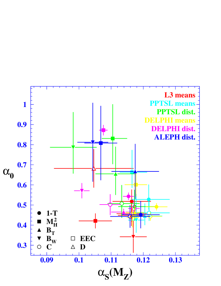
The correlations between the two parameters $\alpha_{\mathrm{S}}(m_{\mathrm{Z^{0}}})$ and $\alpha_{0}(2~{}\mathrm{GeV})$ are about $-90$% from the fits and between about $-40\%$ and 0% when systematic effects are considered. The results are also shown in figure 4. The negative correlation between $\alpha_{\mathrm{S}}(m_{\mathrm{Z^{0}}})$ and $\alpha_{0}(2~{}\mathrm{GeV})$ is visible in the figure.

	Exp.	ALEPH aleph265	DELPHI delphi296	MPI powcor
$\sqrt{s}$ range [GeV]		91–206	45–202	14(35)–189
	$\alpha_{\mathrm{S}}(m_{\mathrm{Z^{0}}})$	$0.1192\pm 0.0059$	$0.1154\pm 0.0017$	$0.1173\pm 0.0057$
1-T	$\alpha_{0}(2~{}\mathrm{GeV})$	$0.452\pm 0.068$	$0.543\pm 0.014$	$0.492\pm 0.077$
	$\chi^{2}/\mathrm{d.o.f.}$	73/47	291/180	172/263
	$\alpha_{\mathrm{S}}(m_{\mathrm{Z^{0}}})$	$0.1068\pm 0.0051$	$0.1056\pm 0.0007$	$0.1105\pm 0.0040$
$M_{H}$, $\rho$	$\alpha_{0}(2~{}\mathrm{GeV})$	$0.808\pm 0.185$	$0.692\pm 0.012$	$0.831\pm 0.149$
	$\chi^{2}/\mathrm{d.o.f.}$	124/42	120/90	137/161
	$\alpha_{\mathrm{S}}(m_{\mathrm{Z^{0}}})$	$0.1175\pm 0.0074$	$0.1139\pm 0.0016$	$0.1114\pm 0.0063$
$B_{T}$	$\alpha_{0}(2~{}\mathrm{GeV})$	$0.667\pm 0.137$	$0.465\pm 0.014$	$0.655\pm 0.120$
	$\chi^{2}/\mathrm{d.o.f.}$	181/59	88/75	92/159
	$\alpha_{\mathrm{S}}(m_{\mathrm{Z^{0}}})$	$0.1043\pm 0.0048$	$0.1009\pm 0.0016$	$0.0982\pm 0.0073$
$B_{W}$	$\alpha_{0}(2~{}\mathrm{GeV})$	$0.812\pm 0.196$	$0.571\pm 0.031$	$0.787\pm 0.153$
	$\chi^{2}/\mathrm{d.o.f.}$	76/47	106/90	96/132
	$\alpha_{\mathrm{S}}(m_{\mathrm{Z^{0}}})$	$0.1159\pm 0.0062$	$0.1097\pm 0.0032$	$0.1133\pm 0.0050$
$C$	$\alpha_{0}(2~{}\mathrm{GeV})$	$0.443\pm 0.056$	$0.502\pm 0.047$	$0.507\pm 0.082$
	$\chi^{2}/\mathrm{d.o.f.}$	83/54	191/180	150/208
	$\alpha_{\mathrm{S}}(m_{\mathrm{Z^{0}}})$		$0.1171\pm 0.0018$
EEC	$\alpha_{0}(2~{}\mathrm{GeV})$	$--$	$0.483\pm 0.041$	$--$
	$\chi^{2}/\mathrm{d.o.f.}$		53/90

Table 2: Results for $\alpha_{\mathrm{S}}(m_{\mathrm{Z^{0}}})$ and $\alpha_{0}(2~{}\mathrm{GeV})$ from the analysis of distributions in the DMW power correction model. The errors consist of statistical and experimental uncertainties only for ALEPH and DELPHI and include also theoretical uncertainties for MPI.

The values of $\alpha_{\mathrm{S}}(m_{\mathrm{Z^{0}}})$ are consistent with a recent determination of $\alpha_{\mathrm{S}}(m_{\mathrm{Z^{0}}})$ from $\mathrm{e^{+}e^{-}}$ annihilation data for event shape and jet observables kluth06 : $\alpha_{\mathrm{S}}(m_{\mathrm{Z^{0}}})=0.1202\pm 0.0010\mathrm{(exp.)}\pm 0.0055\mathrm{(theo.)}$. The comparatively small statistical and hadronisation uncertainties have been included in the experimental and theoretical errors, respectively. This result is based on distributions corrected for hadronisation with Monte Carlo models and can most directly be compared with the results from distributions shown in table 2 where all values of $\alpha_{\mathrm{S}}(m_{\mathrm{Z^{0}}})$ are lower. The ALEPH analysis aleph265 makes a direct comparison of results for $\alpha_{\mathrm{S}}(m_{\mathrm{Z^{0}}})$ using DMW power corrections and Monte Carlo hadronisation corrections and finds a difference of about 9%. This difference is larger than the commonly quoted total error of about 5 to 6% on determinations of $\alpha_{\mathrm{S}}(m_{\mathrm{Z^{0}}})$ from event shape or jet observables.

Figure 4: Summary of results from power correction studies kluth06 . Data are from powcor ; l3290 ; delphi296 ; aleph265 .

III EXTENDED DMW FITS

The MPI analysis of distributions of $B_{W}$ powcor finds large values for $\chi^{2}/\mathrm{d.o.f.}$ when $\sqrt{s}<m_{\mathrm{Z^{0}}}$ indicating a beginning failure of the available calculations to describe the low energy data. For distributions of $y_{23}^{\mathrm{D}}$ a similar analysis pedrophd finds large values of $\chi^{2}/\mathrm{d.o.f.}$ when data at low $\sqrt{s}$ are included.

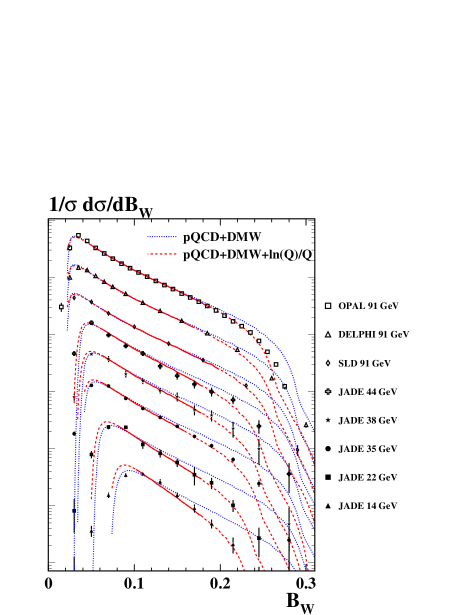
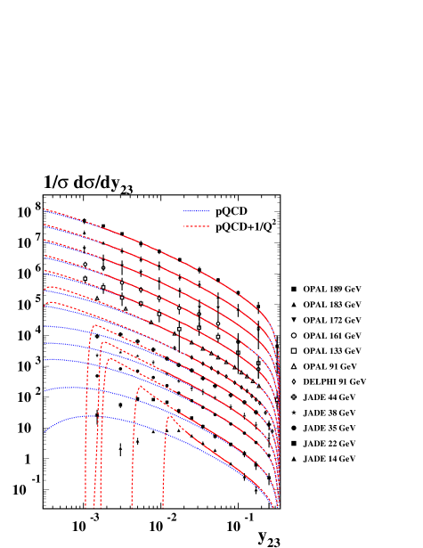
Figure 5 (left) shows results of simultaneous fits of $\alpha_{\mathrm{S}}(m_{\mathrm{Z^{0}}})$ and $\alpha_{0}(2~{}\mathrm{GeV})$ to data for distributions of $B_{W}$ at $14\leq\sqrt{s}\leq 91$ GeV pedrophd . The solid lines indicate results of extended fits where an additional term $A_{11}\ln(Q)/Q$, $Q=\sqrt{s}$, with a new free parameter $A_{11}$ has been added to the DMW prediction. The fit describes the data well and yields $\chi^{2}/\mathrm{d.o.f.}=22/23$. The same fit without the additional term is shown by the dotted lines; the fit does not describe the data at low $\sqrt{s}$ well and $\chi^{2}/\mathrm{d.o.f.}=66/24$ is found. One thus has evidence for additional contributions to this observables at low $\sqrt{s}$ probably behaving like $\ln(Q)/Q$.

Figure 5 (right) shows results of simultaneous fits of $\alpha_{\mathrm{S}}(m_{\mathrm{Z^{0}}})$ and $\alpha_{0}(2~{}\mathrm{GeV})$ to data for distributions of $y_{23}^{\mathrm{D}}$ at $14\leq\sqrt{s}\leq 189$ GeV. The solid lines show fits of the pure perturbative QCD prediction with an additional term of the form $A_{20}/Q^{2}$ inspired by dokshitzer95a . The fit describes the data at all cms energies and $\chi^{2}/\mathrm{d.o.f.}=71/106$ is found. The dotted lines present the results of the same fits without the additional power correction term. The fit does not describe well the data at low cms energies, in particular at $\sqrt{s}=14$ and 22 GeV. One thus has evidence for additional terms probably behaving like $1/Q^{2}$ at low $\sqrt{s}$. At large cms energies the two types of fit are very similar.

Figure 5: (left) Distributions of $B_{W}$ measured at $14\leq\sqrt{s}\leq 91$ GeV as shown on the figure pedrophd . Superimposed are fits perturbative QCD combined with power corrections with (solid and dashed lines) and without (dotted lines) additional terms as explained in the text. (right) Distributions of $y_{23}^{\mathrm{D}}$ measured at $14\leq\sqrt{s}\leq 189$ GeV as shown on the figure pedrophd . Superimposed are fits of pure perturbative QCD (solid and dashed lines) or perturbative QCD combined with a power correction term as explained in the text.

IV EVIDENCE FOR SOFT FREEZING

One of the main assumptions of the DMW model of power corrections is, simply speaking, that the physical running strong coupling $\alpha_{\mathrm{S}}^{\mathrm{NP}}$ remains finite around and below the Landau pole, where the perturbative evolution of the strong coupling according to the renormalisation group brakes down. With this assumption quantities like $\alpha_{0}(\mu_{\mathrm{I}})=1/\mu_{\mathrm{I}}\int_{0}^{\mu_{\mathrm{I}}}\alpha_{\mathrm{S}}^{\mathrm{NP}}(k)\mathrm{d}k$ can be defined.

Using hadronic decays of $\tau$ leptons this question can be studied experimentally. The $\tau$ lepton decays weakly via an intermediate (virtual) $\mathrm{W^{+}}$ or $\mathrm{W^{-}}$ boson. When the W boson decays to quarks QCD effects have to be taken into account. The mass of the virtual W bosons $m_{\mathrm{W}}\leq m_{\tau}=1.777$ GeV sets the scale for these effects which are rather large. The spectrum of invariant masses of hadronic final states from $\tau$ lepton decays provides a direct experimental measurement of the scale given by the virtual $m_{\mathrm{W}}$.

Figure 6 left shows a measurement of the inclusive spectrum of invariant masses of non-strange hadronic final states $s=m_{h}^{2}$ by OPAL OPALPR246 . The quantity $v(s)+a(s)=\mathrm{d}R_{\tau}/\mathrm{d}s$ with $R_{\tau}(s)=\Gamma(\tau\rightarrow\mathrm{h}\nu_{\tau})/\Gamma(\tau\rightarrow\ell\nu_{\ell}\nu_{\tau})$. The dashed line shows the “parton model prediction” for three colours. The solid line shows the perturbative QCD prediction for massless quarks. The line describes the correlated data points well; this implies that non-perturbative corrections are small for the inclusive spectrum.

Figure 6: (left) Spectrum of invariant masses of $\tau$ lepton decays into non-strange hadronic final states OPALPR246 . The solid and the dashed line show predictions as indicated on the figure. (right) The effective charge $\alpha_{\tau}$ determined from hadronic $\tau$ decays as explained in the text as a function of $s$ brodsky03 . The lines show varios predictions for $\alpha_{\tau}(s)$ as explained in the text.

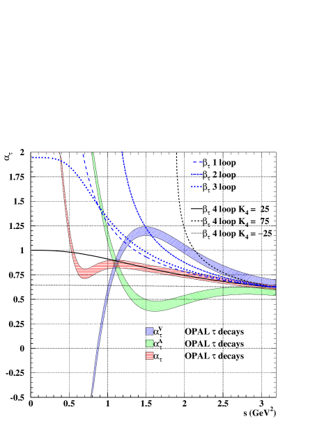The analysis brodsky03 defines an effective charge $\alpha_{\tau}(s)$ via $R_{\tau}(s)=R_{\tau}^{0}(1+\alpha_{\tau}(s)/\pi)$. The relation between $\alpha_{\tau}(s)$ and $\alpha_{\mathrm{S}}(s)$ is known perturbatively. Figure 6 (right) shows the variable $\alpha_{\tau}(s)$ as a function of $s$ extracted from the data (shaded bands) and using different predictions (lines). The band from analysis of the inclusive spectrum labelled “$\alpha_{\tau}$” stays fairly flat down to $s\simeq 1$ GeV² and then rises steeply due to the $\rho$ resonance. The other bands are from analysis of spectra for even or odd number of pions in the final state and have strong non-perturbative effects. The solid line labelled “$\beta_{\tau}$ 4 loop $K_{4}=25$” corresponds to the most complete QCD prediction for the running of the effective charge including an estimate of 4th order term. This prediction describes the data well down to $s\simeq 1$ GeV² and stays finite at $s=0$. One also observes that the NNLO prediction labelled “$\beta_{\tau}$ 3 loop” also describes the data at medium values of $s$ and is finite at $s=0$. It is thus possible to consistently describe data for hadronic $\tau$ decays down to $s\simeq 1$ GeV² with an effective coupling which stays finite at $s=0$. These observations are consistent with earlier work howe02 ; howe03 .

V SUMMARY AND OUTLOOK

In this review several topics were not covered due to a lack of results. One issue is the study of 4-jet event shape observables in the planar limit. The theoretical aspects and preliminary experimental results are discussed in contributions B001 and B002 to this conference. However, there are no published experimental studies which could be subject of this review, but hopefully there will be results on this important subject in the near future. Other models for the description of soft corrections to hard QCD processes such as shape functions, the single-dressed-gluon approximation (SDG) are subject of contributions to this conference but there are no detailed experimental studies. From an experimental point of view the DMW model is attractive, because it makes strong predictions about relations between observables and has only universal free parameters. Also, predictions actually exist for several observables such that direct comparisons are possible.

The power corrections in the DMW model have been studied by several experimental groups as presented in this review. The picture is generally consistent with only a few notes:

• The values for $\alpha_{0}(2~{}\mathrm{GeV})$ from different observables are consistent within 20 to 30%. However, it has to be understood if this is a variation one expects from the theoretical uncertainties in the calculations. It is often claimed that the theoretical uncertainty on the Milan factor $M$ of about 20% due to missing higher order terms could explain the scatter of $\alpha_{0}(2~{}\mathrm{GeV})$ results. However, since $M$ is a universal factor it is not clear if it can explain differences between different observables.

• The values for $\alpha_{\mathrm{S}}(m_{\mathrm{Z^{0}}})$ from different observables are consistent with each other within the uncertainties of the perturbative QCD calculations as expected. However, direct comparison of the results from power correction analyses and analyses with hadronisation corrections derived from Monte Carlo simulation show a systematic bias for $\alpha_{\mathrm{S}}(m_{\mathrm{Z^{0}}})$ of about 6% (mean values) or 9% (distributions). This bias is comparable to or larger than the total uncertainties quoted for determinations of $\alpha_{\mathrm{S}}(m_{\mathrm{Z^{0}}})$ from event shape or jet observables in $\mathrm{e^{+}e^{-}}$ annihilation. The bias is significantly larger than the hadronisation model uncertainties of less than 2% quoted for $\alpha_{\mathrm{S}}(m_{\mathrm{Z^{0}}})$ determinations using LEP data kluth06 .

In the future the studies of power corrections with $\mathrm{e^{+}e^{-}}$ annihilation data would profit from further analyses using the JADE data in the intermediate energy region $14\leq\sqrt{s}\leq 44$ GeV. In particular the EEC and 4-jet observables with or without requiring the planar limit would be attractive subjects.

The impact of NNLO perturbative QCD calculations for 3-jet observables could also be significant. Firstly, the power correction calculations will have to adapted to the improved predictions. Secondly, with there is potential for high precision measurements of $\alpha_{\mathrm{S}}(m_{\mathrm{Z^{0}}})$ with reduced theoretical uncertainties. With selected observables with suppressed power corrections such as $y_{23}^{\mathrm{D}}$ one could obtain the matching reduced hadronisation uncertainties.

Other approaches to understand soft corrections in terms of QCD should be studied in more detail. The connection with RS optimisation discussed in contributions T001 and T002 is also an interesting new area of research.

References

- (1) S. Kluth: Rept. Prog. Phys. 69 (2006) 1771
- (2) M. Dasgupta, G.P. Salam: J. Phys. G 30 (2004) R143
- (3) S. Kluth: In: 2001 QCD and High Energy Hadronic Interactions, J.TrânThanh Vân (ed.), 115. The Gioi Publishers, Vietnam, 2002, Contributed to XXXVIth Recontre de Moriond, QCD and High Energy Hadronic Interactions, Les Arcs, France, March 17–24, 2001
- (4) S. Kluth: Nucl. Phys. Proc. Suppl. 109B (2002) 87
- (5) B. Naroska: Phys. Rep. 148 (1987) 67
- (6) D. Degele: In: 11th international conference on high energy accelerators, W.S. Newman (ed.), Vol. 40 of Experientia Supplementum, 16. Birkhäuser Verlag, 1980
- (7) S. Bethke: MPI-PhE/2000-02 (2000), hep-ex/0001023
- (8) JADE and OPAL Coll., P. Pfeifenschneider et al.: Eur. Phys. J. C 17 (2000) 19
- (9) L3 Coll., P. Achard et al.: Phys. Rep. 399 (2004) 71
- (10) OPAL Coll., G. Abbiendi et al.: Eur. Phys. J. C 40 (2005) 287
- (11) ALEPH Coll., A. Heister et al.: Eur. Phys. J. C 35 (2004) 457
- (12) DELPHI Coll., J. Abdallah et al.: Eur. Phys. J. C 37 (2004) 1
- (13) S. Kluth et al.: Eur. Phys. J. C 21 (2001) 199
- (14) Yu.L. Dokshitzer, G. Marchesini, B.R. Webber: Nucl. Phys. B 469 (1996) 93
- (15) B.R. Webber: Phys. Lett. B 339 (1994) 148
- (16) Yu.L. Dokshitzer, B.R. Webber: Phys. Lett. B 352 (1995) 451
- (17) S.J. Brodsky, S. Menke, C. Merino, J. Rathsman: Phys. Rev. D 67 (2003) 055008
- (18) Yu.L. Dokshitzer, B.R. Webber: Phys. Lett. B 404 (1997) 321
- (19) Yu.L. Dokshitzer, A. Lucenti, G. Marchesini, G.P. Salam: J. High Energy Phys. 5 (1998) 003
- (20) Yu.L. Dokshitzer, G. Marchesini, G.P. Salam: Eur. Phys. J. direct C 3 (1999) 1
- (21) DELPHI Coll., J. Abdallah et al.: Eur. Phys. J. C 29 (2003) 285
- (22) Y.L. Dokshitzer, G. Marchesini, B.R. Webber: JHEP 07 (1999) 012
- (23) P.A. Movilla Fernández, S. Bethke, O. Biebel, S. Kluth: Eur. Phys. J. C 22 (2001) 1
- (24) G.P. Salam, D. Wicke: J. High Energy Phys. 05 (2001) 061
- (25) P.A. Movilla Fernández: Ph.D. thesis, RWTH Aachen, 2003, PITHA 03/01
- (26) OPAL Coll., K. Ackerstaff et al.: Eur. Phys. J. C 7 (1999) 571
- (27) D.M. Howe, C.J. Maxwell: Phys. Lett. B 541 (2002) 129
- (28) D.M. Howe, C.J. Maxwell: Phys. Rev. D 70 (2004) 014002