Effective Charges in Practice

Abstract

Experimental results on event shapes obtained within (or related to) the method of Effective Charges are discussed in view of measurements of the strong coupling, $\alpha_{s}$, the $\beta$-function and non-perturbative contributions to event shapes. The data strongly advocate to use of the ECH scheme instead of the conventional $\overline{\text{MS}}$ scheme.

I Introductory Remarks

I.1 Assorted Theoretical Formulae and Results

Today the $\overline{\text{MS}}$-scheme is the de facto standard used for comparisons of QCD predictions as well as experimental results. It was introduced for practical reason, as an offspring of dimensional regularisation, whereas the method of Effective Charges (ECH) and the corresponding renormalisation scheme are motivated physically. The ECH method has been in some detail discussed in the talk of Maxwell maxtalk . For completeness here the basic formulae and results are assembled in view of the later interpretation of the data.

ECH has been originally introduced in Grunberg:1982fw , a clear access, taking the observable itself as perturbative expansion parameter (called renormalisation group improved perturbation theory, RGI) is given in Dhar:1983py . With respect to ECH I follow the arguments of Barclay:1994qa which applies the ECH method directly to $\text{e}^{+}\text{e}^{-}$data. The results especially apply to mean values (or moments) of the event shape distributions which depend on a single energy scale, the centre-of-mass energy, $Q=\sqrt{s}$, only.

The general next-to-leading order (NLO) expression for event shape distributions of an observable $y$ reads:

$$\frac{1}{\sigma_{tot}}\frac{d\sigma(y)}{dy}=\frac{\alpha_{s}(\mu^{2})}{2\pi}\cdot A(y)+\left(\frac{\alpha_{s}(\mu^{2})}{2\pi}\right)^{2}\cdot\left[B(y)+\frac{1}{2}\beta_{0}\ln(x_{\mu})\cdot A(y)\right]+{\cal{O}}(\alpha_{s})^{3}$$ (1)

Here $A$ and $B$ are the first and second order coefficients of the perturbative expansion. Note that due to the normalisation to the total cross-section the integral of Eqn. 1 is normalised to 1. The $\mu^{2}$ (or alternatively the $x_{\mu}=\mu^{2}/Q^{2}$) dependence reflects the dependence of the prediction on the renormalisation scheme. In NLO the change of renormalisation scheme is fully equivalent to the change of the renormalisation scale.

Weighting Eqn. 1 with and integrating over the observable then yields the mean value $\langle y\rangle$ which can be directly measured. Normalising $\langle y\rangle$ to the leading order coefficient $A$ a measurable quantity $R$ is obtained. Such quantities are called effective charges. The idea of the ECH method is now to chose (in any order of perturbation theory) a scheme such that all higher order coefficients for $R$ vanish. This implies that $R$ coincides with the strong coupling extracted in a leading order analysis and explains the name ECH as such observables are directly comparable to other observables of this kind as well as to the coupling. In NLO this leads to the following scale:

$$\mu_{\text{ECH}}=Q\cdot e^{-\frac{1}{\beta_{0}}\frac{B(y)}{A(y)}}$$ (2)

An effective charge $R$ obeys the Renormalisation Group Equation (RGE):

$$\frac{dR}{d\ln Q^{2}}=\beta_{R}(Q)\quad=\quad-\frac{\beta_{0}}{4}R^{2}\cdot\left[1+\rho_{1}R+\rho_{2}R^{2}+\dots\right]\quad+\quad K_{0}\cdot e^{-S/R}R^{\delta}+\dots$$ (3)

As the observables $R$ are directly measurable in dependence of the energy the $\beta_{R}$-functions are measurable quantities. The leading coefficients of the $\beta$-functions, $\beta_{0}=11-2/3\cdot n_{f}$ and $\rho_{1}=\beta_{1}/2\beta_{0}$ are universal (the same as for the coupling), the higher coefficients are observable dependent but free of renormalisation scheme ambiguities. Non-perturbative contributions, invisible in perturbation theory, lead to the term with the exponential. $K_{0}$ is proportional to the factor multiplying a power term in the usual power model expressions. Omitting for simplicity the non-perturbative term Eqn. 3 can be integrated yielding:

$$\frac{\beta_{0}}{2}\ln\frac{Q}{\Lambda_{R}}=\frac{1}{R}+\rho_{1}\ln\frac{\rho_{1}R}{1+\rho_{1}R}+\int_{0}^{R}\left\{-\frac{1}{\rho(x)}+\frac{1}{x^{2}(1+\rho_{1}x)}\right\}dx\quad,$$ (4)

where $\rho(R)$ is defined by the square bracketed term in Eqn. 3. The constant of integration, $\Lambda_{R}$, should have physical significance and is related to $\Lambda_{\overline{\text{MS}}}$ by an exact expression Celmaster:1979km . Thus $\alpha_{s}(M_{\text{Z}})$ can be calculated from $\Lambda_{R}$ practically without additional uncertainty.

Besides the derivation of the above fundamental equations the paper Barclay:1994qa includes a broad discussion of the extraction of $\Lambda_{\overline{\text{MS}}}$ from $\text{e}^{+}\text{e}^{-}$data and shows the following:

• The ECH formalism … is more general than the adoption of a particular scheme … It can be derived non-perturbatively assuming only that the high energy behavior of the observable is given by the leading order perturbative expression.

• … higher orders can be split into a predictable contribution (of known “RG predictable” terms $\propto\log{\mu/Q}$) and a remaining piece containing all the genuinely unknown aspects. … the choice $\mu=\mu_{\text{ECH}}$ removes the predictable scatter and provides genuine information on the interesting … higher-order terms.

• One can exhibit the relative size of the (truly) uncalculated higher-order corrections for different quantities. These corrections are related to how the energy dependence of the quantity differs from its asymptotic dependence as $Q^{2}\to\infty$.

• … by comparing with data one can test how well the first few perturbative terms represent the observed running. Marked discrepancies indicate the importance of higher order terms, or … non-perturbative contributions.

These findings imply that the ECH scheme offers exceptional experimental control of higher order contributions by comparing different effective charge observables or measuring their energy evolution.

I.2 Remarks on Experimental Data

The later discussion is mainly based on precise data of shape distributions obtained at the Z-peak and of their mean values in the full range of $\text{e}^{+}\text{e}^{-}$ experiments above the b-threshold. Some more recent results Abdallah:2003xz ; ralle ; Pfeifenschneider:1999rz ; MovillaFernandez:1997fr refer to the energy range $\sim$20-202GeV and comprise data on events with a radiated hard photon ($45{\mbox{Ge\kern-0.86108ptV}}<\sqrt{s\textasciiacute}<M_{Z}$) Abdallah:2003xz ; ralle . All experimental results correspond to simple $\text{e}^{+}\text{e}^{-}$ annihilation and are fully corrected for experimental effects.

It has been realised Salam:2001bd , that hadron mass effects have a particularly strong influence for the so-called jet mass observables. This strong mass dependence has been avoided in Abdallah:2003xz ; ralle by redefining the particle four momenta using the so called p-scheme: ($(\vec{p},E)\to(\vec{p},|\vec{p}|)$) or E-scheme: ($(\vec{p},E)\to(\hat{p}E,E)$). Moreover in Abdallah:2003xz ; ralle extra transverse momentum from B-hadron decays was corrected for by using Monte Carlo. This correction is power behaved and can have influence on the energy evolution of the observables. A figure displaying the correction is included in Abdallah:2003xz .

B-decays also influence event shape distributions. For 2-jet like topologies the distributions are depleted. These events are shifted towards 3-jet topologies by the extra transverse momentum from the decay. For observables calculated from the whole event (like $B_{T}$) the decay from the narrow event side contributes for all values of the observable leading to visible effects in the whole range of the observable. In principle, the differences between the observables due to B-decays need to be corrected when applying power correction models to shape distributions. Plots of such corrections are again included in Abdallah:2003xz ; ralle .

II Results on Event Shape Distributions

II.1 Effects of Changing the Renormalisation Scale

Figure 1: ${\cal{O}}(\alpha_{s}^{2})$ prediction for $\tau=1-\text{Thrust}$ for $x_{\mu}$=1 and for the experimentally optimised value of $x_{\mu}$.

Figure 2: $\alpha_{s}(M_{\text{Z}})$ from $\tau=1-\text{Thrust}$ as function of $\tau$ for $x_{\mu}$=1 and for the experimentally optimised value of $x_{\mu}$.

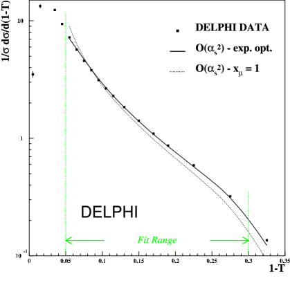
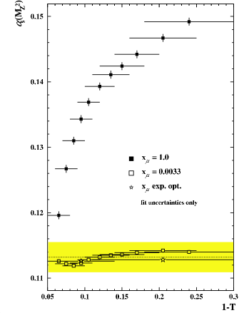
Analyses of event shape distributions performed by experimental collaborations mainly employed the $\overline{\text{MS}}$-scheme with $x_{\mu}=1$; information about the explicit use of the ECH scheme Abreu:2000ck ; siggi ; Burrows:1995vt is sparse. Several experiments attempted, however, to determine optimal scales by fitting $\alpha_{s}$ and $x_{\mu}$ simultaneously to the data. In view of this, so called experimental optimisation, it is instructive to discuss the influence of $x_{\mu}$ on the prediction Eqn. 1. In Fig. 2 the data on $\tau=1-\text{Thrust}$ is compared with the prediction Eqn. 1 for $x_{\mu}=1$ and the optimised scale ($x_{\mu}\sim 0.0033$). Evidently the change of scale leads to a “turn” of the prediction. For $x_{\mu}=1$ the slope of the data is barely described. Other observables show a similar though often less pronounced discrepancy. As a consequence the quality of the fits for $x_{\mu}$=1 is, in general, unsatisfactorily bad and the fitted values of $\alpha_{s}$ depend on the interval chosen for the fit. This is shown in Fig. 2 e.g. for the Thrust siggi .

This behavior is basically known since Petra Magnussen:1989eh or the early days of Lep and has been observed at small values of the event shape observables (in the 2-jet region) where the perturbative ${\cal{O}}(\alpha_{s}^{2})$ predictions are presumed little reliable. It should be noted, however, that due to the normalisation of the event shape distributions $1/\sigma\int d\sigma/dy~{}dy=1$, the misfit between data and prediction must persist at large $y$ if present at small $y$. This has indeed been seen Abreu:2000ck ; siggi .

The optimisation of a single scale value for a distribution has been criticised Barclay:1994qa as, in principle, the scale is expected to be $y$-dependent (compare Eqn. 2). However, the change of scale expected in the typical fit ranges of the data is moderate (compare Fig. 6). Experimental optimisation therefore presents a fair compromise between theoretical prejudice or request and experimental feasibility.

Results on experimental optimisation are included in Abreu:2000ck ; Burrows:1995vt ; Abreu:1992yc ; Acton:1992fa . The first reference, which is discussed below, comprises 18 observables and is based on high statistics data. Moreover in this analysis the dependence of the event shape distributions on the polar angle of the event axis with respect to the beam has been exploited. This is advantageous in view of experimental systematics and leads to a large number of statistically independent data points.

Consequences for Matched NLLA ${\cal{O}}(\alpha_{s}^{2})$ Analyses
The mismatch of the slope of data and ${\cal{O}}(\alpha_{s}^{2})$ prediction has consequences also for the analysis of event shape distributions with matched NLLA/${\cal{O}}(\alpha_{s}^{2})$ predictions.

Figure 3: Ratio data over NLLA/${\cal{O}}(\alpha_{s}^{2})$-fit from Opal Abbiendi:2004qz ; Ford:2004dp (lines added by the author).

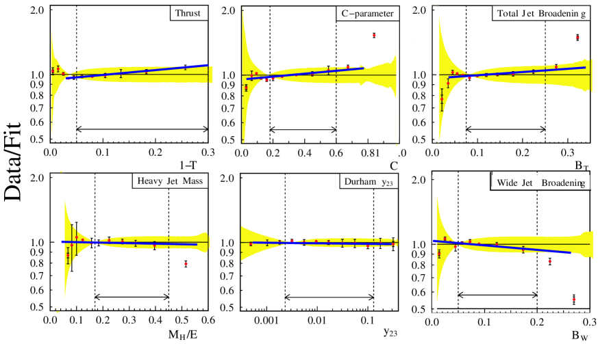
The matching from an experimental point of view represents a kind of “averaging” of both predictions where in the 2-jet regime the NLLA part and in the 3-jet regime the ${\cal{O}}(\alpha_{s}^{2})$ part dominates. As in the matching the ${\cal{O}}(\alpha_{s}^{2})$ prediction is used with a renormalisation scale value $x_{\mu}$=1 the slope of the data is, for many observables, imperfectly described. In consequences the same problems as discussed above for the pure ${\cal{O}}(\alpha_{s}^{2})$ prediction persist, though diminished by the matching with the NLLA part. In consequence the $\chi^{2}/N_{df}$ is often in-acceptably bad when applying standard rules. Additional theory errors are introduced to regain consistency. As in the ${\cal{O}}(\alpha_{s}^{2})$ case the fitted value of $\alpha_{s}(M_{\text{Z}})$ often shows a marked dependence on the observable. To illustrate this in Fig. 3 the ratio of the data and the fitted matched predictions is shown for several observables from the concluding Opal analysis on event shape distributions Abbiendi:2004qz ; Ford:2004dp . In order to make the discrepancies directly visible straight lines are additionally put to the data points. For $T$, $C$ and $B_{T}$ a clear increase of the ratio with increasing values of the observables is seen corresponding to an increase of $\alpha_{s}$ ($\gtrsim 5\%$). For $M_{H}/E$ and $y_{23}$ the ratio is almost constant, while for $B_{W}$ the ratio decreases with increasing observable. This more complicated pattern correlates with the importance of higher order corrections in the ${\cal{O}}(\alpha_{s}^{2})$ part of the prediction or simply with the ratio $B/A$. The three observables with increasing ratio also show a large ratio $B/A>15$, for $M_{H}/E$ and $y_{23}$ the ratio is smaller. For $\langle B_{W}\rangle$ it is negative. The mismatch of the slope of the data and the prediction also deteriorates the initial $\chi^{2}/N_{df}$. The constructed error bands (dominated by “theory errors”) restore consistency of the fits. The best stability is obtained for $y_{23}$ and justifies the small error obtained for this observable (see Fig. 3 and Abbiendi:2004qz ; Ford:2004dp ; Heister:2002tq ).

Still the $\alpha_{s}(M_{\text{Z}})$ values depend on the fit range for some observables and are thus biased. This observable dependent biases is even present in the overall Lep combination (see Fig. 10, QCDwg ). The (correlated) $\alpha_{s}$ values from $T$ and $B_{T}$ are high, $y_{23}$ and $B_{W}$ are low compared to the average. $C$ is close to the average and seems to form an exception.

It is likely that the imperfect description of the slope by the matched prescription similarly influences analyses of power terms introduced in order to describe the hadronisation. E.g. in the corresponding Delphi analysis Abdallah:2003xz the $\alpha_{s}$ values for $B_{T}$ and $\rho_{h}=M^{2}_{h}/s$ (E-scheme) are markedly smaller compared to the results from $B_{W}$, $T$ and $\rho_{s}$.

II.2 Results from Distributions on Experimentally Optimised Scales

Figure 4: $\Delta\chi^{2}$ and $\alpha_{s}(M_{\text{Z}})$ obtained from ${\cal{O}}(\alpha_{s}^{2})$ fits of 18 event shape distributions as function of $x_{\mu}$ siggi .

Figure 5: $\alpha_{s}(M_{\text{Z}})$ results obtained from ${\cal{O}}(\alpha_{s}^{2})$ fits of 18 event shape distributions for $x_{\mu}$=1 and $x_{\mu}$=$x_{\mu}^{\text{opt}}$.

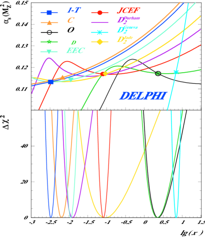
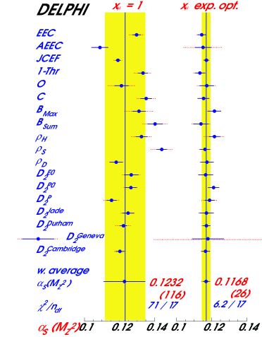
In Fig. 5 the $\Delta\chi^{2}$ and $\alpha_{s}(M_{\text{Z}})$ as function of $x_{\mu}$ as obtained from several event shape distributions is shown Abreu:2000ck ; siggi . The fit quality for these fits is satisfactory when including experimental and hadronisation errors only. Marked minima in $\Delta\chi^{2}$ are observed scattered over a wide range of $x_{\mu}$. The clear minima imply that the optimised scale values are statistically well determined. The $\alpha_{s}(M_{\text{Z}})$ results corresponding to these scales show a much smaller scatter as for fixed $x_{\mu}$=1. This is more clearly shown in Fig. 5. The spread reduces from $9.4\%$ for $x_{\mu}$=1 to 2.2% with optimised scales, $x_{\mu}^{\text{opt}}$.

Figure 6: Correlation of the experimentally optimised scale $x_{\mu}^{\text{opt}}$ values with the ECH expectation $x_{\mu}^{ECH}$. The errors of $x_{\mu}^{\text{opt}}$ are fit errors, for $x_{\mu}^{ECH}$ they indicate the expected change in the fit range.

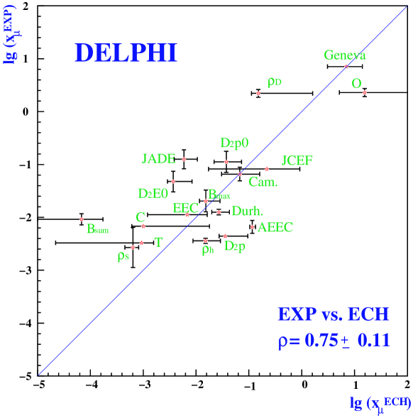
It is particularly interesting to study the correlation of the fitted $x_{\mu}^{\text{opt}}$ with the values expected from ECH, $x_{\mu}^{\text{ECH}}$, shown in Fig. 6. The $x_{\mu}^{\text{opt}}$-errors are from the fit, the error bars for $x_{\mu}^{\text{ECH}}$ indicate the range of scales expected within the fit interval of the data. A significant correlation $\rho=0.75\pm 0.11$ is observed. The wide spread of experimentally optimised scales which has been often criticised is in fact slightly smaller than the range expected from ECH.

Regarding the distribution of individual observables (indicated by the letters in the plot) it is seen that observables calculated from the whole event (e.g. the Thrust) tend to populate the region of small $x_{\mu}^{\text{ECH}}$, observables sensitive mainly to the wide side of the events (e.g. $\rho_{h}$) populate the center while observables from the difference of the wide and narrow side show large scales. This ordering corresponds (via Eqn. 2) to large (for small $x_{\mu}^{\text{ECH}}$) and small second order $\overline{\text{MS}}$ contributions (for big $x_{\mu}^{\text{ECH}}$). Overall the observed large range of $x_{\mu}^{\text{opt}}$ can be considered as understood in ECH theory.

It may be worth noting that the RMS spread of $x_{\mu}^{\text{opt}}$ with respect to $x_{\mu}^{\text{ECH}}$ is only 2.5 (i.e. similar to the range used for naive $\overline{\text{MS}}$ theory error estimates). This may be taken as a justification of an ECH theory error estimate by a corresponding scale change. However, the corresponding $\alpha_{s}$ uncertainty will be far smaller than in the $\overline{\text{MS}}$ case as the optimal scales often correspond to the minima of the $\alpha_{s}(M_{\text{Z}})$($x_{\mu}$) curves (compare Fig. 5).

II.3 Results from Event Shape Mean Values

Figure 7: RGI fits to several event shape means as function of the centre-of-mass energy (full line). The dashed line represents the $\overline{\text{MS}}$-expectation (with the same $\alpha_{s}(M_{\text{Z}})$).

Figure 8: $\alpha_{s}(M_{\text{Z}})$ results obtained from several event shape means or integrals over the JCEF or EEC using $\overline{\text{MS}}$ theory plus Monte Carlo or power hadronisation corrections and RGI theory with and without non-perturbative terms.

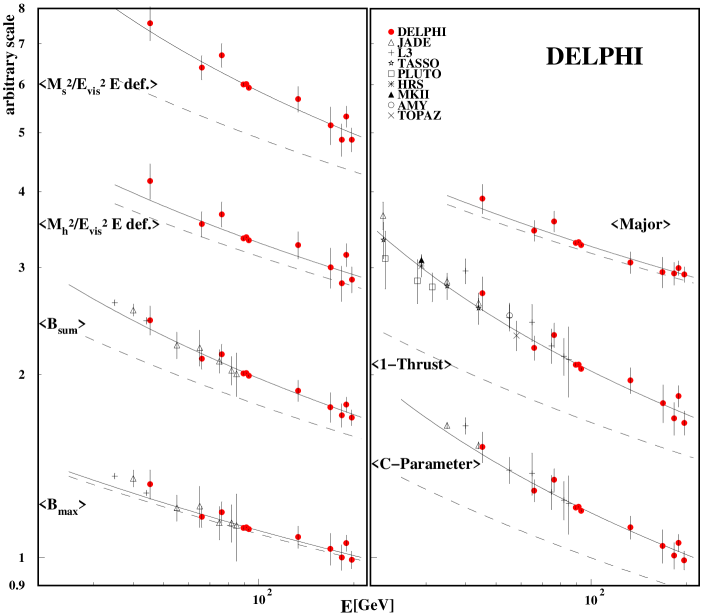
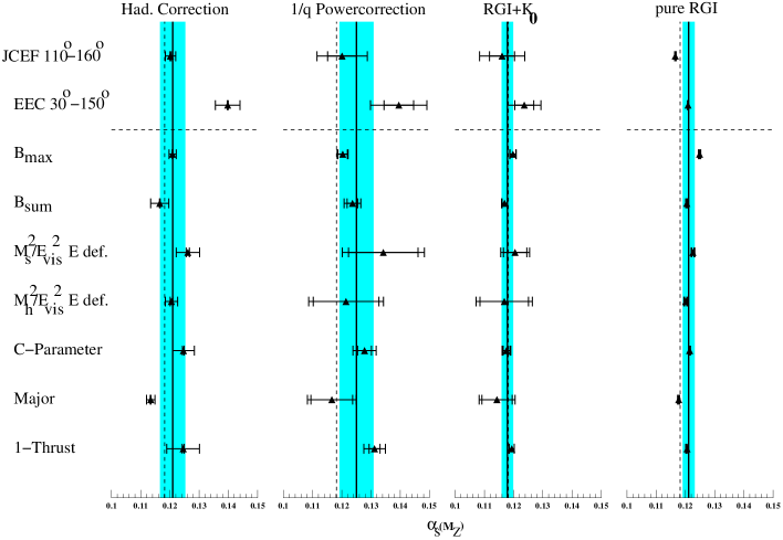
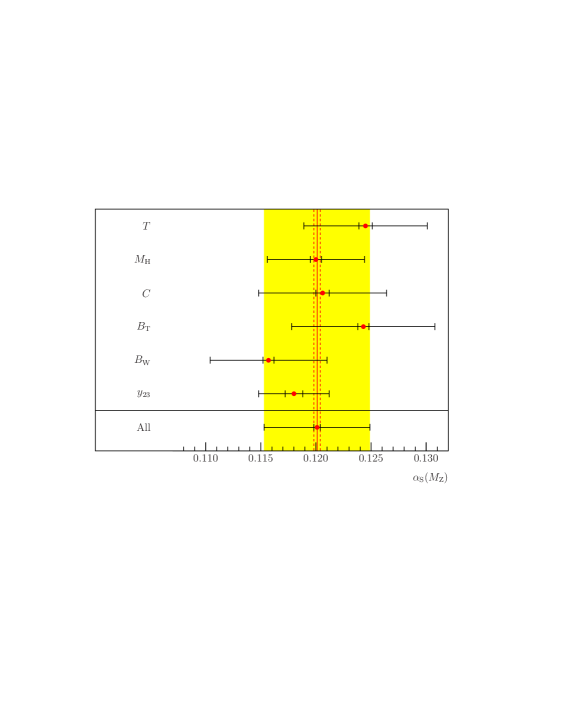
Some relevant data on mean values of shape distributions as function of the centre-of-mass energy Abdallah:2003xz is shown in Fig. 8. The data is compared to fits of Eqn. 4 shown as full lines. The dashed lines represent the $\overline{\text{MS}}$-prediction for the same $\alpha_{s}(M_{\text{Z}})$. It turned out that the data can be well described by the ECH/RGI fits with a single value of $\alpha_{s}(M_{\text{Z}})$ ($\sim 0.120$) and negligible additional non-perturbative terms. In Fig. 8 the $\alpha_{s}(M_{\text{Z}})$ results obtained from this data with $\overline{\text{MS}}$ prediction and Monte Carlo or power hadronisation corrections and ECH/RGI theory with and without power terms are compared. Evidently the spread of the results is far smaller for the ECH/RGI results. The inclusion of power terms leaves the spread almost unchanged but lowers the average value of $\alpha_{s}(M_{\text{Z}})$ to $0.118$. This result implies that the differences due to non-trivial uncalculated higher order terms or non-perturbative terms is small, of ${\cal{O}}(2\%)$. Note that higher order corrections differing by about a factor 2 (in $\overline{\text{MS}}$) are expected  for event shape observables calculated from the full event or the wide hemisphere of an event only. This is also reflected e.g. in the perturbatively calculated ratio of the power terms of Thrust and $\rho_{h}$. The bigger differences seen in the $\overline{\text{MS}}$ compared to the ECH results then should be due to “RG predictable” $\log\mu/Q$ terms.

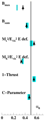
The better agreement of the ECH result is also illustrated by Fig. 10 where the measured size of the power terms for some observables as parameterised by $\alpha_{0}$ is compared to the ECH/RGI expectation which has been calculated by setting the $\overline{\text{MS}}$+power terms expression equal to the ECH prediction. It is evident that the RGI/ECH prediction describes the data better than a universal value of $\alpha_{0}$ presumed by power correction models.

Figure 9: Combined Lep $\alpha_{s}(M_{\text{Z}})$ results for different observables Ford:2004dp .

Figure 10: Size of the non-perturbative terms $\alpha_{0}$ as determined from power model fits compared to ECH expectation (grey bands).

Table 1: Results on $\beta_{0}$ obtained from RGI/ECH fits to Delphi data Abdallah:2003xz . The first error is statistical, the second is systematic and the third is due to the B-hadron decay correction. The uncertainty due to possible non-pert. contributions is small.

Observable	$\mathbf{\beta_{0}}$	$\mathbf{\chi^{2}/N_{df}}$
$\langle 1-\text{Thrust}\rangle$	$7.7\pm 1.1\pm 0.2\pm 0.1$	$9.2/13$
$\langle\text{C-parameter}\rangle$	$7.8\pm 1.0\pm 0.3\pm 0.1$	$7.2/13$
$\langle\rho_{h}\rangle$ E-def.	$7.5\pm 1.5\pm 0.2\pm 0.0$	$8.8/13$
$\langle\rho_{s}\rangle$ E-def.	$7.5\pm 1.1\pm 0.2\pm 0.0$	$7.1/13$
$\langle B_{\text{W}}\rangle$	$7.7\pm 1.4\pm 0.1\pm 0.1$	$6.3/13$
$\langle B_{\text{T}}\rangle$	$7.7\pm 0.9\pm 0.1\pm 0.1$	$5.9/13$
$\langle{\text{Major}}\rangle$	$8.0\pm 1.1\pm 0.1\pm 0.1$	$9.2/13$

Besides the comparison of the $\alpha_{s}$ results from different observables the energy dependence of these observables i.e. the observed $\beta_{R}$-functions can be compared to the NLO expectation. As the NLO terms present only a small ${\cal{O}}(4\%)$ correction $\rho_{1}$ has been set to the QCD expectation. Then the $\beta_{0}$ values obtained from the different observables can be directly compared. In order to allow full control of the systematic uncertainties this comparison was made for seven observables determined from Delphi data only. The measured $\beta_{0}$ values agree among each other within part of the correlated statistical uncertainty and with the QCD expectation $\beta_{0}=7.66$ (see Tab. 1). The possible influence of power terms ($\sim 2\%$ at the Z) on the $\beta$-function is small as the energy dependencies of the power terms and the $\beta$-function are similar.

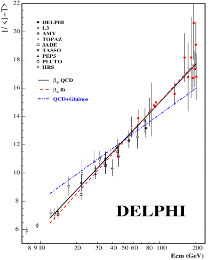
Especially in view of a measurement of the $\beta$-function the analysis has been repeated including reliable low energy data on the Thrust. The resulting fit is shown in Fig. 12, and corresponds to

$$\beta_{0} =7.86\pm 0.32\quad.$$ (5)

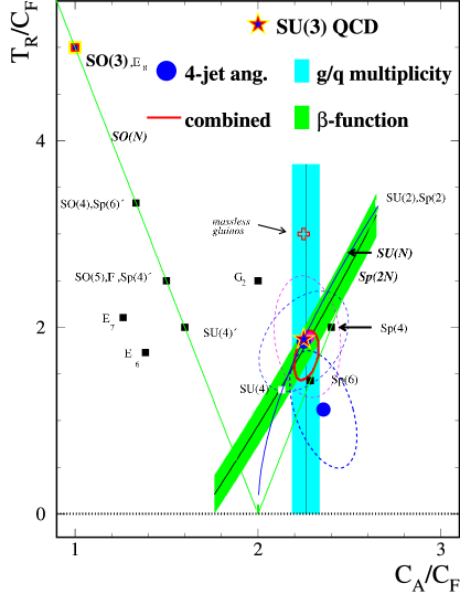
This measurement of the $\beta$-function is the most precise presented so far and allows to strongly constrain the QCD gauge group to SU(3) in combination with measurements of the multiplicity ratio of gluon and quark jets Abdallah:2005cy and four jet angular distributions Heister:2002tq ; Abreu:1997mn ; Abbiendi:2001qn (see Fig. 12). This agreement in turn lends further support to the measurements using the ECH scheme.

Figure 11: ECH/RGI fit to data on $\langle 1-\text{Thrust}\rangle$. The data is corrected for the small influence of B-hadron decays. The full line represents the QCD expectation, the dashed-dotted line the expectation for QCD plus light Gluinos.

Figure 12: Constraints on $C_{A}/C_{F}$ and $T_{R}/C_{F}$ from measurements of the $\beta$-function, the multiplicity ratio in gluon to quark jets and four jet angular distributions.

As a final check it has been tried to infer the possible size of $\rho_{2}$ from the overall Thrust data by fitting the corresponding expression with $\beta_{0}$ and $\rho_{1}$ fixed to the QCD expectation. The resulting value of $\rho_{2}$ was found to be small and consistent with 0.

The above quoted results imply that the running of $\text{e}^{+}\text{e}^{-}$data already in the energy range above the b-threshold is well described by the leading two coefficients of the QCD $\beta$-function expansion. Neither important NNLO contributions nor important non-perturbative terms are observed from the running of the observables or from the comparison of $\alpha_{s}$ obtained from different observables. In turn this gives confidence to the ECH/RGI measurements of $\alpha_{s}(M_{\text{Z}})$ from event shape means.

III Summary

The extraction of $\alpha_{s}(M_{\text{Z}})$ from seven event shape distribution mean values (corrected for mass effects) using the ECH/RGI formalism shows a far better consistency between the individual results (spread $\sim 2\%$) compared to the ones obtained using the conventional $\overline{\text{MS}}$ ${\cal{O}}(\alpha_{s}^{2})$ analysis combined with Monte Carlo or power model hadronisation corrections (spread $\sim 7\%$). Moreover the energy evolution of these observables, the $\beta_{R}$-functions are well described by the two-loop QCD expression and a universal value of $\alpha_{s}(M_{\text{Z}})$. Possible non-perturbative contributions turn out to be small ($\sim 2\%$ at the Z). A fit to the precise data on Thrust in the energy range 15-205GeV precisely confirms the two loop QCD expectation.

These experimental result support the theoretical prejudice that the ECH scheme is more general than a particular renormalisation scheme as it can be derived non-perturbatively. Moreover large logarithmic terms $\propto\log\mu/Q$ are avoided in ECH. This fact and the possibility to directly measure the $\beta_{R}$-functions and thereby to judge the importance of genuine higher order and non-perturbative terms single out the ECH scheme for experimental tests.

The inciting results obtained for mean values are corroborated by studies of event shape distributions with experimentally optimised scales. These scales turn out to be similar to the ECH expectation. Also here the spread of the $\alpha_{s}(M_{\text{Z}})$ results is strongly reduced although additional logarithmic dependencies on the observables are to be expected.

In studies employing $\overline{\text{MS}}$ theory and the so-called physical scale $x_{\mu}$=1 the slope of the distribution is often badly described. This leads to a dependence of the extracted $\alpha_{s}(M_{\text{Z}})$ value on the fit range, thus to a biased result. Due to the normalisation of the event shape distributions to one such a dependence must be present, though to reduced extent, in the state-of-the-art matched ${\cal{O}}(\alpha_{s}^{2})$/NLLA analyses and most likely causes part of the spread of the $\alpha_{s}(M_{\text{Z}})$ results extracted using this prescription. Despite the technical problems encountered maxtalk studies to match ECH and NLLA calculations should therefore proceed.

In the concluding talk of the workshop muller the question was raised why both ECH and $\overline{\text{MS}}$/power models lead to a reasonable description of the energy evolution of mean values. Taking the ECH results for granted this question can be answered: The $\overline{\text{MS}}$ perturbative part of the power ansatz will fulfill the RGE. To leading order this is also true for the power contribution as its energy dependence is similar to that of the coupling. As the size of the power term is fit to the data the discrepancy to the ECH expectation must be small. Still the predictability of the size of the power terms (see Fig. 10) using a single value of $\alpha_{s}(M_{\text{Z}})$ as input gives preference to the ECH description for mean values.

It is likely that a large part of the annoying and unsatisfactorily large spread of the $\alpha_{s}(M_{\text{Z}})$ results obtained from different event shape observables using standard analyses is due to perturbing logarithmic terms induced by the choice of the so-called physical scale and the $\overline{\text{MS}}$ renormalisation scheme. Given the above quoted positive ECH results experimentalists should be encouraged to also analyse their data using the ECH scheme where possible and not regard this alternative to the $\overline{\text{MS}}$ convention as a heretical digression.