MEASUREMENT OF FORWARD-BACKWARD ASYMMETRY IN AND
EVIDENCE OF
K. IKADO
We report the first measurement of the forward-backward asymmetry and
the ratios of Wilson coefficients
in ,
using 386
pairs that were collected on the resonance
with the Belle detector at the KEKB asymmetric-energy collider.
We also present the first evidence of the decay ,
using of data.
1 Introduction
Flavor-changing neutral current processes proceed
via loop diagrams in the Standard Model (SM).
The processes are sensitive to new physics effect. If new heavy particles can
contribute to the decays, their amplitudes will interfere with the SM amplitudes
and thereby modify the decay rate as well as decay distributions.
Such contributions may change the
Wilson coefficients that parametrize the strength of the short
distance interactions. The amplitude is described
by the effective Wilson coefficients , and
.
Measurement of the forward-backward asymmetry and differential decay rate as
functions of and for constrains the relative signs and magnitudes of these coefficients .
Here, is the squared invariant mass of the dilepton system,
and is the angle between the momenta of the negative (positive)
lepton and the () meson in the dilepton rest frame.
The purely leptonic decay
proceeds via annihilation of and quarks to a boson in the SM.
It provides a direct determination of the product of the meson decay
constant and the magnitude of the
Cabibbo-Kobayashi-Maskawa (CKM) matrix element .
The branching fraction is given by
(1)
where is the Fermi coupling constant,
and are the and masses, respectively,
and is the lifetime .
Purely leptonic decays have not been observed in past experiments.
The most stringent upper limit on
comes from the BaBar experiment:
(90% C.L.) .
The Belle detector is a large-solid-angle
magnetic spectrometer consisting of a silicon vertex detector,
a -layer central drift chamber (CDC), a system of aerogel threshold
erenkov counters (ACC), time-of-flight scintillation
counters (TOF), and an electromagnetic calorimeter comprised of
CsI(Tl) crystals (ECL)
located inside a superconducting solenoid coil that provides a T
magnetic field. An iron flux-return located outside of the coil is
instrumented to identify and muons.
The detector is described in detail elsewhere .
2 Measurement of Forward-Backward Asymmetry in
We use a data sample containing 386
pairs taken at the resonance.
We also study the mode, which
is expected to have very small forward-backward asymmetry even in the existence of
new physics .
The following final states are used to reconstruct candidates:
, , and ,
with subdecays
, and ,
, and .
Hereafter, and are combined and called
.
We use two variables defined in the center-of-mass (CM) frame to select
candidates: the beam-energy constrained mass
and the energy difference , where
and are the measured CM momentum and energy of the
candidate, and is the CM beam energy.
The dominant background consists of events where both mesons decay semileptonically.
We suppress this using missing energy and , where is the angle between
the flight direction of the meson and the beam axis in the CM frame.
Backgrounds from decays are rejected using the
dilepton invariant mass.
The signal box is defined as MeV/ for
both lepton modes and
for the electron (muon) mode.
We perform an unbinned maximum-likelihood fit to the distribution to determine the signal yield.
The fit function includes signal, cross-feeds and other background components.
In the fit, all background fractions except the dilepton background are fixed while the signal fraction is allowed to float.
We obtain and signal events for and , respectively.
Figure 1 shows the fit result.
Figure 1: distributions for (a)
and (b) samples. The solid
and dashed curves are the fit results for the total and background contributions.
We use candidates in the signal box to measure the normalized double differential decay width.
For the evaluation of the Wilson coefficients, the NNLO Wilson coefficients
of Ref. are used.
Since the full NNLO calculation only exists for region, we adopt the so-called partial
NNLO calculation for .
The higher order terms in the are fixed to the SM values while the leading terms ,
with the exception of , are allowed to float. Since the branching fraction measurement of
is consistent with the prediction within the SM, is fixed at the SM value,
, or the sign-flipped value, .
We choose and as fit parameters.
The SM values for and are 4.069 and -4.213, respectively .
To extract the these ratios, we perform an unbinned maximum likelihood fit to the events
in the signal box with a probability density function (PDF) that includes the normalized double differential decay width.
We measure the integrated asymmetry , which is defined as
(2)
We determine the yield in each and forward-backward regions from a fit to the distribution.
Then we correct the efficiency and obtain
(3)
where the first error is statistical and the second is systematic.
A large integrated asymmetry is observed for with a significance of .
The result for is consistent with zero as expected.
The fit results of ratios of Wilson coefficients are summarized in Table 1.
Figure 2 shows the fit results projected onto the background-subtracted forward-backward
asymmetry distribution in bins of .
Table 1: and fit results for negative and positive values.
The first error is statistical and the second is systematic.
Negative
Positive
Figure 2: Fit result for the negative solution (solid) projected onto the background subtracted forward-backward asymmetry,
and forward-backward asymmetry curves for several input parameters, including the effects of efficiency; positive
case (, , ) (dashed), positive case (, , )
(dot-dashed) and both and positive case (, , ) (dotted).
The new physics scenarios shown by the dot-dashed and dotted curves are excluded.
The fit results are
consistent with the SM values and .
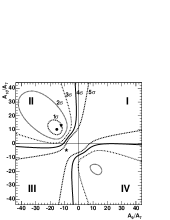
In Fig. 3, we show confidence level (CL) contours in the (, ) plane
based on the fit likelihood smeared by the systematic error, which is assumed to have a Gaussian distribution.
We also calculate an interval in at the 95% CL for the allowed region,
(4)
From this, the sign of must be negative, and the solutions in quadrants I and III
of Fig. 3 are excluded at 98.2% confidence level.
Since solutions in both quadrants II and IV are allowed, we cannot determine the sign of .
Figure 2 shows the comparison between the fit results for the negative value projected
onto the forward-backward asymmetry, and the forward-backward asymmetry distributions for several input parameters.
We exclude the new physics scenarios shown by the dotted and dot-dashed curves, which have a positive value.
Figure 3: Confidence level contours for negative . Curves show 1 to 5 contours.
The symbols show the fit (circle), SM (triangle), and -positive (star) cases.
3 Evidence of the Purely Leptonic Decay
We use a data sample containing
meson pairs collected with the Belle detector.
We use a detailed MC simulation, which fully describes the
detector geometry and response based on GEANT , to determine
the signal selection efficiency and study the background.
The signal decay is generated
by the EvtGen package .
To model the background from and continuum
production processes, large
and MC samples
corresponding to about twice the data sample
are used.
We fully reconstruct one of the mesons in
the event, referred to hereafter as the tag side (),
and compare properties of the remaining particle(s), referred to as the
signal side (), to those expected for signal and background.
In the events where a is reconstructed, we search for decays
of into a and a neutrino.
Candidate events are required to have one or three charged track(s) on the
signal side with the total charge being opposite to that of .
The lepton is identified in the five decay modes,
,
,
,
and
,
which taken together correspond to of all decays .
The muon, electron and charged pion candidates are selected based on
information from particle identification devices.
For all modes except , we reject events with
mesons on the signal side.
The most powerful variable for separating signal and background is the
remaining energy in the ECL, denoted as , which is sum of
the energy of photons that are not associated with either the
or the candidate from the
decay.
For signal events, must be either zero or a small value
arising from beam background hits, therefore, signal events peak at
low .
On the other hand background events are distributed toward higher
due to the contribution from additional neutral clusters.
The signal region is optimized for each decay mode based
on the MC simulation, and is defined by for the
, and
modes, and for
the and
modes.
The sideband region is defined by GeV
for the , and
modes, and by GeV for
the and modes.
Table 2 shows the number of events found in the sideband
region for data () and for the background MC simulation
().
Table 2 also shows the number of the background MC events
in the signal region ().
In order to validate the simulation, we use a control sample
of events (double tagged events), where the is fully reconstructed
as described above and is reconstructed in the decay chain,
(),
followed by or
where is a muon or electron.
Figure 4 shows the distribution in the
control sample for data and the MC simulation scaled to
equivalent integrated luminosity in data.
Figure 4: distribution for the both tagged events, where one is fully
reconstructed and the other is reconstructed as .
The dots with errors indicate the data. The solid histogram represents the background from
MC (), and the dashed histogram shows the contribution
from events.
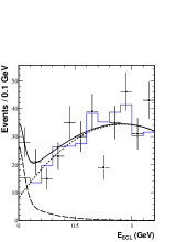
After finalizing the signal selection criteria, the signal region is examined.
Figure 5 shows the obtained distribution
when all decay modes are combined.
One can see a significant excess of events in the signal region
below GeV.
Table 2 shows the number of events observed in the
signal region () for each decay mode.
Figure 5: distributions in the data after
all selection requirements
have been applied. The data and background MC samples are represented by the points with error bars
and the solid histogram, respectively.
The solid curve shows the result of the fit with the sum of the signal shape (dashed) and background shape
(dotted).
We deduce the final results by fitting the obtained
distributions to the sum of the expected signal and background shapes.
Probability density functions (PDFs) for the signal and
for the background are constructed for each decay
mode from the MC simulation.
The signal PDF is modeled as the sum of a Gaussian function, centered at
, and an exponential function.
The background PDF, as determined from the MC simulation, is parametrized
by a second-order polynomial.
The results are listed in Table 2.
The number of signal events in the signal region deduced from the fit () is
when all decay modes are combined.
Table 2 also gives the number of background events
in the signal region deduced from the fit (), which is
consistent with the expectation from the background MC simulation
().
The branching fractions are calculated as
where is the number of
events, assumed to be half of the number of produced meson pairs.
The efficiency is defined as
,
where is the tag reconstruction efficiency for events with
decays on the signal side,
and is the event selection
efficiency listed in Table 2.
When all decay modes are combined
we obtain a branching fraction of .
The branching fraction for each decay mode is consistent within
error as shown in Table 2.
Combined
Table 2: The number of observed events in data in the sideband region ,
number of background MC events in the sideband region and the
signal region ,
number of observed events in data in the signal region ,
number of signal and background in the signal region determined by the fit,
signal selection efficiencies ,
extracted branching fraction for .
The listed errors are statistical
only.
Systematic errors for the measured branching fraction are associated with
the uncertainties in the number of , signal yields and
efficiencies.
The total fractional uncertainty of the combined measurement is
,
and we measure the branching fraction to be
The significance is when all decay modes are combined,
where the significance is defined as
,
where and denote the maximum likelihood
value and likelihood value obtained assuming zero signal events, respectively.
Here the likelihood function from the fit is convolved with a Gaussian
systematic error function in order to include the systematic uncertainty
in the signal yield.
Acknowledgments
The author wish to thank the KEKB accelerator group for the excellent operation of the KEKB
accelerator.
References
References
[1]
See, for example, G. Buchalla et al., Rev. Mod. Phys. 68, 1125 (1996).
[2] E. Lunghi et al., Nucl. Phys. B 568, 120 (2000).
[3]
J. L. Hewett and J. D. Wells, Phys. Rev. D 55, 5549 (1997); A. Ali et al., Z. Phys. C 67, 417 (1995); N. G. Deshpande et al., Phys. Lett. B 308, 322 (1993); B. Grinstein et al., Nucl. Phys. B 319, 271 (1991); W. S. Hou et al., Phys. Rev. Lett. 58, 1608 (1987).
[4]
S. Eidelman et al. (Particle Data Group),
Phys. Lett. B 592, 1 (2004).
[5]
B. Aubert (BABAR Collaboration),
Phys. Rev. D 73, 057101 (2006).
[6]
A. Abashian et al. (Belle Collaboration),
Nucl. Instrum. Methods Phys. Res., Sect. A 479, 117 (2002).
[7] D. A. Demir et al., Phys. Rev. D 66, 034015 (2002).
[8]H. H. Asatryan et al. Phys. Lett. B 507, 162 (2001).
[9] A. Ali et al., Phys. Rev. D 66, 034002 (2002).
[10]
R. Brun et al.,
GEANT3.21, CERN Report DD/EE/84-1 (1984).
[11]
See the EvtGen package home page,
http://www.slac.stanford.edu/~lange/EvtGen/.