Jet Properties from Dihadron Correlations in p+p Collisions at $\sqrt{s}$ = 200  GeV

Abstract

The properties of jets produced in $p+p$ collisions at $\sqrt{s}$=200 GeV are measured using the method of two particle correlations. The trigger particle is a leading particle from a large transverse momentum jet while the associated particle comes from either the same jet or the away-side jet. Analysis of the angular width of the near-side peak in the correlation function determines the jet fragmentation transverse momentum $j_{T\rm}$. The extracted value, $\sqrt{\left<j_{T\rm}^{2}\right>}=585\pm 6(\rm stat)\pm 15(\rm sys)\mbox{~{}MeV/$c$}$, is constant with respect to the trigger particle transverse momentum, and comparable to the previous lower $\sqrt{s}$ measurements. The width of the away-side peak is shown to be a convolution of $j_{T\rm}$ with the fragmentation variable, $z$, and the partonic transverse momentum, $k_{T\rm}$. The $\left<z\right>$ is determined through a combined analysis of the measured $\pi^{0}$ inclusive and associated spectra using jet fragmentation functions measured in $e^{+}e^{-}$ collisions. The final extracted values of $k_{T\rm}$ are then determined to also be independent of the trigger particle transverse momentum, over the range measured, with value of $\sqrt{\left<k_{T\rm}^{2}\right>}=2.68\pm 0.07(\rm stat)\pm 0.34(\rm sys)\mbox{~{}GeV/$c$}$.

I Introduction

The goal of this paper is to explore the systematics of jet production and fragmentation in $p+p$ collisions at $\sqrt{s}$=200  GeV by the method of two-particle azimuthal correlations. Knowledge of the jet-fragmentation process is useful not only as a reference measurement for a similar analysis in $Au+Au$ collisions, but can be used as a stringent test of perturbative QCD (pQCD) calculations beyond leading order.

The two-particle azimuthal correlations method worked well at ISR energies ($\sqrt{s}$=63  GeV) and below Angelis et al. (1980); Darriulat et al. (1976); Della Negra et al. (1977), where it is difficult to directly reconstruct jets, but has not been attempted at higher values of $\sqrt{s}$. This method is also suitable for jet-analysis in heavy ion data where the large particle multiplicity severely interferes with direct jet reconstruction.

With the beginning of RHIC operation, heavy-ion physics entered a new regime, where pQCD phenomena can be fully explored. High-energy partons materializing into hadronic jets can be used as sensitive probes of the early stage of heavy ion collisions. Measurements carried out during the first three years of RHIC operation at $\sqrt{s_{NN}}$=130 and 200  GeV exhibit many new and interesting features. The high-$p_{T\rm\ }$particle yield was found to be strongly suppressed in $Au+Au$ central collisions Adcox et al. (2002). Furthermore, the non-suppression of the high-$p_{T\rm\ }$particle yield in $d+Au$ induced collisions Adler et al. (2003a) confirmed that the suppression can be fully attributed to the final state interaction of high-energy partons with an extremely opaque nuclear medium formed in $Au+Au$ collisions at RHIC.

Other striking features found in RHIC data are the large asymmetry of particle azimuthal distributions which is attributed to sizable elliptic flow Adler et al. (2003b, c) and the observation of the apparent disappearance of the back-to-back jet correlation in central $Au+Au$ collisions Adler et al. (2003d).

Many of the above mentioned observations can be explained by a large opacity of the medium produced in central $Au+Au$ collisions which causes the scattered partons to lose energy via coherent (Landau-Pomeranchuk-Migdal Migdal (1956)) gluon bremsstrahlung Wang and Gyulassy (1992); Wang (1998). It is expected that the medium effect will cause the apparent modification of fundamental properties of hard-scattering like broadening of intrinsic parton transverse momentum $k_{T\rm}$ Salgado and Wiedemann (2004); Qiu and Vitev (2003) and modification of jet fragmentation Wang (2002). Thus the measurement of jet fragmentation properties and intrinsic parton transverse momentum $k_{T\rm}$ for $p+p$ collisions presented here provides a baseline for comparison to the results in heavy ion collisions, helping to disentangle the complex processes of propagation and possible fragmentation of partons within the excited nuclear medium.

This paper is organized as follows: Section II discusses the method of two-particle correlations and the relations between jet properties and the angular correlation between parton fragments. The details of the PHENIX experiment relevant to this analysis are outlined in section III. Section IV deals with the analysis of the correlation functions extracted from the $p+p$ data and an evaluation of the $\left<j_{T\rm}\right>$ and $\left<k_{T\rm}\right>$ quantities. The combined analysis of the inclusive and associated $p_{T\rm}$-distributions is discussed in section V and the sensitivity of the associated $p_{T\rm}$-distributions to the fragmentation function is discussed in section VI. Section VII presents the resulting values of the partonic transverse momenta $k_{T\rm}$ corrected for the mean momentum fraction $\left<z_{\rm t}\right>$. Section VIII summarizes the results from this paper.

II Jet angular correlations

Jets are produced in the hard scattering of two partons Berman et al. (1971a); Owens and Kimel (1978); Owens et al. (1978); Feynman et al. (1978). The overall $p+p$ hard-scattering cross section in “leading logarithm” pQCD is the sum over parton reactions $a+b\rightarrow c+d$ (e.g. $g+q\rightarrow g+q$) at parton-parton center-of-mass (c.m.) energy $\sqrt{\hat{s}}$,

$$\frac{d^{3}\sigma}{dx_{1}dx_{2}d\cos\theta^{*}}=\frac{1}{s}\sum_{ab}f_{a}(x_{1})f_{b}(x_{2})\frac{\pi\alpha_{s}^{2}(Q^{2})}{2x_{1}x_{2}}\Sigma^{ab}(\cos\theta^{*})$$ (1)

where $f_{a}(x_{1})$, $f_{b}(x_{2})$, are parton distribution functions, the differential probabilities for partons $a$ and $b$ to carry momentum fractions $x_{1}$ and $x_{2}$ of their respective protons (e.g. $u(x_{2})$), and where $\theta^{*}$ is the scattering angle in the parton-parton c.m. system. The parton-parton c.m. energy squared is $\hat{s}=x_{1}x_{2}s$, where $\sqrt{s}$ is the c.m. energy of the $p+p$ collision. The parton-parton c.m. system moves with rapidity $y=(1/2)\ln(x_{1}/x_{2})$ in the $p+p$ c.m. system.

Equation 1 gives the $p_{T\rm}$ spectrum of outgoing parton $c$ (emitted at $\theta^{*}$), which then fragments into hadrons, e.g. a $\pi^{0}$. The fragmentation function $D^{\pi^{0}}_{c}(z,\mu^{2})$ is the probability for a $\pi^{0}$ to carry a fraction $z=p^{\pi^{0}}/p^{c}$ of the momentum of outgoing parton $c$. Equation 1 must be summed over all subprocesses leading to a $\pi^{0}$ in the final state. The parameter $\mu^{2}$ is an unphysical “factorization” scale introduced to account for collinear singularities in the structure and fragmentation functions Owens (1987); Bunce et al. (2000), which will be ignored for the purposes of this paper.

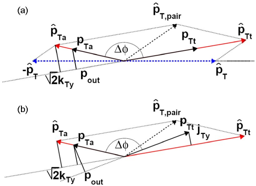
Figure 1: (color online) (a) Schematic view of a hard scattering event in the plane perpendicular to the beam. Two scattered partons with transverse momenta $\hat{p}_{T\rm}$ in the partons’ center of mass frame are seen in the laboratory frame to have a momenta $\hat{p}_{T\rm t}$ and $\hat{p}_{T\rm a}$. The net pair transverse momentum $\hat{p}_{T\rm pair}$ corresponds to the sum of the $\vec{k}_{T\rm}$-vectors of the two colliding partons. The trigger and associated jet fragments producing high-$p_{T\rm}$ particles are labeled as $p_{T\rm t}$ and $p_{T\rm a}$. The projection of $\vec{k}_{T\rm}$ perpendicular to $\hat{p}_{T\rm t}$ is labeled as $k_{T\rm y}$. The transverse momentum component of the away-side particle $\vec{p}_{T\rm a}$ perpendicular to trigger particle $\vec{p}_{T\rm t}$ is labeled as $p_{\rm out}$. (b) The same schematics as in (a), but the jet fragmentation transverse momentum component $j_{T\rm y}$ of the trigger jet is also shown.

In this formulation, $f_{a}(x_{1})$, $f_{b}(x_{2})$ and $D^{\pi^{0}}_{c}(z)$ represent the “long-distance phenomena” to be determined by experiment; while the characteristic subprocess angular distributions, $\Sigma^{ab}(\cos\theta^{*})$, and the coupling constant, $\alpha_{s}(Q^{2})=\frac{12\pi}{25\ln(Q^{2}/\Lambda^{2})}$, are fundamental predictions of QCD Cutler and Sivers (1978, 1977); Combridge et al. (1977) for the short-distance, large-$Q^{2}$, phenomena. The momentum scale $Q^{2}\sim p^{2}_{T\rm}$ for the scattering subprocess, while $Q^{2}\sim\hat{s}$ for a Compton or annihilation subprocess, but the exact meaning of $Q^{2}$ tends to be treated as a parameter rather than a dynamical quantity.

Figure 1 shows a schematic view of a hard-scattering event. The transverse momentum of the outgoing scattered parton is:

$$p_{T\rm}=p_{T\rm}^{*}={\sqrt{\hat{s}}\over 2}\;\sin\theta^{*}\qquad.$$ (2)

The two scattered partons propagate nearly back-to-back in azimuth from the collision point and fragment into the jet-like spray of final state particles (see Fig. 1(a) where only one fragment of each parton is shown).

It was originally thought that parton collisions were collinear with the $p+p$ collision axis so that the two emerging partons would have the same magnitude of transverse momenta pointing opposite in azimuth. However, it was found Della Negra et al. (1977) that each of the partons carries initial transverse momentum $\vec{k}_{T}$, originally described as “intrinsic” Feynman et al. (1977). This results in a momentum imbalance (the partons’ $p_{T\rm\ }$are not equal) and an acoplanarity (the transverse momentum of one jet does not lie in the plane determined by the transverse momentum of the second jet and the beam axes). The jets are non- collinear having a net transverse momentum $\left<p_{T\rm}^{2}\right>_{\rm pair}=2\cdot\left<k_{T\rm}^{2}\right>$.

It is important to emphasize that the $\left<k_{T\rm}\right>$ denotes the effective magnitude of the apparent transverse momentum of each colliding parton. The net transverse momentum of the outgoing parton-pair is $\sqrt{2}\cdot\left<k_{T\rm}\right>$. The naive expectation for the pure intrinsic parton transverse momentum based on nucleon constituent quark mass is about $\approx$ 300  MeV/$c$ Feynman et al. (1977); Dokshitzer et al. . However, the measurement of net transverse momenta of diphotons, dileptons or dijets over a wide range of center-of-mass energies gives $\left<k_{T\rm}\right>$ as large as 5 GeV/$c$ Apanasevich et al. (1999). It is common to think of the net transverse momentum of a dilepton or dijet pair as composed of 3 components:

$${\left<p_{T\rm}^{2}\right>_{\rm pair}\over 2}=\left<k_{T\rm}^{2}\right>=\left<k_{T\rm}^{2}\right>_{\rm intrinsic}+\left<k_{T\rm}^{2}\right>_{\rm soft}+\left<k_{T\rm}^{2}\right>_{\rm NLO}\;\;,$$ (3)

where the intrinsic part refers to the possible “fermi motion” of the confined quarks or gluons inside a proton, the NLO part refers to the power law tail at large values of $p_{T_{pair}}$ due to the radiation of an initial state or final state hard gluon, which is divergent as the momentum of the radiated gluon goes to zero, and the soft part refers to the actual Gaussian-like distribution observed as $p_{T_{pair}}\rightarrow 0$, which is explained by resummation Kulesza et al. (2003).

In the discussion below we will assume that the two components of the vector $\vec{k}_{T\rm}$, $k_{T\rm x}$ and $k_{T\rm y}$ are Gaussian distributed with equal standard deviations $\sigma_{\rm 1parton,1d}$, in which case $k^{2}_{T\rm}$=$k^{2}_{T\rm x}$+$k^{2}_{T\rm y}$ is distributed according to a 2-dimensional (2D) Gaussian Apanasevich et al. (1999). For the net transverse momentum of the jet pair, $\left<p_{T\rm}^{2}\right>_{\rm pair}=\sigma^{2}_{\rm 2partons,2d}=2\sigma^{2}_{\rm 1parton,2d}$. Note that the principal difference between the 1 and 2 dimensional Gaussians is that $\left<k_{T\rm x}\right>$=$\left<k_{T\rm y}\right>$=0, while $\left<k_{T\rm}\right>\neq 0$ since $\vec{k}_{T\rm}$ is a 2D radius vector.

The two components of $k_{T\rm}$ result in different experimentally measurable effects. $k_{T\rm y}$ leads to the acoplanarity of the dijet pair while $k_{T\rm x}$ makes the momenta of the jets unequal which results in the smearing of the steeply falling $p_{T\rm}$ spectrum. This causes the measured inclusive jet or single particle cross section to be larger than the pQCD value given by Eq. 1. This was observed in the original discovery of high $p_{T\rm}$ particle production at the CERN ISR in 1972 Busser et al. (1973) and led to much confusion until the existence and effects of $k_{T\rm}$ were understood.

Before the advent of QCD, the invariant cross section for the hard-scattering of the electrically charged partons of deeply inelastic scattering was predicted for $p+p$ collisions to follow a general scaling form: Berman et al. (1971b); Blankenbecler et al. (1972)

$$E\frac{d^{3}\sigma}{d^{3}p}=\frac{1}{p_{T\rm}^{n}}F({x_{T}})=\frac{1}{\sqrt{s}^{n}}G({x_{T}})\qquad,$$ (4)

where $x_{T}=2p_{T\rm}/\sqrt{s}$. The cross section has two factors, a function $F({x_{T}})$ ($G({x_{T}})$) which ‘scales’, i.e. depends only on the ratio of momenta, and a dimensioned factor, ${1/p_{T\rm}^{n}}$ ($1/\sqrt{s}^{\,n}$), where $n$ equals 4 for QED, and for LO-QCD (Eq. 4), analogous to the $1/q^{4}$ form of Rutherford Scattering. The structure and fragmentation functions are all in the $F(x_{T})$ ($G(x_{T})$) term. The original high $p_{T\rm}$ measurements at CERN Busser et al. (1973) and Fermilab Antreasyan et al. (1979), showed beautiful $x_{T}$ scaling, but with a value of $n=8$ instead of $n=4$, for values of $3\leq p_{T\rm}\leq 7$ GeV/c. Later measurements at larger $p_{T\rm}$ showed the correct scaling in agreement with pQCD and it was realized that the value $n=8$ at lower values of $p_{T\rm}$ and $\sqrt{s}$ was produced by the $k_{T\rm x}$ smearing Owens and Kimel (1978); Owens et al. (1978). More recently, the deviation of $\pi^{0}$ and direct photon inclusive cross sections measurements from pQCD predictions has been used to derive the values of $k_{T\rm}$ required to bring the measured and smeared pQCD predictions into agreement. Apanasevich et al. (1999).

A more direct method to determine $k_{T\rm y}$ is to measure the acoplanarity of the dijet pair. Such measurements were originally performed at the CERN-ISR using two particle correlations  Angelis et al. (1980); Della Negra et al. (1977); Darriulat et al. (1976); Feynman et al. (1977). The same method will be used in the present work.

Hard-scattering in $p+p$ collisions at $\sqrt{s}=200$ GeV is detected by triggering on a $\pi^{0}$ with transverse momentum $p_{T_{t}}\geq 3$ GeV/c; and the properties of jets are measured using the method of two particle correlations. The trigger $\pi^{0}$ is a leading particle from a large transverse momentum jet while the associated particle comes from either the same jet or the away-side jet. We will analyze an outgoing dijet pair, with trigger jet transverse momentum magnitude $\hat{p}_{T\rm t}$ which fragments to a trigger particle with transverse momentum $\vec{p}_{T\rm t}$, and an away-side jet transverse momentum magnitude of $\hat{p}_{T\rm a}$ which fragments to a particle with transverse momentum $\vec{p}_{T\rm a}$. The average transverse momentum component of the away-side particle $\vec{p}_{T\rm a}$ perpendicular to trigger particle $\vec{p}_{T\rm t}$ in the azimuthal plane is labeled as $p_{\rm out}$. If the magnitude of the jet transverse fragmentation momentum $j_{T\rm}$ (Fig. 1(a) is neglected, the magnitude of $\sqrt{2}k_{T\rm y}$ can be related to $p_{\rm out}$: $\sqrt{2}k_{T\rm y}=p_{\rm out}\,\hat{p}_{T\rm a}/p_{T\rm a}\equiv p_{\rm out}/z_{\rm a}$. Thus the measurement of $p_{\rm out}$ and the knowledge of the fragmentation variable ($z_{\rm a}$) determines the magnitude of the parton’s transverse momentum $k_{T\rm}$.

The smearing of the steeply falling parton $\hat{p}_{T\rm}$ spectrum by the $k_{T\rm x}$ distribution tends to make the trigger jet transverse momentum $\hat{p}_{T\rm t}$ larger than the away jet transverse momentum $\hat{p}_{T\rm a}$ . The component of the net transverse momentum of the parton pair along the trigger direction is smeared by $\sqrt{2}\,k_{T\rm x}$ such that:

$$\left<(\hat{p}_{T\rm t}-\hat{p}_{T\rm ax})^{2}\right>=2\,\left<k_{T\rm x}^{2}\right>=\left<k_{T\rm}^{2}\right>\qquad.$$ (5)

For a flat $\hat{p}_{T\rm}$ spectrum, the smearing would average to zero so that there would be no net shift in the transverse momentum spectrum:

$$\left<\hat{p}_{T\rm t}-\hat{p}_{T\rm}\right>=\left<\hat{p}_{T\rm}-\hat{p}_{T\rm ax}\right>=0\qquad.$$ (6)

However, due to the steeply falling $\hat{p}_{T\rm}$ spectrum, the $k_{T\rm x}$ smearing results in a net imbalance of the jet-pair towards the trigger direction. In the limit when $k_{T\rm}$ is collinear with the trigger jet and with the requirement of the Lorentz invariance of $\hat{s}$ ($\hat{p}^{2}_{T\rm}$=$\hat{p}_{T\rm t}$$\hat{p}_{T\rm a}$) it is easy to see that

$$\left<\hat{p}_{T\rm t}-\hat{p}_{T\rm}\right>=\left<{\hat{p}_{T\rm t}\over\hat{p}_{T\rm}}(\hat{p}_{T\rm}-\hat{p}_{T\rm a})\right>\simeq{1\over 2}{\left<\hat{p}_{T\rm t}-\hat{p}_{T\rm a}\right>}>0\;.$$ (7)

We denote the imbalance of $\hat{p}_{T\rm a}$ and $\hat{p}_{T\rm t}$ by the quantity

$$\hat{x}_{\rm h}={\left<\hat{p}_{T\rm a}\right>/\left<\hat{p}_{T\rm t}\right>}.$$ (8)

Jet fragments have a momentum $\vec{j}_{T\rm\ }$perpendicular to the partonic transverse momentum (Fig. 1(b). This vector is again a two-dimensional vector with one component perpendicular to the jet transverse axis, $\vec{\hat{p}}_{T\rm,}$ in the transverse plane and the other component perpendicular to the jet transverse axis in the longitudinal plane (defined by the beam and jet axes). The component of $\vec{j}_{T\rm\ }$projected onto the azimuthal plane is labeled as $j_{T\rm y}$. The magnitude of $\left<j_{T\rm y}\right>$, the mean value of $j_{T\rm}$ projected into the plane perpendicular to the jet thrust (see App.A.1), measured at lower energies Angelis et al. (1980) has been found to be $p_{T\rm}$ independent and $\approx$ 400 MeV/$c$, consistent with measurements in $e^{+}e^{-}$ collisions Darriulat (1980); Adachi et al. (1999).

This analysis uses two-particle azimuthal correlation functions to measure the average relative angles between a trigger $\pi^{0}$ and an associated charged hadron. The angular width of the near- and away-side peak in the correlation function is used to extract the value of $\left<j_{T\rm}^{2}\right>$ and $\hat{x}_{\rm h}^{-1}\left<z_{\rm t}\right>\sqrt{\left<k_{T\rm}^{2}\right>}$. An analysis of the associated yields is used to extract the fragmentation function which provides the $\left<z_{\rm t}\right>$ and $\left<z_{\rm a}\right>$ values used for $\left<k_{T\rm}^{2}\right>$ extraction. The details on the PHENIX experiment relevant to this analysis follow.

III Experimental Details

The PHENIX experiment consists of four spectrometer arms - two around mid-rapidity (the central arms) and two at forward rapidity (the muon arms) - along with a set of global detectors. The layout of the PHENIX experiment during RHIC Run-3 is shown in Fig. 2.

Each central arm covers the pseudorapidity range $|\eta|<0.35$ and 90 degrees in azimuthal angle $\phi$. In each of the central arms, charged particles are tracked by a drift chamber (DC) positioned from 2.0 to 2.4m radially outward from the beam axis and 2 or 3 layers of pixel pad chambers (PC1, PC2, PC3 located at 2.4m, 4.2m, 5m in the radial direction, respectively). Particle identification is provided by ring imaging Čerenkov counters (RICH), a time of flight scintillator wall (TOF), and two types of electromagnetic calorimeters (EMCal), lead scintillator (PbSc) and lead glass (PbGl). The magnetic field for the central arm spectrometers is axially symmetric around the beam axis. Its component parallel to the beam axis has an approximately Gaussian dependence on the radial distance from the beam axis, dropping from 0.48 T at the center to 0.096 T (0.048 T) at the inner (outer) radius of the DC. A pair of Zero-Degree Calorimeters (ZDC) and a pair of Beam-Beam Counters (BBC) were used for global event characterization. Further details about the design and performance of PHENIX can be found in Adcox et al. (2003a); Aphecetche et al. (2003a); Adcox et al. (2003b).

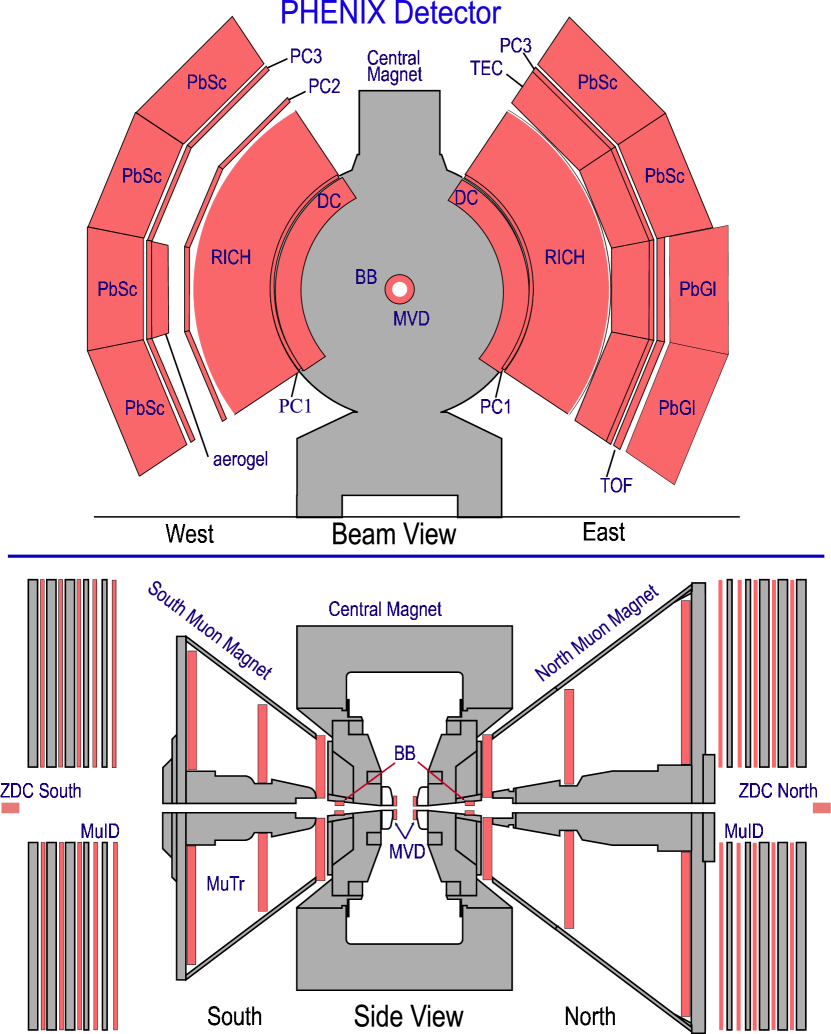
Figure 2: (color online) The PHENIX experimental layout for the Au+Au run in 2003. The top panel shows the PHENIX central arm spectrometers viewed along the beam axis. The bottom panel shows a side view of the PHENIX muon arm spectrometers and the position of the global detectors (BBC and ZDC).

A $p+p$ data sample corresponding to an integrated luminosity 0.35 pb^-1 at $\sqrt{s}=200$ GeV has been used for the present analysis. It contains a minimum bias (MB) sample of 121M events and a high-$p_{T\rm\ }$triggered sample of 50M events. The MB trigger is obtained from the charge multiplicity in the two BBCs situated at large pseudo-rapidity ($\eta\approx\pm(3.0-3.9)$). The BBCs were also used to determine the collision vertex, which is limited to a $\pm$30cm range in this analysis. The high-$p_{T\rm\ }$trigger requests an additional discrimination on sums of the analog signals from non-overlapping, 2x2 groups of adjacent EMCal towers situated at mid-rapidity ($|\eta|<0.35$) equivalent to an energy deposition of 750 MeV Adler et al. (2003e). The analysis has been performed separately on the two data sets and no trigger selection bias was found within the quoted errors.

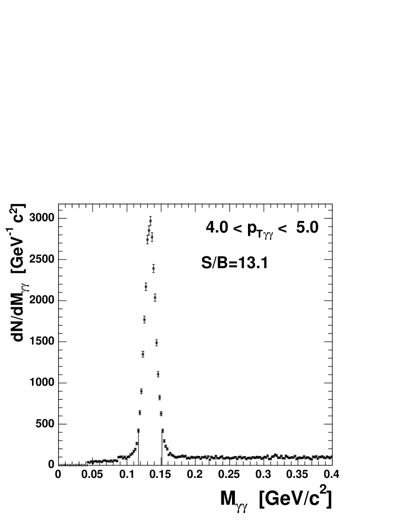
Figure 3: The measured $\gamma\gamma$ invariant mass distribution for pair $p_{T\rm\ }$in $4<p_{T\gamma\gamma}<5$ GeV/$c$. The peak is fitted with a Gaussian. The signal/background ratio within 2$\sigma$ of the mean ranges from $\approx$ 6 at $p_{T\rm}$ of 3 GeV/$c$ up to $\approx$ 15 at 8 GeV/$c$.

Neutral pions, which are used as trigger particles, are detected by the reconstruction of their $\gamma\gamma$ decay channel. Photons are detected in the EMCal, which has a timing resolution of $\approx$ 100 $ps$ (PbSc) and $\approx$ 300 $ps$ (PbGl) and energy resolution of $\sigma_{E}/E$=1.9%$\oplus$8.2%/$\sqrt{E(GeV)}$ (PbSc) and $\sigma_{E}/E$=0.8%$\oplus$8.4%/$\sqrt{E(GeV)}$ (PbGl). In order to improve the signal/background ratio we require the minimum hit energy $>0.3$  GeV, a shower profile cut as described in Aphecetche et al. (2003b), and no accompanying hit in the RICH detector, which serves as a veto for conversion electrons. A sample of the invariant mass distribution of photon pairs detected in the EMCal is shown in Fig. 3.

Charged particles are reconstructed in each PHENIX central arm using a drift chamber, followed by two layers of multiwire proportional chambers with pad readout Adcox et al. (2003a). Particle momenta are measured with a resolution $\delta p/p=0.7\%\oplus 1.1\%p$ (GeV/c). A confirmation hit is required in PC3. We also require that no signal in the RICH detector is associated with these tracks. These requirements eliminate charged particles which do not originate from the event vertex, such as beam albedo and weak decays, as well as conversion electrons.

High momentum charged pions (above the RICH Čerenkov threshold) are identified using the RICH and EMCal detectors. Candidate tracks must be associated with a hit in the RICH Aizawa et al. (2003), which corresponds to a minimum momentum of 18 MeV/$c$ for electrons, 3.5 GeV/$c$ for muons, and 4.9 GeV/$c$ for charged pions. In a previous PHENIX publication Adler et al. (2004), we have shown that charged particles with reconstructed $p_{T\rm\ }$above 4.9  GeV/$c$, which have an associated hit in the RICH, are dominantly charged pions and background electrons from photon conversions albedo. The efficiency for detecting charged pions rises quickly past 4.9  GeV/$c$, reaching an efficiency of $>90\%$ at $p_{T\rm}>6$  GeV/$c$.

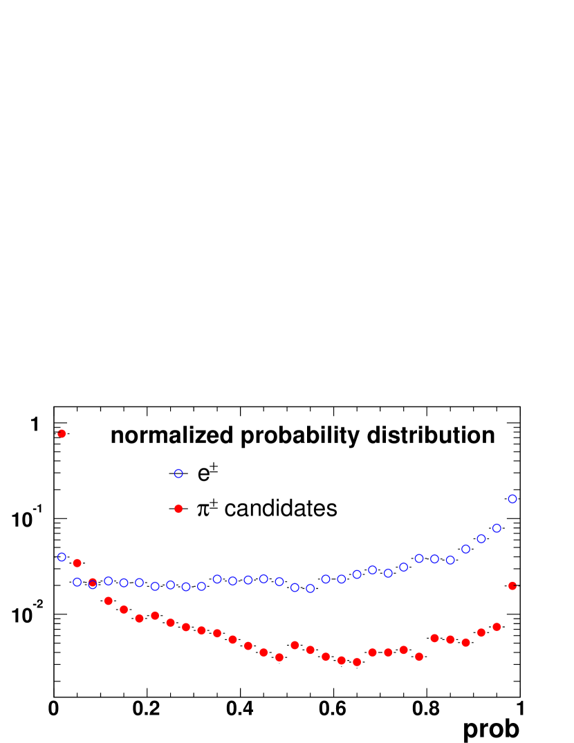
Figure 4: (color online) The probability distribution for charged pion candidates and electrons derived from the EM shower shape using identified electrons and pions. The integrals have been normalized to one.

To reject the electron background in the charged pion candidates, the shower information at the EMCal is used. Since most of the background electrons are genuine low $p_{T}$ particles that were mis-reconstructed as high $p_{T\rm\ }$particles, simply requiring a large deposition of shower energy in the EMCal is effective in suppressing the electron background. In this analysis, a momentum- dependent energy cut on the EMCal is applied

$$E>0.3+0.15p_{T}.$$ (9)

In addition to this energy cut, the shower shape information Aphecetche et al. (2003b) is used to further separate the broad hadronic showers from the narrow electromagnetic showers and hence reduce the conversion backgrounds. The difference of the EM shower and hadronic shower is typically characterized by a $\chi^{2}$ variable Aphecetche et al. (2003b),

$$\chi^{2}=\sum_{i}\frac{(E^{meas}_{i}-E^{pred}_{i})^{2}}{\sigma_{i}^{2}},$$ (10)

where $E^{meas}_{i}$ is the energy measured at tower $i$ and $E^{pred}_{i}$ is the predicted energy for an electromagnetic particle of total energy $\sum_{i}E^{meas}_{i}$.

In this analysis we use the probability calculated from this $\chi^{2}$ value for an EM shower, ranging from 0 to 1 with a flat distribution expected for an EM shower, and a peak around 0 for an hadronic shower.

Figure 4 shows the probability distribution for pion and electron candidates, each normalized to one. The pion candidates were required to pass the energy cut and the electrons were selected using particle ID cuts similar to that used in Adler et al. (2005). The electron distribution is relatively flat, while the charged pion distribution peaks at 0. A cut of shower shape probability $<0.2$ selects pions above the energy cut with an efficiency of $\gtrsim 80$%. Detailed knowledge of the pion efficiency is not necessary, since we present in this paper the per-trigger pion conditional-yield distributions, for which this efficiency cancels out.

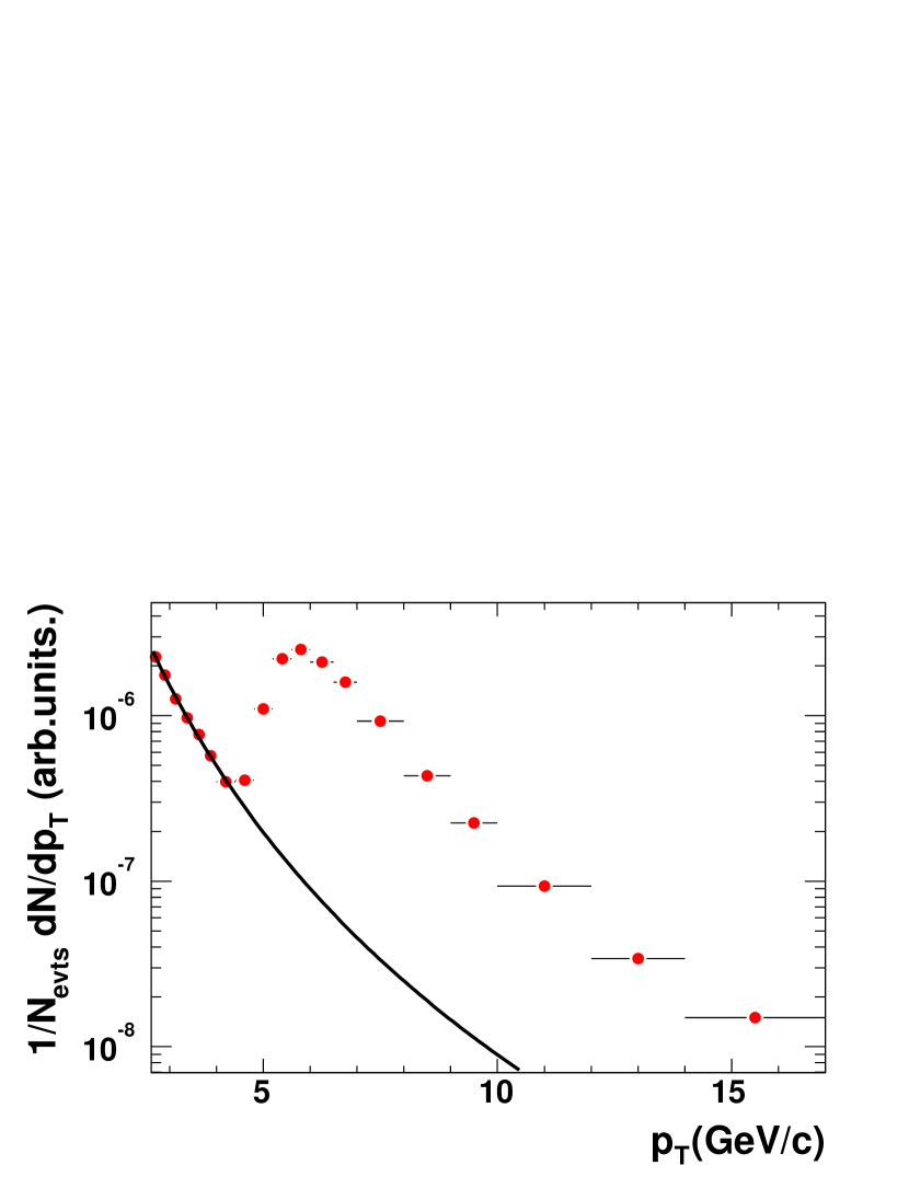
Figure 5: (color online) The raw charged pion transverse momentum spectrum, with the final cuts applied. The level of the remaining background is estimated from an extrapolation from low-p_T and is shown as a black line.

Since the energy and shower shape cuts are independent of each other, we can fix one cut and then vary the second to check the remaining background level from conversions. The energy cut in Eq. (9) is chosen such that the raw pion yield is found to be insensitive to the variation in the shower shape probability. Figure 5 shows the raw pion spectra for EMCal-RICH triggered events as a function of $p_{T}$, with the above cuts applied. The pion turn on from $4.9-7$ GeV/$c$ is clearly visible. Below $p_{T}$ of 5 GeV/$c$, the remaining background comes mainly from the random association of charged particles with hits in the RICH detector. The background level is less than 5% from $5-16$ GeV/$c$, which is the $p_{T}$ range for the charged pion data presented in this paper.

IV Correlation function

The analysis uses two-particle azimuthal correlation functions between a neutral pion and an associated charged hadron to measure the distribution of the azimuthal angle difference $\Delta\phi=\phi_{t}-\phi_{a}$ (see Fig. 6). Whenever a $\pi^{0}$ was found in an event, the real, $dN_{\rm uncorr}/d\Delta\phi$, and mixed, $dN_{\rm mix}/d\Delta\phi$, distributions for given $p_{T\rm t}$ ($\pi^{0}$) and $p_{T\rm a}$ (charged hadron) were accumulated (left panel of Fig. 6). Mixed events were obtained by randomly selecting each member of a particle pair from different events having similar vertex position. Then the mixed event distribution was used to correct the correlation function for effects of the limited PHENIX azimuthal acceptance and for the detection efficiency, to the extent that it remains constant over the data sample.

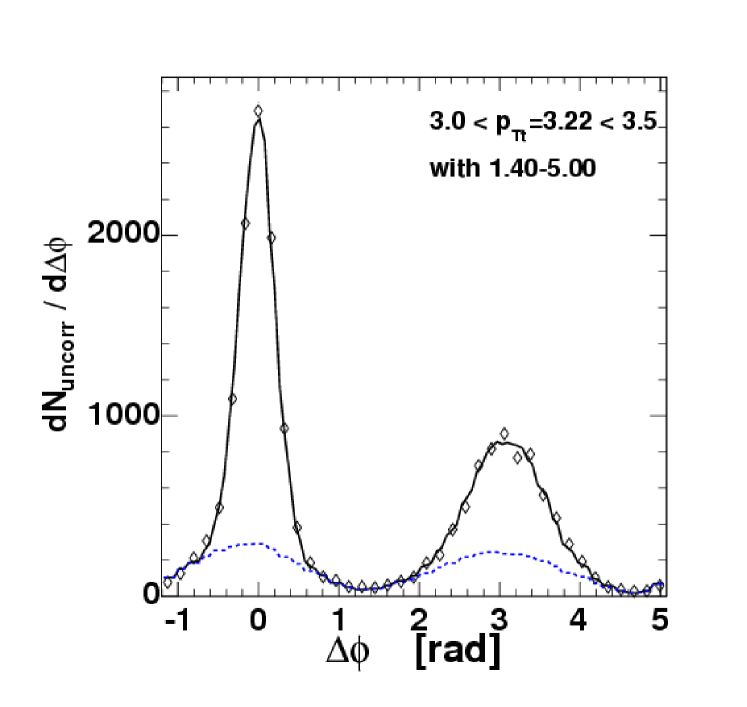
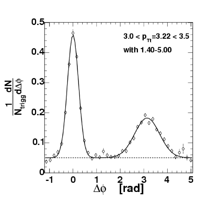
Figure 6: (color online) An example of the correlation functions for 3$<p_{T\rm t}<$3.5  GeV/$c$ and associated particles in 1.4$<p_{T\rm a}<$5  GeV/$c$. (upper) Unnormalized pair-yield distribution plotted with the fit function which is two Gaussians modulated by the pair detection efficiency derived from the mixed distribution (blue dashed line). (lower) Per $\pi^{0}$ trigger yield distribution corrected for the pair detection efficiency. Dashed line represents the constant term in the fit.

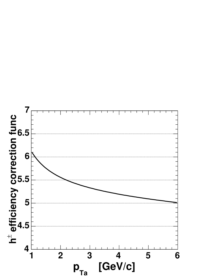
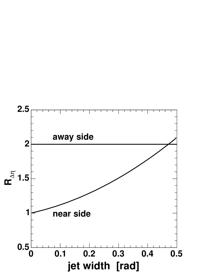
Figure 7: (upper) Inclusive charged hadron efficiency correction function. (lower) $\eta$ acceptance correction factor for loss of jet pairs outside the limited $\eta$-acceptance of the PHENIX experiment.

We fit the raw $dN_{\rm uncorr}/d\Delta\phi$ distribution with the product

$${dN_{\rm uncorr}\over d\Delta\phi}=$$ (11)

$${1\over\cal{N}}{dN_{\rm mix}\over d\Delta\phi}\cdot\left(C_{0}+C_{1}\cdot f_{\rm near}(\Delta\phi)+C_{2}\cdot f_{\rm away}(\Delta\phi)\right)$$

where the mixed event distribution is normalized to $2\pi$ ($\mathcal{N}=\sum dN^{i}_{\rm mix}/d\Delta\phi$ see blue dashed line on the left panel of Fig. 6), $C_{0-2}$ are constant factors to be determined from the fit, $f_{\rm near}(\Delta\phi)$ and $f_{\rm away}(\Delta\phi)$ are the near- and away-side peak fit functions respectively. Traditionally, the Gaussian functions, around $\Delta\phi=0$ and around $\Delta\phi=\pi$, are used for $f_{\rm near}(\Delta\phi)$ and $f_{\rm away}(\Delta\phi)$. This leaves a total of five free parameters to be determined - the areas and widths of the above two Gaussians: $Y_{\rm N}$, $\sigma_{\rm N}$ for the near-angle component and $Y_{\rm F}$, $\sigma_{\rm A}$ for the away-angle component and the constant term describing an uncorrelated distribution of particle pairs which are not associated with jets. However, the assumption of the Gaussian shape of the angular correlation induced by jet fragmentation is justified only in the high-$p_{T\rm\ }$region where the relative angles are small. In order to access also a lower $p_{T\rm\ }$region we used an alternative parameterization of $f_{\rm near}(\Delta\phi)$ and $f_{\rm away}(\Delta\phi)$ which will be discussed later in the text.

The normalized correlation function was constructed as a ratio of real and mixed distributions multiplied by $\eta$-acceptance correction factor $R_{\Delta\eta}$, divided by $p_{T\rm}$-dependent efficiency correction $\epsilon(p_{T\rm})$ (see left panel of Fig. 7) and divided by the number of $\pi^{0}$ triggers.

$${1\over N_{\rm trigg}}{dN\over d\Delta\phi}={R_{\Delta\eta}\over N_{\rm trigg}\,\epsilon(p_{T\rm})}{dN_{\rm uncorr}(\Delta\phi)/d\Delta\phi\over dN_{\rm mix}(\Delta\phi)/d\Delta\phi}\cdot\cal{N}.$$ (12)

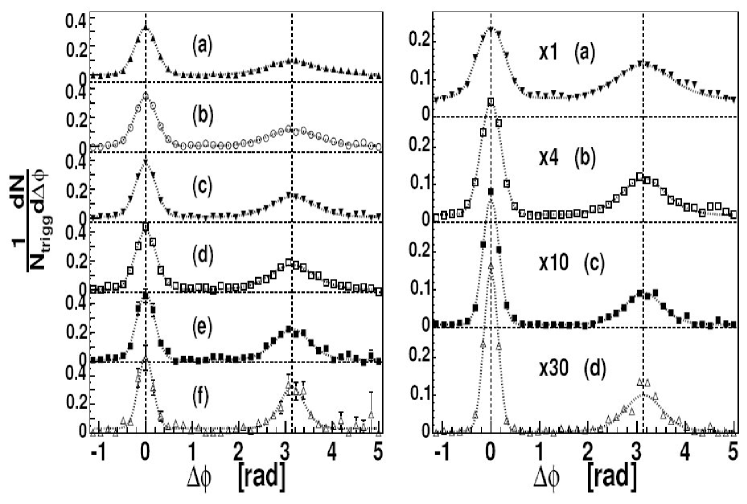
Figure 8: (left) Measured yield of charged hadrons with away-side transverse momentum $1.4<p_{T\rm a}<5.0\mbox{~{}GeV/$c$}$ associated with a trigger $\pi^{0}$ of transverse momenta given in in Table 1. (right) Measured yield of charged hadrons associated with a trigger $\pi^{0}$ of fixed transverse momentum $3.0<p_{T\rm t}<10.0\mbox{~{}GeV/$c$}$ and the away-side transverse momenta given in Table 1. The dashed lines corresponds to the fit of two Gaussian functions representing the trigger (t) jet and away-side (a) jet correlation. The $\chi^{2}$(DOF) $\sigma_{\rm N}$ and $\sqrt{\left<p_{\rm out}^{2}\right>}$ values extracted from these fits are tabulated in Table 1.

Table 1: The $\chi^{2}$(DOF) $\sigma_{\rm N}$ and $\sqrt{\left<p_{\rm out}^{2}\right>}$ values extracted for the correlation function shown in Fig. 8. All units in rad and  GeV/$c$. Only the statistical errors are shown.

$1.4<p_{T\rm a}<5.0\mbox{~{}GeV/$c$}$				$3.0<p_{T\rm t}<10.0\mbox{~{}GeV/$c$}$
$p_{T\rm t}$  GeV/$c$	$\chi^{2}$(DOF=34)	$\sigma_{\rm N}$	$\sqrt{\left<p_{\rm out}^{2}\right>}$	$p_{T\rm a}$	$\chi^{2}$(DOF=34)	$\sigma_{\rm N}$	$\sqrt{\left<p_{\rm out}^{2}\right>}$
(a) $2.5-3.0$	69.4	0.26 $\pm$ 4E-03	1.17 $\pm$ 0.07	(a) $1.0-2.0$	188.4	0.29 $\pm$ 4E-03	0.87 $\pm$ 0.03
(b) $3.0-3.5$	79.6	0.24 $\pm$ 4E-03	1.19 $\pm$ 0.05	(b) $2.0-3.0$	63.2	0.21 $\pm$ 3E-03	1.16 $\pm$ 0.04
(c) $3.5-4.5$	61.2	0.22 $\pm$ 3E-03	1.04 $\pm$ 0.04	(c) $3.0-4.0$	50.3	0.16 $\pm$ 4E-03	1.36 $\pm$ 0.06
(d) $4.5-5.5$	52.7	0.22 $\pm$ 6E-03	1.08 $\pm$ 0.06	(d) $4.0-5.0$	63.2	0.14 $\pm$ 4E-03	1.69 $\pm$ 0.13
(e) $5.5-6.5$	38.4	0.20 $\pm$ 8E-03	0.90 $\pm$ 0.06
(f) $6.5-8.0$	31.6	0.16 $\pm$ 1E-02	0.64 $\pm$ 0.06

The $R_{\Delta\eta}$ correction factor which accounts for limited $\eta$ acceptance of the PHENIX experiment (see right panel of Fig. 7) for the the near-side yield, with an assumption that the angular jet width is the same in $\Delta\eta$ and in $\Delta\phi$, can be written as

$$R_{\Delta\eta}={1\over{1\over\sqrt{2\pi\sigma_{\rm N}^{2}}}\int_{-0.7}^{0.7}\exp\left(-{\Delta\eta\over 2\sigma_{\rm N}^{2}}\right)acc(\Delta\eta)d\eta},$$ (13)

where $acc(\Delta\eta)$ represent the PHENIX pair acceptance function in $|\Delta\eta|$. It can be obtained by convolving two flat distributions in $|\Delta\eta|<$0.35, so $acc(\Delta\eta)$ has a simple triangular shape: $acc(\Delta\eta)=(0.7-|\Delta\eta|)/0.7$. For the away-side yield the corresponding $R_{\Delta\eta}$ is

$$R_{\Delta\eta}={2(0.7)\over{1\over\sqrt{2\pi\sigma_{\rm N}^{2}}}\int_{-0.7}^{0.7}acc(\Delta\eta)d\eta}=2.$$ (14)

$R_{\Delta\eta}$ equals 2, because the pair efficiency has a triangular shape in $|\Delta\eta|<$0.7, which results in 50% average efficiency when the real jet pair distribution is flat in $|\Delta\eta|<$0.7. Normalized correlation functions for various $p_{T\rm t}$ and $p_{T\rm a}$ are shown in Fig. 8.

For two particles with transverse momenta $p_{T\rm t}$, $p_{T\rm a}$ from the same jet, the width of the near-side correlation distribution can be related to the RMS value of the $j_{T\rm}$ vector component, $j_{T\rm y}$, perpendicular to the parton momentum as

$$\sigma_{\rm N}^{2}=\left<\Delta\phi^{2}\right>=\left<\left({j_{T\rm y}\over p_{T\rm a}}\right)^{2}+\left({j_{T\rm y}\over p_{T\rm t}}\right)^{2}\right>,$$ (15)

where we assume $\left<j_{T\rm y}^{2}\right>$$\ll$$p^{2}_{T\rm t}$ and $p^{2}_{T\rm a}$ and thus the arc-sine function can be approximated by its argument and we can solve for

$$\sqrt{\left<j_{T\rm}^{2}\right>}=\sqrt{2\,\left<j_{T\rm y}^{2}\right>}\simeq\sqrt{2}{p_{T\rm t}\,p_{T\rm a}\over\sqrt{p_{T\rm t}^{2}+p_{T\rm a}^{2}}}\;\sigma_{\rm N}\quad.$$ (16)

In order to extract $\left<|k_{T\rm y}|\right>$, or $\left<k_{T\rm}^{2}\right>$, we start with the relation Feynman et al. (1977); Angelis et al. (1980) between the magnitude of $p_{\rm out}$,(see Fig. 1)

$$p_{\rm out}=p_{T\rm a}\,\sin\Delta\phi,$$ (17)

which is the transverse momentum component of the away-side particle $\vec{p}_{T\rm a}$ perpendicular to trigger particle $\vec{p}_{T\rm t}$ in the azimuthal plane (see Fig. 1), and $k_{T\rm y}$:

$$\left<|p_{\rm out}|\right>^{2}=x_{\rm E}^{2}\left[2\left<|k_{T\rm y}|\right>^{2}+\left<|j_{T\rm y}|\right>^{2}\right]+\left<|j_{T\rm y}|\right>^{2},$$ (18)

where

$$x_{\rm E}=-{\vec{p}_{T\rm t}\cdot\vec{p}_{T\rm a}\over p_{T\rm t}^{2}}=-{p_{T\rm a}\,\cos{\Delta\phi}\over p_{T\rm t}}\simeq{z_{\rm a}\,\hat{p}_{T\rm a}\over z_{\rm t}\,\hat{p}_{T\rm t}}$$ (19)

represents the fragmentation variable of the away-side jet. Darriulat et al. (1976); Della Negra et al. (1977) We note however, that Feynman et al. (1977) explicitly neglected $\left<z_{\rm t}\right>=\left<p_{T\rm t}/\hat{p}_{T\rm t}\right>$ in the formula at ISR energies, where $\left<z_{\rm t}\right>\simeq$ 0.85, while it is not negligible at $\sqrt{s}$=200 GeV. Furthermore, as mentioned earlier, the average values of trigger and associated jet momenta are generally not the same. There is a systematic momentum imbalance due to $k_{T\rm}$-smearing of the steeply falling parton momentum distribution. The event sample with a condition of $p_{T\rm t}$$>$$p_{T\rm a}$ is dominated by configurations where the $k_{T\rm}$-vector is parallel to the trigger jet and antiparallel to the associated jet and $\left<\hat{p}_{T\rm t}-\hat{p}_{T\rm a}\right>\neq 0$. Here we introduce the hadronic variable $x_{\rm h}$ in analogy to the partonic variable $\hat{x}_{\rm h}$

$$x_{\rm h}\equiv{p_{T\rm a}\over p_{T\rm t}}\mbox{\hskip 14.22636pt}\hat{x}_{\rm h}=\hat{x}_{\rm h}(\left<k_{T\rm}^{2}\right>,x_{\rm h})\equiv{\left<\hat{p}_{T\rm a}\right>\over\left<\hat{p}_{T\rm t}\right>}$$ (20)

The detailed discussion on the magnitude of this imbalance is given later. In order to derive the relation between the magnitude of $p_{\rm out}$ and $k_{T\rm}$ let us first consider the simple case where we have neglected both trigger and associated $\left<j_{T\rm}\right>$ (see panel (a) on Fig. 1). In this case one can see that

$$\left<|p_{\rm out}|\right>|_{j_{T\rm t}=j_{T\rm a}=0} \equiv \left<|p_{\rm out}|\right>_{00}=$$

$$= \sqrt{2}\left<|k_{T\rm y}|\right>{p_{T\rm a}\over\left<\hat{p}_{T\rm a}\right>}=$$

$$= \sqrt{2}\left<|k_{T\rm y}|\right>\left<z_{\rm t}\right>{x_{\rm h}\over\hat{x}_{\rm h}}\;.$$

Rewriting the formula for $p_{\rm out}$ in terms of RMS we get

$$\sqrt{\left<p_{\rm out}^{2}\right>}_{00}=\left<z_{\rm t}\right>\sqrt{\left<k_{T\rm}^{2}\right>}\,{x_{\rm h}\over\hat{x}_{\rm h}}\qquad,$$

where we have taken $\left<k_{T}^{2}\right>$=$\left<2k_{T_{y}}^{2}\right>$ .

However, the jet fragments are produced with finite jet transverse momentum $j_{T\rm}$. The situation when the trigger particle is produced with $j_{T\rm ty}$$>0$  GeV/$c$ and the associated particle with $j_{T\rm ay}$=0  GeV/$c$ is shown in Fig. 1b. The $p_{\rm out}$ vector picks up an additional component

$$\left<p_{\rm out}^{2}\right>|_{j_{T\rm t}>0,\,j_{T\rm a}=0}=$$

$$= \left[\left<p_{\rm out}^{2}\right>_{00}+{\left<j_{T\rm ty}^{2}\right>\over p^{2}_{T\rm t}}(p^{2}_{T\rm a}-\left<p_{\rm out}^{2}\right>_{00})\right]{p^{2}_{T\rm t}-\left<j_{T\rm ty}^{2}\right>\over p^{2}_{T\rm t}}$$

With an assumption of $j_{T\rm ty}\ll p_{T\rm t}$ we found that

$$\left<p_{\rm out}^{2}\right>|_{j_{T\rm t}>0,\,j_{T\rm a}=0}=x_{\rm h}^{2}\left[\left<z_{\rm t}\right>^{2}\left<k_{T\rm}^{2}\right>\,{1\over\hat{x}_{\rm h}^{2}}+\left<j_{T\rm ty}^{2}\right>\right]$$

We include $j_{T\rm a}$ in the same approximation, $j_{T\rm ay}\ll p_{T\rm a}$, i.e. collinearity of $j_{T\rm a}$ and $p_{\rm out}$  with result

$$\left<p_{\rm out}^{2}\right>=x_{\rm h}^{2}\left[\left<z_{\rm t}\right>^{2}\left<k_{T\rm}^{2}\right>\,{1\over\hat{x}_{\rm h}^{2}}+\left<j_{T\rm ty}^{2}\right>\right]+\left<j_{T\rm ay}^{2}\right>$$ (21)

and we solve for $\left<z_{\rm t}\right>\sqrt{\left<k_{T\rm}^{2}\right>}$/$\hat{x}_{\rm h}$

$${\left<z_{\rm t}\right>\sqrt{\left<k_{T\rm}^{2}\right>}\over\hat{x}_{\rm h}}={1\over x_{\rm h}}\sqrt{\left<p_{\rm out}^{2}\right>-\left<j_{T\rm ay}^{2}\right>-x_{\rm h}^{2}\left<j_{T\rm ty}^{2}\right>}\qquad.$$

If we assume no difference between $j_{T\rm t}$ and $j_{T\rm a}$ then we have

$${\left<z_{\rm t}(k_{T\rm},x_{\rm h})\right>\sqrt{\left<k_{T\rm}^{2}\right>}\over\hat{x}_{\rm h}(k_{T\rm},x_{\rm h})}={1\over x_{\rm h}}\sqrt{\left<p_{\rm out}^{2}\right>-\left<j_{T\rm y}^{2}\right>(1+x_{\rm h}^{2})}$$ (22)

All quantities on the right-hand side of Eq. (22) can be directly extracted from the correlation function. The correlation functions are measured in the variable $\Delta\phi$ in bins of $p_{T\rm t}$ and $p_{T\rm a}$ (e.g. see Fig. 8), and the rms of the near and away peaks $\sigma_{\rm N}$ and $\sigma_{\rm A}$ are extracted. We tabulated $\sigma_{\rm N}$ and $\sigma_{\rm A}$ for many combinations of $p_{T\rm t}$ and $p_{T\rm a}$ (see Fig. 9 and Fig. 10).

Initially, we used the approximation $\sqrt{\left<p_{\rm out}^{2}\right>}\sim p_{T\rm a}\sin\sigma_{\rm A}$ in Eq. 22. However, we have noticed that this approximation and other approximations for $\sqrt{\left<p_{\rm out}^{2}\right>}$ proposed e.g. in reference Levai et al. (see appendix A.2) are inadequate for $\sigma_{\rm A}>0.4$ radians, so we don’t use $\sigma_{\rm A}$ to calculate $k_{T\rm}$.

We extract $\sqrt{\left<p_{\rm out}^{2}\right>}$ directly for all values of $p_{T\rm t}$  $p_{T\rm a}$ (even for wide bins in $p_{T\rm a}$  using the $\left<p_{T\rm a}\right>$ of the bin) by fitting the correlation function in the $\pi/2<\Delta\phi<3\pi/2$ region by

$${dN_{away}\over d\Delta\phi}\Big{|}_{\pi/2}^{3\pi/2}={dN\over dp_{\rm out}}{dp_{\rm out}\over d\Delta\phi}=$$ (23)

$$={-p_{T\rm a}\cos\Delta\phi\over\sqrt{2\pi\left<p_{\rm out}^{2}\right>}{\rm Erf}({\sqrt{2}p_{T\rm a}\over\sqrt{\left<p_{\rm out}^{2}\right>}})}\exp\left(-{p^{2}_{T\rm a}\sin^{2}\Delta\phi\over 2\left<p_{\rm out}^{2}\right>}\right)$$

Table 2: Measured widths of the near- and away-angle $\pi^{0}-h^{\pm}$ correlation peaks for various trigger particle momenta . Only the statistical errors are shown.

$p_{T\rm t}$=3.39  GeV/$c$			$p_{T\rm t}$=4.40  GeV/$c$			$p_{T\rm t}$=5.41  GeV/$c$			$p_{T\rm t}$=6.40  GeV/$c$
$p_{T\rm a}$	$\sigma_{\rm N}$ rad	$\sigma_{\rm A}$ rad	$p_{T\rm a}$	$\sigma_{\rm N}$ rad	$\sigma_{\rm A}$ rad	$p_{T\rm a}$	$\sigma_{\rm N}$ rad	$\sigma_{\rm A}$ rad	$p_{T\rm a}$	$\sigma_{\rm N}$ rad	$\sigma_{\rm A}$ rad
1.59	0.27 $\pm$ 0.01	0.58 $\pm$ 0.05	1.72	0.28 $\pm$ 0.02	0.50 $\pm$ 0.03	1.51	0.26 $\pm$ 0.01	0.49 $\pm$ 0.03	1.34	0.40 $\pm$ 0.03	0.68 $\pm$ 0.05
1.84	0.24 $\pm$ 0.01	0.52 $\pm$ 0.03	2.14	0.18 $\pm$ 0.01	0.47 $\pm$ 0.06	2.22	0.21 $\pm$ 0.02	0.39 $\pm$ 0.05	1.64	0.30 $\pm$ 0.02	0.58 $\pm$ 0.05
2.22	0.23 $\pm$ 0.01	0.52 $\pm$ 0.03	2.53	0.20 $\pm$ 0.01	0.47 $\pm$ 0.04	2.88	0.17 $\pm$ 0.01	0.37 $\pm$ 0.05	1.94	0.23 $\pm$ 0.02	0.52 $\pm$ 0.06
2.73	0.19 $\pm$ 0.01	0.46 $\pm$ 0.04	3.17	0.16 $\pm$ 0.01	0.38 $\pm$ 0.04	4.01	0.14 $\pm$ 0.02	0.34 $\pm$ 0.07	2.29	0.23 $\pm$ 0.02	0.40 $\pm$ 0.03
3.24	0.19 $\pm$ 0.01	0.47 $\pm$ 0.04	4.36	0.14 $\pm$ 0.01	0.39 $\pm$ 0.07				2.74	0.17 $\pm$ 0.01	0.41 $\pm$ 0.05
3.93	0.17 $\pm$ 0.01	0.41 $\pm$ 0.03							3.36	0.17 $\pm$ 0.02	0.36 $\pm$ 0.04
5.04	0.12 $\pm$ 0.01	0.38 $\pm$ 0.05

where we assumed a Gaussian distribution in $p_{\rm out}$. We still use a Gaussian function in $\Delta\phi$ in the near angle peak to extract $\sqrt{\left<j_{T\rm}^{2}\right>}$. The $\sqrt{\left<p_{\rm out}^{2}\right>}$ values extracted from the fit of the functional form (23) are shown in Fig. 11 and Fig. 12.

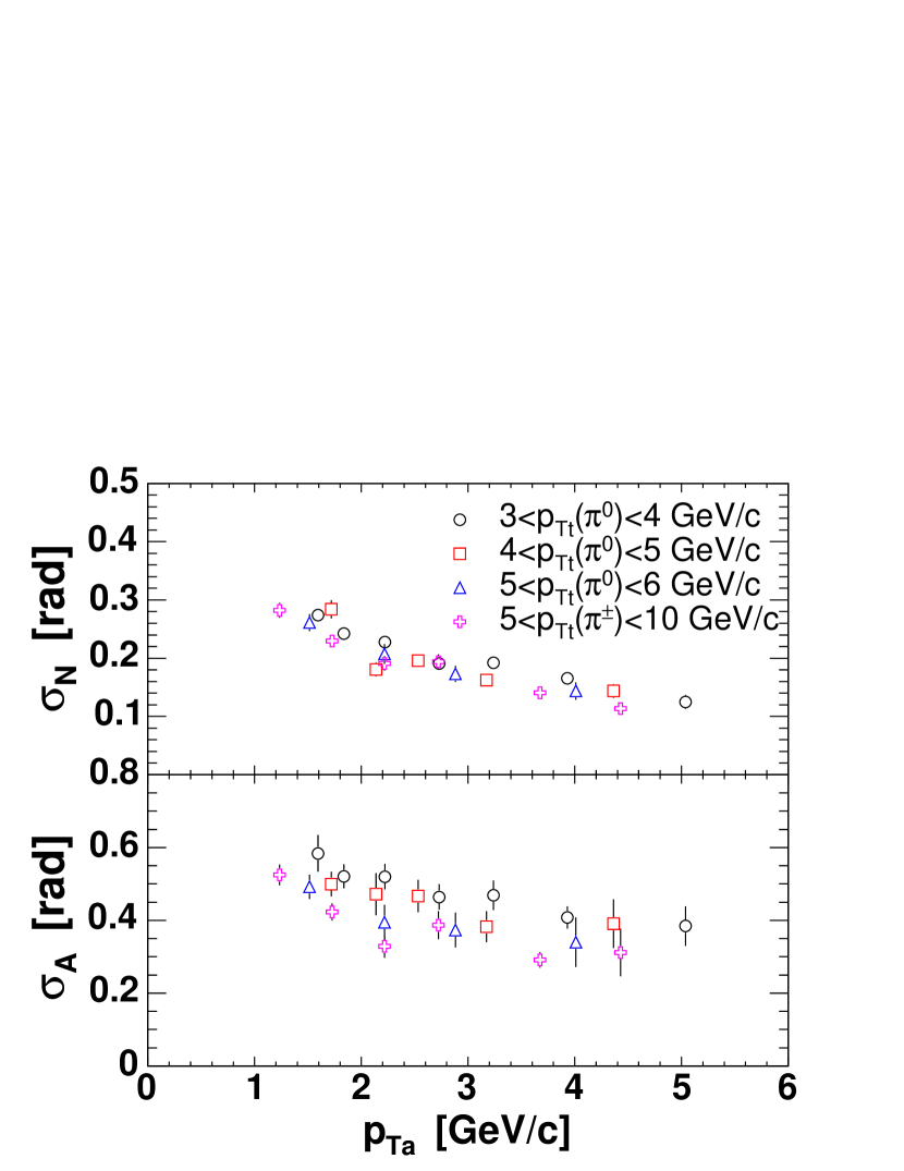
Figure 9: (color online) (top) The width of the near-side peak $\sigma_{\rm N}$ with $p_{T\rm a}$ for various values of $p_{T\rm t}$ as indicated in legend. (bottom) The width of the far-side peak $\sigma_{\rm A}$ with $p_{T\rm a}$ for the same $p_{T\rm t}$ selection.

The per-trigger yields as a function of $p_{T\rm t}$ for fixed associated $1.4<p_{T\rm a}<5.0$  GeV/$c$ bin are shown in Fig. 13. There is a distinct behavior of the near-side yield which varies with trigger $p_{T\rm t}$ much less than the away-side yield. For the away-side, this reflects the fact that the particle detected in the fixed associated bin are produced from the lower $z$ region of the fragmentation function for events with higher trigger $p_{T\rm t}$. For the near-side jet, this multiplicity increase is reduced due to the fact that with increasing $p_{T\rm t}$ the near-side jet energy increases; however, at the same time the larger fraction of this energy is taken away by the more energetic trigger particle. Thus the relative change in $z$ is smaller on the near-side.

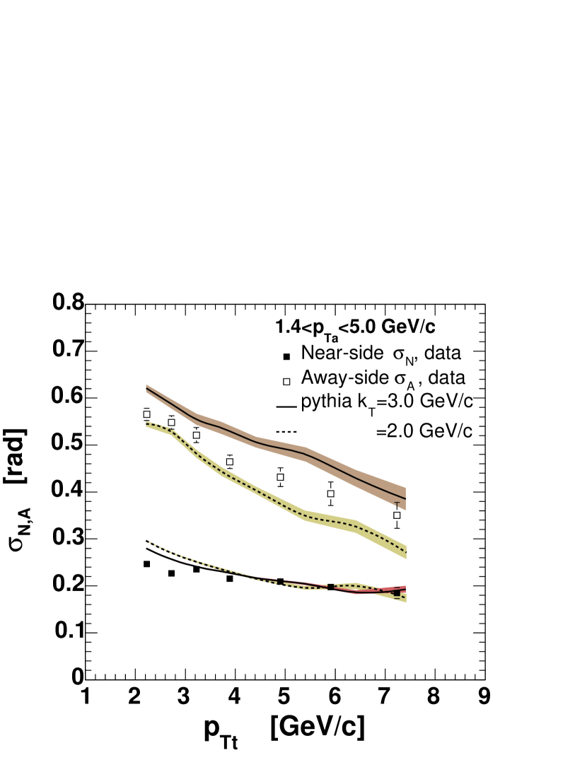
Figure 10: (color online) The near-side (squares) and away-side (circles) width as a function or trigger-$\pi^{0}$ $p_{T\rm t}$. The associated charged particle momenta are in the $1.4<p_{T\rm a}<5.0$  GeV/$c$ region. The curves are from a PYTHIA calculation with the values of $k_{T}$ indicated. The data values are given in Table 3.

Table 3: The $\sigma_{\rm N}$ and $\sigma_{\rm A}$ values shown in Fig. 10. All units in rad and  GeV/$c$. Only the statistical errors are shown.

$p_{T\rm t}$	$\sigma_{\rm N}$	$\sigma_{\rm A}$
2.23	0.247 $\pm$ 0.002	0.565 $\pm$ 0.013
2.72	0.227 $\pm$ 0.003	0.548 $\pm$ 0.014
3.22	0.235 $\pm$ 0.004	0.521 $\pm$ 0.016
3.89	0.215 $\pm$ 0.004	0.464 $\pm$ 0.014
4.90	0.210 $\pm$ 0.006	0.431 $\pm$ 0.020
5.91	0.197 $\pm$ 0.009	0.396 $\pm$ 0.025
7.23	0.185 $\pm$ 0.012	0.350 $\pm$ 0.028

In order to extract $\left<z_{\rm t}\right>$  and $\hat{x}_{\rm h}$ knowledge of the fragmentation function is needed; a detailed discussion is given in following sections.

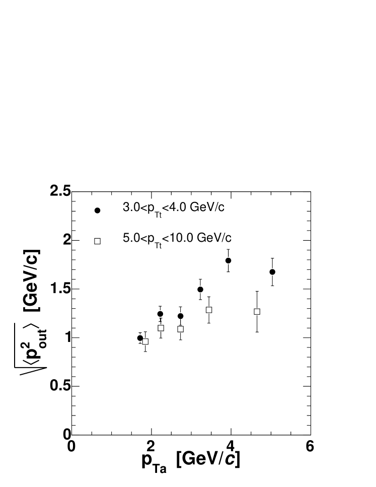
Figure 11: Extracted values of $\sqrt{\left<p_{\rm out}^{2}\right>}$ for $3.0<p_{T\rm t}<4.0$ and $5.0<p_{T\rm t}<10.0$  GeV/$c$ for various values of $p_{T\rm a}$ using the direct $p_{\rm out}$ extraction method based on fitting the away-side peak by Eq. (23).

Figure 12: (solid circles) Extracted values of $\sqrt{\left<p_{\rm out}^{2}\right>}$ for $1.4<p_{T\rm a}<5.0$  GeV/$c$ for various values of $p_{T\rm t}$ from Eq. (23). (open diamonds) Indirect $p_{\rm out}$=$p_{T\rm a}$sin($\sigma_{\rm A}$) values.

Table 4: The $\sqrt{\left<p_{\rm out}^{2}\right>}$ values shown in Fig. 11 and Fig. 12. All units in  GeV/$c$. Only the statistical errors are shown.

$1.4<p_{T\rm a}<5.0$		$3<p_{T\rm t}<4$		$5<p_{T\rm t}<10$
$p_{T\rm t}$	$\sqrt{\left<p_{\rm out}^{2}\right>}$	$p_{T\rm a}$	$\sqrt{\left<p_{\rm out}^{2}\right>}$	$p_{T\rm a}$	$\sqrt{\left<p_{\rm out}^{2}\right>}$
2.23	1.315 $\pm$ 0.043	1.72	0.996 $\pm$ 0.056	1.85	0.960 $\pm$ 0.102
2.72	1.250 $\pm$ 0.046	2.22	1.244 $\pm$ 0.079	2.24	1.100 $\pm$ 0.103
3.22	1.182 $\pm$ 0.049	2.73	1.222 $\pm$ 0.095	2.73	1.088 $\pm$ 0.110
3.89	1.011 $\pm$ 0.038	3.23	1.496 $\pm$ 0.105	3.44	1.285 $\pm$ 0.136
4.90	0.953 $\pm$ 0.052	3.93	1.793 $\pm$ 0.115	4.65	1.268 $\pm$ 0.210
5.91	0.868 $\pm$ 0.064	5.04	1.675 $\pm$ 0.141
7.24	0.798 $\pm$ 0.068

Table 5: The near and away side conditional yield per number of triggers for $1.4<p_{T\rm a}<5.0$  GeV/$c$ shown in Fig. 13. All units in rad and  GeV/$c$. Only the statistical errors are shown.

$p_{T\rm t}$	$Y_{N}$	$Y_{A}$
2.23	1.911 $\pm$ 0.018	1.717 $\pm$ 0.044
2.72	1.863 $\pm$ 0.022	1.908 $\pm$ 0.055
3.22	2.032 $\pm$ 0.032	2.130 $\pm$ 0.071
3.89	1.966 $\pm$ 0.033	2.360 $\pm$ 0.074
4.90	2.120 $\pm$ 0.061	2.611 $\pm$ 0.123
5.91	2.153 $\pm$ 0.098	2.992 $\pm$ 0.196
7.24	2.174 $\pm$ 0.125	3.690 $\pm$ 0.242

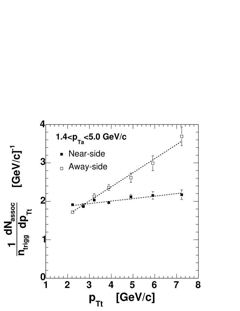
Figure 13: Measured yield of charged hadrons associated with one trigger $\pi^{0}$ with transverse momenta indicated in Table 1 and associated charged hadron with $1.4<p_{T\rm<}5.0\mbox{~{}GeV/$c$}$. Dashed lines represent the linear fit.

IV.1 $\sqrt{\left<j_{T\rm}^{2}\right>}$ and $\hat{x}_{\rm h}^{-1}\left<z_{\rm t}\right>\sqrt{\left<k_{T\rm}^{2}\right>}$ results

The measurement is performed in two different kinematical regimes; first the transverse momentum of the trigger particle, $p_{T\rm t}$, is fixed and the peak width is measured for different values of associated particle transverse momenta $p_{T\rm a}$ (Fig. 9). (Note that in the region of overlap, the data are in excellent agreement with a

Table 6: The $\sqrt{\left<j_{T\rm}^{2}\right>}$ values shown in Fig. 14 and Fig. 15. All units in rad and  GeV/$c$. Only the statistical errors are shown.

$1.4<p_{T\rm a}<5.0$		$3<p_{T\rm t}<4$
$p_{T\rm t}$	$\sqrt{\left<j_{T\rm}^{2}\right>}$	$p_{T\rm a}$	$\sqrt{\left<j_{T\rm}^{2}\right>}$
3.22	0.587 $\pm$ 0.009	1.72	0.562 $\pm$ 0.011
3.89	0.577 $\pm$ 0.009	2.22	0.597 $\pm$ 0.014
4.90	0.600 $\pm$ 0.017	2.73	0.572 $\pm$ 0.017
5.91	0.596 $\pm$ 0.026	3.23	0.590 $\pm$ 0.020
7.24	0.597 $\pm$ 0.038	3.93	0.603 $\pm$ 0.017
8.34	0.632 $\pm$ 0.085	5.04	0.506 $\pm$ 0.029
$4<p_{T\rm t}<5$		$5<p_{T\rm t}<6$
$p_{T\rm a}$	$\sqrt{\left<j_{T\rm}^{2}\right>}$	$p_{T\rm a}$	$\sqrt{\left<j_{T\rm}^{2}\right>}$
1.72	0.643 $\pm$ 0.036	1.52	0.529 $\pm$ 0.030
2.14	0.492 $\pm$ 0.032	2.22	0.581 $\pm$ 0.049
2.53	0.608 $\pm$ 0.035	2.88	0.590 $\pm$ 0.047
3.17	0.590 $\pm$ 0.032	4.01	0.603 $\pm$ 0.063
4.36	0.631 $\pm$ 0.052

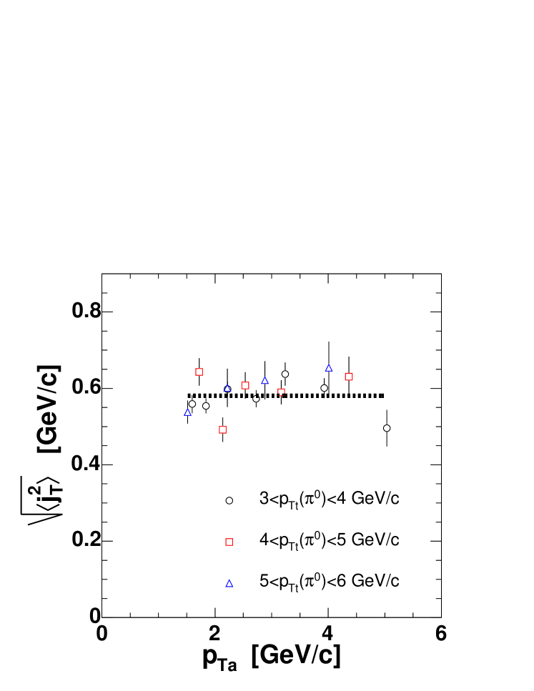
Figure 14: (color online) $\left<j_{T\rm}^{2}\right>$ values calculated according Eq. (16). The dashed line represents the 0^th-order polynomial fit in the $1.5<p_{T\rm a}<5$  GeV/$c$ region.

Figure 15: Averaged values of $\left<j_{T\rm}^{2}\right>$ in (1.5$<p_{T\rm a}<$5  GeV/$c$) as a function of the trigger transverse momentum $p_{T\rm t}$ (solid triangles). The CCOR values measured at $\sqrt{s}$=62.4  GeV shown by open triangles.

previous measurement Adams et al. (2003).) In the second case, particle pairs with a fixed associated bin $1.4<p_{T\rm a}<5.0$  GeV/$c$ and various $p_{T\rm t}$ are selected (Fig. 10). It is evident that both near and away-side correlation peaks in all cases reveal a decreasing trend with $p_{T\rm a}$ and $p_{T\rm t}$.

However, the asymptotic behavior of $\sigma_{\rm N}$ and $\sigma_{\rm A}$ is different. Whereas the magnitude of $\sigma_{\rm N}$, according to Eq. (16), should vanish for large values of $p_{T\rm t}$ and $p_{T\rm a}$, the $\sigma_{\rm A}$  according to Eq. (22) should be approximately constant around $\hat{x}_{\rm h}^{-1}\left<z_{\rm t}\right>\sqrt{\left<k_{T\rm}^{2}\right>}$/$p_{T\rm t}$ for large values of $p_{T\rm a}$. The $\left<z_{\rm t}\right>$ and $\hat{x}_{\rm h}$ quantities are implicitly $p_{T\rm a}$ dependent, however, their ratio is roughly $\sim 1$ so that the asymptotic value of $\sigma_{\rm A}$$\big{|}_{p_{T\rm a}\rightarrow\infty}\sim$$\sqrt{\left<k_{T\rm}^{2}\right>}$/$p_{T\rm t}$.

Extracted values of $\left<j_{T\rm}^{2}\right>$ as a function of $p_{T\rm a}$ according to Eq. (16) are shown in Fig. 14. All $\left<j_{T\rm}^{2}\right>$ values are constant in the explored region ($p_{T\rm a}$$>$1.5  GeV/$c$). It is expected that $\left<j_{T\rm}^{2}\right>$ can not remain constant for arbitrarily small values of $p_{T\rm a}$ because of the phase space limitation. In the region where $p_{T\rm a}$$\leq$$\sqrt{\left<j_{T\rm}^{2}\right>}$, the magnitude of the $j_{T\rm}$-vector is truncated, similar to the “Seagull effect” van Apeldoorn et al. (1975). Since the $\sqrt{\left<j_{T\rm}^{2}\right>}$ values are on the order of 600  MeV/$c$, we assume that the phase space limitation can be safely neglected for $p_{T\rm a}$$>$1.5  GeV/$c$ and we extract the values of $\sqrt{\left<j_{T\rm}^{2}\right>}$ averaged over $p_{T\rm a}$ and $p_{T\rm t}$ (see Fig. 15)

$$\sqrt{\left<j_{T\rm}^{2}\right>}=585\pm 6(\rm stat)\pm 15(\rm sys)\mbox{~{}MeV/$c$}$$ (24)

The systematic error originates from the finite momentum resolution and Eq. (16) where we assume that the arc-sine function can be approximated by its argument. For the angular width of the near angle peak (see Fig. 9 and Fig. 10) it corresponds to an uncertainty of order of 3%.

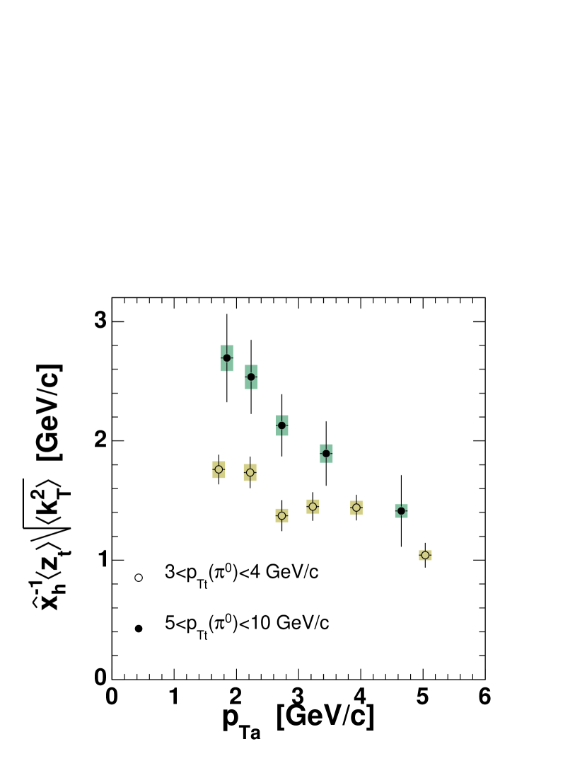
Figure 16: (color online) $\hat{x}_{\rm h}$^-1$\left<z_{\rm t}\right>\sqrt{\left<k_{T\rm}^{2}\right>}$ values calculated according to Eq. (22) for trigger $\pi^{0}$ in $3<p_{T\rm t}<4$  GeV/$c$ and $5<p_{T\rm t}<6$  GeV/$c$ as a function of $p_{T\rm a}$. The systematic uncertainties are indicated by the shaded boxes.

The independence of $\left<j_{T\rm}^{2}\right>$ on either $p_{T\rm t}$ or $\sqrt{s}$ has been observed by the CCOR experiment in the range $\sqrt{s}$=31–62.4  GeV Angelis et al. (1980). The $\left<j_{T\rm}^{2}\right>$ values at $\sqrt{s}$=62.4  GeV (open triangles on Fig. 15) are systematically larger then values found in this analysis. The discrepancy should not be taken as significant, as CCOR used a slightly different technique than in this paper. CCOR extracted the $\left<j_{T\rm}^{2}\right>$ values from measurements of $\left<|p_{\rm out}|\right>$ for different values of the $x_{E}$ variable Eq. (19). According to Eq. (18) the $\left<|p_{\rm out}|\right>$² magnitude should depend linearly on $x^{2}_{E}$; and the $\left<|j_{T\rm y}|\right>$ value was extracted from the intercept of the $\left<p_{\rm out}\right>$${}^{2}(x_{E}$) fit at $x_{E}$=0, rather than from a measurement of $\sigma_{\rm N}$.

Knowing the $\left<j_{T\rm}^{2}\right>$ and $p_{\rm out}$ values, we used Eq. (22) to determine $\hat{x}_{\rm h}^{-1}\left<z_{\rm t}\right>\sqrt{\left<k_{T\rm}^{2}\right>}$ (see Fig. 16 and Fig. 17). The systematic error was estimated with Monte Carlo simulations to be on the order of 5%. The main source of systematic error originates from the assumption (Eqs. (16) and (21)) of the relative smallness of $\left<j_{T\rm}^{2}\right>$, collinearity between $p_{\rm out}$ and $j_{T\rm ay}$ and from the limited momentum resolution discussed in section III.

Figure 17: (color online) The same calculation according Eq. (22) for fixed associated bin $1.4<p_{T\rm a}<5.0$  GeV/$c$ as a function of $p_{T\rm t}$. The systematic errors indicated by colored rectangles. The $\sqrt{\left<k_{T\rm}^{2}\right>}$ results obtained by CCOR collaboration at $\sqrt{s}$=62.4  GeV Angelis et al. (1980) displayed by solid triangles.

The $p_{T\rm a}$ dependence of the extracted $\hat{x}_{\rm h}^{-1}\left<z_{\rm t}\right>\sqrt{\left<k_{T\rm}^{2}\right>}$ (Fig. 16) reveals a strikingly decreasing trend. It was originally expected that by fixing the value of $p_{T\rm t}$, the kinematics of the hard scattering (i.e. $\hat{p}_{T\rm t}$$\simeq$$\hat{p}_{T\rm a}$) would be fixed, independently of the value of $p_{T\rm a}$. Various values of $p_{T\rm a}$ would then sample the $\hat{p}_{T\rm a}$ fragmentation function, and the value of $\hat{x}_{\rm h}^{-1}\left<z_{\rm t}\right>\sqrt{\left<k_{T\rm}^{2}\right>}$ was expected to be constant. It is evident that this assumption is not quite correct.

A similar line of argument applies also for the rising trend when $p_{T\rm a}$ is fixed and $p_{T\rm t}$ varies (Fig. 17). It is interesting to note that the CCOR $\sqrt{\left<k_{T\rm}^{2}\right>}$ values measured at $\sqrt{s}$=62.4  GeV (open triangles on Fig. 17) reveal a similar rising trend. However, the rising trend of $\hat{x}_{\rm h}^{-1}\left<z_{\rm t}\right>\sqrt{\left<k_{T\rm}^{2}\right>}$ with $p_{T\rm t}$ and falling with $p_{T\rm a}$ suggests that the variation of $\sqrt{\left<k_{T\rm}^{2}\right>}$ with $p_{T\rm t}$ seen by the CCOR collaboration Angelis et al. (1980) may be indicative of the $\langle z_{t}\rangle\hat{x}_{h}^{-1}$ variation which was there neglected. In order to understand variation of $\left<z_{\rm t}\right>$ and $\hat{x}_{\rm h}$ we have to explore the process of dijet fragmentation.

V Fragmentation Functions

We have shown in Eq. (22) that the width of the away side correlation peak

is related to the product of $\hat{x}_{\rm h}^{-1}\left<z_{\rm t}\right>\sqrt{\left<k_{T\rm}^{2}\right>}$. In order to evaluate $\left<z_{\rm t}\right>$, knowledge of the scattered parton $\hat{p}_{T}$ spectrum and fragmentation function is required.

Fragmentation functions from $e^{+}e^{-}$ collisions, weighted by the appropriate hard-scattering constituent cross-sections and $Q^{2}$ evolution could in principle be used. However, it was originally thought that the shape of the fragmentation function could be deduced from present measurements using the combined analysis of the inclusive trigger $p_{T\rm t}$ and associated particle $p_{T\rm a}$ distributions. Although this idea turned out to be incorrect, we will follow this line of reasoning for a while as it is instructive.

Generally, the invariant cross section for inclusive hadron production from jets can be parametrized in the following way. First, we assume that the number of parton fragments (consider only pions for simplicity) at a given $p_{T\rm}$ corresponds to the sum over all contributions from parton momenta, $\hat{p}_{T\rm}$  from $p_{T}<\hat{p}_{T\rm}<\sqrt{s}/2$. The joint probability of detecting a pion with $p_{T\rm}$$=z\hat{p}_{T\rm}$ originating from a parton with $\hat{p}_{T\rm}$ can be written as

$${d^{2}\sigma_{\pi}\over\hat{p}_{T\rm}d\hat{p}_{T\rm}dz} = {d\sigma_{q}\over\hat{p}_{T\rm}d\hat{p}_{T\rm}}\times D^{q}_{\pi}(z)$$ (25)

$$= f_{q}(\hat{p}_{T})\times D^{q}_{\pi}(z).$$

Here we use $f_{q}(\hat{p}_{T})$ to represent the final state scattered-parton invariant spectrum $d\sigma_{q}/\hat{p}_{T\rm}d\hat{p}_{T\rm}$ and $D^{q}_{\pi}(z)$ to represent the fragmentation function. The first term in Eq. (25) can be viewed as a probability of finding a parton with transverse momentum $\hat{p}_{T\rm}$ and the second term corresponds to the probability that the parton fragments into a particle of momentum $p_{T\rm}$$=z\hat{p}_{T\rm}$. With a simple change of variables from $\hat{p}_{T\rm}$ to $p_{T\rm}$$=z\hat{p}_{T\rm}$, we obtain the joint probability of a pion with $p_{T\rm}$ which is a fragment with momentum fraction $z$ from a parton with $\hat{p}_{T\rm}$=$p_{T\rm}$$/z$:

$${d^{2}\sigma_{\pi}\over p_{T\rm}dp_{T\rm}dz}=f_{q}({p_{T}\over z})\cdot D^{q}_{\pi}(z)\;{1\over z^{2}}.$$ (26)

The $p_{T\rm}$ and $z$ dependences do not factorize. However, the $p_{T\rm}$ spectrum may be found by integrating over all values of $\hat{p}_{T\rm}$ $\geq$ $p_{T\rm}$ to $\hat{p}_{T\rm}$${}_{max}=\sqrt{s}/2$, which corresponds to values of $z$ from $x_{T}=2p_{T}/\sqrt{s}$ to 1.

$${1\over p_{T\rm}}{d\sigma_{\pi}\over dp_{T\rm}}=\int_{x_{T}}^{1}f_{q}({p_{T}\over z})\cdot D^{q}_{\pi}(z)\;{dz\over z^{2}}$$ (27)

Alternatively, for any fixed value of $p_{T\rm}$ one can evaluate the $\left<z(p_{T})\right>$, integrated over the parton spectrum:

$$\left<z(p_{T})\right>={{\int_{x_{T}}^{1}z\;D^{q}_{\pi}(z)\;f_{q}(\hat{p}_{T})\ (p_{T\rm}/z){dz\over z^{2}}}\over{\int_{x_{T}}^{1}D^{q}_{\pi}(z)\;f_{q}(p_{T\rm}/z){dz\over z^{2}}}}\qquad.$$ (28)

From the scaling properties of QCD and from the shape of the $\pi^{0}$ invariant cross section itself, which is a pure power law for $p_{T}\geq 3$ GeV/c Adler et al. (2003e), one can deduce that $f_{q}(\hat{p}_{T})$ should have a power law shape, $f_{q}(\hat{p}_{T})=A\hat{p}_{T\rm}^{-n}$. In this case the hadron spectrum also has a power law shape because

$${1\over p_{T\rm}}{d\sigma_{\pi}\over dp_{T\rm}} \approx \int_{x_{T}}^{1}A\,D^{q}_{\pi}(z)\cdot({p_{T}\over z})^{-n}{dz\over z^{2}}$$ (29)

$$\approx {A\over{p_{T\rm}^{n}}}\int_{x_{T}}^{1}\,D^{q}_{\pi}(z)\cdot{z}^{n-2}dz$$

and the last integral depends only weakly on $p_{T\rm}$ due to the small value of $x_{T}$. For small parton $\hat{p}_{T\rm}$ (below 3-4  GeV/$c$) the power law shape is no longer valid, but the region $p_{T}<3$ GeV/c is outside the scope of this paper. The $f_{q}(\hat{p}_{T})$ should also diminish for very high $\hat{p}_{T\rm}$$\rightarrow\sqrt{s}/2$ where the phase space available for hard parton production diminishes, again not relevant for the present purposes.

We used the power law parameterization for the final state scattered-parton invariant spectrum $f_{q}(\hat{p}_{T})\propto\hat{p}_{T\rm}^{-n}$ where $n$ is a free parameter which can be determined from the fit of Eq. (27) to the measured $\pi^{0}$ cross section. There is, however, one more missing piece of information - the shape of the fragmentation function $D^{q}_{\pi}$. In an attempt to extract this information from the data, we have analyzed associated $x_{E}$-distributions, as shown in Table 7.

Table 7: Measured $x_{E}$ distributions associated with various transverse momenta of the trigger $\pi^{0}$. Only the statistical errors are shown.

$p_{T\rm t}$=3.39  GeV/$c$		$p_{T\rm t}$=4.40  GeV/$c$		$p_{T\rm t}$=5.41  GeV/$c$		$p_{T\rm t}$=6.40  GeV/$c$		$p_{T\rm t}$=7.39  GeV/$c$
$x_{E}$	$dn/dx_{E}$	$x_{E}$	$dn/dx_{E}$	$x_{E}$	$dn/dx_{E}$	$x_{E}$	$dn/dx_{E}$	$x_{E}$	$dn/dx_{E}$
0.32	2.7e+00 $\pm$ 4.7e-02	0.23	6.7e-01 $\pm$ 2.2e-02	0.22	2.3e-01 $\pm$ 1.2e-02	0.18	8.0e-02 $\pm$ 6.3e-03	0.17	1.8e-02 $\pm$ 3.1e-03
0.37	1.9e+00 $\pm$ 4.0e-02	0.27	6.8e-01 $\pm$ 2.2e-02	0.27	1.4e-01 $\pm$ 9.6e-03	0.22	4.6e-02 $\pm$ 4.7e-03	0.24	9.0e-03 $\pm$ 1.5e-03
0.42	1.4e+00 $\pm$ 3.3e-02	0.32	4.8e-01 $\pm$ 1.9e-02	0.32	9.4e-02 $\pm$ 7.7e-03	0.27	3.1e-02 $\pm$ 3.9e-03	0.33	4.4e-03 $\pm$ 1.0e-03
0.47	9.6e-01 $\pm$ 2.8e-02	0.37	2.9e-01 $\pm$ 1.4e-02	0.37	5.7e-02 $\pm$ 6.0e-03	0.35	1.7e-02 $\pm$ 2.0e-03	0.45	2.8e-03 $\pm$ 8.1e-04
0.52	7.3e-01 $\pm$ 2.4e-02	0.42	2.2e-01 $\pm$ 1.2e-02	0.43	4.1e-02 $\pm$ 5.0e-03	0.44	8.2e-03 $\pm$ 1.4e-03	0.55	6.9e-04 $\pm$ 4.0e-04
0.57	5.2e-01 $\pm$ 2.0e-02	0.47	1.5e-01 $\pm$ 1.0e-02	0.47	2.8e-02 $\pm$ 4.2e-03	0.54	3.8e-03 $\pm$ 9.2e-04	0.64	4.5e-04 $\pm$ 3.2e-04
0.62	3.8e-01 $\pm$ 1.7e-02	0.52	8.0e-02 $\pm$ 7.4e-03	0.52	2.3e-02 $\pm$ 3.8e-03	0.64	2.4e-03 $\pm$ 7.3e-04
0.67	3.0e-01 $\pm$ 1.5e-02	0.57	8.6e-02 $\pm$ 7.7e-03	0.57	1.9e-02 $\pm$ 3.4e-03	0.81	9.3e-04 $\pm$ 2.6e-04
0.75	2.1e-01 $\pm$ 9.0e-03	0.62	5.8e-02 $\pm$ 6.3e-03	0.63	1.1e-02 $\pm$ 2.5e-03
0.85	1.1e-01 $\pm$ 6.5e-03	0.68	4.9e-02 $\pm$ 5.7e-03	0.67	1.1e-02 $\pm$ 2.5e-03
0.95	8.2e-02 $\pm$ 5.5e-03	0.75	3.2e-02 $\pm$ 3.3e-03	0.76	5.6e-03 $\pm$ 1.3e-03
1.04	5.4e-02 $\pm$ 4.5e-03	0.85	2.0e-02 $\pm$ 2.5e-03	0.85	2.9e-03 $\pm$ 9.2e-04
1.15	3.6e-02 $\pm$ 3.6e-03	0.94	1.6e-02 $\pm$ 2.2e-03	0.97	2.3e-03 $\pm$ 8.1e-04
1.25	2.8e-02 $\pm$ 3.2e-03	1.04	7.0e-03 $\pm$ 1.5e-03	1.07	8.3e-04 $\pm$ 4.8e-04

V.1 ’Scaling’ variable $x_{\rm E}$

It was expected Darriulat et al. (1976) that the $x_{\rm E}$ variable, defined by Eq. (19), to first order, approximates the fragmentation function in the limit of high values of $p_{T\rm t}$, where there is sufficient collinearity between the trigger particle and the fragmenting parton. In this case where $j_{T\rm}$$\ll$$p_{T\rm t}$ and $k_{T\rm}$$\ll$$p_{T\rm t}$ one can assume that $p_{T\rm t}$=$\hat{p}_{T\rm t}$/$z_{\rm t}$ and $x_{\rm E}\,z_{\rm t}=\hat{x}_{\rm h}\,p_{T\rm a}\,\cos{\Delta\phi}/\hat{p}_{T\rm a}\simeq\hat{x}_{\rm h}\,z_{\rm a}$, and thus the slopes of $D(z_{\rm a})$ and $x_{\rm E}$ are related as

$$\left<z_{\rm a}\right>\approx\left<x_{\rm E}\right>\left<z_{\rm t}\right>\hat{x}_{\rm h}^{-1}\qquad.$$ (30)

The $x_{\rm E}$ distributions of particles associated with trigger particles in the 3-8  GeV/$c$ range of transverse momentum are plotted in Fig. 18. The dashed lines represent exponential fits. The slopes of these exponentials range from $-5.8$ ($3<p_{T\rm t}<4$  GeV/$c$) to $-7.8$ (open symbols on Fig. 19). This is qualitatively and quantitatively different from the similar measurement done by CCOR collaboration at $\sqrt{s}$=62.4  GeV where the slopes of exponential fits to the $x_{\rm E}$ distributions were found to be $\approx-5.3$ and independent of the trigger transverse momenta. That observation also supported the hypothesis of the $x_{\rm E}$ distribution being a good approximation of the fragmentation function. We also note that the $x_{\rm E}$ distributions are not quite exponential and at large values of $x_{\rm E}$ there is a tail similar to the power law tail of the single inclusive $p_{T\rm}$ distribution.

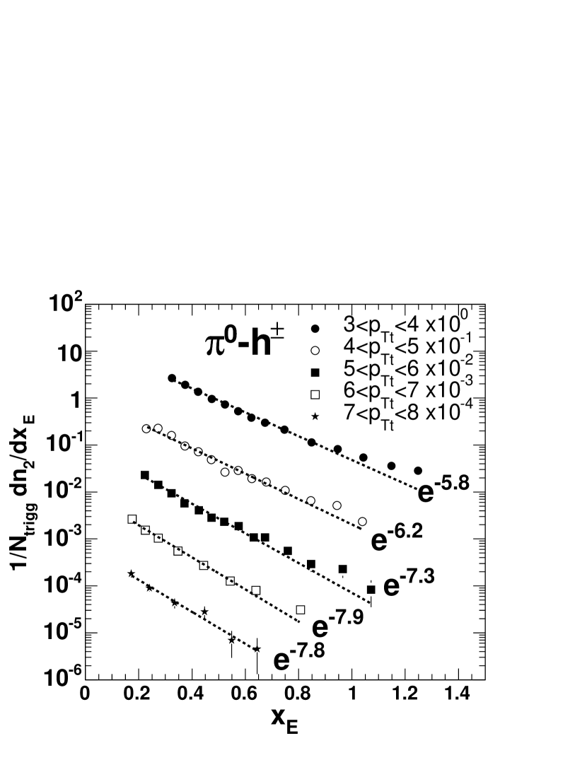
Figure 18: The distribution of associated particles with $x_{\rm E}$ variable for various trigger particle $p_{T\rm t}$ indicated in the legend. Exponential fits indicated by dashed lines.

The reason why the $x_{\rm E}$ distributions do not have the same slope for different $p_{T\rm t}$ and why there is a “power law” tail at large $x_{\rm E}$ is the same as that which causes $\hat{x}_{\rm h}^{-1}\left<z_{\rm t}\right>\sqrt{\left<k_{T\rm}^{2}\right>}$ to decrease with the associated particle transverse momentum. It turns out that by sampling different regions of $p_{T\rm a}$ for fixed $p_{T\rm t}$, the average momentum of the parton fragmenting into a trigger particle, $\left<z_{\rm t}\right>$, also changes. This kind of trigger bias causes the hard scattering kinematics, the value of $\hat{p}_{T}$, to not be fixed for the case where $p_{T\rm t}$ is fixed but $p_{T\rm a}$ varies.

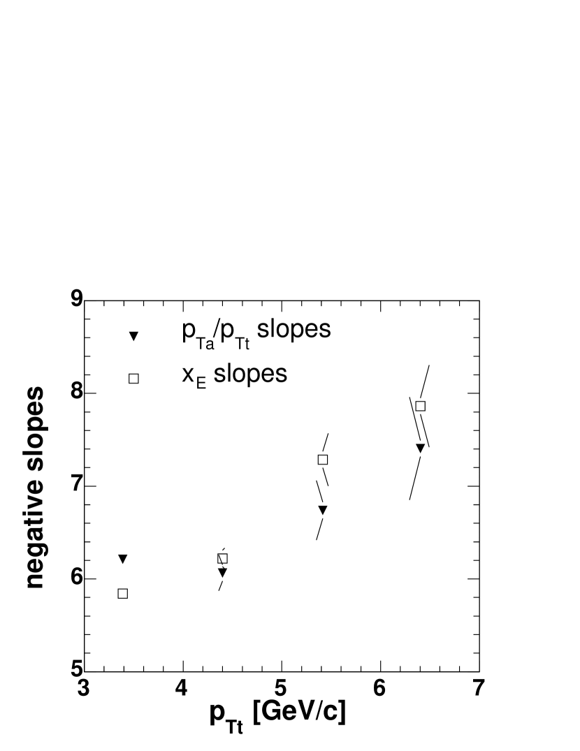
Figure 19: The negative slope parameters extracted from the fit of a plain exponential function into a $x_{\rm E}$ (see Fig. 18) and $p_{T\rm a}$/$p_{T\rm t}$ (see Fig. 20) distributions.

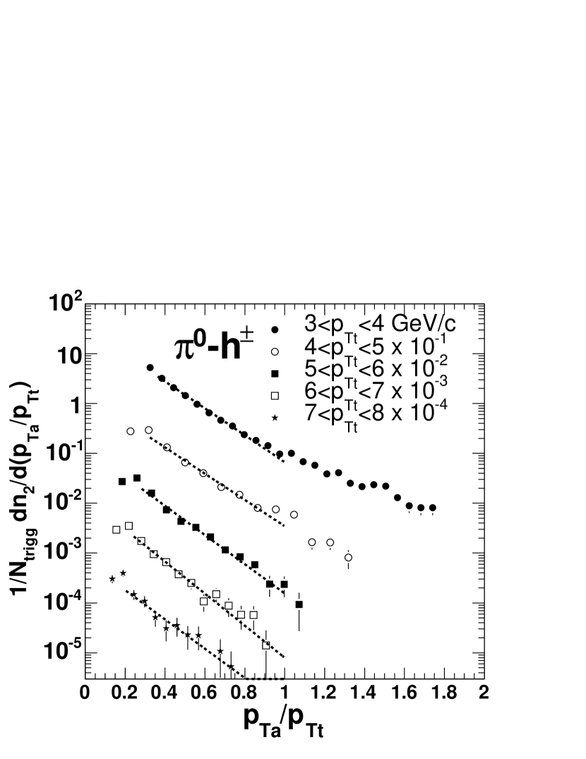
Figure 20: The distribution of associated particles with $p_{T\rm a}$/$p_{T\rm t}$ variable for various trigger particle $p_{T\rm t}$ indicated in the legend. The distribution were fitted in the limited range $0.2<p_{T\rm a}/p_{T\rm t}<0.4$ by an exponential function (dashed lines).

Taking this into account, one can not treat the associated $x_{\rm E}$ distribution as a rescaled fragmentation function, but rather as a folding of the two fragmentation processes of trigger and associated jets. The same line of arguments applies also for other two-particle variables, e.g.$p_{T\rm a}$/$p_{T\rm t}$, Wang (2004) used for an approximation of the fragmentation variable $z$ (see Fig. 20). The negative slopes of an exponential fit in the $0.2<p_{T\rm a}/p_{T\rm t}<0.4$ range (solid symbols on Fig. 19) are, within the error bars, the same as for $x_{\rm E}$.

In conclusion: the slope parameters extracted from associated $x_{\rm E}$ distributions reveal the rising trend with $p_{T\rm t}$ which reflects the fact, that the different $p_{T\rm a}$ samples not only different $z_{\rm a}$ but also different $z_{\rm t}$.

The description of an associated distribution detected under the condition of the existence of a trigger particle requires an extension of the formulae discussed in V and is a subject of the next section.

VI Dijet fragmentation

For the description of the detection of a single particle which is the result of jet fragmentation, recall Eq. (25)

$${d^{2}\sigma_{\pi}\over d\hat{p}_{T\rm}dz_{\rm t}} = {d\sigma_{q}\over d\hat{p}_{T\rm}}\times D^{q}_{\pi}(z_{\rm t})$$

$$= \hat{p}_{T\rm}f_{q}(\hat{p}_{T})\times D^{q}_{\pi}(z_{\rm t})\equiv\Sigma_{q}(\hat{p}_{T})\times D^{q}_{\pi}(z_{\rm t})$$

where we have now explicitly labeled the $z$ of the trigger particle as $z_{\rm t}$, and defined

$$\Sigma_{q}(\hat{p}_{T})\equiv\hat{p}_{T\rm}\;f_{q}(\hat{p}_{T})={d\sigma_{q}\over d\hat{p}_{T\rm}}\qquad.$$ (32)

When $k_{T\rm}$ smearing is introduced, configurations for which the high $p_{T\rm}$ parton pair is on the average moving towards the trigger particle are favored due to the steeply falling $\hat{p}_{T\rm}$ spectrum, such that:

$$\left<\hat{p}_{T\rm t}-\hat{p}_{T\rm}\right>\simeq{1\over 2}\left<\hat{p}_{T\rm t}-\hat{p}_{T\rm a}\right>\equiv s(k_{T\rm})$$

with small variance $\sigma^{2}_{s}$, and we explicitly introduced $\hat{p}_{T\rm t}$ and $\hat{p}_{T\rm a}$ to represent the transverse momenta of the trigger and away partons. The single inclusive $p_{T\rm t}$ spectrum is now given by

$${d^{2}\sigma_{\pi}\over d\hat{p}_{T\rm t}dz_{\rm t}}=\Sigma^{\prime}_{q}(\hat{p}_{T\rm t})\times D^{q}_{\pi}(z_{\rm t})$$ (33)

where the trigger parton $\hat{p}_{T\rm t}$ spectrum after $k_{T\rm}$ smearing is

$$\Sigma^{\prime}_{q}(\hat{p}_{T\rm t})\equiv\hat{p}_{T\rm t}\;f^{\prime}_{q}(\hat{p}_{T\rm t})={d\sigma_{q}\over d\hat{p}_{T\rm t}}\qquad.$$ (34)

Then, the conditional probability for finding the away side parton with $\hat{p}_{T\rm a}$ and $z_{\rm a}$, given $\hat{p}_{T\rm t}$ (and $z_{\rm t}$), is:

$$\left.{dP(\hat{p}_{T\rm a},z_{\rm a})\over d\hat{p}_{T\rm a}dz_{\rm a}}\right|_{\hat{p}_{T\rm t}}=C(\hat{p}_{T\rm a},\hat{p}_{T\rm t},k_{T\rm})D^{q}_{\pi}(z_{\rm a})$$

where $C(\hat{p}_{T\rm a},\hat{p}_{T\rm t},k_{T\rm})$ represents the distribution of the transverse momentum of the away parton $\hat{p}_{T\rm a}$, given $\hat{p}_{T\rm t}$ and $k_{T\rm}$, which can be written as:

$$C(\hat{p}_{T\rm a},\hat{p}_{T\rm t},k_{T\rm})=$$ (35)

$$={1\over\sqrt{2\pi\sigma^{2}_{s}}}\,\exp\left(-[\hat{p}_{T\rm a}-(\hat{p}_{T\rm t}-2s(k_{T\rm}))]^{2}\over{2\sigma^{2}_{s}}\right)$$                                                           .

Then

$${d^{4}\sigma_{\pi}\over d\hat{p}_{T\rm t}dz_{\rm t}d\hat{p}_{T\rm a}dz_{\rm a}}={d^{2}\sigma_{\pi}\over d\hat{p}_{T\rm t}dz_{\rm t}}\times\left.{dP(\hat{p}_{T\rm a},z_{\rm a})\over d\hat{p}_{T\rm a}dz_{\rm a}}\right|_{\hat{p}_{T\rm t}}\qquad.$$

In general, $\sigma_{s}/s(k_{T\rm})$ is small (see section VI.2) so that $C(\hat{p}_{T\rm a},\hat{p}_{T\rm t},k_{T\rm})$ is well approximated by a $\delta$ function and we may take

$$\hat{p}_{T\rm a}=\hat{p}_{T\rm t}-2s(k_{T\rm})=\hat{x}_{\rm h}\hat{p}_{T\rm t}\qquad,$$

so that

$${d^{3}\sigma_{\pi}\over d\hat{p}_{T\rm t}dz_{\rm t}dz_{\rm a}}=\Sigma^{\prime}_{q}(\hat{p}_{T\rm t})D^{q}_{\pi}(z_{\rm t})D^{q}_{\pi}(z_{\rm a})$$

where

$$z_{\rm a}={p_{T\rm a}\over\hat{p}_{T\rm a}}={p_{T\rm a}\over\hat{x}_{\rm h}\hat{p}_{T\rm t}}={z_{\rm t}p_{T\rm a}\over\hat{x}_{\rm h}p_{T\rm t}}\qquad.$$

Changing variables from $\hat{p}_{T\rm t},z_{\rm t}$ to $p_{T\rm t},z_{\rm t}$ as above, and similarly from $z_{\rm a}$ to $p_{T\rm a}$, we obtain

$${d^{3}\sigma_{\pi}\over dp_{T\rm t}dz_{\rm t}dp_{T\rm a}}={1\over\hat{x}_{\rm h}p_{T\rm t}}\Sigma^{\prime}_{q}({p_{T\rm t}\over z_{\rm t}})D^{q}_{\pi}(z_{\rm t})D^{q}_{\pi}({z_{\rm t}p_{T\rm a}\over\hat{x}_{\rm h}p_{T\rm t}})$$ (36)

where for integrating over $z_{\rm t}$ or finding $\left<z_{\rm t}\right>$ for fixed $p_{T\rm t}$, $p_{T\rm a}$, the minimum value of $z_{\rm t}$ is $z_{\rm t}^{\rm min}=2p_{T\rm t}/\sqrt{s}=x_{Tt}$ and the maximum value is:

$$z_{\rm t}^{\rm max}=\hat{x}_{\rm h}{p_{T\rm t}\over p_{T\rm a}}={\hat{x}_{\rm h}\over x_{\rm h}}\qquad,$$

where $\hat{x}_{\rm h}(p_{T\rm t},p_{T\rm a})$ is also a function of $k_{T}$ (Eq. (20)).

Thus, in order to evaluate $\hat{x}_{\rm h}(p_{T\rm t},p_{T\rm a})$ for use in Eq. (36), $k_{T}$ must be known. We attack this problem by successive approximations. First we solve for $k_{T}$ and $D^{q}_{\pi}$(z) assuming $\hat{x}_{h}=1$ as done at the ISR where the smearing correction was small. Then we solve for $\hat{x}_{\rm h}(p_{T\rm t},p_{T\rm a})$ with this value of $k_{T}$ and iterate. On the first solution we solve only for $\Sigma^{\prime}_{q}(\hat{p}_{T\rm t})$ while on the iteration we include the $k_{T}$ smearing to solve for the unsmeared parton spectrum $\Sigma_{q}(\hat{p}_{T})$$=\hat{p}_{T\rm}\;f_{q}(\hat{p}_{T})$ (Eq. (32)).

VI.1 Sensitivity of the associated spectra to the fragmentation function

As discussed in section V.1, the associated $x_{E}$ distribution was thought to approximate the fragmentation function of the away jet. Equation 36 can be transformed to the $x_{E}$ distribution at fixed $p_{T\rm t}$ with a change of variables from $p_{T\rm a}$ to $x_{E}$ followed by integration over $z_{\rm t}$:

$${d^{2}\sigma\over dp_{T\rm t}dx_{\rm E}}={dp_{T\rm a}\over dx_{\rm E}}\times{d^{2}\sigma\over dp_{T\rm t}dp_{T\rm a}}\simeq\mbox{\hskip 72.26999pt}$$ (37)

$${1\over\hat{x}_{\rm h}}\int_{x_{T\rm t}}^{\hat{x}_{\rm h}{p_{T\rm t}\over p_{T\rm a}}}D^{q}_{\pi}(z_{\rm t})D^{q}_{\pi}({z_{\rm t}p_{T\rm a}\over\hat{x}_{\rm h}p_{T\rm t}})\Sigma^{\prime}_{q}({p_{T\rm t}\over z_{\rm t}})\,dz_{\rm t}.$$

We at first attempted to solve for the fragmentation function by simultaneous fits of the measured $x_{E}$ distributions to Eq. (37) constrained by a fit of the inclusive invariant $\pi^{0}$ cross section to Eq. (27). There were difficulties with convergence.

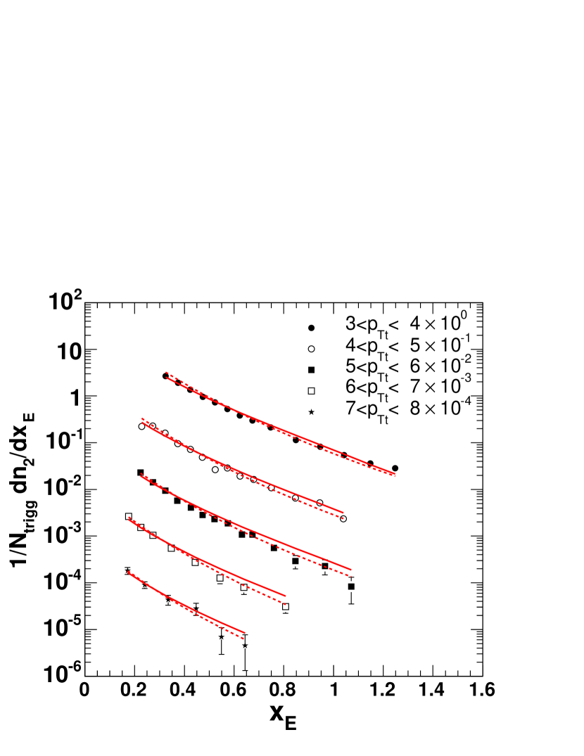
Figure 21: (color online) The same $x_{\rm E}$ distributions as on Fig. 18 shown with calculations according to Eq. (37) for quark (solid lines) and for gluon (dashed lines) $D(z)$. An exponential approximation was used and the slopes for quark and gluon fragmentation function were obtained by fitting to LEP data Abreu et al. (2000) and Alexander et al. (1996) (see Fig. 22).

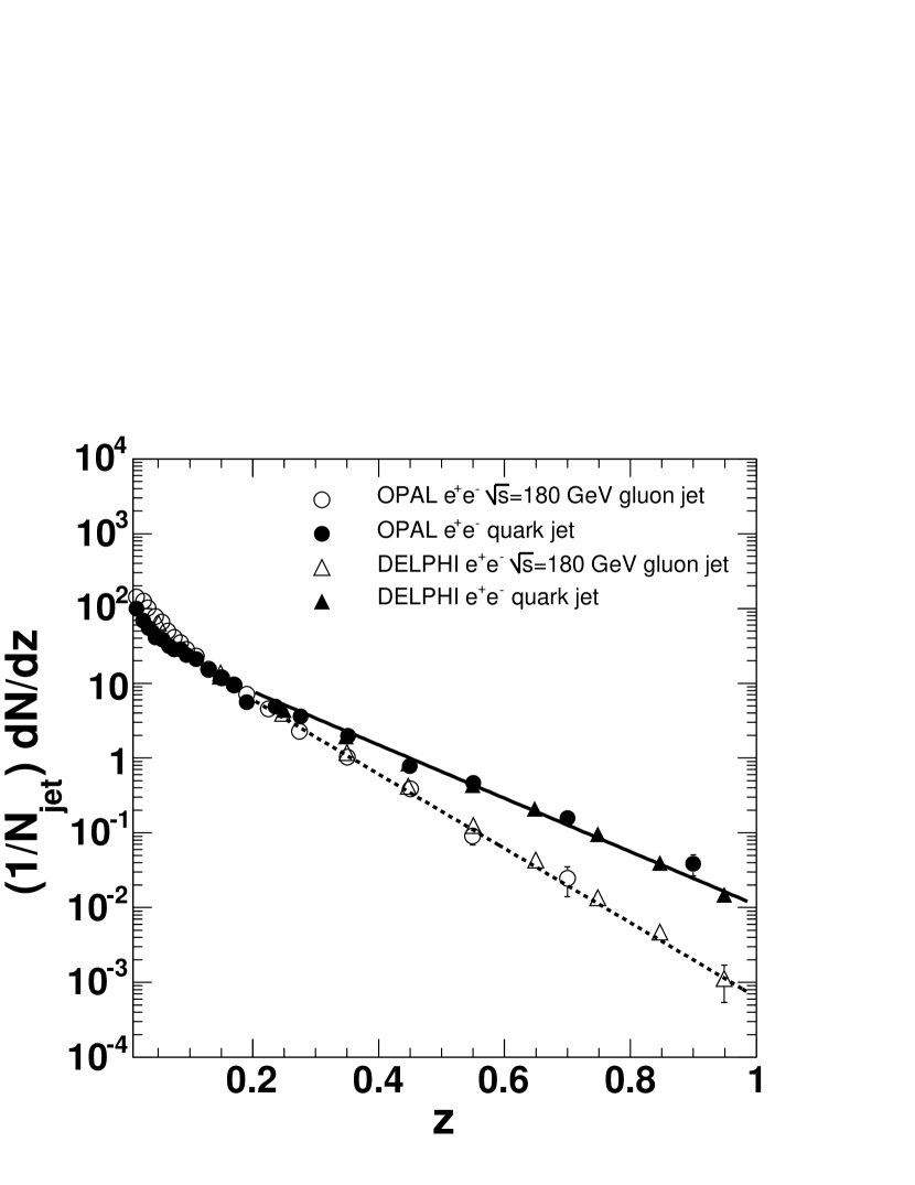
Figure 22: Fragmentation function measured in $e^{+}e^{-}$ collisions at $\sqrt{s}$=180  GeV for gluon and quark jets. The solid and dashed lines represent the exponential fit in the $0.2<z<1$ region.

The reason for the lack of convergence became apparent when we calculated $x_{E}$ distributions according to Eq. (37) (Fig. 21) for two different fragmentation functions corresponding to quark and gluon jet fragmentation. A simple exponential parameterization was used and the slopes were obtained from the fit to the LEP data Abreu et al. (2000), Alexander et al. (1996) (Fig. 22). For quark and gluon jets, we found $D_{q}(z)\approx\exp(-8.2\cdot z)$ and $D_{g}(z)\approx\exp(-11.4\cdot z)$ respectively. For the parton final state spectrum, we used $\Sigma^{\prime}_{q}\propto\hat{p}_{T\rm}^{-8}$. It is evident that the $x_{\rm E}$ distributions calculated for the quite different quark and gluon fragmentation functions do not differ significantly (the difference between solid and dashed lines on Fig. 21). Clearly, the $x_{E}$ distributions are rather insensitive to the fragmentation functions of the away jet in contradiction to the previous conventional wisdom. The evidence of this explicit counter example led to attempts to perform the integrals of Eq. (36) and Eq. (33) analytically which straightforwardly confirmed the observation that the $x_{E}$ distribution is not sensitive to the fragmentation function.

If the smeared trigger parton spectrum is taken as a power law,

$$\Sigma^{\prime}_{q}({p_{T\rm t}\over z_{\rm t}})=A({p_{T\rm t}\over z_{\rm t}})^{-(n-1)}$$

and the fragmentation function as an exponential, $D(z)=B\,\exp(-bz)$, then the integral of Eq. (36) over $z_{\rm t}$  becomes:

$${d\sigma_{\pi}\over dp_{T\rm t}dp_{T\rm a}}=$$ (38)

$${B^{2}\over\hat{x}_{\rm h}}{A\over p_{T_{t}}^{n}}\int_{x_{T_{t}}}^{\hat{x}_{\rm h}{p_{T\rm t}\over p_{T\rm a}}}dz_{\rm t}z_{\rm t}^{n-1}\exp[-bz_{\rm t}(1+{p_{T\rm a}\over{\hat{x}_{\rm h}p_{T\rm t}}})]$$

which is an incomplete gamma function. Since $\hat{x}_{h}\sim 1$, we make the assumption that it is constant. Similarly, the integrals of Eqs. 29, 33 are also incomplete gamma functions:

$${d\sigma_{\pi}\over dp_{T\rm t}}={AB\over p_{T_{t}}^{n-1}}\int_{x_{T_{t}}}^{1}dz_{\rm t}z_{\rm t}^{n-2}\exp[-bz_{\rm t}]\qquad.$$ (39)

A reasonable approximation for the inclusive single, and two particle cross sections is obtained by taking the lower limit to zero and the upper limit to infinity, leading to the replacement of the incomplete gamma functions by gamma functions, with the result that:

$${d^{2}\sigma_{\pi}\over dp_{T\rm t}dp_{T\rm a}}\approx{\Gamma(n)\over b^{n}}{B^{2}\over\hat{x}_{\rm h}}{A\over p_{T_{t}}^{n}}{1\over{(1+{p_{T\rm a}\over{\hat{x}_{\rm h}p_{T\rm t}}})^{n}}}$$ (40)

$${d\sigma_{\pi}\over dp_{T\rm t}}\approx{\Gamma(n-1)\over b^{n-1}}{AB\over p_{T_{t}}^{n-1}}\qquad,$$ (41)

where $\Gamma(n)=(n-1)\Gamma(n-1)$.

The conditional probability is just the ratio of the joint probability Eq. (40) to the inclusive probability Eq. (41), or

$$\left.{dP_{\pi}\over dp_{T\rm a}}\right|_{p_{T\rm t}}\approx{{B(n-1)}\over{bp_{T\rm t}}}{1\over\hat{x}_{\rm h}}{1\over{(1+{p_{T\rm a}\over{\hat{x}_{\rm h}p_{T\rm t}}})^{n}}}\qquad.$$ (42)

In the collinear limit, where $p_{T\rm a}$=$x_{\rm E}$$p_{T\rm t}$ :

$$\left.{dP_{\pi}\over dx_{\rm E}}\right|_{p_{T\rm t}}\approx{{B(n-1)}\over{b}}{1\over\hat{x}_{\rm h}}{1\over{(1+{x_{E}\over{\hat{x}_{\rm h}}})^{n}}}\,\qquad.$$ (43)

The only dependence on the fragmentation function, in this approximation, is in the normalization constant $B/b$ which equals $\left<m\right>$, the multiplicity in the away-jet from the integral of the fragmentation function. The dominant term in Eq. (43) is the Hagedorn function $1/(1+x_{\rm E}/\hat{x}_{\rm h})^{n}$, so that at fixed $p_{T\rm t}$ the $x_{\rm E}$ distribution is predominantly a function only of $x_{\rm E}$  and thus does exhibit ‘$x_{\rm E}$’ scaling. Also, the Hagedorn function explains the “power law” tail at large $x_{\rm E}$ noted in section V.1. The reason that the $x_{\rm E}$ distribution is not very sensitive to the fragmentation function is that the integral over $z_{\rm t}$ for fixed $p_{T\rm t}$ and $p_{T\rm a}$ (Eq. (38)) is actually an integral over the jet transverse momentum $\hat{p}_{T_{t}}$. However since both the trigger and away jets are always roughly equal and opposite in transverse momentum, integrating over $\hat{p}_{T_{t}}$ simultaneously integrates over $\hat{p}_{T_{a}}$, and thus also integrates over the away jet fragmentation function. This can be seen directly by the presence of $z_{\rm t}$ in both the same and away fragmentation functions in Eqs. 36 and 37, so that the integral over $z_{\rm t}$ integrates over both fragmentation functions simultaneously.

VI.2 $k_{T\rm}$ smearing

In order to evaluate $\hat{x}_{\rm h}$($p_{T\rm t}$,$p_{T\rm a}$) and $k_{T\rm}$ must be known. We attack this problem by successive approximations: first we solve for $k_{T}$ assuming $\hat{x}_{h}=1$ as done at the ISR, where the smearing correction was small. Then we iterate for finite $k_{T}$. The Gaussian approximation for the smearing function Eq. (35) does not work so well in the low $\hat{p}_{T\rm}$ region. The product of the steeply falling parton distribution function and the fragmentation function is peaked at $z\approx$ 1 preferring “small” parton momenta. We have developed more accurate description of the conditional yields taking into account the $k_{T\rm}$ smearing.

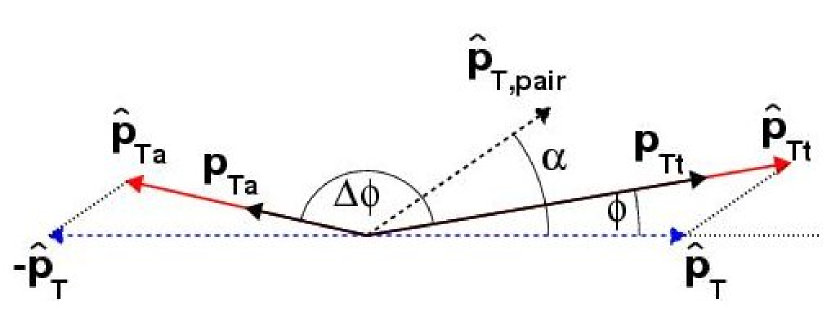
Figure 23: (color online) Back-to-back partons in hard scattering rest frame (blue dashed arrows) with four-momenta ($\hat{p}_{T\rm}$,0,0,$\hat{p}_{T\rm}$) and (-$\hat{p}_{T\rm}$,0,0,$\hat{p}_{T\rm}$) in (-,-,-,+) metrics moving along $\hat{p}_{\rm n}$ ($\hat{p}_{\rm n}=\hat{p}_{T\rm pair}$) for an event where detection of $p_{T\rm t}$ and $p_{T\rm a}$ is required (the $j_{T\rm}$ contribution is neglected). The $p_{T\rm t}$$>$ $p_{T\rm a}$ condition implies that the events with $\hat{p}_{\rm n}$ pointing more in the direction of $p_{T\rm t}$ are selected.

Let us consider the configuration depicted on Fig. 23. The two back-to-back partons in $\hat{s}$ frame undergo the Lorentz boost determined by net pair momentum

$$\vec{p}_{n}\equiv\vec{p}_{T\rm pair}\equiv\vec{\hat{p}}_{T\rm t}+\vec{\hat{p}}_{T\rm a}=\vec{k}_{T\rm t}+\vec{k}_{T\rm a}$$ (44)

If we denote an angle between the unsmeared parton momentum and $k_{T\rm}$-vector (or $\vec{p}_{n}$) as $\alpha$ (see Fig. 23) then we can write the conditional probability distribution of trigger parton momenta, $\hat{p}_{T\rm t}$, as

$${d^{3}\sigma\over d\hat{p}_{T\rm t}d\alpha d\hat{p}_{T\rm}}\Big{|}_{p_{T\rm t},p_{T\rm a}}=\hat{p}_{T\rm t}\cdot\Sigma_{q}(\hat{p}_{T})\cdot\hat{p}_{\rm n}\cdot G(\hat{p}_{\rm n}(\vec{r}_{t}))\cdot D^{q}_{\pi}({p_{T\rm t}\over\hat{p}_{T\rm t}}){p_{T\rm t}\over\hat{p}^{2}_{T\rm t}}\cdot D^{q}_{\pi}({p_{T\rm a}\over\hat{p}_{T\rm a}(\vec{r}_{t})}){p_{T\rm a}\over\hat{p}^{2}_{T\rm a}(\vec{r}_{t})}$$ (45)

where $G(\hat{p}_{\rm n})=\exp(-\hat{p}^{2}_{\rm n}/2\left<k_{T\rm}^{2}\right>)$ describes the Gaussian probability distribution of the net pair momentum magnitude distribution, $\Sigma_{q}(\hat{p}_{T})$ is the unsmeared parton momentum distribution, $D^{q}_{\pi}$ is the fragmentation function and $\vec{r}_{t}=(\hat{p}_{T\rm t},\phi,\hat{p}_{T\rm},k_{T\rm})$ is the phase space vector. The $\hat{p}_{T\rm t}$ is chosen to be an integration variable and $\hat{p}_{T\rm a}$ is fully determined by given values of $\hat{p}_{T\rm t}$, $\hat{p}_{T\rm}$, angle $\phi$ and by the requirement of Lorentz invariance.

In order to evaluate $\left<z_{\rm t}(k_{T\rm})\right>\big{|}_{p_{T\rm t},p_{T\rm a}}$ and $\hat{x}_{\rm h}(k_{T\rm})\big{|}_{p_{T\rm t},p_{T\rm a}}$ we have to evaluate first the parton distribution for events where given $p_{T\rm t}$ and $p_{T\rm a}$ are detected. This conditional cross section can be expressed as a definite integral over the unobserved variables $\phi$ and $\hat{p}_{T\rm}$ (see Fig. 23)

$${d\sigma\over d\hat{p}_{T\rm t}}\Big{|}_{p_{T\rm t},p_{T\rm a}} = 2\int_{0}^{\sqrt{s}/2}\int_{0}^{\pi}{d^{3}\sigma\over d\hat{p}_{T\rm t}d\hat{p}_{T\rm}d\phi}\Big{|}_{p_{T\rm t},p_{T\rm a}}\;d\phi d\hat{p}_{T\rm}$$

$$= D^{q}_{\pi}({p_{T\rm t}\over\hat{p}_{T\rm t}}){2\over\hat{p}_{T\rm t}}\int_{0}^{\sqrt{s}/2}\Sigma_{q}(\hat{p}_{T})\times$$

$$\times\int_{0}^{\pi}\hat{p}_{\rm n}(\vec{r}_{t})\,G(\hat{p}_{\rm n}(\vec{r}_{t}))\cdot D^{q}_{\pi}({p_{T\rm a}\over\hat{p}_{T\rm a}(\vec{r}_{t})}){1\over\hat{p}^{2}_{T\rm a}(\vec{r}_{t})}\;d\phi\;d\hat{p}_{T\rm}\quad.$$ (46)

The $d\sigma/d\hat{p}_{T\rm a}\big{|}_{p_{T\rm t},p_{T\rm a}}$ distribution can be derived from Eq. (VI.2) just by rotation $\hat{p}_{T\rm t}\rightarrow\hat{p}_{T\rm a}$ and $\hat{p}_{T\rm a}\rightarrow\hat{p}_{T\rm t}$. The $\left<z_{\rm t}(k_{T\rm})\right>\big{|}_{p_{T\rm t},p_{T\rm a}}$ and $\hat{x}_{\rm h}(k_{T\rm})\big{|}_{p_{T\rm t},p_{T\rm a}}$ quantities can then be evaluated as

$$\left<z_{\rm t}(k_{T\rm})\right>\big{|}_{p_{T\rm t},p_{T\rm a}}={\mathcal{Z}(1)\over\mathcal{Z}(0)}$$ (47)

where

$$\begin{array}[]{l}\mathcal{Z}(n)=\int_{x_{T\rm t}}^{1}z_{\rm t}^{n-1}\;D^{q}_{\pi}(z_{\rm t})\int_{0}^{\sqrt{s}/2}\Sigma_{q}(\hat{p}_{T})\times\\ \\ \times\int_{0}^{\pi}\hat{p}_{\rm n}\,G(\hat{p}_{\rm n}(\vec{r}_{zt}))\cdot D^{q}_{\pi}({p_{T\rm a}\over\hat{p}_{T\rm a}(\vec{r}_{zt})}){1\over\hat{p}^{2}_{T\rm a}(\vec{r}_{zt})}\;d\phi\;d\hat{p}_{T\rm}\;dz_{\rm t}\end{array}$$

and $\vec{r}_{zt}=(p_{T\rm t}/z_{\rm t},\phi,\hat{p}_{T\rm},k_{T\rm})$. The $\hat{x}_{\rm h}(k_{T\rm})\big{|}_{p_{T\rm t},p_{T\rm a}}$ is evaluated as

$$\hat{x}_{\rm h}(k_{T\rm})\big{|}_{p_{T\rm t},p_{T\rm a}}={\left<\hat{p}_{T\rm a}\right>\over\left<\hat{p}_{T\rm t}\right>}\Big{|}_{p_{T\rm t},p_{T\rm a}}={\mathcal{X}_{a}(1)\over\mathcal{X}_{a}(0)}{\mathcal{X}_{t}(0)\over\mathcal{X}_{t}(1)}$$ (48)

where

$$\begin{array}[]{l}\mathcal{X}_{t}(n)=\int_{p_{T\rm t}}^{\sqrt{s}/2}\hat{p}_{T\rm t}^{n-1}D^{q}_{\pi}({p_{T\rm t}\over\hat{p}_{T\rm t}})\int_{0}^{\sqrt{s}/2}\Sigma_{q}(\hat{p}_{T})\times\\ \\ \times\int_{0}^{\pi}\hat{p}_{\rm n}(\vec{r}_{t})\,G(\hat{p}_{\rm n}(\vec{r}_{t}))\cdot D^{q}_{\pi}({p_{T\rm a}\over\hat{p}_{T\rm a}(\vec{r}_{t})}){1\over\hat{p}^{2}_{T\rm a}(\vec{r}_{t})}\;d\phi\;d\hat{p}_{T\rm}\hat{p}_{T\rm t}\\ \\ \mathcal{X}_{a}(n)=\int_{p_{T\rm a}}^{\sqrt{s}/2}\hat{p}_{T\rm a}^{n-1}D^{q}_{\pi}({p_{T\rm a}\over\hat{p}_{T\rm a}})\int_{0}^{\sqrt{s}/2}\Sigma_{q}(\hat{p}_{T})\times\\ \\ \times\int_{0}^{\pi}\hat{p}_{\rm n}(\vec{r}_{a})\,G(\hat{p}_{\rm n}(\vec{r}_{a}))\cdot D^{q}_{\pi}({p_{T\rm t}\over\hat{p}_{T\rm t}(\vec{r}_{a})}){1\over\hat{p}^{2}_{T\rm t}(\vec{r}_{a})}\;d\phi\;d\hat{p}_{T\rm}\hat{p}_{T\rm a}\end{array}$$

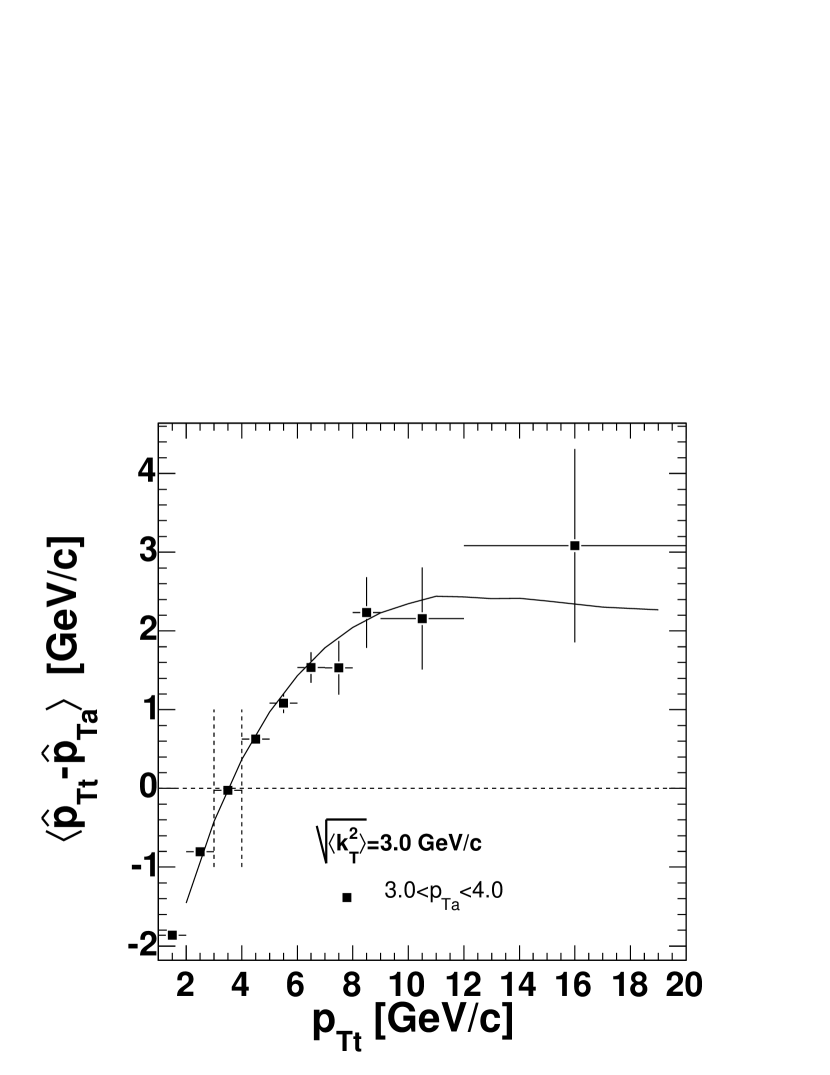
Figure 24: PYTHIA simulated average momentum unbalance for the associated particles in $3.0<p_{T\rm a}<4.0$  GeV/$c$ bin and calculated according Eq. (48). The two vertical dashed line indicates the range where $p_{T\rm t}$ and $p_{T\rm a}$ bins are equal and the parton momenta unbalance vanishes (fixed correlations).

We have tested the above formulae on PYTHIA simulation. We have generated events with $\sqrt{\left<k_{T\rm}^{2}\right>}$=3  GeV/$c$ and evaluated the partons’ momenta unbalance variation with $p_{T\rm t}$ for fixed $3<p_{T\rm a}<4$  GeV/$c$ bin. The results from the PYTHIA simulation (solid point on Fig. 24) are compared to calculation based on Eq. (48) (solid line on Fig. 24). The magnitude of momentum unbalance saturates at $p_{T\rm t}$$\approx$10 GeV/$c$ around $\sqrt{\left<k_{T\rm x}^{2}\right>}$ and then starts to decrease. The maximum value depends on the the $k_{T\rm}$ magnitude and on the asymmetry between $p_{T\rm t}$ and $p_{T\rm a}$. Eventually, the unbalance should vanish at high $p_{T\rm t}$ as a consequence of $\Sigma_{q}(\hat{p}_{T})$ flattening.

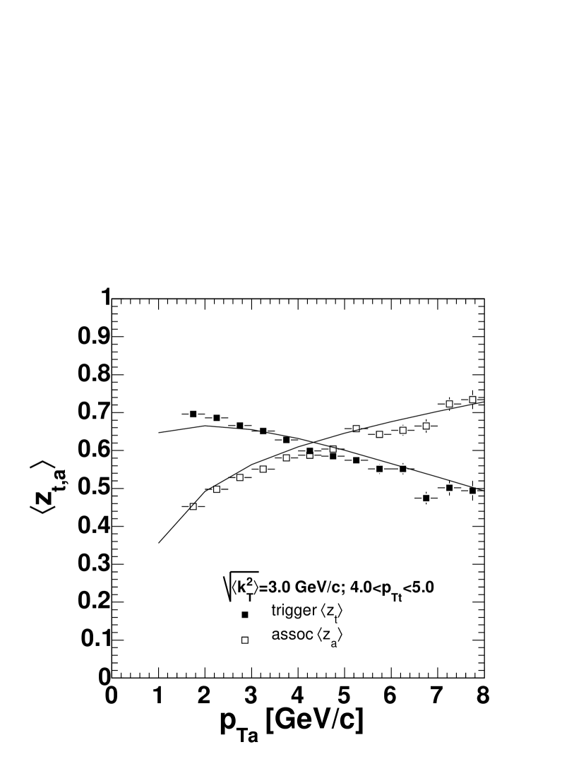
Figure 25: Average $z$ of a trigger and associated particle as a function of $p_{T\rm a}$ from PYTHIA and according Eq. (47).

The comparison of $\left<z_{\rm t}\right>$ and $\left<z_{\rm a}\right>$ found in PYTHIA and derived according to Eq. (47) is shown in Fig. 25. The overall agreement between the PYTHIA simulations and the calculation is excellent. The small deviations may be attributed to the fact that in the PYTHIA simulation, 1 GeV/$c$-wide bins were used for trigger and associated particle identification, whereas the calculation was performed for fixed values of $p_{T\rm t}$ and $p_{T\rm a}$.

The last missing piece of information needed before solving Eq. (22) is the fragmentation function $D^{q}_{\pi}$ and unsmeared $\Sigma_{q}(\hat{p}_{T})$. The description of how this knowledge was extracted from the data is a subject of next section.

VII Corrected $\left<k_{T\rm}\right>$ results

The $\hat{x}_{\rm h}^{-1}\left<z_{\rm t}\right>\sqrt{\left<k_{T\rm}^{2}\right>}$ extracted according to Eq. (22) for various $p_{T\rm t}$ and $p_{T\rm a}$ are shown in Fig. 16 and Fig. 17. In order to extract a $\sqrt{\left<k_{T\rm}^{2}\right>}$ values we have solved

$$x_{\rm h}^{-1}\sqrt{\left<p_{\rm out}^{2}\right>-\left<j_{T\rm y}^{2}\right>(x_{\rm h}^{2}+1)}-\hat{x}_{\rm h}^{-1}\left<z_{\rm t}\right>\sqrt{\left<k_{T\rm}^{2}\right>}=0$$ (49)

for $\sqrt{\left<k_{T\rm}^{2}\right>}$ where the $\left<z_{\rm t}\right>$ and $\hat{x}_{\rm h}$=$\left<\hat{p}_{T\rm a}\right>$/$\left<\hat{p}_{T\rm t}\right>$ are evaluated according Eq. (47) and Eq. (48) respectively. These two quantities depend on $\sqrt{\left<k_{T\rm}^{2}\right>}$ so we solved Eq. (49) iteratively by varying a $\sqrt{\left<k_{T\rm}^{2}\right>}$ value and in every step the $\left<z_{\rm t}\right>$ and $\hat{x}_{\rm h}$ were recalculated. To do so the we need to know unsmeared final state parton spectrum $\Sigma_{q}(\hat{p}_{T})$ and the fragmentation function. For the latter one we used the LEP data (see Fig. 22) where the fragmentation functions of gluon and quark jets were measured in $e^{+}e^{-}$ collision at $\sqrt{s}$=180  GeV. We have chosen

$$D^{q}_{\pi}\propto z^{-\alpha}(1-z)^{\beta}(1+z)^{-\gamma}$$ (50)

form used e.g. in Abreu et al. (2000) and extracted $\alpha$, $\beta$ and $\gamma$ parameters from the fit to distributions shown in Fig. 22 (see Tab. 8).

Table 8: Extracted values of $D(z)$ parameters according Eq. (50) from the fit to the LEP data and power $n$ of the unsmeared final state parton spectra $\Sigma_{q}(\hat{p}_{T})$ extracted from the fit to the single inclusive $\pi^{0}$ invariant cross section Adler et al. (2003e) for corresponding fragmentation function and fixed value of $\sqrt{\left<k_{T\rm}^{2}\right>}$=2.5  GeV/$c$.

	gluon	quark	(gluon+quark)/2
$\alpha$	0.16	0.49	0.32
$\beta$	0.88	0.57	0.72
$\gamma$	13.29	8.00	10.65
$n$	7.53	7.28	7.40

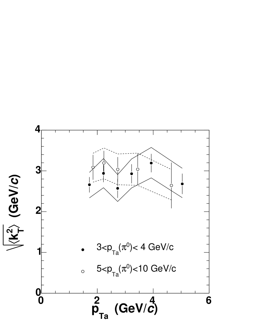
Figure 26: $\sqrt{\left<k_{T\rm}^{2}\right>}$ values corresponding to Fig. 16 as a solution to Eq. (49) for trigger $\pi^{0}$ in $3<p_{T\rm t}<4$ GeV/$c$ (solid symbols) and $5<p_{T\rm t}<10$ GeV/$c$ (open symbols) range. The solid and dashed lines bracket the systematic uncertainty due to the unknown ratio of quark and gluon jets, for the solid and open symbols, respectively.

For a given set of parameters $\alpha$, $\beta$ and $\gamma$ the power of the unsmeared final state parton spectra $\Sigma_{q}(\hat{p}_{T})$ was evaluated from the fit formula Eq. (27) to the single inclusive $\pi^{0}$ invariant cross section Adler et al. (2003e). Here we used the simplified $k_{T\rm}$ smearing

$$f^{\prime}_{q}(\hat{p}_{T\rm t})={1\over\hat{p}_{T\rm t}}\Sigma^{\prime}_{q}(\hat{p}_{T\rm t})={1\over\hat{p}_{T\rm}}\Sigma_{q}(\hat{p}_{T})\otimes\exp{-(\hat{p}_{T\rm}-\hat{p}_{T\rm t})^{2}\over\left<k_{T\rm x}^{2}\right>}$$

and for the fixed value of $\sqrt{\left<k_{T\rm}^{2}\right>}$ = $\sqrt{2}$$\sqrt{\left<k_{T\rm x}^{2}\right>}$ = 2.5  GeV/$c$ the power $n$ of $\Sigma_{q}(\hat{p}_{T})$ distribution was determined.

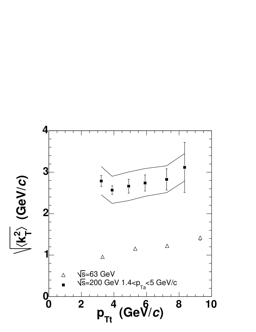
Figure 27: $\sqrt{\left<k_{T\rm}^{2}\right>}$ values corresponding to Fig. 17 as a solution to Eq. (49) for associated particles in $1.4<p_{T\rm a}<5$ GeV/$c$ region (solid symbols). The solid lines bracket the systematic error due to the unknown ratio of quark and gluon jets. The CCOR measurement at $\sqrt{s}$=62.4  GeV Angelis et al. (1980) (empty triangles).

The measurement of the fragmentation functions at LEP was done separately for quark and gluon jets and the slopes of these two $D(z)$ distributions are different. Quark jets produce a significantly harder spectrum than gluon jets (see Fig. 22). Since the relative abundance of quark and gluon jets at $\sqrt{s}$=200  GeV is not known, for the final results we assumed that the numbers of quark and gluon jets are equal; the final $D(z)$ uses the averaged parameter values between quark and gluon and the difference was used as a measure of the systematic uncertainty.

Figure 28: $\left<z_{\rm t}\right>$ and $\hat{x}_{\rm h}$ as a function of $p_{T\rm t}$ for the $1.4<p_{T\rm a}<5.0$  GeV/$c$ associated region.

Resulting $\sqrt{\left<k_{T\rm}^{2}\right>}$ values for $3<p_{T\rm t}<4$ GeV/$c$ and $5<p_{T\rm t}<10$ GeV/$c$ as a function of $p_{T\rm a}$ are shown in Fig. 26 (compare to uncorrected values Fig. 17). The solid and dashed lines bracket the systematic error due to the unknown ratio of quark and gluon jets. These data points correspond to the uncorrected $\hat{x}_{\rm h}^{-1}\left<z_{\rm t}\right>\sqrt{\left<k_{T\rm}^{2}\right>}$ values shown in Fig. 16. The $\sqrt{\left<k_{T\rm}^{2}\right>}$ values for varying $p_{T\rm t}$ corresponding to the data shown of Fig. 17 are shown in Fig. 27. Also here the solid lines bracket the systematic error due to the unknown ratio of quark and gluon jets. It is evident that unfolded $\sqrt{\left<k_{T\rm}^{2}\right>}$ values reveal, within the error bars, no dependence neither on $p_{T\rm a}$ nor on $p_{T\rm t}$. The tabulated data are given in Table 9.

Table 9: Values of $\hat{x}_{\rm h}^{-1}\left<z_{\rm t}\right>\sqrt{\left<k_{T\rm}^{2}\right>}$ and $\sqrt{\left<k_{T\rm}^{2}\right>}$ for various trigger particle $p_{T\rm t}$ and associated momenta in the $1.4<p_{T\rm a}<5.0$  GeV/$c$ region shown in Fig. 17 and Fig. 27

$p_{T\rm t}$	$\hat{x}_{\rm h}^{-1}\left<z_{\rm t}\right>\sqrt{\left<k_{T\rm}^{2}\right>}$	$\sqrt{\left<k_{T\rm}^{2}\right>}$
GeV/$c$	GeV/$c$	GeV/$c$
3.22	1.63 $\pm$ 0.08	2.79 $\pm$ 0.13 $\pm$ 0.35
3.89	1.66 $\pm$ 0.08	2.57 $\pm$ 0.11 $\pm$ 0.33
4.90	1.89 $\pm$ 0.13	2.66 $\pm$ 0.17 $\pm$ 0.35
5.91	2.06 $\pm$ 0.19	2.74 $\pm$ 0.20 $\pm$ 0.34
7.24	2.17 $\pm$ 0.25	2.83 $\pm$ 0.25 $\pm$ 0.32
8.34	2.53 $\pm$ 0.62	3.11 $\pm$ 0.60 $\pm$ 0.33

We compared the $\sqrt{\left<k_{T\rm}^{2}\right>}$ data obtained in this analysis to $\sqrt{\left<k_{T\rm}^{2}\right>}$ values found by the CCOR collaboration at $\sqrt{s}$=62.4  GeV Angelis et al. (1980) (empty triangles on Fig. 27). Although the trend with $p_{T\rm t}$ seems to be similar the overall magnitude at $\sqrt{s}$=200  GeV is significantly higher.

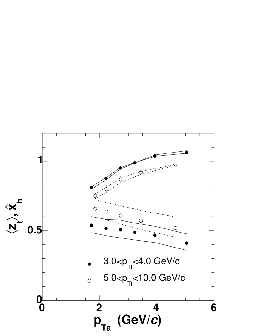
Figure 29: The $\left<z_{\rm t}\right>$ and $\hat{x}_{\rm h}$ values (see Eq. 20) as solution of Eq. (48) for $3<p_{T\rm t}<4$ GeV/$c$ and $5<p_{T\rm t}<10$ GeV/$c$ as a function of $p_{T\rm a}$ .

Table 10: The $\hat{x}_{\rm h}^{-1}\left<z_{\rm t}\right>\sqrt{\left<k_{T\rm}^{2}\right>}$ $\sqrt{\left<k_{T\rm}^{2}\right>}$ values as a function of $p_{T\rm a}$ for two different trigger $\pi^{0}$ transverse momentum bins shown in Fig. 16 and Fig. 26. All units in rad and  GeV/$c$.

$3<p_{T\rm t}<4$			$5<p_{T\rm t}<10$
$p_{T\rm a}$	$\left<z_{\rm t}\right>\sqrt{\left<k_{T\rm}^{2}\right>}\over\hat{x}_{\rm h}$	$\sqrt{\left<k_{T\rm}^{2}\right>}$	$p_{T\rm a}$	$\left<z_{\rm t}\right>\sqrt{\left<k_{T\rm}^{2}\right>}\over\hat{x}_{\rm h}$	$\sqrt{\left<k_{T\rm}^{2}\right>}$
1.7	1.76 $\pm$ 0.12	2.66 $\pm$ 0.19	1.9	2.69 $\pm$ 0.37	3.09 $\pm$ 0.30
2.2	1.74 $\pm$ 0.13	2.94 $\pm$ 0.22	2.2	2.54 $\pm$ 0.31	3.19 $\pm$ 0.30
2.7	1.37 $\pm$ 0.13	2.57 $\pm$ 0.23	2.7	2.13 $\pm$ 0.26	3.04 $\pm$ 0.30
3.2	1.45 $\pm$ 0.12	2.93 $\pm$ 0.23	3.4	1.89 $\pm$ 0.27	3.04 $\pm$ 0.38
3.9	1.44 $\pm$ 0.11	3.19 $\pm$ 0.23	4.7	1.41 $\pm$ 0.30	2.64 $\pm$ 0.56
5.0	1.04 $\pm$ 0.10	2.68 $\pm$ 0.25

The $\left<z_{\rm t}\right>$ and $\hat{x}_{\rm h}$ values from the iterative solution of Eq. (49) as a function of the $\pi^{0}$trigger momenta $p_{T\rm t}$ and associated momenta $p_{T\rm a}$ are shown in Fig. 28 and Fig. 29. There is an opposite trend; whereas the $\left<z_{\rm t}\right>$ rises with $p_{T\rm t}$ it is falling with $p_{T\rm a}$. It is an interesting consequence of two effects: competition between steeply falling final state parton spectra and rising fragmentation function with parton momentum. Secondly, the detection of trigger particle biases the $\vec{k}_{T\rm}$ vector in the direction of the trigger jet as discussed in section VI.2.

Table 11: The $\left<z_{\rm t}\right>$ and $\hat{x}_{\rm h}$ values with $p_{T\rm t}$ shown in Fig. 28.

$p_{T\rm t}$ ( GeV/$c$)	$\left<z_{\rm t}\right>$	$\hat{x}_{\rm h}$
3.22	0.51 $\pm$ 4.10-3 $\pm$ 0.06	0.88 $\pm$ 0.01
3.89	0.56 $\pm$ 2.10-3 $\pm$ 0.07	0.87 $\pm$ 0.01
4.90	0.61 $\pm$ 1.10-3 $\pm$ 0.07	0.85 $\pm$ 0.01
5.91	0.64 $\pm$ 1.10-4 $\pm$ 0.07	0.85 $\pm$ 0.02
7.24	0.66 $\pm$ 1.10-3 $\pm$ 0.07	0.86 $\pm$ 0.02
8.34	0.68 $\pm$ 5.10-3 $\pm$ 0.06	0.84 $\pm$ 0.05

Table 12: The $\left<z_{\rm t}\right>$ and $\hat{x}_{\rm h}$ values with $p_{T\rm a}$ for two trigger $\pi^{0}$ momenta bins as shown on Fig. 29.

$3<p_{T\rm t}<4$  GeV/$c$
$p_{T\rm a}$	$\left<z_{\rm t}\right>$	$\hat{x}_{\rm h}$
1.72	0.54 $\pm$ 8.10-3 $\pm$ 0.06	0.81 $\pm$ 0.01
2.22	0.52 $\pm$ 6.10-3 $\pm$ 0.06	0.88 $\pm$ 0.01
2.73	0.51 $\pm$ 1.10-3 $\pm$ 0.07	0.95 $\pm$ 0.01
3.23	0.49 $\pm$ 1.10-3 $\pm$ 0.06	0.99 $\pm$ 0.01
3.93	0.47 $\pm$ 5.10-3 $\pm$ 0.06	1.04 $\pm$ 0.01
5.04	0.41 $\pm$ 6.10-3 $\pm$ 0.06	1.06 $\pm$ 0.01
$5<p_{T\rm t}<10$  GeV/$c$
$p_{T\rm a}$	$\left<z_{\rm t}\right>$	$\hat{x}_{\rm h}$
1.85	0.66 $\pm$ 4.10-3 $\pm$ 0.06	0.75 $\pm$ 0.04
2.24	0.64 $\pm$ 1.10-3 $\pm$ 0.06	0.80 $\pm$ 0.03
2.73	0.61 $\pm$ 2.10-3 $\pm$ 0.07	0.87 $\pm$ 0.02
3.44	0.57 $\pm$ 2.10-3 $\pm$ 0.07	0.92 $\pm$ 0.02
4.65	0.52 $\pm$ 5.10-3 $\pm$ 0.08	0.98 $\pm$ 0.01

The $p_{T\rm t}$ averaged value of $\sqrt{\left<k_{T\rm}^{2}\right>}$ (Fig. 27) is compared to the average parton pair momentum, $\left<\hat{p}_{\rm n}\right>$ =$\left<p_{T\rm}\right>$_pair, presented in Apanasevich et al. (1999) (see Fig. 30). The value of $\left<p_{T\rm}\right>$_pair is determined as a sum of the two partons’ $\left<k_{T\rm}\right>$. In the present analysis the $\sqrt{\left<k_{T\rm}^{2}\right>}$ is determined and thus the value of $\left<p_{T\rm}\right>$_pair is evaluated as $\left<p_{T\rm}\right>_{pair}=\sqrt{2}\times\left<k_{T\rm}\right>=\sqrt{\pi/2}\times\sqrt{\left<k_{T\rm}^{2}\right>}.$

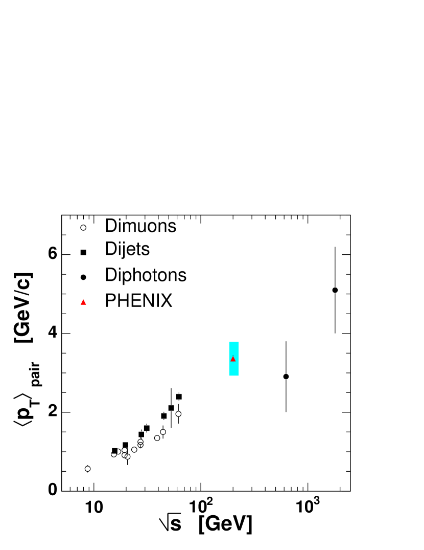
Figure 30: (color online) Compilation of mean pair $p_{T\rm}$ measurements Apanasevich et al. (1999) and comparisons to the $\left<p_{T\rm}\right>$_pair measured in this analysis.

The present value of $\left<p_{T\rm}\right>$_pair

$$\left<p_{T\rm}\right>_{pair}=3.36\pm 0.09(\rm stat)\pm 0.43(\rm sys)\mbox{~{}GeV/$c$}$$

appears to be in a good agreement with the lower energy dijet and dilepton measurements or the higher energy measurement in diphoton production Abe et al. (1993). A UA2 measurement of $\left<p_{T\rm}\right>$ of $Z^{0}$ production at $\sqrt{s}\sim 600$  GeV gives $8.6\pm 1.5$ GeV/c Ansari et al. (1987, 1988).

VIII Summary

We have made the first measurement of jet $j_{T\rm}$ and $k_{T\rm}$ for $p+p$ collisions at $\sqrt{s}$ = 200  GeV using the method of two-particle correlations. Analysis of the angular widths of the near-side peak in the correlation function has determined that the jet fragmentation transverse momentum $j_{T\rm}$ is constant with trigger particle $p_{T\rm t}$ and the extracted value $\sqrt{\left<j_{T\rm}^{2}\right>}=585\pm 6(\rm stat)\pm 15(\rm sys)\mbox{~{}MeV/$c$}$ is comparable with previous lower $\sqrt{s}$ measurements. The width of the away-side peak is shown to be a measure of the convolution of $j_{T\rm}$ with the jet momentum fraction $z$ and the partonic transverse momentum $k_{T\rm}$. $\left<z_{\rm t}\right>$ is determined through a combined analysis of the measured $\pi^{0}$ inclusive and associated spectra using the jet fragmentation functions from $e^{+}e^{-}$ measurements. The average of $\left<z_{\rm t}\right>$ from the gluon and quark fragmentation functions is used and the difference is taken as the measure of the systematic error. The final extracted values of $k_{T\rm}$ are then determined to be also independent of the transverse momentum of the trigger $\pi^{0}$, in the range measured, with values of $\sqrt{\left<k_{T\rm}^{2}\right>}=2.68\pm 0.07(\rm stat)\pm 0.34(\rm sys)\mbox{~{}GeV/$c$}$.

Appendix A

A.1 First and second moments of normally distributed quantities

Let $x$ be a 1D variable with normal (Gaussian) distribution and $r=\sqrt{x^{2}+y^{2}}$ is a 2D variable with $x$ and $y$ of normal distribution then the following relations can be easily derived $\left<x\right>$ = 0 $\left<r\right>$ = $\sqrt{\pi\over 2}\sigma_{1}$ $\left<|x|\right>$ = $\sqrt{2\over\pi}\sigma_{1}$ $\left<|r|\right>$ = $\left<r\right>$ $\left<x^{2}\right>$ = $\sigma^{2}_{1}$ $\left<r^{2}\right>$ = $2\sigma^{2}_{1}\equiv\sigma^{2}_{2}$

Both $\vec{j}_{T\rm\ }$and $\vec{k}_{T\rm}$ are two dimensional vectors. We assume Gaussian distributed $x$ and $y$ components and thus the mean value $\left<k_{T\rm}x\right>$ and $\left<k_{T\rm y}\right>$ is equal to zero. The non-zero moments of 2D Gaussian distribution are e.g. the root mean squares $\sqrt{\left<j_{T}^{2}\right>}$, $\sqrt{\left<k_{T}^{2}\right>}$ or the mean absolute values of the $\vec{j}_{T\rm,}$ $\vec{k}_{T\rm}$ projections into the perpendicular plane to the jet axes $\left<|j_{T\rm y}|\right>$ and $\left<|k_{T\rm y}|\right>$. Note that there are a trivial correspondences

$$\sqrt{\left<k_{T\rm}^{2}\right>}={2\over\sqrt{\pi}}\left<k_{T\rm}\right>=\sqrt{\pi}\left<|k_{T\rm y}|\right>\\$$ (51)

A.2 The correct way to analyze the azimuthal correlation function.

Construction and fitting of the two-particle azimuthal correlation function is discussed in section IV. Traditionally the correlation function is fitted by two Gaussian functions - one for intra-jet correlation (near peak) and one for the inter-jet correlations (away-side peak). From the extracted variances of the Gaussian functions the $j_{T\rm}$ and $p_{\rm out}$ magnitudes are extracted.

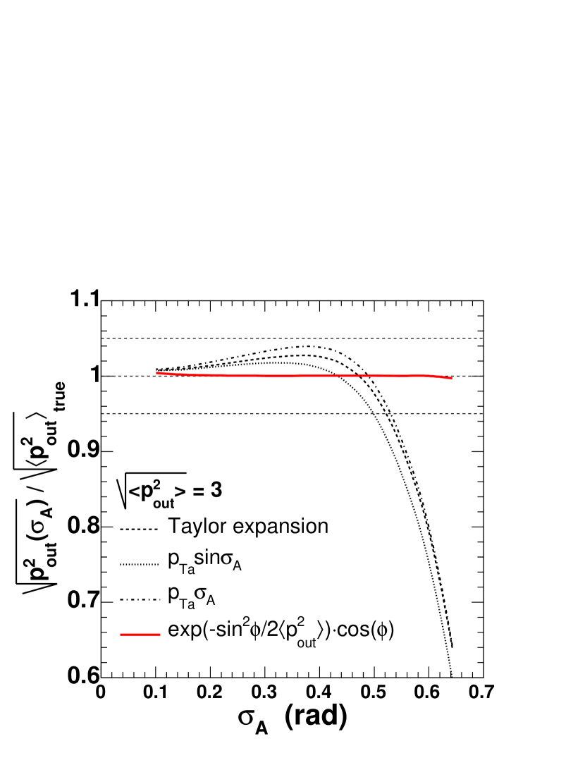
Figure 31: (color online) The relative error on $p_{\rm out}$ determination from the azimuthal correlation function based on the Taylor expansion of $\left<\sin\Delta\phi^{2}\right>$ (dashed line), with an assumption of $\sqrt{\left<p_{\rm out}^{2}\right>}$=$p_{T\rm a}$ sin$\sigma_{\rm A}$ (dotted line) and $\sqrt{\left<p_{\rm out}^{2}\right>}$=$p_{T\rm a}$$\sigma_{\rm A}$ (dotted-dashed line). The solid red line corresponds to $\sqrt{\left<p_{\rm out}^{2}\right>}$ from Eq. (23).

There is, however, a fundamental problem with this approach. The $p_{\rm out}$-vector defined in Eq. (17) is equal to $p_{T\rm a}\sin\Delta\phi$ event by event. However, we measure the width of the correlation peak and this corresponds to $\sqrt{\left<\Delta\phi^{2}\right>}=\sigma_{\rm A}$. The relation $\sqrt{\left<p_{\rm out}^{2}\right>}$$\approx p_{T\rm a}\sin\sigma_{\rm A}$ is not a good approximation for $\sigma_{\rm A}$$>$0.4 rad (see Fig. 31). The assumption that the away-side correlation has a Gaussian shape is also good only for small values of $\sigma_{\rm A}$ (see Fig. 31).

One way of relating $\sqrt{\left<p_{\rm out}^{2}\right>}$ and $\sigma_{\rm A}$ was proposed e.g. by Peter Levai Levai et al. and used in several other analyzes. Since $\sqrt{\left<p_{\rm out}^{2}\right>}$=$p_{T\rm a}\sqrt{\left<\sin^{2}\Delta\phi\right>}$ one possibility how to relate $p_{\rm out}$ and $\sigma_{\rm A}$ is to expand

$$\left<\sin^{2}\Delta\phi\right> = \left<\Delta\phi^{2}-{1\over 3}\Delta\phi^{4}+{2\over 45}\Delta\phi^{6}\dots\right>$$

$$= \sigma_{\rm A}^{2}-\sigma_{\rm A}^{4}+{2\over 3}\sigma_{\rm A}^{6}\dots$$

where we assumed a Gaussian distribution of $\Delta\phi$. The comparison of $p_{T\rm a}\cdot(\sigma_{\rm A}^{2}-\sigma_{\rm A}^{4}+{2\over 3}\sigma_{\rm A}^{6}\dots)$ with the true $p_{\rm out}$ magnitude (simple monte carlo) for various $\sigma_{\rm A}$ values is shown in Fig. 31. It is obvious that there is only a little difference between $\sqrt{\left<p_{\rm out}^{2}\right>}$=$p_{T\rm a}$ sin$\sigma_{\rm A}$, $\sqrt{\left<p_{\rm out}^{2}\right>}$=$p_{T\rm a}$$\sigma_{\rm A}$ and the Taylor series. In the region where $\sigma_{\rm A}$$>$0.4 rad, all approximations seems to be equally bad.

However, $p_{\rm out}$, the only quantity with a truly Gaussian distribution (if we neglect the radiative corrections responsible for non-Gaussian tails in the $p_{\rm out}$ distribution which are anyway not relevant for the $k_{T\rm}$ analysis) can be directly extracted from the correlation function. With the assumption of Gaussian distribution in $p_{\rm out}$, we can write the away-side $\Delta\phi$-distribution (normalized to unity) as

$${dN_{away}\over d\Delta\phi}\Big{|}_{\pi/2}^{3\pi/2}={dN\over dp_{\rm out}}{dp_{\rm out}\over d\Delta\phi}=$$

$$={-p_{T\rm a}\cos\Delta\phi\over\sqrt{2\pi\left<p_{\rm out}^{2}\right>}{\rm Erf}({\sqrt{2}p_{T\rm a}\over\sqrt{\left<p_{\rm out}^{2}\right>}})}\exp\left(-{p^{2}_{T\rm a}\sin^{2}\Delta\phi\over 2\left<p_{\rm out}^{2}\right>}\right)$$

This is the correct way of extracting a dimensional quantity from the azimuthal correlation function in the case of narrow associated bin. Similar line of arguments can be drawn also in the case of near peak. However, given the narrowness of the near angle peak, the simple Gaussian approximation is good enough.

References

- Angelis et al. (1980) A. L. S. Angelis et al. (CERN-Columbia-Oxford-Rockefeller), Phys. Lett. B97, 163 (1980).
- Darriulat et al. (1976) P. Darriulat et al., Nucl. Phys. B107, 429 (1976).
- Della Negra et al. (1977) M. Della Negra et al. (CERN-College de France-Heidelberg-Karlsruhe), Nucl. Phys. B127, 1 (1977).
- Adcox et al. (2002) K. Adcox et al. (PHENIX), Phys. Rev. Lett. 88, 022301 (2002), eprint nucl-ex/0109003.
- Adler et al. (2003a) S. S. Adler et al. (PHENIX), Phys. Rev. Lett. 91, 072303 (2003a), eprint nucl-ex/0306021.
- Adler et al. (2003b) S. S. Adler et al. (PHENIX), Phys. Rev. Lett. 91, 182301 (2003b), eprint nucl-ex/0305013.
- Adler et al. (2003c) C. Adler et al. (STAR), Phys. Rev. Lett. 90, 032301 (2003c), eprint nucl-ex/0206006.
- Adler et al. (2003d) C. Adler et al. (STAR), Phys. Rev. Lett. 90, 082302 (2003d), eprint nucl-ex/0210033.
- Migdal (1956) A. B. Migdal, Phys. Rev. 103, 1811 (1956).
- Wang and Gyulassy (1992) X.-N. Wang and M. Gyulassy, Phys. Rev. Lett. 68, 1480 (1992).
- Wang (1998) X.-N. Wang, Phys. Rev. C58, 2321 (1998), eprint hep-ph/9804357.
- Salgado and Wiedemann (2004) C. A. Salgado and U. A. Wiedemann, Phys. Rev. Lett. 93, 042301 (2004), eprint hep-ph/0310079.
- Qiu and Vitev (2003) J.-w. Qiu and I. Vitev, Phys. Lett. B570, 161 (2003), eprint nucl-th/0306039.
- Wang (2002) X.-N. Wang, Nucl. Phys. A702, 238 (2002), eprint hep-ph/0208094.
- Berman et al. (1971a) S. M. Berman, J. D. Bjorken, and J. B. Kogut, Phys. Rev. D4, 3388 (1971a).
- Owens and Kimel (1978) J. F. Owens and J. D. Kimel, Phys. Rev. D18, 3313 (1978).
- Owens et al. (1978) J. F. Owens, E. Reya, and M. Gluck, Phys. Rev. D18, 1501 (1978).
- Feynman et al. (1978) R. P. Feynman, R. D. Field, and G. C. Fox, Phys. Rev. D18, 3320 (1978).
- Owens (1987) J. F. Owens, Rev. Mod. Phys. 59, 465 (1987).
- Bunce et al. (2000) G. Bunce, N. Saito, J. Soffer, and W. Vogelsang, Ann. Rev. Nucl. Part. Sci. 50, 525 (2000), eprint hep-ph/0007218.
- Cutler and Sivers (1978) R. Cutler and D. W. Sivers, Phys. Rev. D17, 196 (1978).
- Cutler and Sivers (1977) R. Cutler and D. W. Sivers, Phys. Rev. D16, 679 (1977).
- Combridge et al. (1977) B. L. Combridge, J. Kripfganz, and J. Ranft, Phys. Lett. B70, 234 (1977).
- Feynman et al. (1977) R. P. Feynman, R. D. Field, and G. C. Fox, Nucl. Phys. B128, 1 (1977).
- (25) Y. L. Dokshitzer, V. A. Khoze, A. H. Mueller, and S. I. Troian, Basics of perturbative qcd, gif-sur-Yvette, France: Ed. Frontieres (1991) 274 p. (Basics of).
- Apanasevich et al. (1999) L. Apanasevich et al., Phys. Rev. D59, 074007 (1999), eprint hep-ph/9808467.
- Kulesza et al. (2003) A. Kulesza, G. Sterman, and W. Vogelsang, Nucl. Phys. A721, 591 (2003), eprint hep-ph/0302121.
- Busser et al. (1973) F. W. Busser et al., Phys. Lett. B46, 471 (1973).
- Berman et al. (1971b) S. M. Berman, J. D. Bjorken, and J. B. Kogut, Phys. Rev. D4, 3388 (1971b).
- Blankenbecler et al. (1972) R. Blankenbecler, S. J. Brodsky, and J. F. Gunion, Phys. Lett. B42, 461 (1972).
- Antreasyan et al. (1979) D. Antreasyan et al., Phys. Rev. D19, 764 (1979).
- Darriulat (1980) P. Darriulat, Ann. Rev. Nucl. Part. Sci. 30, 159 (1980).
- Adachi et al. (1999) K. Adachi et al. (TOPAZ), Phys. Lett. B451, 256 (1999), eprint hep-ex/9901036.
- Adcox et al. (2003a) K. Adcox et al. (PHENIX), Nucl. Instrum. Meth. A499, 469 (2003a).
- Aphecetche et al. (2003a) L. Aphecetche et al. (PHENIX), Nucl. Instrum. Meth. A499, 521 (2003a).
- Adcox et al. (2003b) K. Adcox et al. (PHENIX), Nucl. Instrum. Meth. A499, 489 (2003b).
- Adler et al. (2003e) S. S. Adler et al. (PHENIX), Phys. Rev. Lett. 91, 241803 (2003e), eprint hep-ex/0304038.
- Aphecetche et al. (2003b) L. Aphecetche et al. (PHENIX), Nucl. Instrum. Meth. A499, 521 (2003b).
- Aizawa et al. (2003) M. Aizawa et al. (PHENIX), Nucl. Instrum. Meth. A499, 508 (2003).
- Adler et al. (2004) S. S. Adler et al. (PHENIX), Phys. Rev. C69, 034910 (2004), eprint nucl-ex/0308006.
- Adler et al. (2005) S. S. Adler et al. (PHENIX), Phys. Rev. Lett. 94, 082301 (2005), eprint nucl-ex/0409028.
- (42) P. Levai, G. Fai, and G. Papp, Dijet correlations at isr and rhic energies, eprint hep-ph/0502238.
- Adams et al. (2003) J. Adams et al. (STAR), Phys. Rev. Lett. 91, 072304 (2003), eprint nucl-ex/0306024.
- van Apeldoorn et al. (1975) G. W. van Apeldoorn et al., Nucl. Phys. B91, 1 (1975).
- Wang (2004) X.-N. Wang, Phys. Lett. B595, 165 (2004), eprint nucl-th/0305010.
- Abreu et al. (2000) P. Abreu et al. (DELPHI), Eur. Phys. J. C13, 573 (2000).
- Alexander et al. (1996) G. Alexander et al. (OPAL), Z. Phys. C69, 543 (1996).
- Abe et al. (1993) F. Abe et al. (CDF), Phys. Rev. Lett. 70, 2232 (1993).
- Ansari et al. (1987) R. Ansari et al. (UA2), Phys. Lett. B194, 158 (1987).
- Ansari et al. (1988) R. Ansari et al. (UA2), Z. Phys. C41, 395 (1988).