UCHEP-06-02
SEARCHES FOR $D^{0}$-$\overline{D}{}^{\,0}$ MIXING: FINDING THE (SMALL) CRACK IN THE STANDARD MODEL

Abstract

We review results from searches for mixing and $CP$ violation in the $D^{0}$-$\overline{D}{}^{\,0}$ system. No evidence for mixing or $CP$ violation is found, and limits are set for the mixing parameters $x$, $y$, $x^{\prime}$, $y^{\prime}$, and several $CP$-violating parameters.

1 Introduction

Despite numerous searches, mixing between $D^{0}$ and $\overline{D}{}^{\,0}$ flavor eigenstates has not yet been observed. Within the Standard Model (SM), the short-distance “box” diagram (which plays a large role in $K^{0}$-$\overline{K}{}^{\,0}$ and $B^{0}$-$\overline{B}{}^{\,0}$ mixing) is doubly-Cabibbo-suppressed (DCS) and GIM-suppressed; since the $D^{0}$ decay width is dominated by Cabibbo-favored (CF) amplitudes, $D^{0}$-$\overline{D}{}^{\,0}$ mixing is expected to be a rare phenomenon. Observing mixing at a rate significantly above the SM expectation could indicate new physics.

The formalism describing $D^{0}$-$\overline{D}{}^{\,0}$ mixing is given in several papers.[1, 2] The parameters used to characterize mixing are $x=\Delta m/\overline{\Gamma}$ and $y=\Delta\Gamma/(2\overline{\Gamma})$, where $\Delta m$ and $\Delta\Gamma$ are the mass and decay width differences between the two mass eigenstates, and $\overline{\Gamma}$ is the mean decay width. Within the SM, $x$ and $y$ are difficult to calculate as there are long-distance contributions. For $m_{q}\!\gg\!\Lambda_{\rm QCD}$, these contributions can be estimated using the heavy-quark expansion; however, $m_{c}$ may not be large enough for this calculation to be reliable. Current theoretical predictions[3] span a wide range: $|x|\!\sim\!|y|\!\sim$ ($10^{-7}$ to $10^{-2}$), with the majority being $\mathrel{\hbox to0.0pt{\raise 2.20013pt\hbox{$<$}\hss}{\lower 2.20013pt\hbox{$\sim$}}}10^{-3}$.

For decay times $t\ll 1/\Delta m,\,1/\Delta\Gamma$, which is well-satisfied for charm decay, the time-dependent $D^{0}(t)\!\rightarrow\!f$ and $\overline{D}{}^{\,0}(t)\!\rightarrow\!\bar{f}$ decay rates are

$$\!\!R_{D^{0}}\!\! \!\!\!=\!\!\! |{\cal A}_{f}|^{2}\,e^{-\overline{\Gamma}t}\left[\,1+\left[\,y\,{\rm Re}(\lambda)-x\,{\rm Im}(\lambda)\,\right](\overline{\Gamma}t)+|\lambda|^{2}\frac{(x^{2}+y^{2})}{4}(\overline{\Gamma}\,t)^{2}\,\right]$$ (1)

$$\!\!R_{\overline{D}{}^{\,0}}\!\! \!\!=\!\!\! |\bar{\cal A}_{\bar{f}}|^{2}\,e^{-\overline{\Gamma}t}\left[\,1+\left[\,y\,{\rm Re}(\bar{\lambda})-x\,{\rm Im}(\bar{\lambda})\,\right](\overline{\Gamma}t)+|\bar{\lambda}|^{2}\frac{(x^{2}+y^{2})}{4}(\overline{\Gamma}\,t)^{2}\,\right]\!,$$ (2)

where $\lambda=(q/p)(\bar{\cal{A}}_{f}/{\cal A}_{f})$, $\bar{\lambda}=(p/q)({\cal A}_{\bar{f}}/\bar{{\cal A}}_{\bar{f}})$, $q$ and $p$ are complex coefficients relating flavor eigenstates to mass eigenstates, and ${\cal A}_{f}\,(\bar{{\cal A}}_{f})$ and ${\cal A}_{\bar{f}}\,(\bar{{\cal A}}_{\bar{f}})$ are amplitudes for a pure $D^{0}$ ($\overline{D}{}^{\,0}$) state to decay to $f$ and $\bar{f}$, respectively.

In this paper we discuss five methods used to search for $D^{0}$-$\overline{D}{}^{\,0}$ mixing and $CP$ violation ($CPV$). These methods use the following decay modes: semileptonic $D^{0}\!\rightarrow\!K^{+}\ell^{-}\nu$ decays, decays to $CP$-eigenstates $K^{+}K^{-}$ and $\pi^{+}\pi^{-}$, DCS $D^{0}\!\rightarrow\!K^{+}\pi^{-}$ decays, $D^{0}\!\rightarrow\!K^{0}_{S}\,\pi^{+}\pi^{-}$ decays, and multi-body DCS $D^{0}\!\rightarrow\!K^{+}n(\pi)$ decays. A newer method based on quantum correlations[4] in $e^{+}e^{-}\!\rightarrow\!\psi^{\prime\prime}(3770)\!\rightarrow\!D^{0}\overline{D}{}^{\,0}$ production is not discussed here. The flavor of a $D^{0}$ when produced is determined by requiring that it originate from a $D^{*+}\!\rightarrow\!D^{0}\pi^{+}_{s}$ decay; the charge of the low momentum (“slow”) $\pi^{+}_{s}$ determines the charm flavor at $t\!=\!0$. As the kinetic energy released in $D^{*\,+}\!\rightarrow\!D^{0}\pi^{+}_{s}$ decays is only 5.8 MeV (very near threshold), requiring that $Q\equiv M_{K\pi\pi_{s}}\!-M_{K\pi}\!-m_{\pi}$ be small greatly reduces backgrounds.

2 $D^{0}(t)\!\rightarrow\!K^{(*)+}\ell^{-}\nu$ Semileptonic Decays

Because the $K^{(*)\,+}\ell^{-}\nu$ final state can only be reached from a $\overline{D}{}^{\,0}$ decay, observing $D^{0}(t)\!\rightarrow\!K^{(*)\,+}\ell^{-}\nu$ would provide clear evidence for mixing. In Eq. (1) only the third term is nonzero; integrating this term over all times and assuming $|q/p|=1$ (i.e., neglecting $CPV$ in mixing) gives

$$\frac{\int R(D^{0}\rightarrow K^{+}\ell\nu)\,dt}{\int R(D^{0}\rightarrow K^{-}\ell\nu)\,dt} \!\!\approx\!\! \frac{x^{2}+y^{2}}{2}\ \equiv\ r_{D}\,.$$ (3)

Several experiments[5, 6] have used this method to constrain $r_{D}$ ; the most stringent constraint is from the Belle experiment using 253 fb^-1 of data.[6] Due to the neutrino, the final state is not fully reconstructed; however, at an $e^{+}e^{-}$ collider there are enough kinematic constraints to infer the neutrino momentum. Specifically, momentum conservation prescribes $P_{\nu}=P_{CM}-P_{\pi_{s}K\ell}-P_{\rm rest}$, where $P_{CM}$ is the four-momentum of the $e^{+}e^{-}$ center-of-mass (CM) system, $\pi_{s},\,K$, and $\ell$ are daughters from $D^{*}\!\rightarrow\!D^{0}\pi_{s}\!\rightarrow\!\pi_{s}K\ell\nu$, and $P_{\rm rest}$ is the four-momentum of the remaining particles in the event. In the Belle analysis the magnitude $|P_{\rm rest}|$ is rescaled to satisfy $(P_{CM}-P_{\rm rest})^{2}=m^{2}_{D^{*}}$, and after this rescaling the direction of $\vec{\bf p}_{\rm rest}$ is adjusted to satisfy $P^{2}_{\nu}\,(=m^{2}_{\nu})=0$.

The $\Delta M\!\equiv\!M_{\pi_{s}K\ell\nu}\!-M_{K\ell\nu}$ distributions for “right-sign” (RS) $D^{0}\!\rightarrow\!K^{-}\ell^{+}\nu$ and “wrong-sign” (WS) $D^{0}\!\rightarrow\!K^{+}\ell^{-}\nu$ samples are shown in Fig. 1. Sensitivity to mixing is improved by utilizing information on the decay time, which is calculated by projecting the $D^{0}$ flight distance onto the (vertical) $y$ axis: $t=(M_{D^{0}}/c)\times(y_{\rm vtx}-y_{\rm IP})/p_{y}\,$. This projection has superior decay time resolution, as the beam profile is only a few microns in $y$ and thus the interaction point ($y_{\rm IP}$) is well-determined. Events satisfying $t\!>\!\tau_{D^{0}}$ are divided into six $t$ intervals, and the event yields $N^{(t)}_{\rm RS}$ and $N^{(t)}_{\rm WS}$, acceptance ratio $\varepsilon^{(t)}_{\rm WS}/\varepsilon^{(t)}_{\rm RS}$, and resulting mixing parameter $r^{(t)}_{D}$ are calculated separately for each. $N^{(t)}_{\rm RS}$ and $N^{(t)}_{\rm WS}$ are obtained from fitting the $\Delta M$ distributions. Doing a $\chi^{2}$ fit to the six $r^{(t)}_{D}$ values gives an overall result $r_{D}=[0.20\pm 0.47\,({\rm stat})\pm 0.14\,({\rm syst})]\times 10^{-3}$, or $r_{D}\!\leq 0.10\%$ at 90% C.L. No evidence for mixing is observed. The total number of signal candidates in all $t$ intervals is $90601\pm 372$ RS events and $10\pm 80$ WS events.

Figure 1: $\Delta M$ distributions for RS $D^{0}\!\rightarrow\!K^{-}\ell^{+}\nu$ candidate decays (left) and WS $D^{0}\!\rightarrow\!K^{+}\ell^{-}\nu$ candidate decays (right), from Belle using 253 fb^-1 of data.[6] The WS plot shows no visible signal above background.

3 $D^{0}(t)\!\rightarrow\!K^{+}K^{-},\,\pi^{+}\pi^{-}$ $CP$-Eigenstate Decays

When the final state is self-conjugate, e.g., $K^{+}K^{-}$, there is no strong phase difference between $\bar{\cal A}_{f}$ and ${\cal A}_{f}$. Assuming $|\bar{\cal A}_{f}|=|{\cal A}_{f}|$ (no direct $CPV$), $\lambda=-|q/p|\,e^{i\phi}$ and $\bar{\lambda}=-|p/q|\,e^{-i\phi}$, where $\phi$ is a weak phase difference and the leading minus sign is due to the phase convention $CP$$|D^{0}\rangle\!=\!-|\overline{D}{}^{\,0}\rangle$. Inserting these terms into Eqs. (1) and (2) and dropping the very small last term gives

$$R(D^{0}\!\rightarrow\!K^{+}K^{-}) = |{\cal A}_{K^{+}K^{-}}|^{2}\,e^{-\overline{\Gamma}t}\left[\,1-\left|\frac{q}{p}\right|(y\cos\phi-x\sin\phi)\overline{\Gamma}t\,\right]$$ (4)

$$\approx |{\cal A}_{K^{+}K^{-}}|^{2}\,e^{-\overline{\Gamma}t}\,e^{-|q/p|(y\cos\phi-x\sin\phi)\overline{\Gamma}t}$$

$$R(\overline{D}{}^{\,0}\!\rightarrow\!K^{+}K^{-}) \approx |{\cal A}_{K^{+}K^{-}}|^{2}\,e^{-\overline{\Gamma}t}\,e^{-|p/q|(y\cos\phi+x\sin\phi)\overline{\Gamma}t}\,.$$ (5)

Eqs. (4) and (5) imply that the measured $D^{0}$ and $\overline{D}{}^{\,0}$ inverse lifetimes are $\overline{\Gamma}[1+|q/p|(y\cos\phi-x\sin\phi)]$ and $\overline{\Gamma}[1+|p/q|(y\cos\phi+x\sin\phi)]$, respectively. We define $y_{CP}\equiv\tau_{K^{-}\pi^{+}}/\tau_{K^{+}K^{-}}\!-1$, which equals $|q/p|(y\cos\phi-x\sin\phi)$ for $D^{0}$ decays and $|p/q|(y\cos\phi+x\sin\phi)$ for $\overline{D}{}^{\,0}$ decays. For $|q/p|\!=\!1$, i.e., no $CPV$ in mixing, $y_{CP}=y\cos\phi$ for equal numbers of $D^{0}$ and $\overline{D}{}^{\,0}$ decays together. If also $\phi\!=\!0$ (no $CPV$), $y_{CP}=y$. The observable $y_{CP}$ is measured by fitting the $D^{0}\!\rightarrow\!K^{+}K^{-}$ and $D^{0}\!\rightarrow\!K^{-}\pi^{+}$ decay time distributions.

To date, five experiments[7, 8, 9] have measured $y_{CP}$; the most precise value is from BaBar using 91 fb^-1 of data.[8] To increase statistics, BaBar used both $K^{+}K^{-}$ and $\pi^{+}\pi^{-}$ decays, and, in addition, the $D^{0}\!\rightarrow\!K^{+}K^{-}$ analysis used both a large inclusive $D^{0}$ sample and a smaller, higher purity sample in which the $D^{0}$ was required to originate from $D^{*+}\!\rightarrow\!D^{0}\pi^{+}$. The respective decay time distributions are shown in Fig. 2. Doing an unbinned maximum likelihood fit to each sample, combining results for $K^{+}K^{-}$ and $\pi^{+}\pi^{-}\!$, and taking the ratio of lifetimes gives $y_{CP}=[0.8\,\pm 0.4\,({\rm stat})\,^{+0.5}_{-0.4}\,({\rm syst})]\%$. This value is consistent with, but smaller than, the relatively large value measured by FOCUS:[9] $y_{CP}=[3.4\,\pm 1.4\,({\rm stat})\,\pm 0.7\,({\rm syst})]\%$.

BaBar also measures $\Delta Y\equiv(\tau^{+}-\tau^{-})/(\tau^{+}+\tau^{-})\times\tau_{K^{-}\pi^{+}}/\langle\tau\rangle$, where $\tau^{+}\,(\tau^{-})$ is the lifetime for $D^{0}\!\rightarrow\!K^{+}K^{-}$ $(\overline{D}{}^{\,0}\!\rightarrow\!K^{+}K^{-})$ and $\langle\tau\rangle=(\tau^{+}+\tau^{-})/2$. For $|q/p|\!=\!1$, $\Delta Y=x\sin\phi$. The result is $\Delta Y\!=\![-0.8\,\pm 0.6\,({\rm stat})\,\pm 0.2\,({\rm syst})]\%$, which indicates that either $x$ is small or $\phi$ is small.

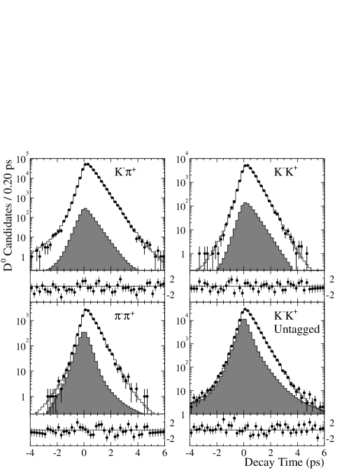
Figure 2: Decay time distributions for CF $D^{0}\!\rightarrow\!K^{-}\pi^{+}$ (upper left), $D^{0}\!\rightarrow\!K^{+}K^{-}$ (upper right), $D^{0}\!\rightarrow\!\pi^{+}\pi^{-}$ (lower left), and $D^{0}\!\rightarrow\!K^{+}K^{-}$ selected without using a $D^{*\,+}$ tag (lower right), from BaBar using 91 fb^-1 of data.[8] The shaded histograms show the signal component obtained from the fit; residuals from the fit are plotted below each distribution.

4 $D^{0}(t)\!\rightarrow\!K^{+}\pi^{-}$ Doubly-Cabibbo-Suppressed Decays

For $D^{0}\!\rightarrow\!K^{+}\pi^{-}\!$, ${\cal A}_{f}$ is DCS, $\bar{\cal A}_{f}$ is CF, and thus $|{\cal A}_{f}|\!\!\ll\!\!|\bar{\cal A}_{f}|$. In addition, there may be a strong phase difference ($\delta$) between the amplitudes. Defining $R_{D}\!\equiv\!|{\cal A}_{f}/\bar{\cal A}_{f}|^{2}$ and $\overline{R}_{D}\!\equiv\!|\bar{\cal A}_{\bar{f}}/{\cal A}_{\bar{f}}|^{2}$, $\lambda\!=\!|q/p|\,R^{\,-1/2}_{D}\,e^{i(\phi+\delta)}$ and $\bar{\lambda}\!=\!|p/q|\,\overline{R}^{\,-1/2}_{D}\,e^{i(-\phi+\delta)}$. Inserting these terms into Eqs. (1) and (2) gives

$$\hskip-21.68121ptR(D^{0}\!\rightarrow\!K^{+}\pi^{-})\!\!\! \propto\!\!\!$$ (6)

$$\hskip-79.49744pte^{-\overline{\Gamma}t}\left[R_{D}+\left|\frac{q}{p}\right|\sqrt{R_{D}}\left[y^{\prime}\cos\phi-x^{\prime}\sin\phi\right](\overline{\Gamma}t)+\left|\frac{q}{p}\right|^{2}\frac{(x^{\prime 2}+y^{\prime 2})}{4}(\overline{\Gamma}t)^{2}\right]$$

$$\hskip-21.68121ptR(\overline{D}{}^{\,0}\!\rightarrow\!K^{-}\pi^{+})\!\!\! \propto\!\!\!$$ (7)

$$\hskip-79.49744pte^{-\overline{\Gamma}t}\left[\overline{R}_{D}+\left|\frac{p}{q}\right|\sqrt{\overline{R}_{D}}\left[y^{\prime}\cos\phi+x^{\prime}\sin\phi\right](\overline{\Gamma}t)+\left|\frac{p}{q}\right|^{2}\frac{(x^{\prime 2}+y^{\prime 2})}{4}(\overline{\Gamma}t)^{2}\right]\,,$$

where $x^{\prime}\!\equiv\!x\cos\delta+y\sin\delta$ and $y^{\prime}\!\equiv\!-x\sin\delta+y\cos\delta$. These “rotated” mixing parameters absorb the unknown strong phase difference $\delta$. $CPV$ enters Eqs. (6) and (7) in three ways: $|q/p|\neq 1$ ($CPV$ in mixing), $R_{D}\neq\overline{R}_{D}$ ($CPV$ in the DCS amplitude), and $\phi\neq 0$ ($CPV$ via interference between the DCS and mixed amplitudes). Assuming no $CPV$ gives the simpler expression

$$R\!\!\! \propto\!\!\! e^{-\overline{\Gamma}t}\left[R_{D}+\sqrt{R_{D}}\,y^{\prime}(\overline{\Gamma}t)+\frac{(x^{\prime 2}+y^{\prime 2})}{4}(\overline{\Gamma}t)^{2}\right]\,.$$ (8)

To date, six experiments[10, 11, 12] have done a time-dependent analysis of $D^{0}\!\rightarrow\!K^{+}\pi^{-}$ decays; the most stringent constraints on $x^{\prime 2}$ and $y^{\prime}$ are from Belle using 400 fb^-1 of data.[12] The reconstructed $M_{K\pi}$ and $Q$ distributions after all selection criteria are shown in Fig. 3; fitting these distributions yields $1073993\,\pm 1108$ RS signal events and $4024\,\pm 88$ WS signal events. Those events satisfying $|M_{K\pi}\!-M_{D^{0}}|<22$ MeV/$c^{2}$ and $|Q-5.8~{}{\rm MeV}|<1.5$ MeV ($4\sigma$ intervals) have their decay times fitted for $x^{\prime 2},\,y^{\prime}$, and $R_{D}$. The results are listed in Table 1; projections of the fit are shown in Fig. 4(left).

Table 1: Limits on mixing parameters obtained from fitting the decay time distribution of WS $D^{0}\!\rightarrow\!K^{+}\pi^{-}$ decays, from Belle using 400 fb^-1 of data.[12]

Fit Case	Parameter	Fit Result	95% C.L. interval
		$(\times 10^{-3})$	$(\times 10^{-3})$
No $CPV$	$x^{\prime 2}$ $y^{\prime}$ $R_{D}$ $R_{M}$	$0.18\,^{+0.21}_{-0.23}$ $0.6\,^{+4.0}_{-3.9}$ $3.64\pm 0.17$ –	$<0.72$ $(-9.9,6.8)$ $(3.3,4.0)$ $(0.63\times\!10^{-5},\,0.40)$
$CPV$ allowed	$x^{\prime 2}$ $y^{\prime}$ $R_{M}$ $A_{D}$ $A_{M}$	– – – $23\,\pm 47$ $670\,\pm 1200$	$<0.72$ $(-28,21)$ $<0.40$ $(-76,107)$ $(-995,1000)$
No mixing/$CPV$	$R_{D}$	$3.77\,\pm 0.08\,({\rm stat})\,\pm 0.05\,({\rm syst})$

A 95% C.L. region in the $x^{\prime 2}$-$y^{\prime}$ plane is obtained using a frequentist technique based on “toy” Monte Carlo (MC) simulation. For points $\vec{\alpha}=(x^{\prime 2},\,y^{\prime})$, one generates ensembles of MC experiments and fits them using the same procedure as that used for the data. For each experiment, the difference in likelihood $\Delta L\equiv\ln L_{\rm max}\!-\ln L(\vec{\alpha})$ is calculated, where $L_{\rm max}$ is evaluated for $x^{\prime 2}\geq 0$. The locus of points $\vec{\alpha}$ for which 95% of the ensemble has $\Delta L$ less than that of the data is taken as the 95% C.L. contour. This contour is shown in Fig. 4(right); projections of the contour are listed in the right-most column of Table 1.

$CPV$ is accounted for by fitting the $D^{0}\!\rightarrow\!K\pi$ and $\overline{D}{}^{\,0}\!\rightarrow\!K\pi$ samples separately; this yields six values: $x^{\prime 2\,\pm},\,y^{\prime\pm}$, and $R^{\pm}_{D}$. Defining $R^{\pm}_{M}\!\equiv\!(x^{\prime\pm\,2}+y^{\prime\pm\,2})/2$ and $A_{M}\!\equiv\!(R^{+}_{M}-R^{-}_{M})/(R^{+}_{M}+R^{-}_{M})$, one finds

$$x^{\prime\pm} = \left(\frac{1\pm A_{M}}{1\mp A_{M}}\right)^{1/4}(x^{\prime}\cos\phi\ \pm\ y^{\prime}\sin\phi)$$ (9)

$$y^{\prime\pm} = \left(\frac{1\pm A_{M}}{1\mp A_{M}}\right)^{1/4}(y^{\prime}\cos\phi\ \mp\ x^{\prime}\sin\phi)\,,$$ (10)

where there is an implicit sign ambiguity in $x^{\prime\pm}$ due to Eqs. (6) and (7) being quadratic in $x^{\prime}$. To allow for $CPV$, one obtains separate $1\!-\!\sqrt{0.05}\!=\!77.6\%$ C.L. contours for $(x^{\prime+\,2},\,y^{\prime+})$ and $(x^{\prime-\,2},\,y^{\prime-})$; points on the $(x^{\prime+\,2},\,y^{\prime+})$ contour are then combined with points on the $(x^{\prime-\,2},\,y^{\prime-})$ contour and the combination used to solve Eqs. (9) and (10) for $x^{\prime 2}$ and $y^{\prime}$. Because the relative sign of $x^{\prime+}$ and $x^{\prime-}$ is unknown, there are two solutions (one for each sign); Belle plots both in the $(x^{\prime 2},\,y^{\prime})$ plane and takes the outermost envelope of points as the 95% C.L. contour allowing for $CPV$. This contour has a complicated shape [see Fig. 4(right)] due to the two solutions. Projections of the contour are listed in the right-most column of Table 1. In the case of no $CPV$, the no-mixing point $x^{\prime 2}=y^{\prime}=0$ lies just outside the 95% C.L. contour; this point corresponds to 3.9% C.L. with systematic uncertainty included.

     

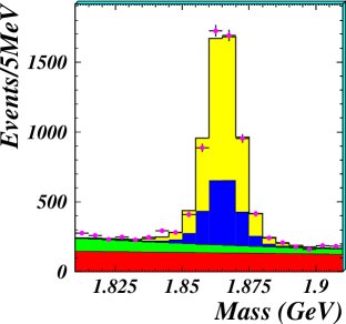
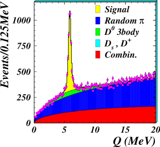
Figure 3: WS $D^{0}\!\rightarrow\!K^{+}\pi^{-}$ decays: $M_{K\pi}$ spectrum for events satisfying $Q\!\in(5.3,\,6.5)$ MeV (left), and $Q$ spectrum for events satisfying $M_{K\pi}\!\in(1.845,\,1.885)$ GeV/$c^{2}$, from Belle using 400 fb^-1 of data.[12]

Figure 4: Left: WS $D^{0}\!\rightarrow\!K^{+}\pi^{-}$ decay-time distribution and fit projections. Right: 95% C.L. region for $x^{\prime 2}$, $y^{\prime}$. From Belle using 400 fb^-1 of data.[12].

5 $D^{0}(t)\!\rightarrow\!K^{0}_{S}\,\pi^{+}\pi^{-}$ Dalitz Plot Analysis

In this method one considers a self-conjugate final state that is not a $CP$ eigenstate, e.g., a three-body decay that can have either $L\!=\!0$ ($CP$-even) or $L\!=\!1$ ($CP$-odd). If $CPV$ is negligible, $CP$-eigenstates (denoted $D_{-},\,D_{+}$) are mass eigenstates (denoted $D_{1},\,D_{2}$), and the amplitude for $D^{0}(t)\!\rightarrow\!K^{0}_{S}\,\pi^{+}\pi^{-}$ is:

$${\cal A}_{K^{0}\pi\pi}\!\!\! =\!\!\! \frac{1}{2p}\Big{(}\langle K^{0}_{S}\,\pi^{+}\pi^{-}|H|D_{-}(t)\rangle\ +\ \langle K^{0}_{S}\,\pi^{+}\pi^{-}|H|D_{+}(t)\rangle\Big{)}$$ (11)

$$\equiv {\cal A}_{-}\,e^{-(\Gamma_{1}/2+im_{1})\,t}\ +\ {\cal A}_{+}\,e^{-(\Gamma_{2}/2+im_{2})\,t}$$

$$\hskip-28.90755pt\Rightarrow\ R_{K^{0}\pi\pi}\!\!\! =\!\!\! |{\cal A}_{-}|^{2}\,e^{-\overline{\Gamma}(1-y)t}\ +\ |{\cal A}_{+}|^{2}\,e^{-\overline{\Gamma}(1+y)t}\ +\$$ (12)

$$2e^{-\overline{\Gamma}t}\left[\,{\rm Re}({\cal A}_{+}\,{\cal A}^{*}_{-})\cos(\Delta m\,t)+{\rm Im}({\cal A}_{+}\,{\cal A}^{*}_{-})\sin(\Delta m\,t)\,\right],$$

where ${\cal A}_{+,-}$ is the amplitude for $D_{+,-}\!\!\rightarrow\!K^{0}_{S}\,\pi^{+}\pi^{-}$ multiplied by $1/(2p)$. Note that $x\!=\!(m_{2}-m_{1})/\overline{\Gamma}$ and $y\!=\!(\Gamma_{2}-\Gamma_{1})/(2\overline{\Gamma})$. For a three-body final state, one can distinguish the ${\cal A}_{+}$ and ${\cal A}_{-}$ components via a Dalitz plot analysis; i.e., a $K^{0}_{S}\,f_{0}(980)$ intermediate state is $CP$-even and contributes to ${\cal A}_{+}$, $K^{0}_{S}\,\rho^{0}$ is $CP$-odd and contributes to ${\cal A}_{-}$, $K^{*}(890)^{+}\,\pi^{-}$ is a flavor-eigenstate and contributes to both ${\cal A}_{+}$ and ${\cal A}_{-}$, etc. Thus one models ${\cal A}_{+,-}$ by separate sums of amplitudes $\sum_{j}a_{j}\,e^{i\delta_{j}}A_{j}$, where $A_{j}$ is the Breit-Wigner amplitude[13] for resonance $j$ and is a function of the Dalitz plot position $M^{2}_{K^{0}\pi^{+}}$, $M^{2}_{K^{0}\pi^{-}}$. Using the probability density function of Eq. (12), one does an unbinned maximum likelihood fit to $M^{2}_{K^{0}\pi^{+}}$, $M^{2}_{K^{0}\pi^{-}}$, and the decay time $t$ to determine $a_{j}$, $\delta_{j}$, $x$, and $y$. There is systematic uncertainty arising from the decay model, i.e., one must decide which intermediate states to include in the fit. Unlike Eq. (6), Eq. (12) depends linearly on $x$ ($x\!\ll\!1$) and is therefore sensitive to its sign.

This analysis was developed by CLEO, and their result[14] based on 9.0 fb^-1 has not yet been superseded. To minimize backgrounds, the $D^{0}$ candidate is required to originate from $D^{*\,+}\!\rightarrow\!D^{0}\pi^{+}$. The final Dalitz plot sample (Fig. 5) contains 5299 events with only $(2.1\,\pm 1.5)$% background.[15]

The decay model used consists of $D^{0}\!\rightarrow\!K^{*}(890)^{-}\,\pi^{+}\!$, $K^{*}(1430)^{-}_{0,2}\,\pi^{+}\!$, $K^{*}(1680)^{-}\,\pi^{+}\!$, $K^{0}_{S}\,\rho$, $K^{0}_{S}\,\omega$, $K^{0}_{S}\,f_{0}(980)$, $K^{0}_{S}\,f_{2}(1270)$, $K^{0}_{S}\,f_{0}(1370)$, WS $D^{0}\!\rightarrow\!K^{*}(890)^{+}\,\pi^{-}\!$, and a nonresonant component. The fit results are listed in Table 2; the 95% C.L. intervals correspond to the values at which $-2\ln{\cal L}$ rises by 3.84 units, where ${\cal L}$ is the likelihood function. $CPV$ is included in the fit by introducing parameters $\varepsilon\equiv(p-q)/(p+q)$ (in analogy with $K^{0}$ decays) and $\phi$, the weak phase difference between $\bar{\cal A}_{K^{0}\pi\pi}$ and ${\cal A}_{K^{0}\pi\pi}$. The results listed are consistent with no mixing or $CPV$.

Figure 5: Dalitz plot (lower right) and projections (lower left, upper plots) for $D^{0}\!\rightarrow\!K^{0}_{S}\,\pi^{+}\pi^{-}$ decays, from CLEO using 9.0 fb^-1 of data.[15]

Table 2: Limits on mixing and $CPV$ parameters from a $t$-dependent fit to the $D^{0}\!\rightarrow\!K^{0}_{S}\,\pi^{+}\pi^{-}$ Dalitz plot, from CLEO using 9.0 fb^-1.[14] The errors are statistical, experimental systematic, and modeling systematic, respectively.

Fit	Param.	Fit Result (%)	95% C.L. Inter. (%)
No $CPV$	$x$ $y$	$1.8\,^{+3.4}_{-3.2}\,\pm 0.4\,\pm 0.4$ $-1.4\,^{+2.5}_{-2.4}\,\pm 0.8\,\pm 0.4$	$(-4.7,8.6)$ $(-6.3,3.7)$
$CPV$   Allowed	$x$ $y$ $\epsilon$ $\phi$	$2.3\,^{+3.5}_{-3.4}\,\pm 0.4\,\pm 0.4$ $-1.5\,^{+2.5}_{-2.4}\,\pm 0.8\,\pm 0.4$ $1.1\,\pm 0.7\,\pm 0.4\,\pm 0.2$ $(5.7\,\pm 2.8\,\pm 0.4\,\pm 1.2)^{\circ}$	$(-4.5,9.3)$ $(-6.4,3.6)$ $(-0.4,2.4)$ $(-0.3^{\circ},11.7^{\circ})$

6 $D^{0}(t)\!\rightarrow\!K^{+}\pi^{-}\pi^{0}$ and $K^{+}\pi^{-}\pi^{+}\pi^{-}$ Multibody Decays

Mixing has also been searched for in WS multibody final states[10, 16, 17] $K^{+}\pi^{-}\pi^{0}$ and $K^{+}\pi^{-}\pi^{+}\pi^{-}$; the most recent measurement is from Belle using 281 fb^-1 of data.[17] The final signal yields are $1978\pm 104$ $D^{0}\!\rightarrow\!K^{+}\pi^{-}\pi^{0}$ decays and $1721\pm 75$ $D^{0}\!\rightarrow\!K^{+}\pi^{-}\pi^{+}\pi^{-}$ decays. For this analysis no decay time information is used, i.e., Belle measures the time-integrated ratio of WS to RS decays:

$$R_{\rm WS}\!\!\! =\!\!\! \frac{\int R[D^{0}\!\rightarrow\!K^{+}\pi^{-}(n\pi)]\,dt}{\int R[D^{0}\!\rightarrow\!K^{-}\pi^{+}(n\pi)]\,dt}\ \approx\ R_{D}+\sqrt{R_{D}}\,y^{\prime}+\frac{x^{\prime 2}+y^{\prime 2}}{2}\,,$$ (13)

where $R_{D}$ is the ratio of the DCS rate to the CF rate as previously defined for $D^{0}\!\rightarrow\!K^{+}\pi^{-}$ decays. The results are $R_{\rm WS}=[0.229\,\pm 0.015\,({\rm stat})\,^{+0.013}_{-0.009}\,({\rm syst})]$% for $K^{+}\pi^{-}\pi^{0}$ and $[0.320\,\pm 0.018\,({\rm stat})\,^{+0.018}_{-0.013}\,({\rm syst})]$% for $K^{+}\pi^{-}\pi^{+}\pi^{-}$. Inserting these values into Eq. (13) allows one to determine $R_{D}$ as a function of $x^{\prime}$ or $y^{\prime}$. Assuming $x^{\prime}\!=\!0$ and $|x^{\prime}|\!=\!0.027$ gives the curves shown in Fig. 6; the latter $|x^{\prime}|$ value corresponds to Belle’s 95% C.L. upper limit from $D^{0}\!\rightarrow\!K^{+}\pi^{-}$ decays (see Table 1). However, the value of $x^{\prime}$ from $D^{0}\!\rightarrow\!K^{+}\pi^{-}$ may differ from that from $D^{0}\!\rightarrow\!K^{+}\pi^{-}n(\pi)$ due to the strong phase differences ($\delta$) being different.

Figure 6: WS $D^{0}\!\rightarrow\!K^{+}\pi^{-}n(\pi)$ decays: 95% C.L. range for $R_{D}$ as a function of $y^{\prime}$ for $|x^{\prime}|=0$ and $|x^{\prime}|=0.027$, from Belle using 281 fb^-1 of data.[17] The point with $1\sigma$ error bars is Belle’s result from $D^{0}\!\rightarrow\!K^{+}\pi^{-}$ decays (see Table 1).

7 Summary

The 95% C.L. allowed ranges for $x^{\prime}$ and $y^{\prime}$ are plotted in Fig. 7; for simplicity we assume negligible $CPV$. The most stringent constraints are $|x^{\prime}|\!<\!2.7$% and $y^{\prime}\!\in(-1.0\%,\,0.7\%)$. These ranges are projections of the two-dimensional 95% C.L. region for $x^{\prime 2},\,y^{\prime}$ from Belle [Fig. 4(right)].

The results for $y_{CP}$ are plotted in Fig. 8. Here the central values and $1\sigma$ errors are shown; combining the results assuming the errors uncorrelated gives $y_{CP}\!=\!(1.09\,\pm 0.46)$%. This value differs from zero by $2.4\sigma$ and indicates a nonzero decay width difference $\Delta\Gamma$. Assuming negligible $CPV$, one can combine this value with Belle’s central value for $y^{\prime}$, $(0.06\,^{+0.40}_{-0.39})\%$. The result is $y^{\prime}/y=\cos\delta-(x/y)\sin\delta=0.05\,^{+0.39}_{-0.37}$, where the error is obtained from an MC calculation as the fractional errors on $y$ and $y^{\prime}$ are large. This small central value (albeit with a large error) implies $\tan\delta\approx y/x$; i.e., if $x\!\ll\!y$, then $\delta$ is near 90^∘. Such a strong phase difference would be much larger than expected.

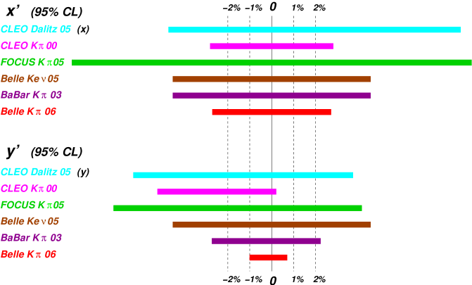
Figure 7: 95% C.L. allowed ranges for $x^{\prime}$ (top) and $y^{\prime}$ (bottom) from various experiments assuming no $CPV$. The CLEO Dalitz results are for $x$ and $y$.

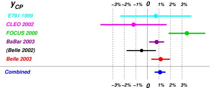
Figure 8: $y_{CP}$ central values and $1\sigma$ errors measured by various experiments, and the combined result assuming the individual errors uncorrelated. The Belle 2002 data sample (23 fb^-1) has some overlap with the Belle 2003 data sample (158 fb^-1), and thus this result is not included in the average.

References

- 1 . Z.-Z. Xing, Phys. Rev. D 55, 196 (1997).
- 2 . S. Bianco, F. L. Fabbri, D. Benson, and I. Bigi, Riv. Nuovo Cim. 26N7-8, 1 (2003).
- 3 . A. A. Petrov, Charm physics: theoretical review, in: Proc. of the Second International Conference on Violation and Flavor Physics (ed. P. Perret, Ecole Polytechnique, Paris, June 2003), eConf C030603, hep-ph/0311371. See also: A. A. Petrov, hep-ph/0409130 (2004).
- 4 . D. M. Asner and W. M. Sun, Phys. Rev. D 73, 034024 (2006).
- 5 . E. M. Aitala et al. (FNAL E791), Phys. Rev. Lett. 77, 2384 (1996). B. Aubert et al. (BaBar), Phys. Rev. D 70, 091102 (2004). C. Cawlfield et al. (CLEO), Phys. Rev. D 71, 077101 (2005).
- 6 . U. Bitenc et al. (Belle), Phys. Rev. D 72, 071101(R) (2005).
- 7 . E. M. Aitala et al. (FNAL E791), Phys. Rev. Lett. 83, 32 (1999). S. E. Csorna et al. (CLEO), Phys. Rev. D 65, 092001 (2002). K. Abe et al. (Belle), BELLE-CONF-347, hep-ex/0308034 (2003); Phys. Rev. Lett. 88, 162001 (2002).
- 8 . B. Aubert et al. (BaBar), Phys. Rev. Lett. 91, 121801 (2003).
- 9 . J. M. Link et al. (FOCUS), Phys. Lett. B 485, 62 (2000).
- 10 . E. M. Aitala et al. (FNAL E791), Phys. Rev. D 57, 13 (1998).
- 11 . R. Barate et al. (ALEPH), Phys. Lett. B 436, 211 (1998). R. Godang et al. (CLEO), Phys. Rev. Lett. 84, 5038 (2000). J. M. Link et al. (FOCUS), Phys. Lett. B 618, 23 (2005); Phys. Rev. Lett. 86, 2955 (2001). B. Aubert et al. (BaBar), Phys. Rev. Lett. 91, 171801 (2003).
- 12 . L. Zhang et al. (Belle), Phys. Rev. Lett. 96, 151801 (2006); J. Li et al. (Belle), Phys. Rev. Lett. 94, 071801 (2005).
- 13 . S. Kopp et al. (CLEO), Phys. Rev. D 63, 092001 (2001).
- 14 . D. M. Asner et al. (CLEO), Phys. Rev. D 72, 012001 (2005).
- 15 . H. Muramatsu et al. (CLEO), Phys. Rev. Lett. 89, 251802 (2002).
- 16 . G. Brandenburg et al. (CLEO), Phys. Rev. Lett. 87, 071802 (2001). S. A. Dytman et al. (CLEO), Phys. Rev. D 64, 111101 (2001).
- 17 . X. C. Tian et al. (Belle), Phys. Rev. Lett. 95, 231801 (2005).