Recent results on fully leptonic and semileptonic charm decays

Abstract

We begin with giving some motivation for the study of charm semileptonic and fully leptonic decays. We turn next to a discussion of semileptonic absolution branching fraction results form CLEO-c. Two exciting high statistics results on fully leptonic decays of the $D^{+}\rightarrow\mu^{+}\nu$ and $D_{s}^{+}\rightarrow\mu^{+}\nu$ from CLEO-c and BaBar are reviewed. We turn next to a discussion of recent results on charm meson decay to pseudo-scalar $\ell nu$ decays from FOCUS, BaBar, and CLEO-c. We conclude with a review of charm meson decay into Vector $\ell\nu$ .

I Introduction

Figure 1 shows cartoons of the $D_{s}^{+}\rightarrow\ell^{+}\nu$ fully leptonic process and the $D^{0}\rightarrow K^{-}\ell^{+}\nu$ semileptonic decay process. All of the hadronic complications for this process are contained in the decay constant for fully leptonic decay or the $q^{2}{}$ dependent form factor for semileptonic processes. Both are computable using non-perturbative methods such as LQCD. Although both processes can in principle provide a determination of charm CKM elements, one frequently uses the (unitarity constrained) CKM measurements, lifetime, and branching fraction to measure the $f_{D}$ decay constant or the $q^{2}$ integral of the square of the semileptonic form factor. These can then be compared to LQCD predictions to provide an incisive test of this technique. The $q^{2}{}$ dependence of the semileptonic form factor can also be directly measured and compared to theoretical predictions.

The hope is that charm semileptonic and fully leptonic decays can provide high statistics, precise tests of LQCD calculations and thus validate the computational techniques for charm. Once validated, the same LQCD techniques can be used in related calculations for $B$-decay and thus produce CKM parameters with significantly reduced theory systematics. For example the recent $B_{s}^{0}$ mixing rate measurement by CDF and D0 is proportional to the squared $f_{B_{s}}$ decay constant. The analogous $f_{D_{s}}$ computed using similar methods was recently measured by the BaBar Collaboration.

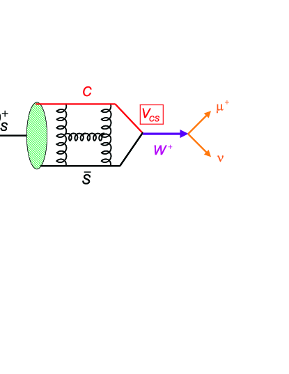
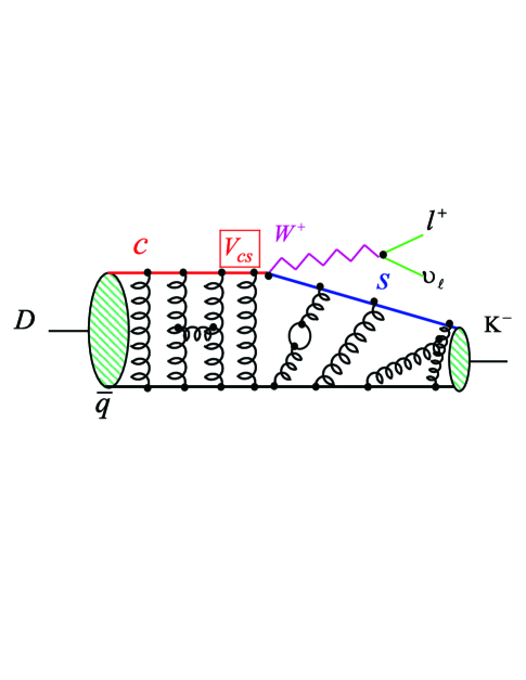
Figure 1: Diagrams for the fully leptonic (top) and semileptonic (bottom) decay of charmed mesons. The QCD complications are contained in a decay constant $f_{D}$ for the fully leptonic case, and $q^{2}$ dependent form factors for semileptonic decays. Both processes, in principle, provide measurements of CKM matrix elements

II Absolute Semileptonic Decay Branching Fractions from CLEO

These results are based on the first 56 pb^-1 of CLEO charm threshold running at the $\psi(3770)$ At this energy charm is produced by either in $D^{0}\bar{D}^{0}$ or $D^{+}D^{-}$ final states since there is not enough kinematic room to produce an additional pion dtag . This is a particularly desirable environment for measuring absolute branching fractions since one essentially divides the corrected number of observed $DX$ events where $X$ decays into a given semileptonic state to the total corrected number of states with a reconstructed D. The semileptonic branching fraction results cleobr are summarized in Fig. 2.

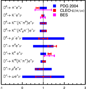
Figure 2: Ten exclusive absolute semileptonic branching fractions measured by the CLEO collaboration divided by the previous world average values compiled by PDG2004. The CLEO fractional errors are shown with red error bars within the blue boxes. The PDG2004 relative errors are shown as blue boxes. Even though these results are based on only about 20% of CLEO’s present sample, in most cases they are more precise than the previous world average.

Figure 3 gives an example of the CLEO $D^{0}\rightarrow\pi^{-}e^{+}\nu$ signal. The signal appears as a peak centered at zero in the variable $U\equiv E_{\rm Miss}-c|\vec{P}_{\rm Miss}|$ in events with a fully reconstructed ${\bar{D}}^{0}$. To get a contribution to the signal peak, one must have a single missing $\nu$ and the proper masses must be assigned to the charged semileptonic decay daughters in constructing $E_{\rm Miss}$. Figure 3 illustrates the power of this kinematic constraint by showing the separation between the $D^{0}\rightarrow\pi^{-}e^{+}\nu$ signal and a $D^{0}\rightarrow K^{-}e^{+}\nu$ background where the $K^{-}$ has been misidentified a $\pi^{-}$ by the particle identification system. Even though the $K^{-}e^{+}\nu$ dominates over $\pi^{-}e^{+}\nu$ by about an order of magnitude, its contamination near $U\approx 0$ is very small and manageable.

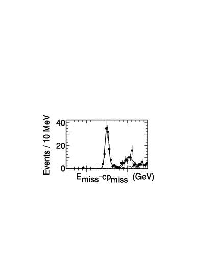
Figure 3: Illustration of a $\pi^{+}e^{+}\nu$ signal obtained in the first 57 pb^-1 of CLEO-c running at the $\psi(3770)$. The signal forms a peak near $U\equiv E_{\rm Miss}-c|\vec{P}_{\rm Miss}|\approx 0$. A misidentification background from $D^{0}\rightarrow K^{-}e^{+}\nu$ is well displaced from the signal.

CLEO has also reported on inclusive semileptonic decays of the $D^{0}$ and the $D^{+}$. The data are based 281 pb^-1 of their $\psi(3770)$ running. Figure 4 compares the electronic momentum spectrum obtained against tagged $D^{0}$ and the $D^{+}$ along the curves used to extrapolate the spectrum below their cut-off of $P_{e}<~{}200~{}MeV/c$. Roughly 7.6% of the semileptonic decays produce an electron below this $200~{}MeV$ electron momentum cut according to their Monte Carlo model generated with ISGW2 form factors. A 1% systematic uncertainty is assessed on the inclusive $\mathcal{B}$ values summarized in Table 1 for the momentum extrapolation below 200 MeV/$c$.

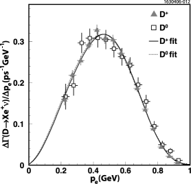
Figure 4: The momentum spectrum of electrons/positrons for the CLEO-c inclusive semileptonic selection for $D^{0}$ and $D^{+}$ candidates. The fitted curves, based a Monte Carlo model, are used to extrapolate the spectrum below the electron momentum cut-off of 200 MeV$/c$.

The table summarizes the preliminary results for the $D^{0}$ and $D^{+}$ inclusive semileptonic branching fractions and compares each result to the sum of the CLEO exclusive mode branching fractions. The known exclusive modes come close to saturating the inclusive modes although there might be some room for additional, unmeasured exclusive states.

Table 1: Inclusive semileptonic branching fractions compared to the sum of the semi exclusive branching fractions measured by CLEO.

$D^{0}\rightarrow Xe^{+}\nu$	(6.46 $\pm$ 0.17 $\pm$ 0.13)%
$\Sigma_{i}\mathcal{B}_{i}\left(D^{0}\rightarrow Xe^{+}\nu\right)$	(6.1 $\pm$ 0.2 $\pm$ 0.2)%
$D^{+}\rightarrow Xe^{+}\nu$	(16.13 $\pm$ 0.20 $\pm$ 0.33)%
$\Sigma_{i}\mathcal{B}_{i}\left(D^{+}\rightarrow Xe^{+}\nu\right)$	(15.1 $\pm$ 0.5 $\pm$ 0.5)%

One can also use the ratio of the exclusive $D^{+}$ and $D^{0}$ semileptonic branching fractions and the known $D^{0}$ and $D^{+}$ lifetimes to measure the ratio of $D^{+}$ and $D^{0}$ semileptonic widths.

$${\frac{{\Gamma_{D^{+}}^{SL}}}{{\Gamma_{D^{0}}^{SL}}}=\frac{{B_{D^{+}}^{SL}}}{{B_{D^{0}}^{SL}}}\times\frac{{\tau_{D^{0}}}}{{\tau_{D^{+}}}}\;=0.985\pm 0.028\pm 0.015}$$ (1)

The value is consistent with unity as expected from isospin symmetry. The errors on the new CLEO width ratio represents a considerable improvement over previous data.

III Fully leptonic decays from CLEO and BaBar

Charm fully leptonic decays are difficult to study because of their very low branching ratios. The rate is low since the charged lepton is forced into an unnatural helicity state to conserve angular momentum. The decay width is proportional to two powers of the lepton mass – in this case the mass of the muon.

$$B(D\to\mu\nu)/\tau_{D}=\frac{{G_{F}^{2}}}{{8\pi}}f_{D}^{2}m_{\mu}^{2}M_{D}\left({1-\frac{{m_{\mu}^{2}}}{{M_{D}^{2}}}}\right)\left|{V_{cq}}\right|^{2}{\rm{}}$$ (2)

For example CLEO fdpls measures $\mathcal{B}\left(D^{+}\rightarrow\mu^{+}\nu\right)=(4.40\pm 0.66\pm 0.1)\times 10^{-4}$ , while BaBar has a preliminary measurement of $\mathcal{B}\left(D_{s}^{+}\rightarrow\mu^{+}\nu\right)=(6.5\pm 0.8\pm 0.3\pm 0.9)\times 10^{-3}$. The order of magnitude larger $D_{s}^{+}\rightarrow\mu^{+}\nu$ fully leptonic $\mathcal{B}$ reflects the factor-of-two difference in the $D_{s}^{+}$ and $D^{+}$ lifetimes as well as the fact that the $D_{s}^{+}$ fully leptonic decay is a Cabibbo favored process where $D^{+}\rightarrow\mu^{+}\nu$ is not.

Both the CLEO signal for $D^{+}\rightarrow\mu^{+}\nu$ ($\approx 50$ signal events) and the preliminary BaBar signal for $D_{s}^{+}\rightarrow\mu^{+}\nu$ ($489\pm 55$ signal events) are shown in Fig. 5.

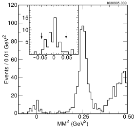
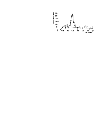
Figure 5: Signals for $D^{+}\rightarrow\mu^{+}\nu$ from CLEO (top) and $D_{s}^{+}\rightarrow\mu^{+}\nu$ from BaBar (bottom). The $D^{+}\rightarrow\mu^{+}\nu$ signal appears as a peak in the missing mass distributions in CLEO tagged events where all tracks are reconstructed but the neutrino. The $D_{s}^{+}\rightarrow\mu^{+}\nu$ signal forms a peak in the $D_{s}^{+*}\rightarrow\gamma D_{s}^{+}$ mass difference plot.

The CLEO signal, based 281 pb^-1 of the $\psi(3770)$ running, is a peak near zero in the missing-mass in events where there is a single track recoiling against a fully reconstructed $D^{-}$. The prominent peak centered to the right of the neutrino peak, near a missing mass of $\approx 0.25~{}\rm{GeV}^{2}/c^{2}$, presumably corresponds to charm decays with an unreconstructed $K_{L}$.

The BaBar analysis is very different since they are running at the $\Upsilon(4S)$ which is far from charm threshold. They observe the $D_{s}^{+}\rightarrow\mu^{+}\nu$ decay by observing a peak in the $\Delta m\equiv m(\mu^{+}\nu~{}\gamma)-m(\mu^{+}\nu)$ mass difference corresponding to the decay $D_{s}^{+*}\rightarrow\gamma D_{s}^{+}$. The neutrino four-vector is estimated from the missing momentum in the event along with the application of a $D_{s}^{+}$ mass constraint when the neutrino is combined with the reconstructed muon. There is a slight peaking background near $\approx 0.07~{}\rm{GeV}/c$ due to photons originating from $\pi^{0}$ rather than $D_{s}^{+*}$ decay. The dashed background is due to $D_{s}^{+*}\rightarrow\gamma D_{s}^{+}\rightarrow\gamma(\tau^{-}\nu)$ decays. It is interesting to note that although the $D^{+*}\rightarrow\gamma D^{+}\rightarrow\gamma(\mu^{+}\nu)$ background will peak at essentially the same $\Delta m$ as the $D_{s}^{+*}\rightarrow\gamma D_{s}^{+}\rightarrow\gamma(\mu^{+}\nu)$ signal, this background will be essentially negligible in light of the order of magnitude lower $\mathcal{B}\left(D^{+}\rightarrow\mu^{+}\nu\right)$ and the fact that $\mathcal{B}\left(D_{s}^{+*}\rightarrow\gamma D_{s}^{+}\right)$ is about 60 $\times$ larger than $\mathcal{B}\left(D^{+*}\rightarrow\gamma D^{+}\right)$.

Table 2: Fully leptonic decay constants

$f_{D+}$ LQCD (FNAL/MILC)milc	201 $\pm$ 3 $\pm$17 MeV
$f_{D+}$ (CLEO)fdpls	222.6$\pm$16.7${}^{+2.8}_{-3.4}$ MeV
$f_{Ds}$ (BaBar)	279 $\pm$ 17 $\pm$ 6 $\pm$19 MeV
$f_{Ds}$/ $f_{D+}$ BaBar/CLEO	1.25 $\pm$ 0.14

The CLEO $f_{D+}$ result is consistent with the latest LQCD estimate from the FNAL/MILC collaborationmilc and has comparable errors. The BaBar $f_{Ds}$ result is about 25 % higher than $f_{D+}$ as expected in LQCD calculations. Both $f_{D}$ decay constants are measured to about 8 %. The major systematic error for the BaBar measurement is $\pm$ 19 MeV, due to the $13\%$ uncertainly in the $\mathcal{B}\left(D_{s}^{+}\rightarrow\phi\pi^{+}\right)$ measured by BaBar which was used to normalize their $D_{s}^{+}\rightarrow\mu^{+}\nu$ signal.

IV Pseudoscalar $\mathbf{\ell\nu}$ decays from FOCUS, BaBar, Belle, and CLEO

The below equation gives the expression for the differential decay width for $D\to P\ell\nu$ where P is a pseudoscalar meson.

$$\frac{{d\Gamma\left({D\to P\ell\nu}\right)}}{{dq^{2}}}=\frac{{G_{F}^{2}\left|{V_{cq}}\right|^{2}P_{P}^{3}}}{{24\pi^{3}}}\left\{{\left|{f_{+}(q^{2})}\right|^{2}+O(m_{l}^{2})}\right\}$$ (3)

The pseudoscalar semileptonic decay – in the limit of low charged lepton mass – is controlled by a single form factor $f_{+}(q^{2}{})$. An important motivation for studying pseudoscalar semileptonic decays is to compare the measured $f_{+}(q^{2}{})$ to the calculated $f_{+}(q^{2}{})$ using techniques such as LQCD. The $P_{P}^{3}$ factor (where $P_{P}$ is the momentum of the pseudoscalar in the $D$ rest frame) creates a strong peaking of $d\Gamma/dq^{2}{}$ at low $q^{2}$. Unfortunately the low $q^{2}$ region is where discrimination between different $f_{+}(q^{2}{})$ models is the poorest, and LQCD calculations are the most difficult. To the extent that $f_{+}(q^{2}{})$ calculations are trusted, a measurement of the pseudoscalar semileptonic decay widths can provide new measurements of the CKM matrix elements.

We begin discuss studies on the shape of $f_{+}(q^{2}{})$ for the decay $D^{0}\rightarrow K^{-}\ell^{+}\nu$. An early parameterization for $f_{+}(q^{2}{})$ used spectroscopic pole dominance. This is based on a dispersion relation obtained using Cauchy’s Theorem under the assumption that $f_{+}(q^{2}{})$ is an analytic, complex function as illustrated in Fig. 6 for $D^{0}\rightarrow K^{-}e^{+}\nu$.

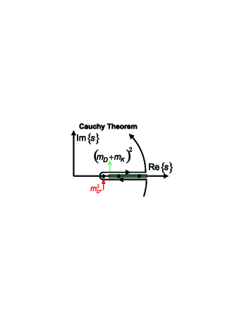
Figure 6: The form factor is assumed to be an analytic function with pole singularities at the masses of bound states, and cuts that start at the start of the continuum. One can use Cauchy’s theorem with the indicated contour to write an dispersion expression for $f_{+}(q^{2}{})$ in the physical range $0<q^{2}{}<\left(m_{D}-m_{K}\right)^{2}$.

The $f_{+}(q^{2}{})$ singularities will consist of simple poles at the $D^{0}K^{+}$ vector bound states (e.g. $D_{s}^{*+}$) and cuts beginning at the $D^{0}K^{+}$ continuum ($q^{2}{}>(M_{D}+M_{K})^{2}$). The dispersion relation gives $f_{+}(q^{2}{})$ as a sum of the spectroscopic pole and an integral over the cut:

$$f_{+}(q^{2})=\frac{\mathcal{R}}{{m_{D_{s}^{*}}^{2}-q^{2}}}+\frac{1}{\pi}\int_{\left({m_{D}+K}\right)^{2}}^{\infty}{\frac{{{\mathop{\rm Im}\nolimits}\left\{{f_{+}(s)}\right\}}}{{s-q^{2}-i\varepsilon}}ds}$$ (4)

Both the cuts and poles are beyond the physical $q^{2}{}_{\rm max}$ and thus can never be realized. One might expect the spectroscopic pole to dominate as $q^{2}{}\rightarrow m^{2}_{D_{s}*}$ as long as the pole were well separated from the cut. Neither of these conditions is particularly well satisfied for $D^{0}\rightarrow K^{-}e^{+}\nu$. The minimum separation from the pole is $\sqrt{q^{2}{}_{\rm max}}-m_{D_{s}*}=0.74~{}\rm{GeV}$ which seems large on the scale of the charm system. The gap between the pole and the start of the cut interval is only $0.25~{}\rm{GeV}$. Hence it does not appear that the data ever gets ”close’ to a ”well-isolated” pole in $D^{0}\rightarrow K^{-}e^{+}\nu$.

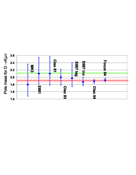
Figure 7: Effective pole mass measurement in $D^{0}\rightarrow K^{-}e^{+}\nu$ over the years mpole . The green line is the $m_{D_{S}^{*}}$ spectroscopic pole mass and is inconsistent with the average of the displayed data by 5.1 $\sigma$.

Several experiments have measured the ”effective” pole mass in $D^{0}\rightarrow K^{-}e^{+}\nu$ decay over the years, where ${\rm{f}}_{\rm{+}}(q^{2})\propto 1/{(m_{pole}^{2}-q^{2})}$. As Fig. 7 shows, as errors have improved over the years, it becomes clear that the effective pole is significantly lower than the spectroscopic pole, underscoring the importance of the cut integral contribution for this decay.

Becirevic and Kaidalov (1999) BK proposed a new parameterization for $f_{+}(q^{2}{})$ that would hopefully provide more insight into the interplay between the spectroscopic pole and the cut integral contributions.

$$f_{+}(q^{2})=\frac{{c_{D}m_{D*}^{2}}}{{m_{D*}^{2}-q^{2}}}-\frac{{\alpha\gamma c_{D}m_{D*}^{2}}}{{\gamma m_{D*}^{2}-q^{2}}}$$ (5)

Becirevic and Kaidalov represent the cut integral by an effective pole that is displaced from the spectroscopic pole by a factor of $\sqrt{\gamma}$, and has a residue that differs from the spectroscopic pole by a factor $-\alpha$. Becirevic and Kaidalov use counting laws, and form factor relations in the heavy quark limit to argue that $\alpha=1/\gamma$. This constraint leads to a modified pole form with a single additional parameter $\alpha$ that describes the degree to which the single spectroscopic pole fails to match $f_{+}(q^{2}{})$ for a given process.

$$f_{+}(q^{2})=\frac{{f_{+}(0)}}{{\left({1-q^{2}/m_{D*}^{2}}\right)\left({1-\alpha q^{2}/m_{D*}^{2}}\right)}}$$ (6)

The spectroscopic pole dominance limit is $\alpha\rightarrow 0$. As $\alpha$ is increased, the effective cut pole both gets closer to $q^{2}{}_{\rm max}$ limit while simultaneously acquiring a stronger residue. Both effects act to create a faster $q^{2}{}$ dependence than that of the spectroscopic pole thus creating an effective single effective pole with $m_{\rm pole}<m_{D_{s}*}$. This is indeed what happens in the data summarized in Fig. 7.

The Becirevic and Kaidalov parameterization has been used extensively in some of the calculational details of recent charm LQCD calculations of the $f_{+}$ form factor. The final $f_{+}(q^{2}{})$ computed in reference milc is well fit with a modified pole form with $\alpha(K^{-}e^{+}\nu)=0.5\pm 0.04$ and $\alpha(\pi^{-}e^{+}\nu)=0.44\pm 0.04$. It is interesting that the $\alpha$ parameters for the LQCD calculations $D^{0}\rightarrow\pi^{-}e^{+}\nu$ are so similar to those for $D^{0}\rightarrow K^{-}e^{+}\nu$ given the different locations of their singularities. For the $D^{0}\rightarrow\pi^{-}e^{+}\nu$, for example, $q^{2}{}_{\rm max}$ lies much closer to the spectroscopic pole than the case in $D^{0}\rightarrow K^{-}e^{+}\nu$ and for pion decay the $D^{*+}$ pole lies within the $D\pi$ continuum.

Although with present precision, data seems to match the modified pole form as well as the effective pole form, it is not clear that the heavy quark limit really applies to charm semileptonic decay. Alternative $f_{+}(q^{2})$ parameterizations have therefore been proposed in the literature Hill .

There are now several fine-bin, non-parametric measurements for $f_{+}(q^{2})$ for $D^{0}\rightarrow K^{-}e^{+}\nu$. Essentially the first of these was from FOCUS (2004). The FOCUS data uses the decay chain $D^{*+}\rightarrow\tilde{\pi}^{+}(K^{-}\mu^{+}\nu)$ and uses a signal consisting of $\approx 13000$ events after a tight $m(D^{*})-m(D)$ cut. Figure 8 illustrates the method used by FOCUS to reconstruct the missing neutrino required to compute $q^{2}$. In the $K^{-}-\mu^{+}$ center of frame, the requirement that $K^{-}\mu^{+}\nu$ forms a $D^{0}$ determines the energy of the $\nu$. The requirement that the $\tilde{\pi}^{+}(K^{-}\mu^{+}\nu)$ forms a $D^{+*}$ restricts the neutrino to lie on a cone about the $\tilde{\pi}$ momentum. The $D^{0}$ momentum vector is directed against the neutrino in this frame. One then varies the azimuth about the neutrino cone, boosts the $D^{0}$ momentum vector into the lab, and selects the azimuth where the $D^{0}$ comes closest to the primary vertex in the photoproduced event. The resultant $q^{2}$ resolution (also in Fig. 8 )is roughly $\sigma(q^{2}{})\approx 0.20~{}\rm{GeV}^{2}$ which is comparable to the $q^{2}$ binning of 0.18 GeV². A matrix based deconvolution technique is applied to the data. The adjacent $f_{+}(q^{2}{})$ values have roughly a 65% negative correlation owing to $q^{2}$ smearing between bins.

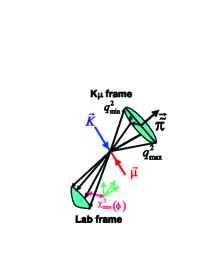
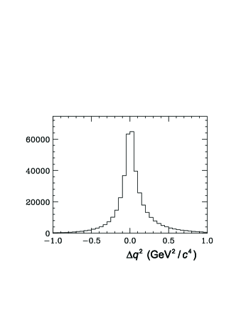
Figure 8: Illustration of how the neutrino can be reconstructed in a fixed target experiment such as FOCUS for the decay sequence $D^{*+}\rightarrow\tilde{\pi}^{+}(K^{-}\mu^{+}\nu)$ . In the $K^{-}\mu^{+}$ rest frame the neutrino lies on a cone with a momentum and 1/2 angle given by the $D$ and $D^{*}$ mass constraint. One can the vary the azimuth along the cone to pick the solution where the $D$ passes closest to the primary vertex. On the right we show the $q^{2}$ resolution obtained using this technique.

Figure 9 shows the deconvoluted $f_{+}(q^{2}{})$ measurements both with and without subtraction of known charmed backgrounds. It is intriguing to note that background only substantially affects the highest $q^{2}$ bin. The curve shows an effective pole form with $m_{\rm pole}=1.901~{}\rm{GeV}$ or a modified pole parameter of $\alpha=0.32$. Both forms fit the data equally well.

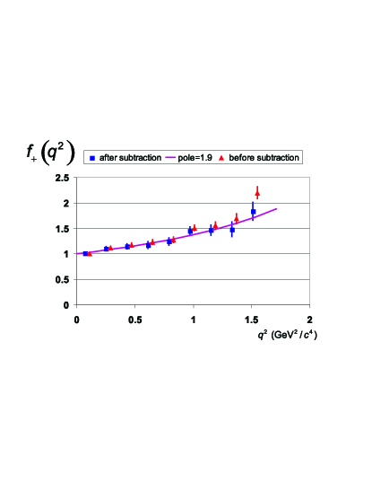
Figure 9: $f_{+}(q^{2}{})$ shapes in $K^{-}\ell+\nu$ obtained by FOCUS focusqsq prior to charm background subtraction triangles and after background subtraction rectangles. The curve is an effective pole fit with $m_{\rm pole}=1.91~{}\rm{GeV}/c^{2}$.

This year, the published results of CLEO III and FOCUS have joined by preliminary results from BaBar, CLEO-c, and Belle. Figure 10 compares their measurement of the $f_{+}(q^{2})$ from $\approx 100K$ $D^{0}\rightarrow K^{-}e^{+}\nu$ to the FOCUS measurements and LQCD predictions milc . BaBar makes this measurement at the $\Upsilon(4S)$ and hence also must neutrino closure techniques similar to FOCUS. Their $q^{2}$ resolution is nearly identical to that of FOCUS and they also have an $\approx 65\%$ negative correlation between $f_{+}(q^{2})$ bins. Apart from the two highest BaBar $q^{2}$ bins, agreement with both FOCUS and the LQCD calculations is good.

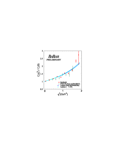
Figure 10: Agreement between the FOCUS and BaBar $f_{+}(q^{2}{})$ shapes in $K^{-}\ell^{+}\nu$. The results are also compared to a recent LQCD calculationmilc

The values are summarized in Table 3 for both $D^{0}\rightarrow K^{-}\ell^{+}\nu$ and $D^{0}\rightarrow\pi^{-}\ell^{+}\nu$. The (preliminary) CLEO-c entry in Table 3 is based on 281 pb^-1 of data taken at the $\psi(3770)$ but does not require a fully reconstructed tagging recoil $\bar{D}^{0}$ unlike most CLEO-c $\psi(3770)$ analyzes. This creates a significant increase in event statistics, but has worse $q^{2}$ resolution than in CLEO-c fully tagged analyzes. The CLEO-c untagged analysis still has an order of magnitude better $q^{2}$ resolution than FOCUS or BaBar.

The $K^{-}\ell^{+}\nu$ measurements do not seem terribly consistent between experiments. My naive weighted average of the $K^{-}\ell^{+}\nu$ values is $\alpha(K^{-}\ell^{+}\nu)=0.35\pm 0.033$ but the CL value that all values are consistent is only 0.9 %. The consistency goes up to 39 % if the preliminary CLEO-c value of $\alpha=0.19$ is excluded. My weighted average of $\alpha(\pi^{-}\ell^{+}\nu)=0.33\pm 0.08$. The consistency CL for all three pion measurements is a respectable 56 %.

Table 3: Modified pole $\alpha$ parameters

	$\alpha(K^{-}\ell^{+}\nu)$	$\alpha(\pi^{-}\ell^{+}\nu)$
CLEO IIIcleoqsq	0.36 $\pm$ 0.10 $\pm$ 0.08	0.37${}^{+0.20}_{-0.31}$ $\pm$ 0.15
FOCUSfocusqsq	0.28 $\pm$ 0.08 $\pm$ 0.07
BaBar	0.43 $\pm$ 0.03 $\pm$ 0.04
CLEO-c	0.19 $\pm$ 0.05 $\pm$ 0.03	0.37 $\pm$ 0.09 $\pm$ 0.03
Belle	0.52 $\pm$ 0.08 $\pm$ 0.06	0.10 $\pm$ 0.21 $\pm$ 0.10
WT AVE	0.35 $\pm$ 0.033	0.33 $\pm$ 0.08

The data on $\alpha(\pi^{-}e^{+}\nu)$ appears to be consistent with that for $\alpha(K^{-}e^{+}\nu)$ as is the case in LQCD calculations. At this point, the pion data are not sufficiently accurate to make a really incisive test of the difference between $\alpha(\pi^{-}e^{+}\nu)$ and $\alpha(K^{-}e^{+}\nu)$.

V Vector $\mathbf{\ell\nu}$ Decays

Although historically vector decays such as $D^{+}\rightarrow\overline{K}^{*0}\ell^{+}\nu$ have been the most accessible semileptonic decays in fixed target experiments owing to their ease of isolating a signal, they are the most complex decays we will discuss. One problem is that a separate form factor is required for each of the three helicity states of the vector meson. Vector $\ell^{+}\nu$ states result in a multihadronic final state. For example $D^{+}\rightarrow\overline{K}^{*0}\ell^{+}\nu$ final states can potentially interfere with $D^{+}\rightarrow K^{-}\pi^{+}\ell^{+}\nu$ processes with the $K^{-}\pi^{+}$ in various angular momentum waves with each wave requiring its own form factor. I will concentrate on form factor measurements of Vector $\ell\nu$ decays.

I believe at present, the $D^{+}\rightarrow K^{-}\pi^{+}\ell^{+}\nu$ and $D_{s}^{+}\rightarrow\phi\ell^{+}\nu$ are the only decays with reasonably well measured form factors. The three decay angles describing the $D^{+}\rightarrow K^{-}\pi^{+}\ell^{+}\nu$ decay are illustrated in Fig. 11. The other kinematic variables are $q^{2}$ and $m_{K\pi}$.

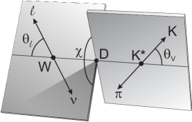
Figure 11: Definition of kinematic variables.

Because the $m_{K\pi}$ distribution in $D^{+}\rightarrow K^{-}\pi^{+}\ell^{+}\nu$ was an excellent fit to the $\overline{K}^{*0}$ Breit-Wigner, it was assumed for many years that any non-resonant component to $D^{+}\rightarrow K^{-}\pi^{+}\ell^{+}\nu$ must be negligible. In 2002, FOCUS observed a strong, forward-backward asymmetry in $\cos\theta_{\textrm{v}}$ for events with $m_{K\pi}$below the $\overline{K}^{*0}$ pole with essentially no asymmetry above the pole as shown in Figure 12.

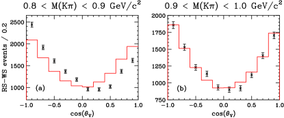
Figure 12: Evidence for s-wave interference in $D^{+}\rightarrow K^{-}\pi^{+}\ell^{+}\nu$.

The simplest explanation for the $\cos\theta_{\textrm{v}}$ asymmetry is an interference between s-wave and p-wave amplitudes creating a linear $\cos\theta_{\textrm{v}}$ term. The phase of the s-wave amplitude must be such that its phase is nearly orthogonal with the Breit-Wigner ($BW$) phase for $m_{K\pi}{}>m(\overline{K}^{*0})$. The (acoplanarity) averaged $|\mathcal{A}|^{2}$ in the zero lepton mass limit (Eq. (12)) is constructed from the Breit-Wigner ($BW$), s-wave amplitude ($Ae^{-i\delta}$), and the helicity basis form factors $H_{+}(q^{2})$, $H_{-}(q^{2})$, $H_{0}(q^{2})$ that describe the $W^{+}$ coupling to each of the $\overline{K}^{*0}$ spin states KS . We also need an additional form factor ($h_{0}(q^{2})$) describing the coupling to the s-wave amplitude.

$$\int{\left|{\rm{A}}\right|^{2}d\chi}=\frac{1}{8}q^{2}\left\{\begin{array}[]{l}\left({(1+\cos\theta_{l})\sin\theta_{V}}\right)^{2}\left|{H_{+}(q^{2})}\right|^{2}\left|{BW}\right|^{2}\\ +\left({(1-\cos\theta_{l})\sin\theta_{V}}\right)^{2}\left|{H_{-}(q^{2})}\right|^{2}\left|{BW}\right|^{2}\\ +\left({2\sin\theta_{l}\cos\theta_{V}}\right)^{2}\left|{H_{0}(q^{2})}\right|^{2}\left|{BW}\right|^{2}\\ +8\left({\sin^{2}\theta_{l}\cos\theta_{V}}\right)H_{0}(q^{2})h_{o}(q^{2}){\mathop{\rm Re}\nolimits}\left\{{Ae^{-i\delta}BW}\right\}\\ +O(A^{2}).\\ \end{array}\right\}$$ (12)

The $H_{+}(q^{2})$, $H_{-}(q^{2})$, and $H_{0}(q^{2})$ form factors are linear combinations of two axial and one vector form factor as indicated in Eq. (V).

$$H_{\pm}(q^{2}) = (M_{D}+m_{K\pi})A_{1}(q^{2})\mp 2{M_{D}K\over M_{D}+m_{K\pi}}V(q^{2})\,,$$

$$H_{0}(q^{2}) = {1\over 2m_{K\pi}\sqrt{q^{2}}}\left[(M^{2}_{D}-m^{2}_{K\pi}-q^{2})(M_{D}+m_{K\pi})A_{1}(q^{2})-4{M^{2}_{D}K^{2}\over M_{D}+m_{K\pi}}A_{2}(q^{2})\right].$$

Eq. (LABEL:helform) shows that as $q^{2}{}\rightarrow 0$, both $H_{+}(q^{2})$ and $H_{-}(q^{2})$ approach a constant. Since the helicity intensity contributions are proportional to $q^{2}{}H^{2}_{\pm}(q^{2}{})$ ( Eq. (12)) the $H_{\pm}$ intensity contributions vanish in this limit. Figure 13 explains why this is true. As $q^{2}{}\rightarrow 0$, the $e^{+}$ and $\nu$ become collinear with the virtual $W^{+}$. For $H_{+}(q^{2})$ and $H_{-}(q^{2})$, the virtual $W^{+}$ must be in either the $|1,\pm 1\rangle$ state which means that the $e^{+}$ and $\nu$ must both appear as either righthanded or lefthanded thus violating the charged current helicity rules. Hence $q^{2}{}H_{\pm}(q^{2}{})$ vanishes at low $q^{2}$. For $H_{0}(q^{2})$, the $W^{+}$ is in $|1,0\rangle$ state thus allowing the $e^{+}$ and $\nu$ to be in their (opposite) natural helicity state. Hence at low $q^{2}$, $H_{0}(q^{2}){}\rightarrow 1/\sqrt{q^{2}{}}$ which allows for $D^{+}\rightarrow\overline{K}^{*0}\mu^{+}\nu$ decays as $q^{2}{}\rightarrow 0$. Presumably $h_{0}(q^{2}){}\rightarrow 1/\sqrt{q^{2}{}}$ as well since it also describes a process with $W^{+}$ is in $|1,0\rangle$ state

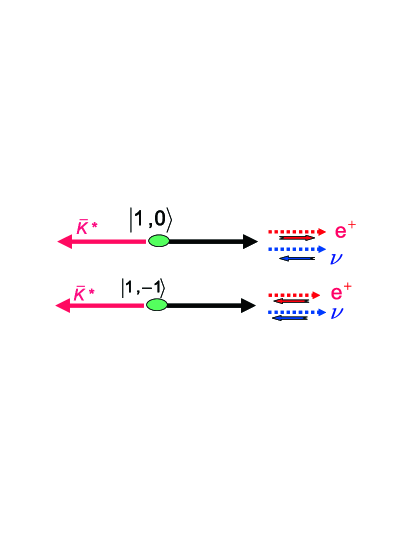
Figure 13: The electron helicity state in the low $q^{2}$ limit. When the virtual $W^{+}$ is in the zero helicity state, the $e^{+}$ and $\nu$ have the opposite helicity and can be in their charged-current helicity states. When the virtual $W^{+}$ is in the $\langle 1,\pm 1\rangle$ state the $e^{+}$ and $\nu$ must be in the same helicity states and violate the weak helicity rules.

Vector $\ell^{+}\nu$ processes have been traditionally analyzed using a spectroscopic pole dominance model for $V(q^{2}{})$, $A_{1}(q^{2}{})$ and $A_{2}(q^{2})$. The vector pole is at the mass of the $D_{s}^{*}$ ; while both axial poles are set to 2.5 GeV.

Under these assumptions the shape of the $D^{+}\rightarrow\overline{K}^{*0}\mu^{+}\nu$ intensity (apart from the s-wave effect) is fully determined from the ratio of the axial and vector form factors at $q^{2}$ = 0. Traditionally the variables are $r_{v}=V(0)/A_{1}(0)$ and $r_{2}=V(0)/A_{1}(0)$. A long series of measurements has been made for $D^{+}\rightarrow\overline{K}^{*0}\ell^{+}\nu$ and $D_{s}^{+}\rightarrow\phi\;\ell^{+}\nu$ over the years under the assumption with spectroscopic pole dominance oldformfactor . A wide range of theoretical techniques have been employed to predict the form factor ratios more or less successfully quark lqcd ball . Figures 14 summarize these measurements. My weighted average is $r_{v}=1.618\pm 0.055$ and $r_{2}=0.830\pm 0.054$ with a confidence level of 6.7% that all $r_{v}$ values are consistent and 42% that all $r_{2}$ values are consistent. Only the latest measurement by FOCUS includes the s-wave contribution– including it with the ad-hoc assumption that the $h_{0}(q^{2})$ form factor for the $K\pi$ s-wave contribution is the same as the $H_{0}(q^{2})$ form factor for the zero helicity $\overline{K}^{*0}$contribution.

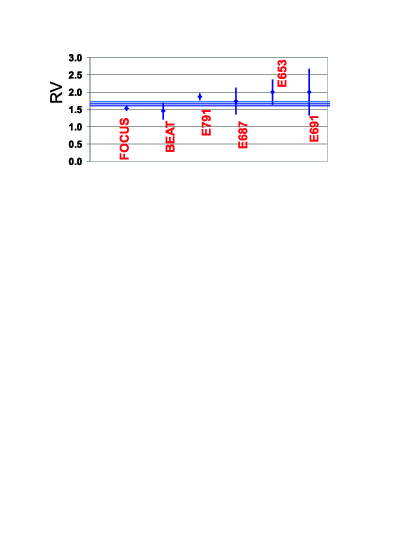
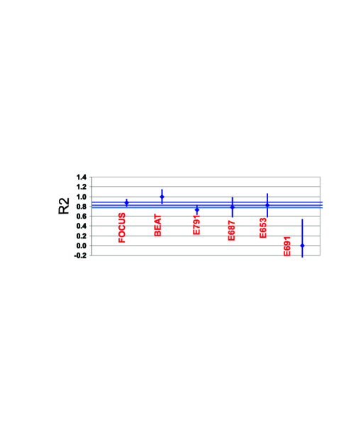
Figure 14: The $r_{v}$and $r_{2}$form factor ratios for $D^{+}\rightarrow\overline{K}^{*0}\ell^{+}\nu$ measured by six experiments. The blue lines are the weighted average of all six measurements.

The experimental situation with $D_{s}^{+}\rightarrow\phi\;\ell^{+}\nu$ shown in Fig. 15 is somewhat less clear phigoof . By SU(3) symmetry and explicit calculation, the $r_{v}$ and $r_{2}$ form factor ratios for $D^{+}\rightarrow\overline{K}^{*0}\ell^{+}\nu$ and $D_{s}^{+}\rightarrow\phi\;\ell^{+}\nu$ decays are expected to lie within $\approx 10\%$ of each other russian . This is true for $r_{v}$, but previous to the very recent measurement by the FOCUS focusphi , $r_{2}$ for $D_{s}^{+}\rightarrow\phi\;\ell^{+}\nu$ was roughly a factor of two larger than that for $D^{+}\rightarrow\overline{K}^{*0}\ell^{+}\nu$ although there is a 27% confidence level that all published $r_{2}$ values for $D_{s}^{+}\rightarrow\phi\;\ell^{+}\nu$ are consistent.

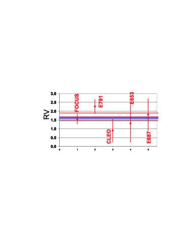
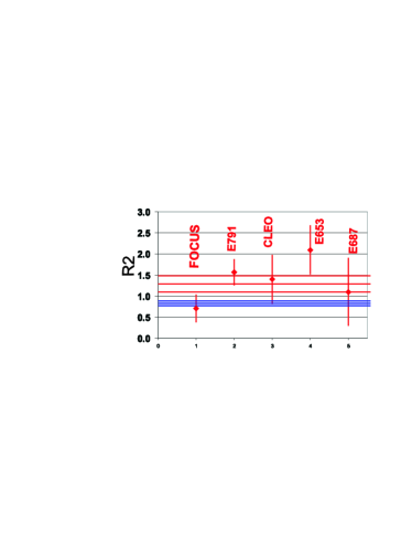
Figure 15: The $r_{v}$and $r_{2}$form factor ratios for $D_{s}^{+}\rightarrow\phi\;\ell^{+}\nu$ measured by five experiments. The blue lines are the weighted average of the $D^{+}\rightarrow\overline{K}^{*0}\ell^{+}\nu$ form factors shown in Fig. 14. It was expected that the $D_{s}^{+}\rightarrow\phi\;\ell^{+}\nu$ form factors should be consistent with the $D^{+}\rightarrow\overline{K}^{*0}\ell^{+}\nu$ form factors.

Given the failure of the spectroscopic pole model in pseudoscalar $\ell^{+}\nu$ decays, and the fact that the $q^{2}{}_{\rm max}$ for $D^{+}\rightarrow\overline{K}^{*0}\ell^{+}\nu$ is even further from the $D_{s}^{+*}$ pole than the case for $K^{-}\ell+\nu$ it seems unlikely that spectroscopic pole dominance is a good model for axial and vector form factors relevant to vector $\ell^{+}\nu$ decay. Although most groups reporting $r_{v}$ and $r_{2}$ values show that their fits roughly reproduce the various $\cos\theta_{\textrm{v}}$, $\cos\theta_{\ell}$, $q^{2}$, and $\chi$ projections observed in their data, there have been no quantitative tests to my knowledge on the validity of the the spectroscopic pole assumptions in vector $\ell^{+}\nu$ charm decay. Fajfer and Kamenik FK have proposed an effective pole descriptions of the vector and two axial form factors used in Eq. (12). For example their $V(q^{2})$ parameterization is identical to the $f_{+}(q^{2}{})$ given in Eq. (6). But I know of no attempts to fit for either the effective pole parameters of Fajfer and Kamenik or simple effective poles such as those displayed in Fig. 7 for $K^{-}\ell^{+}\nu$. The problem is that the spectroscopic pole constraint is such a powerful constraint that releasing it would severely inflate errors on $r_{v}$ and $r_{2}$.

As a first attempt to study $D^{+}\rightarrow\overline{K}^{*0}\ell^{+}\nu$ free from the constraining assumption of spectroscopic pole dominance, FOCUS focus-helicity developed a non-parametric method for studying the helicity basis form factors. As shown in Eq. (12), after integration by the acoplanarity $\chi$ to kill interference between different helicity states, the decay intensity greatly simplifies into a sum of just four terms proportional to: $H^{2}_{0}(q^{2})$, $H^{2}_{+}(q^{2})$, $H_{-}(q^{2})$, and $h_{0}(q^{2})\,H_{0}(q^{2})$. Each term is associated with a unique angular distribution which can be used to project out each individual term. The projection can be done by making 4 weighted histograms using projective weights based on the $\cos\theta_{\textrm{v}}$ and $\cos\theta_{\ell}$ for each event.

Figure 16 shows the four weighted histograms from a preliminary analysis of 281 pb^-1 of $\psi(3770)$ CLEO data. The CLEO data are far superior for this analysis because of its nearly order of magnitude better $q^{2}$ resolution than the resolution in a fixed target experiment such as FOCUS.

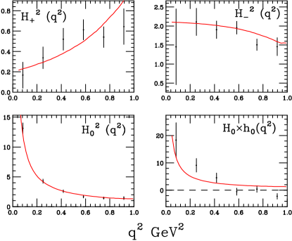
Figure 16: The four helicity form factor products obtained in a preliminary analysis using 281 pb^-1 data set from CLEO. The curves represent the model of Reference formfactor .

Figure 16 shows the expected behavior that $H^{2}_{\pm}(q^{2}{})\rightarrow{\rm constant}$ as $q^{2}{}\rightarrow 0$ while $H^{2}_{0}(q^{2})$ and $h_{0}(q^{2})\,H_{0}(q^{2})$ approaches $1/q^{2}{}$. The curves give the helicity form factors according to Eq. (12), using spectroscopic pole dominance and the $r_{v}$, $r_{2}$, and s-wave parameters measured by FOCUS. Apart from the $h_{0}(q^{2})\,H_{0}(q^{2})$ form factor product the spectroscopic pole dominance model is a fairly good match to the CLEO non-parametric analysis. This suggests that the ad-hoc assumption that $h_{0}(q^{2})$=$H_{0}(q^{2})$ is questionable but it will probably take more data to gain insight into the nature of the discrepancy.

Figure 17 gives a different insight into the helicity basis form factors by plotting the intensity contributions of each of the form factor products. This is the form factor product multiplied by $q^{2}$. Since $q^{2}$$H^{2}_{0}(q^{2})$ is nearly constant, we normalized form factors such that $q^{2}{}H^{2}_{0}(q^{2}){}=1$ at $q^{2}$ = 0. As one can see from Eq. (12), both $q^{2}$$H^{2}_{+}(q^{2})$ and $q^{2}$$H^{2}_{-}(q^{2})$ rise from zero with increasing $q^{2}$ until they both equal $q^{2}$$H^{2}_{0}(q^{2})$ at $q^{2}$_max. As $q^{2}$ is increased from 0 the $D^{+}\rightarrow\overline{K}^{*0}\ell^{+}\nu$ $\theta_{V}$ distribution evolves from $\cos\theta_{\textrm{v}}^{2}$ (100 % longitudinally polarized) to a flat distribution (unpolarized).

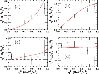
Figure 17: Non-parametric form factor products obtained for the data sample (multiplied by $q^{2}$) The reconstructed form factor products are shown as the points with error bars, where the error bars represent the statistical uncertainties. The solid curves in the histograms represent a form factor model described in Ref. formfactor . The histogram plots are: (a) $q^{2}{}H_{+}^{2}(q^{2})$, (b) $q^{2}{}H_{-}^{2}(q^{2})$, (c) $q^{2}{}H_{0}^{2}(q^{2})$, and (d) $q^{2}{}h_{0}(q^{2})H_{0}(q^{2})$. The form factors are normalized such that $q^{2}{}h_{0}(q^{2})H_{0}(q^{2})\rightarrow 1$ as $q^{2}{}\rightarrow 0$.

What can we learn about the pole masses? Unfortunately Fig. 18 shows that the present data are insufficient to learn anything useful about the pole masses. On the left of Figure 18 the helicity form factors are compared to a model generated with the FOCUS form factor ratios and the standard pole masses of 2.1 GeV for the vector pole and 2.5 GeV for the two axial poles. On the right side of Fig. 18 the form factors are compared to a model where the pole masses are set to infinity. Both models fit the data equally well.

What can we learn about the phase of the s-wave contribution? Recall in Figure 12 the $\cos\theta_{\textrm{v}}$ asymmetry created by the interference between the s-wave and $D^{+}\rightarrow\overline{K}^{*0}\ell^{+}\nu$ only appeared below the $\overline{K}^{*0}$pole in FOCUS data and meaning that the s-wave phase was orthogonal with the $m_{K\pi}>m(\overline{K}^{*0})$ half of the Breit-Wigner amplitude. As Figure 19 shows, the same thing happens in CLEO data : the effective $h_{0}(q^{2})\,H_{0}(q^{2})$ disappears above the $\overline{K}^{*0}$pole and is very strong below the pole. The amplitude $A$ of the s-wave piece is arbitrary since using interference we can only observe the product $A~{}h_{0}(q^{2}{})$. This means any change in $A$ scale can be compensated by a change of scale in $h_{0}(q^{2}{})$. The fact that the $h_{0}(q^{2})\,H_{0}(q^{2})$ data was a tolerable match (at least in the low $q^{2}$ region) to the FOCUS curve in Figure 16 does imply, however, that the s-wave amplitude observed in CLEO is consistent with that of FOCUS. A more formal fit of the s-wave parameters is in progress.

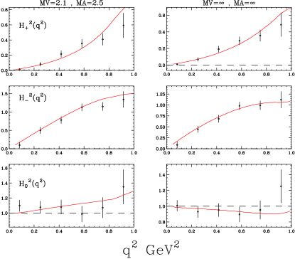
Figure 18: Non-parametric form factor products obtained for data (multiplied by $q^{2}$) The solid curves are based on the $s$-wave model and measurements described in Reference formfactor The reconstructed form factor products are the points with error bars. The three plots on the right are the usual model with the spectroscopic pole masses; while the three plots on the right are run with all pole masses with the axial and vector pole masses taken to infinity

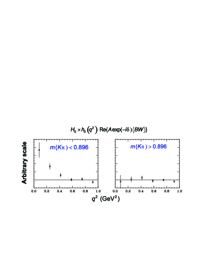
Figure 19: The s-wave interference term for events below the $\overline{K}^{*0}$ pole (left) and above the pole (right). The interference term depends on the s-wave phase relative to the phase average phase of each half of the Breit-Wigner. All of the $\cos\theta_{\textrm{v}}$ interference observed by FOCUS was also below the $\overline{K}^{*0}$pole as shown in Fig. 12

Finally, is there evidence for higher $K^{-}\pi^{+}$ angular momentum amplitudes in $D^{+}\rightarrow K^{-}\pi^{+}\ell^{+}\nu$? We searched for possible additional interference terms such as a $d$-wave contribution:

$$4\,\sin^{2}\theta_{\ell}~{}\cos\theta_{\textrm{v}}~{}(3\,\cos^{2}\theta_{\textrm{v}}-1)\,H_{0}(q^{2})\,h^{(d)}_{0}(q^{2})\,{\mathop{\mathrm{Re}}\nolimits}\{\mathrm{A}_{d}e^{-i\delta_{d}}\textrm{BW}\}$$

or an $f$-wave contribution:

$$4\,\sin^{2}\theta_{\ell}~{}\cos\theta_{\textrm{v}}~{}(5\,\cos^{3}\theta_{\textrm{v}}-3\cos\theta)\,H_{0}(q^{2})\,h^{(f)}_{0}(q^{2})\,{\mathop{\mathrm{Re}}\nolimits}\{A_{f}e^{-i\delta_{f}}\textrm{BW}\}.$$

As shown in Figure 20 there is no evidence for such additional contributions:

Figure 20: Search for (a) $d$-wave and (b) $f$-wave interference effects as described in the text.

VI Summary

A great deal of progress has been made in charm semileptonic decay in the last few years. A new set of precision semileptonic branching ratios have been made available from CLEO. These include both exclusive mesonic branching fractions as well as inclusive semileptonic branching fractions for the $D^{0}$ and $D^{+}$. This data suggests that the known exclusive decays comes close to saturating the measured inclusive branching fraction, and that the inclusive semileptonic widths for the $D^{+}$ and $D^{0}$ are equal as expected.

The first precision measurements of charm fully leptonic decay have been made by CLEO ($D^{+}\rightarrow\mu^{+}\nu$) and BaBar ($D_{s}^{+}\rightarrow\mu^{+}\nu$). Both experiments produce $\approx 8\%$ measurements of the meson decay constants ($f_{D}$) that are consistent with LQCD calculations and with comparable uncertainty to the calculations.

Several new precision, non-parametric measurements have been made of the $f_{+}(q^{2}{})$ form factor in $D^{0}\rightarrow K^{-}\ell^{+}\nu$. At present the situation is a bit murky. The earlier measurements, tend to agree with each other as well as the LQCD calculations on the form factor shape. One of the new preliminary measurement has a significantly different shape parameter $\alpha$.

Finally progress in understanding vector $\ell^{+}\nu$ decays was reviewed. These have historically been analyzed under the assumption of spectroscopic pole dominance. Experiments have obtained consistent results under this assumption, but as of yet there have been no incisive tests of spectroscopic pole dominance. We concluded by describing a first, preliminary non-parametric look at the $D^{+}\rightarrow K^{-}\pi^{+}\ell^{+}\nu$ form factors. Although the results were very consistent with the traditional pole dominance fits, the data was not precise enough to incisively measure $q^{2}$ dependence of the axial and vector form factors and thus test spectroscopic dominance. This preliminary analysis confirms the existence of an $s$-wave effect first observed by FOCUS swave , and was unable to obtain evidence for $d$ and $f$-waves.

References

- (1) CLEO Collaboration, Q. He et al., Phys. Rev. Lett. 95, 121801 (2005).
- (2) CLEO Collaboration, G. S. Huang et al., Phys. Rev. Lett. 95, 181801 (2005); CLEO Collaboration, G. S. Huang et al., Phys. Rev. Lett. 95, 181802 (2005).
- (3) CLEO Collaboration, M. Artuso et al., Phys. Rev. Lett. 95, 251801 (2005).
- (4) C. Aubin et al., Phys. Rev. Lett. 95, 122002 (2005).
- (5) CLEO Collab., Phys. Lett B317, 647,(1993); E691 Collab., J.C. Anjos, Phys. Rev. Lett. 62,1587 (1989); CLEO Collab., Phys. Rev. D44, 3394 (1991); Mark III Collab., Phys. Rev. Lett. 66, 1011 (1991); E687 Collab., P.L. Frabetti et al., Phys. Lett. B364, 127,(1995); FOCUS Collaboration, J.M. Link et al., Phys. Lett. B607 233-242 (2005); CLEO Collaboration, G. S. Huang et al., Phys. Rev. Lett. 94, 011802 (2005).
- (6) D.Becirevic and A. Kaidalov, Phys. Lett. B478, 417-423(2000)
- (7) Richard J. Hill, Phys.Rev. D73 (2006) 014012
- (8) FOCUS Collaboration, J.M. Link et al., Phys. Lett. B607 233-242 (2005).
- (9) CLEO Collaboration, G. S. Huang et al., Phys. Rev. Lett. 94, 011802 (2005).
- (10) J.G. Korner and G.A. Schuler, Z. Phys. C 46, 93 (1990).
- (11) FOCUS Collaboration, J.M. Link et al., Phys. Lett. B 544, 89 (2002); BEATRICE Collab., M. Adamovich et al., Eur. Phys. J. C 6 (1999) 35; E791 Collab., E. M. Aitala et al., Phys. Rev. Lett. 80 (1998) 1393; E791 Collab., E. M. Aitala et al., Phys. Lett. B 440 (1998) 435; Phys. Lett. B 307 (1993) 262; E653 Collab., K. Kodama et al., Phys. Lett. B 274 (1992) 246; E691 Collab., J. C. Anjos et al., Phys. Rev. Lett. 65 (1990) 2630.
- (12) M. Bauer, B. Stech, and M. Wirbel, Z. Phys. C 29, 637 (1985); M. Bauer and M. Wirbel, Z. Phys. C 42, 671 (1989); J.G. Korner and G.A. Schuler, Z. Phys. C 46, 93 (1990); F.J. Gilman and R.L. Singleton, Phys. Rev. D 41, 142 (1990); D. Scorna and N. Isgur, Phys. Rev. D 62, 2783 (1995); B. Stech, Z. Phys. C 75, 245 (1997); D. Melikhov and B. Stech, Phys. Rev. D 62, 014006 (2000).
- (13) C.W. Bernard, A.X. El-Khadra, and A. Soni, Phys. Rev. D 45, 869 (1992); V. Lubicz, G. Martinelli, M.S. McCarthy, and C.T. Sachrajda, Phys. Lett. B 274, 415 (1992); A. Abada et al., Nucl. Phys. B 416, 675 (1994); UKQCD Collaboration, K.C. Bowler et al., Phys. Rev. D 51, 4905 (1995); T. Bhattacharya and R. Gupta, Nucl. Phys. B (Proc. Suppl.) 47, 481 (1996); APE Collaboration, C.R. Alton et al., Phys. Lett. B 345, 513 (1995); S. Gusken, G. Siegert, and K. Schilling, Prog. Theor. Phys. Suppl. 122, 129 (1996); SPQcdR Collaboration, A. Abada et al., Nucl. Phys. Proc. Supp. 119, 625 (2003).
- (14) P. Ball, V.M. Braun, H.G. Dosch, and M. Neubert, Phys. Lett. B 259, 481 (1991); P. Ball, V.M. Braun, and H.G. Dosch, Phys. Rev. D 44, 3567 (1991).
- (15) S.S.Gershtein, M.Yu.Khlopov , Pis’ma v ZhETF V.23, 374-377 (1976). [English translation: JETP Lett. V.23, 338 (1976)]; M.Yu.Khlopov, Yadernaya Fizika V. 28, 1134-1137 (1978) [English translation: Sov.J.Nucl.Phys. V. 28, no. 4, 583(1978)].
- (16) FOCUS Collaboration, J.M. Link et al., Phys. Lett. B 586(2004)183
- (17) E791 Collab. E.M. Aitala et al., Phys. Lett. B 450 (1999) 294; CLEO Collab. P. Avery et al., Phys. Lett. B 337 (1994) 405; E687 Collab. P. L. Frabetti et al., Phys. Lett. B 328 (1994) 187; E653 Collab. K. Kodama et al., Phys. Lett. B 309 (1993) 483.
- (18) S. Fajfer and J. Kamenik, Phys. Rev. D 72, 034029 (2005).
- (19) FOCUS Collaboration, J.M. Link et al., Phys. Lett. B 633, 183 (2006).
- (20) FOCUS Collaboration, J.M. Link et al., Phys. Lett. B 544, 89 (2002).
- (21) FOCUS Collaboration, J.M. Link et al., Phys. Lett. B 535, 43 (2002).