NORTHWESTERN UNIVERSITY
Precision Measurements of the Timelike Electromagnetic Form Factors of the Pion, Kaon, and Proton
A DISSERTATION
SUBMITTED TO THE GRADUATE SCHOOL
IN PARTIAL FULFILMENT OF THE REQUIREMENTS
for the degree
DOCTOR OF PHILOSOPHY
Field of Physics and Astronomy
By
Peter Karl Zweber
EVANSTON, ILLINOIS
June 2006

 ABSTRACT

Precision Measurements of the Timelike Electromagnetic Form Factors of the Pion, Kaon, and Proton

Peter Karl Zweber

Using 20.7 pb^-1 of $e^{+}e^{-}$ annihilation data taken at $\sqrt{s}=3.671$ GeV with the CLEO–c detector, precision measurements of the electromagnetic form factors of the charged pion, charged kaon, and proton have been made for timelike momentum transfer of $|Q^{2}|=13.48$ GeV² by the reaction $e^{+}e^{-}\to h^{+}h^{-}$. The measurements are the first ever with identified pions and kaons of $|Q^{2}|>4$ GeV², with the results $|F_{\pi}(13.48\;\mathrm{GeV}^{2})|=0.075\pm 0.008(\mathrm{stat})\pm 0.005(\mathrm{syst})$ and $|F_{K}(13.48\;\mathrm{GeV}^{2})|=0.063\pm 0.004(\mathrm{stat})\pm 0.001(\mathrm{syst})$. The result for the proton, assuming $|G^{P}_{E}(Q^{2})|=|G^{P}_{M}(Q^{2})|$, is $|G^{P}_{M}(13.48\;\mathrm{GeV}^{2})|=0.0139^{+0.0024}_{-0.0018}(\mathrm{stat})\pm 0.0006(\mathrm{syst})$, which is in agreement with earlier results.

To my parents, brothers, and Adie, for all of their support and patience.

Chapter 1 Introduction

This dissertation is devoted to the study of the structure of the three lightest strongly interacting hadrons, the two lightest mesons, the pion and the kaon, and the lightest baryon, the proton, by measuring their electromagnetic form factors. In order to put this study in perspective, it is useful to briefly review particle physics.

The study of particle physics is the study of fundamental particles and the interactions between them. The modern framework which incorporates the fundamental particles and interactions is called the Standard Model. There are four fundamental interactions, and they are, in decreasing order of strength, the strong (often called nuclear or hadronic), electromagnetic, weak, and gravitational. With respect to the strong interaction, the relative strength of the electromagnetic, weak, and gravitational interactions are $\sim 1/137$, $10^{-5}$, and $10^{-39}$ [1], respectively. The gravitational interaction is not yet well understood and is not included in the Standard Model.

Particles are called fundamental when they are structureless and pointlike. While being structureless, fundamental particles have an intrinsic property called spin. The spin of particles, fundamental or composite, have either integer or half-integer values. Particles with integer values of spin are governed by Bose-Einstein statistics and are hence called bosons, and particles with half-integer values are governed by Fermi-Dirac statistics and are called fermions.

The strong, electromagnetic, and weak interactions are all mediated by spin-1 vector bosons. The strong interaction is mediated by gluons (denoted by $g$), electromagnetism by photons ($\gamma$), and the weak by $W$ and $Z$ bosons. Table 1.1 lists the various properties of the mediators.

Table 1.1: Fundamental interaction mediators in the Standard Model. The numerical values are taken from Ref. [2]. The electric charge $|e|$ is the charge of an electron, $|e|$ = 1.602$\times 10^{-19}$ Coulombs.

Force	Mediator	Electric	Mass (GeV)
		Charge
Strong	$g$	0	0
Electromagnetic	$\gamma$	0	0
Weak	$W^{\pm}$	$\pm$1$|e|$	80.425(38)
	$Z^{0}$	0	91.1876(21)

The fundamental particles which comprise all of the known matter in the universe are spin-1/2 fermions. The particles which can interact strongly are called quarks and the ones which cannot are called leptons. For every charged lepton, there is a corresponding weakly interacting partner, the neutrino. For example, the lightest charged lepton is the electron ($e$), and its corresponding neutrino partner is called the electron neutrino ($\nu_{e}$). The charged-and-neutrino lepton combination forms a family or generation. Two other families of leptons exist. They are the muon ($\mu$) and tau ($\tau$) and the corresponding muon neutrino ($\nu_{\mu}$) and tau neutrino ($\nu_{\tau}$). The $\mu$ and $\tau$ have the same general properties as the electron except with larger masses. Just as the leptons can be formed into generations, the quarks are also grouped into generations. The first generation of quarks consists of the up ($u$) and down ($d$) quarks, the second consists of the strange ($s$) and charm ($c$) quarks, and the third consists of the bottom ($b$) and top ($t$) quarks. The type of quark is also called the flavor of the quark. Table 1.2 lists the properties of the fundamental fermions. Each fundamental fermion has a corresponding antiparticle, which has the opposite charge.

Table 1.2: Fundamental particles in the Standard Model. The numerical values are taken from Ref. [2]. The electric charge $|e|$ is the charge of an electron, $|e|$ = 1.602$\times 10^{-19}$ Coulombs. The masses of the quarks are the so-called ’current quark masses’. The upper limits on the neutrino masses are at 90$\%$ confidence level.

	Leptons			Quarks
Generation	Name	Electric	Mass	Name	Electric	Mass
or Family		Charge			Charge
I	$e^{-}$	$-1|e|$	511 keV	$u$	$+\frac{2}{3}|e|$	1.5$-$4 MeV
	$\nu_{e}$	0	$<$ 3 eV	$d$	$-\frac{1}{3}|e|$	4$-$8 MeV
II	$\mu^{-}$	$-1|e|$	106 MeV	$c$	$+\frac{2}{3}|e|$	1.15$-$1.35 GeV
	$\nu_{\mu}$	0	$<$ 0.19 keV	$s$	$-\frac{1}{3}|e|$	80$-$130 MeV
III	$\tau^{-}$	$-1|e|$	1.78 GeV	$t$	$+\frac{2}{3}|e|$	174 GeV
	$\nu_{\tau}$	0	$<$ 18.2 eV	$b$	$-\frac{1}{3}|e|$	4.1$-$4.4 GeV

As mentioned above, not all of the fundamental fermions participate in all three interactions. The quarks interact through all three interactions, the charged leptons only through the electromagnetic and weak, and neutrinos only via the weak. The vector bosons mediating the interaction couple to the ’charges’ of the particles. The most familiar type of charge is electric charge. The propagator of the electromagnetic interaction, the photon, couples to the electric charge of the particle. The propagators of the weak interactions, the $W$ and $Z$, couple to the fermions through the so-called the ’weak’ charge. The strong force couples through the so-called the ’color’ charge, first described by Greenberg [3] in 1964. While there is only one type of electric charge (positive ($+$) and negative ($-$)), color has three charges denoted by red, blue, and green ($r,b,g$, and $\overline{r},\overline{b},\overline{g}$). The strong interaction is described by the SU(3) symmetry group called color SU(3). One possible representation of this symmetry group is

$$r\overline{g},~{}~{}r\overline{b},~{}~{}g\overline{b},~{}~{}g\overline{r},~{}~{}b\overline{r},~{}~{}b\overline{g},~{}~{}\sqrt{\frac{1}{2}}(r\overline{r}-g\overline{g}),~{}~{}\sqrt{\frac{1}{6}}(r\overline{r}+g\overline{g}-b\overline{b}),$$ (1.1)

where $r$, $\overline{r}$, $g$, $\overline{g}$, $b$, and $\overline{b}$, denote the red, antired, green, antigreen, blue, and antiblue color charges, respectively. Each color combination listed in Eqn. 1.1 is ascribed to a gluon.

Another facet of the strong interaction is that free quarks do not exist in nature. Quarks bind together into particles called hadrons. Hadrons have only been observed in two configurations; quark-antiquark pairs ($q\overline{q}$) and quark triplets ($qqq$). The former are called mesons and have integer spin values, while the latter are called baryons and have half-integer spins. Hadrons are color neutral. For a given meson, the quark possesses one type of color charge while the antiquark possesses its anticolor. The convention for baryons to be color neutral is for each quark to have a different color. The mechanism for the absence of free quarks is called confinement, whose origin is related to the fact that gluons themselves carry color. Since gluons carry color, they can bind to each other. This self-coupling phenomena is not present in electromagnetism because the photons are electrically neutral.

The quantum theory describing the strong interaction is called Quantum Chromodynamics (QCD). It is described by the QCD Lagrangian [2]

$${\cal L}=-\frac{1}{4}F^{a}_{\mu\nu}F^{a\mu\nu}+\sum_{q}\overline{\psi_{q}}(i{\not\!D}-m_{q})\psi_{q},$$ (1.2)

where $F^{a}_{\mu\nu}$ is the strength of the gluon field, $\psi_{q}$ is the quark wave function, $\not\!D$ is the covariant derivative, $m_{q}$ is the quark mass, and $a$ is an index for the three color charges. The strength of the gluon field is given by

$$F^{a}_{\mu\nu}=\partial_{\mu}A^{a}_{\nu}-\partial_{\nu}A^{a}_{\mu}+gf^{abc}A^{b}_{\mu}A^{c}_{\nu},$$ (1.3)

where $A^{i}_{\nu}$ $(i=a,b,c)$ are the gauge potentials of the gluon fields, $g$ is coupling constant for the gluon, and $f^{abc}$ are the structure constants of the gauge group. The covariant derivative is given by

$$\not\!D_{\mu}=\partial_{\mu}-ig\sum_{a}A^{a}_{\mu}t^{a},$$ (1.4)

where $t^{i}$ are the gauge representation matrices. The coupling constant $g$ is normally rewritten in terms of the strong coupling constant $\alpha_{s}$ = $g^{2}/4\pi$.

The strong interaction can be characterized by an empirical potential. A commonly used potential is the so-called Cornell potential [4],

$$V_{strong}=\frac{\kappa}{r}+br,$$ (1.5)

where $r$ is the interquark distance and $\kappa$ and $b$ are coefficients with units of
(energy)$\cdot$(length) and (energy)/(length), respectively. The $1/r$ part describes the standard Coulombic potential of the electromagnetic interaction. The part proportional to $r$ describes the confinement aspect of the potential; the larger the distance between the quarks, the larger the force binding them together. Potentials are only a simple approximation to the theory of strong interactions which is described in terms of quantum field theory.

In 1974, Wilson [5] showed how to quantize a gauge field theory on a discrete lattice in Euclidean space-time preserving exact gauge invariance. He applied this calculational technique to the strong coupling regime of QCD. In these Lattice Gauge calculations (Lattice QCD), space-time is replaced by a four dimensional hypercubic lattice of size $L^{3}T$. The sites are separated by the lattice spacing $a$. The quarks and gluons fields are defined at discrete points. Physical problems are solved numerically by Monte Carlo simulations requiring only the quarks masses as input parameters.

An important simplification used with quantum field theories is the perturbative expansion. Experimentally, only the initial and final states of an interaction are observed while the internal action is not. Theoretical models and predictions are made to describe the nature of the unobserved interaction. The simplest interaction is when a single mediating boson interacts between the initial and final states. At each point that the mediator couples to a particle, a coupling constant is added the overall process. There are also processes which include more than one internal interaction. The more the internal interactions, the larger the number of coupling constants that are included in the final process. If the coupling constant is small, the more complicated internal processes (higher order processes) have a lower significance in the overall process. For example, the quantum theory describing the electromagnetic interaction, Quantum Electrodynamics (QED), has a coupling constant which is given by the fine-structure constant $\alpha$ = $e^{2}/(4\pi\epsilon_{0}\hbar c)$ = $1/137$, where $e$ is the charge of an electron, $\epsilon_{0}$ is the permittivity of free space, $\hbar$ is the Planck constant,and c is the speed of light. An example QED process is dimuon production from $e^{+}e^{-}$ annihilations, i.e.,

$$e^{+}e^{-}\rightarrow\mu^{+}\mu^{-}.$$ (1.6)

Feymann diagrams for this process are shown in Figure 1.1. The lowest order term is the $e^{+}e^{-}$ annihilating to a virtual photon followed by that photon producing a $\mu^{+}\mu^{-}$ pair. Figure 1.1 also shows some example higher order processes. At each point where a photon couples to a fermion line, one order of $\sqrt{\alpha}$ is added to the process. Each of the higher order processes have an extra $\alpha$ term. Their contribution to the overall process is at the percent level. The higher order electromagnetic processes can therefore be neglected because the electromagnetic coupling constant $\alpha$ is small.

Figure 1.1: Feymann diagrams for $e^{+}e^{-}\rightarrow\mu^{+}\mu^{-}$. The top figure is the lowest order process. The bottom figures are higher order corrections.

A major difficulty with QCD is the size of strong coupling constant. Gross and Wilczek [6] and Politzer [7] showed that the strong coupling constant is energy dependent ($\alpha_{s}\rightarrow\alpha_{s}(\mu)$, where $\mu$ is the energy scale), and it decreases with increasing energy. The one loop form of the strong coupling constant is

$$\alpha_{s}(\mu)=\frac{4\pi}{\beta~{}\mathrm{ln}(\mu^{2}/\Lambda^{2})},$$ (1.7)

where $\beta=11-\frac{2}{3}n_{f}$, $n_{f}$ is the number of flavors, and $\Lambda=0.2-0.3$ GeV is the QCD scale parameter. Figure 1.2 shows the variation of $\alpha_{s}(\mu)$ as a function of energy; it decreases from $\sim$0.25 at 3 GeV to $\sim$0.11 at 100 GeV. As $\mu\rightarrow\infty$, $\alpha_{s}(\mu)\rightarrow 0$. This behavior is called asymptotic freedom, and therefore QCD is said to be asymptotically free. For small $\alpha_{s}(\mu)$, perturbative calculations can be made, and the formalism is called Perturbative Quantum Chromodynamics (PQCD). PQCD has been used to describe the electromagnetic form factors of hadrons, as described later.

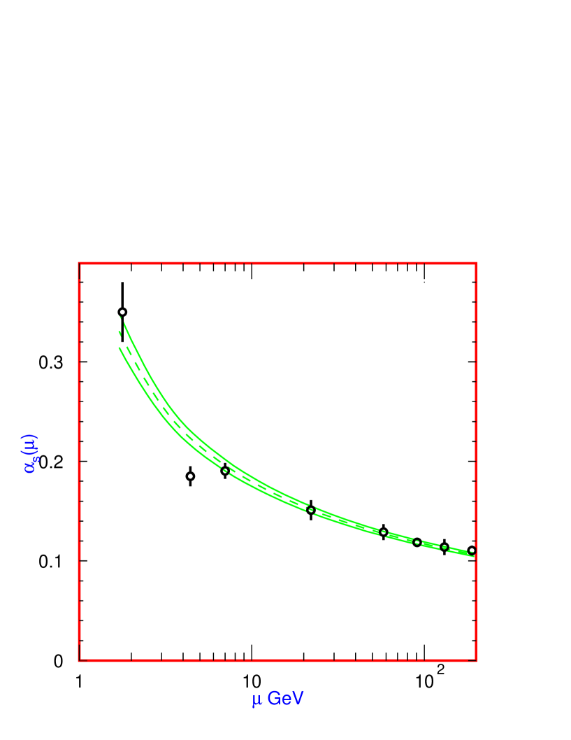
Figure 1.2: Strong coupling constant as a function of energy [2].

Historically, the idea of form factors is related to the ’size’ of subatomic particles, beginning with the determination of nuclear size by Rutherford in alpha scattering experiments. He found that the ’size’ of the nuclei was of the order of 10 fermis. Once it was recognized that the ’size’ should be measured by a probe which itself was ’sizeless’, electron scattering became the means of choice. The concept of form factors was formalized, with the form factor $F(\textbf{q}^{2})$ defined as the multiplicative factor in

$$\left(\frac{d\sigma}{d\Omega}\right)=\left(\frac{d\sigma}{d\Omega}\right)_{point}\times F(\textbf{q}^{2}),$$ (1.8)

where $(d\sigma/d\Omega)_{point}$ is the differential cross section for scattering off a pointlike target and q is the momentum transferred to the target. It can be shown that with this definition the form factor is the Fourier transform of the charge density $\rho(\textbf{r})$

$$F(\textbf{q}^{2})=\int{\mathrm{d}}^{3}{\mathrm{r}}~{}\rho(\textbf{r})~{}{\mathrm{exp}}\left(i~{}\frac{\textbf{q}\cdot\textbf{x}}{\hbar}\right).$$ (1.9)

For small momentum transfers, $F(\textbf{q}^{2})$ only measures the ’size’, or rms radius, of the charge distribution. The classic experiments of Hofstadter and colleagues at Stanford [8, 9] showed that for large momentum transfers considerable more details of the charge and current distributions of the nuclei could be obtained.

The first measurements of electron scattering by nucleons were made by Hofstadter and colleagues at Stanford [10, 11] and by Wilson and colleagues at Cornell [12]. Since then, many more measurements, with much larger momentum transfers and higher precision, have been made. Most of these are electron elastic scattering measurements in which the momentum transfer is spacelike. Since the advent of the $e^{+}e^{-}$ colliders, measurements in which a $h\overline{h}$ pair ($h$ = hadron) is produced in an $e^{+}e^{-}$ annihilation have also been reported. In these measurements, momentum transfer is timelike. However, these measurements have been generally confined to small momentum transfers and have poorer precision. We describe these in detail in the following.

In the commonly used metric, momentum transfers are defined as

$$Q^{2}=-q^{2}=t=(p_{1}-p_{2})^{2},~{}~{}~{}~{}~{}~{}\mathrm{spacelike}~{}Q^{2}$$

$$-Q^{2}=q^{2}=s=(p_{1}+p_{2})^{2},~{}~{}~{}~{}~{}\mathrm{timelike}~{}Q^{2}$$ (1.10)

where the subscripts 1 and 2 refer to the colliding particles and $q$ and $p_{i}$ are four-momenta. For protons, the differential cross section for the timelike momentum transfer, $|Q^{2}|=s$, is described in terms of two form factors, $F^{P}_{1}(s)$ and $F^{P}_{2}(s)$, by [13]

$$\frac{d\sigma}{d\Omega}=\frac{\alpha^{2}\beta_{p}}{4s}~{}[~{}|F^{P}_{1}(s)+\kappa_{p}F^{P}_{2}(s)|^{2}(1+\mathrm{cos}^{2}\theta)~{}~{}~{}~{}~{}~{}~{}~{}~{}~{}~{}~{}~{}~{}~{}~{}~{}~{}~{}~{}~{}$$

$$~{}~{}~{}~{}~{}~{}~{}~{}~{}~{}~{}~{}~{}~{}~{}+\left(\frac{4m^{2}_{p}}{s}\right)\left|F^{P}_{1}(s)+\left(\frac{s}{4m^{2}_{p}}\right)\kappa_{p}F^{P}_{2}(s)\right|^{2}\mathrm{sin}^{2}\theta~{}],$$ (1.11)

where $\beta_{p}$ is the proton velocity measured in the center-of-mass system of the annihilation, $\kappa_{p}$ is the anomalous magnetic moment of the proton, $m_{p}$ is the mass of the proton, and $\theta$ is the angle between the incident positron and the produced proton. The form factor $F^{P}_{1}(s)$ is called the Dirac form factor and relates to both the electric and magnetic scattering from a spin-1/2 Dirac particle, and $F^{P}_{2}(s)$, called the Pauli form factor, is related to the additional magnetic scattering contribution arising from the anomalous part of the proton magnetic moment. It has become conventional to use the so-called Sachs form factors $G^{P}_{E}(s)$ and $G^{P}_{M}(s)$ instead of $F^{P}_{1}(s)$ and $F^{P}_{2}(s)$, with

$$G^{P}_{E}(s)=F^{P}_{1}(s)+\left(\frac{s}{4m^{2}_{p}}\right)\kappa_{p}F^{P}_{2}(s)~{}~{}~{}~{}~{}~{}~{}~{}G^{P}_{M}(s)=F^{P}_{1}(s)+\kappa_{p}F^{P}_{2}(s),$$ (1.12)

so that

$$\frac{d\sigma}{d\Omega}=\frac{\alpha^{2}\beta_{p}}{4s}[~{}|G^{P}_{M}(s)|^{2}~{}(1+\mathrm{cos}^{2}\theta)+\left(\frac{4m^{2}_{p}}{s}\right)|G^{P}_{E}(s)|^{2}~{}\mathrm{sin}^{2}\theta~{}].$$ (1.13)

The normalization is done at $Q^{2}=0$, with

$$F^{P}_{1}(0)=1,~{}~{}~{}~{}~{}F^{P}_{2}(0)=1,~{}~{}~{}~{}~{}~{}~{}~{}~{}~{}~{}~{}~{}~{}~{}~{}~{}~{}\mathrm{and}$$

$$G^{P}_{E}(0)=1,~{}~{}~{}~{}~{}G^{P}_{M}(0)=1+\kappa_{p}=\mu_{p}=2.79,$$ (1.14)

where $\mu_{p}$ is the magnetic moment of the proton in units of the nuclear magneton.

For spin-0 charged mesons, e.g., the pion and kaon, there is no magnetic scattering and only the electric form factor survives, with [13]

$$\frac{d\sigma}{d\Omega}(e^{+}e^{-}\rightarrow m^{+}m^{-})=\frac{\alpha^{2}}{8s}~{}\beta^{3}_{m}~{}|F_{m}(s)|^{2}~{}\mathrm{sin}^{2}\theta,$$ (1.15)

where the $\beta^{3}_{m}~{}\mathrm{sin}^{2}\theta$ dependence is a direct consequence of the fact that the meson pair must be produced in a p-wave state. The normalization is

$$F_{m}(0)=1.$$ (1.16)

The earliest attempts to understand electromagnetic form factors were in terms of the Vector Dominance Model (VDM). In VDM it is assumed that the photon (from $e^{+}e^{-}$ annihilation, for example) ’converts’ into a vector meson, and the vector meson interact hadronically with the hadron whose electromagnetic structure is being probed. The model was originally invented to understand the relation between $\rho\rightarrow e^{+}e^{-}$ and $\rho\rightarrow\pi^{+}\pi^{-}$, and therefore the pion form factor near the mass of the $\rho$ meson [14]. It was later extended to larger energies by including known and hypothesized recurrences of the $\rho$ and $\phi$ mesons [15, 16]. Examples of recent extensions of VDM are Ref. [17] and Ref. [18]. The VDM calculations of the form factors cannot be called predictions; they are fits to the existing experimental data at relatively low momentum transfers, and involve a large number of parameters (32 and 15 for the pion form factor predictions in Ref. [17] and Ref. [18], respectively, and 26 for the kaon form factor prediction in Ref. [18]). The available data in the large momentum transfer region has been either non-existent or of very poor quality, as discussed later. It is worth noting that in the limit of flavor SU(3) invariance, $F_{\pi}(s)=F_{K}(s)$, and attempts to take account of SU(3) breaking do not lead to any large deviations from this [18, 19]. In this dissertation we will not discuss VDM predictions any further, and will concentrate on QCD-based models for form factors.

The earliest attempts to describe the $Q^{2}$ variation of the electromagnetic form factors in terms of QCD were made by Brodsky and Farrar [20, 21] and Matveev, Muradyan, and Tavkhelidze [22]. Their ’dimensional scaling’ considerations lead to the prediction that exclusive scattering scales as $s^{2-n}$, where $n$ is the total number of leptons, photons, and quark components, i.e., elementary fields, in the initial and final states. This directly leads to the so-called ’quark counting rule’ prediction that

$$F_{h}(Q^{2})\sim(Q^{2})^{1-n_{q}},$$ (1.17)

where $n_{q}$ is the number of quarks contained in the hadron. Thus, the form factor for pions and kaons ($n_{q}$ = 2) scales as

$$F_{\pi,K}(Q^{2})\sim(Q^{2})^{-1}$$ (1.18)

and the proton ($n_{q}$ = 3) scales as

$$G^{P}_{E}(Q^{2})=G^{P}_{M}(Q^{2})\sim(Q^{2})^{-2}.$$ (1.19)

It is important to remember that ’dimensional scaling’ or the ’quark counting rule’ is strictly valid only for $|Q^{2}|=s\rightarrow\infty$.

Farrar and Jackson [23] obtained the same $Q^{2}$ behavior for the pion form factor by solving the light-cone pion Bethe-Salpeter equation in QCD, with the additional result relating $F_{\pi}(Q^{2})$ to the pion decay constant. Lepage and Brodsky [24] obtained the same result in a more systematic analysis of PQCD with the ’factorization’ hypothesis. In this model, exclusive processes can be described in terms of two factorizable parts - a necessarily nonperturbative part involving the wave functions of the initial and final states of the hadron and a hard scattering part which can be described perturbatively. The latter leads to both the ’quark counting rule’ behavior and the connection of the $\pi$ and $K$ form factors to their decay constants. The result is that asymptotically ($Q^{2}\rightarrow\infty$) the pion and kaon form factor are

$$Q^{2}~{}F_{\pi,K}(Q^{2})\rightarrow 8\pi~{}\alpha_{s}(Q^{2})~{}f^{2}_{\pi,K},$$ (1.20)

where $f_{\pi}$ = 130.7 $\pm$ 0.4 MeV [2] is the pion decay constant, and $f_{K}$ = 159.8 $\pm$ 1.5 MeV [2] is the kaon decay constant. This prediction gives an absolute normalization to the pion and kaon form factor. For the proton, the asymptotic behavior of the magnetic form factor, neglecting leading logarithms, is

$$Q^{4}~{}G^{P}_{M}(Q^{2})\rightarrow C~{}\alpha^{2}_{s}(Q^{2}),$$ (1.21)

where $C$ is an arbitrary constant. This prediction is not absolutely normalized but it does contain the $\sim$ $Q^{-4}$ behavior predicted by the ’quark counting rule’. It was argued [24] that these predictions were consistent with the then existing form factor data for $Q^{2}>5$ GeV².

Objections have been raised that the above predictions can not applied to the existing data because, at the available momentum transfers, the asymptotic regime has not been reached. Isgur and Llewellyn Smith [25, 26] and Radyushkin [27] have argued that the perturbative part of the form factor can only describe $\sim$10$\%$ of the cross sections and that the other 90$\%$ is dominated by nonperturbative, or ’soft’, processes. A more detailed description of theoretical considerations of the electromagnetic form factors are given in Chapter 2.

The experimental data for the charged pion electromagnetic form factor with timelike and spacelike momentum transfers are shown in Figure 1.3. The spacelike pion form factor is measured using two different techniques. The first, and cleaner, method is by elastically scattering charged pions off electrons bound in atomic targets through the reaction

$$\pi^{-}~{}e^{-}\rightarrow\pi^{-}~{}e^{-}.$$ (1.22)

This method is limited to the determination of the charged radius of the pion because of the very small momentum transfers which can be achieved. For example, even with a 300 GeV beam, $Q^{2}$(max) = 0.12 GeV² was realized [38]. The second method is by pion production off nucleons in the reactions

$$e^{-}~{}p\rightarrow~{}e^{-}~{}\pi^{+}~{}n,$$

$$e^{-}~{}n\rightarrow~{}e^{-}~{}\pi^{-}~{}p.$$ (1.23)

The incoming electron in these reactions emits a virtual photon and the virtual photon interacts with the ’pion cloud’ surrounding the nucleon. The Feynman diagram governing the lowest order process is shown in Figure 1.4. Pion electroproduction for the form factor determination, first proposed by Frazer [45], has recently come under considerable criticism. Carlson and Milana [47] and others [46] have pointed out that the electromagnetic form factor of the pion is not well determined from electroproduction experiments. The concerns arise due to the magnitude of the pion-nucleon form factor, the other competing uncalculated QCD processes, and the inability of many measurements to separate the transverse and longitudinal parts of the measured cross section. The uncertainties in the pion form factor measured from electroproduction experiments range from $\pm 23\%$ to $\pm 51\%$ for $Q^{2}>$ 3 GeV² [42].

Figure 1.3: Experimental status of the charged pion electromagnetic form factor for timelike (top) and spacelike (bottom) momentum transfers. The solid points in the top plot are measurements where $\pi^{+}\pi^{-}$ events are positively observed [28]-[33]. The open points in the top plot are measurements where $\pi^{+}\pi^{-}$ and $K^{+}K^{-}$ events are observed and VDM predictions are used to determine the number of $\pi^{+}\pi^{-}$ events [34]. Results are only shown in the region $|Q^{2}|>$ 1.37 GeV² in the top plot as to exclude the $\rho$ resonance. The solid points in the bottom plot are from $\pi-e$ scattering experiments [35]-[38] and the open triangles are from experiments using electroproduction of charged pions [39]-[43]. The dashed lines in the top and bottom plot are the PQCD predictions by Brodsky $\it{et~{}al.}$ [44] and Lepage and Brodsky [24], respectively.

Figure 1.4: Feymann diagram for electroproduction of charged pions.

The determination of the pion form factor in the timelike region has different problems. The timelike form factor is measured in the reaction

$$e^{+}e^{-}\rightarrow\pi^{+}\pi^{-},$$ (1.24)

and it is theoretically a well defined reaction [13]. However, because of the experimental problems, no direct measurements of the pion form factor are available with $|Q^{2}|$ $>$ 4.5 GeV². In the only existing measurements for $|Q^{2}|$ $>$ 4.5 GeV² meson pairs ($\pi^{+}\pi^{-}$ and $K^{+}K^{-}$) were observed, but it was not possible to individually identify the $\pi^{+}\pi^{-}$ events [34]. The pion form factors were determined using VDM predictions, as described earlier, to divide the number of observed meson pair events into an approximately equal number of $\pi^{+}\pi^{-}$ and $K^{+}K^{-}$ events. Without considering the effect of using a theoretical model to determine form factors, the uncertainties in the measurements are by themselves quite large, $\pm$41$\%$ at $|Q^{2}|$ = 6.76 GeV² and $\pm$100$\%$ with $|Q^{2}|>$ 7 GeV².

The experimental data for the charged kaon electromagnetic form factor with timelike and spacelike momentum transfers are shown in Figure 1.5. As for the pion form factor, the kaon form factor in the spacelike region is measured by elastically scattering charged kaons from electrons bound in atomic targets through the reaction

$$K^{-}~{}e^{-}\rightarrow K^{-}~{}e^{-}.$$ (1.25)

The highest $Q^{2}$ for spacelike momentum transfer is 0.115 GeV², and it is used only to determine the kaon charge radius. The form factor in the timelike region is measured in the reaction

$$e^{+}e^{-}\rightarrow K^{+}K^{-}.$$ (1.26)

As with the pion form factor, no direct measurements of the kaon form factor are available with $|Q^{2}|$ $>$ 4.5 GeV². Only one measurement exists above $|Q^{2}|$ $>$ 4.5 GeV², and once again, the experiment observed meson pairs ($\pi^{+}\pi^{-}$ and $K^{+}K^{-}$) but was not able to individually identify $K^{+}K^{-}$ events [19]. The kaon form factors were determined using VDM predictions to divide the total number of observed hadronic pair events (2 to 8 events) into 1 and 4 events of $K^{+}K^{-}$ [19].

Figure 1.5: Experimental status of the charged kaon electromagnetic form factor for timelike (top) and spacelike (bottom) momentum transfers. The solid points in the top plot are measurements where $K^{+}K^{-}$ events are positively observed [28]-[30], [48]-[51]. The open points in the top plot are measurements where $\pi^{+}\pi^{-}$ and $K^{+}K^{-}$ events are observed and VDM predictions were used to determine the number of $K^{+}K^{-}$ events [19]. Results are only shown in the region $|Q^{2}|>$ 1.28 GeV² in the top plot as to exclude the $\phi$ resonance. The solid points in the bottom plot are data from $K-e$ scattering experiments [52, 53]. The vertical dotted line in the top plot represents the $K^{+}K^{-}$ production threshold ($|Q^{2}|=(2m_{K})^{2}$ = 0.975 GeV²).

The experimental data for the proton electromagnetic form factor is shown in Figure 1.6. As shown in Eqn. 1.13, for large $Q^{2}=s$, $G^{P}_{M}(Q^{2})$ overwhelms $G^{P}_{E}(Q^{2})$, and it becomes impossible to separately measure the electric form factor $G^{P}_{E}(Q^{2})$ and the magnetic form factor $G^{P}_{M}(Q^{2})$. In the results shown in Figure 1.6, $G^{P}_{E}(Q^{2})$ = $G^{P}_{M}(Q^{2})/\mu_{p}$ is assumed. The proton magnetic form factor in the spacelike region has been measured up to $Q^{2}$ = 31.2 GeV² with an uncertainty of $\sim$10$\%$ from elastically scattering electrons off proton targets [71]

$$e^{-}~{}p\rightarrow e^{-}~{}p.$$ (1.27)

$G^{P}_{E}(Q^{2})$ and $G^{P}_{M}(Q^{2})$ separation was done only for $Q^{2}<$ 8.83 GeV² using the Rosenbluth technique. In the timelike region, the proton form factors are measured by $e^{+}e^{-}$ annihilation

$$e^{+}e^{-}\rightarrow p\overline{p},$$ (1.28)

and in the time-reversed $p\overline{p}$ annihilation to the $e^{+}e^{-}$ final state

$$p\overline{p}\rightarrow e^{+}e^{-}.$$ (1.29)

The highest energy measurement from direct $e^{+}e^{-}$ annihilations is $|Q^{2}|$ = 9.42 GeV² and has a 22$\%$ uncertainty [61], while measurements from $p\overline{p}$ annihilations go up to $|Q^{2}|$ = 13.11 GeV² with a 14$\%$ uncertainty [64]. Recently, a BaBar experiment has reported measurement of the proton from factor from $e^{+}e^{-}$ annihilation produced via initial state radiation [62] in the reaction

$$e^{+}e^{-}\rightarrow\gamma(e^{+}e^{-})\rightarrow\gamma(p\overline{p}).$$ (1.30)

They were able to measure the timelike form factor up to $|Q^{2}|$ $\sim$ 20 GeV² but with uncertainties between $\pm 40\%$ and $\pm 100\%$ in large $Q^{2}$ bins. Figure 1.6 also shows that, at the present momentum transfers, the timelike form factor is approximately twice as large as the spacelike form factor.

Figure 1.6: Experimental status of the proton magnetic form factor for timelike (top) and spacelike (bottom) momentum transfers. The solid points for timelike momentum transfer are from Refs. [54]-[62], while the stars are the E760/E835 measurements from $p\overline{p}\rightarrow e^{+}e^{-}$ events [63]-[65]. The timelike data assumes $|G^{P}_{E}(Q^{2})|$ = $|G^{P}_{M}(Q^{2})|$. The data points for spacelike momentum transfer are from Refs. [66]-[71] assuming $G^{P}_{E}(Q^{2})$ = $G^{P}_{M}(Q^{2})/\mu_{p}$. The vertical dotted line in the top plot represents the $p\overline{p}$ production threshold ($|Q^{2}|=(2m_{p})^{2}$ = 3.52 GeV²). The dashed lines are the arbitrarily-normalized PQCD prediction $|Q^{4}||G^{P}_{M}(Q^{2})|\propto\alpha^{2}_{s}(|Q^{2}|)$ [24].

The $G^{P}_{E}(Q^{2})/G^{P}_{M}(Q^{2})$ ratio for the proton has been measured in the spacelike region with $Q^{2}<$ 9 GeV² using two different methods, Rosenbluth separation and polarization transfer. The differential cross section for Rosenbluth separation [72] is

$$\left(\frac{d\sigma}{d\Omega}\right)_{exp}=\left(\frac{d\sigma}{d\Omega}\right)_{point}\times\left(~{}\frac{[G^{P}_{E}(Q^{2})]^{2}+\tau[G^{P}_{M}(Q^{2})]^{2}}{1+\tau}+2\tau[G^{P}_{M}(Q^{2})]^{2}~{}\mathrm{tan}^{2}\frac{\theta_{e}}{2}~{}\right),$$ (1.31)

where $\tau$ = $\frac{Q^{2}}{4m^{2}_{p}}$ and $\theta_{e}$ is defined as the angle between the incident and scattered electron. Precision measurements of $G^{P}_{E}(Q^{2})$ in Rosenbluth separation experiments are limited because the overall cross section becomes less sensitive to it with increasing momentum transfer. The measurements using polarization transfer consist of elastically scattering of polarized electrons off proton targets. Scattering of longitudinally polarized electrons off unpolarized proton targets gives the recoiling proton either polarization transverse to ($P_{t}$), or in the same longitudinal direction ($P_{l}$), of the recoiling proton, with respect to the scattering plane defined by the incident electron and the recoiling proton. The $G^{P}_{E}/G^{P}_{M}$ ratio at a given $Q^{2}$ is determined in the polarization transfer experiments as [73, 74]

$$\frac{G_{E}}{G_{M}}=\frac{P_{t}}{P_{l}}\frac{E+E^{\prime}}{2m_{p}}\mathrm{tan}\frac{\theta_{e}}{2},$$ (1.32)

where $E$ and $E^{\prime}$ are the energies of the incident and scattered electron, respectively. The results are shown in Figure 1.7, where the ratio is plotted as $\mu_{p}G^{P}_{E}(Q^{2})/G^{P}_{M}(Q^{2})$.

Figure 1.7: Experimental results for the ratio $\mu_{p}G^{P}_{E}(Q^{2})/G^{P}_{M}(Q^{2})$ in the timelike (top) and spacelike (bottom) regions. Top: The solid points are the experimental results from Ref. [62]. The vertical dotted line in the top plot represents the $p\overline{p}$ production threshold ($|Q^{2}|=(2m_{p})^{2}$ = 3.52 GeV²). Bottom: The open squares are from the polarization transfer [88]-[91] measurements, and the solid points are from the Rosenbluth separation [75]-[87] measurements. Note that the polarization transfer results show a monotonic decrease in the ratio, while the Rosenbluth results are all consistent with the ratio being constant $\approx$ 1.

As shown in Figure 1.7, $\mu_{p}G^{P}_{E}(Q^{2})/G^{P}_{M}(Q^{2})$ measured by the polarization transfer experiments differs from those using Rosenbluth separation. The ratio determined from Rosenbluth separation is consistent with the electric and magnetic form factors being equal, or $G^{P}_{E}(Q^{2})$ = $G^{P}_{M}(Q^{2})/\mu_{p}$, while the ratio from polarization transfer decreases linearly. A linear extrapolation of the polarization transfer measurements would lead to $G^{P}_{E}$ = 0 at $Q^{2}$ $\sim$ 7.5 GeV². The only measurement of the electric-to-magnetic form factor ratio in the timelike region is from the BaBar experiment [62], which measures the angular distribution of $p\overline{p}$ events produced in $e^{+}e^{-}$ annihilations via initial state radiation. As shown in Figure 1.7, BaBar finds that the ratio in the $|Q^{2}|$ range 4.4$-$9.0 GeV² is consistent with $|G^{P}_{E}(Q^{2})|/|G^{P}_{M}(Q^{2})|$ = 1, which is predicted by Eqn. 1.12 for the $p\overline{p}$ threshold condition, $|Q^{2}|=s=4m_{p}^{2}$. The form factor ratio in the timelike region is also given by Eqn. 1.13, and therefore it contains the same sensitive issue for extracting $|G^{P}_{E}(Q^{2})|$ by the Rosenbluth separation method.

We have used the data collected with the CLEO detector at the Laboratory of Elementary Particle Physics in Ithaca, NY, to measure the electromagnetic form factors of the charged pion, charged kaon, and proton with timelike momentum transfer. The Cornell Electron Storage Ring (CESR) began colliding $e^{+}e^{-}$ beams in 1979 at a center-of-mass energy of $\sqrt{s}\sim$ 10 GeV. The original CLEO detector, CLEO I, was constructed to study quarkonium spectroscopy by means of $e^{+}e^{-}$ annihilations. The CLEO I detector was upgraded to CLEO II, CLEO II.V, and CLEO III between 1979 and 2003. In 2003, CESR was redesigned to run in the lower energy region of $\sqrt{s}$ = 3-5 GeV, and the CLEO III detector was modified to the present CLEO-c detector.

The CLEO-c detector collected 20.7 pb^-1 of $e^{+}e^{-}$ annihilation data at a center-of-mass energy $\sqrt{s}$ = 3.671 GeV, or $|Q^{2}|$ = 13.48 GeV², between January and April of 2004. This data sample is used in this dissertation to measure the timelike electromagnetic form factors of the charged pion, charged kaon, and proton at $|Q^{2}|$ = 13.48 GeV².

Before presenting the results of our measurements, in Chapter 2, we discuss the current theoretical interpretations of the electromagnetic form factors. In Chapter 3 we describe the Cornell Electron Storage Ring and the CLEO-c detector used to produce and observe the $e^{+}e^{-}$ annihilations to the exclusive final states $\pi^{+}\pi^{-}$, $K^{+}K^{-}$, and $p\overline{p}$. In Chapter 4 we describe our measurements and the analysis procedure for determining the respective electromagnetic form factors. Finally, in Chapter 5 we summarize the experimental results and compare them to existing experimental results and theoretical predictions. We conclude by discussing the impact of our measurements on the validity of applying PQCD at $|Q^{2}|$ $\sim$ 10 GeV². Appendix A lists the individual event properties for events which satisfy the $e^{+}e^{-}\rightarrow\pi^{+}\pi^{-}$ and $e^{+}e^{-}\rightarrow p\overline{p}$ selection criteria. Appendix B lists the existing experimental results of the pion, kaon, and proton form factors used throughout this dissertation.

Chapter 2 Form Factors - Theoretical

In this chapter I review the present status of the theoretical understanding of the electromagnetic form factors of hadrons. As always, the development of theoretical models is closely related to the availability of experimental data. Unfortunately the available experimental data for $\pi$, $K$, and $p$ are limited in two ways. Very little data are available for timelike or spacelike form factors for large momentum transfers
($>$ 5 GeV²), and the few data which are available generally suffer from very large, up to $\pm$100$\%$, uncertainities. Because of these limitations theoretical models have generally concentrated on $Q^{2}\lesssim 2$ GeV² and for spacelike momentum transfers.

In the following review, the theoretical developments are organized in the following manner. As stated in Chapter 1, I confine myself here to the developments in the framework of Quantum Chromodynamics (QCD) and do not discuss pure Vector Dominance Models (VDM) related predictions. Within the framework of QCD I discuss the basic ideas of the three prevalent approaches: (1) Factorization based Perturbative QCD, (2) QCD sum rules, and (3) Lattice QCD. These considerations apply to all hadrons, including $\pi$, $K$, and $p$. The presentation is then divided in two parts, pseudoscalar mesons ($\pi$ and $K$) and baryons ($p$). I discuss theoretical predictions for pion form factors since nearly all meson form factor predictions relate to pions, but I note that, in general, the theoretical models can be extended to kaons, although explicit predictions are few. I conclude with the proton form factor.

2.1 Theoretical Formalisms

Different theoretical predictions interpret the photon-hadron vertex in different ways. Figure 2.1 shows the Feymann diagrams for the photon-hadron interactions for spacelike and timelike momentum transfers. The most fundamental theories are based on the modern quantum field theory describing the strong interaction, Quantum Chromodynamics (QCD). They attempt to describe the behavior of the strong interaction between quarks within the hadron. At large momentum transfers, the strong interaction can be described through a power series expansion in terms of the strong coupling constant, $\alpha_{s}(Q^{2})$. This procedure is known as Perturbative Quantum Chromodynamics (PQCD) and its complete formalism for hadronic form factors has been described by Lepage and Brodsky [24] in 1980.

Figure 2.1: Feymann diagrams for studying the electromagnetic form factors of a hadron. Left: Spacelike momentum transfer from electron scattering. The initial and final four-momenta of the electron are $p_{1}$ and $p_{2}$, respectively. The initial and final four-momenta of the hadron are $k_{1}$ and $k_{2}$, respectively. The four-momentum of the virtual photon is defined as $Q^{2}=-q^{2}=t=(p_{1}-p_{2})^{2}$. Right: Timelike momentum transfer from $e^{+}e^{-}$ annihilations. The initial four-momenta of the electron and positron are $p_{1}$ and $p_{2}$, respectively. The final four-momenta of the hadron and ’anti’hadron are $k_{1}$ and $k_{2}$, respectively. The four-momentum of the virtual photon is defined as $-Q^{2}=q^{2}=s=(p_{1}+p_{2})^{2}$

.

2.1.1 Factorization

Figure 2.2 shows the PQCD factorization scheme diagrams associated with elastic pion scattering by a virtual photon. The incoming pion has a momentum $p_{1}$. The probability that it will be in a state consisting of two collinear quarks carrying momenta $x_{1}p_{1}$ and $x_{2}p_{1}$ (where $x_{i}$ is the momentum fraction of the $i$th quark, satisfying $\Sigma_{i}x_{i}=1$) is given by distribution amplitude $\phi_{\pi}$. One of the quarks is struck by the photon carrying momentum $q$. A portion of the momentum absorbed by the struck quark must be distributed to the other quark in order for the two quarks to remain bound together. The momentum is exchanged through the emission of gluons. To the lowest order, as shown on the bottom of Figure 2.2, this is done by through the exchange of a single hard gluon. The transfer of momentum by the gluon redistributes the momenta carried by the quarks, which are represented by $y_{1}p_{2}$ and $y_{2}p_{2}$ (where $y_{i}$ is the momentum fraction carried by the final state quarks). The probability that the two valence quarks will come out collinear and reform a pion with momentum $p_{2}=p_{1}+q$ is given by the distribution amplitude $\phi^{*}_{\pi}$.

Figure 2.2: PQCD factorization diagrams for the pion. The top figure shows the pion approaching from the left in the form of the initial pion distribution amplitude ($\phi_{\pi}$), the virtual photon interacting with the pion (T_H), and the final pion distribution amplitude ($\phi^{\ast}_{\pi}$) of the outgoing pion. The bottom figure shows the leading order terms for the hard scattering amplitude (T_H). The crosses represent the quark-photon interaction.

The central feature of applying QCD based perturbation theory to the description of the form factor is the separation of the process into the perturbative and the nonperturbative parts. The photon-pion interaction, denoted by $T_{H}$, probes the short-distance aspect of the pion. The scale of this interaction is set by the momentum transfer of the photon, $Q^{2}=q^{2}$. If the momentum transfer is large enough, the strong coupling constant associated with the gluon transferring momentum (which is on the order of $Q^{2}$) to the spectator quark will be small (see Eqn. 1.7 for the momentum dependence of $\alpha_{s}(Q^{2})$). Hence, $T_{H}$ can be described within PQCD. The probability of finding the pion with two valence quarks is given by the distribution amplitude. It is governed by long-distance QCD and has to be treated nonperturbatively.

For the general case of a given hadron, the form factor is expressed in the factorized PQCD scheme by [24]

$$F(Q^{2})=\int^{1}_{0}\int^{1}_{0}[dx][dy]~{}\phi^{\ast}(y_{i},Q^{2})~{}T_{H}(x_{i},y_{i},Q^{2},\mu^{2}_{R})~{}\phi(x_{i},Q^{2}),$$ (2.1)

where the hard scattering amplitude is denoted by $T_{H}(x_{i},y_{i},Q^{2},\mu^{2}_{R})$, the incoming and outgoing hadron distribution amplitudes are denoted by $\phi(x_{i},Q^{2})$ and $\phi^{\ast}(y_{i},Q^{2})$, respectively, and $\mu^{2}_{R}$ is the renormalization scale of the strong coupling constant, $\alpha_{s}(\mu^{2}_{R})$. The subscript $i$ is defined by the number of constituent quarks (i.e., $i$ = 2 for mesons and $i$ = 3 for baryons). The integration variable of the quark momentum fraction is $[dx]\equiv(\sum_{i}dx_{i})~{}\delta(1-\Sigma_{i}x_{i})$ and the same for $[dy]$.

Any prediction of a physical process using perturbation theory needs to be independent of the renormalization scale. For a given process, the ideal procedure is to evaluate every term in the $\alpha_{s}(\mu^{2}_{R})$ power series expansion. This is nearly impossible because more complicated contributions arise at higher orders, and therefore the power series must be truncated. The general form of the power expansion of the form factor in $\alpha_{s}(\mu^{2}_{R})$ is

$$F(Q^{2},\mu^{2}_{R})=\alpha_{s}(\mu^{2}_{R})F^{(0)}(Q^{2},\mu^{2}_{R})[~{}1+\alpha_{s}(\mu^{2}_{R})F^{(1)}(Q^{2},\mu^{2}_{R})+\cdots],$$ (2.2)

where $F^{(0)}(Q^{2},\mu^{2}_{R})$ is the leading order (LO) contribution, $F^{(1)}(Q^{2},\mu^{2}_{R})$ is the next-to-leading (NLO) contribution, and higher order contributions are represented by the dots. The truncation of the series is determined by the renormalization scale, $\mu^{2}_{R}$. The renormalization scale setting is important for an exclusive process like the form factor of the hadron. In the following discussions it will be set by the momentum transfer of the virtual photon, $\mu^{2}_{R}=Q^{2}$, unless otherwise specified.

The value of $\alpha_{s}(Q^{2})$ determines the validity of applying perturbation theory. The behavior of $\alpha_{s}(Q^{2})$ at low $Q^{2}$ is not only large but is undefined when $Q^{2}$ = $\Lambda^{2}$, a.k.a. the Landau pole. One possible method to avoid this behavior is to ’freeze’ the value of $Q^{2}$ by introducing an effective gluon mass. Originally proposed by Parisi and Petronzio [92] and Cornwall [93], the ’frozen’ version of $\alpha_{s}(Q^{2})$ modifies the one loop form of $\alpha_{s}(Q^{2})$ (given by Eqn. 1.7) into [93]

$$\alpha_{s}(Q^{2})=\frac{4\pi}{\beta_{0}~{}\mathrm{ln}\left(\frac{Q^{2}+4m^{2}_{g}}{\Lambda^{2}}\right)},$$ (2.3)

where $m^{2}_{g}$ is the effective gluon mass. This definition of $\alpha_{s}(Q^{2})$ freezes its value in the range $Q^{2}<4m^{2}_{g}$. For larger values of $Q^{2}$, the gluon mass has a small and negligible effect on $\alpha_{s}(Q^{2})$, and this modification is not relevant.

2.1.2 QCD Sum Rules

The QCD sum rule (QCDSR) approach is based on the pioneering work of Shifman, Vainshtein, and Zakharov [94]. Its premise is that the properties of a hadron are dictated by its interactions with the QCD vacuum, composed of violent fluctuations of virtual gluons ($G^{a}_{\mu\nu}G^{a}_{\mu\nu}$) and quark-antiquark pairs ($q\overline{q}$). These interactions are governed by the nonperturbative aspects of QCD.

The relationship between the hadron and the QCD vacuum is described in terms of the operator product expansion of hadronic currents, which consist of the constituent quarks of the hadron of interest. Its explicit form is expressed in terms of time ordered hadronic currents $j_{1}$ and $j_{2}$ by [94]

$$i\int d^{4}x~{}\mathrm{e}^{iqx}\langle 0|~{}T[j_{2}(x)j_{1}(0)]~{}|0\rangle=\sum_{n}C^{12}_{n}(q)O_{n},$$ (2.4)

where $q$ and $x$ are the momentum and position of the hadron current $j_{2}$ with respect to the current $j_{1}$. The interactions between the QCD vacuum and the hadrons are described by local field operators, $O_{n}$, and their coefficients, $C^{12}_{n}(q)$. The operators are defined by their twist, where twist is defined as the canonical dimension of the operator minus its spin. Higher twist operators describe higher order interactions between the hadronic currents and the QCD vacuum.

Each hadronic current in Eqn. 2.4 has a characteristic energy scale defined by $s_{i}$ , which has units of energy squared ($i=1,2$ are with respect to the hadronic currents $j_{1}$ and $j_{2}$, respectively). There is a corresponding energy threshold, denoted as $s_{0}$, which is the maximum energy for which the quarks that comprise the current can be associated with the hadron of interest (e.g., $\pi$, $K$, $p$). For energies above $s_{0}$, the currents are contaminated by higher resonance states with the same quark structure. This energy threshold defines the region for the so-called quark-hadron duality [94].

The QCDSR is used in three different ways to determine the electromagnetic form factor of a hadron. They are briefly reviewed below.

The first way is the distribution amplitude moment method. This formalism originates from the work by Chernyak and Zhitnitsky [95]. Here one determines distribution amplitudes based on their moments, which are then used in the PQCD factorization scheme.

In the second way one determines the electromagnetic form factors by using the three-point amplitude method. The initial application of the three-point amplitude in describing of the pion form factor was made independently by Nesterenko and Radyushkin [96] and Ioffe and Smilga [97]. It consists of replacing the matrix element in the left hand side of Eqn. 2.4 by [96]

$$\langle 0|~{}T[j_{\alpha}(y)j^{em}_{\mu}(0)j_{\beta}(x)]~{}|0\rangle,$$ (2.5)

where $j_{\beta}(x)$ and $j_{\alpha}(y)$ are the incident and final state hadron currents and $j^{em}_{\mu}(0)$ is the electromagnetic interaction with one of the quarks. The process is schematically illustrated for pion form factor in Figure 2.3 (left). The incoming pion current with momentum $p_{1}$ breaks into its quark and antiquark representation, the photon interacts with one of the quarks, and the outgoing quarks recombine into a pion current with momentum $p_{2}$.

Two different treatments of the energy scales of the hadronic currents are used with the three-point amplitude method. The first, called the square representation, treats the scales independently, i.e., $0<s_{1}<s_{0}$ and $0<s_{2}<s_{0}$. The other, called the triangle representation, replaces the energy scales in the square representation with a triangle of the same area, i.e., $0<s_{1}+s_{2}<S_{0}=\sqrt{2}~{}s_{0}$.

Figure 2.3: The three-point amplitude and correlator function diagrams used with QCD sum rules for the pion form factor. Left: The three-point amplitude diagram. The four-momenta of the incoming pion current, virtual photon, and outgoing pion current are $p_{1}$, $q$, and $p_{2}$, respectively. Right: The correlator function diagram. The four-momenta of the incoming composite pion, virtual photon, and outgoing pion current are $p_{1}$, $q$, and $p_{2}$, respectively. The quarks are denoted by the single arrowed lines in both cases.

The third way determines the electromagnetic form factors by using the correlator function method. It consists of replacing the matrix element in the left hand side of Eqn. 2.4 by [98]

$$\langle 0|~{}T[j_{\nu}(0)j^{em}_{\mu}(x)]~{}|\pi^{+}(p_{1})\rangle,$$ (2.6)

where the initial pion is described by $|\pi^{+}(p)\rangle$, the final pion by the current $j_{\nu}(x)$, and $j^{em}_{\mu}(0)$ is the electromagnetic interaction with one of the quarks. The process is schematically illustrated for pion form factor in Figure 2.3 (right). The composite incoming pion with momentum $p_{1}$ breaks into its quark and antiquark representation, the photon interacts with one of the quarks, and the outgoing quarks recombine into its pion, described by the hadronic current, with momentum $p_{2}$. The correlator function method can be used to determine distribution amplitudes [98].

2.1.3 Lattice QCD

In 1974, Wilson [5] showed how to quantize a gauge field theory on a discrete lattice in Euclidean space-time preserving exact gauge invariance. He applied this calculational technique to the strong coupling regime of QCD. In these Lattice Gauge calculations (Lattice QCD), space-time is replaced by a four dimensional hypercubic lattice of size $L^{3}T$. The sites are separated by the lattice spacing $a$. The quarks and gluons fields are defined at discrete points. Physical problems are solved numerically by Monte Carlo simulations requiring only the quarks masses as input parameters.

Lattice QCD has been used to calculate the electromagnetic form factor of the hadron (e.g., for the pion form factor, see Ref. [99]) using lattice correlation functions. The correlation functions connect a hadron creation operator at time $t_{i}$, a hadron annihilation operator at $t_{f}$, and a vector current insertion at $t$ ($t_{i}<t<t_{f}$). All of the calculations have so far been performed in the ’quenched’ approximation, in which no virtual quark-antiquark pairs are allowed to be produced from the vacuum.

2.2 Meson Form Factors in Theory

The electromagnetic form factor of a spin-0 meson, studied with spacelike momentum transfers, is related to the following matrix element

$$\langle m(p_{2})|~{}j^{em}_{\mu}~{}|m(p_{1})\rangle=(p_{2}+p_{1})_{\mu}F(Q^{2}),$$ (2.7)

where the electromagnetic current $j^{em}_{\mu}$ = $\Sigma_{f}~{}e_{f}~{}\overline{q}_{f}\gamma_{\mu}q_{f}$ is expressed in terms of quarks $q_{f}$ with flavor $f$ and electric charge $e_{f}$; the spacelike momentum transfer is defined as $Q^{2}$ = $-q^{2}$ = $(p_{1}-p_{2})^{2}$, and $p_{1}$ and $p_{2}$ are the initial and final momenta of the meson, respectively. The form factor $F(Q^{2})$ measures the deviation of the meson from a Dirac point particle. The matrix element for timelike momentum transfers is obtained by replacing $\langle m(p_{2})|~{}j^{em}_{\mu}~{}|m(p_{1})\rangle$ with $\langle m(p_{1})\overline{m}(p_{2})|~{}j^{em}_{\mu}~{}|0\rangle$. The timelike momentum transfer is defined as $-Q^{2}$ = $q^{2}$ = $s$ = $(p_{1}+p_{2})^{2}$, where $s$ is the center of mass energy square of the system, and $p_{1}$ and $p_{2}$ are the momenta of the meson and the ’anti’ meson, respectively.

This section is organized as follows. The pion form factor will be discussed, concentrating mostly on PQCD and QCDSR. The description of the kaon form factor based on PQCD and QCDSR follows. The majority of the theoretical literature is devoted to the discussion of form factors in the spacelike region, and it will be reviewed. Predictions of the form factors in the timelike region are described at the end of each subsection.

2.2.1 Perturbative Quantum Chromodynamics

The formalism for form factor predictions based on the PQCD factorization scheme has been described in Section 2.1.1. The process for the pion form factor is shown schematically in Figure 2.2. The lowest order contribution to the meson form factor is the interaction of a single hard gluon between the two valence quarks. The momentum dependence of the hard gluon propagator is proportional to $1/Q^{2}$. The form factor is therefore $F(Q^{2})\sim 1/Q^{2}$, consistent with the ’quark counting rules’ [20, 21, 22]. Higher order corrections arise from higher Fock, i.e., non-valence, states and other nonperturbative effects, which are suppressed with respect to the single hard gluon exchange.

The formalism for describing the meson form factor by the PQCD factorization scheme was determined independently by Farrar and Jackson [23], Efremov and Radyushkin [100], and Lepage and Brodsky [101]. As described by Eqn. 2.1 in Section 2.1.1., the meson form factor is expressed in the factorized PQCD scheme by

$$F(Q^{2})=\int^{1}_{0}\int^{1}_{0}[dx][dy]~{}\phi^{\ast}(y_{i},Q^{2})~{}T_{H}(x_{i},y_{i},Q^{2},\mu^{2}_{R})~{}\phi(x_{i},Q^{2}),$$ (2.8)

The hard scattering amplitude $T_{H}(x_{i},y_{i},Q^{2},\mu^{2}_{R})$ incorporates the short-distance interactions between the constitute quarks inside the meson. The lowest order contribution from the emission of a single hard gluon is given as [24]

$$T_{H}(x_{i},y_{i},Q^{2},\mu^{2}_{R})=\frac{8\pi~{}C_{F}~{}\alpha_{s}(\mu^{2}_{R})}{Q^{2}}\left[~{}\frac{e_{1}}{x_{2}y_{2}}+\frac{e_{2}}{x_{1}y_{1}}\right],$$ (2.9)

where $e_{1}$ and $e_{2}$ are the electric charges of the quarks and $C_{F}=(n^{2}_{c}-1)/2n_{c}=4/3$ with $n_{c}=3$ denoting the number of colors.

The meson distribution amplitude contains all of the nonperturbative aspects of the interaction. The meson distribution amplitude, $\phi(x_{i},Q^{2})$, is related to the integral of the full meson wave function, $\psi(x_{i},\mathbf{k}_{\perp,i})$, over the transverse momentum $\mathbf{k}_{\perp,i}$ of the $i$th quark by [24]

$$\phi(x_{i},Q^{2})=\int^{Q^{2}}\frac{d^{2}\mathbf{k}_{\perp,i}}{16\pi^{3}}~{}\psi(x_{i},\mathbf{k}_{\perp,i}),$$ (2.10)

The general solution of the distribution amplitude is a series of Gegenbauer polynomials $C^{3/2}_{n}$ [24]

$$\phi(x_{i},Q^{2})=x_{1}x_{2}\sum^{\infty}_{n=0}a_{n}~{}C^{3/2}_{n}(x_{1}-x_{2})[~{}1+O(\alpha_{s}(Q^{2}))~{}],$$ (2.11)

where $a_{n}$ are the coefficients of the polynomial. In the large $Q^{2}$, or asymptotic, limit ($Q^{2}\to\infty$), the first term of the distribution amplitude (Eqn. 2.11) dominates. The distribution amplitude is therefore $\phi^{asy}(x_{i},Q^{2})=a_{0}~{}x_{1}x_{2}$, or $\phi^{asy}(x_{i},Q^{2})=a_{0}~{}x(1-x)$ with the replacements $x_{1}=x$ and $x_{2}=1-x$, and is commonly referred to as the asymptotic distribution amplitude. The quark momentum fraction dependence of the asymptotic distribution amplitude is shown in Figure 2.4.

Figure 2.4: Asymptotic and CZ distribution amplitudes for the pion as a function of quark momentum fraction $x$. The solid line is the asymptotic form (asy: $\phi^{asy}_{\pi}(x)=(f_{\pi}\cdot\sqrt{3/2})x(1-x)$) and the dashed line is the Chernyak-Zhitnitsky form (CZ: $\phi^{CZ}_{~{}\pi}(x)=(f_{\pi}\cdot 15/4)x(1-x)(2x-1)^{2}$). The pion decay constant is taken to be unity in this figure.

For the pion, the normalization of the distribution amplitude is determined from the matrix element between the quark-antiquark pair and the composite pion, i.e., $\langle 0|\overline{d}\gamma_{5}\gamma_{\mu}u|\pi^{+}(p)\rangle$. The $a_{0}$ coefficient in the asymptotic distribution amplitude is fixed by relating it to the weak decay process $\pi^{+}\to\mu^{+}\nu_{\mu}$. This leads to $\langle 0|\overline{d}\gamma_{5}\gamma_{\mu}u|\pi^{+}(p)\rangle$ = $p_{\mu}\sqrt{2/3}~{}a_{0}$ = $p_{\mu}f_{\pi}$, or $a_{0}$ = $\sqrt{3/2}f_{\pi}$, where $f_{\pi}$ = 130.7 $\pm$ 0.4 MeV [2] is the pion decay constant. The asymptotic pion distribution amplitude is therefore [24]

$$\phi^{asy}(x_{i},Q^{2})=\sqrt{3/2}~{}f_{\pi}~{}x_{1}x_{2}$$ (2.12)

Substituting the asymptotic distribution amplitude (Eqn. 2.12) and the hard scattering amplitude (Eqn. 2.9) into the factorization expression (Eqn. 2.8), in the limit of large spacelike momentum transfer, the pion form factor is [24]

$$F_{\pi}(Q^{2})=\frac{8\pi~{}f^{2}_{\pi}~{}\alpha_{s}(Q^{2})}{Q^{2}},$$ (2.13)

or

$$Q^{2}~{}F_{\pi}(Q^{2})=8\pi~{}f^{2}_{\pi}~{}\alpha_{s}(Q^{2})~{}\mathrm{GeV}^{2}=0.43~{}\alpha_{s}(Q^{2})~{}\mathrm{GeV}^{2}.$$ (2.14)

The pion form factor in the large $Q^{2}$ limit is dominated by the hard gluon emission between the valence quarks and is absolutely normalized by the pion decay constant. This result will be referred to as the asymptotic form factor prediction. The spacelike form factor prediction [24] for the pion, as a function of $Q^{2}$, with $\Lambda=0.316$ GeV, is shown in Figure 2.5. It is nearly factor three smaller than the data in the $Q^{2}=1-2$ GeV² range in which the data have reasonable errors.

Figure 2.5: Asymptotic PQCD prediction of the spacelike pion form factor. The line is the PQCD prediction by Lepage and Brodsky with $\Lambda=0.316$ GeV [24]. The solid points and open triangles are experimental data [35]-[43].

Pion distribution amplitudes are also determined from the QCDSR using the distribution amplitude moment method. The moments of the pion distribution amplitude are defined as [95]

$$\langle\xi^{n}\rangle=\int^{1}_{-1}d\xi~{}\xi^{n}~{}\phi(\xi).$$ (2.15)

where $\xi=x_{1}-x_{2}=2x-1$ is the momentum fraction difference between the two valence quarks. By using the QCDSR, the moments are found to be $\langle\xi^{0}\rangle=$ 1, $\langle\xi^{2}\rangle\simeq$ 0.46, and $\langle\xi^{4}\rangle\simeq$ 0.30 [95]. The distribution amplitude, derived by Chernyak and Zhitnitsky [95], which reproduces these moments is

$$\phi^{CZ}_{~{}\pi}(x)=\frac{15}{4}~{}f_{\pi}~{}(1-\xi^{2})\xi^{2}=15~{}f_{\pi}~{}x(1-x)(2x-1)^{2}.$$ (2.16)

This asymmetric double-humped distribution amplitude forces one quark to carry
$\sim$$85\%$ of the pion momentum. Figure 2.4 compares the momentum fraction dependence of the Chernyak-Zhitnitsky (CZ) and asymptotic distribution amplitudes. Using the CZ distribution amplitude in the PQCD factorization scheme results in a spacelike pion form factor prediction which is about five times larger than the prediction from the asymptotic distribution amplitude, as shown in Figure 2.6.

Figure 2.6: PQCD factorization prediction of the spacelike pion form factor using the CZ pion distribution amplitude. The predictions are by Chernyak and Zhitnitsky [95]. The solid line is the prediction using the CZ distribution amplitude, and the dashed is the prediction using the asymptotic distribution amplitude. The solid points and open triangles are experimental data [35]-[43].

Ji and Amiri [102] have calculated the spacelike pion form factor using the CZ distribution amplitude and the ’frozen’ version of $\alpha_{s}(Q^{2})$ (see Eqn. 2.3 for definition of frozen $\alpha_{s}(Q^{2})$). The predictions are similar to those by Chernyak and Zhitnitsky [95], and are in reasonable agreement with the data, as shown in Figure 2.7.

Figure 2.7: PQCD factorization prediction of the spacelike pion form factor using the CZ distribution amplitude and the ’frozen’ version of $\alpha_{s}(Q^{2})$. The predictions are by Ji and Amiri [102]. The solid, dashed, and dotted lines are with $m^{2}_{g}$ = 0.1, 0.3, and 0.5 GeV², respectively. The solid points and open triangles are experimental data [35]-[43].

Arguments have been raised about the validity of the PQCD predictions to describe the existing experimental data. Isgur and Llewellyn Smith [25, 26] have argued that the spacelike form factor prediction with the asymptotic and CZ distribution amplitudes contain significant contributions from regions where most of the momentum of the pion is carried by one quark ($x\approx$ 0 or 1). Near $x\to 0,1$, the gluon virtuality $x_{i}y_{i}Q^{2}$ is small but $\alpha_{s}(x_{i}y_{i}Q^{2}$) is quite large. Therefore PQCD should not be applied in these regions. This issue is called the end-point problem. Isgur and Llewellyn Smith argue that the PQCD form factor prediction should be restricted to regions where the gluon virtuality is above some minimum value so that higher order effects can be appropriately neglected. Table 2.1 lists the percentage of the form factor predictions which arise in the valid region above different momentum transfer cutoffs. As shown in Table 2.1, with a cutoff at $x_{i}y_{i}Q^{2}=$ 1 GeV², the valid part of the PQCD form factor prediction with the asymptotic distribution amplitude is only 2$\%$ at $Q^{2}$ = 2 GeV² and 52$\%$ at $Q^{2}$ = 16 GeV². The situation is even worse for prediction using the CZ distribution amplitude. Isgur and Llewellyn Smith therefore conclude [25, 26] that the form factor at currently accessible energies gets most of its contribution from higher order nonperturbative effects.

Table 2.1: Valid contributions of the pion PQCD form factor predictions using the asymptotic and CZ distribution amplitudes. The values are the percentage of the original PQCD prediction which remains after excluding the end-point regions, defined by the $x_{i}y_{i}Q^{2}$ cutoff. This table is reproduced from Ref. [26].

	$\phi^{asy}_{\pi}(x)$			$\phi^{CZ}_{~{}\pi}(x)$
Cutoff (GeV2)	0.25	0.5	1.0	0.25	0.5	1.0
Q2 (GeV2):
1	13$\%$	2$\%$	0$\%$	2$\%$	1$\%$	0$\%$
2	32$\%$	13$\%$	2$\%$	8$\%$	2$\%$	1$\%$
4	52$\%$	32$\%$	13$\%$	16$\%$	8$\%$	2$\%$
8	68$\%$	52$\%$	32$\%$	27$\%$	16$\%$	8$\%$
16	80$\%$	68$\%$	52$\%$	41$\%$	27$\%$	16$\%$

Li and Sterman [103] extended the PQCD factorization scheme to include effects from the transverse momenta of the quarks. The transverse momenta are suppressed by QCD radiative corrections, the so-called Sudakov effects. Sudakov effects arise from the QCD radiative corrections to the quark propagator and the photon-quark vertex. By performing a Fourier transform between the transverse momenta of the quark $\mathbf{k}_{\perp,i}$ and the quark-antiquark impact parameter $\mathbf{b}$, the PQCD form factor expression becomes [103]

$$F(Q^{2})=\int^{1}_{0}[dx][dy]\int\frac{d^{2}\mathbf{b}}{(4\pi^{2})^{2}}~{}\Phi^{\ast}(y_{i},\mathbf{b},Q^{2})~{}T_{H}(x_{i},y_{i},b,Q^{2})~{}\Phi(x_{i},\mathbf{b},Q^{2}),$$ (2.17)

where the new wave function is given by [103]

$$\Phi^{\ast}(x,\mathbf{b},Q^{2})=\int d^{2}\mathbf{k}_{\perp}~{}\mathrm{e}^{-i\mathbf{b}\cdot\mathbf{k}_{\perp}}~{}\psi(x,k_{\perp}).$$ (2.18)

The impact parameter constraints the maximum allowed distance between the quarks. This allows $T_{H}(x_{i},y_{i},b,Q^{2})$ to truly describe short distance processes by requiring $b<1/\Lambda$ ($\sim$ 0.66 fm for $\Lambda$ = 300 MeV). The PQCD form factor prediction with the inclusion of the Sudakov effects is [103]

$$F(Q^{2})=\int^{1}_{0}[dx][dy]~{}\phi^{\ast}(y_{i},Q^{2})\phi^{\ast}(x_{i},Q^{2})~{}~{}~{}~{}~{}~{}~{}~{}~{}~{}~{}~{}~{}~{}~{}~{}~{}~{}~{}~{}~{}~{}~{}~{}~{}~{}~{}~{}~{}~{}~{}~{}~{}~{}$$

$$\times~{}\int^{\infty}_{0}b~{}db~{}T_{H}(x_{i},y_{i},b,Q^{2},t)~{}\mathrm{exp}[-S(x_{i},y_{i},b,Q^{2},t)].$$ (2.19)

The exp$[-S(x_{i},y_{i},b,Q^{2},t)]$ term is the Sudakov form factor containing the QCD radiative corrections. The variable $t$ is the largest mass scale in the hard scattering amplitude, i.e., $t=max(\sqrt{x_{i}y_{i}}Q,1/b)$. The large $Q^{2}$ PQCD form factor prediction with the inclusion of Sudakov suppression is [103]

$$F_{\pi}(Q^{2})=8\pi~{}C_{F}~{}\int^{1}_{0}[dx][dy]~{}\phi^{\ast}(y_{i},Q^{2})\phi^{\ast}(x_{i},Q^{2})~{}~{}~{}~{}~{}~{}~{}~{}~{}~{}~{}~{}~{}~{}~{}~{}~{}~{}~{}~{}~{}~{}~{}~{}~{}~{}~{}~{}~{}~{}~{}~{}~{}~{}~{}~{}~{}~{}~{}~{}~{}~{}~{}$$

$$\times~{}\int^{\infty}_{0}b~{}db~{}\alpha_{s}(t)~{}K_{0}(\sqrt{x_{i}y_{i}}Qb)~{}\mathrm{exp}[-S(x_{i},y_{i},b,Q^{2},t)],$$ (2.20)

where $K_{0}$ is the modified Bessel function of order zero. This expression is referred to as the resummed PQCD form factor. With the resummed asymptotic form factor prediction, 50$\%$ of the contribution to the form factor arises from the regions with $b/\Lambda\leq 0.39$ and $\leq 0.25$ for $Q/\Lambda$ = 10 and 20, respectively [103]. The comparison between the asymptotic prediction for the spacelike pion form factor with and without the inclusion of the Sudakov effects is shown in Figure 2.8. Inclusion of the Sudakov effect decreases the spacelike pion form factor prediction.

Figure 2.8: Sudakov and intrinsic transverse momenta effects on the spacelike pion form factor. The predictions are by Jakob and Kroll [104]. The solid line is the asymptotic (asy) form factor prediction, the dashed line includes the Sudakov effect (asy+Sud), and the dotted line includes both the Sudakov and intrinsic transverse momenta effects (asy+Sud+p_t). The solid points and open triangles are experimental data [35]-[43].

Jakob and Kroll [104] have argued that the intrinsic transverse momentum in the pion should be included in the PQCD prediction of the pion form factor. They define the following pion wave function [104]

$$\Psi(x_{i},\mathbf{k}_{\perp})=\frac{f_{\pi}}{2\sqrt{6}}~{}\phi^{asy}(x_{i})\chi(x_{i},\mathbf{k}_{\perp})=A~{}x(1-x)~{}\mathrm{exp}\left(-\frac{\beta^{2}\mathbf{k}_{\perp}}{x(1-x)}\right).$$ (2.21)

The variables $A=10.07$ and $\beta^{2}=0.883$ GeV^-2 are chosen so the average transverse momentum is 350 MeV. After inserting Eqn. 2.21 into the resummed PQCD form factor expression (Eqn. 2.20), the intrinsic transverse momentum produces further suppression of the spacelike form factor, as shown in Figure 2.8. Jakob and Kroll also argue [104] that the difference between the PQCD prediction and the experimental data originates from higher order and nonperturbative effects, but that their contributions become equal to the perturbative contribution at $Q^{2}\approx 5$ GeV² [104]. Unfortunately, even doubling the Jakob and Kroll prediction at $Q^{2}$ = 5 GeV² leaves it short of the experimental data by more of a factor two.

The NLO term of the hard scattering amplitude were derived independently by Field, Gupta, Otto, and Chang [105], Dittes and Radyushkin [106], and Braaten and Tse [107]. The NLO term contains ultraviolet (UV) and infrared (IR) divergences. The ultraviolet divergences are removed through the choice of renormalization schemes, with the two most common being the modified minimal subtraction ($\overline{\mathrm{MS}}$) [108] and momentum subtraction (MOM) [109] schemes. The IR divergences are absorbed into renormalized distribution amplitudes. The asymptotic pion form factor with NLO corrections is [105]

$$Q^{2}~{}F_{\pi}(Q^{2})=8\pi~{}f^{2}_{\pi}~{}\alpha_{s}(Q^{2})[~{}1+A~{}\alpha_{s}(Q^{2})+\cdots~{}],$$ (2.22)

where $A$ = 2.1 in the $\overline{\mathrm{MS}}$ scheme with $\Lambda_{\overline{\mathrm{MS}}}$ = 0.5 GeV and $A$ = 0.72 in the MOM scheme with $\Lambda_{\mathrm{MOM}}$ = 1.3 GeV [105]. Inclusion of NLO corrections from the distribution amplitudes was determined by Melić, Nižić, and Passek [110], and the effect from the NLO asymptotic and CZ distribution amplitudes was found to be on the order of 1$\%$ and 6$\%$, respectively, with respect to the LO spacelike pion form factor.

The effect of higher helicity states on the spacelike pion form factor was studied by Huang, Wu, and Wu [111]. They found, by explicitly keeping the transverse momentum of the quark and gluon propagators ($k_{T}$ factorization formalism), that the higher helicity state ($\lambda_{1}+\lambda_{2}$ = 1, where $\lambda_{i}$ is the helicity of the $i$th quark) slightly decreases the form factor as compared to considering only the usual helicity state ($\lambda_{1}+\lambda_{2}$ = 0). In addition, they also studied the effect of including a soft, nonperturbative contribution and found that the soft contribution is less than the hard contribution for $Q^{2}>11$ GeV², as shown in Figure 2.9.

Figure 2.9: PQCD $k_{T}$ factorization prediction of the spacelike pion form factor. The predictions are by Huang $\it{et~{}al.}$ [111]. The dotted, dashed, and solid lines are the soft, hard, and soft+hard total contribution to the form factor, respectively. The solid points and open triangles are experimental data [35]-[43].

Huang and Wu [112] used the QCDSR distribution amplitude moment method to determine a higher order, twist-3 wave function based on its moments and the inclusion of explicit transverse momentum dependence. It should be noted that the asymptotic wave function is of twist-2 and the higher twist denotes contributions from higher Fock, i.e., non leading order, states. While the wave function is double-humped, it was found to have better end-point suppression than the asymptotic wave function [112]. The wave function was used to predict the spacelike pion form factor, as shown in Figure 2.10. The fact that the twist-3 contribution is found to be more than twice the twist-2 contribution for $Q^{2}<6$ GeV² is not a comfortable feature of these calculations. The twist-3 contribution becomes smaller than the LO twist-2 hard scattering contribution at $Q^{2}\approx 10$ GeV².

Figure 2.10: PQCD prediction of the spacelike pion form factor using a modified wave function of twist-3 accuracy. The predictions are by Huang $\it{et~{}al.}$ [111]. The dashed, dotted, dash-dotted, and solid lines are the LO twist-2, NLO twist-2, twist-3, and total contributions to the pion form factor. The solid points and open triangles are experimental data [35]-[43].

So far, only the predictions for the spacelike form factor of the pion have been described. The predictions for the timelike form factor of the pion are scarce. Actually, in the PQCD formalism there are only two. Gousset and Pire [113] analytically continued the Sudakov form factor (discussed in Eqn. 2.19) from the spacelike region into the timelike region by the following replacement: $Q\rightarrow-iW$, where $W^{2}=s$. They found [113] that this causes an enhancement in the timelike-to-spacelike ratio of the pion form factor from both the asymptotic and CZ distribution amplitudes, as shown in the Figure 2.11(top). The $Q^{2}F_{\pi}$ prediction including this enhancement is shown for the timelike pion form factor in Figure 2.11(bottom). We note that even with this enhancement the timelike PQCD predictions for both the asymptotic and CZ distribution amplitudes are $\sim$1/4 and $\sim$1/2 the value determined at $Q^{2}=M^{2}_{J/\psi}=9.6$ GeV² [114].

Figure 2.11: PQCD predictions of the $|F^{tl}_{\pi}(Q^{2})|/F^{sl}_{\pi}(Q^{2})$ ratio (top) and timelike pion form factor (bottom). The predictions are by Gousset and Pire [113]. The solid lines are the PQCD factorization prediction with the asymptotic distribution amplitude, and the dashed lines are the PQCD factorization prediction with the CZ distribution amplitude. The solid points are from $e^{+}e^{-}\rightarrow\pi^{+}\pi^{-}$ measurements with pions experimentally identified [28]-[33]. The open points are from $e^{+}e^{-}\rightarrow h^{+}h^{-}$ measurements with the pion fraction of the observed $h^{+}h^{-}$ determined according to a VDM prescription [34]. The value denoted with the plus symbol comes from interpreting the $J/\psi\rightarrow\pi^{+}\pi^{-}$ branching ratio as a pion form factor measurement as in Ref. [114].

Brodsky $\it{et~{}al.}$ [44] have studied the timelike form factor by analytically continuing the strong coupling constant from the spacelike region into the timelike region. The timelike-to-spacelike ratio of the pion form factor is [44]

$$\frac{|F^{tl}_{\pi}(-Q^{2})|}{F^{sl}_{\pi}(Q^{2})}=\frac{|\alpha_{s}(-Q^{2})|}{\alpha_{s}(Q^{2})}.$$ (2.23)

Using the asymptotic distribution amplitude and the ’frozen’ version of $\alpha_{s}(Q^{2})$ (for definition of frozen $\alpha_{s}(Q^{2})$, see Eqn. 2.3) with an effective gluon mass of $m^{2}_{g}=0.19$ GeV², the $|F^{tl}_{\pi}(-Q^{2})|/F^{sl}_{\pi}(Q^{2})$ ratio was found to be $\sim$1.5 for $Q^{2}<10$ GeV²[44]. Figure 2.12 compares the $|Q^{2}||F^{tl}_{\pi}(-Q^{2})|$ prediction to the existing timelike data. This timelike PQCD prediction is $\sim$1/3 the value determined from the $J/\psi$ decay, but is comparable to the Gousset and Pire prediction using the asymptotic distribution amplitude [113]. Bakulev, Radyushkin, and Stefanis [115], in a contrary analysis of the analytic continuation of the strong coupling constant, found no enhancement in the timelike PQCD form factor due to a different parameterization of the strong coupling constant.

Figure 2.12: PQCD prediction of the timelike pion form factor. The solid line is the PQCD prediction by Brodsky $\it{et~{}al.}$ [44]. The solid points are from $e^{+}e^{-}\rightarrow\pi^{+}\pi^{-}$ measurements with pions experimentally identified [28]-[33]. The open points are from $e^{+}e^{-}\rightarrow h^{+}h^{-}$ measurements with the pion fraction of the observed $h^{+}h^{-}$ determined according to a VDM prescription [34]. The value denoted with the plus symbol comes from interpreting the $J/\psi\rightarrow\pi^{+}\pi^{-}$ branching ratio as a pion form factor measurement as in Ref. [114].

2.2.2 QCD Sum Rules

The prediction of the spacelike pion form factor using the QCDSR three-amplitude method was performed independently by Nesterenko and Radyushkin [96] and Ioffe and Smilga [97]. The spacelike pion form factor from the square representation (see Section 2.1.2. for definition of QCDSR variables and representations) is [96]

$$F_{\pi}(Q^{2})=\frac{s_{0}}{4\pi^{2}f^{2}_{\pi}}\left[1-\frac{1+6s_{0}/Q^{2}}{(1+4s_{0}/Q^{2})^{3/2}}\right],$$ (2.24)

An alternative prediction for the spacelike pion form factor, from the triangle representation, is [96]

$$F_{\pi}(Q^{2})=\frac{S_{0}}{4\pi^{2}f^{2}_{\pi}(1+Q^{2}/2S_{0})^{2}},$$ (2.25)

where $S_{0}=\sqrt{2}~{}s_{0}$, as described in Section 2.1.2. Figure 2.13 shows that the two spacelike pion form factor predictions using the QCDSR three-amplitude method are consistent with the experimental data with $s_{0}=4\pi^{2}f^{2}_{\pi}=0.7$ GeV².

Figure 2.13: Predictions of the spacelike pion form factor using the three-amplitude QCDSR method. The predictions are by Nesterenko and Radyushkin [96]. The solid line is the prediction using the square representation (Eqn. 2.24). The dashed line is the prediction using the triangle representation (Eqn. 2.25) The solid points and open triangles are experimental data [35]-[43].

Using the QCDSR correlator function method, Braun $\it{et~{}al.}$ [116] studied the effect of the twist-2 hard and soft contributions to the spacelike pion form factor (note that the hard scattering process used in PQCD is a twist-2 effect). The soft contribution is found to dominate the hard contribution but leads to a slight cancellation to the overall form factor, as shown in Figure 2.14 for both the asymptotic and CZ distribution amplitudes. Braun $\it{et~{}al.}$ [116] also studied the pion form factor to twist-6 accuracy. They also determined [116] the twist-2 nonperturbative contribution to the form factor, defined as the difference between the total twist-2 form factor (hard+soft) and the LO and NLO perturbative contributions (Eqn. 2.22). The predictions are shown in Figure 2.15. The nonperturbative contributions do not contribute more than 1/3 to the total form factor over the entire $Q^{2}$ range.

Figure 2.14: Twist-2 contributions to the spacelike pion form factor based on the QCDSR correlator function method. The predictions are by Braun $\it{et~{}al.}$ [116]. The dashed, dotted, and solid lines are the soft, hard, and soft+hard twist-2 contributions, respectively. The predictions in the top and bottom plots are derived using the asymptotic and CZ pion distribution amplitudes, respectively. The solid points and open triangles are experimental data [35]-[43].

Figure 2.15: Comparison of the correlator function QCDSR prediction at twist-6 accuracy to the nonperturbative contributions of the spacelike pion form factor. The predictions are by Braun $\it{et~{}al.}$ [116]. The dashed line is the QCDSR prediction determined to twist-6 accuracy, the dotted line is nonperturbative contribution, and the solid line is the sum of the contributions. Predictions were determined using the asymptotic distribution amplitude. The solid points and open triangles are experimental data [35]-[43].

Two different predictions based on the QCDSR correlator function method were made for the spacelike pion form factor addressing the low $Q^{2}$ behavior of $\alpha_{s}(Q^{2})$. Agaev [117] redefined $\alpha_{s}(Q^{2})$ using the renormalon model [118] and used the QCDSR correlator function method to determine a new distribution amplitude based on its moments to twist-4 accuracy. The prediction, shown in Figure 2.16, is in agreement with the existing experimental data. Bakulev $\it{et~{}al.}$ [119] replaced $\alpha_{s}(Q^{2})$ with its analytic image based on Analytic Perturbative Theory [120, 121, 122]. They also determined a well behaved distribution amplitude worked to NLO, and used the three-amplitude QCDSR prediction in the square representation at low $Q^{2}$ (Eqn. 2.24). They found their predictions to be consistent with the existing experimental data, as shown in Figure 2.16.

Figure 2.16: Renormalon model and Analytic Perturbative QCD predictions of the spacelike pion form factor. The solid line is the renormalon model prediction by Agaev [117]. The dashed line is the Analytic Perturbative QCD (APQCD) prediction by Bakulev $\it{et~{}al.}$ [119]. The solid points and open triangles are experimental data [35]-[43].

Only one prediction exists for the timelike pion form factor based on the QCDSR. Bakulev $\it{et~{}al.}$ [115] analytically continued the $Q^{2}$ behavior of the spacelike pion form factor derived with the three-amplitude QCDSR method using the triangle representation (Eqn. 2.25). As discussed at the end of Section 2.2.1, Bakulev $\it{et~{}al.}$ [115] also determined a PQCD prediction of the timelike pion form factor by analytically continuing the strong coupling constant. They used the following parameterization for $\alpha_{s}(Q^{2})$ [115]

$$\alpha_{s}(q^{2})=\frac{4\pi}{b_{0}}~{}\mathrm{arctan}\left(\frac{\pi}{\mathrm{ln}(q^{2}/\Lambda^{2})}\right),$$ (2.26)

where $q^{2}$ = $-Q^{2}>0$ is the timelike momentum transfer. Bakulev $\it{et~{}al.}$ do not find an enhancement in the timelike pion form factor from their asymptotic PQCD prediction [115]. Their QCDSR prediction, along with their determination of the PQCD prediction with a fixed $\alpha_{s}(Q^{2})$ = 0.3, is shown in Figure 2.17. The QCDSR prediction is consistent with the existing experimental data and $\sim$4 larger than the PQCD prediction at $Q^{2}$ = 10 GeV².

Figure 2.17: Comparison of QCDSR and PQCD predictions of the timelike pion form factor. The predictions are by Bakulev $\it{et~{}al.}$ [115]. The solid line is the three-amplitude QCDSR using the triangle representation. The dashed line is the asymptotic PQCD prediction. The solid points are from $e^{+}e^{-}\rightarrow\pi^{+}\pi^{-}$ measurements with pions experimentally identified [28]-[33]. The open points are from $e^{+}e^{-}\rightarrow h^{+}h^{-}$ measurements with the pion fraction of the observed $h^{+}h^{-}$ determined according to a VDM prescription [34]. The value denoted with the plus symbol comes from interpreting the $J/\psi\rightarrow\pi^{+}\pi^{-}$ branching ratio as a pion form factor measurement as in Ref. [114].

2.2.3 Lattice QCD

Lattice QCD predictions [99]-[128] are only available for the pion form factor in the spacelike region. They are found to be consistent with the VDM monopole form of the form factor for spacelike momentum transfers

$$Q^{2}F_{\pi}(Q^{2})=Q^{2}\left(\frac{m^{2}_{\rho}}{m^{2}_{\rho}+Q^{2}}\right),$$ (2.27)

where $m_{\rho}=770$ MeV [2] is the mass of the $\rho$ meson, but the predictions only exist in the limited momentum transfer range of $Q^{2}<3.5$ GeV². If extended to $Q^{2}=13.5$ GeV², Eqn. 2.27 would lead to $Q^{2}F_{\pi}(Q^{2})=0.57$ GeV².

2.2.4 Other Models

Other models have been proposed to explain the observed behavior in the experimental data for the spacelike form factor of the pion. They include instanton-induced contributions, meson cloud corrections, and predictions based on the effect of a gluon string tube connecting the valence quarks.

In the instanton model the spacelike form factor of the pion was calculated by Faccioli $\it{et~{}al.}$ [129]. They considered the effect of the interaction between the valence quarks in the pion with a single instanton, an intense classical vacuum field with the same quantum numbers as the pion. The prediction is shown in Figure 2.18 and found to agree with the VDM monopole form of the form factor (Eqn. 2.27). The authors also state [129] that the theory will break down for $Q^{2}>20$ GeV² without the addition of multi-instanton effects.

Figure 2.18: Instanton and meson cloud model predictions of the spacelike pion form factor. The dashed line is the instanton model prediction by Faccioli $\it{et~{}al.}$ [129]. The dotted line is the meson cloud model prediction by Carvalho $\it{et~{}al.}$ [130]. The solid line is the VDM monopole prediction. The solid points and open triangles are experimental data [35]-[43].

In the meson cloud model it assumed that the pion can occasionally fluctuate to higher Fock states consisting of a vector and pseudoscalar meson pair. While the contribution to the form factor from these higher Fock states are expected to decrease faster than the perturbative contributions, Carvalho $\it{et~{}al.}$ [130] considered the interaction of the virtual photon on a pion which fluctuates into $K,K^{\ast}$ and $\pi,\rho$ pairs. The accuracy of the model is drawn into question because the pion decay constant is determined to be an order of magnitude smaller than the experimental value. The prediction is shown in Figure 2.18. It is found that its maximum contribution is at $Q^{2}\sim 2$ GeV², where it accounts for $\sim$$40\%$ of the experimental value, and has a decreasing contribution at higher values of $Q^{2}$.

The Quark Gluon String Model (QGSM), derived by Kaidalov, Kondratyuk, and Tchekin [131], is based on parameterizing the interaction between the struck quark and the spectator quarks by a color gluon string. The model consists of convoluting two amplitudes: the virtual photon coupling to a $q\overline{q}$ pair and the gluon string between the initial $q\overline{q}$ pair fragmenting into an additional $q\overline{q}$ pair produced from the vacuum. The QGSM model incorporates the Sudakov form factor, which is shown to behave differently in the spacelike and timelike regions. They predict that the ratio of timelike-to-spacelike form factor at large $|Q^{2}|$ behaves as [131]

$$\frac{F^{tl}_{\pi}(|Q^{2}|)}{F^{sl}_{\pi}(Q^{2})}\sim\mathrm{exp}\left[\frac{8}{27}~{}\frac{\pi^{2}}{\mathrm{ln}(|Q^{2}|/(2.25~{}\mathrm{GeV}^{2}))}\right].$$ (2.28)

This prediction leads to a ratio of 1.6 at $|Q^{2}|=13.5$ GeV². Figure 2.19 shows the QGSM predictions of the pion form factor in the spacelike and timelike regions and are found to be in reasonable agreement with the data.

Figure 2.19: Quark Gluon String Model predictions of the spacelike (top) and timelike (bottom) pion form factors. The predictions are by Kaidalov $\it{et~{}al.}$ [131]. The solid lines are predictions with $\alpha_{s}(Q^{2})=0.45$, and the dashed lines are predictions with the one loop form of $\alpha_{s}(Q^{2})$. The solid points are from $e^{+}e^{-}\rightarrow\pi^{+}\pi^{-}$ measurements with pions experimentally identified [28]-[33]. The open points are from $e^{+}e^{-}\rightarrow h^{+}h^{-}$ measurements with the pion fraction of the observed $h^{+}h^{-}$ determined according to a VDM prescription [34]. The value denoted with the plus symbol comes from interpreting the $J/\psi\rightarrow\pi^{+}\pi^{-}$ branching ratio as a pion form factor measurement as in Ref. [114].

2.2.5 Kaon Form Factor

The charged kaon form factor is generally treated in the same manner as the pion form factor. The difference consists of replacing the down quark with a strange quark. The presence of the strange quark, with its larger mass, tends to change the interpretation of the meson into a massive particle orbited by the lighter quark, as compared to the near equal mass of the up and down quarks in the case of the pion. The difference in the quark masses leads to mass splitting terms and cause theories to acquire slight modifications.

The asymptotic PQCD prediction of the kaon form factor has the same form as the pion, only the pion decay constant is replaced by that of the kaon. This leads to [24]

$$F_{K}(Q^{2})\rightarrow\frac{8\pi~{}\alpha_{s}(Q^{2})~{}f^{2}_{K}}{Q^{2}}.$$ (2.29)

The spacelike prediction is shown in Figure 2.21. The kaon-to-pion form factor ratio from asymptotic PQCD is therefore

$$\frac{F_{K}(Q^{2})}{F_{\pi}(Q^{2})}=\frac{f^{2}_{K}}{f^{2}_{\pi}}=1.49\pm 0.03,$$ (2.30)

using the PDG values [2] of $f_{K}$ = 159.8 $\pm$ 1.5 MeV and $f_{\pi}$ = 130.7 $\pm$ 0.4 MeV.

Chernyak and Zhitnitsky determined a distribution amplitude for the kaon based on the QCDSR distribution amplitude moment method. The CZ distribution amplitude for the kaon is [95]

$$\phi^{CZ}_{~{}K}(x)=\frac{15}{\sqrt{3}}~{}f_{K}~{}x(1-x)[~{}0.6(2x-1)^{2}+~{}0.25(2x-1)^{3}+~{}0.08],$$ (2.31)

Figure 2.20 shows the comparison between the CZ and asymptotic distributions amplitudes for the kaon as a function of quark momentum fraction. The asymmetric nature of the CZ distribution amplitude is caused by $s\overline{s}$ pairs present in the vacuum condensate. The kaon to pion form factor ratio using the CZ distribution amplitudes is [95]

$$\frac{F_{K}(Q^{2})}{F_{\pi}(Q^{2})}=\frac{f^{2}_{K}}{f^{2}_{\pi}}~{}\frac{I_{K}}{I_{\pi}}=0.99\pm 0.02,$$ (2.32)

where $I_{K}/I_{\pi}=2/3$ arises from using the CZ distribution amplitudes for the pion and kaon. Ji and Amiri [102] determined the spacelike kaon form factor prediction using the CZ kaon distribution amplitude in the PQCD factorization scheme. As with their prediction of the spacelike pion form factor, they used a frozen version of $\alpha_{s}(Q^{2})$ (see Eqn. 2.3 for the definition of the frozen $\alpha_{s}(Q^{2})$). Figure 2.21 shows that the spacelike form factor prediction of the kaon with the CZ distribution amplitude is $2-3$ larger than with the asymptotic distribution amplitude.

Figure 2.20: Asymptotic and CZ kaon distribution amplitudes as a function of quark momentum fraction $x$. The solid line is the asymptotic form ($\phi^{asy}_{K}(x)=(f_{K}\sqrt{3/2})x(1-x)$) and the dashed line is the Chernyak-Zhitnitsky form ($\phi^{CZ}_{~{}K}(x)=(f_{K}15/\sqrt{3})~{}x(1-x)[0.6(2x-1)^{2}+~{}0.25(2x-1)^{3}+~{}0.08]$). The kaon decay constant is taken to be unity in this figure.

Figure 2.21: PQCD factorization predictions of the spacelike kaon form factor. The solid line is the PQCD prediction by Lepage and Brodsky [24]. The other lines are the PQCD predictions using the CZ kaon distribution amplitude and the frozen version of the $\alpha_{s}(Q^{2})$ by Ji and Amiri [102] . The dashed, dotted, and dash-dotted lines correspond to $m^{2}_{g}$ = 0.1, 0.3, and 0.5 GeV², respectively, and $\Lambda=0.1$ GeV is assumed.

Bijnens and Khodjamirian [132] have calculated the spacelike kaon form factor using the QCDSR correlator function method to twist-6 accuracy. Their prediction for the spacelike kaon form factor, shown in Figure 2.22, falls between the PQCD predictions of the kaon using the CZ and asymptotic distribution amplitudes.

Figure 2.22: Predictions of the spacelike kaon form factor. The line is the QCDSR prediction by Bijnens and Khodjamirian [132].

Since there is a total absence of experimental data for the spacelike form factor of the kaon, and the precision of the existing timelike data is extremely poor, it is not possible to determine which of the various theoretical predictions above describes the nature of the kaon form factor. It should also be noted that no explicit calculations exist for the kaon form factor with timelike momentum transfers based on PQCD, QCDSR, or Lattice QCD.

2.3 Proton Form Factors in Theory

The proton is a spin-1/2 hadron and therefore contains both electric charge and current distributions which are described by two distinct form factors. An equivalent representation of the form factors is in terms of the helicity conserving and helicity changing contributions to the electromagnetic form factors. The helicity conserving form factor is given by the Dirac form factor, $F^{P}_{1}(Q^{2})$, and the helicity changing form factor is given by the Pauli form factor, $F^{P}_{2}(Q^{2})$. The matrix element for spacelike momentum transfers is

$$\langle\mathrm{p}(p_{2})|~{}j^{em}_{\mu}~{}|\mathrm{p}(p_{1})\rangle=\gamma_{\mu}F_{1}(Q^{2})+\left(\frac{\kappa_{p}}{2m_{p}}\right)\sigma_{\mu\nu}q_{\nu}F_{2}(Q^{2}),$$ (2.33)

where $m_{p}$ and $\kappa_{p}$ are the mass and anomalous magnetic moment of the proton, respectively, and $\sigma_{\mu\nu}=\frac{i}{2}(\gamma_{\mu}\gamma_{\nu}-\gamma_{\nu}\gamma_{\mu})$. For timelike momentum transfer, the matrix element is obtained by replacing $\langle\mathrm{p}(p_{2})|~{}j^{em}_{\mu}~{}|\mathrm{p}(p_{1})\rangle$ by $\langle\mathrm{p}(p_{2})\overline{\mathrm{p}}(p_{1})|~{}j^{em}_{\mu}~{}|0\rangle$.

The Dirac and Pauli form factors are related to the Sachs electric and magnetic form factors, $G^{P}_{E}(Q^{2})$ and $G^{P}_{M}(Q^{2})$, respectively, by

$$G^{P}_{E}(Q^{2})=F^{P}_{1}(Q^{2})-(\frac{Q^{2}}{4m^{2}_{p}})\kappa_{p}F^{P}_{2}(Q^{2}),~{}~{}~{}~{}~{}~{}~{}~{}G^{P}_{M}(Q^{2})=F^{P}_{1}(Q^{2})+\kappa_{p}F^{P}_{2}(Q^{2}),$$ (2.34)

where the proton mass $m_{p}$ = 0.93827 GeV [2] and anomalous magnetic moment of the proton $\kappa_{p}$ = 1.79 [2]. For protons at rest ($Q^{2}$ = 0) the form factors are normalized as

$$F^{P}_{1}(0)=1~{}~{}~{}~{}~{}~{}~{}~{}~{}~{}F^{P}_{2}(0)=1$$ (2.35)

and therefore,

$$G^{P}_{E}(0)=1~{}~{}~{}~{}~{}G^{P}_{M}(0)=1+\kappa_{p}=\mu_{p}=2.79$$ (2.36)

where $\mu_{p}$ is the magnetic moment of the proton in units of the nuclear magneton.

The proton form factors in the timelike region have an additional relationship. At the threshold for $p\overline{p}$ production ($-Q^{2}=4m^{2}_{p}$) from Eqn. 2.34, it follows that the electric and magnetic form factors are equal

$$G^{P}_{E}(4m^{2}_{p})=G^{P}_{M}(4m^{2}_{p})=F^{P}_{1}(4m^{2}_{p})+\kappa_{p}F^{P}_{2}(4m^{2}_{p}).$$ (2.37)

In the following discussions and figures, the experimental data for spacelike form factors are from Refs. [66]-[71], with $G^{P}_{E}(Q^{2})=G^{P}_{M}(Q^{2})/\mu_{p}$ assumed, and for timelike form factors are from Refs. [54]-[62], with$|G^{P}_{E}(Q^{2})|=|G^{P}_{M}(Q^{2})|$ assumed.

2.3.1 Perturbative Quantum Chromodynamics

As described in Section 2.1.1, the basic premise of PQCD is the validity of factorization. As for the case of mesons, the non-perturbative part contains the proton wave function, or the distribution amplitude, and the perturbative part consists of the hard scattering amplitude. The PQCD factorization diagrams for the proton are shown schematically in Figure 2.23. While the factorization scheme is the same as for the mesons, the hard scattering amplitude for the proton is more complicated because of the fact that, with three valence quarks, two gluons are needed to transfer the momentum from the struck quark to the other two. This causes the overall form factor to be proportional to $(\alpha_{s}(Q^{2})/Q^{2})^{2}$, or $\alpha^{2}_{s}(Q^{2})/Q^{4}$, consistent with the behavior predicted from the ’quark counting rules’ [20, 21, 22]. The spin-flip of the quarks in the helicity changing form factor is suppressed by $\sim 1/Q^{2}$ and, at large $Q^{2}$, the Dirac and Pauli form factors are $F^{P}_{1}(Q^{2})\propto 1/Q^{4}$ and $F^{P}_{2}(Q^{2})\propto 1/Q^{6}$, respectively. Therefore, $F^{P}_{2}(Q^{2})$ is neglected in comparison to $F^{P}_{1}(Q^{2})$ at large $Q^{2}$, and the dominant behavior of the form factors is $G^{P}_{M}(Q^{2})\approx G^{P}_{E}(Q^{2})\approx F^{P}_{1}(Q^{2})\propto 1/Q^{4}$.

Figure 2.23: Diagrams for the PQCD factorized proton hard scattering process. The top figure shows the proton approaching from the left in the form of the initial proton distribution amplitude ($\phi_{\mathrm{p}}$), the virtual photon interacting with the proton (T_H), and the final proton distribution amplitude ($\phi^{\ast}_{\mathrm{p}}$) after the interaction. The bottom figure shows the leading order terms for the hard scattering amplitude (T_H). The crosses represent the quark-photon interaction.

The formalism for the proton electromagnetic form factors in the factorization formalism was derived by Lepage and Brodsky [24, 133]. The magnetic form factor of the proton is expressed in the factorized PQCD scheme by

$$G^{P}_{M}(Q^{2})=\int^{1}_{0}\int^{1}_{0}[dx][dy]~{}\phi^{\ast}_{p}(y_{i},Q^{2})~{}T_{H}(x_{i},y_{i},Q^{2})~{}\phi_{p}(x_{i},Q^{2}),$$ (2.38)

where the hard scattering amplitude is denoted by $T_{H}(x_{i},y_{i},Q^{2})$, the incoming and outgoing proton distribution amplitudes are denoted by $\phi_{p}(x_{i},Q^{2})$ and $\phi^{\ast}_{p}(y_{i},Q^{2})$, respectively. The integration variable of the quark momentum fractions is $[dx]\equiv dx_{1}dx_{2}dx_{3}~{}\delta(1-\Sigma_{i}x_{i})$, and similarly for $[dy]$.

The hard scattering amplitude $T_{H}(x_{i},y_{i},Q^{2})$ incorporates the short-distance interactions between the constituent quarks inside the proton. With the second quark assigned opposite helicity, the lowest order contribution from the emission of two hard gluons is given as [24, 133]

$$T_{H}(x_{i},y_{i},Q^{2})=\left[\frac{2~{}\alpha_{s}(Q^{2})}{3~{}Q^{2}}\right]^{2}\left[~{}\sum^{3}_{j=1}e_{j}T_{j}(x_{i},y_{i})+(x_{i}\leftrightarrow y_{i})\right],$$ (2.39)

where

$$T_{1}=T_{3}(1\leftrightarrow 3)=\frac{1}{x_{2}x_{3}(1-x_{3})}\frac{1}{y_{2}y_{3}(1-y_{3})}-\frac{1}{x_{3}(1-x_{1})^{2}}\frac{1}{y_{3}(1-y_{1})^{2}},$$ (2.40)

$$T_{2}=-\frac{1}{x_{1}x_{3}(1-x_{1})}\frac{1}{y_{1}y_{3}(1-y_{3})}$$ (2.41)

and $e_{j}$ is the electric charge of quark $j$. The symbol $(x_{i}\leftrightarrow y_{i})$ means to replace $x_{i}$ with $y_{i}$ and $y_{i}$ with $x_{i}$ in Eqns. 2.40 and 2.41, while the symbol $(1\leftrightarrow 3)$ in Eqn. 2.40 means to replace quark momentum fractions with subscript 1 with those of subscript 3 for $T_{3}$.

The proton distribution amplitude in the large $Q^{2}$, or asymptotic, limit ($Q^{2}\to\infty$), is [24, 133]

$$\phi^{asy}_{~{}p}(x_{i},Q^{2})=C~{}x_{1}x_{2}x_{3}\left(\mathrm{ln}\frac{Q^{2}}{\Lambda^{2}}\right)^{-2/3\beta},$$ (2.42)

where $\beta=11-\frac{2}{3}n_{f}$, $n_{f}$ is the number of quark flavors, and $C$ is an arbitrary coefficient. The proton does not have an equivalent decay constant as in the case of the mesons, so the proton distribution amplitude, and therefore the form factor, is not absolutely normalized. The magnetic form factor of the proton in the spacelike region at large $Q^{2}$ is [24, 133]

$$G^{P}_{M}(Q^{2})=C^{2}~{}\frac{\alpha^{2}_{s}(Q^{2})}{Q^{4}}\left(\mathrm{ln}\frac{Q^{2}}{\Lambda^{2}}\right)^{-4/3\beta}.$$ (2.43)

or

$$Q^{4}~{}G^{P}_{M}(Q^{2})/\mu_{p}=(C^{2}/\mu_{p})~{}\frac{\alpha^{2}_{s}(Q^{2})}{Q^{4}}\left(\mathrm{ln}\frac{Q^{2}}{\Lambda^{2}}\right)^{-4/3\beta}~{}\mathrm{GeV}^{4}.$$ (2.44)

The asymptotic distribution amplitude in Eqn. 2.42 leads to the bizarre PQCD prediction for the magnetic form factor of $G^{P}_{M}(Q^{2})=0$ for all values of $Q^{2}$ [24]. This result points to a proton distribution amplitude having an asymmetric form. The magnetic form factor prediction [24] as a function of $Q^{2}$, and using a simplified distribution amplitude of $\phi_{p}(x_{i},Q^{2})=\delta(x_{1}-\frac{1}{3})\delta(x_{2}-\frac{1}{3})$, is shown in Figure 2.24. Alternative distribution amplitudes have been derived from QCD Sum Rules and are described below.

Figure 2.24: PQCD prediction of the proton magnetic form factor in the spacelike region. The line is the PQCD prediction by Lepage and Brodsky [24] using the simplified distribution amplitude $\phi_{p}(x_{i},Q^{2})=\delta(x_{1}-\frac{1}{3})\delta(x_{2}-\frac{1}{3})$ and is arbitrary normalized at $G^{P}_{M}$(8 GeV²) = 0.42. The one loop form of $\alpha_{s}(Q^{2})$ is used with $n_{f}=3$ and $\Lambda=0.316$ GeV.

Various distribution amplitudes for the proton have been developed in the literature. They are determined from the QCDSR distribution amplitude moment method. The moments of the proton distribution amplitude are defined as [95]

$$\langle x^{n_{1}}_{1}x^{n_{2}}_{2}x^{n_{3}}_{3}\rangle=\int^{1}_{0}d^{3}x~{}x^{n_{1}}_{1}x^{n_{2}}_{2}x^{n_{3}}_{3}~{}\phi(x_{i}).$$ (2.45)

The distribution amplitudes all have the general form of

$$\phi_{p}(x_{i})=\phi^{asy}_{~{}p}(x_{i})[Ax^{2}_{1}+Bx^{2}_{2}+Cx^{2}_{3}+Dx_{1}x_{2}+Ex_{1}+Fx_{2}+Gx_{3}+H],$$ (2.46)

where $\phi^{asy}_{~{}p}(x_{i})=120f_{N}x_{1}x_{2}x_{3}$ and $f_{N}\approx 5\times 10^{-3}$ GeV² is an effective proton decay constant determined by the QCDSR [134, 135]. Table 2.2 lists the coefficients $A-H$ of the various distribution amplitudes which have been proposed. The distribution amplitudes derived by Chernyak and Zhitnitsky (CZ) [95, 136], King and Sachrajda (KS) [137], and Gari and Stefanis (GS) [138, 139] were determined from the first two moments ($n\leq 2$, where $n=n_{1}+n_{2}+n_{3}$ and $n_{i}$ is the moment of the $i$th quark in the proton). The distributions derived by Chernyak, Ogloblin, and Zhitnitsky (COZ) [140] used the first three moments ($n\leq 3$). The distribution amplitude derived by Stefanis and Bergmann [141] is a hybrid of the COZ and GS distribution amplitudes and is called a “heterotic” (Het) amplitude. The resulting momentum fractions of the $i$th quark are also given in Table 2.2. All, except for the asymptotic distribution amplitude, determine the up quark with the same helicity as the proton (quark $\#$1) to carry $\sim$60$\%$ of the proton’s momentum. For the asymptotic distribution amplitude $\langle x_{1}\rangle=33.3\%$

Table 2.2: Parameters for different proton distribution amplitudes. The variables $A-H$ are the coefficients in Eqn. 2.46. The variables $\langle x_{i}\rangle$ denote the momentum fraction carried by the $i$th quark in the proton.

	Asy	CZ	KS	GS	COZ	Het
	[24, 133]	[95, 136]	[137]	[138, 139]	[140]	[141]
A	0	18.07	20.16	30.92	23.814	-2.916
B	0	4.63	15.12	-25.28	12.978	0
C	0	8.82	22.68	12.94	6.174	75.25
D	0	0	0	55.66	0	16.625
E	0	0	1.68	-23.65	0	32.756
F	0	0	-1.68	23.65	0	26.569
G	0	-1.68	-6.72	0	5.88	-32.756
H	1	-2.94	5.04	-9.92	-7.098	-19.773
$\langle x_{1}\rangle$	1/3	0.63	0.55	0.63	0.579	0.572
$\langle x_{2}\rangle$	1/3	0.15	0.21	0.14	0.192	0.184
$\langle x_{3}\rangle$	1/3	0.22	0.24	0.236	0.229	0.244

Isgur and Llewellyn Smith [25, 26] have argued that comparing the proton form factor predictions from the PQCD factorization scheme to the existing data is not appropriate because of the endpoint problem. They argue that at most $\sim$1$\%$ of the spacelike magnetic form factor predicted (with the CZ distribution amplitude) can be attributed to the PQCD prediction for $Q^{2}<25$ GeV². They conclude that the major part of the form factors at currently accessible energies arises from higher order and nonperturbative effects.

To address the endpoint issue, Li [142] determined the Sudakov correction for the magnetic form factor of the proton. He showed that the Sudakov correction suppresses the contributions to the form factor which arise from the endpoint region. Figure 2.25 shows the predictions for the spacelike magnetic form factor using the PQCD formalism with the CZ and KS distribution amplitudes. The spacelike magnetic form factor prediction using the GS distribution is consistent with the CZ and KS predictions [142].

Figure 2.25: Sudakov correction effect on the PQCD predictions of the proton magnetic form factor in the spacelike region. The solid and dotted lines are the form factor predictions using the KS distribution amplitudes with the impact parameter cutoff used by Li [142] (Li1:KS) and Li and colleagues [144] (Li2:KS), respectively. The dashed and dash-dotted lines are the form factor predictions using the CZ distribution amplitudes with the impact parameter cutoff used by Li [142] (Li1:CZ) and Li and colleagues [144] (Li2:CZ), respectively.

Objections were raised to the choice of the impact parameter cutoff used by Li [142]. Bolz $\it{et~{}al.}$ [143] argued that the choice of the impact parameter cutoff used by Li [142] for a given quark does not suppress the endpoint effects arising from the other quarks. They suggest a new cutoff and also study the effect of including the intrinsic transverse momentum in the proton. Figure 2.26 shows the effect of including the transverse momentum and the impact parameter cutoff used by Bolz $\it{et~{}al.}$ [143] on the spacelike magnetic form factor prediction using the COZ and heterotic distribution amplitudes. Li and colleagues [144] revisited the impact parameter cutoff used in the analysis of Li [142] and find the spacelike magnetic form factor prediction is decreased by about a factor 2, as shown in Figure 2.25 (predictions marked Li2).

Figure 2.26: Intrinsic transverse momentum effect on the PQCD predictions of the proton magnetic form factor in the spacelike region. The solid and dashed lines are the form factor predictions by Bolz $\it{et~{}al.}$ [143] using the COZ distribution amplitudes without (COZ) and with (COZ+$p_{t}$) the inclusion of the transverse momentum in the proton, respectively. The dash-dotted line is the form factor prediction by Bolz $\it{et~{}al.}$ [143] using the heterotic (Het+$p_{t}$) distribution amplitude with the inclusion of the transverse momentum in the proton.

Proton magnetic form factor predictions in the timelike region using the PQCD formalism have been made by Hyer [145]. He included Sudakov corrections and made the form factor predictions using the CZ, KS, GS, and COZ distribution amplitudes. The predictions are shown in 2.27. The predictions have reasonable agreement with the experimental data, with the exception of that for the GS distribution amplitude, which is found to be a factor 6 smaller than the E760/E835 data [63, 64, 65].

Figure 2.27: PQCD predictions of the proton magnetic form factor in the timelike region. The solid, dashed, dash-dotted, and dotted lines are predictions by Hyer [145] using the KS, COZ, CZ, and GS distribution amplitudes, respectively. The vertical dotted line represents the $p\overline{p}$ production threshold ($|Q^{2}|=(2m_{p})^{2}=3.52$ GeV²).

2.3.2 QCD Sum Rules

Using the QCDSR three-point amplitude method with the square representation, Nesterenko and Radyushkin [146, 147] determined the magnetic form factor for spacelike momentum transfers to be

$$G^{P}_{M}(Q^{2})=\frac{8~{}\sqrt{T^{2}-1}}{3~{}\left\{[4T^{2}-1][T^{2}-1]+T[4T^{2}-3]\sqrt{T^{2}-1}\right\}},$$ (2.47)

where $T=1+(Q^{2}/s_{0})$ and $s_{0}$ = 2.3 GeV². The variable $s_{0}$ is the maximum energy of the hadronic current of the quarks to be consistent with forming a proton, as described in Section 2.1.2. The prediction is shown in Figure 2.28 and starts to deviate from the experimental data for $Q^{2}>20$ GeV².

Figure 2.28: Prediction from QCDSR three-point amplitude method with the square representation for the proton magnetic form factor in the spacelike region. The solid line is the QCDSR local duality prediction by Nesterenko and Radyushkin [146, 147].

Predictions for the proton form factors have also been determined using the QCDSR correlator function method. Braun $\it{et~{}al.}$ [148] have determined the soft contributions of the magnetic form factor using this method. They found [148] that the Dirac form factor goes as $F^{P}_{1}(Q^{2})\sim 1/Q^{6}$ and overestimates the data currently accessible by experiment. They have used two different distribution amplitudes, one with the asymptotic form (Eqn. 2.42) and one derived to twist-6 accuracy [149]. The predictions using the two different distribution amplitudes are shown in Figure 2.29.

Another prediction of the spacelike magnetic form factor using the QCDSR correlator function method has been performed by Lenz $\it{et~{}al.}$ [150]. They suggested an improved hadronic current which explicitly conserves isospin. The predictions using this improved hadronic current, and the asymptotic distribution amplitude, is shown in Figure 2.29. The correlator function QCDSR predictions by Braun $\it{et~{}al.}$ [148] and Lenz $\it{et~{}al.}$ [150] using the asymptotic distribution amplitudes both overestimate the magnetic form factor by $\sim 50\%$.

Figure 2.29: QCDSR correlation function predictions of the proton magnetic form factor in the spacelike region. The solid and dotted lines are the predictions by Braun $\it{et~{}al.}$ [148] using the asymptotic and QCDSR correlator function distribution amplitudes, respectively. The dashed line is the prediction by Lenz $\it{et~{}al.}$ [150] using the asymptotic distribution amplitude with the improved hadronic current for the proton.

2.3.3 Lattice QCD

As in the case of for pion form factor, the proton form factor predictions from Lattice QCD are only for spacelike momentum transfers and are in the limited momentum transfer range of $Q^{2}<3$ GeV². The most recent prediction of the electromagnetic form factors of the proton has been made by Göckeler $\it{et~{}al.}$ [151]. Their predictions are consistent with the VDM dipole form of the form factor,

$$Q^{4}G^{P}_{M}(Q^{2})=Q^{4}\left(1+\frac{Q^{2}}{0.71~{}\mathrm{GeV}^{2}}\right)^{-2}.$$ (2.48)

2.3.4 Other Models

Other models have been proposed to explain the observed behavior of the proton form factors. They include predictions based on generalized parton distributions, meson cloud corrections, a description of the proton as a two-body quark-diquark system, and a gluon string tube connecting the valence quarks.

Predictions based on generalized parton distributions include the transverse spacial distributions of the constituent quarks inside the proton. The generalized parton distribution predictions have been determined by Guidal $\it{et~{}al.}$ [152] and Diehl $\it{et~{}al.}$ [153]. Their predictions for the spacelike magnetic form factor are shown in Figure 2.30 and are found to be consistent with the experimental data.

Figure 2.30: Proton magnetic form factor predictions in the spacelike region using generalized parton distributions. The solid line is the prediction by Guidal $\it{et~{}al.}$ [152] and the dotted line is the prediction by Diehl $\it{et~{}al.}$ [153].

The meson cloud interpretation consists of describing the proton as a bare core of the three valence quarks surrounded by a cloud of virtual particles. Two different models have been proposed using different types of particles comprising the cloud. Miller [154] used a cloud of virtual pions. Iachello, Jackson, and Lande [161] have described the cloud as comprised of the isoscalar vector particles $\omega$ and $\phi$ and the isovector vector particle $\rho$. The description of the meson cloud in terms of the vector states is very similar to the VDM predictions. Iachello [155] has updated the spacelike prediction of the magnetic form factor and, in collaboration with Wan [156], has predicted the behavior in the timelike region. The meson cloud predictions are shown in Figure 2.31. Both spacelike predictions are consistent with the current experimental data, but the timelike prediction by Iachello and Wan [156] underestimate the experimental data. The source for the discrepancy is that the electric form factor in the model by Iachello and Wan [156] increases substantially from $G^{P}_{E}(Q^{2})$ = $G^{P}_{M}(Q^{2})$ at the $p\overline{p}$ production threshold ($|Q^{2}|$ = 3.52 GeV²) to a maximum of $G^{P}_{E}(Q^{2})$ $\approx$ 8.1 $G^{P}_{M}(Q^{2})$ at $|Q^{2}|$ = 16 GeV².

Figure 2.31: Proton magnetic form factor predictions in the spacelike (top) and timelike (bottom) regions from meson cloud models. The dashed line in the top plot is by Miller [154]. The solid lines in the top and bottom plots are by Iachello [155] and Iachello and Wan [156], respectively.

A model has been proposed by Kroll, Schürmann, and Schweiger [157] to consider the three valence quarks in the proton as an effective two-body state consisting of a single quark and a composite diquark. The prediction for the magnetic form factor of the proton with this diquark model uses the PQCD factorization scheme with the inclusion of two phenomenological diquark form factors, one which treats the diquark in a scalar spin-0 state and the other in a vector spin-1 state. The three valence quark description is recovered in the diquark model at large $Q^{2}$ [157]. The diquark model has been used to predict the magnetic form factor in both the spacelike [157] and timelike [158] regions, with the timelike prediction arising from $t$ $\leftrightarrow$ $s$ channel crossing symmetry. A comparison of the diquark model predictions to the existing data is shown in Figure 2.32. With some tuning of the parameters, they are found to be consistent with the behavior observed in the data.

The Quark Gluon String Model (QGSM), derived by Kaidalov, Kondratyuk, and Tchekin [131], is based on parameterizing the interaction between the quark (or initial $q\overline{q}$ pair) struck by the virtual photon and the spectator quarks by a color gluon string. The model for the proton is constructed through the convolution of two amplitudes: the virtual photon coupling to a $q\overline{q}$ pair and the gluon string between the initial $q\overline{q}$ pair fragmenting into a diquark-antidiquark pair produced from the vacuum, with the diquark in a spin-0 state. The QGSM model incorporates the Sudakov form factor, which are shown to behave differently in the spacelike and timelike regions, and predicts that the ratio of timelike-to-spacelike magnetic form factors to be $G^{P,tl}_{M}(Q^{2})/G^{P,sl}_{M}(Q^{2})\approx$ 1.6 at $|Q^{2}|$ = 13.5 GeV². Figure 2.32 shows the QGSM predictions of the magnetic form factor of the proton in the spacelike and timelike regions and are in reasonable agreement with the data.

Figure 2.32: Proton magnetic form factor predictions in the spacelike (top) and timelike (bottom) regions from the diquark and Quark Gluon String models. The solid line in the top and bottom plots are the diquark predictions by Kroll $\it{et~{}al.}$ [157] and Kroll $\it{et~{}al.}$ [158], respectively. The dashed and dotted lines are the predictions by Kaidalov $\it{et~{}al.}$ [131], with the dashed lines using the one loop form of $\alpha_{s}(Q^{2})$ and the dotted lines with $\alpha_{s}(Q^{2})=0.45$.

2.3.5 The Ratios $\mu_{p}G^{P}_{E}(Q^{2})/G^{P}_{M}(Q^{2})$ and $F_{2}(Q^{2})/F_{1}(Q^{2})$

For a long time it was believed that $\mu_{p}G^{P}_{E}(Q^{2})/G^{P}_{M}(Q^{2})\sim 1$. This belief was primarily based on the measurements made at SLAC [84, 85] in which $G^{P}_{E}(Q^{2})$ and $G^{P}_{M}(Q^{2})$ were separated using the Rosenbluth method [72]. For $Q^{2}\leq 4$ GeV², the errors in $\mu_{p}G^{P}_{E}(Q^{2})/G^{P}_{M}(Q^{2})$ were not large, but became larger in the $Q^{2}=4-9$ GeV² region. The measurements of the $\mu_{p}G^{P}_{E}(Q^{2})/G^{P}_{M}(Q^{2})$ ratio in the polarization transfer experiments [88]-[91] has caused a reevaluation of the behavior of the electric and magnetic form factors. The polarization transfer measurements, in which the product $G^{P}_{E}(Q^{2})\cdot G^{P}_{M}(Q^{2})$ is measured, have determined that the electric form factor falls faster than the magnetic form factor in the range $Q^{2}>$ 1 GeV² with $\mu_{p}G^{P}_{E}(Q^{2})/G^{P}_{M}(Q^{2})\sim$ 0.5 at $Q^{2}$ = 5.5 GeV². A comparison of the Rosenbluth separation and polarization transfer measurements is shown in Figure 2.33.

Figure 2.33: The form factor ratio $\mu_{p}G^{P}_{E}(Q^{2})/G^{P}_{M}(Q^{2})$ in the spacelike regions. The open squares are from the polarization transfer [88]-[91] measurements, and the solid points are from the Rosenbluth separation [75]-[87] measurements. The solid line shows the relationship $\mu_{p}G^{P}_{E}(Q^{2})/G^{P}_{M}(Q^{2})=1$ (Rosenbluth). The dotted line is the linear extrapolation of the polarization transfer measurements (Polarization).

The Pauli-to-Dirac form factor ratio predicted by PQCD is $[Q^{2}\cdot F^{P}_{2}(Q^{2})/F^{P}_{1}(Q^{2})]\approx$ constant at large $Q^{2}$ [24]. This behavior is supported by the Rosenbluth separation experiments for $Q^{2}>$ 3 GeV² (solid points), as shown in Figure 2.34 (top). In contrast, the $[Q^{2}\cdot F^{P}_{2}(Q^{2})/F^{P}_{1}(Q^{2})]$ ratio from the polarization transfer measurements (open squares) continues to increase. On the other hand, polarization transfer measurements support the behavior of $[Q\cdot F^{P}_{2}(Q^{2})/F^{P}_{1}(Q^{2})]\approx$ constant for $Q^{2}>$ 3 GeV², as illustrated by Figure 2.34 (bottom).

Figure 2.34: The form factor ratios $[Q^{2}\cdot F^{P}_{2}(Q^{2})/F^{P}_{1}(Q^{2})]$ and $[Q\cdot F^{P}_{2}(Q^{2})/F^{P}_{1}(Q^{2})]$ in the spacelike region. The open squares are experimental measurements using polarization transfer [89]-[91], and the solid points are experimental measurements using Rosenbluth separation [79]-[87]. The solid and dashed lines are the predictions by Belitsky $\it{et~{}al.}$ [159] and Brodsky $\it{et~{}al.}$ [160], respectively. The arbitrarily normalized dotted line in the top plot represents the PQCD prediction $[Q^{2}\cdot F^{P}_{2}(Q^{2})/F^{P}_{1}(Q^{2})]\approx$ constant.

Theoretical predictions based on the PQCD factorization scheme have been made to address the behavior of the Pauli-to-Dirac form factor ratio. Belitsky, Ji, and Yuan [159] used the distribution amplitudes determined by the QCD correlator function method to twist-4 accuracy [149] to account for the higher twist contribution caused by the spin-flip nature of the Pauli form factor. They find that the form factor ratio has the following form [159]

$$\frac{F^{P}_{2}(Q^{2})}{F^{P}_{1}(Q^{2})}=\frac{A}{Q^{2}}~{}\mathrm{ln}^{2}\left(\frac{Q^{2}}{\Lambda^{2}}\right),$$ (2.49)

where $A$ is an arbitrary coefficient. Brodsky $\it{et~{}al.}$ [160] determined the ratio as

$$\frac{F^{P}_{2}(Q^{2})}{F^{P}_{1}(Q^{2})}=\kappa_{p}~{}\frac{\left[1+(Q^{2}/0.791~{}\mathrm{GeV}^{2})^{2}~{}\mathrm{ln}^{7.1}\left(1+\frac{Q^{2}}{4m^{2}_{\pi}}\right)\right]}{\left[1+(Q^{2}/0.380~{}\mathrm{GeV}^{2})^{3}~{}\mathrm{ln}^{5.1}\left(1+\frac{Q^{2}}{4m^{2}_{\pi}}\right)\right]}.$$ (2.50)

They argue [160] that the presence of the logarithmic term is also not surprising because of the higher twist nature of the Pauli form factor. As shown in Figure 2.34 (top), both predictions reproduce the $Q^{2}F^{P}_{2}(Q^{2})/F^{P}_{1}(Q^{2})$ behavior from the polarization transfer data quite well.

The decrease of the electric form factor, with respect to the magnetic form factor, with increasing $Q^{2}$ in the spacelike region was predicted by the phenomenological-based meson cloud model of Iachello, Jackson, and Lande [161] in 1973. It has recently been updated by Iachello [155]. As shown in Figure 2.35, the meson cloud predictions agree with the $\mu_{p}G^{P}_{E}(Q^{2})/G^{P}_{M}(Q^{2})$ behavior observed by the polarization transfer experiments.

Predictions have been made for the behavior of the electric and magnetic form factors in the timelike region. Brodsky [162] has shown that the analytic continuation of a expression of the form of Eqn. 2.50 causes an enhancement in the electric-to-magnetic form factor ratio, as shown by the solid line in Figure 2.35. Iachello and Wan [156] have used the meson cloud model to determine the electric-to-magnetic form factor in the timelike region. The prediction of $|G^{P,tl}_{E}(Q^{2})|$ = $|G^{P,tl}_{M}(Q^{2})|$ by the meson cloud model [156] is compatible with the experimental data in the region $|Q^{2}|<8$ GeV² but shows a rapid rise with increasing $|Q^{2}|$. On the other hand, the prediction by Brodsky [162] shows a slow decrease for $|Q^{2}|>8$ GeV².

The recent measurements of the electric-to-magnetic form factor ratio in the spacelike region can be used to gain insight into the behavior in the timelike region. We may assume that the Pauli-to-Dirac form factor ratio $F^{P}_{2}(Q^{2})/F^{P}_{1}(Q^{2})$ for the proton is the same in the spacelike and timelike regions. If we then assume that $G^{P,sl}_{E}(Q^{2})=G^{P,sl}_{M}(Q^{2})/\mu_{p}$, as indicated by the Rosenbluth measurements in the spacelike region, we obtain $|G^{P,tl}_{E}(Q^{2})|$ = 1.38 $|G^{P,tl}_{M}(Q^{2})|$ for the timelike form factor. If we make a linear extrapolation of the spacelike results from the polarization transfer measurements, we obtain $G^{P,sl}_{E}$(13.48 GeV²) = $-$0.8 $G^{P,sl}_{M}$(13.48 GeV²)$/\mu_{p}$, which leads to $|G^{P,tl}_{E}(Q^{2})|$ = 1.75 $|G^{P,tl}_{M}(Q^{2})|$. The corresponding ratios $\mu_{p}|G^{P,tl}_{E}(Q^{2})|/|G^{P,tl}_{M}(Q^{2})|$ for timelike momentum transfers of $|Q^{2}|$ = 13.48 GeV² are shown in Figure 2.35. It is interesting to note that the two very different extrapolations lead to such similar results. The results are in reasonable agreement prediction by Brodsky [162] but are a factor $\sim$4 smaller than the prediction by Iachello and Wan [156].

Figure 2.35: The form factor ratio $\mu_{p}G^{P}_{E}(Q^{2})/G^{P}_{M}(Q^{2})$ in the spacelike (top) and timelike (bottom) regions. The open squares in the top plot are from the polarization transfer [88]-[91] measurements, and the solid points are from the Rosenbluth separation [75]-[87] measurements. The dash-dotted line in the top plot is the prediction by Iachello [155]. The vertical dotted line in the bottom plot represents the $p\overline{p}$ production threshold. The solid and dash-dotted lines in the bottom plot are the predictions by Brodsky [162] and Iachello and Wan [156], respectively. The solid points in the bottom plot are the experimental results from Ref. [62]. The open squares and open points in the bottom plot are the extrapolation of the behavior of the spacelike data from the polarization transfer and Rosenbluth separation experiments into the timelike region, respectively, as described in the text.

Chapter 3 Experimental Apparatus

3.1 Cornell Electron Storage Ring

The accelerator facility located on the Cornell University campus in Ithaca, NY, is commonly referred to as the Cornell Electron Storage Ring, or by the acronym CESR. It is actually composed of three parts: the linear accelerator or linac, the synchrotron, and the storage ring. The synchrotron and storage ring are located in a circular tunnel 768 meters in circumference. The linac in located in the area inside the ring. The CLEO-c detector resides in a 33 by 27 meter room at the south end of the tunnel. The accelerator facility is shown schematically in Figure 3.1.

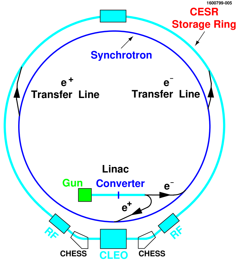
Figure 3.1: The CESR Accelerator Facility. The relevant components are the linac (located within the ring), synchrotron (located against the inner wall of the tunnel), and storage ring (located against the outer wall of the tunnel). The position of the tungsten target used for positron production is shown by the converter.

Electrons are generated by heating a filament until they have sufficient energy to escape from the filament surface. The electrons are then collected by a prebuncher which compresses the electrons into packets for acceleration in the linac. The accelerating sections of the linac have oscillating electric fields which are synchronized to increase the energy of the electrons as they travel through the components. The electrons are accelerated to an energy of about 300 MeV at the end of the linac.

Positrons are created by colliding an 140 MeV electron beam halfway down the linac on a movable tungsten target. The collisions create showers of positrons, electrons, and photons. The positrons are separated from the electrons and accelerated in the rest of the linac to an energy of about 200 MeV.

Bunches of electrons and positrons from the linac are separately fed into the synchrotron. The synchrotron consists of a series of dipole bending magnets and four 3-meter long linear accelerators. As the energy of the particles is increased by the linear accelerators in the synchrotron, the magnetic fields in the dipoles are also increased to keep the particles enclosed in the synchrotron. Once the particles are accelerated to the desired energy of $\sim$2 GeV, they are transferred to the storage ring.

The electrons and positrons are steered around the storage ring by a series of dipole bending magnets and focused by a series of quadrupole and sextupole magnets. There are also final-focusing quadrupole magnets located directly outside of the
CLEO-c detector. As the beams go around the storage ring, they lose energy by synchrotron radiation. The energy is replaced through the use of superconducting radio frequency (RF) cavities which operate at a frequency of 500 MHz.

The electrons and positrons in the storage ring travel around in a single 90 mm $\times$ 50 mm elliptical vacuum pipe with its major axis in the horizontal plane. In optimal running conditions, electrons and positrons are separately grouped into nine bunches called trains. Each train contains up to five bunches, with each train separated with a 14 ns spacing. Electron-positron collisions at non-desirable locations are prevented by four electrostatic separators with electric fields in the horizontal plane. These separators push the orbit of the electron and positron trains around each other into so-called pretzel orbits. Another interaction point potentially exists at the opposite side of the storage ring from the CLEO-c detector, but the beams are separated by two vertical electrostatic separators. At the interaction point enclosed by the CLEO-c detector, the beams do not collide head-on but with a small crossing angle of 2.5 mrad ($\approx 1/7~{}^{\circ}$) into the ring. This allows for bunch-by-bunch collisions of the electron and positron trains.

The CESR facility operated efficiently at nominal beam energies of $\sim$5.3 GeV from 1979 to 2003 for the production of the $\Upsilon(4S)$ resonance. The change of beam energy to $\sim$2 GeV required changes in CESR since the amount of energy emitted through synchrotron radiation, which is proportional to $E^{4}$ [163] ($E$ is the beam energy), decreases. Two important beam parameters are affected by the decreased amount of synchrotron radiation. The first parameter is the damping time of the betatron amplitude, which is related to the mean value of the transverse momentum of the beam. At the lower beam energies, the damping time, which is proportional to $E^{-3}$ [163], increases. The other parameter is the horizontal beam size. The total beam size of a particle bunch can be described as a six-dimensional phase space envelope (three in position space and three in momentum space) [165]. At lower beam energies, the horizontal beam size, which is proportional to $E^{2}$ [163], decreases, thereby restricting the particle density per bunch. These effects decrease the amount of attainable luminosity. It can be improved with the insertion of wiggler magnets into CESR.

A wiggler magnet, sometimes called a Siberian snake, consists of an even number of dipole magnets with high magnetic field intensities. The direction of the magnetic fields alternates between the successive magnetic elements of the wiggler. The magnetic field configuration shakes the beams in the horizontal plane, thereby increasing the amount of synchrotron radiation with minimal amounts of overall deviation in the beam path around the ring. The emission of the radiation decreases both the mean transverse and longitudinal momenta of the beam particles while increasing the dispersion of the momentum components. The decrease of the mean transverse momentum decreases the damping time, while the increase of the dispersion of the transverse momentum increases the horizontal beam size. The mean longitudinal momentum ($E$) is increased in the RF cavities, while the dispersion of the longitudinal momentum ($\sigma_{E}$) is decreased.

Twelve wigglers have been installed into CESR for operation at lower beam energies (note that only six wigglers magnets had been installed in CESR when the data used in this dissertation were taken). Each wiggler consists of eight dipole magnets with maximum magnetic field strengths of 2.1 Tesla per magnet [163]. The wiggler magnets increase the beam size by a factor of 4-8 and decrease the damping time by an order of magnitude, as compared to a storage ring without wiggler magnets [164]. The beam energy resolution ($\sigma_{E}/E$) from the wiggler dominated storage ring is $\sigma_{E}/E$ = 8.6$\times 10^{-4}$, four times larger than without wigglers [164].

The beam energy is measured by determining the orbit length traveled by the beams in the storage ring. To first order, the energy is determined by the bending dipole magnets [166]

$$E_{0}=\frac{ec}{2\pi}\sum_{i}|B_{i}|~{}\Delta\theta_{i}~{}\rho_{i},$$ (3.1)

where $e$ is the charge of the electron, $c$ is the speed of light in a vacuum. The variables $|B_{i}|$, $\Delta\theta_{i}$, and $\rho_{i}$ are the magnetic field strength, bending angle, and radius of curvature of the $i$th dipole magnet. The sum in Eqn. 3.1 is over all of the dipole magnets in the ring. Additional corrections to the beam energy are caused by the RF cavities, electrostatic separators, sextupole and wiggler magnets, and the different types, horizontal steering, and hysteresis of the dipole magnets. As an example of the uncertainty in the absolute value of the beam energy, Figure 3.2 shows the run-by-run hadronic cross section of the $\psi(2S)$ data sample, collected with the CLEO-c detector in December 2003 with CESR in the six wiggler configuration, as a function of nominal beam energy. Also shown in Figure 3.2 is the result of a numerical calculation program [167] which convolutes a non-relativistic Breit-Wigner with its mean centered at the $\psi(2S)$ mass ($M(\psi(2S))$ = 3686.093 $\pm$ 0.034 MeV, $\Gamma(\psi(2S))$ = 281 $\pm$ 17 eV [2]), the Gaussian beam energy resolution, and a Kureav-Fadin radiative tail [168]. Figure 3.2 shows that the beam energy is $\sim$0.7 MeV larger than expected. This leads to an absolute uncertainty in the center-of-mass energy of the $e^{+}e^{-}$ collision on the order of 1 MeV.

Figure 3.2: Run-by-run hadronic cross section of the CLEO-c $\psi(2S)$ data sample as a function of nominal beam energy. The points are individual data runs and the histogram is the result of a numerical calculation program which convolutes a non-relativistic Breit-Wigner for the $\psi(2S)$ resonance, the Gaussian beam energy resolution, and a Kureav-Fadin radiative tail. The observed cross section for the group of runs near $E_{beam}$ = 1.8438 GeV indicates that the $\psi(2S)$ peak occurs at a nominal energy which is $\sim$0.7 MeV higher than 1.8431 GeV corresponding to the known mass of $\psi(2S)$.

3.2 The CLEO-c Detector

The electron and positron beams are focused to collide at a point near the midpoint of the CLEO-c detector. Independent of the intermediate states, the final result of these collisions produces relatively long-lived charged and neutral particles. There are five different types of detected charged particles (and their corresponding antiparticles): the electron (denoted by e), muon ($\mu$), pion ($\pi$), kaon (K), and proton (p). The most common and easiest neutral particle to detect is the photon, while other neutral particles are either very difficult (the long lived neutral kaon $K^{0}_{L}$ and antineutrons) or nearly impossible (neutrons and neutrinos) to observe. The rest of this chapter is devoted to describing how we measure the properties of particles observed with the CLEO-c detector.

The CLEO-c detector is a cylindrically symmetric detector with its axis of symmetry aligned along the beam axis. It covers 93$\%$ of solid angle and is thus almost completely hermetic. The main components of the CLEO-c detector are the inner drift chamber [163], the main drift chamber [163, 169], the Ring Imaging Cherenkov (RICH) detector [163, 170, 171], the crystal calorimeter [163, 172], and the muon detection chamber [163, 172, 173]. All of the components, with the exception of the muon detector, are operated within a superconducting solenoidal coil which produces a uniform 1.0 Tesla magnetic field parallel to the axis of symmetry of the detector. The detector is schematically shown in Figures 3.3 and 3.4, and its components are described in the following sections. The chapter concludes with a discussion of the trigger and data acquisition systems.

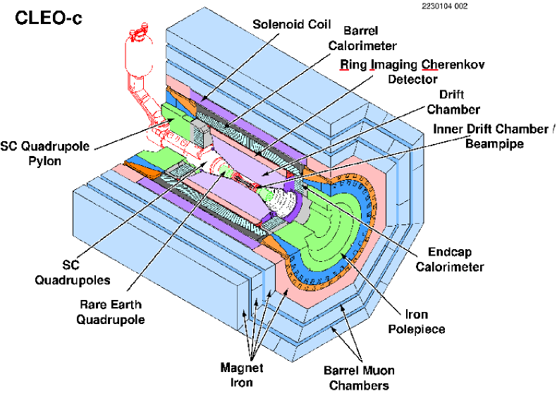
Figure 3.3: The CLEO-c detector. The outer and endcap layers of the muon detection chamber are omitted.

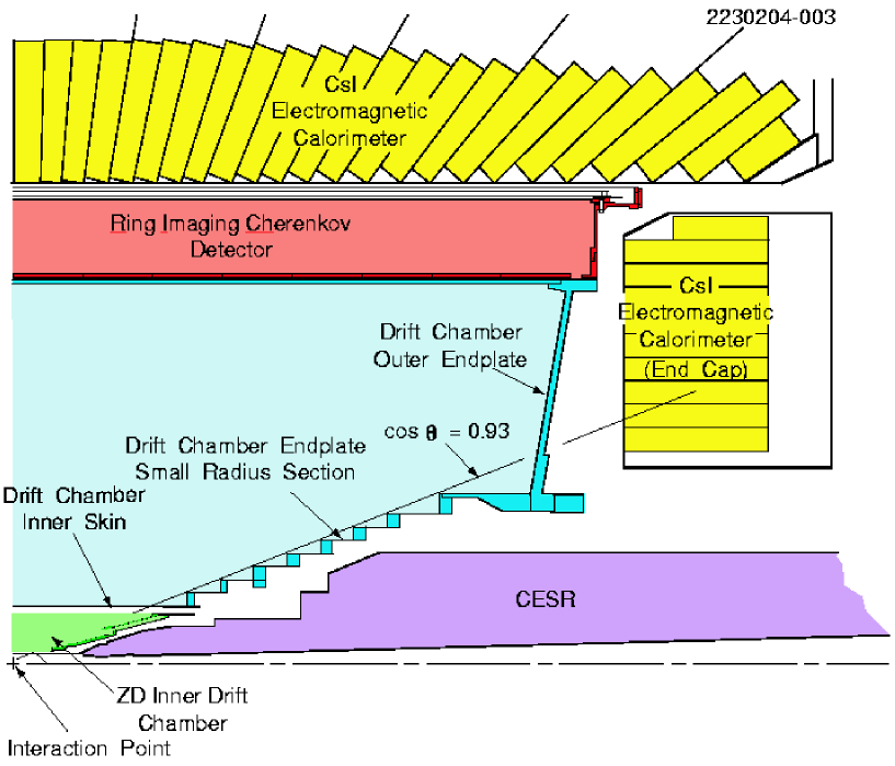
Figure 3.4: Cross section of the CLEO-c detector in the r-z plane.

3.2.1 The Inner Drift Chamber

Located immediately outside of the interaction point and beryllium beam pipe (radius of 3.5 cm, 0.5 mm thick) is the six-layer inner drift chamber. It can detect charged particles with $|$cos$\theta|$ $<$ 0.93, where $\theta$ is the angle between the particle and the positron beam, and consists of 300 drift cells filled with a helium-propane gas mixture. Each cell consists of a sense wire surrounded by eight field wires, forming a nearly square cell shape with a half cell size of 5 mm. The field wires are shared between neighboring cells, and neighboring layers are shifted laterally by one half cell width. A potential difference of 1900 V is applied to create an electric field between the sense and field wires. A charged particle ionizes the gas when it passes through a cell. The ionized electrons are then attracted toward the sense wire. The electric field near the sense wire is strong enough to cause the ionized electrons to ionize more atoms, which in turn creates an avalanche of electrons on the sense wire. The transit time of this electron pulse, synchronized with the timing structure of the electron and positron bunches in the storage ring, is converted into a distance of closest approach to the sense wire based on the drift velocity of the ionized electrons. The collection of ionized electrons on the sense wire constitutes a wire hit and is used in determining the trajectory of the charged particle.

The inner drift chamber covers a radial distance from 4.1 to 11.7 cm. The inner radial wall is made of 1 mm thick aluminum. The endplates are 16.5 cm machined aluminum plates located beyond the 93$\%$ solid angle coverage. The outer radial wall is made of 127 $\mu$m thick Mylar. The helium-propane gas mixture, with a radiation length of $\approx$ 330 m, and inner and outer walls constitute a radiation length of 1.2$\%$. The sense and field wires are made of 20 $\mu$m diameter gold-plated tungsten and 110 $\mu$m diameter aluminum wires, respectively. The wires in each layer are rotated in the $\phi$ direction to determine $z$ information of the charged particle. This rotation creates a so-called stereo angle, with the innermost layer being 10.5⁰ and the outermost layer being 15.4⁰ (stereo angle is defined as the $\phi$ difference that a wire makes between the endplate and the longitudinal center of the detector). This detector geometry provides a 680 $\mu$m resolution in the position of the charged particle creation along the beam axis ($z_{0}$). The inner drift chamber has a momentum resolution of $\sim$0.4$\%$ for charged particles at normal incidence (cos$\theta$ = 0) and is the only source of $z$ information for a charged particle with transverse momentum $<$ 67 MeV/$c$.

3.2.2 The Main Drift Chamber

Immediately outside of the inner drift chamber is the main drift chamber. It covers the radial distance from 13.2 to 82.0 cm and is the primary source of position and momentum measurements of charged particles. The main drift chamber consists of 9795 drift cells. The cells are arranged in 47 layers, with the first 16 layers having their field and sense wires aligned along the beam axis; the remaining 31 outer layers are rotated in a fashion similar to the inner drift chamber. The 31 stereo layers are combined into 4-layer “superlayers” which have alternating stereo angles of about 3⁰. The wire material, gas mixture, cell geometry, endplate material, power supplies, and readout electrons are the same as the inner drift chamber, with the exceptions that the half cell size is 7 mm and a potential difference of 2100 V is applied in each cell. The inner wall of the main drift chamber is 2.0 mm thick expanded acrylic with 20 $\mu$m aluminum skins. The outer radial wall, made of two layers of 0.8 mm thick aluminum cylindrical shells, is lined with 1 cm wide cathode pads. The cathodes provide a longitudinal position measurement at the outer radius and cover 78$\%$ of solid angle. The cathodes, when used with the stereo layers, improve the spatial measurement in the $z$ direction. Using a sample of $e^{+}e^{-}\rightarrow e^{+}e^{-}$ data events, it was shown that the resolution in the $z$ direction was improved from 1.5 mm to 1.2 mm with the inclusion of information from the cathodes [169]. The total radiation length of the main drift chamber is $\sim$2$\%$.

The energy loss of a charged particle due to ionization in the main drift chamber can be used for particle identification. The amount of energy loss per unit length ($dE/dx$) is related to the velocity of the particle. The $\chi^{2}$-like variable for particle identification relates the measured $dE/dx$ to the expected $dE/dx$ for particle hypothesis $i$ ($i$ = e,$\mu$,$\pi$,K, or p) by

$$S_{i}=\frac{(dE/dx)_{measured}-(dE/dx)_{expected,i}}{\sigma},$$ (3.2)

where $\sigma$ is the uncertainty in the $dE/dx$ measurement. Typical $dE/dx$ resolutions are around 6$\%$. Figure 3.5 shows measured $dE/dx$ as a function of momentum. It shows that kaons can be well separated from pions with momenta $\lesssim$ 500 MeV/$c$ and protons can be well separated from pions and kaons with momenta $\lesssim$ 1 GeV/$c$.

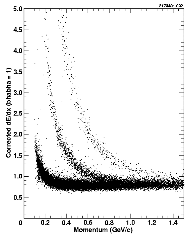
Figure 3.5: Measurement of $dE/dx$ as a function of particle momentum. The bands show the $dE/dx$ deposited by (from left to right) $\pi$, $K$, and protons, respectively.

The Kalman fitter procedure [174, 175] is used to reconstruct the path of the charged particle through the beam pipe, inner drift chamber, and main drift chamber. A charged particle moving in a vacuum through a solenoidal magnetic field traces out a helix, from which the momentum and position of the charged particle can be determined. The helix track needs to be corrected for various distortions caused by the material that the charged particle traverses. These distortions are mainly due to ionization energy loss and multiple scattering. Additional corrections include finite signal propagation time along the sense wires, flight time corrections of the ionized electrons in the drift cell, and the non-uniform magnetic field near the endcaps due to the final-focusing quadrupole magnets. Wire hits from both the inner and main drift chamber are used to reconstruct the trajectory of the particle. The momentum resolution is a function of the spatial resolution of individual hits, which is on average 88 $\mu$m. The momentum resolution for charged particles with 1 GeV/$c$ momenta at normal incidence is $\sim$0.6$\%$. The resolution is worse for charged particles with transverse momenta $<$ 120 MeV/$c$ because they will not transverse all 47 cell layers and the outer radius cathodes of the main drift chamber.

3.2.3 The RICH Detector

Outside of the main drift chamber is the Ring Imaging Cherenkov (RICH) detector. If the velocity of a charged particle is greater than the speed of light in the medium, it emits radiation in the form of Cherenkov photons. The photons are distributed in a conic shape and the apex angle of the cone, called the Cherenkov angle $\Theta$, is related to the particle velocity by

$$\mathrm{cos}~{}\Theta=\frac{1}{\beta n},$$ (3.3)

where $\beta$ is the velocity of the particle in units of $c$ and $n$ is the index of refraction of the medium. Equation 3.3 can be rewritten in terms of the momentum and mass of the particle as

$$\mathrm{cos}~{}\Theta=\frac{1}{n}~{}\sqrt{1+\frac{m^{2}}{p^{2}}}.$$ (3.4)

Therefore, the particle can be identified by measuring the Cherenkov angle and its momentum.

The RICH detector is a “proximity focusing” Cherenkov detector, which means that the Cherenkov photons are not focused and the Cherenkov angle is determined by allowing the photons to propagate over a finite space. The detector is composed of the following elements: a radiator material where the charged particle radiates Cherenkov photons, an expansion volume, and photon detectors. The radiators are made of lithium fluoride (LiF) plates. The expansion volume is 16 cm long and filled with nitrogen gas. The photon detectors are highly segmented multiwire proportional chambers (MWPC) filled with a methane-triethylamine (TEA) gas behind 2 mm calcium fluoride (CaF₂) windows. The detector covers the radial distance from 82 and 101 cm, its radiators cover 83$\%$ of solid angle, and constitutes a total radiation length of about 12$\%$. Figure 3.6 shows a schematic diagram of a one-tenth view of the RICH detector in the $r-\phi$ plane and an example of a charged particle, with its associated Cherenkov photons, propagating through its volume.

The components of the RICH detector are optimized for Cherenkov photons with a wavelength of 150 nm, for maximum quantum efficiency of the methane-TEA mixture in the photon detector. The index of refraction of the LiF radiators is $n$ = 1.50 at 150 nm. The nitrogen gas in the expansion volume and the CaF₂ windows have a transparency of $>$ 99.5$\%$ and $>$ 80$\%$ [171], respectively.

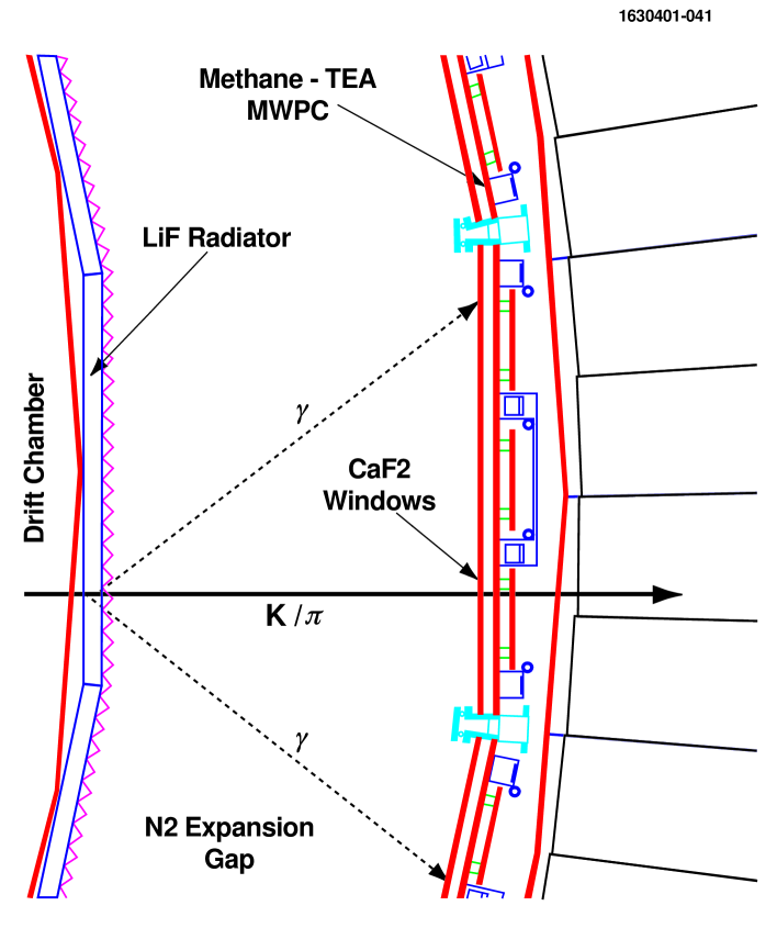
Figure 3.6: A one-tenth cross section view of the RICH detector in the $r-\phi$ plane. Also shown is the trajectory of a candidate charged track $K$ or $\pi$ and its associated Cherenkov photons.

The LiF radiators have a surface area of 17 cm $\times$ 17.5 cm and an average thickness of 1.0 cm. They are arranged in 14 coaxial rings with 30 radiators each. Emitted photons from charged particles at normal incidence would experience total internal reflection with flat surface radiators. The middle four rings, which accept particles with $|$cos$\theta|$ $\lesssim$ 0.4, have a “sawtooth” outer surface to overcome this problem and this radiator geometry is shown in Figure 3.6. Radiators at larger $|$cos$\theta|$ which do not have this problem have a flat planar outer surface.

The MWPC photon detectors are arranged to cover the same azimuthal angle as the radiators. The photoelectrons produced by a photon are detected by cathode pads, which have a surface area of 7.5 mm $\times$ 8.0 mm and are located 4.5 mm behind the CaF₂ windows. The cathode pads are arranged into 24 by 40 pad arrays with a total surface area of 30 cm $\times$ 19 cm. There are 8 arrays per MWPC, each separated by a 7 mm spacing. Axial anode field wires are placed 1 mm above the cathode pads with a spacing of 2.66 mm with 72 anode wires per MWPC. The anode wires are 20 $\mu$m diameter gold-plated tungsten with a 3$\%$ admixture of rhenium. The back plane of the CaF₂ windows has 100 $\mu$m wide silver traces spaced 2.5 mm apart. A 2700 V potential is applied between the silver traces and the anode wires. Examples of Cherenkov rings produced in sawtooth and flat radiators are shown in Figure 3.7.

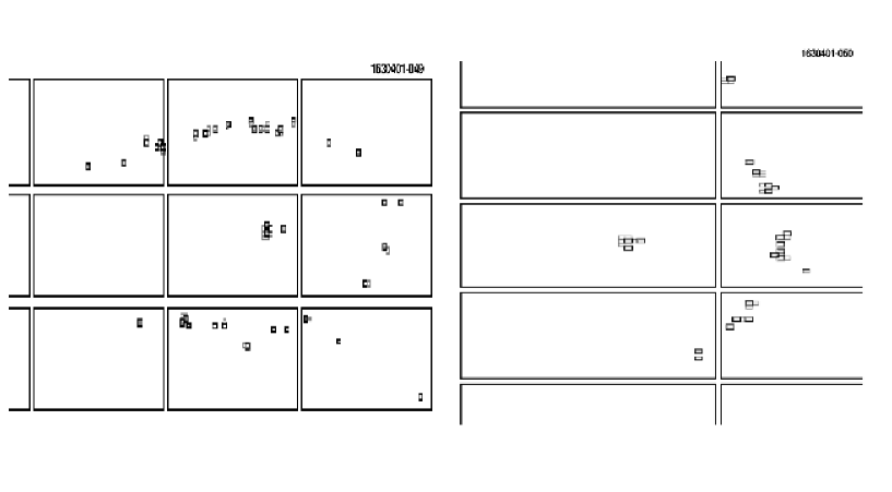
Figure 3.7: Cherenkov rings produced by a track transversing the sawtooth (left) and flat (right) radiators. The small rectangles are individual cathode pad hits and the large rectangles are the 24 $\times$ 40 cathode cell arrays. Only half of the Cherenkov ring is observed from flat radiators (right) because the other half experiences total internal reflection in the radiator; the ring shape from sawtooth radiators (left) is distorted due to the radiator surface geometry. The cathode hits near the center of the Cherenkov rings are from the incident charged particle crossing the cathode plane.

Precise measurement of the momentum vector of the charged particle at the radiator is important for the angular resolution of the Cherenkov cone. The main drift chamber has very good transverse momentum resolution but has larger uncertainty in the $z$ direction. The $z$ momentum component can be improved by as much as 50$\%$ if the charged particle can be associated with hits in the cathodes. The photons are traced out from their emitted point to the MWPC while also considering materials that it traverses along its path. The average number of observed photons for candidate particles is typically 12 and 10 photons from sawtooth and flat radiators, respectively. The angular resolution of a single photon produced in the sawtooth and flat radiators are $\sigma_{\theta}$ = 13.2 and 15.1 mrad, respectively. The angular resolution per track is determined by accepting all photons which are within $\pm$3$\sigma$ of the expected Cherenkov angle and weighting each photon by 1/$\sigma^{2}_{\theta}$; $\sigma_{\theta}$ = 3.7 and 4.9 mrad for sawtooth and flat radiators, respectively. Possible sources of uncertainties in the angular resolutions are from the location of the photon emission point, chromatic dispersion, position error of reconstructed photons, and trajectory of the charged track in the radiator.

Information from the Cherenkov photons is used to derive a likelihood for a particular particle hypothesis. The likelihood weights each possible optical path traveled by a photon by considering the length of the radiation path and the refraction probabilities from inverse ray tracing. A $\chi^{2}$-like particle identification variable can be obtained by taking the difference of the logarithm of two different particle hypotheses, given explicitly as

$$\chi^{2}_{i}-\chi^{2}_{j}=-2\mathrm{ln}L_{i}+2\mathrm{ln}L_{j},$$ (3.5)

where $L_{i}$ and $L_{j}$ denote the likelihood for particle hypotheses $i$ and $j$, respectively. Figure 3.8 shows an example for the kaon efficiency and pion fake rate as a function of different values of $\chi^{2}_{K}-\chi^{2}_{\pi}$ for momenta $>$ 0.7 GeV/$c$. The kaon efficiency is 92$\%$ and the pion fake rate is 8$\%$ when requiring a given particle to be more like a kaon than a pion, defined as $\chi^{2}_{K}-\chi^{2}_{\pi}$ $<$ 0. Figure 3.9 shows the particle separation as function of momentum when both particles are above their respective Cherenkov radiation thresholds.

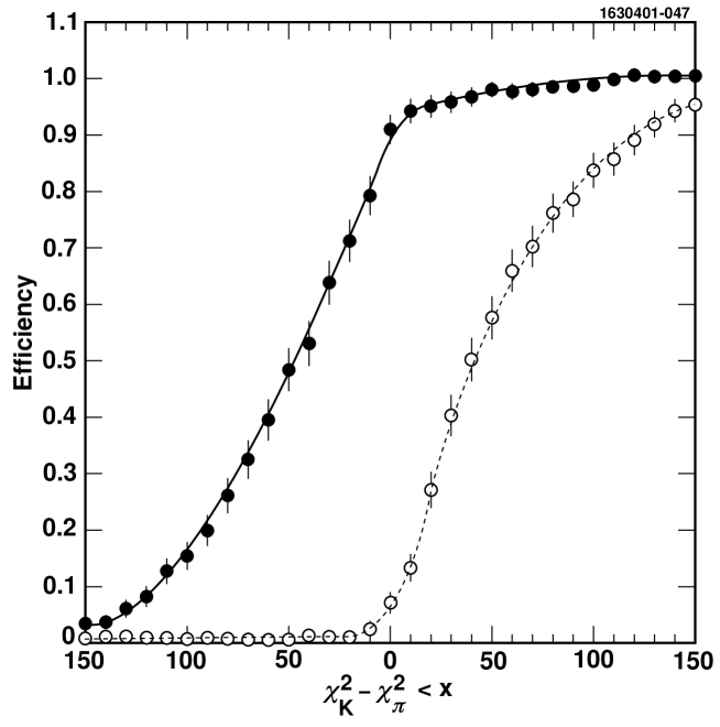
Figure 3.8: Kaon efficiency (solid points) and pion fake rate (open circles) determined from the RICH detector for various cuts on $\chi^{2}_{K}-\chi^{2}_{\pi}$ for kaons and pions with momenta $>$ 0.7 GeV/$c$.

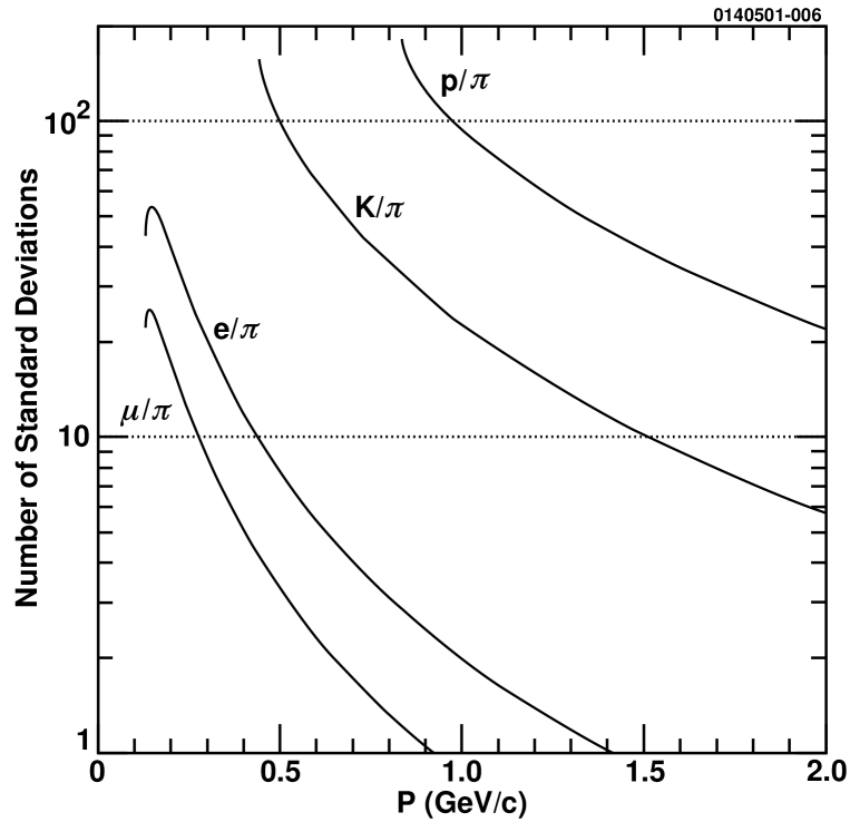
Figure 3.9: Particle separation in the RICH detector. The quantity plotted is $|\theta_{X}(P)-\theta_{\pi}(P)/\sigma(P)$ versus particle momentum for $X=e,\mu,K,$ or $p$, where $\sigma(P)=\sigma^{\beta=1}\sqrt{N^{\beta=1}_{\gamma}/N_{\gamma}(P)}$ is the rms resolution.

3.2.4 The Crystal Calorimeter

Located directly outside of the RICH detector in the radial direction and outside of the endcap of the main drift chamber is the electromagnetic calorimeter. The calorimeter consists of 7784 thallium-doped cesium iodide blocks. Three different types of reactions can occur in the crystals depending on the incident particle [176]. The first type of reaction is the production of an electromagnetic shower produced by incident photons, electrons, and positrons. Photons produce electron-positron pairs, while electrons and positrons emit bremstrahlung radiation. The bremstrahlung photons then produce electron-positron pairs. This produces a large number of low energy electrons, positrons, and photons. The low energy positrons and electrons annihilate to produce pairs of photons, and low energy photons begin to ionize the atoms. The low energy electrons are captured by thallium atoms in the crystal. The deexcitation of thallium emits visible light ($\lambda$ = 560 nm for CsI(Tl) [176]), which in turn is detected by a silicon photodiode. In the second type of reaction, the charged particle directly ionizes atoms in the crystal. The liberated electrons are captured by thallium atoms. This type of reaction occurs for all charged particles (with the exception of electrons and positrons). The last type of reaction occurs when hadrons interact strongly with an atomic nucleus in the crystal. These strong interactions can produce a large number of neutral pions, which decay to pairs of photons and produce electromagnetic showers.

The calorimeter is configured in three sections, a barrel region and two endcap regions, as shown in Figure 3.4. The barrel region accept particles in the $|$cos$\theta|$ range of $<$ 0.8, and the endcaps accept 0.85 $<|$cos$\theta|<$ 0.93. The transition region, defined by 0.8 $<$ $|$cos$\theta|$ $<$ 0.85, is generally not used, because detector material blocks the interaction point and there are shower spillovers between the barrel and the endcap. The barrel region covers a radial distance from 102.4 to 142.5 cm and has a length of 3.37 meters. It contains 6144 blocks arranged in 48 azimuthal rows with 128 blocks per row. The front surface of each block is aligned to point back to the interaction point, with a minor correction caused by the gaps between blocks pointing a few centimeters away to prevent incident particles from passing between adjacent blocks. The endcap sections contain 820 blocks and are four-fold symmetric in $\phi$. The front surfaces form a plane which is located 124.8 cm away from the interaction point. Each crystal block has a front surface area of 5 cm $\times$ 5 cm and a length of 30 cm, or 16 radiation lengths. Each block is wrapped with three layers of 0.04 mm white teflon and one layer of 0.01 mm aluminized mylar to ensure high internal reflection.

The light yield from a block is converted into electrical signals by four photodiodes attached to the back plane of each block; each with an active area of 1 cm $\times$ 1 cm. Each photodiode is connected to a separate nearby preamplifier. The four photodiodes for a given block are then summed by a mixer/shaper card. The output from the mixer/shaper card sends a signal to an analog-to-digital converter (ADC) and is also combined with other nearby blocks in a trigger tile to be used by the calorimeter trigger, described in more detail in the trigger section, Section 3.2.6.

The ADC values are converted into energies before shower reconstruction begins. This requires electronic pedestal subtraction, gain multiplication, and conversion to absolute energy units. Crystal-by-crystal energy calibrations are calculated using $e^{+}e^{-}\rightarrow e^{+}e^{-}$ (Bhabha) data events.

Energy from neighboring blocks are combined to determine the total shower energy from the incident particle, starting with the most energetic block if its energy exceeds 10 MeV. Varying the number of blocks included in determining the total energy of a shower as function of shower energy improves the shower energy resolution [172]. The number of blocks considered in a shower has a logarithmic dependence, ranging from 4 blocks at 25 MeV to 13 blocks at 2 GeV . The centroid of the shower is determined by an energy-weighted average of the block centers used in constructing the shower. The shower energy resolution in the barrel region is 4.0$\%$ at 100 MeV and 2.2$\%$ at 1 GeV. Figure 3.10 shows the shower energy resolution as a function of the number of summed blocks. The angular resolution for barrel showers is about 10 mrad. Showers reconstructed in the endcap regions are of comparable quality.

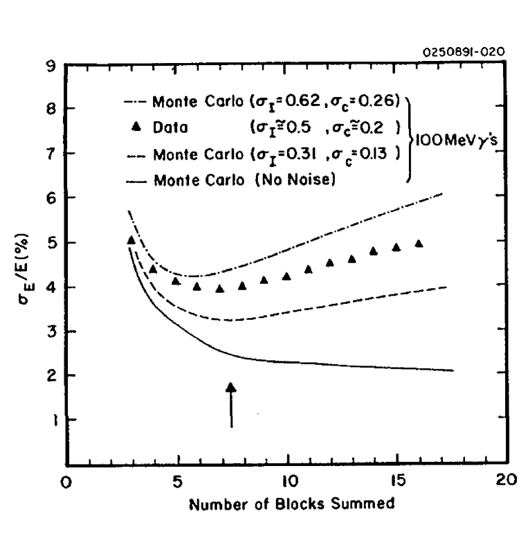
Figure 3.10: Shower energy resolution as a function of the number of summed blocks determined for the CLEO II detector. The calorimeter has remained unchanged since the installation of the CLEO II detector. The curves were generated from a Monte Carlo shower simulation of 100 MeV photons with appropriate noise included. The points were measured with experimental data from the 100 MeV photon lines from the transitions $\Upsilon(3S)\rightarrow\gamma\chi_{bJ}(2P)$. The arrow indicates the actual number of summed blocks for 100 MeV photons.

3.2.5 The Muon Detector

The muon detector, as shown in Figure 3.11, consists of a system of proportional chambers interspersed in the return iron of the solenoid magnet. The muon detector covers 85$\%$ of solid angle. In the barrel region, the chambers are located behind 36, 72, and 108 cm of iron at normal incidence and located at respective radial distances of 2.10, 2.46, and 2.82 meters. Chambers are also placed outside of the endcap iron at a distance of 2.82 meters away from the interaction point. The total available thickness of iron absorber varies from about 7.2 to 10.0 nuclear interaction lengths (n.l.) depending on their flight direction (1 n.l. = 16.7 cm of iron [2]).

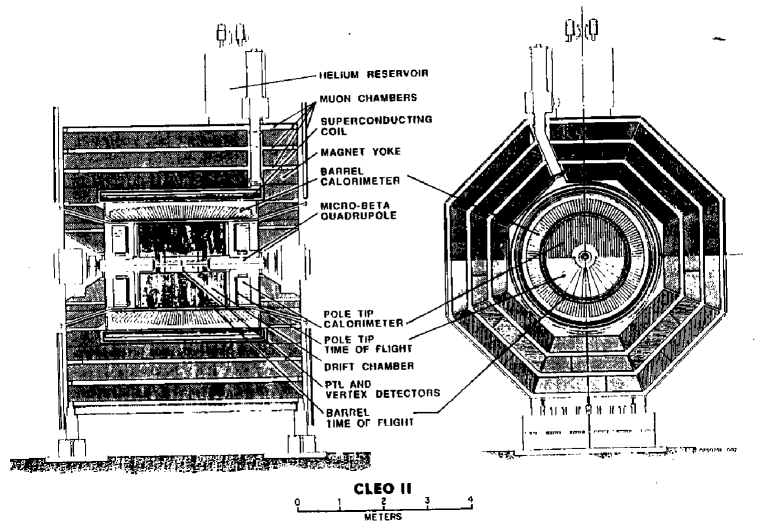
Figure 3.11: The CLEO II detector, showing the barrel and endcap muon chambers. The muon chambers has remained unchanged since the installation of the CLEO II detector.

A muon chamber, as shown in Figure 3.12, consists of three layers of proportional counters interspersed with copper pickup strips. The middle counter layer is offset by one half cell width to improve geometric acceptance. A proportional counter, as shown in Figure 3.13, is made of 5 m long, 8.3 cm wide PVC plastic. Each counter has eight 9 mm $\times$ 9 mm U-shaped rectangle cells, all enclosed in a 1 mm thick PVC sleeve. Each cell has a 50 $\mu$m diameter silver-plated copper-beryllium anode wire and is filled with an argon-ethane gas mixture. The three sides of a cell are coated with graphite providing the cathode for the cell. Each cell is operated in the proportional mode with a potential of 2500 V. For position measurements orthogonal to the counter length, 8.3 cm wide external copper pickup strips are located on top of each counter. In total, the muon detector consists of 2352 counters and 5472 strips.

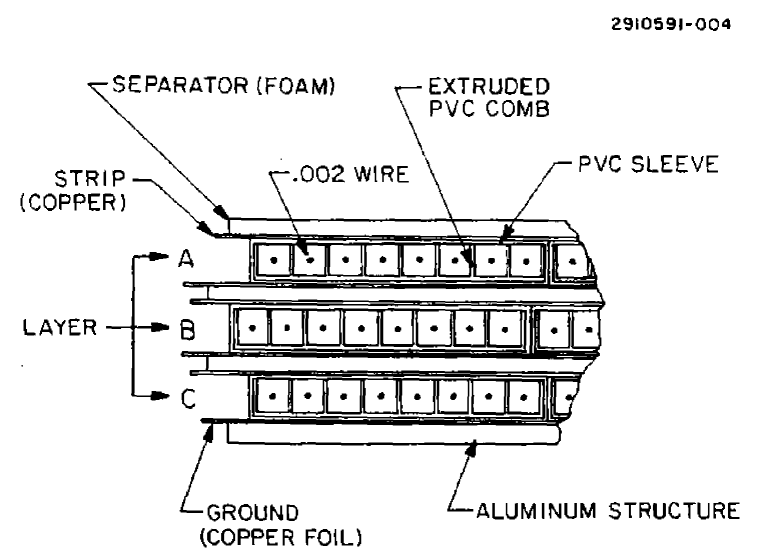
Figure 3.12: Cross section of a muon chamber. It consists of three layers of 8-cell proportional counters interspersed with copper pickup strips. The middle counter layer is offset by one half cell width to improve geometric acceptance.

Figure 3.13: Cross section of the proportional counter for the muon detector.

To determine if a hit in the muon detector is associated with a charged particle track, the track is traced out from the main drift chamber and, after taking into account multiple scattering and energy loss, it is projected through the muon detector. A two-dimensional $\chi^{2}$ fit is performed to test if the hit can be associated with the track. The hit in the muon chamber is identified with the track if $\chi^{2}$ $<$ 16. The resolution for anodes located in the three barrel chambers (increasing in distance from the interaction point) is 3.7, 4.6, and 5.7 cm, respectively; in the endcap chambers, the resolution is 7.2 cm. The corresponding resolution for the strips are 5.5, 7.0, 7.5, and 9.0 cm. Particles must have momenta in excess of 1.0 GeV/$c$ to be detected in the muon detector. In the momentum range 1.5-2.0 GeV/$c$, the efficiency for muons to penetrate $>$ 3, $>$ 5, and $>$ 7 n.l. is about 90$\%$, 85$\%$, and 30$\%$, respectively. The efficiency is also stable over the entire $|$cos$\theta|$ range except for a slightly lower efficiency at the largest $|$cos$\theta|$ (near the beampipe). The fake rate for pions and kaons to transverse 3 n.l. in the same momentum range is about 4$\%$ and 12$\%$, respectively.

3.2.6 The Trigger System

This description of the trigger is based on Refs. [163], [177], [178], and [179]. A schematic view of the trigger system [163] is shown in Figure 3.14. Data from the main drift chamber and crystal calorimeter are received and processed on separate VME crates by appropriate circuit boards to yield basic trigger primitives such as track count and topology in the main drift chamber and shower count and topology in the calorimeter. The information from both systems is correlated by global trigger circuitry which generates an ’pass’ strobe every time a valid trigger condition is satisfied. The ’pass’ signals are conditionally passed by the data flow control (DFC) circuitry to the gating and calibration (GCAL) modules for distribution to the data acquisition system. In addition, online luminosity information is determined by the luminosity (LUMI) module from calorimeter information and sends it to the CESR accelerator control room via the global trigger.

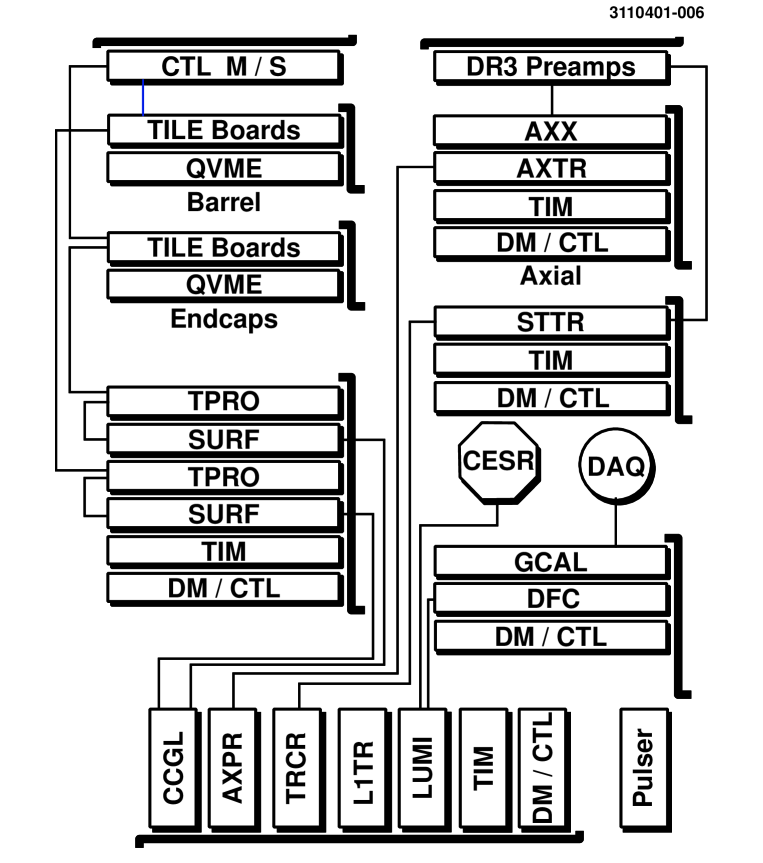
Figure 3.14: Overview of the trigger system. For the explanation of symbols, see text.

The trigger system consists of two tracking triggers [177], one using information from the axial layers of the main drift chamber and the other using the stereo layers, a calorimeter trigger [178], and a decision and gating global trigger system [179]. Configuration and supervision duties are provided by MVME2304 PowerPC modules, which play the dual role of crate controller (CTL) and data mover (DM). Also, for clock and ’pass’ signal distribution, as well as busy signaling, a trigger interface module (TIM) is used. The details of the tracking, calorimeter, and global triggers are discussed in the following subsections.

Tracking Triggers

The limited wire count in the axial portion of the main drift chamber makes it possible to build a tracker that examines the complete set of 1696 axial wires in the first 16 layers of the main drift chamber for possible valid patterns caused by tracks having transverse momenta $>$ 133 MeV/$c$. Patterns from tracks missing the central axis of the beam pipe by as much as 5 mm are included.

The axial trigger bins the data into 42 ns wide time slices, three times longer than the bunch spacing in a beam train. This discretization is sufficient for the time resolution required by the trigger, namely to determine the time of the interaction, with a fixed offset, to within 100 ns. Pattern recognition is performed by the axial tracking (AXTR) boards for the entire axial portion of the main drift chamber.

The axial processor (AXPR) takes the 112 $\phi$ tracking bits from the AXTR boards and produces a 7 bit track count, a 48 bit array which represents the azimuthal event topology, and a 2 bit time stamp. The information from the AXPR boards are then passed to the track correlator (TRCR) boards.

The stereo section of the main drift chamber (layers 17-47) differs from the axial section in that the stereo wires are offset with respect to the beam, or $z$, axis; the axial wires are almost exactly parallel. The stereo section is broken up into eight superlayers. The first seven superlayers have four layers of wires each; the last has only three. The odd superlayers are called the U superlayers and have a positive $\phi$ tilt with respect to the $z$-axis; the even ones are V superlayers and have a negative tilt.

There are too many (8100) wires in the stereo section of the main drift chamber for the stereo tracker to examine every wire individually. Instead, the stereo tracker receives 1 bit for every 4 by 4 block of wires. The U and V superlayers are tracked separately.

The stereo block definitions (which patterns within a 4 by 4 block are defined as track segments) and the stereo road definitions (which groups of U or V blocks is considered a valid track) were generated from simulated tracks having transverse momenta $>$ 167 MeV/$c$. In order to satisfy a stereo block pattern, a hit must be present on at least 3 out of 4 layers, allowing high track efficiency for realistic wire hit efficiencies. Stereo roads, however, do not allow from missing blocks.

One stereo tracking (STTR) board is responsible for one-sixth of the U or V superlayers (12 boards total for the stereo trigger). To prevent inefficiencies at board boundaries, information is shared between neighboring STTRs. As with the axial trigger, pattern recognition is performed every 42 ns. The outputs from each STTR are sent to the TRCR boards for further processing.

Topological information from both the axial and stereo tracking trigger hardware is received by two TRCR boards. The TRCRs correlate the U, V, and axial projection bits to form a final set of 48 correlated azimuthal projection bits as well as high and low momentum track counts. The derived TRCR output information is sent to the Level 1 decision electronics.

The stereo tracking trigger provides high efficiency per track and good background rejection. The combined axial plus stereo tracking trigger is much less sensitive to backgrounds than the axial trigger alone, while maintaining an efficiency of $>$ 99$\%$ for single tracks.

Calorimeter Trigger

The calorimeter trigger incorporates both analog and digital electronics to provide
pipelined trigger information every 42 ns with a latency of $\sim$2.5 $\mu$s. Analog processing is employed to address the quantization error caused by split energy deposition in adjacent calorimeter blocks, and digital field programmable gate arrays are used extensively to filter and categorize the calorimeter energy topology. Timing, position, and energy information are all available for use in the calorimeter trigger.

Complications associated with boundaries in the calorimeter are reduced by creating overlapping ’tiles’ by forming analog sums of signals from groups of 64 calorimeter blocks, as shown by the example in Figure 3.15. A photon striking the calorimeter will deposit nearly all of its energy in at least one of the groups of blocks summed in a tile. Naturally, a signal in a single block will appear in four different tiles; it is the task of the tile processors (TPRO) to account for this.

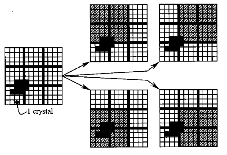
Figure 3.15: An example of calorimeter trigger tiles. A 12 by 12 block subregion of the calorimeter is shown, with a single crystal block represented by an individual box. An example of a photon shower is represented by the cluster of solid boxes, and trigger tiles are denoted by the area covered by dashed lines.

The TPRO boards receive data from as many as 384 active tiles in the calorimeter barrel and 120 tiles in the endcaps. The first task of the TPRO is to filter event data so that adjacent or overlapping tiles which contain energy are reduced to a single hit. After filtering the data, the TPRO then determines the number of showers and their position in the calorimeter. The algorithm run by the TPRO boards is a comprise between the angular and energy resolutions and the desire to limit the amount of information to be processed by the trigger. The TPROs remove all but the highest threshold tile in a group of adjacent or overlapping tiles and project the two-dimensional tile information into one-dimensional distributions in $\theta$ and $\phi$.

Once the individual TPROs have produced their results, one SURF (Sampling Unit for Radio Frequency) board combines the four barrel TPRO projections and tile counts. A second SURF board does the same for the endcap TPROs. The output from the SURF boards are sent to the crystal calorimeter global logic (CCGL) for use by the Level 1 decision electronics.

Global Trigger

The global decision and data flow control system produces and distributes a trigger decision every 42 ns based on input from the tracking and calorimeter triggers described above. Programmable trigger decision (L1TR) boards monitor this information. Tracking and calorimeter information is received and channeled through variable-depth pipelines to time-align the data; tracking is available in $\sim$2 $\mu$s while the calorimeter requires over 2.5 $\mu$s. The time-aligned information is presented on a shared backplane where several L1TR modules have access to the information for performing independent trigger condition evaluation.

All L1TR boards see the same input information on the Level-1 backplane. The trigger logic section allows the user to define 24 independent trigger “lines”, each a (potentially complex) combinatoric function of the 179 inputs. Each of the 24 trigger lines is routed through a 24 bit prescalar to a 40 bit scalar. In the present mode of operation we typically run with a set of about eight trigger lines. The definitions of these lines are shown in Table 3.1. Once the criteria for a trigger line is satisfied, the detector information is sent to the data acquisition system.

Table 3.1: Definitions of the trigger lines. Note that the random trigger only sends out one of 1000 Level 1 decisions to the data acquisition system, i.e., prescaled by 1000.

Name	Definition
Hadronic	$(N_{axial}>1)\&(N_{CB~{}low}>0)$
Muon Pair	Two back-to-back stereo tracks
Barrel Bhabha	Two back-to-back high showers in barrel
Endcap Bhabha	Two back-to-back high showers in endcaps
Electron track	$(N_{axial}>0)\&(N_{CB~{}med}>0)$
Tau	$(N_{stereo}>1)\&(N_{CB~{}low}>0)$
Two Track	$N_{axial}>1$
Random	random 1 kHz source

3.2.7 The Data Acquisition System

This description of the data acquisition system is based on Ref. [163]. The data acquisition (DAQ) system [163] consists of two equally important parts. The data collection system is responsible for the data transfer from the front-end electronics to the mass storage device, while the slow control system monitors the data quality and the detector components. A block diagram of the DAQ system for the CLEO III detector is shown in Figure 3.16. The only change between the CLEO III and CLEO-c detector, and the corresponding change in the DAQ system, is the replacement of the Silicon vertex detector (Si-VERTEX) with the inner drift chamber.

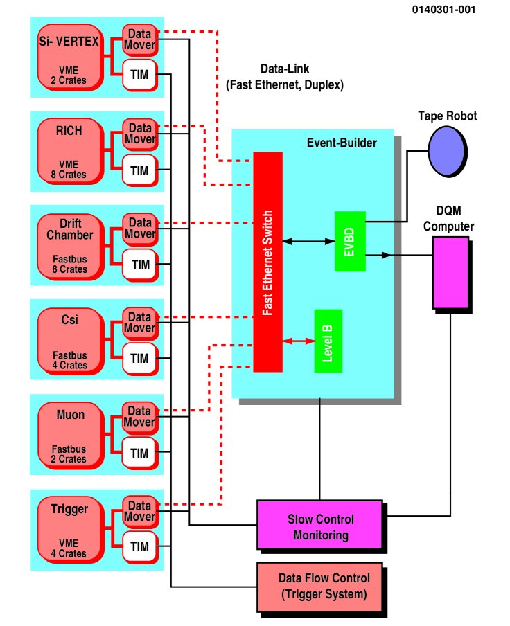
Figure 3.16: Block diagram of the CLEO III data acquisition system. The only change between the CLEO III and CLEO-c detector, and the corresponding change to the DAQ system, is the replacement of the Silicon vertex detector (Si-VERTEX) with the inner drift chamber.

For each event accepted by the trigger, approximately 400,000 detector channels have to be digitized. Front-end data conversion is performed in parallel and local buffers on each databoard hold the data for later asynchronous readout by the DAQ. Data sparsification is performed directly on the databoards. The Data Mover, a dedicated module in each front-end crate, assures transfer times below 500 $\mu$s and provides a second buffer layer. Using data links based on the Fast Ethernet protocol, the event fragments are transmitted from the crates to the Event Builder. Completely assembled events are transferred to mass storage and a fraction of the data is analyzed online by the CLEO monitor program (Pass1) to quickly discover problems and to ensure the quality of the data written to tape.

The flow of event data through the data collection system is controlled by a simple control protocol. The basic philosophy is to rearm the experiment to wait for the next trigger only when sufficient buffer space is available to receive a new event, i.e., a free slot at the databoard.

Independent from the main data path, a slow control system monitors the individual detector components. Run control as well as the initialization of the detector subsystems are also part of the slow control system.

The key parameters for the DAQ system are the trigger rate, the acceptable deadtime, as well as the average event size. These quantities constrain the readout and digitization time in the front-end electronics as well as the data transfer bandwidth the DAQ system has to provide. The performance parameters of the DAQ system are listed in Figure 3.2. The readout time is defined as the time between the trigger signal and the end of the digitization process in the front-end electronics. For each event accepted by the trigger, this causes deadtime, and hence it is desirable to keep the readout time as short as possible. The maximum readout induced detector deadtime is, on average, $<3\%$.

Table 3.2: Performance parameters of the DAQ system.

Name	Achieved Performance
Maximum Readout Rate	150 Hz (data taking)
	500 Hz (random test trigger)
Average Eventsize	25 kBytes
Average Readout Time	30 $\mu$s
Data Transfer Bandwidth	6 MBytes/s

Chapter 4 Analysis of Data

4.1 Data Sample

Table 4.1 lists the continuum and $\psi(2S)$ data samples used in the present analysis.

Table 4.1: Continuum and $\psi(2S)$ data samples.

Data sample	$\sqrt{s}$ (GeV)	$\cal{L}$ (pb-1)
Continuum	3.671	20.7
$\psi(2S)$	3.686	2.89

The luminosity for the continuum data sample is determined by comparing the QED processes $e^{+}e^{-}\rightarrow e^{+}e^{-}$, $e^{+}e^{-}\rightarrow\mu^{+}\mu^{-}$, and $e^{+}e^{-}\rightarrow\gamma\gamma$ to their respective calculated cross sections [181]. The calculated cross sections and the efficiencies for the respective QED final states are determined by the Babayaga generator [180], which include corrections for the initial state radiation and, for the $e^{+}e^{-}\rightarrow l^{+}l^{-}$ final states, interference from the J/$\psi$, $\psi(2S)$, and $\psi(3770)$ resonances. The luminosity for the $\psi(2S)$ data sample is determined from only the $e^{+}e^{-}\rightarrow e^{+}e^{-}$ and $e^{+}e^{-}\rightarrow\gamma\gamma$ processes due to contamination of the $\mu^{+}\mu^{-}$ final state from the $\psi(2S)\rightarrow\mu^{+}\mu^{-}$ decays [182]. The $\psi(2S)\rightarrow\mu^{+}\mu^{-}$ and $\psi(2S)\rightarrow e^{+}e^{-}$ decays in the $\psi(2S)$ sample account for $(43\pm 5)\%$ and $(2.7\pm 0.1)\%$ of the total $\mu^{+}\mu^{-}$ and $e^{+}e^{-}$ events observed, respectively. The errors in the above fractions arise from the current experimental uncertainties in the $\psi(2S)\rightarrow\mu^{+}\mu^{-}$ and $\psi(2S)\rightarrow e^{+}e^{-}$ branching ratios [2]. The total uncertainties in the luminosities are 1$\%$ [181] and 3$\%$ [182] for the continuum data sample and $\psi(2S)$ data samples, respectively.

The primary data sample for our form factor determinations is the continuum data sample. The $\psi(2S)$ data sample is used for two purposes: (i) it allows the opportunity to test and tune the selection criteria on an independent data sample by measuring the $\psi(2S)$ branching ratios to the final states of interest, and (ii) since the continuum data is only 15 MeV below the $\psi(2S)$ resonance, it allows us to take account of the contribution of the tail of the $\psi(2S)$ resonance in the continuum data sample.

The number of the produced $\psi(2S)$ in the $\psi(2S)$ data sample is determined from the number of observed hadronic events. The number of produced $\psi(2S)$ is $1.52\times 10^{6}$ with a systematic uncertainty of $3\%$ [183].

The continuum data sample needs to be corrected for the contamination from the tail of the $\psi(2S)$ resonance. A contamination scale factor is determined by using the number of observed $\pi^{+}\pi^{-}J/\psi$ events in the continuum and $\psi(2S)$ data samples [184]. The resulting scale factor is

$$C^{\pi^{+}\pi^{-}J/\psi}=\frac{N^{\pi^{+}\pi^{-}J/\psi}_{cont}}{N^{\pi^{+}\pi^{-}J/\psi}_{\psi(2S)}}=\frac{221\pm 15}{30518\pm 175}=0.0072\pm 0.0005$$ (4.1)

where $N^{\pi^{+}\pi^{-}J/\psi}_{cont}$ and $N^{\pi^{+}\pi^{-}J/\psi}_{\psi(2S)}$ are the number of observed $\pi^{+}\pi^{-}J/\psi$, $J/\psi\rightarrow l^{+}l^{-}$ events observed in the continuum and $\psi(2S)$ data samples, respectively. This scale factor is found to be in good agreement with the one determined from the luminosities and the evaluation of the $\psi(2S)$ tail [184].

4.2 Monte Carlo Samples

In order to determine the suitable criteria for event selection and background rejection for the $e^{+}e^{-}\rightarrow h\overline{h}$ ($h=\pi^{+},K^{+},p$) processes, Monte Carlo (MC) samples are generated for the following processes: $e^{+}e^{-}\rightarrow h\overline{h}$ (signal MC), $e^{+}e^{-}\rightarrow\gamma J/\psi,J/\psi\rightarrow h\overline{h}$ (ISR $J/\psi$ MC), and $e^{+}e^{-}\rightarrow l^{+}l^{-}$ (leptonic MC), where $l$ = $e,\mu$. The hadronic final state MC samples are generated with the EvtGen generator [185], while the leptonic MC samples are generated with the Babayaga generator [180]. All MC samples described above incorporate final state radiation emitted from the charged particles [186].

The $e^{+}e^{-}\rightarrow h\overline{h}$ MC samples are generated with proper angular distributions. The $e^{+}e^{-}\rightarrow\pi^{+}\pi^{-}$ and $e^{+}e^{-}\rightarrow K^{+}K^{-}$ MC samples are generated with a sin${}^{2}\theta$ angular distribution, where $\theta$ is the angle between the charged hadron and the positron beam, as defined in Eqn. 1.15. Two different sets of $e^{+}e^{-}\rightarrow p\overline{p}$ MC samples are generated based on different assumptions of the proton electric form factor. The two different assumptions are $|G^{P}_{E}(s)|$ = 0 and $|G^{P}_{E}(s)|$ = $|G^{P}_{M}(s)|$. The proton form factors are related to the differential cross section for their pair production at $\sqrt{s}$ as follows

$$\frac{d\sigma_{0}(s)}{d\Omega}=\frac{\alpha^{2}}{4s}\beta_{p}\left[|G^{P}_{M}(s)|^{2}~{}(1+\mathrm{cos}^{2}\theta)+\left(\frac{4m^{2}_{p}}{s}\right)|G^{P}_{E}(s)|^{2}~{}(\mathrm{sin}^{2}\theta)\right].$$

$$=\frac{\alpha^{2}}{4s}\beta_{p}|G^{P}_{M}(s)|^{2}(1+\eta)\left[1+\left(\frac{1-\eta}{1+\eta}\right)\mathrm{cos}^{2}\theta\right],$$ (4.2)

where $\alpha$ is the fine-structure constant, $m_{p}$ is the proton mass, $\beta_{p}$ is the proton velocity (in terms of c) in the laboratory system, $|G^{P}_{M}(s)|$ and $|G^{P}_{E}(s)|$ are the magnetic and electric form factor of the proton, respectively, and

$$\eta=\frac{4m^{2}_{p}}{s}\frac{|G^{P}_{E}(s)|^{2}}{|G^{P}_{M}(s)|^{2}}.$$ (4.3)

At $\sqrt{s}$ = 3.671 GeV, the angular distributions are 1 + cos${}^{2}\theta$ for $|G^{P}_{E}(s)|$ = 0 and
1 + (0.59)cos${}^{2}\theta$ for $|G^{P}_{E}(s)|$ = $|G^{P}_{M}(s)|$.

The hadronic final state MC samples consist of 20,000 generated events. Each sample uses the same 10 continuum data run numbers, which allows for a sampling of realistic detector effects.

The leptonic MC samples simulate the number of dilepton events in the continuum data sample. The cross sections listed below are determined by the Babayaga generator [180]. The cross section for Bhabha events ($e^{+}e^{-}\rightarrow e^{+}e^{-}$) at $\sqrt{s}$ = 3.671 GeV and each track having $|$cos$\theta|$ $<$ 0.8 is $\sigma_{Bhabha}$ = 126.50 $\pm$ 0.14 nb. With a total integrated luminosity of $\cal{L}$ = 20.4 pb^-1, a sample of 2.59$\times$10⁶ Bhabha events is generated. The cross section for dimuon events ($e^{+}e^{-}\rightarrow\mu^{+}\mu^{-}$) at $\sqrt{s}$ = 3.671 GeV, with the same track $|$cos$\theta|$ requirement, is $\sigma_{dimuon}$ = 4.999 $\pm$ 0.015 nb. This corresponds to a sample of 102,500 dimuon events. The leptonic MC samples are generated using all of the continuum data run numbers, and the number of events in each run is weighted according to its luminosity.

In order to study other possible background sources, a generic sample of $\psi(2S)$ MC decays is analyzed. The sample consists of 40,568,651 events or 26.7$\times$ the
CLEO-c $\psi(2S)$ data sample. The $\psi(2S)\rightarrow h\overline{h}$ branching ratios from the generic $\psi(2S)$ MC sample are not determined because the angular distributions of the $\psi(2S)\rightarrow h\overline{h}$ decays are thrown according to phase space and no final state radiation is incorporated.

4.3 Particle Identification Definitions

In order to discriminate between the $e$, $\mu$, $\pi$, $K$, and $p$ charged particles, particle identification (PID) information from the specific ionization ($dE/dx$) measured in the main drift chamber and Cherenkov radiation information from the RICH detector are used to form a joint $\chi^{2}$ function. For $dE/dx$, we form a quantity $S_{i}$ ($i=e,\mu,\pi,K,p$), which is

$$S_{i}=\frac{(dE/dx)_{meas}-(dE/dx)_{expected,i}}{\sigma}.$$ (4.4)

The measured $dE/dx$ of the charged track is $(dE/dx)_{meas}$, the expected $dE/dx$ for particle hypothesis $i$ is $(dE/dx)_{expected,i}$, and the uncertainty in the $dE/dx$ measurement is $\sigma$. The information from the RICH detector is given in the form of a likelihood function, $-2{\rm log}L$. The joint $\chi^{2}$ function is

$$\Delta\chi^{2}(i-j)=-2{\rm log}L_{i}+2{\rm log}L_{j}+S_{i}^{2}-S_{j}^{2}.$$ (4.5)

The more negative $\Delta\chi^{2}$, the higher the likelihood the particle is of type $i$ compared to type $j$.

Information from the crystal calorimeter (CC) and the main drift chamber is also used for charged particle identification. A CC shower is “matched” to a charged particle track if the shower is within 8 cm transverse to the position vector of the track at the front of the CC surface and 15 cm along the direction of the vector of the track. The CC energy associated with a track, denoted by $E_{tkCC}$, is the sum of all CC crystal energies in the shower associated with the track. The ratio $E_{tkCC}/p$ is also used and is defined as the ratio of the CC shower energy associated with the track to the momentum of the track measured with the inner and main drift chambers.

4.4 Kinematics of Two Track Events

Figures 4.1, 4.2, and 4.3 show the MC distributions for direct production of the two track final states which satisfy the acceptance, trigger, and tracking criteria. The variable $X_{h}$ is the total energy of the two tracks, assuming the particle hypothesis of interest for each track, normalized to $\sqrt{s}$. The signal regions are defined as 0.98 $<$ $X_{h}$ $<$ 1.02. An event passes the acceptance criteria when it has

• Number of tracks ($N_{trk}$) = 2

• Net charge ($\Sigma Q$) = 0

• Each track with $|$cos$\theta$$|$ $<$ 0.8

The trigger criteria are given in Table 3.1. A track passes the tracking criteria when it has

• $|d_{b}|$ $<$ 5 mm, and $|z_{b}|$ $<$ 5 cm (IP)

• 0.5 $<$ DRHF $<$ 1.2, and $\chi^{2}/dof$ $<$ 10 (Track Quality).

The interaction point (IP) variables $d_{b}$ and $z_{b}$ are the distances between the origin of the helix fit and the position of the $e^{+}e^{-}$ annihilation in the plane perpendicular to and along the axis defined by the positron beam, respectively. DRHF is defined as the number of inner and main drift chamber wire “hits” observed vs. the number of “hits” expected from the helix fit. The reduced $\chi^{2}/dof$ is the fit confidence normalized by the number of degrees of freedom of the track helix fix.

Figure 4.1: MC $X_{\pi}$ distributions with the acceptance, trigger, and tracking criteria applied. The distributions are from $e^{+}e^{-}\rightarrow\pi^{+}\pi^{-}$ signal MC (solid histogram at $X_{\pi}$ = 1), $e^{+}e^{-}\rightarrow K^{+}K^{-}$ signal MC (dot-dashed), $e^{+}e^{-}\rightarrow p\overline{p}$ signal MC obtained with $|G^{P}_{E}(s)|$ = 0 (solid at $X_{\pi}$ = 0.87), Bhabha MC (dashed), and dimuon MC (dotted). The hadronic distributions ($\pi^{+}\pi^{-}$, $K^{+}K^{-}$, $p\overline{p}$) are arbitrary normalized while the dileptonic distributions ($e^{+}e^{-}$, $\mu^{+}\mu^{-}$) correspond to the number of leptonic events at $\sqrt{s}$ = 3.671 GeV and a 20.4 pb^-1 data sample. The signal region is defined as 0.98 $<$ $X_{\pi}$ $<$ 1.02 and is enclosed between the vertical lines.

Figure 4.2: MC $X_{K}$ distributions with the acceptance, trigger, and tracking criteria applied. The distributions are from $e^{+}e^{-}\rightarrow\pi^{+}\pi^{-}$ signal MC (dot-dashed), $e^{+}e^{-}\rightarrow K^{+}K^{-}$ signal MC (solid histogram at $X_{K}$ = 1), $e^{+}e^{-}\rightarrow p\overline{p}$ signal MC obtained with $|G^{P}_{E}(s)|$ = 0 (solid at $X_{K}$ = 0.90), Bhabha MC (dashed), and dimuon MC (dotted). The hadronic distributions ($\pi^{+}\pi^{-}$, $K^{+}K^{-}$, $p\overline{p}$) are arbitrary normalized while the dileptonic distributions ($e^{+}e^{-}$, $\mu^{+}\mu^{-}$) correspond to the number of leptonic events at $\sqrt{s}$ = 3.671 GeV and a 20.4 pb^-1 data sample. The signal region is defined as 0.98 $<$ $X_{K}$ $<$ 1.02 and is enclosed between the vertical lines.

Figure 4.3: MC $X_{p}$ distributions with the acceptance, trigger, and tracking criteria applied. The distributions are from $e^{+}e^{-}\rightarrow\pi^{+}\pi^{-}$ signal MC (solid histogram at $X_{p}$ = 1.12), $e^{+}e^{-}\rightarrow K^{+}K^{-}$ signal MC (dot-dashed), $e^{+}e^{-}\rightarrow p\overline{p}$ signal MC obtained with $|G^{P}_{E}(s)|$ = 0 (solid at $X_{p}$ = 1), Bhabha MC (dashed), and dimuon MC (dotted). The hadronic distributions ($\pi^{+}\pi^{-}$, $K^{+}K^{-}$, $p\overline{p}$) are arbitrary normalized while the dileptonic distributions ($e^{+}e^{-}$, $\mu^{+}\mu^{-}$) correspond to the number of leptonic events at $\sqrt{s}$ = 3.671 GeV and a 20.4 pb^-1 data sample. The signal region is defined as 0.98 $<$ $X_{p}$ $<$ 1.02 and is enclosed between the vertical lines.

The $X_{K}$ and $X_{p}$ distributions in Figures 4.2 and 4.3, respectively, show that the $e^{+}e^{-}\rightarrow K^{+}K^{-}$ and $e^{+}e^{-}\rightarrow p\overline{p}$ signal regions are sufficiently displaced from the dominant $e^{+}e^{-}\rightarrow l^{+}l^{-}$ background region. This is not the case for $e^{+}e^{-}\rightarrow\pi^{+}\pi^{-}$ events, shown in Figure 4.1. Since a pion and muon cannot be separated from each other using only standard $dE/dx$ or RICH information when they have the expected momenta of $\sim$1.83 GeV/$c$, muons are rejected in the $\pi^{+}\pi^{-}$ final state analysis based on additional information from the CC; the criteria are described in Section 4.5.1.

Initial state radiation production of $J/\psi$, followed by its decay to two charged particles, is an important background to consider. Figure 4.4 shows the $K^{+}K^{-}$ signal (solid histogram), ISR $J/\psi\rightarrow K^{+}K^{-}$ (dot-dashed), Bhabha (dashed), and dimuon (dotted) MC distributions for $X_{K}$ and the net momentum of the two tracks. A cut on the net momentum ($\Sigma p_{i}$) of $<$ 60 MeV/$c$ completely removes $e^{+}e^{-}\rightarrow\gamma J/\psi,J/\psi\rightarrow K^{+}K^{-}$ events from the $K^{+}K^{-}$ final state signal region. The $e^{+}e^{-}\rightarrow p\overline{p}$ and $e^{+}e^{-}\rightarrow\pi^{+}\pi^{-}$ processes have very similar $X_{h}$ and net momentum characteristics, and similar cuts are used.

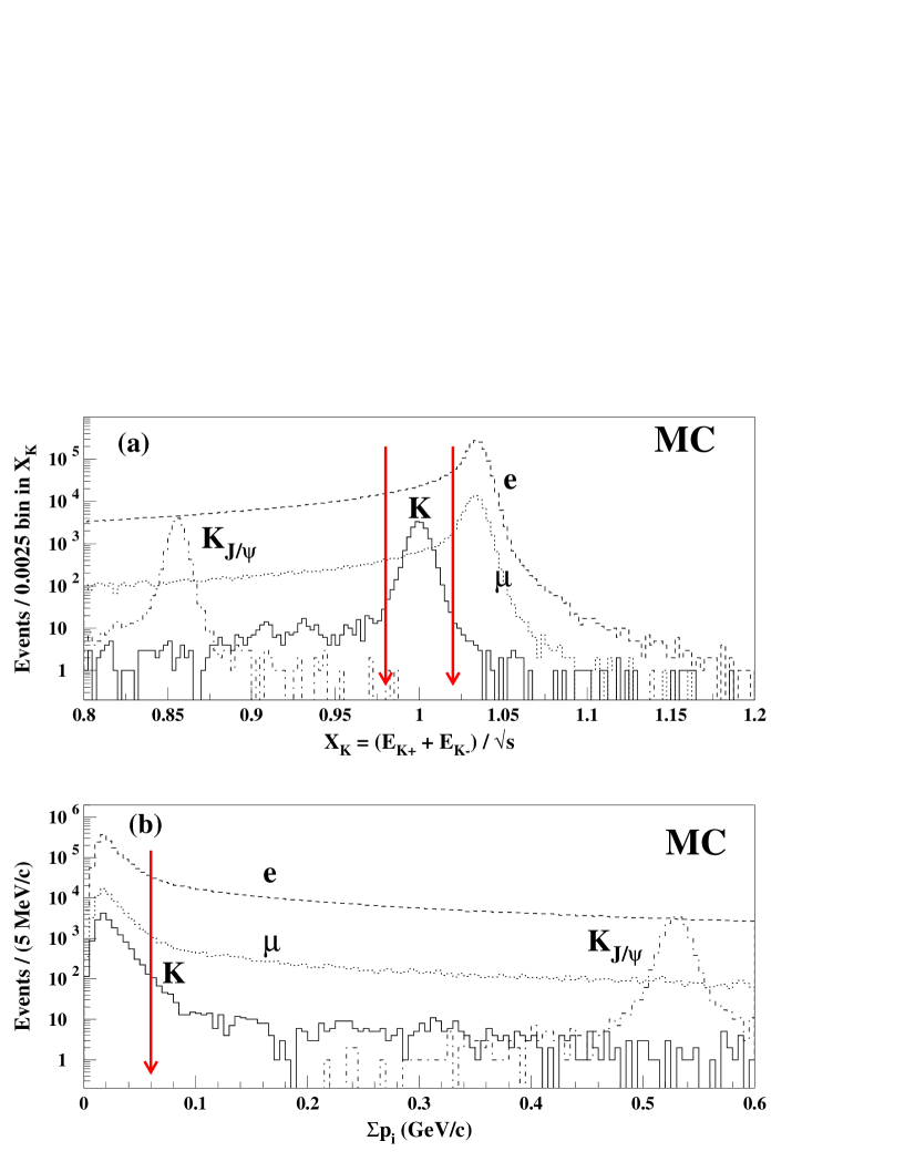
Figure 4.4: MC $X_{K}$ and net momentum ($\Sigma p_{i}$) distributions with acceptance, trigger, and tracking cuts applied. The solid histogram is $e^{+}e^{-}\rightarrow K^{+}K^{-}$ signal MC, the dot-dashed histogram is $e^{+}e^{-}\rightarrow\gamma J/\psi,J/\psi\rightarrow K^{+}K^{-}$ MC, the dashed histogram is Bhabha MC, and the dotted histogram is dimuon MC. The signal region is defined as 0.98 $<$ $X_{K}$ $<$ 1.02, designated by the arrows in Figure (a), and contains a very small contribution from $e^{+}e^{-}\rightarrow\gamma J/\psi,J/\psi\rightarrow K^{+}K^{-}$. A cut of $\Sigma p_{i}<$ 60 MeV/$c$ is applied to remove contributions from $e^{+}e^{-}\rightarrow\gamma J/\psi,J/\psi\rightarrow K^{+}K^{-}$. The $e^{+}e^{-}\rightarrow p\overline{p}$ and $e^{+}e^{-}\rightarrow\pi^{+}\pi^{-}$ processes have the same characteristics.

4.5 Event Selection $\&$ Backgrounds

4.5.1 Selection of $\pi^{+}\pi^{-}$ Events

Additional acceptance restrictions are applied to $\pi^{+}\pi^{-}$ final state events. They are

• Each track must have $|$cos$\theta$$|$ $<$ 0.75 (changed from 0.8)

• Each track must have an associated CC shower.

These extra requirements are necessary because the RICH detector endplates cover the barrel section of the CC for $|$cos$\theta$$|$ $>$ 0.75 and, since CC information is very important for the $\pi^{+}\pi^{-}$ analysis, the pion track must have an associated shower in the CC.

An additional restriction of $\Sigma p_{i}<$ 100 MeV/$c$ is used to select $\pi^{+}\pi^{-}$ events. This cut removes possible contamination from $J/\psi\rightarrow\pi^{+}\pi^{-}$ decays, as it did for the $K^{+}K^{-}$ final state events shown in Figure 4.4b.

The most important issue for the $\pi^{+}\pi^{-}$ analysis is how to distinguish a charged pion track from a muon when they have comparable momenta of $\sim$1.83 GeV/$c$. The track momenta are too high for using $dE/dx$ and RICH information and too low for the muon detector. The solution is to use the CC to distinguish pion tracks which interact hadronically, from muons which do not.

The muon rejection selection criterion is arbitrarily defined by requiring that there be $<$ 0.1 $\mu^{+}\mu^{-}$ final state events in the $\pi^{+}\pi^{-}$ signal region, either from $e^{+}e^{-}\rightarrow\mu^{+}\mu^{-}$, or $\psi(2S)\rightarrow\mu^{+}\mu^{-}$. The dimuon MC sample gives 55,361$\pm$235 $e^{+}e^{-}\rightarrow\mu^{+}\mu^{-}$ events in the $\pi^{+}\pi^{-}$ signal region after satisfying the acceptance, trigger, tracking criteria and $\Sigma p_{i}<$ 100 MeV/$c$. Note that the number of $\mu^{+}\mu^{-}$ events (consisting of both $e^{+}e^{-}\rightarrow\mu^{+}\mu^{-}$ and $\psi(2S)\rightarrow\mu^{+}\mu^{-}$ events) in the $\psi(2S)$ data sample is expected to be nearly half, or 26,189$\pm$1234. The lepton track fake rate efficiency is related to the total number of $l^{+}l^{-}$ events by

$$\epsilon_{l}=\sqrt{\frac{N_{l,bg}}{N_{l,total}}}.$$ (4.6)

For example, a contamination of 0.1 $\mu^{+}\mu^{-}$ events in the continuum $\pi^{+}\pi^{-}$ signal region would require an efficiency of $\epsilon_{\mu}=\sqrt{(0.1)/(55,361)}=1.3\times 10^{-3}$.

The muon detector cannot reject the dimuon background at the desired level of 0.1 events. The efficiency of the muon detector for muon tracks with momenta in the range 1.5-2.0 GeV/$c$ is $\sim$85$\%$ [173]. That corresponds to a muon track fake rate efficiency of $\epsilon_{\mu}$ = 15$\%$ or, using Eqn. 4.6, 1245 dimuon events. It is for this reason that more drastic muon rejection is required.

The muon track fake rate efficiency is determined using the dimuon MC sample. The positive and negative muon tracks are analyzed individually and the efficiencies are combined to determine the net efficiency. A candidate track satisfies the acceptance, trigger, and tracking criteria. The energy deposited in the CC from a muon track is shown in Figure 4.5a. Requiring a muon to have $E_{tkCC}$ $>$ 420 MeV has an efficiency of $\epsilon_{\mu}$ = (0.099$\pm$0.009)$\%$, which corresponds to 0.054$\pm$0.009 $e^{+}e^{-}\rightarrow\mu^{+}\mu^{-}$ events in the continuum data $\pi^{+}\pi^{-}$ signal region. This is a factor two better than our goal.

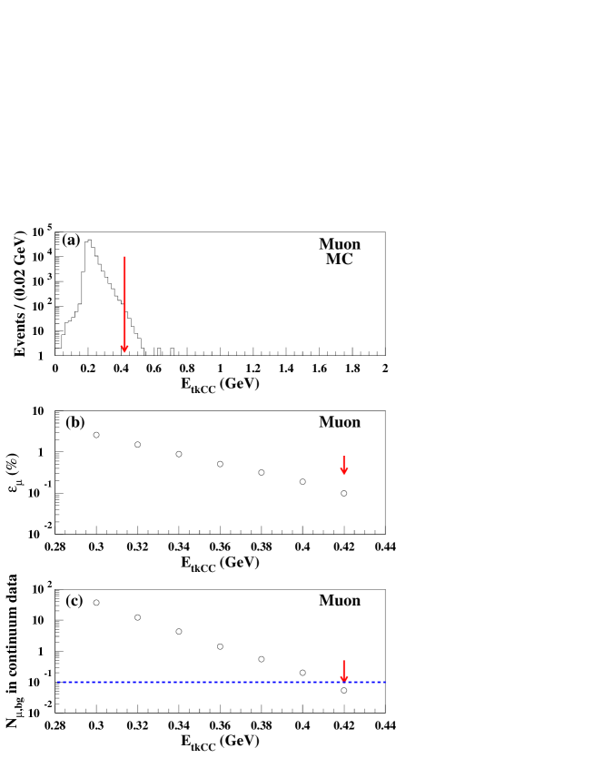
Figure 4.5: Figure (a): Shower energy deposited in the CC associated with a muon track from the dimuon MC sample. Figure (b): Muon track fake rate efficiency as a function of $E_{tkCC}$. Figure (c): Number of expected dimuon background events in the continuum data sample as a function of $E_{tkCC}$. The values on the abscissa of Figures (b) and (c) imply a cut selecting a candidate track with $E_{tkCC}$ greater than the value. Requiring the track to have $E_{tkCC}$ $>$ 420 MeV (denoted by the arrows) only allows 0.054$\pm$0.009 dimuon events in the continuum $\pi^{+}\pi^{-}$ signal region.

The behavior of hadronically-interacting pions in the CC is studied using data and MC samples with pion tracks having momenta of $\sim$1.83 GeV. Since there is no such sample of pion tracks taken with the CLEO-c detector, inclusive $D^{0}\rightarrow K^{-}\pi^{+}$ decays (charge conjugation is assumed) collected with the CLEO III detector are studied. The only differences between the CLEO-c and CLEO III detectors are that the inner drift chamber replaced a four-layer Silicon vertex detector and the solenoidal magnetic field was lowered to 1.0 Tesla from 1.5 Tesla. Since the main drift chamber, RICH detector, and CC are the same in both detectors, the properties of the pions studied using the CLEO III detector are consistent with those in the CLEO-c detector. More information on the CLEO III detector can be found in Ref. [193].

The sample of inclusive $D^{0}\rightarrow K^{-}\pi^{+}$ decays are from a $\sim$3.3 fb^-1 data sample taken at the $\Upsilon(4S)$ resonance ($\sqrt{s}$ $\sim$ 10.58 GeV). The $D^{0}\rightarrow K^{-}\pi^{+}$ MC samples, which corresponds to four times the $\Upsilon(4S)$ data sample, are from $\Upsilon(4S)$ $\rightarrow$ $B\overline{B}$ decays and $e^{+}e^{-}$ $\rightarrow$ $q\overline{q}$ events ($q$ = $u,d,s,c$). The $B$ mesons are decayed according to their branching fractions listed in the PDG [2]. The $e^{+}e^{-}$ $\rightarrow$ $q\overline{q}$ events produce hadrons according to the string fragmentation functions in the LUND/JETSET model [194, 195].

In order to get a clean sample of $D^{0}\rightarrow K^{-}\pi^{+}$ decays with lower background levels, the kaon candidate track is required to have $E_{tkCC}/p$ $<$ 0.85, $dE/dx$ $|S_{K}|$ $<$ 3 (see Eqn. 4.4), no associated signal in the muon detector, and $\Delta\chi^{2}(K-\pi)$ $<$ 0 (see Eqn. 4.5). The pion candidate tracks in this CC study are only required to satisfy the tracking criteria.

Figure 4.6 shows the pion $E_{tkCC}$ behavior from CLEO III data (solid curve, filled squares) and MC (dotted curve, open squares) $D^{0}\rightarrow K^{-}\pi^{+}$ events. They are consistent for pions with momenta of $\sim$1.83 GeV. Figure 4.6 also shows the $E_{tkCC}$ behavior for pions from the $e^{+}e^{-}\rightarrow\pi^{+}\pi^{-}$ signal MC sample (dashed curve), with the efficiency (open triangles) determined in the same manner as for the muon fake rate efficiency described above. The pion efficiency from the CLEO III $D^{0}\rightarrow K^{-}\pi^{+}$ sample is found to be $\sim$10$\%$ larger than that from the signal MC. The average of these two efficiency estimates is used in the present analysis for pions having $E_{tkCC}$ $>$ 420 MeV; the difference between them is assigned to the systematic uncertainty.

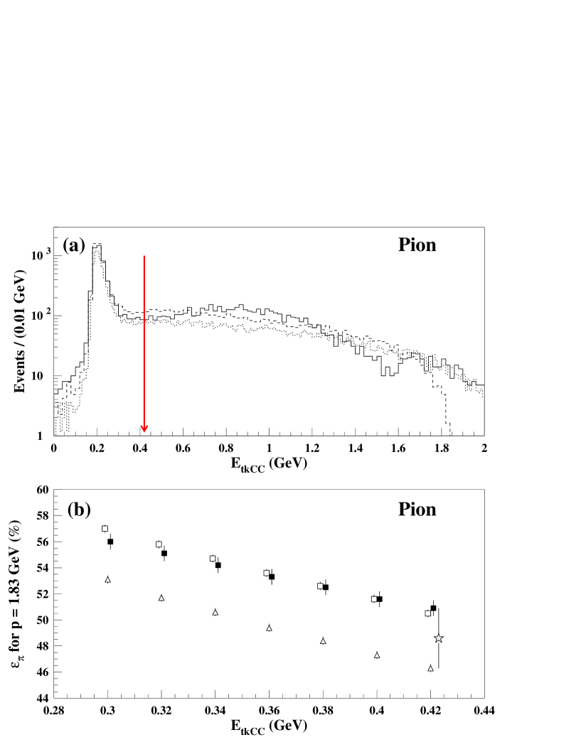
Figure 4.6: Figure (a): Pion $E_{tkCC}$ distributions from CLEO III $D^{0}\rightarrow K^{-}\pi^{+}$ data events (solid histogram), CLEO III $D^{0}\rightarrow K^{-}\pi^{+}$ MC events (dotted), and $e^{+}e^{-}\rightarrow\pi^{+}\pi^{-}$ signal MC (dashed). The arrow denotes the $E_{tkCC}$ $>$ 420 MeV cut. Figure (b): Pion efficiencies as a function of $E_{tkCC}$ from CLEO III $D^{0}\rightarrow K^{-}\pi^{+}$ data events (filled squares), CLEO III $D^{0}\rightarrow K^{-}\pi^{+}$ MC events (open squares), and signal MC (open triangles). The efficiency used in the present analysis is the average between the efficiencies from the CLEO III $D^{0}\rightarrow K^{-}\pi^{+}$ data events ($\blacksquare$) and the signal MC($\vartriangle$), with the difference between them assigned to systematic uncertainty, as shown by the open star. The star is displaced to clearly show its uncertainty.

The $e^{+}e^{-}$ final state events have unique characteristics which allow for easier rejection, but the sheer number of $e^{+}e^{-}$ events is formidable. The Bhabha MC sample consists of 1,164,559$\pm$1079 $e^{+}e^{-}$ events in the $\pi^{+}\pi^{-}$ signal region after satisfying the acceptance, trigger, and tracking criteria and $\Sigma p_{i}<$ 100 MeV/$c$ (there are 162,953$\pm$264 events in the $\psi(2S)$ data sample from both $e^{+}e^{-}\rightarrow e^{+}e^{-}$ and $\psi(2S)\rightarrow e^{+}e^{-}$ events). This requires an electron track fake rate efficiency of $\epsilon_{e}$ $<$ 9$\times 10^{-4}$ for $<$ 1 $e^{+}e^{-}$ event to contaminate the continuum $\pi^{+}\pi^{-}$ signal region. The easiest way to reject an electron track is require it to have an $E_{tkCC}/p$ $<$ 0.85. This is normally a sufficient cut, but is not adequate for the present analysis. The $E_{tkCC}/p$ $<$ 0.85 cut fails to remove Bhabha events when (a) the track goes between two crystals, or (b) ’hot’ or defective crystals are included in the CC shower. Additional rejection of $e^{+}e^{-}$ events is performed by using information from the $dE/dx$ and the RICH detector.

To study the rejection of electrons, radiative Bhabha events in the continuum data sample are used. We require that a candidate radiative Bhabha event should have $X_{\pi}$ $<$ 0.975, i.e., below the $\pi^{+}\pi^{-}$ signal region. The candidate electron track must have $|$cos$\theta|$ $<$ 0.75, satisfy the track quality and IP criteria, $p$ $>$ 1.6 GeV, and 0.7 $<$ $E_{tkCC}/p$ $<$ 1.1, while the other track must have 0.85 $<$ $E_{tkCC}/p$ $<$ 1.1, and $dE/dx$ $S_{e}$ $>$ -2 (see Eqn. 4.4 for definition of $S_{e}$). Figures 4.7a and Figures 4.7b show the $E_{tkCC}/p$ and $\Delta\chi^{2}(\pi-e)$ distributions for the candidate Bhabha track, respectively. Figure 4.7c shows the $\Delta\chi^{2}(\pi-e)$ distribution for the positive track from the $e^{+}e^{-}\rightarrow\pi^{+}\pi^{-}$ signal MC sample. A total number of 556,902 radiative Bhabha events survive the above criteria. Of these events, 4282$\pm$65 candidate electron tracks have an $E_{tkCC}/p$ between 0.7 and 0.85, or $\epsilon_{e}$ = (7.69$\pm$0.12)$\times 10^{-3}$. This fake rate efficiency corresponds to $\sim$69 $e^{+}e^{-}$ events in the $\pi^{+}\pi^{-}$ signal region for the continuum data sample. The additional requirement of $\Delta\chi^{2}(\pi-e)<$ 0 reduces the number of candidate electron tracks to 120$\pm$11 with $\epsilon_{e}$ = (2.15$\pm$0.20)$\times 10^{-4}$, which gives 0.054$\pm$0.010 $e^{+}e^{-}$ events in the continuum data $\pi^{+}\pi^{-}$ signal region.

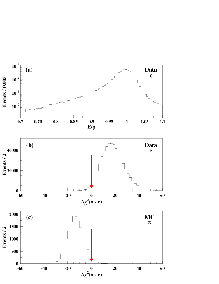
Figure 4.7: Distributions from the continuum data radiative Bhabha and $e^{+}e^{-}\rightarrow\pi^{+}\pi^{-}$ signal MC samples. Figure (a): $E_{tkCC}/p$ for the candidate track from the radiative Bhabha sample. Figure (b): $\Delta\chi^{2}(\pi-e)$ for the candidate track from the radiative Bhabha sample. Figure (c): $\Delta\chi^{2}(\pi-e)$ for the positive track from the $e^{+}e^{-}\rightarrow\pi^{+}\pi^{-}$ signal MC.

By requiring each track in an event to have $E_{tkCC}$ $>$ 420 MeV, $E_{tkCC}/p$ $<$ 0.85, and $\Delta\chi^{2}(\pi-e)$ $<$ 0, the number of $l^{+}l^{-}$ background events in the continuum and $\psi(2S)$ data samples are $N^{cont}_{l^{+}l^{-}}$ = 0.108$\pm$0.013 and $N^{\psi(2S)}_{l^{+}l^{-}}$ = 0.021$\pm$0.003, respectively.

From Figure 4.1, we note that a small number of $K^{+}K^{-}$ final state events can enter the $\pi^{+}\pi^{-}$ signal region. From the $e^{+}e^{-}\rightarrow K^{+}K^{-}$ signal MC, 0.73$\%$ of all $K^{+}K^{-}$ events which satisfy the acceptance, trigger, and tracking criteria populate the $\pi^{+}\pi^{-}$ signal region. As will be shown in the Results section (Section 4.8.5), approximately 100 observed $K^{+}K^{-}$ final state events are found in both $\psi(2S)$ and continuum data samples. Therefore, $\sim$0.73 events in the $\pi^{+}\pi^{-}$ signal region can be from charged kaon pairs. The efficiency for kaon-faking-pion with $\Delta\chi^{2}(\pi-K)$ $<$ 0 is determined to be 2.5$\%$ from the $e^{+}e^{-}\rightarrow K^{+}K^{-}$ signal MC. The $\Delta\chi^{2}(\pi-K)$ cut reduces the $K^{+}K^{-}$ background to (0.73)(0.025)² = 0.0005 events and can be safely neglected.

Table 4.2 lists the efficiencies for the $\pi^{+}\pi^{-}$ final state criteria. The signal MC samples are used to determine the efficiency except for the efficiency associated with the $E_{tkCC}$ criterion. The efficiency for the track $E_{tkCC}$ is determined from an average of the $e^{+}e^{-}\rightarrow\pi^{+}\pi^{-}$ signal MC and the CLEO III $D^{0}\rightarrow K^{-}\pi^{+}$ data samples. The total efficiency for the $\pi^{+}\pi^{-}$ final state is $\epsilon_{tot}$ = 0.166 $\pm$ 0.013.

Table 4.2: Efficiencies for the $\pi^{+}\pi^{-}$ final state. The individual efficiencies (1-7) are determined with respect to the acceptance cuts.

Cuts	Requirement	$\epsilon$
Acceptance	Ntrk = 2
	$\Sigma Q$ = 0	0.861
	$|$cos($\theta_{tk}$)$|$ $<$ 0.75
1. Trigger	L1 Trigger = TRUE	0.997
2. IP	$|d_{b}|$ $<$ 5 mm	0.999
	$|z_{b}|$ $<$ 5 cm
3. Track Quality	0.5 $<$ DRHF $<$ 1.2	0.9997
	$\chi^{2}/dof$ $<$ 10
4. $X_{\pi}$ = ($E_{\pi^{+}}$+$E_{\pi^{-}}$)/$\sqrt{s}$	0.98 $<$ $X_{\pi}$ $<$ 1.02	0.940
5. Net Momentum	$\Sigma p_{i}$ $<$ 100 MeV/$c$	0.947
6. $\pi-K$ Separation	$\Delta\chi^{2}(\pi-K)$ $<$ 0	0.966
7. $\pi-e$ Separation	$E_{tkCC}/p$ $<$ 0.85	0.957
	$\Delta\chi^{2}(\pi-e)$ $<$ 0	0.945
$\epsilon_{MC}$	Acc + Cuts 1-7	0.702(3)
$\pi-\mu$ Separation: $\epsilon_{\pi}(E_{tkCC})$	$E_{tkCC}$ $>$ 420 MeV	0.486(3)
$\epsilon_{tot}$	$\epsilon_{MC}*(\epsilon_{\pi}(E_{tkCC}))^{2}$	0.166(2)

The generic $\psi(2S)$ MC sample is analyzed to test for other backgrounds which satisfy the $\pi^{+}\pi^{-}$ final state criteria. In the 40,568,651 generic $\psi(2S)$ decays, there are 3436 $\psi(2S)\rightarrow\pi^{+}\pi^{-}$ decays. After applying the selection criteria, only one background event is found in the $\pi^{+}\pi^{-}$ signal region. The one background event is found to be from a $\psi(2S)\rightarrow\mu^{+}\mu^{-}$ decay. This is consistent with the dimuon rejection determined above. The $\psi(2S)\rightarrow\pi^{+}\pi^{-}$ branching ratio is not determined from this MC sample because of the issues discussed at the end of Section 4.2.

Figures 4.8a and 4.9a show the $X_{\pi}$ distributions for the $\psi(2S)$ and continuum data, respectively, after applying all $\pi^{+}\pi^{-}$ final state criteria except for the net momentum criterion. The P-wave spin triplet charmonium resonances $\chi_{c0}$ and $\chi_{c2}$ are seen in the $\psi(2S)$ data, but they are outside of the $X_{\pi}$ signal region. Figure 4.8b shows that only $\psi(2S)\rightarrow\pi^{+}\pi^{-}$ events survive after applying the net momentum criterion, and Figure 4.9b shows that only $e^{+}e^{-}\rightarrow\pi^{+}\pi^{-}$ events survive after applying the net momentum criterion.

Figure 4.10a shows the $X_{\pi}$ signal region and the vicinity after the $\pi^{+}\pi^{-}$ final state criteria are applied to the $e^{+}e^{-}\rightarrow h\overline{h}$ signal and $e^{+}e^{-}\rightarrow l^{+}l^{-}$ MC samples. Only one background event is in MC $X_{\pi}$ signal region, which comes from the $e^{+}e^{-}\rightarrow\mu^{+}\mu^{-}$ MC sample. Figures 4.10b and 4.10c show the $X_{\pi}$ distributions after the $e^{+}e^{-}\rightarrow\pi^{+}\pi^{-}$ selection criteria have been applied to the $\psi(2S)$ and continuum data samples, respectively. In both cases, 1-3 $\psi(2S)\rightarrow p\overline{p}$ events around $X_{\pi}$ = 0.85 are observed, far away from the $\pi^{+}\pi^{-}$ signal region.

Figure 4.8: Effect of net momentum criterion on the $\psi(2S)$ data for the $\pi^{+}\pi^{-}$ final state. Figure (a) shows the $\psi(2S)$ data after applying all $\pi^{+}\pi^{-}$ final state criteria except for the net momentum criterion, while Figure (b) includes it. The $\chi_{c0}$ and $\chi_{c2}$ are clearly seen in Figure (a) at $X_{\pi}$ = 0.926 and 0.965, respectively, outside of the 0.98 $<$ $X_{\pi}$ $<$ 1.02 signal region, and are removed in Figure (b) due to the net momentum criterion.

Figure 4.9: Effect of net momentum criterion on the continuum data for the $\pi^{+}\pi^{-}$ final state. Figure (a) shows the continuum data after applying all $\pi^{+}\pi^{-}$ final state criteria except for the net momentum criterion, while Figure (b) includes it. The net momentum criterion removes events below the signal region.

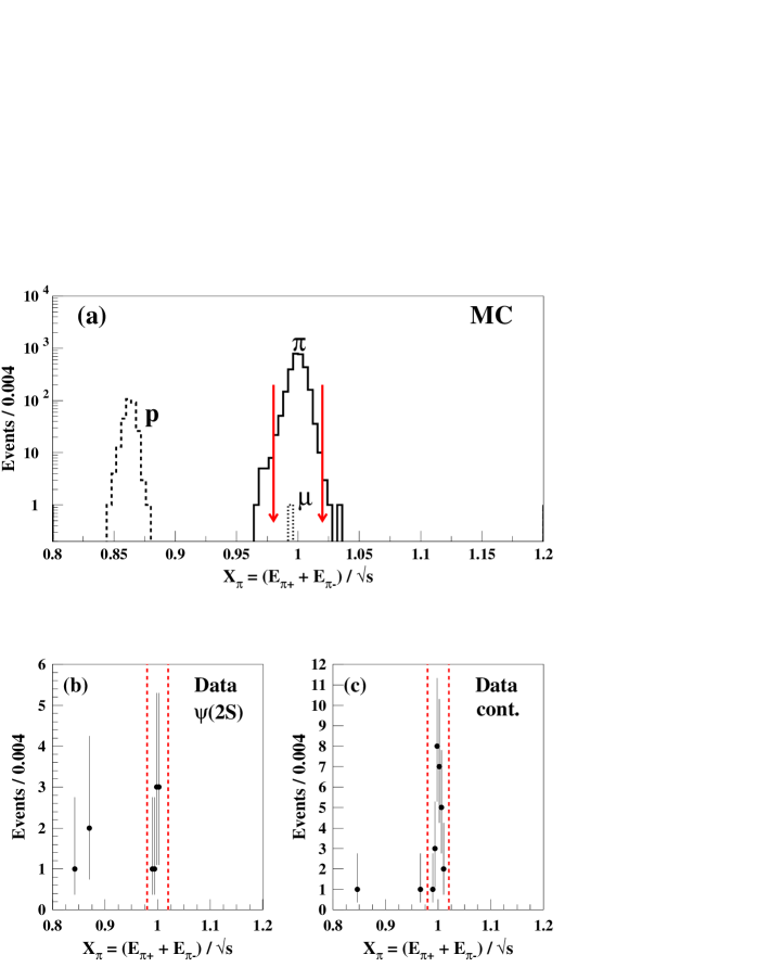
Figure 4.10: MC and data $X_{\pi}$ distributions for events which satisfy the $\pi^{+}\pi^{-}$ final state criteria. The arrows in Figure (a) and the dashed lines in Figures (b) and (c) denote the signal region of 0.98 $<$ $X_{\pi}$ $<$ 1.02. The solid histogram in Figure (a) is $e^{+}e^{-}\rightarrow\pi^{+}\pi^{-}$ signal MC, the dotted histogram is dimuon MC, and the dashed histogram is $e^{+}e^{-}\rightarrow p\overline{p}$ signal MC obtained with $|G^{P}_{E}(s)|$ = 0. Figure (b) is for the $\psi(2S)$ data sample. Figure (c) is for the continuum data sample. There are 8 events in the $\psi(2S)$ signal region and 26 events in the continuum signal region.

4.5.2 Selection of $K^{+}K^{-}$ Events

As can be seen in Figure 4.2, the $K^{+}K^{-}$ final state signal region is displaced from the main $e^{+}e^{-}\rightarrow l^{+}l^{-}$ background, but it still contains a sizeable amount of leptonic background events. The net momentum constraint and PID information from $dE/dx$ and the RICH detector are extremely important for suppressing the leptonic background in the $K^{+}K^{-}$ final state analysis.

The net momentum of the $K^{+}K^{-}$ pair and the leptonic background in the $K^{+}K^{-}$ signal region are shown in Figure 4.11b. The leptonic background peaks around $\Sigma p_{i}\sim$ 0.8 GeV/$c$, so a cut is applied requiring $\Sigma p_{i}<$ 0.6 GeV/$c$ and has an efficiency of 93$\%$.

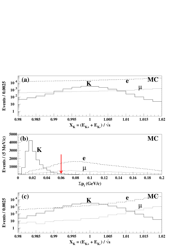
Figure 4.11: MC distributions in the $K^{+}K^{-}$ signal region with acceptance, trigger, and tracking cuts applied. The solid histogram is $e^{+}e^{-}\rightarrow K^{+}K^{-}$ signal MC, the dashed histogram is Bhabha MC, and the dotted histogram is dimuon MC. Figure (a) is the $X_{K}$ signal region, and Figure (b) is the net monemtum ($\Sigma p_{i}$) of the two tracks. The Bhabha MC sample in Figure (b) has been decreased by a factor of 10 to show more detail. A cut is be applied at $\Sigma p_{i}$ $<$ 60 MeV/$c$ to remove contamination from the leptonic background. Figure (c) is the $X_{K}$ signal region after applying the $\Sigma p_{i}$ $<$ 60 MeV/$c$ cut.

The PID criteria for the $K^{+}K^{-}$ final state is determined from a signal squared to signal plus background ($S^{2}/(S+B)$) study. The signal is from the $e^{+}e^{-}\rightarrow K^{+}K^{-}$ signal MC sample and the background is from the continuum data sample. The background data sample satisfies the following criteria: 1.025 $<$ $X_{K}$ $<$ 1.07, with each track having $E_{tkCC}/p$ $<$ 0.7 for the $e^{+}e^{-}\rightarrow\mu^{+}\mu^{-}$ sample and $E_{tkCC}/p$ $>$ 0.7 for the $e^{+}e^{-}\rightarrow e^{+}e^{-}$ sample. Figure 4.12 shows the $S^{2}/(S+B)$ distributions for different values of $\Delta\chi^{2}(K-l)$ applied (for the definition of $\Delta\chi^{2}$, see Eqn. 4.5). The effect of applying an additional cut on $E_{tkCC}/p$ $<$ 0.85 is also considered for rejection of the $e^{+}e^{-}\rightarrow e^{+}e^{-}$ background. Applying the $E_{tkCC}/p$ cut improves the $S^{2}/(S+B)$ ratio as compared to only requiring $\Delta\chi^{2}(K-e)$. The $S^{2}/(S+B)$ studies suggest cuts of $E_{tkCC}/p$ $<$ 0.85, $\Delta\chi^{2}(K-e)$ $<$ 0, and $\Delta\chi^{2}(K-\mu)$ $<$ -2 for each track.

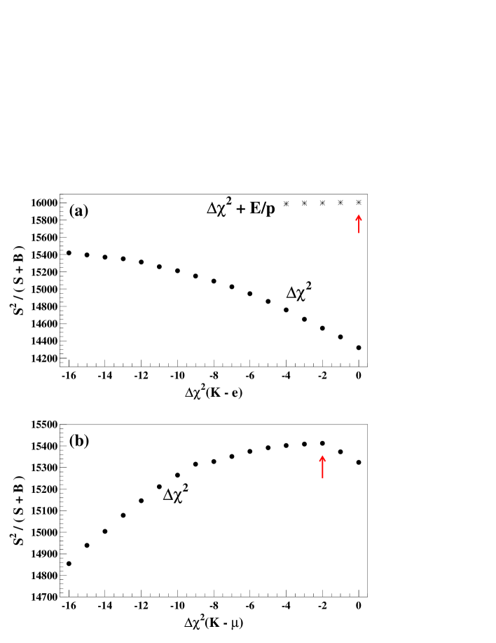
Figure 4.12: Kaon PID $S^{2}/(S+B)$ study. The values on the abscissa imply a cut on $\Delta\chi^{2}(K-l)$ less than the value. The signal (S) used in both figures is from the $e^{+}e^{-}\rightarrow K^{+}K^{-}$ signal MC. The background (B) in Figure (a) is from $e^{+}e^{-}\rightarrow e^{+}e^{-}$ sideband data. The solid points in Figure (a) only have the $\Delta\chi^{2}(K-e)$ cut applied, while the star points have an additional cut of $E_{tkCC}/p$ $<$ 0.85 applied. The background (B) in Figure (b) is from $e^{+}e^{-}\rightarrow\mu^{+}\mu^{-}$ sideband data. The study suggests cuts of $E_{tkCC}/p$ $<$ 0.85 and $\Delta\chi^{2}(K-e)$ $<$ 0 (arrow in Figure (a)) and a cut of $\Delta\chi^{2}(K-\mu)$ $<$ -2 (arrow in Figure (b)) on each track.

Table 4.3 lists the individual and total efficiencies from the $e^{+}e^{-}\rightarrow K^{+}K^{-}$ signal MC sample. The total efficiency for the $K^{+}K^{-}$ final state is $\epsilon_{tot}$ = 0.743 $\pm$ 0.003.

Table 4.3: Efficiencies for the $K^{+}K^{-}$ final state. The individual efficiencies (1-7) are determined with respect to the acceptance cuts.

Cuts	Requirement	$\epsilon$
	Ntrk = 2
Acceptance	$\Sigma Q$ = 0	0.868
	$|$cos$(\theta_{tk})|$ $<$ 0.8
1. Trigger	L1 Trigger = TRUE	0.996
2. $X_{K}$ = ($E_{K^{+}}$+$E_{K^{-}}$)/$\sqrt{s}$	0.98 $<$ $X_{K}$ $<$ 1.02	0.948
3. IP	$|d_{b}|$ $<$ 5 mm	0.992
	$|z_{b}|$ $<$ 5 cm
4. Track Quality	0.5 $<$ DRHF $<$ 1.2	0.986
	$\chi^{2}/dof$ $<$ 10
5. Net Momentum	$\Sigma p_{i}$ $<$ 60 MeV/$c$	0.931
6. $K-e$ Separation	$E_{tkCC}/p$ $<$ 0.85	0.941
	$\Delta\chi^{2}(K-e)$ $<$ 0
7. $K-\mu$ Separation	$\Delta\chi^{2}(K-\mu)$ $<$ -2	0.923
$\epsilon_{tot}$	Acc + Cuts 1-7	0.743(3)

The generic $\psi(2S)$ MC sample is analyzed to test for other backgrounds which satisfy the $K^{+}K^{-}$ final state criteria. In the 40,568,651 generic $\psi(2S)$ decays, there are only 872 $\psi(2S)\rightarrow K^{+}K^{-}$ decays. After applying the $K^{+}K^{-}$ selection criteria, 486 $\psi(2S)\rightarrow K^{+}K^{-}$ events survive. The $\psi(2S)\rightarrow K^{+}K^{-}$ branching ratio is not determined from this MC sample because of the issues discussed at the end of Section 4.2.

Figures 4.13a and 4.14a show the $\psi(2S)$ and continuum data $X_{K}$ distributions, respectively, after applying all $K^{+}K^{-}$ final state criteria except for the net momentum criterion. The charmonium resonances $J/\psi$, $\chi_{c0}$, and $\chi_{c2}$ are seen in the $\psi(2S)$ data, but they are outside of the $X_{K}=0.98-1.02$ signal region. Figure 4.13b shows that only $\psi(2S)\rightarrow K^{+}K^{-}$ events survive after applying the net momentum criterion, and Figure 4.14b shows that only $e^{+}e^{-}\rightarrow K^{+}K^{-}$ events survive after applying the net momentum criterion.

Figure 4.13: Effect of net momentum criterion on the $\psi(2S)$ data for the $K^{+}K^{-}$ final state. Figure (a) shows the $\psi(2S)$ data after applying all $K^{+}K^{-}$ final state criteria except for the net momentum criterion, while Figure (b) includes it. The J/$\psi$, $\chi_{c0}$, and $\chi_{c2}$ are clearly seen in Figure (a) at $X_{K}$ = 0.840, 0.926, and 0.965, respectively, outside of the 0.98 $<$ $X_{K}$ $<$ 1.02 signal region, and are removed in Figure (b) due to the net momentum criterion.

Figure 4.14: Effect of net momentum criterion on the continuum data for the $K^{+}K^{-}$ final state. Figure (a) shows the continuum data after applying all $K^{+}K^{-}$ final state criteria except for the net momentum criterion, while Figure (b) includes it. The net momentum criterion removes events below the 0.98 $<$ $X_{K}$ $<$ 1.02 signal region but has no effect on the $e^{+}e^{-}\rightarrow l^{+}l^{-}$ events near $X_{K}$ = 1.03.

Figure 4.15a shows the $X_{K}$ signal region and the vicinity after the $K^{+}K^{-}$ final state criteria are applied to the $e^{+}e^{-}\rightarrow h\overline{h}$ signal and $e^{+}e^{-}\rightarrow l^{+}l^{-}$ MC samples. Only $e^{+}e^{-}\rightarrow K^{+}K^{-}$ MC events populate the signal region. Figures 4.15b and 4.15c show the $X_{K}$ distributions after the $e^{+}e^{-}\rightarrow K^{+}K^{-}$ selection criteria have been applied to the $\psi(2S)$ and continuum data samples, respectively. In both cases, a small number of $\psi(2S)\rightarrow p\overline{p}$ events around $X_{K}$ = 0.9 are observed, far away from the $K^{+}K^{-}$ signal region. The presence of events around $X_{K}$ = 1.03 is consistent with the leptonic background. The determination of the $l^{+}l^{-}$ contamination in the $K^{+}K^{-}$ signal region is discussed below.

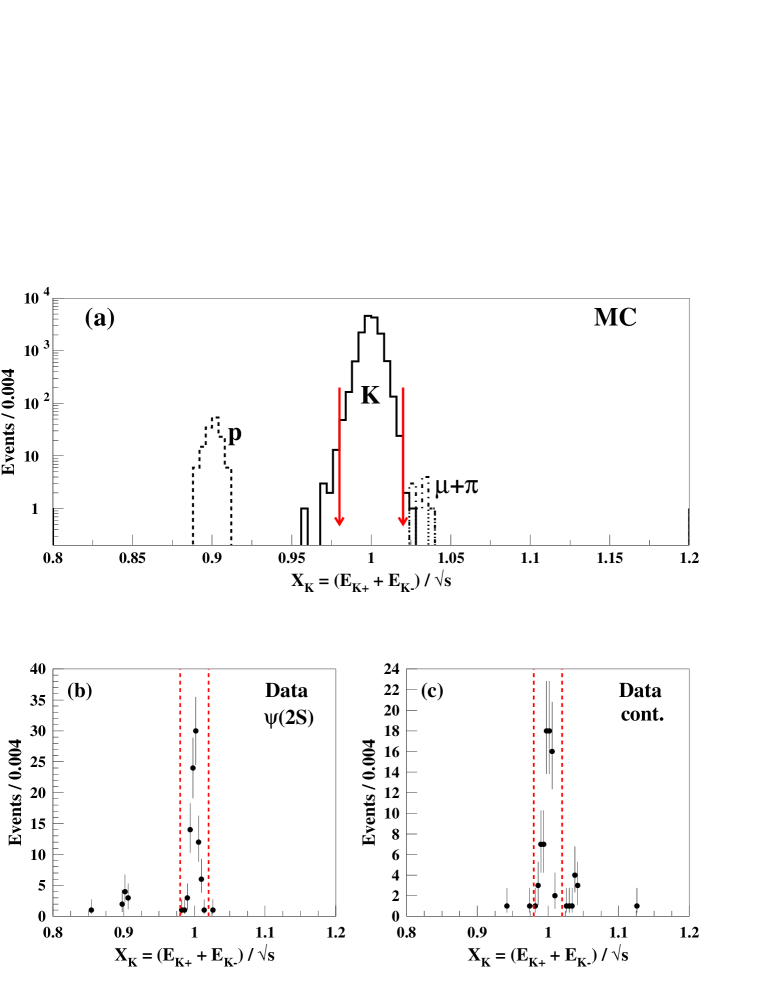
Figure 4.15: MC and data $X_{K}$ distributions for events which satisfy the $K^{+}K^{-}$ final state event selection criteria. The arrows in Figure (a) and the dashed lines in Figures (b) and (c) denote the signal region of 0.98 $<$ $X_{K}$ $<$ 1.02. The solid histogram in Figure (a) is $e^{+}e^{-}\rightarrow K^{+}K^{-}$ signal MC, the dotted histogram is dimuon MC, the dot-dashed histogram is the $e^{+}e^{-}\rightarrow\pi^{+}\pi^{-}$ signal MC, and the dashed histogram is the $e^{+}e^{-}\rightarrow p\overline{p}$ signal MC obtained with $|G^{P}_{E}(s)|$ = 0 . Figure (b) is for the $\psi(2S)$ data sample. Figure (c) is for the continuum data sample. There are 92 events in the $\psi(2S)$ signal region and 72 events in the continuum signal region.

The $l^{+}l^{-}$ contamination is determined by a ratio of the number of $l^{+}l^{-}$ events from the leptonic MC samples without applying the kaon PID criteria. We determine the $l^{+}l^{-}$ events inside the $K^{+}K^{-}$ signal region and in the peak region of $e^{+}e^{-}\rightarrow l^{+}l^{-}$ production, namely 1.02 $<$ $X_{K}$ $<$ 1.07. The ratio of the two gives the leptonic MC scale factor

$$\frac{N^{l^{+}l^{-}}_{MC}(0.98<X_{K}<1.02)}{N^{l^{+}l^{-}}_{MC}(1.02<X_{K}<1.07)}=\frac{84378\pm 290}{1495073\pm 1223}=0.0564\pm 0.0002.$$

We scale the number of events in the $l^{+}l^{-}$ peak region, 1.02 $<$ $X_{K}$ $<$ 1.07, in the data samples with this ratio. The number of events in the $l^{+}l^{-}$ peak region from the continuum data sample is 10.00${}^{+3.81}_{-3.22}$. Therefore, the leptonic background in the $K^{+}K^{-}$ signal region is determined to be $N^{cont}_{l^{+}l^{-}}$ = 0.56${}^{+0.21}_{-0.18}$. The number of events in the $l^{+}l^{-}$ peak region from the $\psi(2S)$ data sample is 1.00${}^{+1.75}_{-0.63}$. Therefore, the leptonic background in the $K^{+}K^{-}$ signal region is determined to be $N^{\psi(2S)}_{l^{+}l^{-}}$ = 0.06${}^{+0.10}_{-0.04}$.

4.5.3 Selection of $p\overline{p}$ Events

Even though the $p\overline{p}$ final state signal region is substantially displaced from the $e^{+}e^{-}\rightarrow l^{+}l^{-}$ peak region, contamination from the leptonic background still exists. Constraining the net momentum of the $p\overline{p}$ pair and particle identification based on $dE/dx$ and RICH information are used to suppress the leptonic background.

The net momentum of the $p\overline{p}$ pair and the leptonic background in the $p\overline{p}$ signal region is shown in Figure 4.16. Requiring $\Sigma p_{i}<$ 100 MeV/$c$ removed a substantial portion of the leptonic background and has an efficiency of $>$ 98$\%$.

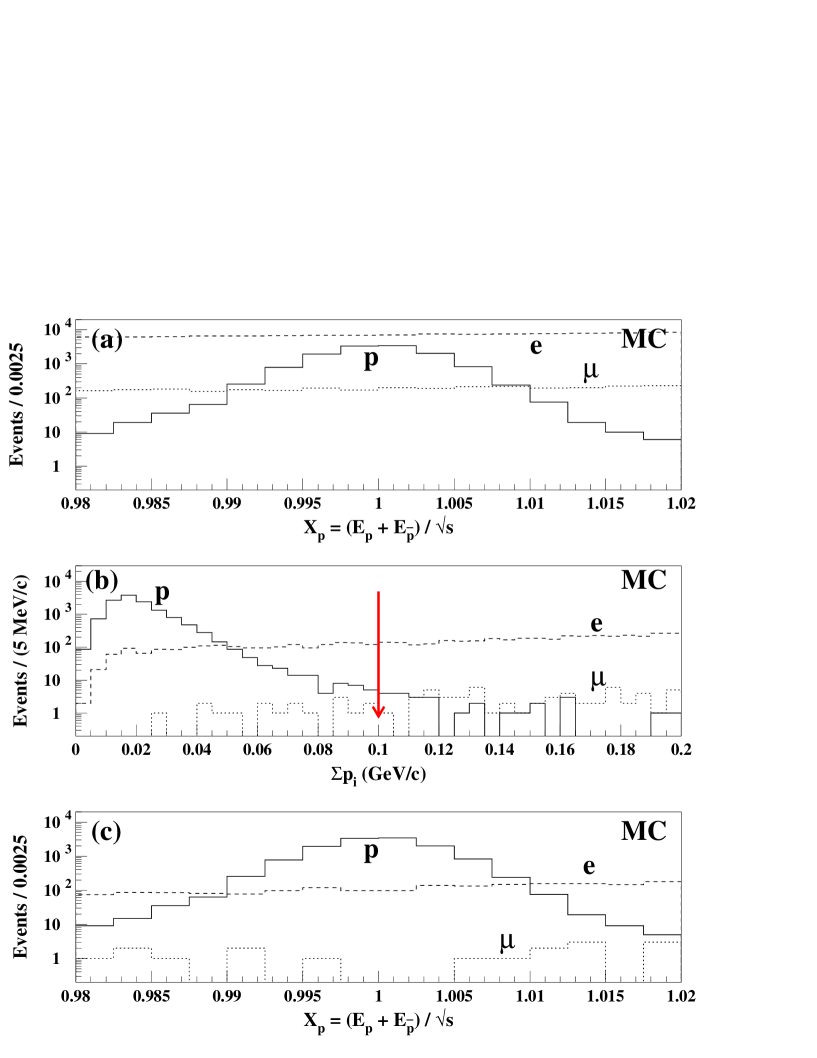
Figure 4.16: MC distributions in the $p\overline{p}$ signal region with acceptance, trigger, and tracking cuts applied. The solid histogram is the $e^{+}e^{-}\rightarrow p\overline{p}$ signal MC obtained with $|G^{P}_{E}(s)|$ = 0, the dashed histogram is Bhabha MC, and the dotted histogram is dimuon MC. Figure (a) is the $X_{p}$ signal region, and Figure (b) is the net monemtum ($\Sigma p_{i}$) of the two tracks. A cut is be applied at $\Sigma p_{i}$ $<$ 100 MeV/$c$ to remove contamination from the leptonic background. Figure (c) is the $X_{p}$ signal region after applying the $\Sigma p_{i}$ $<$ 100 MeV/$c$ cut.

The PID criteria for the $p\overline{p}$ final state is determined from a $S^{2}/(S+B)$ study. The signal is from the $e^{+}e^{-}\rightarrow p\overline{p}$ signal MC sample obtained with $|G^{P}_{E}(s)|$ = 0 and the background is from the continuum data sample. The background data sample satisfies the following criteria: 1.109 $<$ $X_{p}$ $<$ 1.155, with each track having $E_{tkCC}/p$ $<$ 0.7 for the $e^{+}e^{-}\rightarrow\mu^{+}\mu^{-}$ sample and $E_{tkCC}/p$ $>$ 0.7 for the $e^{+}e^{-}\rightarrow e^{+}e^{-}$ sample. Figure 4.17 shows the $S^{2}/(S+B)$ distributions for different values of $\Delta\chi^{2}(p-l)$ applied (for the definition of $\Delta\chi^{2}$, see Eqn. 4.5). The effect of applying an additional cut of $E_{tkCC}/p$ $<$ 0.85 is also considered for rejection of the $e^{+}e^{-}\rightarrow e^{+}e^{-}$ background. Applying the $E_{tkCC}/p$ cut to the proton candidate track improves the $S^{2}/(S+B)$ ratio but is worse for the antiproton candidate, as compared to only requiring $\Delta\chi^{2}(p-e)$. The reason is that the antiproton occasionally annihilates in the calorimeter. This has the effect of creating a broad bump in the $E_{tkCC}/p$ distribution ranging from 0.4 to 2.0. The $S^{2}/(S+B)$ studies suggest cuts of $\Delta\chi^{2}(p-e)$ $<$ 0 and $\Delta\chi^{2}(p-\mu)$ $<$ -2 for each track, with the additional cut of $E_{tkCC}/p$ $<$ 0.85 for the positive track.

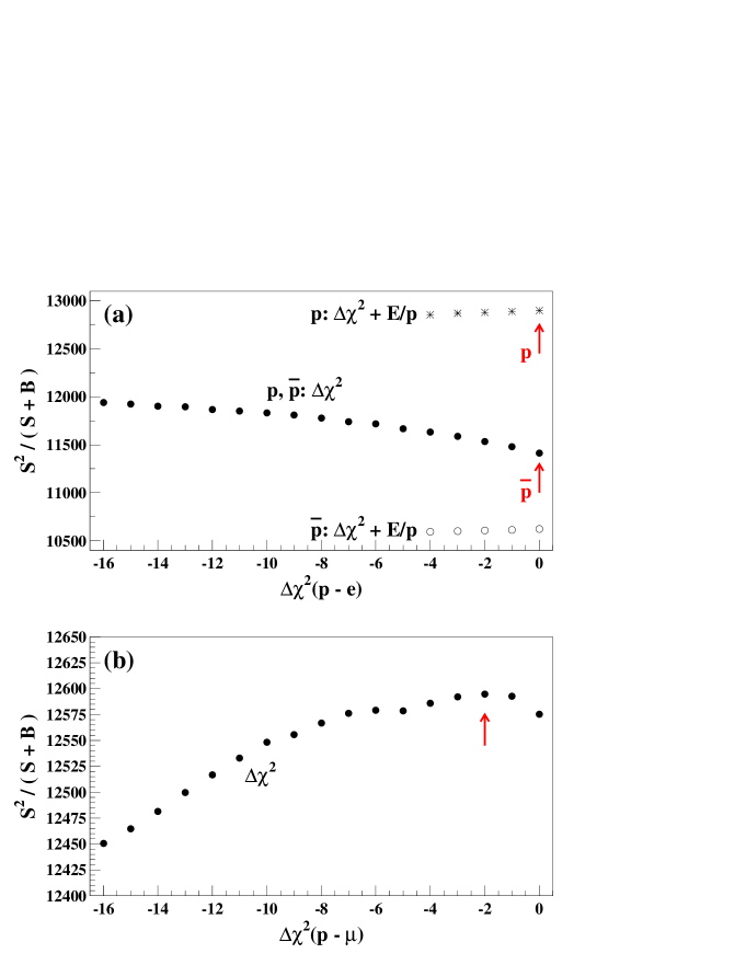
Figure 4.17: Proton PID $S^{2}/(S+B)$ study. The values on the abscissa imply a cut on $\Delta\chi^{2}(p-l)$ less than the value. The signal (S) used in both figures is from the $e^{+}e^{-}\rightarrow p\overline{p}$ signal MC obtained with $|G^{P}_{E}(s)|$ = 0 . The background (B) in Figure (a) is from $e^{+}e^{-}\rightarrow e^{+}e^{-}$ sideband data. The solid points in Figure (a) only have the $\Delta\chi^{2}(p-e)$ cut applied, the star points correspond to an additional cut of $E_{tkCC}/p$ $<$ 0.85 applied to the positive (proton) track, and the open points correspond to an additional cut of $E_{tkCC}/p$ $<$ 0.85 applied to the negative (antiproton) track. The background (B) in Figure (b) is from $e^{+}e^{-}\rightarrow\mu^{+}\mu^{-}$ sideband data. The study suggests cuts of $E_{tkCC}/p$ $<$ 0.85 and $\Delta\chi^{2}(p-e)$ $<$ 0 for the positive track and only $\Delta\chi^{2}(p-e)$ $<$ 0 for the negative track (arrows in Figure (a)). It also suggests a cut of $\Delta\chi^{2}(p-\mu)$ $<$ -2 (arrow in Figure (b)) on each track.

Table 4.4 lists the individual and total efficiencies determined from the $e^{+}e^{-}\rightarrow p\overline{p}$ signal MC samples. The total efficiency for the $p\overline{p}$ final state, assuming $|G^{P}_{E}(s)|$ = 0, is $\epsilon_{tot}$ = 0.626 $\pm$ 0.003 and, assuming $|G^{P}_{E}(s)|$ = $|G^{P}_{M}(s)|$, is $\epsilon_{tot}$ = 0.657 $\pm$ 0.003.

Table 4.4: Efficiencies for the $p\overline{p}$ final state determined from the $|G^{P}_{E}(s)|$ = 0 and $|G^{P}_{E}(s)|$ = $|G^{P}_{M}(s)|$ $e^{+}e^{-}\rightarrow p\overline{p}$ signal MC samples. The individual efficiencies (1-7) are determined with respect to the acceptance cuts.

Cuts	Requirement	$\epsilon$	$\epsilon$
		$(\frac{|G^{P}_{E}(s)|}{|G^{P}_{M}(s)|}=0)$	$(\frac{|G^{P}_{E}(s)|}{|G^{P}_{M}(s)|}=1)$
	Ntrk = 2
Acceptance	$\Sigma Q$ = 0	0.666	0.704
	$|$cos$(\theta_{tk}|$ $<$ 0.8
1. Trigger	L1 Trigger = TRUE	0.998	0.997
2. $X_{p}$ = ($E_{p}$+$E_{\overline{p}}$)/$\sqrt{s}$	0.98 $<$ $X_{p}$ $<$ 1.02	0.987	0.982
3. IP	$|d_{b}|$ $<$ 5 mm	0.999	0.998
	$|z_{b}|$ $<$ 5 cm
4. Track Quality	0.5 $<$ DRHF $<$ 1.2	0.9997	0.9995
	$\chi^{2}/dof$ $<$ 10
5. Net Momentum	$\Sigma p_{i}$ $<$ 100 MeV/$c$	0.986	0.981
6. $p-e$ Separation	$E_{tkCC}/p$ $<$ 0.85 (+ track)	0.978	0.976
	$\Delta\chi^{2}(p-e)$ $<$ 0
7. $p-\mu$ Separation	$\Delta\chi^{2}(p-\mu)$ $<$ -2	0.959	0.958
$\epsilon_{tot}$	Acc + Cuts 1-7	0.626(3)	0.657(3)

The generic $\psi(2S)$ MC sample is analyzed to test for other backgrounds which satisfy the $p\overline{p}$ final state criteria. In the 40,568,651 generic $\psi(2S)$ decays, there are only 1778 $\psi(2S)\rightarrow p\overline{p}$ decays. After applying the $p\overline{p}$ selection criteria, 1145 $\psi(2S)\rightarrow p\overline{p}$ events survive. The $\psi(2S)\rightarrow p\overline{p}$ branching ratio is not determined from this MC sample due to the issues discussed at the end of Section 4.2.

Figures 4.18a and 4.19a show the $\psi(2S)$ and continuum data $X_{p}$ distributions, respectively, after applying all $p\overline{p}$ final state criteria except for the net momentum criterion. The $J/\psi$ resonance is seen in both data samples, but it is outside of the $X_{p}$ signal regions. Figure 4.18b shows that only $\psi(2S)\rightarrow p\overline{p}$ events survive after applying the net momentum criterion, and Figure 4.19b shows that only 16 $e^{+}e^{-}\rightarrow p\overline{p}$ events survive after applying the net momentum criterion.

Figure 4.18: Effect of net momentum criterion on the $\psi(2S)$ data for the $p\overline{p}$ final state. Figure (a) shows the $\psi(2S)$ data after applying all $p\overline{p}$ final state criteria except for the net momentum criterion, while Figure (b) includes it. The J/$\psi$ is clearly seen in the Figure (a) at $X_{p}$ = 0.840, outside of the 0.98 $<$ $X_{p}$ $<$ 1.02 signal region, and is removed in Figure (b) due to the net momentum criterion.

Figure 4.19: Effect of net momentum criterion on the continuum data for the $p\overline{p}$ final state. Figure (a) shows the continuum data after applying all $p\overline{p}$ final state criteria except for the net momentum criterion, while Figure (b) includes it. The J/$\psi$ is clearly seen in Figure (a) at $X_{p}$ = 0.840, outside of the 0.98 $<$ $X_{p}$ $<$ 1.02 signal region, and is removed in Figure (b) due to the net momentum criterion.

Figure 4.20a shows the $X_{p}$ signal region and the vicinity after the $p\overline{p}$ final state event selection criteria are applied to the $e^{+}e^{-}\rightarrow h\overline{h}$ signal sample and $e^{+}e^{-}\rightarrow l^{+}l^{-}$ MC samples. Only $e^{+}e^{-}\rightarrow p\overline{p}$ MC events populate the signal region. Figures 4.20b and 4.20c show the $X_{p}$ distributions after the $p\overline{p}$ selection criteria have been applied to the $\psi(2S)$ and continuum data samples, respectively.

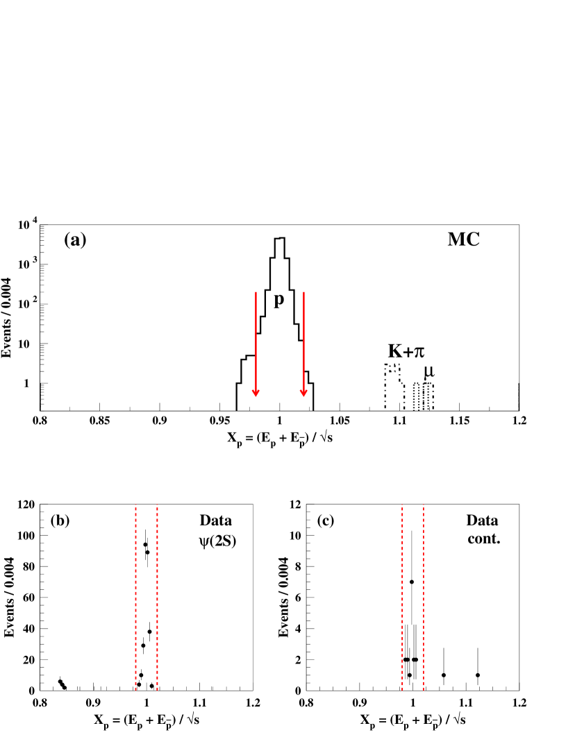
Figure 4.20: MC and data $X_{p}$ distributions for events which satisfy the $p\overline{p}$ final state event selection criteria. The arrows in Figure (a) and the dashed lines in Figures (b) and (c) denote the signal region of 0.98 $<$ $X_{p}$ $<$ 1.02. The solid histogram in Figure (a) is the $e^{+}e^{-}\rightarrow p\overline{p}$ signal MC obtained with $|G^{P}_{E}(s)|$ = 0 , the dashed histogram is Bhabha MC, the dotted histogram is dimuon MC, and the dot-dashed histogram is the $e^{+}e^{-}\rightarrow\pi^{+}\pi^{-}$ and $e^{+}e^{-}\rightarrow K^{+}K^{-}$ signal MC combined. Figure (b) is for the $\psi(2S)$ data sample. Figure (c) is for the continuum data sample. There are 269 events in the $\psi(2S)$ signal region and 16 events in the continuum signal region.

The same method is used for treating the $l^{+}l^{-}$ background as for the $K^{+}K^{-}$ final state analysis, as described at the end of Section 4.5.2. The peak region of $e^{+}e^{-}\rightarrow l^{+}l^{-}$ production for the $p\overline{p}$ analysis is 1.109 $<$ $X_{p}$ $<$ 1.155 and its corresponding leptonic MC scale factor is

$$\frac{N^{l^{+}l^{-}}_{MC}(0.98<X_{p}<1.02)}{N^{l^{+}l^{-}}_{MC}(1.109<X_{p}<1.155)}=\frac{1890\pm 43}{1,547,388\pm 1244}=(1.22\pm 0.03)\times 10^{-3}.$$

The number of events in the $l^{+}l^{-}$ peak region in both the $\psi(2S)$ and continuum data is found to be 1.00${}^{+1.75}_{-0.63}$, so the $l^{+}l^{-}$ background in the $p\overline{p}$ signal region is $N^{\psi(2S)}_{l^{+}l^{-}}=N^{cont}_{l^{+}l^{-}}=(1.22\pm 0.03)\times 10^{-3}$, and is considered negligible in the $p\overline{p}$ analysis.

4.6 Other Backgrounds

4.6.1 Contamination from Charmonium Resonances

Since the continuum data was taken at $\sqrt{s}$ = 3.671 GeV, contributions from nearby charmonium states need to be accounted for. The resonances considered are the off-mass shell production of the charmonium vector states J/$\psi$, $\psi(2S)$, $\psi(3770)$, $\psi(4040)$, $\psi(4160)$, and $\psi(4415)$, and the P-wave spin triplet states $\chi_{c0}$ and $\chi_{c2}$ produced via untagged two-photon fusion. Since the continuum data was only 15 MeV below the $\psi(2S)$ resonance, the contribution from the $\psi(2S)$ is treated directly in the Results section (Section 4.8). The resonance parameters of the listed charmonium states are given in Table 4.5.

Table 4.5: Charmonium resonances parameters. The full width, $e^{+}e^{-}$ partial width, and two-photon partial width are denoted by $\Gamma$, $\Gamma_{ee}$, and $\Gamma_{\gamma\gamma}$, respectively. The parameters for J/$\psi$, $\chi_{c0}$, $\chi_{c2}$, $\psi(2S)$, and $\psi(3770)$ are from the PDG [2]. The parameters for $\psi(4040)$, $\psi(4160)$, and $\psi(4415)$, are from Seth [196].

Resonance	Mass (GeV)	$\Gamma$ (MeV)	$\Gamma_{ee}$ (keV)	(2J+1)$\Gamma_{\gamma\gamma}$ (keV)
J/$\psi$	3.096916(11)	0.0910(32)	5.40(17)	—–
$\chi_{c0}$	3.41519(34)	10.1(8)	—–	2.6(5)
$\chi_{c2}$	3.55626(11)	2.11(16)	—–	2.6(3)
$\psi(2S)$	3.686093(34)	0.281(17)	2.12(12)	—–
$\psi(3770)$	3.7700(24)	23.6(2.7)	0.26(4)	—–
$\psi(4040)$	4.0394(9)	88(5)	0.89(8)	—–
$\psi(4160)$	4.153(3)	107(8)	0.83(7)	—–
$\psi(4415)$	4.426(5)	119(15)	0.71(10)	—–

Vector States, $\psi(nS)$

The contribution from the vector states are determined by convoluting a pure Born-level resonance with a Gaussian center-of-mass uncertainty inherent in $e^{+}e^{-}$ annihilations. The resonance production cross section of a vector state is characterized by a non-relativistic Breit-Wigner given as [2]

$$\sigma^{BW}_{V}(s)=\frac{3\pi}{s}\frac{\Gamma_{ee}\Gamma_{h\overline{h}}}{[(\sqrt{s}-M_{R})^{2}+(\Gamma/2)^{2}]},$$ (4.7)

where $s$ is the center-of-mass energy squared of the $e^{+}e^{-}$ annihilation, and $M_{R}$, $\Gamma$, $\Gamma_{ee}$, $\Gamma_{h\overline{h}}$ are the mass, full width, $e^{+}e^{-}$ partial width, and the $h\overline{h}$ $(\pi^{+},K^{+},$ or $p$) partial widths of the resonance. The $h\overline{h}$ partial widths of the J$/\psi$ and $\psi(2S)$ are listed in Table 4.6. None are known for the higher vectors. The distribution of the center-of-mass energy of the $e^{+}e^{-}$ annihilation is given by the following Gaussian expression

$$G(s,s^{\prime})=\frac{1}{\sqrt{2\pi}~{}\sigma_{CME}}~{}\exp\left(-\frac{(\sqrt{s}-\sqrt{s^{\prime}})^{2}}{2~{}\sigma^{2}_{CME}}\right),$$ (4.8)

where $s$ is the nominal center-of-mass energy squared, $s^{\prime}$ is the actual center-of-mass energy squared of the $e^{+}e^{-}$ annihilation, and $\sigma_{CME}=$ 2.3 MeV is the Gaussian uncertainty in the center-of-mass energy. The cross section of a resonance at the center-of-mass energy of the continuum data ($\sqrt{s}$ = 3.671 GeV) is given by the following convolution expression

$$\sigma_{V}(s)=\int^{\infty}_{0}\sigma^{BW}_{V}(s^{\prime})~{}G(s,s^{\prime})~{}d(s^{\prime}),$$ (4.9)

where $\sigma_{V}(s)$ is the observed cross section for $e^{+}e^{-}\rightarrow V\rightarrow h\overline{h}$.

Table 4.6: J/$\psi$ and $\psi(2S)$ partial widths for $\pi^{+}\pi^{-}$, $K^{+}K^{-}$, and $p\overline{p}$. The values are from the PDG [2].

Resonance	$\Gamma_{\pi^{+}\pi^{-}}$ (eV)	$\Gamma_{K^{+}K^{-}}$ (eV)	$\Gamma_{p\overline{p}}$ (eV)
J/$\psi$	13.4$\pm$2.1	21.6$\pm$2.9	193$\pm$11
$\psi(2S)$	22.5$\pm$14.1	28.1$\pm$19.7	58.2$\pm$9.4

The number of expected events in the continuum data sample, denoted by $N_{h\overline{h}}$, are determined by the expression

$$N_{h\overline{h}}=\sigma_{V}(s)\cdot\epsilon_{h\overline{h}}\cdot{\cal L},$$ (4.10)

where $\epsilon_{h\overline{h}}$ = 0.166, 0.743, and 0.657 for the $\pi^{+}\pi^{-}$, $K^{+}K^{-}$, and $p\overline{p}$ decays, respectively. Since the $h\overline{h}$ decay modes have not been experimentally observed for the $\psi(3770)$, $\psi(4040)$, $\psi(4160)$, and $\psi(4415)$ resonances, the J/$\psi$ partial widths for the corresponding final states have been used. Table 4.7 lists the number of $h\overline{h}$ events expected from the J/$\psi$, $\psi(3770)$, $\psi(4040)$, $\psi(4160)$, and $\psi(4415)$ resonances. The total number of $\pi^{+}\pi^{-}$, $K^{+}K^{-}$, $p\overline{p}$ events from charmonium vector states, excluding $\psi(2S)$, are (6.6$\pm$0.8)$\times 10^{-4}$, (4.9$\pm$0.6)$\times 10^{-3}$, and 0.039$\pm$0.003, respectively.

Table 4.7: Number of expected events from off-mass shell production of the J/$\psi$, $\psi(3770)$, $\psi(4040)$, $\psi(4160)$, and $\psi(4415)$ resonances.

Resonance	$N_{\pi^{+}\pi^{-}}$	$N_{K^{+}K^{-}}$	$N_{p\overline{p}}$
J/$\psi$	(20$\pm$3)$\times 10^{-5}$	(15$\pm$2)$\times 10^{-4}$	(117$\pm$7)$\times 10^{-4}$
$\psi(3770)$	(32$\pm$7)$\times 10^{-5}$	(24$\pm$5)$\times 10^{-4}$	(190$\pm$30)$\times 10^{-4}$
$\psi(4040)$	(7.9$\pm$1.4)$\times 10^{-5}$	(6.0$\pm$1.0)$\times 10^{-4}$	(46$\pm$5)$\times 10^{-4}$
$\psi(4160)$	(4.3$\pm$0.8)$\times 10^{-5}$	(3.3$\pm$0.5)$\times 10^{-4}$	(25.3$\pm$2.6)$\times 10^{-4}$
$\psi(4415)$	(1.5$\pm$0.3)$\times 10^{-5}$	(1.14$\pm$0.22)$\times 10^{-4}$	(8.9$\pm$1.3)$\times 10^{-4}$
Total	(6.6$\pm$0.8)$\times 10^{-4}$	(4.9$\pm$0.6)$\times 10^{-3}$	0.039$\pm$0.003

P-wave States, $\chi_{cJ}$

Untagged two-photon fusion resonance production occurs when a photon is emitted by each incident electron and positron, the two photons “fuse” to form the resonance, while the scattered electron and positron are not detected. Such two-photon events have some very distinct characteristics: the total observed energy is less than the center-of-mass energy of the two incident beams and, because the emitted photons are almost “real”, i.e., they have little transverse momentum, the transverse momentum of the produced resonance and hence its decay products is small. The resonance produced by the two “fused” photons has positive C parity and is observed by fully reconstructing its decay into a particular channel.

The total cross section for producing a resonance, $R$, in two-photon fusion is [187]

$$\sigma_{\gamma\gamma}(\sqrt{s},m_{R})=\frac{8\alpha^{2}(2J+1)\Gamma_{\gamma\gamma}(R)}{m^{3}_{R}}\left[\mathrm{f}\left(\frac{m^{2}_{R}}{s}\right)\left(\ln\frac{s}{m^{2}_{e}}-1\right)^{2}-\frac{1}{3}\left(\ln\frac{s}{m^{2}_{R}}\right)^{3}\right],$$

$$\mathrm{f}\left(\frac{m^{2}_{R}}{s}\right)=\left[\left(1+\frac{m^{2}_{R}}{2s}\right)^{2}\ln\frac{s}{m^{2}_{R}}\right]-\left[\frac{1}{2}\left(1-\frac{m^{2}_{R}}{s}\right)\left(3+\frac{m^{2}_{R}}{s}\right)\right]$$ (4.11)

where $J$, $m_{R}$, and $\Gamma_{\gamma\gamma}(R)$ is the total angular momentum, mass, and two-photon partial width of the produced resonance, respectively.

The number of expected events in the continuum data sample are determined by the expression

$$N_{h\overline{h}}=\sigma_{\gamma\gamma}(\sqrt{s},m_{R})\cdot\epsilon_{h\overline{h}}\cdot{\cal L}\cdot{\cal B}(\chi_{c0,2}\rightarrow h\overline{h}),$$ (4.12)

where $\epsilon_{h\overline{h}}$ are 0.166, 0.743, and 0.657 for the $\pi^{+}\pi^{-}$, $K^{+}K^{-}$, and $p\overline{p}$ decays, respectively. By using the same efficiencies as for the direct production of the $h\overline{h}$ final states, a conservative estimate of the number of events is determined since the efficiency should be lower due to the net momentum and signal region selection criteria. As is apparent in Figures 4.8a and 4.13a, the $h\overline{h}$ final states from $\chi_{c0}$ and $\chi_{c2}$ will peak in their respective $X_{\pi,K}$ at 0.926 and 0.965, respectively. The branching ratios ${\cal B}(\chi_{c0,2}\rightarrow h\overline{h})$ are given in Table 4.8. Table 4.9 lists the results of the number of $h\overline{h}$ events expected from the $\chi_{c0}$ and $\chi_{c2}$ produced in untagged two-photon fusion. Under the assumption that all events from the decays of the $\chi_{c0}$ and $\chi_{c2}$ were to populate the corresponding signal regions, the total number of $\pi^{+}\pi^{-}$, $K^{+}K^{-}$, and $p\overline{p}$ events from $\chi_{c0}$ and $\chi_{c2}$ decays produced in untagged two-photon fusion are (2.2$\pm$0.4)$\times 10^{-3}$, 0.011$\pm$0.003, and (3.7$\pm$0.8)$\times 10^{-4}$, respectively.

The total number of background events from neighboring charmonium states, except from $\psi(2S)$, i.e., the sum of the totals in Tables 4.7 and 4.9, are (2.9$\pm$0.6)$\times 10^{-3}$, 0.016$\pm$0.003, and 0.038$\pm$0.009 for the $\pi^{+}\pi^{-}$, $K^{+}K^{-}$, and $p\overline{p}$ final states, respectively, These values are considered negligible for the determination of the electromagnetic form factors. The $\psi(2S)$ decays to the $h\overline{h}$ final states are specifically treated in the Results section (Section 4.8).

Table 4.8: $\chi_{c0}$ and $\chi_{c2}$ branching ratios for $\pi^{+}\pi^{-}$, $K^{+}K^{-}$, and $p\overline{p}$. The values are from the PDG [2].

Resonance	${\cal B}(R\rightarrow\pi^{+}\pi^{-})$	${\cal B}(R\rightarrow K^{+}K^{-})$	${\cal B}(R\rightarrow p\overline{p})$
$\chi_{c0}$	(4.9$\pm$0.5)$\times 10^{-3}$	(6.0$\pm$0.9)$\times 10^{-3}$	(2.24$\pm$0.27)$\times 10^{-4}$
$\chi_{c2}$	(1.77$\pm$0.27)$\times 10^{-3}$	(9.4$\pm$2.1)$\times 10^{-4}$	(6.8$\pm$0.7)$\times 10^{-5}$

Table 4.9: Number of expected events from untagged two-photon fusion production of the $\chi_{c0}$ and $\chi_{c2}$ resonances.

Resonance	$N_{\pi^{+}\pi^{-}}$	$N_{K^{+}K^{-}}$	$N_{p\overline{p}}$
$\chi_{c0}$	(19$\pm$4)$\times 10^{-4}$	(100$\pm$30)$\times 10^{-4}$	(33$\pm$8)$\times 10^{-5}$
$\chi_{c2}$	(2.6$\pm$0.5)$\times 10^{-4}$	(6.2$\pm$1.6)$\times 10^{-4}$	(4.0$\pm$0.6)$\times 10^{-5}$
Total	(2.2$\pm$0.4)$\times 10^{-3}$	0.011$\pm$0.003	(3.7$\pm$0.8)$\times 10^{-4}$

4.6.2 Common Collider Backgrounds

Two types of backgrounds are common to all collider experiments. The first type of background is related to unwanted beam collisions with the residual gas in the beam pipe (called beam-gas) and with the beam pipe wall (beam-wall). The other type of background is due to cosmic rays, typically muons, traversing the detector. These backgrounds sources are observed in the IP variables $d_{b}$ and $z_{b}$ (see Section 4.4 for the definitions of $d_{b}$ and $z_{b}$) and the track variable $\phi_{0}$. The variable $\phi_{0}$ is the azimuthal angle of the track defined in the plane perpendicular to the positron beam (or $z$-axis) and with respect to the $x$-axis, which points radially outward from the storage ring.

Figure 4.21 shows the $\phi_{0}$ distribution for positive tracks in continuum data events. A cosmic ray typically traverses the detector in the vertical (or $y$) direction. This is apparent by the abundance of events at $\phi_{0}$ = $\pi/2$ = 1.57 radians (up) and $\phi_{0}$ = $3\pi/2$ = 4.71 radians (down). A majority of the cosmic ray events is removed by the IP and track quality criteria (dashed histogram).

Figure 4.22 shows the two-dimensional distribution of the IP variables $d_{b}$ and $z_{b}$ for events in the continuum data sample which pass the acceptance and trigger criteria. The background events surrounding the volume defined by the nominal IP region, $|d_{b}|$ $<$ 5 mm and $|z_{b}|$ $<$ 5 cm, are analyzed to test for possible contamination. This background volume, which is arbitrarily taken to be twice as large as the nominal IP region, is bounded by $|d_{b}|$ $<$ 7.2 mm and $|z_{b}|$ $<$ 7.2 cm, while excluding the volume defined by the nominal IP region. After applying the respective $h\overline{h}$ final state criteria, no events are found in the corresponding $X_{h}$ signal regions originating from this sideband volume. Based on these studies, possible contamination from beam-gas, beam-wall, and cosmic ray backgrounds are considered negligible.

Figure 4.21: Azimuthal angle ($\phi_{0}$) distribution of positive tracks in the continuum data sample. The dotted histogram are events which satisfy the acceptance (Acc) and trigger (Trig) criteria. The dashed histogram are events which satisfy the acceptance, trigger, IP, and track quality (TQ) criteria. The solid histogram are events in the $X_{\pi}$ signal region (0.98 $<$ $X_{p}$ $<$ 1.02) which satisfy the acceptance, trigger, IP, and track quality criteria. Similar features are present in the $X_{K}$ and $X_{p}$ signal regions.

Figure 4.22: Two-dimensional distribution of the IP variables $d_{b}$ and $z_{b}$ in the continuum data sample. Only the acceptance and trigger selection criteria have been applied. The IP selection criteria accepts events if the tracks have $|d_{b}|$ $<$ 5 mm and $|z_{b}|$ $<$ 5 cm, as shown by the box. The outer boundary of the figure corresponds to a total volume which is three times larger than is enclosed by the inner box.

4.7 Radiative Corrections

The effect of initial state radiative corrections to the production of a virtual photon in $e^{+}e^{-}$ annihilation needs to be determined to obtain the Born cross section for $e^{+}e^{-}\rightarrow h\overline{h}$ $(h=\pi^{+},K^{+},p)$ from the experimentally measured cross section. Figure 4.23 (top) shows the Born, or tree-level, Feynman diagram for hadron pair production. Figure 4.23 also shows the Feynman diagrams for radiative corrections corresponding to the $e^{+}e^{-}$ annihilation vertex correction, vacuum polarization of the virtual photon, and bremstrahlung radiation from the colliding $e^{+}e^{-}$ pair.

Figure 4.23: Feynman diagrams associated with $e^{+}e^{-}\rightarrow h\overline{h}$. The top figure is the Born, or tree-level, diagram. The middle left figure is the $e^{+}e^{-}$ annihilation vertex correction, the middle right figure is the vacuum polarization correction from lepton pair loops, and the bottom figures are the initial state radiation bremstrahlung corrections.

The radiative corrections are determined using the method of Bonneau and Martin [188], with the addition of $\mu$ and $\tau$ pair loops to the vacuum polarization correction. This is also the first method suggested by Berends and Kleiss [189]. The Born cross section, $\sigma_{0}(s)$, is related to the experimental cross section, $\sigma_{exp}(s)$, by

$$\sigma_{0}(s)=\frac{\sigma_{exp}(s)}{(1+\delta)}$$ (4.13)

where $s$ is the center-of-mass energy squared of the initial $e^{+}e^{-}$ system and $\delta$ is the radiative correction. The radiative correction is expressed as [188]

$$\delta=\frac{2\alpha}{\pi}\left(\frac{3}{4}~{}\mathrm{ln}\frac{s}{m^{2}_{e}}+\frac{\pi^{2}}{6}-1\right)~{}+\sum_{l=e,\mu,\tau}\frac{2\alpha}{\pi}\left(\frac{1}{3}~{}\mathrm{ln}\frac{s}{m^{2}_{l}}-\frac{5}{9}\right)~{}+~{}t(\mathrm{ln}x_{min})$$

$$+~{}t\left[~{}\int^{x_{max}}_{x_{min}}\frac{dx}{x}\left(1-x+\frac{x^{2}}{2}\right)\frac{\sigma_{0}(s(1-x))}{\sigma_{0}(s)}\frac{\epsilon(x)}{\epsilon(0)}~{}\right],$$ (4.14)

where $\alpha$ is the fine-structure constant, $m_{e}$ is the electron mass, $x$ is the ratio of the bremstrahlung photon energy to the beam energy defined as $x$ = $E_{\gamma}/E_{b}$, $\epsilon(x)$ is the experimental detection efficiency as a function of $x$, and

$$t=\frac{2\alpha}{\pi}\left(\mathrm{ln}\frac{s}{m^{2}_{e}}-1\right).$$ (4.15)

The first term in Eq. 4.14 is the vertex correction, the second term is the sum of the leptonic loop contributions to the vacuum polarization correction, and the last two terms are associated with bremstrahlung radiation from the colliding $e^{+}e^{-}$ pair. Since the integral in the last term is infrared divergent, the third term corresponds to the low energy cutoff of the bremstrahlung integral. In order to evaluate the bremstrahlung integral, the efficiency ratio $\epsilon(x)/\epsilon(0)$ is determined from initial state radiation (ISR) MC samples and the cross section ratio $\sigma_{0}(s(1-x))/\sigma_{0}(s)$ is described in the following paragraphs.

As already mentioned in Eqn. 1.15, the differential cross section for $e^{+}e^{-}\rightarrow m^{+}m^{-}$ ($m$ = $\pi,K$) can be expressed as [13]

$$\frac{d\sigma_{0}(s)}{d\Omega}=\frac{\alpha^{2}}{8s}~{}\beta^{3}_{m}~{}|F_{m}(s)|^{2}~{}\mathrm{sin}^{2}\theta,$$ (4.16)

where $\beta_{m}$ and $F_{m}(s)$ is the pseudoscalar meson velocity (in terms of c) measured in the laboratory system and electromagnetic form factor, respectively. Integrating over $\theta$, the total cross section is

$$\sigma_{0}(s)=\frac{\pi\alpha^{2}}{3s}~{}\beta^{3}_{m}~{}|F_{m}(s)|^{2}.$$ (4.17)

The cross section ratio for $e^{+}e^{-}\rightarrow m^{+}m^{-}$, using $\beta_{m}$ = $\sqrt{1-(4m^{2}_{m}/s)}$, where $m_{m}$ is the mass of the meson, and making the PQCD assumption that $|F_{m}(s)|\propto s^{-1}$, is

$$\frac{\sigma_{0}(s(1-x))}{\sigma_{0}(s)}=\frac{1}{(1-x)^{9/2}}~{}\left[\frac{s(1-x)-4m^{2}_{m}}{s-4m^{2}_{m}}\right]^{3/2}.$$ (4.18)

As already mentioned in Eqn. 1.13, the differential cross section for $e^{+}e^{-}\rightarrow p\overline{p}$ can be expressed as

$$\frac{d\sigma_{0}(s)}{d\Omega}=\frac{\alpha^{2}}{4s}\beta_{p}\left[|G^{P}_{M}(s)|^{2}~{}(1+\mathrm{cos}^{2}\theta)+\left(\frac{4m^{2}_{p}}{s}\right)|G^{P}_{E}(s)|^{2}~{}(\mathrm{sin}^{2}\theta)\right].$$ (4.19)

Integrating over $\theta$, the total cross section is

$$\sigma_{0}(s)=\frac{4\pi\alpha^{2}}{3s}\beta_{p}~{}|G^{P}_{M}(s)|^{2}~{}\left(1+\frac{2m^{2}_{p}}{s}\cdot r\right),$$ (4.20)

where $r=|G^{P}_{E}(s)|^{2}/|G^{P}_{M}(s)|^{2}$. The cross section ratio $\sigma_{0}(s(1-x))/\sigma_{0}(s)$ for $e^{+}e^{-}\rightarrow p\overline{p}$, using $\beta_{p}$ = $\sqrt{1-(4m^{2}_{p}/s)}$ and making the PQCD assumption that $|G^{P}_{M}(s)|\propto s^{-2}$, is

$$\frac{\sigma_{0}(s(1-x))}{\sigma_{0}(s)}=\frac{1}{(1-x)^{13/2}}~{}\left[\frac{s(1-x)-4m^{2}_{p}}{s-4m^{2}_{p}}\right]^{1/2}~{}\left[\frac{s(1-x)-2m^{2}_{p}\cdot r}{s-2m^{2}_{p}\cdot r}\right].$$ (4.21)

The efficiency ratio $\epsilon(x)/\epsilon(0)$ is determined by generating ISR MC samples for a particular final state as a function of bremstrahlung photon energy, $E_{\gamma}$. The ISR MC starts at the continuum center-of-mass energy and goes to a generic delta-function “resonance” and a single ISR photon. This makes the reaction a two-body decay followed by the “resonance” decaying to the final state of interest.

The ISR MC sample consists of individual subsamples with $E_{\gamma}$ fixed, starting with $E_{\gamma}$ = 10 keV, and each subsequent subsample with $E_{\gamma}$ increasing by 2 MeV. There are 10,000 generated events in each individual sample. The value of $\epsilon(0)$, the efficiency with no ISR, is determined from a 10,000 event MC sample generated with the initial center-of-mass energy fixed at $\sqrt{s}$ = 3.671 GeV. Note that all MC samples have final state radiation incorporated.

Figures 4.24a, 4.24b, and 4.24c (top row) show $\epsilon(x)/\epsilon(0)$ as a function of $x$ for the $\pi^{+}\pi^{-}$, $K^{+}K^{-}$, and $p\overline{p}$ final states, respectively. The detection efficiency drops to zero around $x$ = 0.05 ($E_{\gamma}$ = 92 MeV). Figures 4.24d, 4.24e, and 4.24f (bottom) show how the numerically-evaluated bremstrahlung integral in Eqn. 4.14 varies as a function of $x$.

Figure 4.24: Efficiency ratio (top row) and bremstrahlung integral (bottom row) distributions. The left, middle, and right columns are for the $\pi^{+}\pi^{-}$, $K^{+}K^{-}$, and $p\overline{p}$ final states, respectively. The bremstrahlung variable $B(x)$ is defined by Eqn. 4.22.

The radiative correction at $\sqrt{s}$ = 3.671 GeV, with a bremstrahlung energy cutoff of $E_{\gamma,min}$ = 10 keV ($x_{min}$ = $5.448\times 10^{-6}$), is

$$1+\delta=1+(0.0649)+(0.0330)+t(-12.1202)+t\Sigma B(x)\Delta x=0.154+t\Sigma B(x)\Delta x.$$

where $t$ = 0.0779 and

$$B(x)=\frac{1}{x}\left(1-x+\frac{x^{2}}{2}\right)\frac{\sigma_{0}(s(1-x))}{\sigma_{0}(s)}\frac{\epsilon(x)}{\epsilon(0)}.$$ (4.22)

The radiative corrections to $\sigma_{0}(e^{+}e^{-}\rightarrow\pi^{+}\pi^{-})$, $\sigma_{0}(e^{+}e^{-}\rightarrow K^{+}K^{-})$, and $\sigma_{0}(e^{+}e^{-}\rightarrow p\overline{p})$ are listed is Table 4.10. The radiative corrections have the effect of increasing the experimental cross sections by 14-19$\%$.

Table 4.10: Radiative corrections for $\sigma_{0}(e^{+}e^{-}\rightarrow\pi^{+}\pi^{-})$, $\sigma_{0}(e^{+}e^{-}\rightarrow K^{+}K^{-})$, and $\sigma_{0}(e^{+}e^{-}\rightarrow p\overline{p})$ at $\sqrt{s}$ = 3.671 GeV. The variable $B(x)$ is defined by Eqn. 4.22.

Final State	$\Sigma B(x)\Delta x$	$1+\delta$
$\pi^{+}\pi^{-}$	8.692	0.831
$K^{+}K^{-}$	8.426	0.810
$p\overline{p}$	8.969	0.853
$(|G^{P}_{E}(s)|=0)$
$p\overline{p}$	9.057	0.860
$(|G^{P}_{E}(s)|=|G^{P}_{M}(s)|)$

4.8 Results for the Form Factors

In this presentation we use the following convention to specify the number of counts, $N$. The $\underline{\mathrm{superscripts}}$ ’$\psi(2S)$’ and ’cont’ denote the source of the data: the $\psi(2S)$ and continuum data samples. The $\underline{\mathrm{subscripts}}$ ’obs’, ’$l^{+}l^{-}$’, ’$\psi(2S)$’, and ’cont’ denote the observed counts, and the contamination counts: the $l^{+}l^{-}$ background, the $\psi(2S)$, and the continuum contributions, respectively.

4.8.1 Determination of ${\cal B}(\psi(2S)\rightarrow h\overline{h})$

Form factor measurements are made at energies removed from resonances which can be formed or decay into $e^{+}e^{-}$, such as J$/\psi$ or $\psi(2S)$. However, studying the decays of $\psi(2S)\rightarrow h\overline{h}$ ($h$ = $\pi^{+},K^{+},p$) serve two important purposes: they can be used to cross check the analysis procedure for measuring the form factors, and they are necessary for determining the amount of $\psi(2S)$ tail in the continuum data sample for a given final state.

The branching ratio for $\psi(2S)\rightarrow h\overline{h}$ is determined by

$${\cal{B}}(\psi(2S)\rightarrow h\overline{h})=\frac{N(\psi(2S)\rightarrow h\overline{h})}{\epsilon_{h}N^{\psi(2S)}_{prod}},$$ (4.23)

where the number of $\psi(2S)\rightarrow h\overline{h}$ signal events is

$$N(\psi(2S)\rightarrow h\overline{h})=N^{\psi(2S)}_{obs}-N^{\psi(2S)}_{l^{+}l^{-}}-N^{\psi(2S)}_{cont},$$ (4.24)

and $N^{\psi(2S)}_{obs}$ is the number of observed events, $N^{\psi(2S)}_{l^{+}l^{-}}$ is the expected number of $l^{+}l^{-}$ background events, and $N^{\psi(2S)}_{cont}$ is the number of $e^{+}e^{-}\rightarrow h\overline{h}$ events, all for the $\psi(2S)$ data sample. The $h\overline{h}$ final state detection efficiency is denoted by $\epsilon_{h}$ and $N^{\psi(2S)}_{prod}$ = 1.52$\times 10^{6}$ is the total number of $\psi(2S)$ events in the $\psi(2S)$ data sample [183]. The number of $e^{+}e^{-}\rightarrow h\overline{h}$ events in the $\psi(2S)$ data sample from the continuum contribution is

$$N^{\psi(2S)}_{cont}=A_{n}\left(N^{cont}_{obs}-N^{cont}_{l^{+}l^{-}}-N^{cont}_{\psi(2S)}\right),$$ (4.25)

where $N^{cont}_{obs}$ is the number of observed events, $N^{cont}_{l^{+}l^{-}}$ is the expected number of $l^{+}l^{-}$ background events, and $N^{cont}_{\psi(2S)}$ is the number of $\psi(2S)$ events, all for the continuum data sample. The quantity $A_{n}$ in Eqn. 4.25 is the continuum scaling factor. It is defined as

$$A_{n}=({\cal{L}}_{\psi(2S)}/{\cal{L}}_{cont})\cdot(s_{cont}/s_{\psi(2S)})^{n},$$ (4.26)

where $n$ denotes the inverse s-dependence of the $e^{+}e^{-}\rightarrow h\overline{h}$ cross section, i.e., for $\pi^{+}\pi^{-}$ and $K^{+}K^{-}$, $n$ = 3 ($\sigma_{0}(s)\propto s^{-3}$) gives $A_{3}$ = 0.136, and for $p\overline{p}$, $n$ = 5 ($\sigma_{0}(s)\propto s^{-5}$) gives $A_{5}$ = 0.134.

In turn, the number of $\psi(2S)$ events in the continuum data is defined as

$$N^{cont}_{\psi(2S)}=C^{\pi^{+}\pi^{-}J/\psi}(N^{\psi(2S)}_{obs}-N^{\psi(2S)}_{l^{+}l^{-}}),$$ (4.27)

where $N^{\psi(2S)}_{obs}$ and $N^{\psi(2S)}_{l^{+}l^{-}}$ are the number of observed events and the expected number of $l^{+}l^{-}$ background events in the $\psi(2S)$ data sample, respectively. The scale factor $C^{\pi^{+}\pi^{-}J/\psi}$ = 0.0072$\pm$0.0005 is the contamination from $\psi(2S)$ in the continuum data, as defined in Eqn. 4.1. At this level, the continuum content of the $\psi(2S)$ data itself is considered negligible.

4.8.2 Determination of $\sigma_{0}(e^{+}e^{-}\rightarrow h\overline{h})$

The Born cross section for $e^{+}e^{-}\rightarrow h\overline{h}$ for the continuum data is determined by

$$\sigma_{0}(e^{+}e^{-}\rightarrow h\overline{h})=\frac{N^{cont}(e^{+}e^{-}\rightarrow h\overline{h})}{\epsilon_{h}(1+\delta){\cal{L}}_{cont}},$$ (4.28)

where the number of $e^{+}e^{-}\rightarrow h\overline{h}$ signal events is

$$N^{cont}(e^{+}e^{-}\rightarrow h\overline{h})=N^{cont}_{obs}-N^{cont}_{l^{+}l^{-}}-N^{cont}_{\psi(2S)},$$ (4.29)

and $N^{cont}_{obs}$ is the number of observed events, $N^{cont}_{l^{+}l^{-}}$ is the expected number of $l^{+}l^{-}$ background events, and $N^{cont}_{\psi(2S)}$ is the number of $\psi(2S)$ contamination events, all for the continuum data sample. The $h\overline{h}$ final state detection efficiency and radiative correction are denoted by $\epsilon_{h}$ and $1+\delta$, respectively, while ${\cal{L}}_{cont}$ = 20.7 pb^-1 is the integrated luminosity for the continuum data sample. The radiative corrections are listed in Table 4.10. The number of $\psi(2S)\rightarrow h\overline{h}$ events in the continuum data is

$$N^{cont}_{\psi(2S)}=C^{\pi^{+}\pi^{-}J/\psi}(N^{\psi(2S)}_{obs}-N^{\psi(2S)}_{l^{+}l^{-}}-N^{\psi(2S)}_{cont}),$$ (4.30)

where $N^{\psi(2S)}_{obs}$ is the number of observed events, $N^{\psi(2S)}_{l^{+}l^{-}}$ is the expected number of $l^{+}l^{-}$ background events, and $N^{\psi(2S)}_{cont}$ is the number of $e^{+}e^{-}\rightarrow h\overline{h}$ events, all for the $\psi(2S)$ data sample. The scale factor $C^{\pi^{+}\pi^{-}J/\psi}$ is the $\psi(2S)$ contamination in the continuum data, as defined in Eqn. 4.1. The number of $e^{+}e^{-}\rightarrow h\overline{h}$ events in the $\psi(2S)$ data is defined as

$$N^{\psi(2S)}_{cont}=A_{n}\left(N^{cont}_{obs}-N^{cont}_{l^{+}l^{-}}\right),$$ (4.31)

where $N^{cont}_{obs}$ and $N^{cont}_{l^{+}l^{-}}$ are the number of observed events and the expected number of $l^{+}l^{-}$ background events in the continuum data sample, respectively. The quantity $A_{n}$ is the continuum scaling factor, as defined in Eqn. 4.26. At this level, the $\psi(2S)$ content in the continuum data itself is considered negligible.

4.8.3 Determination of ${\cal B}(\psi(2S)\rightarrow\pi^{+}\pi^{-})$

Figure 4.10 shows both the $X_{\pi}$ signal region and its vicinity after the $\pi^{+}\pi^{-}$ event selection criteria have been applied to the $\psi(2S)$ and continuum data samples. There are 8 events in the $X_{\pi}$ signal region for the $\psi(2S)$ data sample and 26 events for the continuum data sample. Figure 4.25 shows that the $\psi(2S)$ data events are confined to the regions predicted by the signal MC.

Figure 4.25: The $\psi(2S)$ data with the $\pi^{+}\pi^{-}$ final state criteria applied. The points are data events. The solid histograms are $e^{+}e^{-}\rightarrow\pi^{+}\pi^{-}$ signal MC, normalized to the number of observed events in the signal region. Figure (a): $X_{\pi}$ distribution. The $X_{\pi}$ signal region is enclosed by the dashed lines. The points near $X_{\pi}$ = 0.85 are associated with $\psi(2S)\rightarrow p\overline{p}$ decays. Figure (b): $X_{\pi}$ signal region. The dashed histogram is the continuum data scaled according to Eqn. 4.26. Figure (c): $\Delta\chi^{2}(\pi-e)$ for the positive track. Figure (d): $E_{tkCC}$ for the positive track. Figure (e): Net momentum of the two tracks. Figure (f): $|$cos($\theta$)$|$ for the positive track.

The number of $e^{+}e^{-}\rightarrow\pi^{+}\pi^{-}$ events in the $\psi(2S)$ data sample is

$$N^{\psi(2S)}_{cont}=A_{3}[(26.0\pm 5.1)-(0.108\pm 0.013)-(0.057\pm 0.024)]=3.5\pm 0.7.$$

The number of $\psi(2S)\rightarrow\pi^{+}\pi^{-}$ signal events is

$$N(\psi(2S)\rightarrow h\overline{h})=(8.0^{+3.3}_{-2.7})-(3.5\pm 0.7)-(0.021\pm 0.002)=4.5^{+3.4}_{-2.8}$$

From Eqn. 4.23, the $\psi(2S)\rightarrow\pi^{+}\pi^{-}$ branching ratio is

$${\cal{B}}(\psi(2S)\rightarrow\pi^{+}\pi^{-})=\frac{N(\psi(2S)\rightarrow\pi^{+}\pi^{-})}{\epsilon_{h}N^{\psi(2S)}_{prod}}~{}~{}~{}~{}~{}~{}~{}~{}~{}~{}~{}~{}~{}~{}~{}~{}~{}~{}~{}~{}~{}~{}~{}~{}~{}~{}~{}~{}~{}~{}~{}~{}~{}~{}~{}~{}~{}~{}~{}~{}~{}~{}~{}~{}~{}~{}~{}~{}~{}~{}~{}$$

$$=\frac{4.5^{+3.4}_{-2.8}}{(0.166)(1.52\times 10^{6})}=(1.8^{+1.3}_{-1.1}(stat))\times 10^{-5}.$$

This value of ${\cal{B}}(\psi(2S)\rightarrow\pi^{+}\pi^{-})$ is a factor $\sim$4 smaller than the PDG value of ${\cal{B}}(\psi(2S)\rightarrow\pi^{+}\pi^{-})$ = $(8\pm 5)\times 10^{-5}$ [2], but consistent with the recent BES I measurement of ${\cal{B}}(\psi(2S)\rightarrow\pi^{+}\pi^{-})$ = $(0.84\pm 0.55^{+0.16}_{-0.35})\times 10^{-5}$ [197]. Our result is also only 1.6$\sigma$ above a null observation.

4.8.4 Determination of $\sigma(e^{+}e^{-}\rightarrow\pi^{+}\pi^{-})$ and $|F_{\pi}(s)|$

Figure 4.26 shows the event distributions for several variables for the continuum data and signal MC after applying the $\pi^{+}\pi^{-}$ event selection criteria. There are 26 observed events in the $\pi^{+}\pi^{-}$ signal region. The data events are distributed in accord with the signal MC predictions.

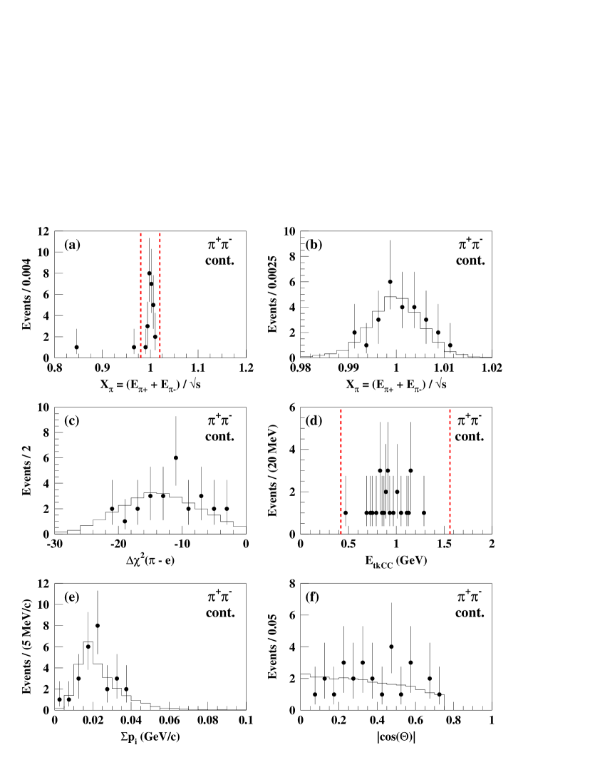
Figure 4.26: Continuum data sample with the $\pi^{+}\pi^{-}$ final state criteria applied. The points are data events. The solid histogram are $e^{+}e^{-}\rightarrow\pi^{+}\pi^{-}$ signal MC, normalized to the number of observed events in the signal region. Figure (a): $X_{\pi}$ distribution. The $X_{\pi}$ signal region is enclosed by the dashed lines. Figure (b): $X_{\pi}$ signal region. Figure (c): $\Delta\chi^{2}(\pi-e)$ for the positive track. Figure (d): $E_{tkCC}$ for the positive track. Figure (e): Net momentum of the two tracks. Figure (f): $|$cos($\theta$)$|$ for the positive track.

The values of all measured quantities for the 26 observed events are listed in Tables A.1-10 of Appendix A. Two interesting features are present. Table A.7 lists the $dE/dx$+RICH PID variable $\Delta\chi^{2}(\pi-\mu)$, and it is apparent that it does not contain discriminating power between pions and muons. As seen in Table A.10, one pion candidate track has an associated signal in the muon detector. A pion track will decay to a muon $\sim$3$\%$ of the time according to the $e^{+}e^{-}\rightarrow\pi^{+}\pi^{-}$ signal MC. Therefore, one pion decaying to a muon, out of 52 candidates, is consistent with the MC prediction.

The number of $\psi(2S)\rightarrow\pi^{+}\pi^{-}$ events in the continuum data sample is

$$N^{cont}_{\psi(2S)}=C^{\pi^{+}\pi^{-}J/\psi}[(8.0^{3.3}_{2.7})-(0.021\pm 0.002)-(3.5\pm 0.7)]=0.03\pm 0.02.$$

The number of $e^{+}e^{-}\rightarrow\pi^{+}\pi^{-}$ signal events is

$$N^{cont}(e^{+}e^{-}\rightarrow\pi^{+}\pi^{-})=(26.0\pm 5.1)-(0.108\pm 0.013)-(0.03\pm 0.02)=25.9\pm 5.1.$$

Therefore, using Eqn. 4.28, the cross section for $e^{+}e^{-}\rightarrow\pi^{+}\pi^{-}$ is

$$\sigma_{0}(e^{+}e^{-}\rightarrow\pi^{+}\pi^{-})=\frac{N^{cont}(e^{+}e^{-}\rightarrow\pi^{+}\pi^{-})}{\epsilon_{h}(1+\delta){\cal{L}}_{cont}}~{}~{}~{}~{}~{}~{}~{}~{}~{}~{}~{}~{}~{}~{}~{}~{}~{}~{}~{}~{}~{}~{}~{}~{}~{}~{}~{}~{}~{}~{}~{}~{}~{}~{}~{}~{}~{}~{}~{}~{}~{}~{}~{}~{}~{}~{}~{}~{}~{}~{}~{}$$

$$=\frac{25.9\pm 5.1}{(0.166)(0.832)(20.7~{}\mathrm{pb^{-1}})}=9.0\pm 1.8~{}\mathrm{pb}.$$

As stated in Eqn. 1.15, the cross section is related to the pion electromagnetic form factor by [13]

$$\sigma_{0}(e^{+}e^{-}\rightarrow\pi^{+}\pi^{-})=\frac{\pi\alpha^{2}\beta^{3}_{\pi}}{3s}|F_{\pi}(s)|^{2}.$$ (4.32)

Inserting the constants in the equation above, the pion form factor at $\sqrt{s}$ = 3.671 GeV is

$$|F_{\pi}(13.48~{}\mathrm{GeV}^{2})|=\sqrt{\frac{9.0\pm 1.8~{}\mathrm{pb}}{1598~{}\mathrm{pb}}}=0.075\pm 0.008$$ (4.33)

where the errors are statistical only.

4.8.5 Determination of ${\cal B}(\psi(2S)\rightarrow K^{+}K^{-})$

Figure 4.15 shows both the $X_{K}$ signal region and its vicinity after the $K^{+}K^{-}$ event selection criteria have been applied to the $\psi(2S)$ and continuum data sample. There are 92 events in the $X_{K}$ signal region for the $\psi(2S)$ data sample and 72 events for the continuum data sample. Figure 4.27 shows that the distributions of the $\psi(2S)$ data events are in agreement with the $e^{+}e^{-}\rightarrow K^{+}K^{-}$ signal MC predictions.

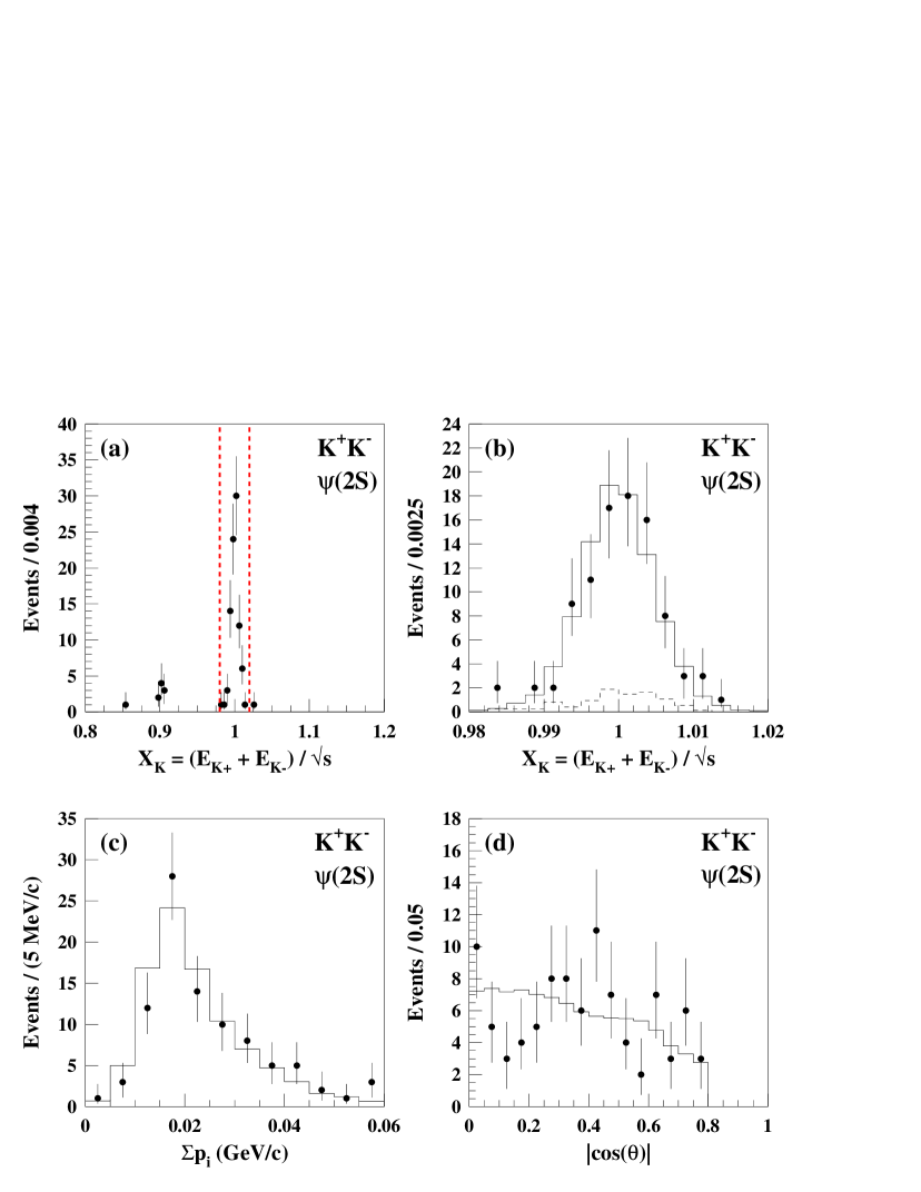
Figure 4.27: The $\psi(2S)$ data with the $K^{+}K^{-}$ final state criteria applied. The points are data events. The solid histograms are the $e^{+}e^{-}\rightarrow K^{+}K^{-}$ signal MC, normalized to the number of observed events in the signal region. Figure (a): $X_{K}$ distribution. The $X_{K}$ signal region is enclosed by the dashed lines. The points near $X_{K}$ = 0.90 are associated with $\psi(2S)\rightarrow p\overline{p}$ decays. Figure (b): $X_{K}$ signal region. The dashed histogram is the continuum data scaled according to Eqn. 4.26. Figure (c): Net momentum of the two tracks. Figure (d): $|$cos($\theta$)$|$ for the positive track.

The number of $e^{+}e^{-}\rightarrow K^{+}K^{-}$ events in the $\psi(2S)$ data sample is

$$N^{\psi(2S)}_{cont}=A_{3}[(72.0\pm 8.5)-(0.56^{+0.21}_{-0.18})-(0.66\pm 0.08)]=9.6\pm 1.2.$$

The number of $\psi(2S)\rightarrow K^{+}K^{-}$ signal events is

$$N(\psi(2S)\rightarrow K^{+}K^{-})=(92.0\pm 9.6)-(0.06^{+0.10}_{-0.04})-(9.6\pm 1.2)=82.3\pm 9.7.$$

From Eqn. 4.23, the $\psi(2S)\rightarrow K^{+}K^{-}$ branching ratio is

$${\cal{B}}(\psi(2S)\rightarrow K^{+}K^{-})=\frac{82.3\pm 9.7}{(0.743)(1.52\times 10^{6})}=(7.3\pm 0.9(stat))\times 10^{-5}.$$

This value of ${\cal{B}}(\psi(2S)\rightarrow K^{+}K^{-})$ is consistent with the PDG value of ${\cal{B}}(\psi(2S)\rightarrow K^{+}K^{-})$ = $(10\pm 7)\times 10^{-5}$ [2] and the BES I measurement of ${\cal{B}}(\psi(2S)\rightarrow K^{+}K^{-})$ = $(6.1\pm 1.4^{+1.5}_{-1.3})\times 10^{-5}$ [197].

4.8.6 Determination of $\sigma(e^{+}e^{-}\rightarrow K^{+}K^{-})$ and $|F_{K}(s)|$

Figure 4.28 shows the event distributions for several variables for the continuum data and signal MC after applying the $K^{+}K^{-}$ event selection criteria. There are 72 observed events in the $K^{+}K^{-}$ signal region. The distributions of data events are in agreement with the signal MC predictions.

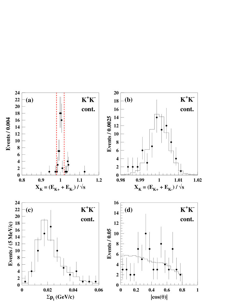
Figure 4.28: Continuum data sample with the $K^{+}K^{-}$ final state criteria applied. The points are data events. The solid histograms are $e^{+}e^{-}\rightarrow K^{+}K^{-}$ signal MC, normalized to the number of observed events in the signal region. Figure (a): $X_{K}$ distribution. The $X_{K}$ signal region is enclosed by the dashed lines. The points near $X_{K}$ = 1.03 are associated with $e^{+}e^{-}\rightarrow l^{+}l^{-}$ events. Figure (b): $X_{K}$ signal region. Figure (c): Net momentum of the two tracks. Figure (d): $|$cos($\theta$)$|$ for the positive track.

The number of $\psi(2S)\rightarrow K^{+}K^{-}$ events in the continuum data sample is

$$N^{cont}_{\psi(2S)}=C^{\pi^{+}\pi^{-}J/\psi}[(92.0\pm 9.6)-(0.06^{+0.10}_{-0.04})-(9.7\pm 1.2)]=0.59\pm 0.08.$$

The number of $e^{+}e^{-}\rightarrow K^{+}K^{-}$ signal events is

$$N^{cont}(e^{+}e^{-}\rightarrow K^{+}K^{-})=(72.0\pm 8.5)-(0.56^{+0.21}_{-0.18})-(0.59\pm 0.08)=70.9\pm 8.5.$$

Therefore, using Eqn. 4.28, the cross section for $e^{+}e^{-}\rightarrow K^{+}K^{-}$ is

$$\sigma_{0}(e^{+}e^{-}\rightarrow K^{+}K^{-})=\frac{N^{cont}(e^{+}e^{-}\rightarrow K^{+}K^{-})}{\epsilon_{h}(1+\delta){\cal{L}}_{cont}}~{}~{}~{}~{}~{}~{}~{}~{}~{}~{}~{}~{}~{}~{}~{}~{}~{}~{}~{}~{}~{}~{}~{}~{}~{}~{}~{}~{}~{}~{}~{}~{}~{}~{}~{}~{}~{}~{}~{}~{}~{}~{}~{}~{}~{}~{}~{}~{}~{}~{}~{}$$

$$=\frac{70.9\pm 8.5}{(0.743)(0.810)(20.7~{}\mathrm{pb^{-1}})}=5.7\pm 0.7~{}\mathrm{pb}.$$

As stated in Eqn. 1.15, the cross section is related to the kaon electromagnetic form factor by [13]

$$\sigma_{0}(e^{+}e^{-}\rightarrow K^{+}K^{-})=\frac{\pi\alpha^{2}\beta^{3}_{K}}{3s}|F_{K}(s)|^{2}.$$ (4.34)

Inserting the constants in the equation above, the kaon form factor at $\sqrt{s}$ = 3.671 GeV is

$$|F_{K}(13.48~{}\mathrm{GeV}^{2})|=\sqrt{\frac{5.7\pm 0.7~{}\mathrm{pb}}{1440~{}\mathrm{pb}}}=0.063\pm 0.004$$ (4.35)

where the errors are statistical only.

4.8.7 Determination of ${\cal B}(\psi(2S)\rightarrow p\overline{p})$

Figure 4.20 shows both the $X_{p}$ signal region and its vicinity after the $p\overline{p}$ event selection criteria have been applied to the $\psi(2S)$ and continuum data samples. There are 269 events in the $X_{p}$ signal region for the $\psi(2S)$ data sample and 16 events for the continuum data sample. Figure 4.29 compares the distributions of $\psi(2S)$ data events with the $e^{+}e^{-}\rightarrow p\overline{p}$ signal MC prediction calculated with $|G^{P}_{E}(s)|$ = 0. There is good agreement between the data and MC predictions.

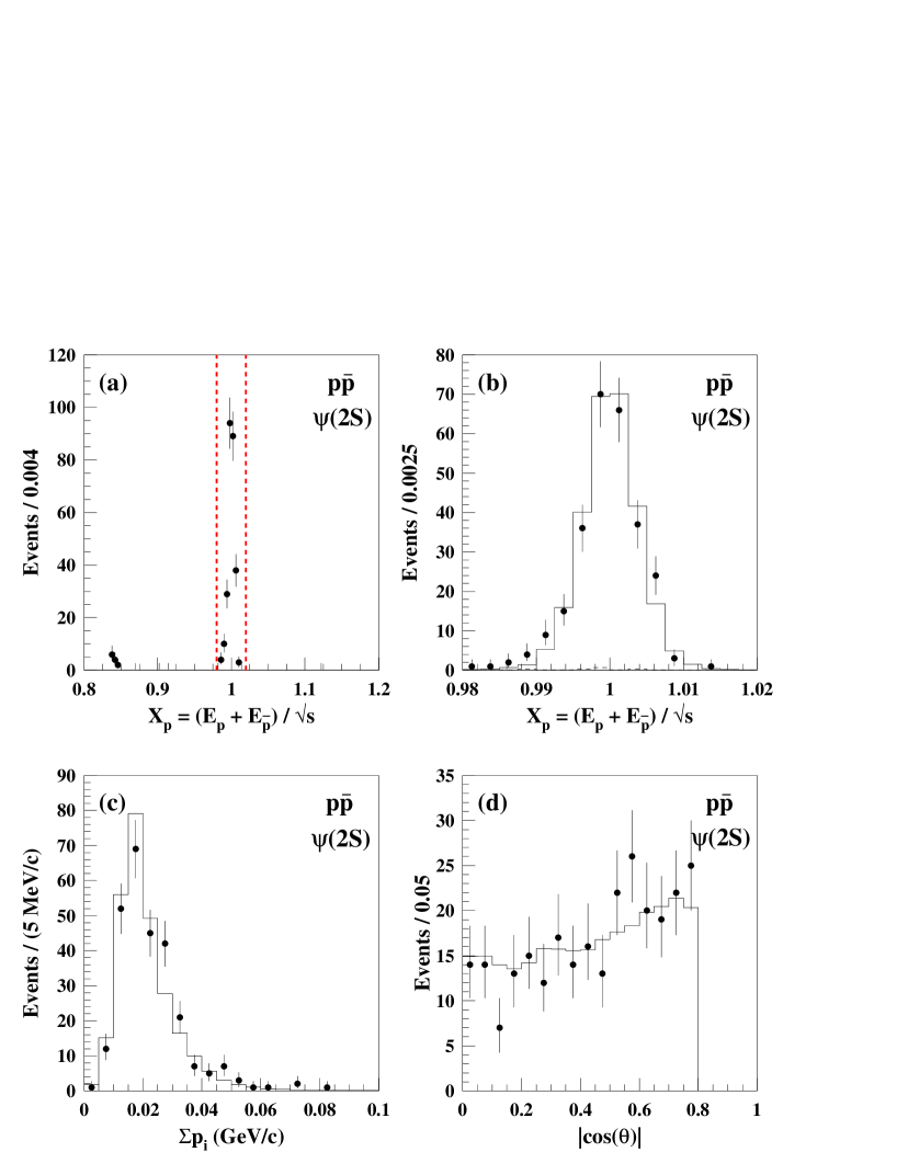
Figure 4.29: The $\psi(2S)$ data with the $p\overline{p}$ final state criteria applied. The points are data events. The solid histograms are $e^{+}e^{-}\rightarrow p\overline{p}$ signal MC, normalized to the number of observed events in the signal region. Figure (a): $X_{p}$ distribution. The $X_{p}$ signal region is enclosed by the dashed lines. Figure (b): $X_{p}$ signal region. The dashed histogram is the continuum data scaled according to Eqn. 4.26. Figure (c): Net momentum of the two tracks. Figure (d): $|$cos($\theta$)$|$ for the positive track.

The number of $e^{+}e^{-}\rightarrow p\overline{p}$ events in the $\psi(2S)$ data sample is

$$N^{\psi(2S)}_{cont}=A_{5}[(16.0^{+4.8}_{-3.7})-(1.94\pm 0.18)]=1.9\pm 0.6.$$

Note that the $l^{+}l^{-}$ contamination is negligible in both the continuum and $\psi(2S)$ data samples, as discussed at the end of Section 4.5.3. The number of $\psi(2S)\rightarrow p\overline{p}$ signal events is

$$N(\psi(2S)\rightarrow p\overline{p})=(269.0\pm 16.4)-(1.9\pm 0.6)=267.1\pm 16.4.$$

From Eqn. 4.23, the $\psi(2S)\rightarrow p\overline{p}$ branching ratio is

$${\cal{B}}(\psi(2S)\rightarrow p\overline{p})=\frac{267.1\pm 16.4}{(0.626)(1.52\times 10^{6})}=(2.81\pm 0.17(stat))\times 10^{-4}.$$

This value of ${\cal{B}}(\psi(2S)\rightarrow p\overline{p})$ is 2.4$\sigma$ larger than the PDG value of ${\cal{B}}(\psi(2S)\rightarrow p\overline{p})$ = $(2.07\pm 0.31)\times 10^{-4}$ [2] but is in good agreement with the E760 result ${\cal{B}}(\psi(2S)\rightarrow p\overline{p})$ = $(2.61^{+0.31}_{-0.21}\pm 0.17\pm 0.17)\times 10^{-4}$ [198]. Assuming $|G^{P}_{E}(s)|$ = $|G^{P}_{M}(s)|$ decreases the branching ratio by 0.04$\%$.

4.8.8 Determination of $\sigma(e^{+}e^{-}\rightarrow p\overline{p})$ and $|G^{P}_{M}(s)|$

Figure 4.30 shows the event distributions for several variables for the continuum data and signal MC after applying the $p\overline{p}$ event selection criteria under the two assumptions $|G^{P}_{E}(s)|$ = 0 and $|G^{P}_{E}(s)|$ = $|G^{P}_{M}(s)|$. There are 16 observed events in the $p\overline{p}$ signal region. The distributions of the data events are in agreement with both MC predictions, which differ very little.

Figure 4.30: Continuum data sample with the $p\overline{p}$ final state criteria applied. The points are data events. The solid histograms are the $e^{+}e^{-}\rightarrow p\overline{p}$ signal MC obtained with $|G^{P}_{E}(s)|$ = 0, and the dashed histograms are the $e^{+}e^{-}\rightarrow p\overline{p}$ signal MC obtained with $|G^{P}_{E}(s)|$ = $|G^{P}_{M}(s)|$ . The signal MC samples are normalized to the number of observed events in the signal region. Figure (a): $X_{p}$ distribution. The $X_{p}$ signal region is enclosed by the dashed lines. Figure (b): $X_{p}$ signal region. Figure (c): Net momentum of the two tracks. Figure (d): $|$cos($\theta$)$|$ for the positive track.

The values of all measured quantities for the 16 observed events are listed in Tables A.11-20 of Appendix A. The $E_{tkCC}/p$ values for the antiproton candidates are listed in Table A.20. The $E_{tkCC}/p$ $<$ 0.85 requirement is applied only to the protons, and not to the antiprotons because of their possible annihilation in the CC. Table A.20 shows that 5 of the 16 antiproton candidates have an $E_{tkCC}/p$ $>$ 0.85, consistent with the expectation of annihilation.

The number of $\psi(2S)\rightarrow p\overline{p}$ events in the continuum data sample is

$$N^{cont}_{\psi(2S)}=C^{\pi^{+}\pi^{-}J/\psi}[(269.0\pm 16.4)-(2.1^{+0.6}_{-0.5})]=1.92\pm 0.18.$$

Note that the $l^{+}l^{-}$ contamination is negligible in both the continuum and $\psi(2S)$ data samples, as discussed at the end of Section 4.5.3. The number of $e^{+}e^{-}\rightarrow p\overline{p}$ signal events is

$$N^{cont}(e^{+}e^{-}\rightarrow p\overline{p})=(16.0^{+4.8}_{-3.7})-(1.92\pm 0.18)=14.1^{+4.8}_{-3.7}.$$

Therefore, using Eqn. 4.28, the cross section for $e^{+}e^{-}\rightarrow p\overline{p}$ is

$$\sigma_{0}(e^{+}e^{-}\rightarrow p\overline{p})=\frac{14.1^{+4.8}_{-3.7}}{(0.626)(0.853)(20.7~{}\mathrm{pb^{-1}})}=1.27^{+0.43}_{-0.33}~{}\mathrm{pb},~{}~{}~{}~{}~{}~{}~{}~{}~{}~{}~{}~{}~{}(~{}|G^{P}_{E}(s)|=0~{})$$

and

$$\sigma_{0}(e^{+}e^{-}\rightarrow p\overline{p})=\frac{14.1^{+4.8}_{-3.7}}{(0.657)(0.860)(20.7~{}\mathrm{pb^{-1}})}=1.20^{+0.41}_{-0.31}~{}\mathrm{pb},~{}~{}~{}~{}(~{}|G^{P}_{E}(s)|=|G^{P}_{M}(s)|~{}).$$

Solving Eqn. 4.20 for $|G^{P}_{M}(s)|$ gives

$$|G^{P}_{M}(s)|=\sqrt{\frac{3s}{4\pi\alpha^{2}}\frac{\sigma_{0}(e^{+}e^{-}\rightarrow p\overline{p})}{\beta_{p}(1+\frac{2m^{2}_{p}}{s}\frac{|G^{P}_{E}(s)|^{2}}{|G^{P}_{M}(s)|^{2}})}}.$$ (4.36)

The magnetic form factor of the proton is therefore

$$|G^{P}_{M}(13.48~{}\mathrm{GeV}^{2})|=\sqrt{\frac{1.27^{+0.43}_{-0.33}~{}\mathrm{pb}}{5542~{}\mathrm{pb}}}=0.0152^{+0.0026}_{-0.0020},~{}~{}~{}~{}~{}~{}~{}~{}~{}~{}\mathrm{assuming}~{}(~{}|G^{P}_{E}(s)|=0~{}),$$

and

$$|G^{P}_{M}(13.48~{}\mathrm{GeV}^{2})|=\sqrt{\frac{1.20^{+0.41}_{-0.31}~{}\mathrm{pb}}{6266~{}\mathrm{pb}}}=0.0139^{+0.0024}_{-0.0018},~{}\mathrm{assuming}~{}(~{}|G^{P}_{E}(s)|=|G^{P}_{M}(s)|~{}).$$

where all errors are statistical only.

Due to the low statistics, a definitive measurement of the $|G^{P}_{E}(s)|/|G^{P}_{M}(s)|$ ratio is not possible from our data. A rough measurement can be done by calculating the ratio of the number of events with $|$cos$\theta|<0.5$ to the events with $0.5<|$cos$\theta|<0.8$ from the continuum data and comparing it to the ratio obtained from the $|G^{P}_{E}(s)|$ = 0 and $|G^{P}_{E}(s)|$ = $|G^{P}_{M}(s)|$ MC samples. The experimental ratio is found to be 0.78${}^{+0.49}_{-0.38}$. The MC results are 1.282$\pm$0.023 for $|G^{P}_{E}(s)|$ = 0, and 1.416$\pm$0.025 for $|G^{P}_{E}(s)|$ = $|G^{P}_{M}(s)|$. It is clear that our data does not have the statistical precision to distinguish between the two.

4.9 Systematic Uncertainties

Various sources of systematic uncertainty arise from possible biases in the event selection criteria, the treatment of the leptonic background, the treatment $\psi(2S)$ contamination in the continuum data sample, the statistical uncertainty in the detection efficiency, the bremstrahlung energy cutoff in the radiative correction, and the uncertainty in the luminosity.

The trigger uncertainty was studied in Ref. [184] for events with only two hard tracks and determined to be at most 0.62$\%$. A conservative estimate of the trigger uncertainty is taken to be 1$\%$.

Tracking uncertainties was studied in Ref. [192] and, again for the case of two hard tracks, in Ref. [184]. A tracking uncertainty of 0.7$\%$ was found for charged kaons, but a study of hard $\mu$ tracks in $\psi(2S)$ $\rightarrow$ $X$ $J/\psi$, $J/\psi$ $\rightarrow$ $\mu^{+}\mu^{-}$ decays determined an uncertainty of 1.0$\%$. The tracking uncertainty per track is taken to be 1$\%$.

The biases imposed by the signal region, net momentum, and $E_{tkCC}$ criteria are studied by varying the cuts, recalculating the efficiency, leptonic background, and radiative correction, and stating the difference in the cross section as a systematic uncertainty. Tables 4.11 and 4.12 list their effect on $\sigma_{0}(e^{+}e^{-}\rightarrow\pi^{+}\pi^{-})$ and $\sigma_{0}(e^{+}e^{-}\rightarrow K^{+}K^{-})$, respectively. For $\sigma_{0}(e^{+}e^{-}\rightarrow p\overline{p})$, Table 4.13 lists their effect on $e^{+}e^{-}\rightarrow p\overline{p}$ events with the assumption $|G^{P}_{E}(s)|$ = 0 and Table 4.14 lists their effect on $e^{+}e^{-}\rightarrow p\overline{p}$ events with the assumption $|G^{P}_{E}(s)|$ = $|G^{P}_{M}(s)|$. The final results are listed in Table 4.15.

Table 4.11: Systematic uncertainties in $\sigma_{0}(e^{+}e^{-}\rightarrow\pi^{+}\pi^{-})$ from signal region, net momentum, and $E_{tkCC}$ variation. The larger variation is taken as the systematic uncertainty.

$X_{\pi}$ Signal Region	$\sigma_{0}(e^{+}e^{-}\rightarrow\pi^{+}\pi^{-})$ (pb)	Change ($\%$)
$0.98<X_{\pi}<1.02$ (nominal)	9.045	—
$0.985<X_{\pi}<1.015$	9.416	$+4.1$
$0.975<X_{\pi}<1.025$	8.846	$-2.2$
Net momentum (MeV/$c$)
$\Sigma p_{i}<$ 100 (nominal)	9.045	—
$\Sigma p_{i}<$ 60	9.479	$+4.8$
$\Sigma p_{i}<$ 150	9.009	$-0.4$
$E_{tkCC}$ (MeV)
$E_{tkCC}<$ 420 (nominal)	9.045	—
$E_{tkCC}<$ 540	10.013	$+10.7$
$E_{tkCC}<$ 380	8.737	$-3.4$

Table 4.12: Systematic uncertainties in $\sigma_{0}(e^{+}e^{-}\rightarrow K^{+}K^{-})$ from signal region and net momentum variation. The larger variation is taken as the systematic uncertainty.

$X_{K}$ Signal Region	$\sigma_{0}(e^{+}e^{-}\rightarrow K^{+}K^{-})$ (pb)	Change ($\%$)
$0.98<X_{K}<1.02$ (nominal)	5.687	—
$0.985<X_{K}<1.015$	5.657	$-0.5$
$0.975<X_{K}<1.025$	5.666	$-0.4$
Net momentum (MeV/$c$)
$\Sigma p_{i}<$ 60 (nominal)	5.687	—
$\Sigma p_{i}<$ 50	5.770	$+1.5$
$\Sigma p_{i}<$ 80	5.541	$-2.6$

Table 4.13: Systematic uncertainties in $\sigma_{0}(e^{+}e^{-}\rightarrow p\overline{p})$ for $|G^{P}_{E}(s)|$ = 0 from signal region and net momentum variation. The larger variation is taken as the systematic uncertainty.

$X_{p}$ Signal Region	$\sigma_{0}(e^{+}e^{-}\rightarrow p\overline{p})$ (pb)	Change ($\%$)
$0.98<X_{p}<1.02$ (nominal)	1.274	—
$0.985<X_{p}<1.015$	1.321	$+3.7$
$0.975<X_{p}<1.025$	1.248	$-2.0$
Net momentum (MeV/$c$)
$\Sigma p_{i}<$ 100 (nominal)	1.274	—
$\Sigma p_{i}<$ 60	1.326	$+4.1$
$\Sigma p_{i}<$ 150	1.360	$+6.8$

Table 4.14: Systematic uncertainties in $\sigma_{0}(e^{+}e^{-}\rightarrow p\overline{p})$ for $|G^{P}_{E}(s)|$ = $|G^{P}_{M}(s)|$ from signal region and net momentum variation. The larger variation is taken as the systematic uncertainty.

$X_{p}$ Signal Region	$\sigma_{0}(e^{+}e^{-}\rightarrow p\overline{p})$ (pb)	Change ($\%$)
$0.98<X_{p}<1.02$ (nominal)	1.204	—
$0.985<X_{p}<1.015$	1.249	$+3.7$
$0.975<X_{p}<1.025$	1.179	$-2.0$
Net momentum (MeV/$c$)
$\Sigma p_{i}<$ 100 (nominal)	1.204	—
$\Sigma p_{i}<$ 60	1.252	$+4.0$
$\Sigma p_{i}<$ 150	1.287	$+6.9$

The uncertainty in the $dE/dx$+RICH PID criteria is determined by studying a substantial statistical sample of pion, kaon, and proton tracks at the desired momenta. The only source of such samples are from $D^{0}$ $\rightarrow$ $K^{-}\pi^{+}$ decays for charged pions and kaons and $\Lambda$ $\rightarrow$ $p\pi$ decays for protons with data taken at $\sqrt{s}$ = 10.58 GeV with the CLEO III detector (note that charge conjugation is implied for $D^{0}$ and $\Lambda$ and their decays). The PID uncertainty is studied by calculating the efficiencies for finding $D^{0}$s and $\Lambda$s using the method and resources described in Ref. [199]. Either the mean value, or the uncertainty, of the difference between the CLEO III data and MC efficiency for a particular particle type is taken as the systematic uncertainty per track. For pions with track momenta of $\sim$1.83 GeV/c, the difference is $-2.7\pm 1.9\%$; for kaons with track momenta of $\sim$1.77 GeV/c, the difference is $+0.2\pm 1.2\%$; and for protons with track momenta of $\sim$1.58 GeV/c, the difference is $-1.2\pm 1.6\%$. Therefore, the pion, kaon, and proton PID criteria is assigned a 2.7$\%$, 1.2$\%$, and 1.6$\%$ uncertainty per track, respectively.

The uncertainty in the pion identification efficiency from the $E_{tkCC}$ criteria is 2.3$\%$ per track and is described in Section 4.5.1.

Uncertainties from the $\psi(2S)$ contamination, leptonic background, and statistical uncertainty in efficiency determination due to finite MC sample sizes is determined by individually varying the mean values by $\pm 1\sigma$. The uncertainty in the bremstrahlung energy cutoff in the radiative correction is determined by varying the cutoff energy by a factor of two, i.e., changing $E_{\gamma,min}$ to 5 keV and 20 keV. The results are listed in Table 4.15.

The determination of the continuum data luminosity systematic uncertainty is documented in Ref. [181] and is determined to be 1$\%$.

The individual and total systematic uncertainties for $\sigma_{0}(e^{+}e^{-}\rightarrow h\overline{h})$ are summarized in Table 4.15. The total uncertainty is determined by a sum in quadrature of all individual contributions. The total systematic uncertainty on $\sigma_{0}(e^{+}e^{-}\rightarrow\pi^{+}\pi^{-})$ is 14.6$\%$, in $\sigma_{0}(e^{+}e^{-}\rightarrow K^{+}K^{-})$ it is 4.4$\%$, in $\sigma_{0}(e^{+}e^{-}\rightarrow p\overline{p})$ for $|G^{P}_{E}(s)|$ = 0 it is $8.8\%$ and for $|G^{P}_{E}(s)|$ = $|G^{P}_{M}(s)|$ it is $8.9\%$.

Table 4.15: Sources of systematic uncertainty for $\sigma_{0}(e^{+}e^{-}\rightarrow h\overline{h})$. The values are listed as percentages. The total uncertainty is determined by a sum in quadrature of all individual contributions.

Source	$\pi^{+}\pi^{-}$	$K^{+}K^{-}$	$p\overline{p}$	$p\overline{p}$
			$(\frac{|G^{P}_{E}(s)|}{|G^{P}_{M}(s)|}=0)$	$(\frac{|G^{P}_{E}(s)|}{|G^{P}_{M}(s)|}=1)$
Trigger	1.0	1.0	1.0	1.0
Tracking	2$\times$1.0	2$\times$1.0	2$\times$1.0	2$\times$1.0
$X_{h}$ Signal Region	4.1	0.5	3.7	3.7
Net Momentum	4.8	2.6	6.8	6.9
$E_{tkCC}$	10.7	—	—	—
$E_{tkCC}/p$	$>$0.1	$>$0.1	$>$0.1	$>$0.1
$dE/dx$+RICH PID	2$\times$2.7	2$\times$1.2	2$\times$1.6	2$\times$1.6
$\epsilon_{\pi}(E_{tkCC})$	2$\times$2.3	—	—	—
$\psi(2S)$ Contam	$>$0.1	0.1	0.9	1.0
Leptonic BG	$>$0.1	0.3	$>$0.1	$>$0.1
MC statistics	1.3	0.4	0.5	0.5
$x_{min}$	0.2	0.2	0.2	0.2
$\cal{L}$	1.0	1.0	1.0	1.0
Total ($\%$)	14.6	4.4	8.8	8.9

Chapter 5 Conclusions

Using the 20.7 pb^-1 of $e^{+}e^{-}$ data collected at $\sqrt{s}$ = 3.671 GeV, the electromagnetic form factors of the pion, kaon, and proton have been measured at a timelike momentum transfer of $|Q^{2}|=s$ = 13.48 GeV². The results are

$$|F_{\pi}(13.48~{}\mathrm{GeV}^{2})|=0.075\pm 0.008(stat)\pm 0.005(syst),$$

$$|F_{K}(13.48~{}\mathrm{GeV}^{2})|=0.063\pm 0.004(stat)\pm 0.001(syst),$$

and, assuming $|G^{P}_{E}(Q^{2})|$ = $|G^{P}_{M}(Q^{2})|$,

$$|G^{P}_{M}(13.48~{}\mathrm{GeV}^{2})|=0.0139^{+0.0024}_{-0.0018}(stat)\pm 0.0006(syst).$$

In order to facilitate comparison with PQCD predictions, equivalently

$$|Q^{2}||F_{\pi}(13.48~{}\mathrm{GeV}^{2})|=(1.01\pm 0.11(stat)\pm 0.07(syst))~{}\mathrm{GeV}^{2},$$ (5.1)

$$|Q^{2}||F_{K}(13.48~{}\mathrm{GeV}^{2})|=(0.85\pm 0.05(stat)\pm 0.02(syst))~{}\mathrm{GeV}^{2},$$ (5.2)

and

$$|Q^{4}||G^{P}_{M}(13.48~{}\mathrm{GeV}^{2})|/\mu_{p}=(0.91^{+0.16}_{-0.12}(stat)\pm 0.04(syst))~{}\mathrm{GeV}^{4}.$$ (5.3)

The results are displayed in Figures 5.1, 5.2, and 5.3 as $|Q^{2}||F_{\pi}|$, $|Q^{2}||F_{K}|$, and
$|Q^{4}||G_{M}^{p}|/\mu_{p}$, together with the existing world data for the same.

Figure 5.1: Experimental status of the pion form factors with timelike momentum transfer. The solid points are from $e^{+}e^{-}\rightarrow\pi^{+}\pi^{-}$ measurements with pions experimentally identified [28]-[33]. The open points are from $e^{+}e^{-}\rightarrow h^{+}h^{-}$ measurements with the pion fraction of the observed $h^{+}h^{-}$ determined according to a VDM prescription [34]. The value denoted with the triangle comes from interpreting the $J/\psi\rightarrow\pi^{+}\pi^{-}$ branching ratio as a pion form factor measurement as in Ref. [114]. The result from the present analysis is denoted by the open square. The arbitrarily normalized solid line shows the variation of $\alpha_{s}(|Q^{2}|)$ using its two-loop form with $n_{f}$ = 4 and $\Lambda$ = 0.322 GeV. The dashed and dash-dotted lines are the timelike PQCD predictions by Brodsky $\it{et~{}al.}$ [44] and Gousset and Pire [113], respectively. The dotted line is the timelike QCD Sum Rules (QCDSR) prediction by Bakulev $\it{et~{}al.}$ [115].

Figure 5.2: Experimental status of the kaon form factors with timelike momentum transfer. The solid points are from $e^{+}e^{-}\rightarrow K^{+}K^{-}$ measurements with kaons experimentally identified [28]-[30], [48]-[51]. The open points are from $e^{+}e^{-}\rightarrow h^{+}h^{-}$ measurements with the kaon fraction of the observed $h^{+}h^{-}$ determined according to a VDM prescription [19]. The value denoted with the triangle comes from interpreting the $J/\psi\rightarrow K^{+}K^{-}$ decay via a virtual photon as a kaon form factor measurement, as described in the text. The result from the present analysis is denoted by the open square. The vertical dotted line specifies the threshold for $K^{+}K^{-}$ production, i.e., $|Q^{2}|$ = $(2m_{K})^{2}$ = 0.975 GeV². The arbitrarily normalized solid line shows the variation of $\alpha_{s}(|Q^{2}|)$ using its two-loop form with $n_{f}$ = 4 and $\Lambda$ = 0.322 GeV.

Figure 5.3: Experimental status of the proton magnetic form factor with timelike momentum transfer assuming $|G^{P}_{E}(Q^{2})|$ = $|G^{P}_{M}(Q^{2})|$. The solid points are from $p\overline{p}$ final state measurements [54]-[62], while the stars are the E760/E835 measurements from $p\overline{p}\rightarrow e^{+}e^{-}$ events [63]-[65]. The result from the present analysis is denoted by the open square. The ellipse represents the variation of the central value with the different assumptions of $|G^{P}_{E}(Q^{2})|$ listed in Table 5.1. The vertical dotted line specifies the threshold for $p\overline{p}$ production, i.e., $|Q^{2}|$ = $(2m_{p})^{2}$ = 3.52 GeV². The arbitrarily normalized solid line shows the variation of $\alpha_{s}^{2}(|Q^{2}|)$ using its two-loop form with $n_{f}$ = 4 and $\Lambda$ = 0.322 GeV. The dashed line is the fit result of the variation of $\alpha_{s}^{2}(|Q^{2}|)$ for the spacelike momentum transfer data.

The precision result for $|Q^{2}||F_{\pi}(13.48~{}\mathrm{GeV}^{2})|$ is the first such directly measured result. Figure 5.3 shows that the PQCD predictions by Gousset and Pire [113] and Brodsky $\it{et~{}al.}$ [44] are factor two and three smaller than our result, respectively. The prediction by Bakulev $\it{et~{}al.}$ [115], based on the QCD Sum Rules, is also lower than our result. Our result also provides empirical validity for $|Q^{2}||F_{\pi}(9.6\;\mathrm{GeV}^{2})|=(0.94\pm 0.06)$ GeV² obtained by interpreting $\Gamma(J/\psi\to\pi^{+}\pi^{-})/\Gamma(J/\psi\to e^{+}e^{-})$ as a measure of the form factor [114]. Together, the two appear to support the PQCD prediction of $\alpha_{s}(|Q^{2}|)/|Q^{2}|$ variation of the form factor at large $Q^{2}$. Bebek $\it{et~{}al.}$ [42] have reported $Q^{2}F_{\pi}(9.77~{}\mathrm{GeV}^{2})$ = 0.69$\pm$0.19 GeV² for the spacelike form factor. Within errors this is consistent with being nearly factor two smaller than the timelike form factors for $Q^{2}>9$ GeV², as found for protons.

The measurement of the kaon form factor stands alone at present. While no explicit predictions exist for the kaon form factor in the timelike region, the $\alpha_{s}(|Q^{2}|)$ and $|Q^{2}|$ independent PQCD prediction [24] $|F_{K}(Q^{2})|/|F_{\pi}(Q^{2})|$ = $f_{K}^{2}/f_{\pi}^{2}$ = 1.49$\pm$0.03 is in disagreement with our result $|F_{K}(13.48\;\mathrm{GeV}^{2})|/|F_{\pi}(13.48~{}\mathrm{GeV}^{2})|$ = 0.84$\pm$0.11. Chernyak and Zhitnitsky [95] use the PQCD factorization scheme, but with two-humped distribution amplitudes obtained by the QCD Sum Rules. They obtain a factor 2/3 multiplying $f_{K}^{2}/f_{\pi}^{2}$ and predict $|F_{K}(Q^{2})|/|F_{\pi}(Q^{2})|$ = 0.99$\pm$0.02, which is consistent with our result within errors. However, the discrepancy between our experimental results and the PQCD based theoretical predictions has to be considered as unexplained.

Seth [200] has pointed out that because the $J/\psi\rightarrow K^{+}K^{-}$ decay can proceed through a virtual photon as well as three gluons, and the two decays have been shown to be orthogonal [201, 202], the measured ${\cal B}(J/\psi\rightarrow K^{+}K^{-})$ can be related to the kaon form factor after removing the contribution from the three gluon decay. The $J/\psi\rightarrow K^{+}K^{-}$ branching fraction can be written in terms of the amplitudes for the one photon $A_{\gamma}$ and three gluon $A_{ggg}$ decay as [202]

$${\cal B}(J/\psi\rightarrow K^{+}K^{-})=|A_{\gamma}+A_{ggg}|^{2}=|A_{\gamma}|^{2}+|A_{ggg}|^{2}={\cal B}_{~{}~{}\gamma}^{K^{+}K^{-}}+{\cal B}_{~{}ggg}^{K^{+}K^{-}},$$ (5.4)

where ${\cal B}_{~{}~{}\gamma}^{K^{+}K^{-}}$ and ${\cal B}_{~{}ggg}^{K^{+}K^{-}}$ are the branching fractions for the one photon and three gluon components of the $J/\psi\rightarrow K^{+}K^{-}$ decay. Using the assumption that the decay $J/\psi\rightarrow K^{0}_{S}K^{0}_{L}$ only occurs through the three gluon channel, its branching fraction can be used to determine ${\cal B}_{~{}ggg}^{K^{+}K^{-}}$. The one photon component is related to the kaon form factor by [203]

$${\cal B}_{~{}~{}\gamma}^{K^{+}K^{-}}=2{\cal B}(J/\psi\rightarrow e^{+}e^{-})\left(\frac{p_{K}}{M_{J/\psi}}\right)^{3}|F_{K}(M^{2}_{J/\psi})|^{2},$$ (5.5)

where $(p_{K}/M_{J/\psi})^{3}=0.106$ is the phase space factor, $p_{K}$ is the kaon momentum in the $J/\psi$ rest frame, and $M_{J/\psi}$ and ${\cal B}(J/\psi\rightarrow e^{+}e^{-})$ are the mass and the $e^{+}e^{-}$ branching fraction of $J/\psi$, respectively. Using the PDG values [2] of ${\cal B}(J/\psi\rightarrow K^{+}K^{-})=(2.37\pm 0.31)^{-4}$, ${\cal B}_{~{}ggg}^{K^{+}K^{-}}={\cal B}(J/\psi\rightarrow K^{0}_{S}K^{0}_{L})=(1.46\pm 0.26)^{-4}$, ${\cal B}(J/\psi\rightarrow e^{+}e^{-})=0.0593\pm 0.0010$, and $M_{J/\psi}=3096.916\pm 0.011$ MeV, the kaon form factor at $|Q^{2}|=M^{2}_{J/\psi}=9.6$ GeV² is

$$|Q^{2}||F_{K}(9.6~{}\mathrm{GeV}^{2})|=(0.81\pm 0.18)~{}\mathrm{GeV}^{2}.$$

This result is consistent with our result,

$$|Q^{2}||F_{K}(13.48~{}\mathrm{GeV}^{2})|=(0.85\pm 0.05(stat)\pm 0.02(syst))~{}\mathrm{GeV}^{2},$$

as shown in Figure 5.2. Using $|Q^{2}||F_{\pi}(9.6\;\mathrm{GeV}^{2})|=(0.94\pm 0.06)$ GeV² [114], the form factor ratio $|F_{K}(9.6~{}\mathrm{GeV}^{2})|/|F_{\pi}(9.6~{}\mathrm{GeV}^{2})|$ = 0.86$\pm$0.20 is also consistent with our experimental result, 0.84$\pm$0.11, at $|Q^{2}|=13.48$ GeV² and smaller than the theoretical predictions discussed above. Together, the two also appear to support the PQCD prediction of $\alpha_{s}(|Q^{2}|)/|Q^{2}|$ variation of the form factor at large $Q^{2}$.

The result for $|G^{P}_{M}(13.48~{}\mathrm{GeV}^{2})|$ is in excellent agreement with the results of the Fermilab E760/E835 experiments in which the reverse reaction $p\bar{p}\to e^{+}e^{-}$ was measured [63, 64, 65]. The result is also consistent with the magnetic form factor in the timelike region being twice as large as in the spacelike region.

The extraction of the experimental value of the proton magnetic form factor is dependent on the particular assumption of the electric form factor. The magnetic form factor has already been determined using two different assumptions: $|G^{P,tl}_{E}(Q^{2})|$ = 0 and $|G^{P,tl}_{E}(Q^{2})|$ = $|G^{P,tl}_{M}(Q^{2})|$, where the superscript $tl$ refers to timelike values. The recent measurements of the electric-to-magnetic form factor ratio in the spacelike region can be used to determine the same ratio in the timelike region by assuming that the Pauli-to-Dirac form factor ratio for the proton is the same in the spacelike and timelike regions. The electric-to-magnetic form factor ratio from the Rosenbluth measurements in the spacelike region is $G^{P,sl}_{E}(Q^{2})=G^{P,sl}_{M}(Q^{2})/\mu_{p}$, where the superscript $sl$ refers to spacelike values. This corresponds to $F^{P}_{2}(Q^{2})/F^{P}_{1}(Q^{2})=0.0855$, and leads to $|G^{P,tl}_{E}(Q^{2})|$ = 1.38 $|G^{P,tl}_{M}(Q^{2})|$. A linear extrapolation of the spacelike results from the polarization transfer measurements ($G^{P,sl}_{E}$(13.48 GeV²) = $-$0.8 $G^{P,sl}_{M}$(13.48 GeV²)$/\mu_{p}$) corresponds to $F^{P}_{2}(Q^{2})/F^{P}_{1}(Q^{2})=0.2027$, and leads $|G^{P,tl}_{E}(Q^{2})|$ = 1.75 $|G^{P,tl}_{M}(Q^{2})|$. The different assumptions of the electric form factor affect the differential and total cross sections and therefore the value of the magnetic form factor.

As mentioned earlier (Section 4.2), the differential cross section for $e^{+}e^{-}\rightarrow p\overline{p}$ is given by Eqn. 4.2 as

$$\frac{d\sigma_{0}}{d\Omega}\propto 1+B~{}\mathrm{cos}^{2}\theta,$$ (5.6)

where $B=(1-\eta)/(1+\eta)$ and

$$\eta=\frac{4m^{2}_{p}}{|Q^{2}|}\frac{|G^{P,tl}_{E}(Q^{2})|^{2}}{|G^{P,tl}_{M}(Q^{2})|^{2}}.$$ (5.7)

The corresponding total cross section is

$$\sigma_{0}=\frac{\pi\alpha^{2}}{3|Q^{2}|}~{}\beta_{p}(1+\eta)~{}[3+B]\times|G^{P,tl}_{M}(Q^{2})|^{2}~{}\equiv\sigma_{kin}~{}|G^{P,tl}_{M}(Q^{2})|^{2},$$ (5.8)

where $\sigma_{0}=N/[\epsilon(1+\delta){\cal L}]$, $N=14.1^{+4.8}_{-3.7}$, $(1+\delta)=0.856$, ${\cal L}$ = 20.7 pb^-1, and the efficiencies as listed in Table 5.1. Table 5.1 shows the results of the four different assumptions of $|G^{P,tl}_{E}(Q^{2})|/|G^{P,tl}_{M}(Q^{2})|$ on the present results for the $|G^{P,tl}_{M}(Q^{2})|$ measurement. It is interesting to note that with all these possible variations of $G^{P,sl}_{E}(Q^{2})/G^{P,sl}_{M}(Q^{2})$, $|Q^{4}||G^{P,tl}_{M}(Q^{2})|/\mu_{p}$ varies by only $\pm$0.1 GeV⁴, which is well within the errors of our measurement.

Table 5.1: Effect of different assumptions of $|G^{P,tl}_{E}(Q^{2})|/|G^{P,tl}_{M}(Q^{2})|$ on the extracted value of $|G^{P,tl}_{M}(Q^{2})|$. The variable $B$ is the coefficient of $\mathrm{cos}^{2}\theta$ in the differential cross section given by Eqn. 5.6. The $\sigma_{kin}$ and $|G^{P,tl}_{M}(Q^{2})|$ terms are determined from Eqn. 5.8. The errors are the statistical and systematic uncertainties summed in quadrature.

	$|G^{P,tl}_{E}(Q^{2})|/|G^{P,tl}_{M}(Q^{2})|$
	0	1	1.38	1.75
$B=(1-\eta)/(1+\eta)$	1	0.59	0.34	0.11
Efficiency: $\epsilon$	0.626	0.657	0.668	0.685
$\sigma_{0}$ (pb)	1.27${}^{+0.44}_{-0.35}$	1.21${}^{+0.42}_{-0.33}$	1.19${}^{+0.42}_{-0.33}$	1.16${}^{+0.41}_{-0.32}$
$\sigma_{kin}$ (pb)	5541	6265	6919	7757
$|G^{P,tl}_{M}(Q^{2})|$	0.0152${}^{+0.0027}_{-0.0021}$	0.0139${}^{+0.0025}_{-0.0019}$	0.0131${}^{+0.0023}_{-0.0018}$	0.0122${}^{+0.0022}_{-0.0017}$
$|Q^{4}||G^{P,tl}_{M}(Q^{2})|/\mu_{p}$	0.99${}^{+0.18}_{-0.14}$	0.91${}^{+0.16}_{-0.13}$	0.85${}^{+0.15}_{-0.12}$	0.79${}^{+0.14}_{-0.11}$
(GeV4)

Appendix A Event Lists for $e^{+}e^{-}\rightarrow\pi^{+}\pi^{-}$ and $e^{+}e^{-}\rightarrow p\overline{p}$ at $\sqrt{s}$ = 3.671 GeV

Tables A.1-10 list the properties of all 26 events included in the final event selection for the channel $e^{+}e^{-}\rightarrow\pi^{+}\pi^{-}$ as described in Chapter 4. Tables A.11-20 list the properties of all 16 events included in the final event selection for the channel $e^{+}e^{-}\rightarrow p\overline{p}$ as described in Chapter 4.

Table A.1: Properties of the events for the $e^{+}e^{-}\rightarrow\pi^{+}\pi^{-}$ final selection (Part 1). The variable $X_{\pi}$ is defined as $X_{\pi}\equiv(E(+)+E(-))/\sqrt{s}$, where $E(\pm)$ is $E(\pm)=\sqrt{|p(\pm)|^{2}+m^{2}_{\pi}}$. The variable $\Sigma p_{i}$ is the net momentum of the two tracks. Acolin is the acolinearity between the two tracks. The variables $p(+)$ and $p(-)$ are the momenta of the positive and negative tracks, respectively.

Run	Event	$X_{\pi}$	$\Sigma p_{i}$	Acolin	$p(+)$	$p(-)$
			(GeV/c)	(deg.)	(GeV/c)	(GeV/c)
203165	39815	0.999	0.039	0.407	1.810	1.848
203182	45425	0.992	0.023	0.391	1.806	1.826
203203	10540	0.996	0.025	0.427	1.832	1.811
203218	27556	1.002	0.020	0.558	1.830	1.839
203232	12545	1.003	0.036	0.306	1.852	1.818
203247	101424	1.008	0.017	0.531	1.845	1.845
203280	41768	1.007	0.013	0.383	1.845	1.841
203328	7923	0.991	0.022	0.583	1.819	1.808
203363	52988	1.008	0.035	0.508	1.860	1.829
203949	64635	1.003	0.013	0.159	1.841	1.830
203972	42766	1.003	0.016	0.484	1.837	1.834
204001	56773	1.012	0.019	0.161	1.861	1.843
204002	21854	0.998	0.019	0.585	1.827	1.826
204003	87811	0.998	0.012	0.284	1.830	1.822
204014	27853	1.000	0.005	0.155	1.831	1.831
204020	11274	0.999	0.016	0.492	1.826	1.829
204064	45495	1.006	0.020	0.419	1.848	1.833
204083	53808	0.999	0.031	0.166	1.844	1.813
204117	56203	0.998	0.009	0.287	1.828	1.826
204134	39364	0.997	0.023	0.501	1.817	1.833
204160	8433	0.993	0.022	0.479	1.810	1.825
204195	1949	0.996	0.031	0.578	1.811	1.836
204197	39119	1.007	0.027	0.673	1.851	1.835
204213	2886	1.005	0.021	0.291	1.848	1.830
204297	32047	1.002	0.021	0.626	1.837	1.831
204327	82333	1.001	0.020	0.532	1.827	1.837
Requirement		0.98$-$1.02	$<$ 0.100	—	—

Table A.2: Properties of the events for the $e^{+}e^{-}\rightarrow\pi^{+}\pi^{-}$ final selection (Part 2). The variables cos$\theta$, $\phi_{0}$, and $\chi^{2}/dof$ are the cosine of the angle between the charged track and the positron beam, the angle of the charged track in the plane perpendicular to the positron beam, and the reduced $\chi^{2}$ of the helix fit of the charged track, respectively. The $+$ and $-$ specify the charge of the track.

Run	Event	cos$\theta(+)$	cos$\theta(-)$	$\phi_{0}(+)$	$\phi_{0}(-)$	$\chi^{2}/dof(+)$	$\chi^{2}/dof(-)$
				(deg.)	(deg.)
203165	39815	-0.238	0.241	285.7	106.1	0.818	0.734
203182	45425	0.499	-0.494	37.4	217.1	0.861	0.880
203203	10540	0.063	-0.059	127.0	306.7	0.956	0.498
203218	27556	-0.250	0.258	226.0	46.3	0.831	1.208
203232	12545	0.585	-0.589	187.8	8.0	1.506	1.014
203247	101424	0.445	-0.436	10.6	190.5	1.032	0.775
203280	41768	0.595	-0.593	300.3	120.8	1.126	1.105
203328	7923	-0.315	0.324	169.4	349.1	0.887	1.334
203363	52988	0.378	-0.384	25.9	205.5	0.830	0.628
203949	64635	0.121	-0.120	200.4	20.7	0.783	1.098
203972	42766	-0.533	0.534	92.3	271.7	0.839	0.986
204001	56773	0.247	-0.245	357.5	177.4	1.352	1.395
204002	21854	0.346	-0.352	248.3	68.8	1.377	0.961
204003	87811	0.658	-0.655	174.8	354.7	1.046	0.941
204014	27853	0.152	-0.154	359.7	179.8	0.637	1.081
204020	11274	0.682	-0.677	57.6	237.1	0.689	0.953
204064	45495	0.584	-0.579	340.2	160.4	0.739	0.947
204083	53808	-0.486	0.486	208.9	29.1	0.791	1.185
204117	56203	-0.203	0.201	53.1	232.8	0.631	0.996
204134	39364	0.487	-0.488	332.3	152.9	1.273	1.542
204160	8433	0.266	-0.269	285.2	105.7	0.836	0.551
204195	1949	-0.345	0.343	275.3	95.9	0.971	0.832
204197	39119	0.397	-0.404	128.3	307.7	1.862	1.157
204213	2886	-0.469	0.473	191.0	11.1	1.333	0.694
204297	32047	0.119	-0.112	70.4	249.9	1.327	0.540
204327	82333	-0.735	0.729	350.4	170.5	1.072	0.858
Requirement		$|$cos$\theta(\pm)|$ $<$ 0.75		—		$\chi^{2}/dof(\pm)$ $<$ 10

Table A.3: Properties of the events for the $e^{+}e^{-}\rightarrow\pi^{+}\pi^{-}$ final selection (Part 3). The variables $d_{b}$ and $z_{b}$ are the distances between the origin of the helix fit and the position of the $e^{+}e^{-}$ annihilation in the plane perpendicular to and along the axis defined by the positron beam, respectively. DRHF is defined as the ratio of the number of Drift Chamber wire “hits” observed to the number of “hits” expected from the helix fit. The $+$ and $-$ specify the charge of the track.

Run	Event	$d_{b}(+)$	$d_{b}(-)$	$z_{b}(+)$	$z_{b}(-)$	DRHF(+)	DRHF(-)
		(mm)	(mm)	(cm)	(cm)
203165	39815	0.224	-0.105	0.330	0.205	0.907	0.907
203182	45425	-0.118	0.075	0.192	0.340	0.963	0.944
203203	10540	0.357	-0.132	-1.373	-1.344	0.963	0.963
203218	27556	-0.092	0.409	0.414	0.524	0.852	0.963
203232	12545	-0.090	-0.019	-1.335	-1.329	0.944	0.944
203247	101424	-0.083	0.013	-1.132	-0.917	0.944	0.981
203280	41768	0.101	0.048	-0.628	-0.618	0.944	0.963
203328	7923	0.012	-0.008	-0.314	0.206	0.870	0.926
203363	52988	-0.407	0.154	0.893	0.547	0.926	0.926
203949	64635	0.012	0.025	-0.880	-0.642	0.963	0.944
203972	42766	0.252	0.019	0.626	0.540	1.000	0.907
204001	56773	-0.291	-0.065	-0.628	-0.906	0.833	0.926
204002	21854	0.005	-0.302	-1.629	-1.691	0.963	0.926
204003	87811	-0.181	0.115	-0.390	-0.306	0.963	0.944
204014	27853	-0.048	-0.038	-1.045	-1.253	0.944	0.926
204020	11274	0.315	-0.496	1.179	1.293	0.963	0.963
204064	45495	-0.184	0.071	0.379	0.459	0.963	0.926
204083	53808	0.052	-0.127	0.797	0.559	0.907	0.944
204117	56203	-0.087	-0.008	0.320	0.388	0.889	0.963
204134	39364	0.176	-0.046	0.755	0.389	0.963	0.907
204160	8433	0.217	-0.268	-0.295	-0.157	0.944	0.926
204195	1949	-0.078	0.016	1.503	1.401	0.926	0.963
204197	39119	0.066	0.108	-0.148	-0.333	0.926	0.870
204213	2886	0.202	-0.035	-0.194	0.257	0.944	0.981
204297	32047	0.243	-0.186	1.100	1.024	0.926	0.907
204327	82333	-0.074	0.067	1.170	0.895	0.907	0.944
Requirement		$|d_{b}(\pm)|$ $<$ 5		$|z_{b}(\pm)|$ $<$ 5		0.5$-$1.2

Table A.4: Properties of the events for the $e^{+}e^{-}\rightarrow\pi^{+}\pi^{-}$ final selection (Part 4). The variables $S(i)$ [$i=e,\mu,\pi,K,p$] are the pulls based on the ionization energy loss ($dE/dx$) of the charged track in the Drift Chamber and are defined as $S(i)\equiv((dE/dx)_{\mathrm{meas}}-(dE/dx)_{\mathrm{expected,}i})/\sigma$. The measured $dE/dx$ of the charged track is $(dE/dx)_{\mathrm{meas}}$, the expected $dE/dx$ for particle hypothesis $i$ is $(dE/dx)_{\mathrm{expected,}i}$, and the uncertainty in the $dE/dx$ measurement is $\sigma$. The values below are for positive tracks only, the values for the negative tracks are given in Table A.5.

Run	Event	$S(e^{+})$	$S(\mu^{+})$	$S(\pi^{+})$	$S(K^{+})$	$S(p)$
203165	39815	-3.4158	-0.5323	-0.0014	1.4992	-0.0489
203182	45425	-4.8347	-1.9824	-1.4359	0.1406	-1.5020
203203	10540	-2.6720	0.2610	0.7919	2.2988	0.8366
203218	27556	-3.5736	-0.8540	-0.3457	1.1227	-0.3138
203232	12545	-3.5419	-0.5487	0.0076	1.6331	0.1378
203247	101424	-3.4473	-0.4866	0.0620	1.6538	0.1586
203280	41768	-3.7438	-0.7175	-0.1535	1.4903	-0.0502
203328	7923	-2.6994	0.1601	0.6775	2.1333	0.6690
203363	52988	-3.7028	-0.8622	-0.3285	1.2495	-0.1732
203949	64635	-4.8308	-1.9759	-1.4164	0.2250	-1.2822
203972	42766	-3.6171	-0.4889	0.0993	1.7808	0.2210
204001	56773	-2.1967	0.6125	1.1320	2.6073	1.3276
204002	21854	-3.2839	-0.3697	0.1738	1.7161	0.2373
204003	87811	-4.5225	-1.4148	-0.8195	0.8990	-0.7298
204014	27853	-2.6898	0.3253	0.8792	2.4377	0.9667
204020	11274	-3.8742	-0.7395	-0.1498	1.5327	-0.0774
204064	45495	-4.0482	-1.0278	-0.4488	1.2306	-0.2776
204083	53808	-2.7069	0.4102	0.9854	2.6120	1.1295
204117	56203	-2.7890	0.1844	0.7319	2.2740	0.8088
204134	39364	-2.6972	0.3675	0.9260	2.4852	0.9547
204160	8433	-3.6618	-0.7608	-0.2183	1.3183	-0.2196
204195	1949	-2.6643	0.3413	0.8878	2.4098	0.8935
204197	39119	-3.8755	-1.0414	-0.4966	1.0867	-0.3290
204213	2886	-4.4551	-1.4863	-0.9107	0.7699	-0.7440
204297	32047	-3.3744	-0.6618	-0.1488	1.3229	-0.0479
204327	82333	-2.7469	0.6104	1.2223	2.9337	1.2984

Table A.5: Properties of the events for the $e^{+}e^{-}\rightarrow\pi^{+}\pi^{-}$ final selection (Part 5). The variables $S(i)$ [$i=e,\mu,\pi,K,p$] are the pulls based on the ionization energy loss ($dE/dx$) of the charged track in the Drift Chamber and are defined as $S(i)\equiv((dE/dx)_{\mathrm{meas}}-(dE/dx)_{\mathrm{expected,}i})/\sigma$. The measured $dE/dx$ of the charged track is $(dE/dx)_{\mathrm{meas}}$, the expected $dE/dx$ for particle hypothesis $i$ is $(dE/dx)_{\mathrm{expected,}i}$, and the uncertainty in the $dE/dx$ measurement is $\sigma$. The values below are for negative tracks only, the values for the positive tracks are given in Table A.4.

Run	Event	$S(e^{-})$	$S(\mu^{-})$	$S(\pi^{-})$	$S(K^{-})$	$S(\overline{p})$
203165	39815	-3.6418	-0.8653	-0.3446	1.1810	-0.2407
203182	45425	-3.6141	-0.7130	-0.1742	1.3722	-0.1571
203203	10540	-4.4347	-1.5859	-1.0454	0.5104	-1.0899
203218	27556	-2.3698	0.5825	1.1130	2.6179	1.1840
203232	12545	-4.4078	-1.4868	-0.9339	0.6622	-0.9521
203247	101424	-3.3184	-0.2232	0.3461	1.9919	0.4501
203280	41768	-2.5923	0.6279	1.2069	2.8513	1.2911
203328	7923	-4.4856	-1.7139	-1.1859	0.3337	-1.2445
203363	52988	-2.9475	0.0653	0.6133	2.1694	0.6445
203949	64635	-2.0894	0.9977	1.5549	3.1043	1.6347
203972	42766	-2.8245	0.3217	0.9009	2.5340	1.0073
204001	56773	-3.4900	-0.6101	-0.0647	1.5029	0.0720
204002	21854	-3.5622	-0.5561	0.0071	1.6099	0.0742
204003	87811	-4.6514	-1.5548	-0.9618	0.7469	-0.9070
204014	27853	-4.4539	-1.6971	-1.1624	0.3934	-1.0748
204020	11274	-2.7461	0.6925	1.3191	3.0726	1.4103
204064	45495	-4.6621	-1.6189	-1.0318	0.6718	-0.9284
204083	53808	-4.5409	-1.5315	-0.9573	0.6904	-0.9424
204117	56203	-3.7167	-0.8560	-0.3151	1.2328	-0.2468
204134	39364	-3.1438	-0.1954	0.3541	1.9148	0.4497
204160	8433	-2.5479	0.5153	1.0738	2.6363	1.1388
204195	1949	-3.3511	-0.2538	0.3250	1.9726	0.4387
204197	39119	-2.3580	0.6411	1.1886	2.7242	1.2912
204213	2886	-5.0126	-2.0889	-1.5181	0.1484	-1.4308
204297	32047	-3.6854	-0.7180	-0.1581	1.4437	-0.0687
204327	82333	-4.0414	-0.8221	-0.2124	1.5379	-0.0889

Table A.6: Properties of the events for the $e^{+}e^{-}\rightarrow\pi^{+}\pi^{-}$ final selection (Part 6). This table deals with separating pions from electrons based on $dE/dx$ and RICH information. Columns 1 and 3 are $\Delta S^{2}(\pi$$-$$e)=S^{2}(\pi)-S^{2}(e)$ for positive and negative tracks, respectively. Columns 2 and 4 are $\Delta\chi^{2}_{RICH}(\pi$$-$$e)=-2$ log$L(\pi)+2$ log$L(e)$ for positive and negative tracks, respectively. Column 1+2 (3+4) is the sum of columns 1 and 2 (3 and 4). A track is more likely to be a pion than an electron if the value is $<$0.

Run	Event	1	2	1+2	3	4	3+4
203165	39815	-11.668	0.311	-11.356	-13.144	0.256	-12.887
203182	45425	-21.313	-0.040	-21.353	-13.031	0.345	-12.686
203203	10540	-6.512	0.577	-5.935	-18.573	-1.626	-20.199
203218	27556	-12.651	0.666	-11.985	-4.377	-0.242	-4.620
203232	12545	-12.545	0.899	-11.646	-18.556	-2.235	-20.792
203247	101424	-11.880	0.690	-11.190	-10.892	-1.909	-12.801
203280	41768	-13.992	-2.672	-16.665	-5.264	0.099	-5.164
203328	7923	-6.8277	-2.911	-9.739	-18.714	-0.372	-19.086
203363	52988	-13.603	0.208	-13.395	-8.312	-1.065	-9.377
203949	64635	-21.330	4.142	-17.189	-1.948	1.341	-0.607
203972	42766	-13.074	-0.245	-13.319	-7.166	-0.501	-7.667
204001	56773	-3.544	-0.442	-3.986	-12.176	-1.522	-13.699
204002	21854	-10.754	0.334	-10.420	-12.689	-1.952	-14.641
204003	87811	-19.781	-0.577	-20.358	-20.710	1.470	-19.241
204014	27853	-6.462	-2.439	-8.901	-18.486	6.159	-12.327
204020	11274	-14.987	0.450	-14.537	-5.801	0.216	-5.585
204064	45495	-16.187	2.926	-13.261	-20.671	0.084	-20.587
204083	53808	-6.356	-1.062	-7.418	-19.703	0.329	-19.374
204117	56203	-7.243	4.108	-3.135	-13.715	-2.932	-16.647
204134	39364	-6.4176	1.879	-4.538	-9.758	-0.296	-10.054
204160	8433	-13.361	-0.723	-14.084	-5.339	-1.246	-6.585
204195	1949	-6.310	0.027	-6.284	-11.124	1.420	-9.704
204197	39119	-14.773	-0.135	-14.907	-4.147	0.744	-3.403
204213	2886	-19.018	-0.740	-19.758	-22.822	-0.885	-23.707
204297	32047	-11.364	0.209	-11.156	-13.557	-1.601	-15.158
204327	82333	-6.0512	-0.534	-6.585	-16.288	-1.120	-17.407
Requirement		—	—	$<$ 0	—	—	$<$ 0

Table A.7: Properties of the events for the $e^{+}e^{-}\rightarrow\pi^{+}\pi^{-}$ final selection (Part 7). This table deals with separating pions from muons based on $dE/dx$ and RICH information. Columns 1 and 3 are $\Delta S^{2}(\pi$$-$$\mu)=S^{2}(\pi)-S^{2}(\mu)$ for positive and negative tracks, respectively. Columns 2 and 4 are $\Delta\chi^{2}_{RICH}(\pi$$-$$\mu)=-2$ log$L(\pi)+2$ log$L(\mu)$ for positive and negative tracks, respectively. Column 1+2 (3+4) is the sum of columns 1 and 2 (3 and 4). A track is more likely to be a pion than an muon if the value is $<$0.

Run	Event	1	2	1+2	3	4	3+4
203165	39815	-0.283	0.201	-0.082	-0.630	0.120	-0.510
203182	45425	-1.868	0.038	-1.831	-0.478	0.203	-0.275
203203	10540	0.559	0.316	0.875	-1.422	-0.588	-2.010
203218	27556	-0.610	0.373	-0.237	0.900	-0.023	0.876
203232	12545	-0.301	0.448	0.148	-1.338	-0.868	-2.207
203247	101424	-0.233	0.370	0.137	0.070	-0.736	-0.666
203280	41768	-0.491	-1.032	-1.523	1.062	0.110	1.173
203328	7923	0.433	-1.136	-0.703	-1.531	-0.072	-1.603
203363	52988	-0.635	0.152	-0.484	0.372	-0.416	-0.045
203949	64635	-1.898	3.450	1.552	1.422	0.681	2.103
203972	42766	-0.229	-0.038	-0.267	0.708	-0.156	0.553
204001	56773	0.906	-0.097	0.810	-0.368	-0.498	-0.866
204002	21854	-0.107	0.277	0.170	-0.309	-0.703	-1.012
204003	87811	-1.330	-0.170	-1.500	-1.492	0.678	-0.815
204014	27853	0.667	-1.015	-0.348	-1.529	4.920	3.391
204020	11274	-0.524	0.234	-0.291	1.261	0.120	1.380
204064	45495	-0.855	-0.400	-1.255	-1.556	0.086	-1.471
204083	53808	0.803	-0.357	0.446	-1.429	0.216	-1.213
204117	56203	0.502	0.080	0.581	-0.633	-1.099	-1.733
204134	39364	0.722	0.878	1.601	0.087	-0.041	0.047
204160	8433	-0.531	-0.239	-0.770	0.888	-0.405	0.483
204195	1949	0.672	0.124	0.796	0.041	0.680	0.721
204197	39119	-0.838	-0.009	-0.846	1.002	0.346	1.348
204213	2886	-1.380	-0.209	-1.589	-2.059	-0.310	-2.369
204297	32047	-0.416	0.180	-0.236	-0.490	-0.620	-1.110
204327	82333	1.121	-0.169	0.952	-0.631	-0.447	-1.077

Table A.8: Properties of the events for the $e^{+}e^{-}\rightarrow\pi^{+}\pi^{-}$ final selection (Part 8). This table deals with separating pions from kaons based on $dE/dx$ and RICH information. Columns 1 and 3 are $\Delta S^{2}(\pi$$-$$K)=S^{2}(\pi)-S^{2}(K)$ for positive and negative tracks, respectively. Columns 2 and 4 are $\Delta\chi^{2}_{RICH}(\pi$$-$$K)=-2$ log$L(\pi)+2$ log$L(K)$ for positive and negative tracks, respectively. Column 1+2 (3+4) is the sum of columns 1 and 2 (3 and 4). A track is more likely to be a pion than an kaon if the value is $<$0.

Run	Event	1	2	1+2	3	4	3+4
203165	39815	-2.248	-28.836	-31.083	-1.276	-7.619	-8.895
203182	45425	2.042	-23.463	-21.421	-1.853	-29.295	-31.147
203203	10540	-4.657	-38.716	-43.373	0.832	-15.533	-14.700
203218	27556	-1.141	-45.013	-46.154	-5.615	-24.845	-30.460
203232	12545	-2.667	-38.662	-41.329	0.434	-11.827	-11.393
203247	101424	-2.731	-31.920	-34.651	-3.848	-17.838	-21.686
203280	41768	-2.197	-22.150	-24.347	-6.674	-28.714	-35.388
203328	7923	-4.092	-16.930	-21.021	1.295	-23.840	-22.545
203363	52988	-1.453	-24.021	-25.475	-4.330	-7.901	-12.231
203949	64635	1.956	-61.203	-59.247	-7.219	-50.836	-58.054
203972	42766	-3.162	-28.373	-31.535	-5.609	-16.671	-22.280
204001	56773	-5.516	-28.234	-33.751	-2.254	-57.159	-59.413
204002	21854	-2.915	-42.901	-45.816	-2.592	-33.268	-35.860
204003	87811	-0.137	-25.477	-25.614	0.367	-33.886	-33.519
204014	27853	-5.169	-0.595	-5.765	1.196	-74.474	-73.278
204020	11274	-2.327	-19.427	-21.754	-7.701	-16.342	-24.043
204064	45495	-1.312	-29.268	-30.581	0.613	-20.971	-20.358
204083	53808	-5.852	-30.594	-36.445	0.440	-35.001	-34.562
204117	56203	-4.635	-38.807	-43.443	-1.421	-28.982	-30.402
204134	39364	-5.319	-44.112	-49.431	-3.541	-35.119	-38.660
204160	8433	-1.690	-24.125	-25.815	-5.797	-36.961	-42.758
204195	1949	-5.019	-48.936	-53.955	-3.786	-43.839	-47.624
204197	39119	-0.934	-18.757	-19.691	-6.009	-21.239	-27.247
204213	2886	0.237	-35.883	-35.646	2.283	-18.696	-16.414
204297	32047	-1.728	-38.732	-40.460	-2.059	-9.927	-11.986
204327	82333	-7.113	-22.856	-29.969	-2.320	-3.089	-5.409
Requirement		—	—	$<$ 0	—	—	$<$ 0

Table A.9: Properties of the events for the $e^{+}e^{-}\rightarrow\pi^{+}\pi^{-}$ final selection (Part 9). This table deals with separating pions from protons based on $dE/dx$ and RICH information. Columns 1 and 3 are $\Delta S^{2}(\pi$$-$$p)=S^{2}(\pi)-S^{2}(p)$ for positive and negative tracks, respectively. Columns 2 and 4 are $\Delta\chi^{2}_{RICH}(\pi$$-$$p)=-2$ log$L(\pi)+2$ log$L(p)$ for positive and negative tracks, respectively. Column 1+2 (3+4) is the sum of columns 1 and 2 (3 and 4). A track is more likely to be a pion than an proton if the value is $<$0.

Run	Event	1	2	1+2	3	4	3+4
203165	39815	-0.002	-70.294	-70.297	0.061	-21.822	-21.761
203182	45425	-0.194	-102.678	-102.872	0.006	-100.294	-100.288
203203	10540	-0.073	-115.476	-115.548	-0.095	-146.877	-146.972
203218	27556	0.021	-110.937	-110.916	-0.163	-82.639	-82.803
203232	12545	-0.019	-149.792	-149.811	-0.034	-128.522	-128.556
203247	101424	-0.021	-135.227	-135.249	-0.083	-129.667	-129.750
203280	41768	0.021	-195.545	-195.524	-0.210	-115.735	-115.945
203328	7923	0.012	-127.004	-126.993	-0.142	-80.387	-80.529
203363	52988	0.078	-85.402	-85.324	-0.039	-55.816	-55.856
203949	64635	0.362	-148.569	-148.207	-0.254	-129.155	-129.410
203972	42766	-0.039	-123.886	-123.925	-0.203	-91.949	-92.152
204001	56773	-0.481	-143.892	-144.373	-0.001	-141.017	-141.018
204002	21854	-0.026	-111.513	-111.539	-0.005	-117.623	-117.629
204003	87811	0.139	-110.106	-109.967	0.102	-116.477	-116.375
204014	27853	-0.161	-91.503	-91.665	0.196	-175.258	-175.062
204020	11274	0.016	-79.879	-79.863	-0.249	-64.357	-64.605
204064	45495	0.124	-154.176	-154.052	0.203	-85.709	-85.506
204083	53808	-0.305	-160.211	-160.516	0.028	-139.807	-139.779
204117	56203	-0.118	-110.080	-110.199	0.038	-139.011	-138.973
204134	39364	-0.054	-155.698	-155.752	-0.077	-165.091	-165.168
204160	8433	-0.001	-106.285	-106.286	-0.144	-172.356	-172.500
204195	1949	-0.010	-151.338	-151.348	-0.087	-103.506	-103.593
204197	39119	0.138	-88.223	-88.084	-0.254	-75.811	-76.065
204213	2886	0.276	-179.510	-179.234	0.257	-106.701	-106.444
204297	32047	0.020	-145.397	-145.377	0.020	-59.201	-59.180
204327	82333	-0.192	-135.996	-136.188	0.037	-58.977	-58.940

Table A.10: Properties of the events for the $e^{+}e^{-}\rightarrow\pi^{+}\pi^{-}$ final selection (Part 10). Columns 1 and 4 are $E_{tkCC}/p$ for positive and negative tracks, respectively. Columns 2 and 5 are $E_{tkCC}$ for positive and negative tracks, respectively. Columns 3 and 6 are the distances transversed in the Muon Chamber (in terms of nuclear interaction lengths) by positive and negative tracks, respectively.

Run	Event	1	2	3	4	5	6
			(GeV)			(GeV)
203165	39815	0.632	1.144	0.00	0.378	0.698	0.00
203182	45425	0.496	0.896	0.00	0.512	0.935	0.00
203203	10540	0.632	1.158	0.00	0.722	1.308	0.00
203218	27556	0.382	0.698	0.00	0.464	0.853	0.00
203232	12545	0.445	0.824	0.00	0.392	0.713	0.00
203247	101424	0.485	0.895	0.00	0.596	1.100	0.00
203280	41768	0.396	0.731	0.00	0.795	1.463	0.00
203328	7923	0.500	0.910	0.00	0.529	0.955	0.00
203363	52988	0.445	0.827	0.00	0.404	0.739	0.00
203949	64635	0.446	0.822	0.00	0.505	0.923	0.00
203972	42766	0.464	0.853	0.00	0.317	0.581	0.00
204001	56773	0.591	1.101	0.00	0.273	0.502	0.00
204002	21854	0.406	0.742	0.00	0.389	0.710	0.00
204003	87811	0.492	0.901	0.00	0.402	0.732	0.00
204014	27853	0.617	1.130	0.00	0.319	0.584	0.00
204020	11274	0.553	1.010	0.00	0.415	0.760	0.05
204064	45495	0.253	0.468	3.95	0.385	0.706	0.00
204083	53808	0.695	1.282	0.00	0.357	0.648	0.00
204117	56203	0.572	1.045	0.00	0.495	0.904	0.00
204134	39364	0.516	0.938	0.00	0.466	0.855	0.00
204160	8433	0.537	0.972	0.00	0.337	0.615	0.00
204195	1949	0.553	1.001	0.00	0.498	0.915	0.00
204197	39119	0.493	0.913	0.00	0.571	1.047	0.00
204213	2886	0.471	0.870	0.00	0.538	0.984	0.00
204297	32047	0.623	1.144	0.00	0.451	0.826	0.00
204327	82333	0.431	0.788	0.00	0.385	0.708	0.00
Requirement		$<$ 0.85	$>$ 0.420	—	$<$ 0.85	$>$ 0.420	—

Table A.11: Properties of the events for the $e^{+}e^{-}\rightarrow p\overline{p}$ final selection (Part 1). The variable $X_{p}$ is defined as $X_{p}\equiv(E(+)+E(-))/\sqrt{s}$, where $E(\pm)$ is $E(\pm)=\sqrt{|p(\pm)|^{2}+m^{2}_{p}}$. The variable $\Sigma p_{i}$ is the net momentum of the two tracks. Acolin is the acolinearity between the two tracks. The variables $p(+)$ and $p(-)$ are the momenta of the positive and negative tracks, respectively.

Run	Event	$X_{p}$	$\Sigma p_{i}$	Acolin	$p(+)$	$p(-)$
			(GeV/c)	(deg.)	(GeV/c)	(GeV/c)
203131	37307	0.997	0.013	0.485	1.571	1.571
203224	11782	1.003	0.011	0.398	1.583	1.585
203240	39099	0.987	0.025	0.854	1.545	1.555
203267	26988	0.997	0.026	0.406	1.582	1.559
203267	61798	1.007	0.016	0.489	1.597	1.587
203273	35020	1.000	0.019	0.606	1.582	1.572
203274	18555	0.999	0.019	0.284	1.585	1.567
203352	26890	0.999	0.020	0.490	1.568	1.584
203359	41016	0.990	0.032	0.912	1.546	1.567
203375	74490	0.993	0.030	0.477	1.575	1.548
203403	44417	1.000	0.022	0.236	1.567	1.588
203418	6948	1.002	0.017	0.567	1.586	1.578
204014	15143	1.004	0.023	0.355	1.597	1.576
204064	24504	1.000	0.013	0.446	1.578	1.575
204069	53356	0.988	0.025	0.753	1.544	1.558
204277	19757	0.990	0.016	0.216	1.549	1.563
Requirement		0.98$-$1.02	$<$ 0.100	—	—

Table A.12: Properties of the events for the $e^{+}e^{-}\rightarrow p\overline{p}$ final selection (Part 2). The variables cos$\theta$, $\phi_{0}$, and $\chi^{2}/dof$ are the cosine of the angle between the charged track and the positron beam, the angle of the charged track in the plane perpendicular to the positron beam, and the reduced $\chi^{2}$ of the helix fit of the charged track, respectively. The $+$ and $-$ specify the charge of the track.

Run	Event	cos$\theta(+)$	cos$\theta(-)$	$\phi_{0}(+)$	$\phi_{0}(-)$	$\chi^{2}/dof(+)$	$\chi^{2}/dof(-)$
				(deg.)	(deg.)
203131	37307	-0.680	0.677	294.5	115.1	1.043	1.034
203224	11782	-0.386	0.380	10.0	189.8	1.013	1.226
203240	39099	0.604	-0.614	327.9	148.4	0.444	1.019
203267	26988	0.544	-0.550	206.0	26.2	0.789	1.775
203267	61798	0.453	-0.458	238.6	59.0	0.684	0.997
203273	35020	0.540	-0.548	222.9	43.2	1.092	0.971
203274	18555	-0.770	0.772	191.8	12.1	0.789	0.615
203352	26890	-0.396	0.393	321.8	142.2	0.673	1.035
203359	41016	0.301	-0.315	191.6	11.3	0.557	0.990
203375	74490	0.285	-0.283	101.7	281.2	0.835	1.825
203403	44417	0.356	-0.353	39.9	219.7	0.779	1.114
203418	6948	0.744	-0.744	249.7	70.5	1.012	0.898
204014	15143	0.232	-0.232	231.9	52.2	1.131	1.004
204064	24504	-0.681	0.687	159.1	339.0	0.922	0.870
204069	53356	0.751	-0.759	67.8	247.3	1.303	1.304
204277	19757	0.768	-0.768	289.0	109.4	1.051	1.358
Requirement		$|$cos$\theta(\pm)|$ $<$ 0.80		—		$\chi^{2}/dof(\pm)$ $<$ 10

Table A.13: Properties of the events for the $e^{+}e^{-}\rightarrow p\overline{p}$ final selection (Part 3). The variables $d_{b}$ and $z_{b}$ are the distances between the origin of the helix fit and the position of the $e^{+}e^{-}$ annihilation in the plane perpendicular to and along the axis defined by the positron beam, respectively. DRHF is defined as the ratio of the number of Drift Chamber wire “hits” observed to the number of “hits” expected from the helix fit. The $+$ and $-$ specify the charge of the track.

Run	Event	$d_{b}(+)$	$d_{b}(-)$	$z_{b}(+)$	$z_{b}(-)$	DRHF(+)	DRHF(-)
		(mm)	(mm)	(cm)	(cm)
203131	37307	-0.100	0.084	-1.208	-1.311	0.944	0.981
203224	11782	-0.010	0.090	0.249	-0.058	0.944	0.944
203240	39099	0.155	-0.029	-0.610	-0.624	0.926	0.926
203267	26988	0.166	-0.035	0.852	1.011	0.926	0.963
203267	61798	-0.073	-0.100	0.489	0.284	0.963	0.926
203273	35020	0.008	0.049	0.052	0.185	0.870	0.926
203274	18555	0.011	-0.261	-0.864	-0.798	0.981	0.963
203352	26890	0.079	-0.184	0.542	0.568	0.944	0.963
203359	41016	-0.066	0.037	-0.689	-0.783	0.944	0.944
203375	74490	-0.197	0.173	1.022	0.876	0.944	0.926
203403	44417	0.128	0.215	1.379	1.670	0.981	0.963
203418	6948	-0.171	-0.181	-0.019	-0.018	0.981	0.944
204014	15143	-0.548	0.302	1.534	1.520	0.889	0.963
204064	24504	-0.177	0.028	1.271	1.140	0.907	0.944
204069	53356	0.061	0.322	0.666	0.443	0.963	0.963
204277	19757	-0.119	0.112	-0.744	-0.973	0.926	0.981
Requirement		$|d_{b}(\pm)|$ $<$ 5		$|z_{b}(\pm)|$ $<$ 5		0.5$-$1.2

Table A.14: Properties of the events for the $e^{+}e^{-}\rightarrow p\overline{p}$ final selection (Part 4). The variables $S(i)$ [$i=e,\mu,\pi,K,p$] are the pulls based on the ionization energy loss ($dE/dx$) of the charged track in the Drift Chamber and are defined as $S(i)\equiv((dE/dx)_{\mathrm{meas}}-(dE/dx)_{\mathrm{expected,}i})/\sigma$. The measured $dE/dx$ of the charged track is $(dE/dx)_{\mathrm{meas}}$, the expected $dE/dx$ for particle hypothesis $i$ is $(dE/dx)_{\mathrm{expected,}i}$, and the uncertainty in the $dE/dx$ measurement is $\sigma$. The values below are for positive tracks only, the values for the negative tracks are given in Table A.15.

Run	Event	$S(e^{+})$	$S(\mu^{+})$	$S(\pi^{+})$	$S(K^{+})$	$S(p)$
203131	37307	-2.7385	0.8449	1.4250	2.6909	0.0163
203224	11782	-1.7344	1.7652	2.3205	3.5351	1.0517
203240	39099	-2.2952	1.3861	1.9648	3.1733	0.3509
203267	26988	-2.5557	0.9376	1.5042	2.7544	0.1961
203267	61798	-2.6684	0.8160	1.3874	2.6730	0.1687
203273	35020	-2.2696	1.0713	1.6103	2.7953	0.3605
203274	18555	-2.9767	0.7211	1.3259	2.6687	-0.0532
203352	26890	-4.1479	-0.8983	-0.3467	0.8794	-1.6993
203359	41016	-1.1329	2.2322	2.7464	3.8073	1.3165
203375	74490	-2.3373	0.8277	1.3395	2.4593	0.1143
203403	44417	-1.3077	2.2583	2.8114	3.9868	1.4239
203418	6948	-0.6430	3.3571	3.9706	5.2886	2.5629
204014	15143	-2.5385	0.6083	1.1123	2.3125	0.0675
204064	24504	-3.4627	-0.0157	0.5409	1.8571	-0.7183
204069	53356	-2.8516	0.9016	1.4799	2.7763	-0.1252
204277	19757	-4.0103	-0.4269	0.1459	1.4579	-1.3926

Table A.15: Properties of the events for the $e^{+}e^{-}\rightarrow p\overline{p}$ final selection (Part 5). The variables $S(i)$ [$i=e,\mu,\pi,K,p$] are the pulls based on the ionization energy loss ($dE/dx$) of the charged track in the Drift Chamber and are defined as $S(i)\equiv((dE/dx)_{\mathrm{meas}}-(dE/dx)_{\mathrm{expected,}i})/\sigma$. The measured $dE/dx$ of the charged track is $(dE/dx)_{\mathrm{meas}}$, the expected $dE/dx$ for particle hypothesis $i$ is $(dE/dx)_{\mathrm{expected,}i}$, and the uncertainty in the $dE/dx$ measurement is $\sigma$. The values below are for negative tracks only, the values for the positive tracks are given in Table A.14.

Run	Event	$S(e^{-})$	$S(\mu^{-})$	$S(\pi^{-})$	$S(K^{-})$	$S(\overline{p})$
203131	37307	-2.738930	0.8908	1.4773	2.7539	0.0408
203224	11782	-2.383696	0.9368	1.4754	2.6670	0.2493
203240	39099	-3.469368	0.0042	0.5745	1.8056	-0.9217
203267	26988	-1.005250	2.6353	3.1923	4.3585	1.7381
203267	61798	-3.954325	-0.7604	-0.2151	1.0255	-1.4281
203273	35020	-3.558450	-0.2287	0.3266	1.5558	-1.0138
203274	18555	-3.641736	0.0977	0.7138	2.0622	-0.8179
203352	26890	-2.845031	0.4209	0.9584	2.1551	-0.2683
203359	41016	-2.949881	0.2458	0.7700	1.9154	-0.5294
203375	74490	-2.197144	1.2037	1.7407	2.8696	0.2714
203403	44417	-4.254406	-1.1532	-0.6168	0.6119	-1.8017
203418	6948	-4.259047	-0.5353	0.0917	1.4939	-1.3811
204014	15143	-2.228664	1.1651	1.6944	2.9200	0.4585
204064	24504	-3.520055	0.0353	0.6063	1.9467	-0.7323
204069	53356	-3.062407	0.7606	1.3575	2.7208	-0.1809
204277	19757	-2.461900	1.4513	2.0550	3.4318	0.5428

Table A.16: Properties of the events for the $e^{+}e^{-}\rightarrow p\overline{p}$ final selection (Part 6). This table deals with separating protons from electrons based on $dE/dx$ and RICH information. Columns 1 and 3 are $\Delta S^{2}(p$$-$$e)=S^{2}(p)-S^{2}(e)$ for positive and negative tracks, respectively. Columns 2 and 4 are $\Delta\chi^{2}_{RICH}(p$$-$$e)=-2$ log$L(p)+2$ log$L(e)$ for positive and negative tracks, respectively. Column 1+2 (3+4) is the sum of columns 1 and 2 (3 and 4). A track is more likely to be a proton than an electron if the value is $<$0.

Run	Event	1	2	1+2	3	4	3+4
203131	37307	-7.499	-90.334	-97.833	-7.500	-24.676	-32.176
203224	11782	-1.902	-54.274	-56.176	-5.619	-15.512	-21.132
203240	39099	-5.145	-62.874	-68.019	-11.186	-106.279	-117.465
203267	26988	-6.493	-91.694	-98.187	2.011	-50.344	-48.333
203267	61798	-7.092	-72.475	-79.567	-13.597	-46.258	-59.855
203273	35020	-5.021	-120.827	-125.848	-11.634	-51.287	-62.921
203274	18555	-8.858	-41.762	-50.619	-12.593	-94.390	-106.983
203352	26890	-14.317	-107.075	-121.393	-8.022	-57.359	-65.381
203359	41016	0.450	-151.575	-151.125	-8.421	-12.197	-20.618
203375	74490	-5.450	-62.220	-67.670	-4.754	-78.443	-83.197
203403	44417	0.318	-63.508	-63.190	-14.854	-223.358	-238.211
203418	6948	6.155	-100.519	-94.363	-16.232	-61.634	-77.866
204014	15143	-6.439	-92.645	-99.084	-4.756	-89.057	-93.813
204064	24504	-11.475	-115.501	-126.976	-11.854	-113.530	-125.384
204069	53356	-8.116	-82.173	-90.289	-9.346	-44.003	-53.349
204277	19757	-14.143	-78.231	-92.374	-5.766	-21.996	-27.762
Requirement		—	—	$<$ 0	—	—	$<$ 0

Table A.17: Properties of the events for the $e^{+}e^{-}\rightarrow p\overline{p}$ final selection (Part 7). This table deals with separating protons from muons based on $dE/dx$ and RICH information. Columns 1 and 3 are $\Delta S^{2}(p$$-$$\mu)=S^{2}(p)-S^{2}(\mu)$ for positive and negative tracks, respectively. Columns 2 and 4 are $\Delta\chi^{2}_{RICH}(p$$-$$\mu)=-2$ log$L(p)+2$ log$L(\mu)$ for positive and negative tracks, respectively. Column 1+2 (3+4) is the sum of columns 1 and 2 (3 and 4). A track is more likely to be a proton than an muon if the value is $<$0.

Run	Event	1	2	1+2	3	4	3+4
203131	37307	-0.714	-90.334	-91.048	-0.792	-24.081	-24.873
203224	11782	-2.010	-52.893	-54.903	-0.815	-16.121	-16.937
203240	39099	-1.798	-62.874	-64.672	0.849	-105.826	-104.976
203267	26988	-0.841	-91.694	-92.534	-3.924	-50.308	-54.232
203267	61798	-0.637	-72.254	-72.892	1.461	-46.395	-44.934
203273	35020	-1.018	-120.815	-121.833	0.976	-51.543	-50.567
203274	18555	-0.517	-41.755	-42.272	0.659	-94.390	-93.730
203352	26890	2.081	-107.075	-104.995	-0.105	-57.217	-57.323
203359	41016	-3.250	-149.820	-153.070	0.220	-11.361	-11.141
203375	74490	-0.672	-62.220	-62.892	-1.375	-77.204	-78.579
203403	44417	-3.073	-62.663	-65.735	1.916	-222.964	-221.048
203418	6948	-4.702	-100.519	-105.220	1.621	-61.010	-59.389
204014	15143	-0.365	-92.259	-92.625	-1.147	-89.631	-90.778
204064	24504	0.516	-115.501	-114.985	0.535	-113.959	-113.424
204069	53356	-0.797	-82.173	-82.970	-0.546	-44.094	-44.640
204277	19757	1.757	-78.219	-76.462	-1.812	-21.996	-23.807
Requirement		—	—	$<$ -2	—	—	$<$ -2

Table A.18: Properties of the events for the $e^{+}e^{-}\rightarrow p\overline{p}$ final selection (Part 8). This table deals with separating protons from pions based on $dE/dx$ and RICH information. Columns 1 and 3 are $\Delta S^{2}(p$$-$$\pi)=S^{2}(p)-S^{2}(\pi)$ for positive and negative tracks, respectively. Columns 2 and 4 are $\Delta\chi^{2}_{RICH}(p$$-$$\pi)=-2$ log$L(p)+2$ log$L(\pi)$ for positive and negative tracks, respectively. Column 1+2 (3+4) is the sum of columns 1 and 2 (3 and 4). A track is more likely to be a proton than an pion if the value is $<$0.

Run	Event	1	2	1+2	3	4	3+4
203131	37307	-2.030	-90.334	-92.364	-2.181	-23.738	-25.919
203224	11782	-4.278	-51.788	-56.067	-2.115	-16.573	-18.687
203240	39099	-3.737	-62.874	-66.612	0.519	-105.540	-105.021
203267	26988	-2.224	-91.694	-93.918	-7.170	-50.272	-57.441
203267	61798	-1.896	-72.111	-74.007	1.993	-46.511	-44.518
203273	35020	-2.463	-120.801	-123.264	0.921	-51.733	-50.812
203274	18555	-1.755	-41.773	-43.528	0.159	-94.390	-94.230
203352	26890	2.768	-107.075	-104.308	-0.847	-57.075	-57.922
203359	41016	-5.809	-148.655	-154.465	-0.313	-10.803	-11.116
203375	74490	-1.781	-62.220	-64.001	-2.956	-76.269	-79.226
203403	44417	-5.877	-62.071	-67.947	2.866	-222.613	-219.748
203418	6948	-9.197	-100.519	-109.716	1.899	-60.544	-58.645
204014	15143	-1.233	-91.993	-93.226	-2.661	-94.247	-96.908
204064	24504	0.223	-115.501	-115.278	0.169	-114.277	-114.108
204069	53356	-2.175	-82.173	-84.347	-1.810	-44.107	-45.917
204277	19757	1.918	-78.205	-76.287	-3.928	-21.996	-25.924

Table A.19: Properties of the events for the $e^{+}e^{-}\rightarrow p\overline{p}$ final selection (Part 9). This table deals with separating protons from kaons based on $dE/dx$ and RICH information. Columns 1 and 3 are $\Delta S^{2}(p$$-$$K)=S^{2}(p)-S^{2}(K)$ for positive and negative tracks, respectively. Columns 2 and 4 are $\Delta\chi^{2}_{RICH}(p$$-$$K)=-2$ log$L(p)+2$ log$L(K)$ for positive and negative tracks, respectively. Column 1+2 (3+4) is the sum of columns 1 and 2 (3 and 4). A track is more likely to be a proton than an kaon if the value is $<$0.

Run	Event	1	2	1+2	3	4	3+4
203131	37307	-7.241	-90.289	-97.530	-7.582	-36.224	-43.807
203224	11782	-11.391	-38.167	-49.558	-7.051	-27.987	-35.038
203240	39099	-9.947	-62.874	-72.821	-2.411	-107.370	-109.781
203267	26988	-7.548	-91.694	-99.242	-15.975	-33.068	-49.043
203267	61798	-7.117	-74.137	-81.253	0.988	-43.297	-42.309
203273	35020	-7.684	-107.202	-114.886	-1.393	-56.538	-57.931
203274	18555	-7.119	-46.069	-53.188	-3.584	-94.381	-97.965
203352	26890	2.114	-107.035	-104.920	-4.572	-47.864	-52.437
203359	41016	-12.763	-153.117	-165.880	-3.388	-12.560	-15.949
203375	74490	-6.035	-62.220	-68.255	-8.161	-43.880	-52.040
203403	44417	-13.867	-70.242	-84.109	2.872	-206.506	-203.634
203418	6948	-21.401	-100.519	-121.919	-0.324	-45.542	-45.866
204014	15143	-5.343	-93.899	-99.242	-8.316	-101.827	-110.143
204064	24504	-2.933	-115.456	-118.389	-3.253	-125.285	-128.539
204069	53356	-7.692	-81.952	-89.644	-7.370	-38.665	-46.035
204277	19757	-0.186	-68.257	-68.444	-11.482	-21.996	-33.478

Table A.20: Properties of the events for the $e^{+}e^{-}\rightarrow p\overline{p}$ final selection (Part 10). Columns 1 and 3 are $E_{CC}/p$ for positive and negative tracks, respectively. Columns 2 and 4 are the distances transversed in the Muon Chamber (in terms of nuclear interaction lengths) by positive and negative tracks, respectively.

Run	Event	1	2	3	4
203131	37307	0.129	0.00	0.237	0.00
203224	11782	0.268	0.00	1.028	0.00
203240	39099	0.193	0.00	0.713	0.00
203267	26988	0.129	0.00	0.137	0.00
203267	61798	0.143	0.00	0.123	0.00
203273	35020	0.143	0.00	0.852	0.00
203274	18555	0.127	0.00	0.603	0.00
203352	26890	0.471	0.05	0.882	0.00
203359	41016	0.260	0.00	1.085	0.00
203375	74490	0.135	0.00	0.232	0.00
203403	44417	0.128	0.00	0.751	0.00
203418	6948	0.135	0.00	0.723	0.00
204014	15143	0.113	0.00	0.181	0.00
204064	24504	0.181	0.00	0.694	0.00
204069	53356	0.176	0.00	0.442	0.00
204277	19757	0.197	0.00	0.990	0.00
Requirement		$<$ 0.85	—	—	—

Appendix B Results from Other Experiments

This appendix summerizes the electromagnetic form factor results from other experiments. Tables B.1-3 contain measurements of the pion form factor in the timelike region. Tables B.4-7 contain measurements of the pion form factor in the spacelike region from $\pi$-$e$ scattering experiments. Table B.8 contains measurements of the pion form factor in the spacelike region from electroproduction experiments. Tables B.9,10 contain measurements of the kaon form factor in the timelike region. Table B.11 contains measurements of the kaon form factor in the spacelike region from $K$-$e$ scattering experiments. Tables B.12,13 contain measurements of the proton magentic form factor in the timelike region, assuming $|G^{P}_{E}(Q^{2})|$ = $|G^{P}_{M}(Q^{2})|$. Tables B.14,15 contain measurements of the proton magentic form factor in the timelike region from the Babar experiment. Tables B.16,17 contain measurements of the proton magentic form factor in the spacelike region, assuming $G^{P}_{E}(Q^{2})$ = $G^{P}_{M}(Q^{2})/\mu_{p}$. Table B.18 contains measurements of proton form factor ratios in the timelike region from the Babar experiment. Table B.19 contains measurements of proton form factor ratios in the spacelike region from polarization transfer experiments. Tables B.19-23 contain measurements of proton form factor ratios in the spacelike region from Rosenbluth separation experiments. All errors listed in the tables have statistical and systematic uncertainties summed in quadrature.

Table B.1: Pion electromagnetic form factor in the timelike region (Part 1).

$|Q^{2}|$ (GeV2)	$|F_{\pi}|$	$|Q^{2}||F_{\pi}|$ (GeV2)	Ref.
1.369	1.17$\pm$0.16	1.60$\pm$0.22	[31]
1.385	1.15$\pm$0.08	1.60$\pm$0.11	[32]
1.39	1.26${}^{+0.40}_{-0.28}$	1.76${}^{+0.56}_{-0.39}$	[28]
1.409	1.17$\pm$0.09	1.66$\pm$0.13	[32]
1.416	1.16$\pm$0.15	1.64$\pm$0.21	[31]
1.433	1.07$\pm$0.07	1.54$\pm$0.11	[32]
1.44	1.086${}^{+0.132}_{-0.151}$	1.56${}^{+0.19}_{-0.22}$	[34]
1.457	1.16$\pm$0.10	1.69$\pm$0.14	[32]
1.464	1.28$\pm$0.13	1.87$\pm$0.19	[31]
1.481	0.87$\pm$0.08	1.29$\pm$0.12	[32]
1.506	0.93$\pm$0.10	1.40$\pm$0.15	[32]
1.513	1.12$\pm$0.14	1.70$\pm$0.21	[31]
1.530	1.12$\pm$0.09	1.72$\pm$0.14	[32]
1.555	0.92$\pm$0.08	1.43$\pm$0.13	[32]
1.563	1.03$\pm$0.16	1.61$\pm$0.25	[31]
1.580	0.93$\pm$0.08	1.47$\pm$0.12	[32]
1.59	1.67${}^{+0.57}_{-0.36}$	2.66${}^{+0.91}_{-0.57}$	[28]
1.605	0.82$\pm$0.08	1.31$\pm$0.13	[32]
1.613	0.87$\pm$0.17	1.41$\pm$0.27	[31]
1.631	0.66$\pm$0.08	1.08$\pm$0.12	[32]
1.656	0.78$\pm$0.07	1.29$\pm$0.12	[32]
1.664	0.69$\pm$0.21	1.14$\pm$0.35	[31]
1.682	0.82$\pm$0.09	1.38$\pm$0.15	[32]
1.69	0.846${}^{+0.125}_{-0.146}$	1.43${}^{+0.21}_{-0.25}$	[34]

Table B.2: Pion electromagnetic form factor in the timelike region (Part 2).

$|Q^{2}|$ (GeV2)	$|F_{\pi}|$	$|Q^{2}||F_{\pi}|$ (GeV2)	Ref.
1.708	0.82$\pm$0.08	1.40$\pm$0.14	[32]
1.716	0.57$\pm$0.37	0.99$\pm$0.63	[31]
1.734	0.83$\pm$0.10	1.44$\pm$0.17	[32]
1.761	0.67$\pm$0.10	1.18$\pm$0.17	[32]
1.769	0.81$\pm$0.26	1.44$\pm$0.46	[31]
1.788	0.82$\pm$0.08	1.47$\pm$0.15	[32]
1.80	1.05${}^{+1.58}_{-0.48}$	1.88${}^{+2.82}_{-0.85}$	[28]
1.814	0.58$\pm$0.07	1.06$\pm$0.12	[32]
1.823	0.73$\pm$0.05	1.33$\pm$0.09	[33]
1.841	0.64$\pm$0.08	1.18$\pm$0.14	[32]
1.869	0.51$\pm$0.07	0.95$\pm$0.13	[32]
1.896	0.55$\pm$0.08	1.04$\pm$0.16	[32]
1.924	0.62$\pm$0.07	1.20$\pm$0.14	[32]
1.946	0.73$\pm$0.08	1.43$\pm$0.16	[33]
1.952	0.45$\pm$0.08	0.87$\pm$0.15	[32]
1.96	0.798${}^{+0.112}_{-0.131}$	1.56${}^{+0.22}_{-0.26}$	[34]
2.031	0.46$\pm$0.05	0.93$\pm$0.11	[33]
2.176	0.39$\pm$0.05	0.84$\pm$0.11	[33]
$\langle$2.21$\rangle$	0.54$\pm$0.16	1.19$\pm$0.35	[30]
2.326	0.28$\pm$0.09	0.66$\pm$0.21	[33]
2.481	0.25$\pm$0.08	0.61$\pm$0.20	[33]
$\langle$2.56$\rangle$	0.361${}^{+0.064}_{-0.078}$	0.92${}^{+0.16}_{-0.20}$	[34]
2.56	0.49$\pm$0.14	1.25$\pm$0.37	[29]
2.641	0.28$\pm$0.04	0.75$\pm$0.09	[33]
2.806	0.35$\pm$0.04	0.97$\pm$0.12	[33]
2.976	0.57$\pm$0.05	1.71$\pm$0.16	[33]

Table B.3: Pion electromagnetic form factor in the timelike region (Part 3).

$|Q^{2}|$ (GeV2)	$|F_{\pi}|$	$|Q^{2}||F_{\pi}|$ (GeV2)	Ref.
3.151	0.47$\pm$0.05	1.48$\pm$0.17	[33]
3.331	0.56$\pm$0.06	1.85$\pm$0.21	[33]
3.42	0.267${}^{+0.072}_{-0.101}$	0.91${}^{+0.25}_{-0.35}$	[34]
3.516	0.53$\pm$0.08	1.86$\pm$0.27	[33]
3.61	0.349${}^{+0.049}_{-0.057}$	1.26${}^{+0.18}_{-0.21}$	[34]
3.706	0.46$\pm$0.07	1.70$\pm$0.24	[33]
3.76	0.253${}^{+0.105}_{-0.253}$	0.95${}^{+0.40}_{-0.95}$	[34]
3.901	0.17$\pm$0.09	0.68$\pm$0.34	[33]
3.92	0.312${}^{+0.090}_{-0.129}$	1.22${}^{+0.35}_{-0.51}$	[34]
4.101	0.33$\pm$0.06	1.36$\pm$0.25	[33]
4.306	0.28$\pm$0.05	1.22$\pm$0.23	[33]
4.41	0.174${}^{+0.031}_{-0.038}$	0.77${}^{+0.14}_{-0.17}$	[34]
4.516	0.26$\pm$0.06	1.19$\pm$0.26	[33]
4.731	$<$0.50	$<$2.37	[33]
4.951	$<$0.47	$<$2.32	[33]
5.688	$<$0.32	$<$1.80	[33]
5.76	$<$0.160	$<$0.92	[34]
6.76	0.227${}^{+0.064}_{-0.091}$	1.53${}^{+0.43}_{-0.62}$	[34]
7.84	0.133${}^{+0.063}_{-0.133}$	1.04${}^{+0.49}_{-1.04}$	[34]
9.00	0.129${}^{+0.064}_{-0.129}$	1.16${}^{+0.58}_{-0.16}$	[34]

Table B.4: Pion electromagnetic form factor in the spacelike region from $\pi$-$e$ scattering experiments (Part 1).

$Q^{2}$ (GeV2)	$F_{\pi}$	$Q^{2}~{}F_{\pi}$ (GeV2)	Ref.
0.0138	1.00$\pm$0.05	0.0138$\pm$0.0007	[35]
0.0149	1.00$\pm$0.05	0.0149$\pm$0.0007	[35]
0.0150	0.972$\pm$0.004	0.01457$\pm$0.00005	[38]
0.0159	0.99$\pm$0.04	0.0158$\pm$0.0007	[35]
0.0169	0.99$\pm$0.05	0.0168$\pm$0.0008	[35]
0.0170	0.960$\pm$0.003	0.01631$\pm$0.00005	[38]
0.0179	0.99$\pm$0.05	0.0178$\pm$0.0008	[35]
0.0190	0.961$\pm$0.023	0.0183$\pm$0.0004	[35]
0.0190	0.966$\pm$0.003	0.01835$\pm$0.00006	[38]
0.0200	0.957$\pm$0.022	0.0191$\pm$0.0004	[35]
0.0210	0.973$\pm$0.023	0.0204$\pm$0.0005	[35]
0.0210	0.962$\pm$0.003	0.02021$\pm$0.00007	[38]
0.0220	0.974$\pm$0.025	0.0214$\pm$0.0005	[35]
0.0230	0.956$\pm$0.004	0.02199$\pm$0.00008	[38]
0.0231	0.958$\pm$0.024	0.0221$\pm$0.0006	[35]
0.0241	0.947$\pm$0.025	0.0228$\pm$0.0006	[35]
0.0250	0.951$\pm$0.004	0.02378$\pm$0.00009	[38]
0.0251	0.951$\pm$0.026	0.0239$\pm$0.0006	[35]
0.0261	0.947$\pm$0.027	0.0247$\pm$0.0007	[35]
0.0270	0.948$\pm$0.004	0.02559$\pm$0.00011	[38]
0.0272	0.95$\pm$0.03	0.0257$\pm$0.0008	[35]
0.0282	0.95$\pm$0.03	0.0269$\pm$0.0009	[35]
0.0290	0.940$\pm$0.004	0.02727$\pm$0.00012	[38]
0.0292	0.920$\pm$0.027	0.0269$\pm$0.0008	[35]

Table B.5: Pion electromagnetic form factor in the spacelike region from $\pi$-$e$ scattering experiments (Part 2).

$Q^{2}$ (GeV2)	$F_{\pi}$	$Q^{2}~{}F_{\pi}$ (GeV2)	Ref.
0.0302	0.93$\pm$0.03	0.0282$\pm$0.0009	[35]
0.0310	0.940$\pm$0.005	0.02915$\pm$0.00015	[38]
0.0312	0.95$\pm$0.03	0.0298$\pm$0.0010	[35]
0.0317	0.950$\pm$0.014	0.0301$\pm$0.0004	[36]
0.0323	0.93$\pm$0.03	0.0299$\pm$0.0010	[35]
0.0330	0.943$\pm$0.005	0.03113$\pm$0.00016	[38]
0.0333	0.86$\pm$0.04	0.0287$\pm$0.0013	[35]
0.0337	0.954$\pm$0.014	0.0321$\pm$0.0005	[36]
0.0343	0.94$\pm$0.04	0.0323$\pm$0.0015	[35]
0.0350	0.931$\pm$0.005	0.03257$\pm$0.00019	[38]
0.0353	0.92$\pm$0.06	0.0325$\pm$0.0020	[35]
0.0358	0.963$\pm$0.016	0.0345$\pm$0.0006	[36]
0.0370	0.936$\pm$0.006	0.03463$\pm$0.00022	[38]
0.0378	0.994$\pm$0.017	0.0376$\pm$0.0006	[36]
0.039	0.925$\pm$0.010	0.0361$\pm$0.0004	[37]
0.0390	0.926$\pm$0.006	0.03610$\pm$0.00023	[38]
0.0399	0.954$\pm$0.018	0.0381$\pm$0.0007	[36]
0.0419	0.964$\pm$0.020	0.0404$\pm$0.0008	[36]
0.0420	0.921$\pm$0.005	0.03870$\pm$0.00021	[38]
0.043	0.930$\pm$0.011	0.0400$\pm$0.0005	[37]
0.0439	0.938$\pm$0.021	0.0412$\pm$0.0009	[36]
0.0460	0.939$\pm$0.021	0.0432$\pm$0.0010	[36]
0.0460	0.915$\pm$0.005	0.04208$\pm$0.00023	[38]
0.047	0.906$\pm$0.012	0.0426$\pm$0.0006	[37]
0.0480	0.938$\pm$0.023	0.0450$\pm$0.0011	[36]
0.0500	0.911$\pm$0.005	0.04555$\pm$0.00027	[38]
0.0501	0.963$\pm$0.024	0.0482$\pm$0.0012	[36]
0.051	0.917$\pm$0.013	0.0467$\pm$0.0007	[37]
0.0521	0.985$\pm$0.026	0.0513$\pm$0.0014	[36]
0.0540	0.895$\pm$0.006	0.0483$\pm$0.0003	[38]
0.0542	0.957$\pm$0.028	0.0518$\pm$0.0015	[36]

Table B.6: Pion electromagnetic form factor in the spacelike region from $\pi$-$e$ scattering experiments (Part 3).

$Q^{2}$ (GeV2)	$F_{\pi}$	$Q^{2}~{}F_{\pi}$ (GeV2)	Ref.
0.055	0.912$\pm$0.014	0.0501$\pm$0.0008	[37]
0.0562	0.86$\pm$0.03	0.0482$\pm$0.0017	[36]
0.0580	0.894$\pm$0.007	0.0519$\pm$0.0004	[38]
0.0583	0.88$\pm$0.03	0.0515$\pm$0.0019	[36]
0.059	0.876$\pm$0.015	0.0517$\pm$0.0009	[37]
0.0603	0.92$\pm$0.04	0.0557$\pm$0.0021	[36]
0.0620	0.899$\pm$0.007	0.0558$\pm$0.0004	[38]
0.0623	0.93$\pm$0.04	0.0581$\pm$0.0024	[36]
0.063	0.915$\pm$0.016	0.0577$\pm$0.0010	[37]
0.0644	0.90$\pm$0.04	0.0582$\pm$0.0027	[36]
0.0660	0.887$\pm$0.008	0.0585$\pm$0.0005	[38]
0.0664	0.90$\pm$0.04	0.060$\pm$0.003	[36]
0.067	0.870$\pm$0.018	0.0583$\pm$0.0012	[37]
0.0685	0.89$\pm$0.05	0.061$\pm$0.003	[36]
0.0700	0.886$\pm$0.008	0.0620$\pm$0.0006	[38]
0.0705	0.88$\pm$0.05	0.062$\pm$0.004	[36]
0.072	0.889$\pm$0.020	0.0640$\pm$0.0014	[37]
0.0740	0.881$\pm$0.009	0.0652$\pm$0.0007	[38]
0.076	0.873$\pm$0.022	0.0663$\pm$0.0017	[37]
0.0780	0.877$\pm$0.010	0.0684$\pm$0.0008	[38]
0.080	0.875$\pm$0.023	0.0700$\pm$0.0019	[37]
0.0830	0.870$\pm$0.009	0.0722$\pm$0.0007	[38]
0.084	0.896$\pm$0.025	0.0752$\pm$0.0021	[37]
0.088	0.849$\pm$0.028	0.0747$\pm$0.0024	[37]
0.0890	0.846$\pm$0.009	0.0753$\pm$0.0008	[38]
0.092	0.853$\pm$0.029	0.0785$\pm$0.0027	[37]
0.0950	0.851$\pm$0.011	0.0808$\pm$0.0010	[38]
0.1010	0.825$\pm$0.010	0.0833$\pm$0.0010	[38]
0.1070	0.834$\pm$0.011	0.0893$\pm$0.0012	[38]
0.1130	0.829$\pm$0.012	0.0937$\pm$0.0014	[38]
0.1190	0.822$\pm$0.013	0.0978$\pm$0.0015	[38]

Table B.7: Pion electromagnetic form factor in the spacelike region from $\pi$-$e$ scattering experiments (Part 4).

$Q^{2}$ (GeV2)	$F_{\pi}$	$Q^{2}~{}F_{\pi}$ (GeV2)	Ref.
0.1250	0.815$\pm$0.014	0.1019$\pm$0.0018	[38]
0.1310	0.807$\pm$0.015	0.1057$\pm$0.0019	[38]
0.1370	0.804$\pm$0.017	0.1101$\pm$0.0023	[38]
0.1440	0.785$\pm$0.015	0.1130$\pm$0.0021	[38]
0.1530	0.809$\pm$0.014	0.1237$\pm$0.0022	[38]
0.1630	0.750$\pm$0.016	0.1223$\pm$0.0026	[38]
0.1730	0.731$\pm$0.021	0.126$\pm$0.004	[38]
0.1830	0.766$\pm$0.022	0.140$\pm$0.004	[38]
0.1930	0.738$\pm$0.024	0.142$\pm$0.005	[38]
0.2030	0.727$\pm$0.027	0.148$\pm$0.006	[38]
0.2130	0.78$\pm$0.03	0.167$\pm$0.007	[38]
0.2230	0.70$\pm$0.04	0.156$\pm$0.008	[38]
0.2330	0.65$\pm$0.04	0.150$\pm$0.010	[38]
0.2430	0.77$\pm$0.05	0.187$\pm$0.012	[38]
0.2530	0.58$\pm$0.06	0.147$\pm$0.016	[38]

Table B.8: Pion electromagnetic form factor in the spacelike region from electroproduction experiments. The values listed as Ref. [42] are from the reevaluation in Ref. [43].

$Q^{2}$ (GeV2)	$F_{\pi}$	$Q^{2}~{}F_{\pi}$ (GeV2)	Ref.
0.18	0.850$\pm$0.044	0.153$\pm$0.008	[39]
0.29	0.634$\pm$0.029	0.184$\pm$0.008	[39]
0.40	0.570$\pm$0.016	0.228$\pm$0.006	[39]
0.60	0.493$\pm$0.022	0.296$\pm$0.013	[43]
0.62	0.445$\pm$0.016	0.309$\pm$0.019	[40]
0.70	0.471$\pm$0.032	0.330$\pm$0.022	[43]
0.75	0.407$\pm$0.031	0.305$\pm$0.023	[43]
0.79	0.384$\pm$0.014	0.303$\pm$0.011	[39]
1.00	0.351$\pm$0.018	0.351$\pm$0.018	[43]
1.07	0.309$\pm$0.019	0.331$\pm$0.020	[40]
1.18	0.256$\pm$0.026	0.302$\pm$0.031	[42]
1.19	0.238$\pm$0.017	0.283$\pm$0.020	[39]
1.20	0.269$\pm$0.012	0.323$\pm$0.014	[40]
1.20	0.262$\pm$0.014	0.314$\pm$0.017	[40]
1.20	0.294$\pm$0.019	0.353$\pm$0.023	[41]
1.22	0.290$\pm$0.030	0.354$\pm$0.037	[41]
1.31	0.242$\pm$0.015	0.317$\pm$0.020	[40]
1.60	0.251$\pm$0.016	0.402$\pm$0.026	[43]
1.71	0.238$\pm$0.020	0.407$\pm$0.034	[41]
1.94	0.193$\pm$0.025	0.374$\pm$0.049	[42]
1.99	0.179$\pm$0.021	0.356$\pm$0.042	[41]
2.01	0.154$\pm$0.014	0.310$\pm$0.028	[40]
3.30	0.102$\pm$0.023	0.337$\pm$0.076	[41]
3.33	0.086$\pm$0.033	0.286$\pm$0.110	[42]
6.30	0.059$\pm$0.030	0.372$\pm$0.189	[42]
9.77	0.070$\pm$0.019	0.684$\pm$0.186	[42]

Table B.9: Kaon electromagnetic form factor in the timelike region (Part 1).

$|Q^{2}|$ (GeV2)	$|F_{K}|$	$|Q^{2}||F_{K}|$ (GeV2)	Ref.
$\langle$1.28$\rangle$	2.3$\pm$0.3	2.9$\pm$0.4	[50]
$\langle$1.32$\rangle$	1.97$\pm$0.16	2.6$\pm$0.2	[50]
$\langle$1.37$\rangle$	1.81$\pm$0.12	2.47$\pm$0.17	[50]
1.39	1.1${}^{+1.3}_{-0.5}$	1.5${}^{+1.8}_{-0.6}$	[28]
$\langle$1.42$\rangle$	1.75$\pm$0.10	2.48$\pm$0.14	[50]
$\langle$1.46$\rangle$	1.34$\pm$0.09	1.96$\pm$0.13	[50]
$\langle$1.51$\rangle$	1.45$\pm$0.09	2.19$\pm$0.14	[50]
$\langle$1.56$\rangle$	1.36$\pm$0.08	2.12$\pm$0.13	[50]
1.59	1.0${}^{+1.2}_{-0.5}$	1.7${}^{+1.9}_{-0.8}$	[28]
$\langle$1.61$\rangle$	1.44$\pm$0.08	2.32$\pm$0.12	[50]
$\langle$1.66$\rangle$	1.29$\pm$0.08	2.14$\pm$0.14	[50]
$\langle$1.72$\rangle$	1.35$\pm$0.12	2.3$\pm$0.2	[50]
$\langle$1.77$\rangle$	1.25$\pm$0.09	2.22$\pm$0.16	[50]
1.80	1.8${}^{+1.2}_{-0.6}$	3.3${}^{+2.1}_{-1.1}$	[28]
$\langle$1.82$\rangle$	1.27$\pm$0.06	2.32$\pm$0.11	[50]
$\langle$1.821$\rangle$	1.08$\pm$0.06	1.97$\pm$0.12	[51]
$\langle$1.88$\rangle$	1.24$\pm$0.06	2.34$\pm$0.12	[50]
$\langle$1.93$\rangle$	1.18$\pm$0.06	2.28$\pm$0.12	[50]
$\langle$1.959$\rangle$	1.00$\pm$0.10	1.97$\pm$0.20	[51]
$\langle$2.029$\rangle$	1.15$\pm$0.10	2.33$\pm$0.19	[49]
$\langle$2.087$\rangle$	0.88$\pm$0.06	1.83$\pm$0.12	[51]
$\langle$2.154$\rangle$	0.94$\pm$0.13	2.0$\pm$0.3	[49]
$\langle$2.21$\rangle$	0.90$\pm$0.26	2.0$\pm$0.6	[30]
$\langle$2.249$\rangle$	0.74$\pm$0.07	1.67$\pm$0.17	[51]
$\langle$2.324$\rangle$	0.88$\pm$0.09	2.0$\pm$0.2	[49]
2.40	0.50$\pm$0.08	1.20$\pm$0.19	[48]
$\langle$2.432$\rangle$	0.72$\pm$0.08	1.75$\pm$0.19	[51]
$\langle$2.479$\rangle$	0.71$\pm$0.09	1.75$\pm$0.16	[49]
$\langle$2.527$\rangle$	0.73$\pm$0.07	1.86$\pm$0.19	[51]
$\langle$2.590$\rangle$	0.87$\pm$0.09	2.2$\pm$0.2	[49]
$\langle$2.590$\rangle$	0.73$\pm$0.05	1.89$\pm$0.14	[51]
$\langle$2.6$\rangle$	0.53$\pm$0.12	1.38$\pm$0.31	[19]
2.6	0.68$\pm$0.19	1.8$\pm$0.5	[29]

Table B.10: Kaon electromagnetic form factor in the timelike region (Part 2).

$|Q^{2}|$ (GeV2)	$|F_{K}|$	$|Q^{2}||F_{K}|$ (GeV2)	Ref.
$\langle$2.655$\rangle$	0.67$\pm$0.06	1.78$\pm$0.16	[51]
$\langle$2.655$\rangle$	0.81$\pm$0.09	2.1$\pm$0.2	[49]
$\langle$2.721$\rangle$	0.71$\pm$0.05	1.92$\pm$0.13	[49]
$\langle$2.721$\rangle$	0.63$\pm$0.04	1.72$\pm$0.11	[51]
$\langle$2.787$\rangle$	0.77$\pm$0.06	2.16$\pm$0.18	[49]
$\langle$2.804$\rangle$	0.50$\pm$0.04	1.40$\pm$0.11	[51]
$\langle$2.854$\rangle$	0.59$\pm$0.08	1.7$\pm$0.2	[49]
$\langle$2.940$\rangle$	0.45$\pm$0.04	1.31$\pm$0.13	[51]
$\langle$2.940$\rangle$	0.24$\pm$0.31	0.72$\pm$0.90	[49]
$\langle$3.043$\rangle$	0.37$\pm$0.09	1.1$\pm$0.3	[49]
$\langle$3.078$\rangle$	0.40$\pm$0.04	1.23$\pm$0.12	[51]
$\langle$3.256$\rangle$	0.17$\pm$0.06	0.56$\pm$0.19	[51]
$\langle$3.421$\rangle$	0.20$\pm$0.10	0.68$\pm$0.34	[51]
$\langle$3.570$\rangle$	0.50$\pm$0.07	1.8$\pm$0.2	[49]
$\langle$3.589$\rangle$	0.22$\pm$0.09	0.80$\pm$0.32	[51]
3.6	0.47${}^{+0.09}_{-0.10}$	1.7${}^{+0.3}_{-0.4}$	[19]
$\langle$3.742$\rangle$	0.24$\pm$0.10	0.92$\pm$0.38	[51]
3.76	0.33${}^{+0.14}_{-0.33}$	1.2${}^{+0.5}_{-1.2}$	[19]
$\langle$3.840$\rangle$	0.22$\pm$0.18	0.86$\pm$0.69	[51]
$\langle$3.847$\rangle$	0.30$\pm$0.12	1.2$\pm$0.4	[49]
$\langle$3.958$\rangle$	0.20$\pm$0.10	0.79$\pm$0.40	[51]
$\langle$4.099$\rangle$	0.24$\pm$0.08	1.00$\pm$0.33	[51]
$\langle$4.121$\rangle$	0.33$\pm$0.14	1.4$\pm$0.6	[49]
$\langle$4.239$\rangle$	0.32$\pm$0.08	1.34$\pm$0.34	[51]
$\langle$4.345$\rangle$	0.22$\pm$0.07	0.97$\pm$0.29	[51]
4.41	0.23${}^{+0.06}_{-0.09}$	1.0${}^{+0.3}_{-0.4}$	[19]
$\langle$4.471$\rangle$	$<$0.39	$<$1.73	[51]
$\langle$4.599$\rangle$	$<$0.32	$<$1.45	[51]
$\langle$4.750$\rangle$	$<$0.37	$<$1.78	[51]
$\langle$4.948$\rangle$	$<$0.37	$<$1.85	[51]
$\langle$5.758$\rangle$	$<$0.36	$<$2.08	[51]
5.76	$<$0.14	$<$0.81	[19]
9.0	0.10${}^{+0.08}_{-0.20}$	0.9${}^{+0.7}_{-1.8}$	[19]

Table B.11: Kaon electromagnetic form factor in the spacelike region from $K$-$e$ scattering experiments.

$Q^{2}$ (GeV2)	$F_{K}$	$Q^{2}~{}F_{K}$ (GeV2)	Ref.
0.0175	0.982$\pm$0.012	0.0172$\pm$0.0002	[53]
0.0225	0.949$\pm$0.013	0.0213$\pm$0.0003	[53]
0.0275	0.986$\pm$0.016	0.0271$\pm$0.0004	[53]
0.0325	0.981$\pm$0.019	0.0319$\pm$0.0006	[53]
0.0375	0.958$\pm$0.022	0.0359$\pm$0.0008	[53]
0.0409	0.964$\pm$0.016	0.0394$\pm$0.0006	[52]
0.0425	0.943$\pm$0.026	0.0401$\pm$0.0011	[53]
0.0475	0.936$\pm$0.029	0.0445$\pm$0.0014	[53]
0.0491	0.949$\pm$0.021	0.0466$\pm$0.0010	[52]
0.0525	0.90$\pm$0.03	0.0473$\pm$0.0017	[53]
0.0572	0.943$\pm$0.026	0.0540$\pm$0.0015	[52]
0.0575	0.94$\pm$0.04	0.0539$\pm$0.0022	[53]
0.0625	0.97$\pm$0.04	0.0605$\pm$0.0027	[53]
0.0654	0.922$\pm$0.033	0.0603$\pm$0.0021	[52]
0.0675	0.86$\pm$0.05	0.059$\pm$0.003	[53]
0.0725	0.86$\pm$0.06	0.062$\pm$0.004	[53]
0.0736	0.88$\pm$0.04	0.0654$\pm$0.0029	[52]
0.0775	0.85$\pm$0.07	0.066$\pm$0.005	[53]
0.0818	0.95$\pm$0.05	0.078$\pm$0.004	[52]
0.0850	0.85$\pm$0.06	0.073$\pm$0.005	[53]
0.0899	0.82$\pm$0.06	0.074$\pm$0.005	[52]
0.0950	0.89$\pm$0.08	0.085$\pm$0.007	[53]
0.0981	0.88$\pm$0.07	0.086$\pm$0.007	[52]
0.1063	0.87$\pm$0.09	0.093$\pm$0.010	[52]
0.1145	0.95$\pm$0.12	0.109$\pm$0.014	[52]

Table B.12: Proton magnetic form factor in the timelike region (Part 1). $|G^{P}_{E}(Q^{2})|$ = $|G^{P}_{M}(Q^{2})|$ is assumed.

$|Q^{2}|$ (GeV2)	$|G^{P}_{M}|$	$|Q^{4}||G^{P}_{M}|/\mu_{p}$ (GeV4)	Ref.
3.52	0.51$\pm$0.08	2.3$\pm$0.4	[55]
3.523	0.53${}^{+0.06}_{-0.04}$	2.36${}^{+0.27}_{-0.18}$	[58]
3.553	0.39$\pm$0.05	1.8$\pm$0.2	[58]
3.572	0.34$\pm$0.04	1.55$\pm$0.18	[58]
3.599	0.31$\pm$0.03	1.44$\pm$0.14	[58]
3.61	0.42${}^{+0.14}_{-0.08}$	2.0${}^{+0.7}_{-0.4}$	[55]
3.69	0.36$\pm$0.05	1.8$\pm$0.2	[60]
$\langle$3.76$\rangle$	0.262$\pm$0.014	1.33$\pm$0.07	[59]
$\langle$3.76$\rangle$	0.39$\pm$0.06	2.0$\pm$0.3	[54]
$\langle$3.83$\rangle$	0.253$\pm$0.010	1.33$\pm$0.05	[59]
$\langle$3.90$\rangle$	0.25$\pm$0.08	1.4$\pm$0.4	[54]
$\langle$3.94$\rangle$	0.247$\pm$0.014	1.37$\pm$0.08	[59]
4.00	0.24$\pm$0.03	1.38$\pm$0.17	[60]
4.00	0.175${}^{+0.067}_{-0.055}$	1.00${}^{+0.38}_{-0.32}$	[61]
$\langle$4.0$\rangle$	0.26$\pm$0.03	1.49$\pm$0.17	[56]
$\langle$4.12$\rangle$	0.26$\pm$0.03	1.6$\pm$0.2	[54]
$\langle$4.18$\rangle$	0.252$\pm$0.011	1.58$\pm$0.07	[59]
$\langle$4.2$\rangle$	0.22$\pm$0.02	1.39$\pm$0.13	[56]
$\langle$4.4$\rangle$	0.19$\pm$0.02	1.32$\pm$0.14	[56]
4.41	0.22$\pm$0.02	1.53$\pm$0.14	[60]
$\langle$4.60$\rangle$	0.21$\pm$0.04	1.6$\pm$0.3	[54]
$\langle$4.6$\rangle$	0.17$\pm$0.02	1.29$\pm$0.15	[56]
$\langle$4.8$\rangle$	0.19$\pm$0.02	1.57$\pm$0.17	[56]
4.84	0.179$\pm$0.018	1.50$\pm$0.15	[61]
$\langle$5.0$\rangle$	0.14$\pm$0.04	1.3$\pm$0.4	[56]
5.693	0.083${}^{+0.017}_{-0.013}$	0.96${}^{+0.20}_{-0.15}$	[57]
5.76	0.072${}^{+0.041}_{-0.023}$	0.86${}^{+0.49}_{-0.27}$	[61]
5.95	0.15$\pm$0.03	1.9$\pm$0.4	[60]

Table B.13: Proton magnetic form factor in the timelike region (Part 2). $|G^{P}_{E}(Q^{2})|$ = $|G^{P}_{M}(Q^{2})|$ is assumed.

$|Q^{2}|$ (GeV2)	$|G^{P}_{M}|$	$|Q^{4}||G^{P}_{M}|/\mu_{p}$ (GeV4)	Ref.
6.25	0.131${}^{+0.037}_{-0.029}$	1.83${}^{+0.52}_{-0.41}$	[61]
6.76	0.054$\pm$0.006	0.88$\pm$0.10	[61]
7.29	0.070${}^{+0.039}_{-0.022}$	1.33${}^{+0.56}_{-0.42}$	[61]
7.84	0.063${}^{+0.036}_{-0.020}$	1.39${}^{+0.79}_{-0.44}$	[61]
8.41	$<$0.073	$<$1.85	[61]
8.84	0.0359$\pm$0.0030	1.01$\pm$0.08	[64]
8.9	0.033${}^{+0.006}_{-0.004}$	0.94${}^{+0.17}_{-0.11}$	[63]
9.00	0.028${}^{+0.010}_{-0.006}$	0.81${}^{+0.29}_{-0.17}$	[61]
9.42	0.027${}^{+0.006}_{-0.004}$	0.86${}^{+0.19}_{-0.13}$	[61]
10.78	0.021${}^{+0.007}_{-0.008}$	0.87${}^{+0.29}_{-0.33}$	[64]
11.63	0.0174${}^{+0.0021}_{-0.0017}$	0.84${}^{+0.10}_{-0.08}$	[65]
12.4	0.013${}^{+0.003}_{-0.002}$	0.72${}^{+0.17}_{-0.11}$	[63]
12.43	0.0143$\pm$0.0015	0.79$\pm$0.08	[64]
12.43	0.0148${}^{+0.0017}_{-0.0014}$	0.82${}^{+0.09}_{-0.08}$	[65]
13.0	0.013${}^{+0.005}_{-0.003}$	0.79${}^{+0.30}_{-0.18}$	[63]
13.11	0.0112$\pm$0.0017	0.69$\pm$0.10	[64]

Table B.14: Proton magnetic form factor in the timelike region from the Babar experiment (Part 1). The measurements are from $e^{+}e^{-}$ annihilations after initial state radiation [62]. $|G^{P}_{E}(Q^{2})|$ = $|G^{P}_{M}(Q^{2})|$ is assumed.

$|Q^{2}|$ (GeV2)	$|F_{p}|$ = $|G^{P}_{M}|$	$|Q^{4}||G^{P}_{M}|/\mu_{p}$ (GeV4)
3.57$\pm$0.05	0.453${}^{+0.023}_{-0.025}$	2.07${}^{+0.11}_{-0.13}$
3.66$\pm$0.05	0.354$\pm$0.017	1.70$\pm$0.09
3.76$\pm$0.05	0.305$\pm$0.015	1.55$\pm$0.09
3.85$\pm$0.05	0.276$\pm$0.015	1.47$\pm$0.09
3.95$\pm$0.05	0.266$\pm$0.015	1.49$\pm$0.09
4.05$\pm$0.05	0.273$\pm$0.014	1.60$\pm$0.09
4.15$\pm$0.05	0.250$\pm$0.014	1.54$\pm$0.09
4.26$\pm$0.05	0.254$\pm$0.014	1.65$\pm$0.10
4.36$\pm$0.05	0.239$\pm$0.013	1.63$\pm$0.10
4.46$\pm$0.06	0.250$\pm$0.013	1.78$\pm$0.10
4.57$\pm$0.06	0.237$\pm$0.013	1.77$\pm$0.11
4.68$\pm$0.06	0.207$\pm$0.013	1.63$\pm$0.11
4.79$\pm$0.06	0.191$\pm$0.013	1.57$\pm$0.11
4.90$\pm$0.06	0.183$\pm$0.013	1.57$\pm$0.11
5.01$\pm$0.06	0.174$\pm$0.012	1.57$\pm$0.11
5.12$\pm$0.06	0.137$\pm$0.013	1.29$\pm$0.13
5.23$\pm$0.06	0.137$\pm$0.013	1.34$\pm$0.13

Table B.15: Proton magnetic form factor in the timelike region from the Babar experiment (Part 2). The measurements are from $e^{+}e^{-}$ annihilations after initial state radiation [62]. $|G^{P}_{E}(Q^{2})|$ = $|G^{P}_{M}(Q^{2})|$ is assumed.

$|Q^{2}|$ (GeV2)	$|F_{p}|$ = $|G^{P}_{M}|$	$|Q^{4}||G^{P}_{M}|/\mu_{p}$ (GeV4)
5.41$\pm$0.12	0.105$\pm$0.010	1.10$\pm$0.12
5.64$\pm$0.12	0.103$\pm$0.009	1.17$\pm$0.11
5.88$\pm$0.12	0.110$\pm$0.008	1.36$\pm$0.11
6.13$\pm$0.12	0.083$\pm$0.008	1.12$\pm$0.12
6.38$\pm$0.13	0.092$\pm$0.008	1.34$\pm$0.13
6.63$\pm$0.13	0.072$\pm$0.008	1.13$\pm$0.13
6.89$\pm$0.13	0.065$\pm$0.009	1.11$\pm$0.16
7.16$\pm$0.13	0.059$\pm$0.009	1.08$\pm$0.17
7.43$\pm$0.14	0.054${}^{+0.008}_{-0.010}$	1.07${}^{+0.16}_{-0.20}$
7.70$\pm$0.14	0.060${}^{+0.008}_{-0.010}$	1.28${}^{+0.18}_{-0.22}$
7.98$\pm$0.14	0.054$\pm$0.009	1.23$\pm$0.21
8.27$\pm$0.14	0.052${}^{+0.008}_{-0.010}$	1.27${}^{+0.20}_{-0.25}$
8.56$\pm$0.15	0.052$\pm$0.009	1.37$\pm$0.24
8.85$\pm$0.15	0.035${}^{+0.010}_{-0.014}$	0.98${}^{+0.28}_{-0.39}$
9.6$\pm$0.6	0.021${}^{+0.009}_{-0.021}$	0.7${}^{+0.3}_{-0.7}$
10.9$\pm$0.7	0.017${}^{+0.008}_{-0.017}$	0.7${}^{+0.4}_{-0.7}$
12.3$\pm$0.7	0.016${}^{+0.005}_{-0.009}$	0.9${}^{+0.3}_{-0.5}$
13.7$\pm$0.7	0.019${}^{+0.005}_{-0.008}$	1.3${}^{+0.3}_{-0.5}$
15.2$\pm$0.8	0.015${}^{+0.005}_{-0.009}$	1.2${}^{+0.4}_{-0.7}$
17.0$\pm$1.0	0.011${}^{+0.005}_{-0.010}$	1.1${}^{+0.5}_{-1.0}$
19.1$\pm$1.1	0.005${}^{+0.008}_{-0.005}$	0.7${}^{+1.0}_{-0.7}$

Table B.16: Proton magnetic form factor in the spacelike region (Part 1). Results determined by Rosenbluth separation, and $G^{P}_{E}(Q^{2})$ = $G^{P}_{M}(Q^{2})/\mu_{p}$ is assumed.

$Q^{2}$ (GeV)	$G^{P}_{M}/\mu_{p}$	$Q^{4}G^{P}_{M}/\mu_{p}$ (GeV4)	Ref.
0.39	0.410$\pm$0.008	0.0624$\pm$0.0012	[66]
0.78	0.226$\pm$0.005	0.137$\pm$0.003	[66]
0.999	0.1733$\pm$0.0016	0.1730$\pm$0.0016	[69]
1.16	0.145$\pm$0.003	0.195$\pm$0.004	[66]
1.498	0.1071$\pm$0.0010	0.2403$\pm$0.0022	[69]
1.55	0.100$\pm$0.002	0.240$\pm$0.005	[66]
1.75	0.0861$\pm$0.0017	0.264$\pm$0.005	[66]
1.94	0.0739$\pm$0.0015	0.278$\pm$0.006	[66]
1.999	0.0718$\pm$0.0007	0.2869$\pm$0.0028	[69]
2.495	0.04932$\pm$0.00016	0.307$\pm$0.001	[70]
2.502	0.0505$\pm$0.0004	0.3161$\pm$0.0025	[69]
2.862	0.0404$\pm$0.0007	0.331$\pm$0.006	[71]
2.91	0.0405$\pm$0.0010	0.343$\pm$0.008	[66]
3.621	0.0275$\pm$0.0006	0.361$\pm$0.008	[71]
3.759	0.02606$\pm$0.00026	0.368$\pm$0.004	[69]
3.990	0.02242$\pm$0.00013	0.357$\pm$0.002	[70]
4.08	0.0222$\pm$0.0007	0.370$\pm$0.012	[66]
4.08	0.0211$\pm$0.0011	0.351$\pm$0.018	[67]
4.16	0.0218$\pm$0.0011	0.377$\pm$0.019	[67]
4.20	0.0210$\pm$0.0011	0.370$\pm$0.019	[67]
4.88	0.0155$\pm$0.0008	0.369$\pm$0.019	[67]
4.991	0.0157$\pm$0.0003	0.391$\pm$0.008	[71]
5.017	0.0154$\pm$0.0003	0.387$\pm$0.008	[71]
5.027	0.01543$\pm$0.00028	0.390$\pm$0.007	[71]
5.075	0.01513$\pm$0.00016	0.390$\pm$0.004	[69]
5.89	0.0115$\pm$0.0006	0.399$\pm$0.021	[67]
5.996	0.01068$\pm$0.00008	0.384$\pm$0.003	[70]

Table B.17: Proton magnetic form factor in the spacelike region (Part 2). Results determined by Rosenbluth separation, and $G^{P}_{E}(Q^{2})$ = $G^{P}_{M}(Q^{2})/\mu_{p}$ is assumed.

$Q^{2}$ (GeV)	$G^{P}_{M}/\mu_{p}$	$Q^{4}G^{P}_{M}/\mu_{p}$ (GeV4)	Ref.
6.270	0.00999$\pm$0.00023	0.393$\pm$0.009	[69]
6.85	0.0081$\pm$0.0004	0.380$\pm$0.019	[67]
7.300	0.00745$\pm$0.00015	0.397$\pm$0.008	[71]
7.498	0.00709$\pm$0.00011	0.399$\pm$0.006	[69]
7.85	0.0066$\pm$0.0003	0.407$\pm$0.018	[67]
7.988	0.00610$\pm$0.00006	0.389$\pm$0.004	[70]
8.752	0.00496$\pm$0.00015	0.380$\pm$0.011	[69]
8.78	0.0054$\pm$0.0008	0.42$\pm$0.06	[67]
9.53	0.0043$\pm$0.0003	0.391$\pm$0.027	[68]
9.59	0.0049$\pm$0.0010	0.45$\pm$0.09	[67]
9.629	0.00421$\pm$0.00010	0.390$\pm$0.009	[71]
9.982	0.00404$\pm$0.00008	0.403$\pm$0.008	[69]
10.004	0.00390$\pm$0.00007	0.390$\pm$0.007	[70]
11.99	0.00273$\pm$0.00006	0.392$\pm$0.009	[71]
12.50	0.00245$\pm$0.00009	0.383$\pm$0.014	[69]
15.10	0.00168$\pm$0.00009	0.383$\pm$0.021	[69]
15.72	0.00153$\pm$0.00004	0.378$\pm$0.011	[71]
19.47	0.00090$\pm$0.00003	0.343$\pm$0.013	[71]
20.00	0.00093$\pm$0.00009	0.37$\pm$0.04	[69]
23.24	0.000641$\pm$0.000028	0.346$\pm$0.015	[71]
25.03	0.00078$\pm$0.00017	0.49$\pm$0.11	[69]
26.99	0.000465$\pm$0.000027	0.339$\pm$0.020	[71]
31.20	0.00036$\pm$0.00003	0.35$\pm$0.03	[71]

Table B.18: Proton electromagnetic form factor ratios in the timelike region from the Babar experiment. The measurements are from $e^{+}e^{-}$ annihilations after initial state radiation [62].

$|Q^{2}|$ (GeV2)	$|G^{P}_{E}|/|G^{P}_{M}|$	$\mu_{p}|G^{P}_{E}|/|G^{P}_{M}|$
3.663$\pm$0.140	1.41${}^{+0.29}_{-0.25}$	3.93${}^{+0.81}_{-0.70}$
3.952$\pm$0.149	1.78${}^{+0.36}_{-0.29}$	4.97${}^{+1.00}_{-0.81}$
4.256$\pm$0.154	1.52${}^{+0.31}_{-0.26}$	4.24${}^{+0.86}_{-0.73}$
4.625$\pm$0.215	1.18${}^{+0.23}_{-0.22}$	3.29${}^{+0.64}_{-0.61}$
5.30$\pm$0.46	1.32${}^{+0.31}_{-0.27}$	3.68${}^{+0.86}_{-0.75}$
7.38$\pm$1.62	1.22${}^{+0.34}_{-0.34}$	3.40${}^{+0.95}_{-0.95}$

Table B.19: Proton electromagnetic form factor ratios in the spacelike region from polarization transfer experiments.

$Q^{2}$ (GeV)	$\mu_{p}G^{P}_{E}/G^{P}_{M}$	$F_{2}/F_{1}$	$Q~{}F_{2}/F_{1}$	$Q^{2}~{}F_{2}/F_{1}$	Ref.
0.32	0.93$\pm$0.07				[89]
0.35	0.91$\pm$0.06				[89]
0.38	0.95$\pm$0.05				[88]
0.38	1.00$\pm$0.10				[88]
0.39	0.96$\pm$0.03				[89]
0.46	0.95$\pm$0.03				[89]
0.49	0.979$\pm$0.017				[91]
0.50	1.02$\pm$0.05				[88]
0.50	1.07$\pm$0.06				[88]
0.57	0.96$\pm$0.04				[89]
0.76	0.97$\pm$0.04				[89]
0.79	0.951$\pm$0.016				[91]
0.86	0.87$\pm$0.03	0.691$\pm$0.017	0.641$\pm$0.016	0.595$\pm$0.015	[89]
0.88	0.92$\pm$0.09	0.646$\pm$0.048	0.606$\pm$0.045	0.568$\pm$0.042	[89]
1.02	0.90$\pm$0.04	0.618$\pm$0.020	0.624$\pm$0.020	0.630$\pm$0.020	[89]
1.12	0.83$\pm$0.03	0.638$\pm$0.015	0.675$\pm$0.016	0.714$\pm$0.017	[89]
1.18	0.85$\pm$0.06	0.607$\pm$0.028	0.660$\pm$0.030	0.716$\pm$0.033	[89]
1.18	0.883$\pm$0.022	0.586$\pm$0.010	0.637$\pm$0.011	0.692$\pm$0.012	[91]
1.42	0.73$\pm$0.06	0.620$\pm$0.027	0.739$\pm$0.032	0.881$\pm$0.038	[89]
1.48	0.80$\pm$0.04	0.564$\pm$0.016	0.686$\pm$0.020	0.834$\pm$0.024	[91]
1.76	0.82$\pm$0.13	0.497$\pm$0.044	0.659$\pm$0.058	0.875$\pm$0.077	[89]
1.77	0.79$\pm$0.04	0.510$\pm$0.014	0.678$\pm$0.018	0.902$\pm$0.024	[91]
1.88	0.78$\pm$0.04	0.495$\pm$0.013	0.678$\pm$0.018	0.930$\pm$0.025	[91]
2.13	0.75$\pm$0.05	0.468$\pm$0.015	0.682$\pm$0.022	0.996$\pm$0.032	[91]
2.47	0.70$\pm$0.04	0.439$\pm$0.010	0.691$\pm$0.017	1.085$\pm$0.026	[91]
2.97	0.62$\pm$0.04	0.408$\pm$0.009	0.703$\pm$0.016	1.211$\pm$0.028	[91]
3.47	0.61$\pm$0.04	0.363$\pm$0.008	0.675$\pm$0.015	1.258$\pm$0.028	[91]
3.50	0.57$\pm$0.07	0.371$\pm$0.014	0.694$\pm$0.026	1.298$\pm$0.049	[90]
3.97	0.48$\pm$0.05	0.356$\pm$0.009	0.709$\pm$0.018	1.413$\pm$0.036	[90]
4.75	0.38$\pm$0.05	0.325$\pm$0.008	0.708$\pm$0.017	1.543$\pm$0.037	[90]
5.54	0.27$\pm$0.09	0.302$\pm$0.012	0.711$\pm$0.029	1.674$\pm$0.068	[90]

Table B.20: Proton electromagnetic form factor ratios in the spacelike region from Rosenbluth separation experiments (Part 1).

$Q^{2}$ (GeV)	$\mu_{p}G^{P}_{E}/G^{P}_{M}$	Ref.
0.038	1.02$\pm$0.03	[75]
0.049	1.00$\pm$0.02	[75]
0.061	0.98$\pm$0.02	[75]
0.068	1.01$\pm$0.04	[75]
0.130	0.997$\pm$0.020	[82]
0.16	1.11$\pm$0.04	[76]
0.18	1.01$\pm$0.03	[76]
0.19	0.97$\pm$0.05	[76]
0.190	0.999$\pm$0.015	[82]
0.23	1.08$\pm$0.05	[76]
0.27	1.06$\pm$0.05	[76]
0.270	0.992$\pm$0.023	[82]
0.29	1.07$\pm$0.05	[76]
0.31	0.97$\pm$0.05	[76]
0.330	0.980$\pm$0.016	[82]
0.35	0.97$\pm$0.07	[76]
0.389	0.95$\pm$0.04	[81]
0.39	1.06$\pm$0.05	[76]
0.39	1.03$\pm$0.04	[77]
0.390	1.020$\pm$0.021	[82]
0.43	1.05$\pm$0.07	[76]
0.450	1.02$\pm$0.03	[82]
0.47	1.02$\pm$0.06	[76]

Table B.21: Proton electromagnetic form factor ratios in the spacelike region from Rosenbluth separation experiments (Part 2).

$Q^{2}$ (GeV)	$\mu_{p}G^{p}_{E}/G^{p}_{M}$	$F_{2}/F_{1}$	$Q~{}F_{2}/F_{1}$	$Q^{2}~{}F_{2}/F_{1}$	Ref.
0.50	1.07$\pm$0.13				[76]
0.530	1.01$\pm$0.05				[82]
0.54	1.00$\pm$0.09				[76]
0.58	1.02$\pm$0.19				[76]
0.580	0.969$\pm$0.020				[82]
0.584	0.98$\pm$0.03				[81]
0.62	0.96$\pm$0.09				[76]
0.650	0.96$\pm$0.05				[82]
0.65	1.07$\pm$0.09				[86]
0.66	0.84$\pm$0.15				[76]
0.70	1.10$\pm$0.11				[76]
0.720	1.09$\pm$0.08				[82]
0.74	1.04$\pm$0.16				[76]
0.779	0.95$\pm$0.05				[81]
0.78	0.8$\pm$0.3				[76]
0.78	0.90$\pm$0.05				[77]
0.78	0.93$\pm$0.18				[78]
0.780	0.94$\pm$0.04				[82]
0.85	0.7$\pm$0.3	0.85$\pm$0.22	0.78$\pm$0.21	0.72$\pm$0.19	[76]
0.91	0.93$\pm$0.07	0.629$\pm$0.036	0.600$\pm$0.034	0.573$\pm$0.032	[86]
0.940	1.04$\pm$0.05	0.548$\pm$0.022	0.531$\pm$0.021	0.515$\pm$0.021	[82]
0.973	1.03$\pm$0.07	0.546$\pm$0.030	0.539$\pm$0.030	0.531$\pm$0.030	[81]
0.99	0.97$\pm$0.05	0.580$\pm$0.023	0.577$\pm$0.023	0.574$\pm$0.023	[80]

Table B.22: Proton electromagnetic form factor ratios in the spacelike region from Rosenbluth separation experiments (Part 3).

$Q^{2}$ (GeV)	$\mu_{p}G^{p}_{E}/G^{p}_{M}$	$F_{2}/F_{1}$	$Q~{}F_{2}/F_{1}$	$Q^{2}~{}F_{2}/F_{1}$	Ref.
1.00	0.99$\pm$0.05	0.564$\pm$0.022	0.564$\pm$0.022	0.564$\pm$0.022	[83]
1.000	0.98$\pm$0.09	0.571$\pm$0.041	0.571$\pm$0.041	0.571$\pm$0.041	[84]
1.100	0.87$\pm$0.04	0.616$\pm$0.019	0.646$\pm$0.020	0.678$\pm$0.021	[82]
1.16	1.01$\pm$0.13	0.515$\pm$0.051	0.555$\pm$0.055	0.598$\pm$0.059	[77]
1.16	0.86$\pm$0.07	0.606$\pm$0.032	0.653$\pm$0.035	0.703$\pm$0.038	[78]
1.168	1.05$\pm$0.15	0.49$\pm$0.06	0.53$\pm$0.06	0.57$\pm$0.07	[81]
1.17	0.97$\pm$0.06	0.536$\pm$0.024	0.580$\pm$0.026	0.627$\pm$0.029	[83]
1.350	0.90$\pm$0.05	0.536$\pm$0.020	0.623$\pm$0.023	0.724$\pm$0.027	[82]
1.363	0.88$\pm$0.18	0.54$\pm$0.07	0.64$\pm$0.08	0.74$\pm$0.10	[81]
1.51	0.83$\pm$0.21	0.54$\pm$0.08	0.66$\pm$0.10	0.82$\pm$0.12	[78]
1.53	0.82$\pm$0.08	0.542$\pm$0.031	0.670$\pm$0.038	0.829$\pm$0.047	[80]
1.55	0.87$\pm$0.14	0.51$\pm$0.05	0.64$\pm$0.06	0.79$\pm$0.08	[77]
1.557	1.2$\pm$0.3	0.37$\pm$0.08	0.46$\pm$0.10	0.57$\pm$0.13	[81]
1.56	0.96$\pm$0.10	0.47$\pm$0.03	0.58$\pm$0.04	0.73$\pm$0.05	[83]
1.75	1.15$\pm$0.18	0.36$\pm$0.05	0.48$\pm$0.06	0.63$\pm$0.08	[77]
1.75	1.14$\pm$0.17	0.36$\pm$0.04	0.48$\pm$0.06	0.64$\pm$0.08	[78]
1.750	0.80$\pm$0.08	0.508$\pm$0.027	0.673$\pm$0.037	0.890$\pm$0.048	[82]
1.75	0.75$\pm$0.11	0.53$\pm$0.04	0.71$\pm$0.05	0.93$\pm$0.07	[83]
1.75	0.91$\pm$0.06	0.457$\pm$0.019	0.605$\pm$0.025	0.800$\pm$0.033	[85]
1.752	0.8$\pm$0.5	0.51$\pm$0.17	0.67$\pm$0.23	0.89$\pm$0.30	[81]
1.94	1.0$\pm$0.4	0.39$\pm$0.11	0.55$\pm$0.15	0.76$\pm$0.21	[77]
1.94	1.01$\pm$0.25	0.39$\pm$0.07	0.54$\pm$0.09	0.76$\pm$0.13	[79]
1.98	1.06$\pm$0.17	0.37$\pm$0.04	0.52$\pm$0.06	0.73$\pm$0.09	[80]
2.00	0.88$\pm$0.11	0.43$\pm$0.03	0.61$\pm$0.04	0.87$\pm$0.06	[83]
2.003	1.16$\pm$0.09	0.331$\pm$0.021	0.469$\pm$0.030	0.664$\pm$0.043	[84]
2.20	0.88$\pm$0.13	0.41$\pm$0.03	0.60$\pm$0.05	0.89$\pm$0.08	[86]
2.33	0.71$\pm$0.20	0.45$\pm$0.06	0.69$\pm$0.09	1.06$\pm$0.13	[83]
2.497	1.07$\pm$0.14	0.315$\pm$0.029	0.50$\pm$0.05	0.79$\pm$0.07	[84]
2.50	1.16$\pm$0.09	0.290$\pm$0.018	0.458$\pm$0.029	0.72$\pm$0.05	[80]
2.50	0.82$\pm$0.07	0.393$\pm$0.017	0.621$\pm$0.027	0.98$\pm$0.04	[85]
2.64	0.90$\pm$0.04	0.353$\pm$0.009	0.573$\pm$0.014	0.932$\pm$0.023	[87]
2.75	0.84$\pm$0.11	0.361$\pm$0.024	0.60$\pm$0.04	0.99$\pm$0.07	[86]
2.91	2.7$\pm$0.7	0.01$\pm$0.08	0.02$\pm$0.13	0.03$\pm$0.23	[77]
2.91	0.9$\pm$0.7	0.33$\pm$0.14	0.56$\pm$0.24	0.96$\pm$0.41	[79]

Table B.23: Proton electromagnetic form factor ratios in the spacelike region from Rosenbluth separation experiments (Part 4).

$Q^{2}$ (GeV)	$\mu_{p}G^{p}_{E}/G^{p}_{M}$	$F_{2}/F_{1}$	$Q~{}F_{2}/F_{1}$	$Q^{2}~{}F_{2}/F_{1}$	Ref.
3.00	0.65$\pm$0.22	0.39$\pm$0.05	0.68$\pm$0.09	1.18$\pm$0.15	[83]
3.007	1.22$\pm$0.20	0.24$\pm$0.03	0.42$\pm$0.06	0.73$\pm$0.10	[84]
3.25	0.85${}^{+0.11}_{-0.12}$	0.316${}^{+0.021}_{-0.022}$	0.57$\pm$0.04	1.03$\pm$	[85]
3.20	0.96$\pm$0.05	0.292$\pm$0.009	0.523$\pm$0.016	0.936$\pm$0.029	[87]
3.74	1.4$\pm$0.3	0.18$\pm$0.04	0.34$\pm$0.08	0.67$\pm$0.15	[80]
3.75	0.84$\pm$0.22	0.29$\pm$0.04	0.55$\pm$0.07	1.07$\pm$0.14	[86]
4.00	0.89${}^{+0.12}_{-0.14}$	0.261${}^{+0.018}_{-0.021}$	0.52$\pm$0.04	1.05${}^{+0.07}_{-0.09}$	[85]
4.07	3.2$\pm$1.3	-0.04$\pm$0.11	-0.07$\pm$0.23	-0.15$\pm$0.46	[77]
4.10	1.10$\pm$0.08	0.217$\pm$0.011	0.440$\pm$0.022	0.89$\pm$0.05	[87]
4.20	1.24$\pm$0.16	0.190$\pm$0.021	0.39$\pm$0.04	0.80$\pm$0.09	[86]
5.00	0.93${}^{+0.16}_{-0.19}$	0.212${}^{+0.020}_{-0.023}$	0.48${}^{+0.04}_{-0.05}$	1.06${}^{+0.10}_{-0.12}$	[85]
5.20	1.18$\pm$0.55	0.17$\pm$0.06	0.39$\pm$0.14	0.88$\pm$0.32	[86]
6.00	0.97${}^{+0.20}_{-0.24}$	0.178${}^{+0.020}_{-0.025}$	0.44${}^{+0.05}_{-0.06}$	1.07${}^{+0.12}_{-0.15}$	[85]
7.00	1.51${}^{+0.25}_{-0.28}$	0.101${}^{+0.020}_{-0.023}$	0.27${}^{+0.05}_{-0.06}$	0.71${}^{+0.14}_{-0.16}$	[85]
8.83	0.95${}^{+0.57}_{-0.95}$	0.13${}^{+0.04}_{-0.07}$	0.38${}^{+0.12}_{-0.20}$	1.14${}^{+0.36}_{-0.61}$	[85]

Peter Zweber

Curriculum Vitae

Northwestern University

Department of Physics and Astronomy

Evanston, IL 60208-3112

email address: pete@handel.phys.northwestern.edu

Tel: (847) 491 8630

Personal Information
Name:	Peter Karl Zweber
Date of Birth:	January 15, 1975
Place of Birth:	St. Paul, MN
Sex:	Male
Citizenship:	United States
Marital Status:	Unmarried

Education
2006:	Ph.D. in Physics, Northwestern University
1999:	M.S. in Physics, Northwestern University
1998:	B.S. in Physics, University of Minnesota, Twin Cities
1993:	High School Diploma, Simley High School,
	Inver Grove Heights, MN

Employment
1999-2006:	Graduate Student Research Assistant, Northwestern University
	Advisor: Prof. K. K. Seth
2001-2005:	Visiting Fellow, Cornell University
1998-1999:	Graduate Student Research Assistant, Northwestern University
	Supervisor: Prof. B. Gobbi
1997:	Undergraduate Research Opportunities Program Participant,
	University of Minnesota, Twin Cities
	Supervisor: Prof. E. A. Peterson

Award

Selected by the U.S. Department of Energy to attend “The 50th Meeting of the Nobel Laureates”, Lindau, Germany, June 2000.

Invited Talk

“Search for $X(3872)$ in $\gamma\gamma$ Fusion and ISR at CLEO”, presented by P. Zweber for the CLEO Collaboration, 1st Meeting of the APS Topical Group on Hadronic Physics,
Fermilab, Oct. 24-26, 2004.

Conference Presentations

“Electromagnetic Form Factors of the Pion, Kaon, and Proton at Q² = 13.48 GeV²”, presented by P. Zweber for the CLEO Collaboration, Particles and Nuclei International Conference (PANIC 05), Santa Fe, New Mexico, Oct. 24-28, 2005.

“Ferreting Through $X(3872)$ Alternatives”, presented by P. Zweber for the CLEO Collaboration, APS April Meeting, Denver, Colorado, May 1-4, 2004.

Conference Poster

“The First Precision Measurement of the Charged Kaon Form Factor”, P. Zweber and K. K. Seth for the CLEO Collaboration, Kaon 2005 International Workshop, Northwestern University, Evanston, Illinois, June 13-17, 2005.

Seminar Presentations

“$X(3872)$ and Electromagnetic Form Factors at CLEO”, Northwestern University,
Evanston, Illinois, Oct. 17, 2005.

“Selected Results from CLEO”, University of Minnesota, Twin Cities,
Minneapolis, Minnesota, Sept. 27, 2005.

Publication List as Primary Author

“Measurement of Interference between Electromagnetic and Strong Amplitudes in $\psi(2S)$ Decays to Two Pseudoscalar Mesons”, CLEO Collaboration, S. Dobbs et al., submitted to Phys. Rev. Lett., e-Print Archive: hep-ex/0603020,

“Precision Measurements of the Timelike Electromagnetic Form Factors of Pion, Kaon, and Proton”, CLEO Collaboration, T. K. Pedlar et al., Phys. Rev. Lett. 95, 261803 (2005).

“Precision Measurements of the Charged Pion, Charged Kaon, and Proton Electromagnetic Form Factors at $s$ = 13.48 $GeV^{2}$”, P. Zweber for the CLEO Collaboration, contributed to Particles and Nuclei International Conference (PANIC 05), Santa Fe, New Mexico, Oct. 24-28, 2005, e-Print Archive: hep-ex/0512050.

“Proton and Charged Kaon Timelike Form Factors at $\sqrt{s}$ = 3.67 GeV”, CLEO Collaboration, S. Dobbs et al., CLEO CONF 05-09, LP2005-441, submitted to the XXII International Symposium On Lepton and Photon Interactions At High Energies, Uppsala, Sweden, June 30 to July 5, 2005.

“Search for $X(3872)$ in $\gamma\gamma$ Fusion and Radiative Production at CLEO”, CLEO Collaboration, S. Dobbs et al., Phys. Rev. Lett. 94, 032004 (2005).

“Search for $X(3872)$ in $\gamma\gamma$ Fusion and ISR at CLEO”, P. Zweber for the CLEO Collaboration, J. Phys. Conf. Ser. 9, 75 (2005).

“Search for $X(3872)$ in Untagged $\gamma\gamma$ Fusion and Initial State Radiation with CLEO III”, CLEO Collaboration, Z. Metreveli et al., CLEO CONF 04-07, ICHEP04 ABS10-0768, submitted to the 32nd International Conference on High Energy Physics, Beijing, China, August 16-22, 2004, e-Print Archive: hep-ex/0408057.

Publication List with significant contribution

“Experimental Study of $\chi_{b}(2P)\rightarrow\pi\pi~{}\chi_{b}(1P)$”, CLEO Collaboration, C. Cawlfield et al., Phys. Rev. D73, 012003 (2006).

“Measurement of the Resonance Parameters of the $\chi_{1}(1^{3}$P${}_{1})$ and $\chi_{2}(1^{3}$P${}_{2})$ States of Charmonium Formed in Antiproton-Proton Annihilations”, FNAL E835 Collaboration, M. Andreotti et al., Nucl. Phys. B717, 34 (2005).

References

- [1] D. H. Perkins, “Introduction to High Energy Physics”, Third Edition, Addison-Wesley, Reading, MA (1987).
- [2] S. Eidelman , Phys. Lett. B592, 1 (2004).
- [3] O. W. Greenberg, Phys. Rev. Lett. 13, 598 (1964).
- [4] E. Eichten , Phys. Rev. D17, 3090 (1978) [Erratum-ibid. D21, 313 (1980)].
- [5] K. G. Wilson, Phys. Rev. D10, 2445 (1974).
- [6] D. J. Gross and F. Wilczek, Phys. Rev. Lett. 30, 1343 (1973).
- [7] H. D. Politzer, Phys. Rev. Lett. 30, 1346 (1973).
- [8] R. Hofstadter, Rev. Mod. Phys. 28, 214 (1956).
- [9] R. Hofstadter, Ann. Rev. Nucl. Part. Sci 7, 231 (1957).
- [10] R. Hofstadter and R. W. McAllister, Phys. Rev. 98, 217 (1955).
- [11] R. Hofstadter and R. Herman, Phys. Rev. Lett. 6, 293 (1961).
- [12] R. M. Littauer, H. F. Schopper, and R. R. Wilson, Phys. Rev. Lett. 7, 141 (1961).
- [13] N. Cabibbo and R. Gatto, Phys. Rev. 124, 1577 (1961).
- [14] G. J. Gounaris and J. J. Sakurai, Phys. Rev. Lett. 21, 244 (1968).
- [15] S. Dubnicka, Nuovo Cimento A100, 1 (1988) [Erratum-ibid. A103, 469 (1990)].
- [16] M. E. Biagini, S. Dubnicka, E. Etim, and P. Kolar, Nuovo Cimento A104, 363 (1991).
- [17] J. P. B. C. de Melo, T. Frederico, E. Pace, and G. Salme, Phys. Lett. B581, 75 (2004).
- [18] C. Bruch, A. Khodjamirian, and J. H. Kuhn, Eur. Phys. J. C39, 41 (2005).
- [19] BCF Collaboration, M. Bernardini , Phys. Lett. B46, 261 (1973).
- [20] S. J. Brodsky and G. R. Farrar, Phys. Rev. Lett. 31, 1153 (1973).
- [21] S. J. Brodsky and G. R. Farrar, Phys. Rev. D11, 1309 (1975).
- [22] V. A. Matveev, R. M. Muradyan, and A. N. Tavkhelidze, Lett. Nuovo Cimento 7, 719 (1973).
- [23] G. R. Farrar and D. J. Jackson, Phys. Rev. Lett. 43, 246 (1979).
- [24] G. P. Lepage and S. J. Brodsky, Phys. Rev. D22, 2157 (1980).
- [25] N. Isgur and C. H. Llewellyn Smith, Phys. Rev. Lett. 52, 1080 (1984).
- [26] N. Isgur and C. H. Llewellyn Smith, Nucl. Phys. B317, 526 (1989).
- [27] A. V. Radyushkin, Nucl. Phys. A532, 141 (1991).
- [28] VEPP-2 Collaboration, V. E. Balakin , Phys. Lett. B41, 205 (1972).
- [29] MEA Collaboration, B. Esposito , Phys. Lett. B67, 239 (1977).
- [30] MEA Collaboration, B. Esposito , Lett. Nuovo Cim. 28, 337 (1980).
- [31] OLYA Collaboration, A. D. Bukin , Phys. Lett. B73, 226 (1978).
- [32] OLYA and CMD Collaborations, L. M. Barkov , Nucl. Phys. B256, 365 (1985).
- [33] DM2 Collaboration, D. Bisello , Phys. Lett. B220, 321 (1989).
- [34] BCF Collaboration, D. Bollini , Lett. Nuovo Cim. 14, 418 (1975).
- [35] G. T. Adylov , Nucl. Phys. B128, 461 (1977).
- [36] E. B. Dally , Phys. Rev. D24, 1718 (1981).
- [37] E. B. Dally , Phys. Rev. Lett. 48, 375 (1982).
- [38] S. R. Amendolia , Nucl. Phys. B277, 168 (1986).
- [39] C. N. Brown , Phys. Rev. D8, 92 (1973).
- [40] C. J. Bebek , Phys. Rev. D9, 1229 (1974).
- [41] C. J. Bebek , Phys. Rev. D13, 25 (1976).
- [42] C. J. Bebek , Phys. Rev. D17, 1693 (1978).
- [43] J. Volmer , Phys. Rev. Lett. 86, 1713 (2001).
- [44] S. J. Brodsky, C.-R. Ji, A. Pang, and D. G. Robertson, Phys. Rev. D57, 245 (1998).
- [45] W. R. Frazer, Phys. Rev. 115, 1763 (1959).
- [46] G. Sterman and P. Stoler, Ann. Rev. Nucl. Part. Sci. 47, 193 (1997).
- [47] C. E. Carlson and J. Milana, Phys. Rev. Lett. 65, 1717 (1990).
- [48] BCF Collaboration, M. Bernardini , Phys. Lett. B44, 393 (1973).
- [49] DM1 Collaboration, B. Delcourt , Phys. Lett. B99, 257 (1981).
- [50] OLYA Collaboration, P. M. Ivanov , Phys. Lett. B107, 297 (1981).
- [51] DM2 Collaboration, D. Bisello , Z Phys. C39, 13 (1988).
- [52] E. B. Dally , Phys. Rev. Lett. 45, 232 (1980).
- [53] S. R. Amendolia , Phys. Lett. B178, 435 (1986).
- [54] DM1 Collaboration, B. Delcourt , Phys. Lett. B86, 395 (1979).
- [55] Mulhouse-Strasbourg-Torino Collaboration, G. Bassompierre , Nuovo Cimento A73, 347 (1983).
- [56] DM2 Collaboration, D. Bisello , Nucl. Phys. B224, 379 (1983).
- [57] DM2 Collaboration, D. Bisello , Z. Phys. C48, 23 (1990).
- [58] PS170 Collaboration, G. Bardin , Phys. Lett. B255, 149 (1991).
- [59] PS170 Collaboration, G. Bardin , Phys. Lett. B257, 514 (1991).
- [60] FENICE Collaboration, A. Antonelli , Phys. Lett. B334, 431 (1994).
- [61] BES Collaboration, M. Ablikim , Phys. Lett. B630, 14 (2003).
- [62] BaBar Collaboration, B. Aubert , Phys. Rev. D73, 012005 (2006).
- [63] E760 Collaboration, T. A. Armstrong , Phys. Rev. Lett. 70, 121 (1993).
- [64] E835 Collaboration, M. Ambrogiani , Phys. Rev. D60, 032002 (1999).
- [65] E835 Collaboration, M. Andreotti , Phys. Lett. B559, 20 (2003).
- [66] W. Bartel , Phys. Rev. Lett. 17, 608 (1966).
- [67] W. Albrecht , Phys. Rev. Lett.17, 1192 (1966).
- [68] W. Albrecht , Phys. Rev. Lett. 18, 1014 (1967).
- [69] P. N. Kirk , Phys. Rev. D8, 63 (1973).
- [70] S. Rock , Phys. Rev. D46, 24 (1992).
- [71] A. F. Sill , Phys. Rev. D48, 29 (1993).
- [72] M. N. Rosenbluth, Phys. Rev. 79, 615 (1950).
- [73] A. I. Akhiezer and M. P. Rekalo, Sov. J. Part. Nucl. 3, 277 (1974).
- [74] R. Arnold, C. Carlson, and F. Gross, Phys. Rev. C23, 363 (1981).
- [75] D. Frèrejacque , Phys. Rev. 141, 1308 (1966).
- [76] T. Janssens , Phys. Rev. 142, 922 (1966).
- [77] W. Bartel , Phys. Rev. Lett. 17, 608 (1966).
- [78] W. Albrecht , Phys. Rev. Lett. 17, 1192 (1966).
- [79] W. Albrecht , Phys. Rev. Lett. 18, 1014 (1967).
- [80] J. Litt , Phys. Lett. B31, 40 (1970).
- [81] C. Berger , Phys. Lett. B35, 87 (1971).
- [82] L. E. Price , Phys. Rev. D4, 45 (1971).
- [83] W. Bartel , Nucl. Phys. B58, 429 (1973).
- [84] R. C. Walker , Phys. Rev. D49, 5671 (1994).
- [85] L. Andivahis , Phys. Rev. D50, 5491 (1994).
- [86] M. E. Christy , Phys. Rev. C70, 015206 (2004).
- [87] I. A. Qattan , Phys. Rev. Lett. 94, 142301 (2005).
- [88] B. D. Milbrath , Phys. Rev. Lett. 80, 452 (1998) [Erratum-ibid. 82, 2221 (1999)].
- [89] O. Gayou , Phys. Rev. C64, 038202 (2001).
- [90] O. Gayou , Phys. Rev. Lett. 88, 092301 (2002).
- [91] V. Punjabi , Phys. Rev. C71, 055202 (2005).
- [92] G. Parisi and R. Petronzio, Phys. Lett. B94, 51 (1980).
- [93] J. M. Cornwall, Phys. Rev. D26, 1453 (1982).
- [94] M. A. Shifman, A. I. Vainshtein, and V. I. Zakharov, Nucl. Phys. B147, 385 (1979).
- [95] V. L. Chernyak and A. R. Zhitnitsky, Phys. Rep. 112, 173 (1984).
- [96] V. A. Nesterenko and A. V. Radyushkin, Phys. Lett. B115, 410 (1982).
- [97] B. L. Ioffe and A. V. Smilga, Phys. Lett. B114, 353 (1982).
- [98] V. M. Braun and I. E. Halperin, Phys. Lett. B328, 457 (1994).
- [99] T. Draper, R. M. Woloshyn, W. Wilcox, and K.-F. Liu, Nucl. Phys. B318, 319 (1989).
- [100] A. V. Efremov and A. V. Radyushkin, Phys. Lett. B94, 245 (1980).
- [101] G. P. Lepage and S. J. Brodsky, Phys. Lett. B87, 359 (1979).
- [102] C.-R. Ji and F. Amiri, Phys. Rev. D42, 3764 (1990).
- [103] H.-N. Li and G. Sterman, Nucl. Phys. B381, 129 (1992).
- [104] R. Jakob and P. Kroll, Phys. Lett. B315, 463 (1993) [Erratum-ibid. B315, 545 (1993)].
- [105] R. D. Field, R. Gupta, S. Otto, and L. Chang, Nucl. Phys. B186, 429 (1981).
- [106] F.-M. Dittes and A. V. Radyushkin, Sov. J. Nucl. Phys. 34, 293 (1981).
- [107] E. Braaten and S.-M. Tse, Phys. Rev. D35, 2255 (1987).
- [108] W. A. Bardeen, A. J. Buras, D. W. Duke, and T. Muta, Phys. Rev. D18, 3998 (1978).
- [109] W. Celmaster and R. J. Gonsalves, Phys. Rev. D20, 1420 (1979).
- [110] B. Melić, B. Nižić, and K. Passek, Phys. Rev. D60, 074004 (1999).
- [111] Y. Huang, X.-G. Wu, and X.-H. Wu, Phys. Rev. D70, 053007 (2004).
- [112] T. Huang and X.-G. Wu, Phys. Rev. D70, 093013 (2004).
- [113] T. Gousset and B. Pire, Phys. Rev. D51, 15 (1995).
- [114] J. Milana, S. Nussinov, and M. G. Olsson, Phys. Rev. Lett. 71, 2533 (1993).
- [115] A. P. Bakulev, A. V. Radyushkin, and N. G. Stefanis, Phys. Rev. D62, 113001 (2000).
- [116] V. M. Braun, A. Khodjamirian, and M. Maul, Phys. Rev. D61, 073004 (2000).
- [117] S. S. Agaev, Phys. Rev. D72, 074020 (2005).
- [118] H. Contopanagos and G. Sterman, Nucl. Phys. B419, 77 (1994).
- [119] A. P. Bakulev, K. Passek-Kumericki, W. Schroers and N. G. Stefanis, Phys. Rev. D70, 033014 (2004) [Erratum-ibid. D70, 079906 (2004)].
- [120] D. V. Shirkov and I. L. Solovtsov, Phys. Rev. Lett. 79, 1209 (1997).
- [121] D. V. Shirkov, Theor. Math. Phys. 119, 438 (1999).
- [122] I. L. Solovtsov and D. V. Shirkov, Theor. Math. Phys. 120, 1220 (1999).
- [123] J. van der Heide, M. Lutterot, J. H. Koch, and E. Laermann, Phys. Lett. B566, 131 (2003).
- [124] F. D. R. Bonnet, R. G. Edwards, G. T. Fleming, R. Lewis, and D. G. Richards, Nucl. Phys. Proc. Suppl. 129, 299 (2004).
- [125] A. M. Abdel-Rehim and R. Lewis, Nucl. Phys. Proc. Suppl. 140, 299 (2005).
- [126] G. T. Fleming, F. D. R. Bonnet, R. G. Edwards, R. Lewis, and D. G. Richards, Nucl. Phys. Proc. Suppl. 140, 302 (2005).
- [127] S. Capitani, C. Gattringer, and C. B. Lang, hep-lat/0511040.
- [128] F. D. R. Bonnet, R. G. Edwards, G. T. Fleming, R. Lewis, and D. G. Richards, Phys. Rev. D72, 054506 (2005).
- [129] P. Faccioli, A. Schwenk, and E. V. Shuryak, Phys. Rev. D67, 113009 (2003).
- [130] F. Carvalho, F. O. Durães, F. S. Navarra, and M. Nielsen, Nucl. Phys. C69, 065202 (2004).
- [131] A. B. Kaidalov, L. A. Kondratyuk, D. V. Tchekin, Phys. Atom. Nucl. 63, 1395 (2000).
- [132] J. Bijnens and A. Khodjamirian, Eur. Phys. J. C26, 67 (2002).
- [133] G. P. Lepage and S. J. Brodsky, Phys. Rev. Lett. 43, 545 (1979).
- [134] B. L. Ioffe, Nucl. Phys. B188, 317 (1981) [Erratum-ibid. B191, 591 (1981)].
- [135] Y. Chung, H. G. Dosch, M. Kremer, and D. Schall, Nucl. Phys. B197, 55 (1982).
- [136] V. L. Chernyak and I. R. Zhitnitsky, Nucl. Phys. B246, 52 (1984).
- [137] I. D. King and C. T. Sachrajda, Nucl. Phys. B279, 785 (1987).
- [138] M. Gari and N. G. Stefanis, Phys. Rev. D35, 1074 (1987).
- [139] N. G. Stefanis, Phys. Rev. D40, 2305 (1989) [Erratum-ibid. D44, 1616 (1991)].
- [140] V. L. Chernyak, A. A. Ogloblin, and I. R. Zhitnitsky, Z. Phys. C42, 569 (1989).
- [141] N. G. Stefanis and M. Bergmann, Phys. Rev. D47, 3685 (1993).
- [142] H.-N. Li, Phys. Rev. D48, 4243 (1993).
- [143] J. Bolz, R. Jakob, P. Kroll, M. Bergmann, and N. G. Stefanis, Z. Phys. C66, 267 (1995).
- [144] B. Kundu, H.-N. Li, J. Samuelson, and P. Jain, Eur. Phys. J. C8, 637 (1999).
- [145] T. Hyer, Phys. Rev. D47, 3875 (1993).
- [146] V. A. Nesterenko and A. V. Radyushkin, Phys. Lett. B128, 439 (1983).
- [147] A. V. Radyushkin, Nucl. Phys. A532, 141 (1991).
- [148] V. M. Braun, A. Lenz, N. Mahnke, and E. Stein, Phys. Rev. D65, 074011 (2002).
- [149] V. M. Braun, R. J. Fries, N. Mahnke, and E. Stein, Nucl. Phys. B589, 381 (2000) [Erratum-ibid. B607, 433 (2001)].
- [150] A. Lenz, M. Wittmann, and E. Stein, Phys. Lett. B581, 199 (2004).
- [151] M. Göckeler, T. R. Hemmert, R. Horsley, P. E. L. Rakow, A. Schäfer, and G. Schierholz, Phys. Rev. D71, 034508 (2005).
- [152] M. Guidal, M. V. Polyakov, A. V. Radyushkin, and M. Vanderhaeghen, Phys. Rev. D72, 054013 (2005).
- [153] M. Diehl, T. Feldmann, R. Jakob, and P. Kroll, Eur. Phys. J. C39, 1 (2005).
- [154] G. A. Miller, Phys. Rev. C66, 032201 (2004).
- [155] F. Iachello, Eur. Phys. J. A19, 29 (2004).
- [156] F. Iachello and Q. Wan, Phys. Rev. C69, 055204 (2004).
- [157] P. Kroll, M. Schürmann, and W. Schweiger, Int. J. Mod. Phys. A6, 4107 (1991).
- [158] P. Kroll, Th. Pilsner, M. Schürmann, and W. Schweiger, Phys. Lett. B316, 546 (1993).
- [159] A. V. Belitsky, X. Ji, and F. Yuan, Phys. Rev. Lett. 91, 092003 (2003).
- [160] S. J. Brodsky, C. E. Carlson, J. R. Hiller, and D. S. Hwang, Phys. Rev. D69, 054022 (2004).
- [161] F. Iachello, A. D. Jackson, and A. Lande, Phys. Lett. B43, 191 (1973).
- [162] S. J. Brodsky, hep-ph/0208158.
- [163] R. A. Briere , CLEO-c/CESR-c Taskforces and CLEO Collaboration, Cornell University LEPP Report No. CLNS 01/1742 (2001), unpublished.
- [164] D. Rice (for the CESR staff), “CESR-c Configuration and Performance”, presented at miniMAC, Cornell University, Ithaca, NY, USA, July 22-23, 2005.
- [165] H. Wiedemann, “Particle Accelerator Physics”, Springer-Verlag, New York, NY (1993).
- [166] CLEO Collaboration internal document, Véronique Boisvert, CBX 00-70.
- [167] CLEO Collaboration internal document, Karl Berkelman, CBX 03-12.
- [168] E. A. Kureav and V. S. Fadin, Sov. J. Nucl. Phys. 41, 466 (1985).
- [169] D. Peterson , Nucl. Instrum. Meth. A478, 142 (2002).
- [170] M. Artuso , Nucl. Instrum. Meth. A441, 374 (2000).
- [171] M. Artuso , Nucl. Instrum. Meth. A554, 147 (2005).
- [172] Y. Kubota , Nucl. Instrum. Meth. A320, 66 (1992).
- [173] D. Bortoletto , Nucl. Instrum. Meth. A320, 114 (1992).
- [174] CLEO Collaboration internal document, Robert Kutschke and Anders Ryd, CBX 96-20.
- [175] P. Billoir, Nucl. Instrum. Meth. 255, 352 (1984).
- [176] R. Fernow, “Introduction to Experimental Particle Physics”, Cambridge, New York, NY (1986).
- [177] R. M. Hans, C. L. Plager, M. A. Selen, and M. J. Haney, IEEE Trans. Nucl. Sci. 48, 552 (2001).
- [178] G. D. Gollin, J. A. Ernst, J. B. Williams, R. M. Hans, and M. J. Haney, IEEE Trans. Nucl. Sci. 48, 547 (2001).
- [179] M. A. Selen, R. M. Hans, and M. J. Haney, IEEE Trans. Nucl. Sci. 48, 562 (2001).
- [180] C. M. Carlomi Calame et al., hep-ph/0312014, and in Proceedings of the Workshop on Hadronic Cross-Section at Low Energy (SIGHAD03), 8-10 October 2003, Pisa, Italy, ed. M. Incagli and G. Graziano, 258 (Elsevier, Amsterday, 2004).
- [181] CLEO Collaboration internal document, S. Mehrabyan and B. K. Heltsley, CBX 05-10.
- [182] CLEO Collaboration internal document, B. K. Heltsley, CBX 04-11.
- [183] CLEO Collaboration internal document, H. Muramatsu and T. Skwarnicki, CBX 04-35.
- [184] CLEO Collaboration internal document, B. K. Heltsley and H. Mahlke-Krueger, CBX 04-47.
- [185] David J. Lange, Nucl. Instrum. Meth. A462, 152 (2001).
- [186] E. Barberio and Z. Wa̧s, Comput. Phys. Commun. 79, 291 (1994).
- [187] V. M. Budnev, I. F. Ginzburg, G. V. Meledin, and V. G. Serbo, Phys. Rep. 15C, 181 (1975).
- [188] G. Bonneau and F. Martin, Nucl. Phys. B27, 381 (1971).
- [189] F. A. Berends and R. Kleiss, Nucl. Phys. B178, 141 (1981).
- [190] CLEO Collaboration internal document, B. K. Heltsley and H. Mahlke-Krueger, CBX 04-16.
- [191] CLEO Collaboration internal document, S. B. Athar, L. Breva-Newell, and J. Yelton, CBX 05-11.
- [192] CLEO Collaboration internal document, D. Cassel et al., CBX 05-07.
- [193] G. Viehhauser, Nucl. Instrum. Methods A 462, 146 (2001).
- [194] T. Sjöstrand et al., Computer Physics Commun. 135, 238 (2001).
- [195] T. Sjöstrand, L. Lönnblad, S. Mrenna, and P. Skans, PYTHIA 6.3 Physics and Manual, hep-ph/0308153.
- [196] K. K. Seth, Phys. Rev. D72, 017501 (2005).
- [197] S. W. Ye, “Study of some VP and PP modes of decays”, Ph.D. thesis, Univerisity of Science and Technology of China, 1997 (in Chinese).
- [198] E760 Collaboration, T. A. Armstrong , Phys. Rev. D47, 772 (1993).
- [199] CLEO Collaboration internal document, R. A. Briere, G. P. Chen, A. J. Sadoff, and G. Tatishvili, CBX 03-37.
- [200] K. K. Seth, to be published.
- [201] M. Suzuki, Phys. Rev. D60, 051501(R) (1999).
- [202] J. L. Rosner, Phys. Rev. D60, 074029 (1999).
- [203] P. Wang, C. Z. Yuan, X. H. Mo, Phys. Rev. D69, 057502 (2004).