Measurement of the $\eta$ and $\eta^{\prime}$ transition form factors at $q^{2}=$112$\mathrm{\,Ge\kern-1.20007ptV}^{2}$

Abstract

We report a study of the processes $e^{+}e^{-}\!\!\to\!\eta\gamma$ and $e^{+}e^{-}\!\!\to\!\eta^{\prime}\gamma$ at a center-of-mass energy of 10.58 $\mathrm{\,Ge\kern-1.00006ptV}$, using a 232 fb^-1 data sample collected with the BABAR detector at the PEP-II collider at SLAC. We observe $20^{+6}_{-5}$ $\eta\gamma$ and $50^{+8}_{-7}$ $\eta^{\prime}\gamma$ events over small backgrounds, and measure the cross sections $\sigma(e^{+}e^{-}\!\!\to\!\eta\gamma)=4.5^{+1.2}_{-1.1}\pm 0.3$ fb and $\sigma(e^{+}e^{-}\!\!\to\!\eta^{\prime}\gamma)=5.4\pm 0.8\pm 0.3$ fb. The corresponding transition form factors at $q^{2}\!=\!112~{}\mathrm{\,Ge\kern-1.00006ptV}^{2}$ are $q^{2}|F_{\eta}(q^{2})|=0.229\pm 0.030\pm 0.008$ $\mathrm{\,Ge\kern-1.00006ptV}$, and $q^{2}|F_{\eta^{\prime}}(q^{2})|=0.251\pm 0.019\pm 0.008$ $\mathrm{\,Ge\kern-1.00006ptV}$, respectively.

I Introduction

The cross section for the reaction $e^{+}e^{-}\!\!\to\!\gamma^{\ast}\!\!\to\!P\gamma$, where $P$ is a pseudoscalar meson, is given, for energies large compared with the $P$ mass $m_{P}$, by

$$\frac{d\sigma_{e^{+}e^{-}\to P\gamma}(s,\theta^{\ast}_{\gamma})}{d\cos{\theta^{\ast}_{\gamma}}}=\frac{\pi^{2}\alpha^{3}}{4}|F_{P}(s)|^{2}(1+\cos^{2}\theta^{\ast}_{\gamma}),$$ (1)

where $\sqrt{s}$ is the $e^{+}e^{-}$ center-of-mass (c.m.) energy, $\theta^{\ast}_{\gamma}$ is the angle between the outgoing photon and the incoming electron in the $e^{+}e^{-}$ c.m. frame, and $\alpha$ is the fine structure constant. The form factor $F_{P}(q^{2})$ describes the effect of the strong interaction on the $\gamma^{\ast}\!\to\gamma P$ transition as a function of the four-momentum $q$ of the virtual photon; here $q^{2}\!=\!s$.

These transition form factors can be calculated using perturbative Quantum Chromodynamics (QCD) in the asymptotic limit, $q^{2}\!>\!>\!m^{2}_{P}$ Brodsky ; Braaten :

$$-q^{2}F_{P}(q^{2})=\sqrt{2}f_{P}\left(1-\frac{5}{3}\frac{\alpha_{s}(q^{2})}{\pi}\right),$$ (2)

where $f_{P}$ is the pseudoscalar meson decay constant, and $\alpha_{s}$ is the strong coupling. The $\pi$-meson decay constant is known from leptonic $\pi$ decays to be about 131 $\mathrm{\,Me\kern-1.00006ptV}$. The effective $\eta$ and $\eta^{\prime}$ decay constants depend on the mixing between the two states, which must be calculated from other data Feldman ; Kaiser ; Benayoun ; Goity ; DeFazio ; Escribano ; for example, the scheme in Ref. Feldman, gives $f_{\eta}\!\approx\!f_{\pi}$ and $f_{\eta^{\prime}}\!\approx\!1.6f_{\pi}$ Kroll . At lower $q^{2}$, however, the form factor can only be estimated phenomenologically. Currently, measurements of $e^{+}e^{-}\!\!\to\!\eta\gamma$ cover only the energy region below $\sqrt{s}\!=\!1.4$ $\mathrm{\,Ge\kern-1.00006ptV}$ SND ; CMD2 , where decays of $\rho(770)$, $\omega(782)$, and $\phi(1020)$ dominate. There are also measurements from $J/\psi\!\!\to\!\eta\gamma$ and from $\phi,J/\psi,\psi(2S)\!\!\to\!\eta^{\prime}\gamma$ decays pdg . Space-like $\eta^{(\prime)}\gamma$ transition form factors have been measured in two-photon reactions $\gamma\gamma^{\ast}\!\to\eta^{(\prime)}$ CLEO97 ; L397 ; CELLO91 ; TPC90 ; PLUTO up to $q^{2}\!\approx\!20~{}\mathrm{\,Ge\kern-1.00006ptV}^{2}$. These $q^{2}$ values are not in the asymptotic region, and measurements at higher $q^{2}$ are needed both to establish the asymptotic value and to test phenomenological models.

In this article we present measurements of the reaction $e^{+}e^{-}\!\!\to\!\eta^{(\prime)}\gamma$ at an average $e^{+}e^{-}$ c.m. energy of 10.58 $\mathrm{\,Ge\kern-1.00006ptV}$, corresponding to $q^{2}\!=\!112~{}\mathrm{\,Ge\kern-1.00006ptV}^{2}$. We reconstruct the $\eta$ in the $\pi^{+}\pi^{-}\pi^{0}$ decay mode, and the $\eta^{\prime}$ in the $\pi^{+}\pi^{-}\eta$ decay mode, where the intermediate $\eta$ state decays to either $\gamma\gamma$ or $\pi^{+}\pi^{-}\pi^{0}$. From Eqs.(1) and (2) and the $f_{P}$ values given above, we expect cross sections of

$$\sigma(e^{+}e^{-}\!\to\eta\gamma) \approx 2.1\mbox{ fb}$$ (3)

$$\sigma(e^{+}e^{-}\!\to\eta^{\prime}\gamma) \approx 5.5\mbox{ fb},$$

which are much smaller than those of many hadronic processes, so we must consider other sources of such events, as well as backgrounds, carefully. About 20% of the hadronic events in our data are from decays of the $\mathchar 28935\relax{(4S)}$ resonance; its branching fraction into $\eta^{(\prime)}\gamma$ has not been measured, but can be estimated using the relation

$$\frac{\Gamma(\mathchar 28935\relax{(4S)}\to\eta^{(\prime)}\gamma)}{\Gamma(\mathchar 28935\relax{(1S)}\to\eta^{(\prime)}\gamma)}\approx\frac{\Gamma(\mathchar 28935\relax{(4S)}\to e^{+}e^{-})}{\Gamma(\mathchar 28935\relax{(1S)}\to e^{+}e^{-})}.$$ (4)

From the upper limit on the branching fraction ${\cal B}(\mathchar 28935\relax{(1S)}\!\!\to\!\eta^{(\prime)}\gamma)\!<\,$2.1(1.6)$\times 10^{-5}$ at 90% CL pdg , we obtain ${\cal B}(\mathchar 28935\relax{(4S)}\!\!\to\!\eta^{(\prime)}\gamma)\!<\,$2.5(1.9)$\times 10^{-8}$ and a cross section, $\sigma(e^{+}e^{-}\!\!\to\!\mathchar 28935\relax{(4S)}\!\!\to\!\eta^{(\prime)}\gamma)\!<\,$0.026(0.020) fb, well below the values expected for the mechanism under study. Radiative return, $e^{+}e^{-}\!\!\to\!\gamma_{\scriptscriptstyle ISR}e^{+}e^{-}\!\!\to\!\gamma_{\scriptscriptstyle ISR}\eta^{(\prime)}$, in which there is a high energy photon $\gamma_{\scriptscriptstyle ISR}$ from initial-state radiation (ISR) off the initial electron or positron, is forbidden in single-photon annihilation of the resulting $e^{+}e^{-}$ pair. Double-photon exchange is estimated to have a cross section much smaller than in Eqs.(3) Chernyak . We therefore assume all the true $e^{+}e^{-}\!\!\to\!\eta^{(\prime)}\gamma$ events in the data are due to the processes under study.

The radiative processes $e^{+}e^{-}\!\!\to\!\gamma_{\scriptscriptstyle ISR}\pi^{+}\pi^{-}\pi^{0}$ and $e^{+}e^{-}\!\!\to\!\gamma_{\scriptscriptstyle ISR}\pi^{+}\pi^{-}\eta$ produce final states identical to those for the signals. However, the $\pi^{+}\pi^{-}\pi^{0}$ and $\pi^{+}\pi^{-}\eta$ mass distributions for these processes do not show peaks at the $\eta$ or $\eta^{\prime}$ masses, and we include this background in the fits to the mass distributions. Other sources of non-peaking background, such as higher multiplicity ISR events with missing particles and $e^{+}e^{-}\!\!\to\,$hadrons events with a high energy $\pi^{0}$ faking a hard photon, are reduced to low levels in the selection process.

Background that peaks in the $\eta^{(\prime)}$ mass region arises mainly from the ISR processes $e^{+}e^{-}\!\!\to\!\gamma_{\scriptscriptstyle ISR}V\!\!\to\!\gamma_{\scriptscriptstyle ISR}\eta^{(\prime)}\gamma$, where $V$ is a vector meson, such as $\rho$, $\omega$, $\phi$, $J/\psi$ or $\mathchar 28935\relax$. If the photon from the vector meson decay has low energy in the laboratory frame and is lost, the event cannot be distinguished from signal. Additional peaking background can arise from $e^{+}e^{-}\!\!\to\!VP\!\!\to\!\eta^{(\prime)}\pi^{0}\gamma$, with or without an ISR photon, where $V$ is a vector meson decaying into $\pi^{0}\gamma$, $\eta\gamma$ or $\eta^{\prime}\gamma$, and $P$ is a $\pi^{0}$, $\eta$, or $\eta^{\prime}$. These backgrounds are estimated from Monte Carlo (MC) simulation and data, and are subtracted from the number of observed $\eta^{(\prime)}\gamma$ events.

II The BABAR detector and data samples

Here we analyze a data sample of 232 fb^-1 collected with the BABAR detector ref:babar-nim at the PEP-II facility, where 9.0 $\mathrm{\,Ge\kern-1.00006ptV}$ electrons collide with 3.1 $\mathrm{\,Ge\kern-1.00006ptV}$ positrons at a c.m. energy of 10.54–10.58 $\mathrm{\,Ge\kern-1.00006ptV}$. Charged-particle tracking is provided by the five-layer silicon vertex tracker (SVT) and the 40-layer drift chamber (DCH), operating in a 1.5 T axial magnetic field. The transverse momentum resolution is 0.47% at 1 ${\mathrm{\,Ge\kern-1.00006ptV\!/}c}$. Energies of photons and electrons are measured with a CsI(Tl) electromagnetic calorimeter (EMC) with a resolution of 3% at 1 $\mathrm{\,Ge\kern-1.00006ptV}$. Charged-particle identification is provided by ionization measurements in the SVT and DCH, and by an internally reflecting ring-imaging Cherenkov detector (DIRC). Full detector coverage is available over the polar angle range 30${}^{\circ}<\theta^{\ast}<$140^∘ in the c.m. frame.

We simulate the signal processes using a MC generator based on Eq.(1). The simulation of ISR background processes uses two methods: the Bonneau-Martin formula BM for $e^{+}e^{-}\!\!\to\!\gamma_{\scriptscriptstyle ISR}V$, with $V\!=\!\rho,\omega,\phi,J/\psi\!\to\!\eta^{(\prime)}\gamma$, and $e^{+}e^{-}\!\!\to\!\gamma_{\scriptscriptstyle ISR}\omega\eta^{(\prime)}$, with $\omega\!\!\to\!\pi^{0}\gamma$; and the more accurate approach developed in Ref. ckhhad, where the hadron angular distributions are important, for $e^{+}e^{-}\!\!\to\!\gamma_{\scriptscriptstyle ISR}3\pi$, $e^{+}e^{-}\!\!\to\!\gamma_{\scriptscriptstyle ISR}\pi^{+}\pi^{-}\eta$ and $e^{+}e^{-}\!\!\to\!\gamma_{\scriptscriptstyle ISR}4\pi$. Since the polar angle distribution of the ISR photon peaks near $0^{\circ}$ and $180^{\circ}$, we generate events only over the range 20${}^{\circ}\!<\theta^{\ast}_{\gamma}\!<$160^∘, except for $e^{+}e^{-}\!\!\to\!\gamma_{\scriptscriptstyle ISR}\mathchar 28935\relax(nS)$, where the ISR photon is generated over the full polar angle range. We also simulate non-ISR events of the type $e^{+}e^{-}\!\!\to\!\omega\eta^{(\prime)}$ with $\omega\!\!\to\!\pi^{0}\gamma$. We simulate extra soft-photon radiation from the initial state in all cases using the structure function method of Ref. strfun, , with the extra photon energy restricted such that the invariant mass of the hadronic (plus ISR photon) system must exceed 8 ${\mathrm{\,Ge\kern-1.00006ptV\!/}c^{2}}$ for non-ISR (ISR) processes. We study backgrounds from $e^{+}e^{-}\!\!\to\!q\bar{q}$ using the JETSET Jetset package.

We simulate the detector response, including interactions of the generated particles with the detector material, using the GEANT4 ref:geant4 package, taking into account the variation of the detector operating conditions with time. We simulate the beam-induced background, which may lead to the appearance of extra photons and tracks in the events of interest, by overlaying the raw data from a random trigger event on each generated event.

III Event selection

The initial selection of events requires the presence of a high-energy photon with momentum roughly opposite to the vector sum of the good-quality charged tracks and other photons. The hard photon must have energy in the c.m. frame $E^{\ast}_{\gamma}>3$ $\mathrm{\,Ge\kern-1.00006ptV}$; charged tracks must extrapolate to the interaction region, have a momentum transverse to the beam direction above 100 ${\mathrm{\,Me\kern-1.00006ptV\!/}c}$, and have a polar angle in the laboratory frame in the region 23${}^{\circ}\!<\!\theta\!<\!140^{\circ}$ (38${}^{\circ}\!<\!\theta^{\ast}\!<\!154^{\circ}$ in the c.m. frame).

We study the $e^{+}e^{-}\!\!\to\!\eta\gamma$ and $e^{+}e^{-}\!\!\to\!\eta^{\prime}\gamma$ reactions in the $\pi^{+}\pi^{-}3\gamma$ and $\pi^{+}\pi^{-}\pi^{+}\pi^{-}3\gamma$ final states, i.e. we use the $\eta\!\!\to\!\pi^{+}\pi^{-}\pi^{0}$ decay mode for the former and the $\eta^{\prime}\!\!\to\!\eta\pi^{+}\pi^{-}$ mode, with $\eta\to\gamma\gamma$ and $\eta\!\!\to\!\pi^{+}\pi^{-}\pi^{0}$, for the latter. Since a significant fraction of the events contain beam-generated spurious tracks and photon candidates, we select events with at least two (four) tracks and at least three photons with energies above 100 $\mathrm{\,Me\kern-1.00006ptV}$ (50 $\mathrm{\,Me\kern-1.00006ptV}$) for the $2\pi 3\gamma$ ($4\pi 3\gamma$) final state.

Figure 1: Distribution (left) of $\chi^{2}_{2\pi\pi^{0}\gamma}$ for simulated $e^{+}e^{-}\!\!\to\!\eta\gamma\!\!\to\!\pi^{+}\pi^{-}\pi^{0}\gamma$ signal events. Scatter plots of $\chi^{2}_{2\pi\pi^{0}\gamma}$ versus the $\pi^{+}\pi^{-}\pi^{0}$ invariant mass for the selected events in data (center) and signal simulation (right).

We assume the photon with the highest $E^{\ast}_{\gamma}$ is the recoil photon, and consider only the set of two or four tracks with zero total charge that has the smallest sum of distances from the interaction point in the azimuthal plane. We fit a vertex to this set of tracks, which is used as the point of origin to calculate all photon angles. We accept pairs of other photons as $\pi^{0}$ or $\eta$ candidates if their invariant mass is in the range 0.07–0.20 ${\mathrm{\,Ge\kern-1.00006ptV\!/}c^{2}}$ or 0.45–0.65 ${\mathrm{\,Ge\kern-1.00006ptV\!/}c^{2}}$, respectively. For each such candidate, we perform a kinematic fit to the selected tracks and photons that imposes energy and momentum conservation and constrains the candidate $\pi^{0}$ or $\eta$ invariant mass. We use the $\chi^{2}$ of the kinematic fit ($\chi^{2}_{2\pi\pi^{0}\gamma}$, $\chi^{2}_{2\pi\eta\gamma}$ or $\chi^{2}_{4\pi\pi^{0}\gamma}$) to discriminate signal from background. The simulation does not reproduce the shape of the photon energy resolution function, especially at high energy. Since this distorts the $\chi^{2}$ distributions, only the measured direction of the recoil photon is used in the fit; its energy is a free parameter. For events with more than one $\pi^{0}$ and/or $\eta$ candidate, the one giving the lowest $\chi^{2}$ is retained. The distribution of $\chi^{2}_{2\pi\pi^{0}\gamma}$ for simulated $e^{+}e^{-}\!\!\to\!\eta\gamma$ events is shown in Fig. 1a. There are four effective degrees of freedom, and the distribution shows a long tail due to higher-order photon radiation. We also perform the kinematic fit without the mass constraint, calculate $\chi^{2}_{2\pi 3\gamma}$, and use the $\chi^{2}$ difference ($\chi^{2}_{2\pi\pi^{0}\gamma}\!-\!\chi^{2}_{2\pi 3\gamma}$ or $\chi^{2}_{2\pi\eta\gamma}\!-\!\chi^{2}_{2\pi 3\gamma}$) as a measure of the $\pi^{0}$ or $\eta$ reconstruction quality.

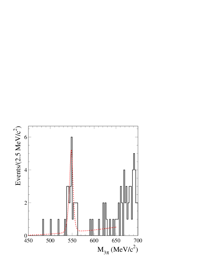
Figure 2: The $3\pi$ invariant mass spectrum for the $e^{+}e^{-}\!\!\to\!\eta\gamma$ candidates in the data. The dashed curve represents the result of the fit described in the text.

To suppress backgrounds in the $e^{+}e^{-}\!\!\to\!\eta\gamma$ sample from events containing kaons and events from multi-particle ISR, QED, and $e^{+}e^{-}\!\to\!q\bar{q}$ processes, while maintaining high signal efficiency, we consider events with exactly one pair of selected tracks and no more than one additional track. Considering the selected pair, we require that: i) neither track is identified as a kaon; ii) $(E_{1}/p_{1})\!+\!(E_{2}/p_{2})\!<\!1.5$, where $E_{i}$ is the EMC energy deposition associated with the $i^{th}$ track and $p_{i}$ is its measured momentum; iii) $\chi^{2}_{2\pi\pi^{0}\gamma}\!\!-\!\chi^{2}_{2\pi 3\gamma}\!<\,$5; and iv) the invariant mass of the two charged tracks $M_{2\pi}\!<\!415~{}{\mathrm{\,Me\kern-1.00006ptV\!/}c^{2}}$. Requirement (ii) suppresses dielectron events; requirement (iv) only suppresses background events with a $\pi^{+}\pi^{-}\pi^{0}$ mass $M_{3\pi}\!>\,$0.6 ${\mathrm{\,Ge\kern-1.00006ptV\!/}c^{2}}$, but it facilitates the extrapolation of the background under the $\eta$ peak.

We show scatter plots of $\chi^{2}_{2\pi\pi^{0}\gamma}$ versus $M_{3\pi}$ for the selected candidates in the data and the $e^{+}e^{-}\!\!\to\!\eta\gamma$ signal simulation in Figs. 1b and 1c. A cluster of data events is evident near the $\eta$ mass at small values of $\chi^{2}_{2\pi\pi^{0}\gamma}$. Figure 2 shows the $M_{3\pi}$ distribution for data events with $\chi^{2}_{2\pi\pi^{0}\gamma}\!<\!20$. In order to determine the number of events containing a true $\eta$ we perform a binned maximum likelihood fit to the $M_{3\pi}$ spectrum over the range 450–650 ${\mathrm{\,Me\kern-1.00006ptV\!/}c^{2}}$ with a sum of signal and background distributions. We describe the signal by a sum of three Gaussian functions with parameters obtained from the simulation, convolved with an additional Gaussian smearing function of width $\sigma_{G}\!=\!1.3^{+0.6}_{-1.0}$ ${\mathrm{\,Me\kern-1.00006ptV\!/}c^{2}}$ determined from high-statistics $\omega\!\!\to\!\pi^{+}\pi^{-}\pi^{0}$ data (see Sec. V). The background is a second order polynomial. The line on Fig. 2 represents the result of the fit. The fitted number of events is $N_{\eta}\!=\!22.7^{+5.6}_{-4.9}\pm 0.6$, where the first error is statistical and the second is the systematic arising from the uncertainty on $\sigma_{G}$, variation of the background parameters, and using a first or third order polynomial background.

Figure 3: Scatter plots of $\chi^{2}_{2\pi\eta\gamma}$ vs. $M_{2\pi\eta}$ for the selected events in the data (top) and $e^{+}e^{-}\!\!\to\!\eta^{\prime}\gamma\!\!\to\!\pi^{+}\pi^{-}\eta\gamma\!\!\to\!\pi^{+}\pi^{-}\gamma\gamma\gamma$ signal simulation (bottom).

For the $e^{+}e^{-}\!\!\to\!\eta^{\prime}\gamma$ reaction in the $\pi^{+}\pi^{-}3\gamma$ final state, we apply the criteria (i)–(ii) above, the analog of (iii) $\chi^{2}_{2\pi\eta\gamma}\!\!-\!\chi^{2}_{2\pi 3\gamma}\!<\,$5, and a slightly different requirement on the two-track mass of $M_{2\pi}\!<\,$410 ${\mathrm{\,Me\kern-1.00006ptV\!/}c^{2}}$, the kinematic limit for the two pions from an $\eta^{\prime}\!\!\to\!\pi^{+}\pi^{-}\eta$ decay. Figure 3 shows scatter plots of $\chi^{2}_{2\pi\eta\gamma}$ versus $M_{2\pi\eta}$ for selected candidates in the data and the $e^{+}e^{-}\!\!\to\!\eta^{\prime}\gamma$ signal simulation; a cluster of data events is evident near the $\eta^{\prime}$ mass at small values of $\chi^{2}_{2\pi\eta\gamma}$. We show the $M_{2\pi\eta}$ spectrum for data events with $\chi^{2}_{2\pi\eta\gamma}\!<\,$20 in Fig. 4, and determine the number of events containing an $\eta^{\prime}$ with a fit to this spectrum similar to that used for the $\eta$ signal, but over the range 900–1000 ${\mathrm{\,Me\kern-1.00006ptV\!/}c^{2}}$. The line on Fig. 4 represents the result of the fit and the fitted number of events is $N_{\eta^{\prime}}\!=\!38.1^{+6.8}_{-6.2}\pm 1.0$.

Figure 4: The $\pi^{+}\pi^{-}\eta$ invariant mass distribution for the $e^{+}e^{-}\!\!\to\!\eta^{\prime}\gamma$ candidates in the data with $\eta^{\prime}\!\!\to\!\pi^{+}\pi^{-}\eta$, $\eta\!\!\to\!\gamma\gamma$. The curve represents the result of the fit described in the text.

For the $e^{+}e^{-}\!\!\to\!\eta^{\prime}\gamma$ reaction in the $4\pi\pi^{0}\gamma$ final state we require $\chi^{2}_{4\pi\pi^{0}\gamma}\!<\!25$ and that none of the four charged tracks is identified as a kaon. We then search for events in which three of the pions are consistent with an $\eta$ decay. Figure 5 shows the distribution of the $\pi^{+}\pi^{-}\pi^{0}$ invariant mass (4 combinations per event) for selected candidates in the data and $e^{+}e^{-}\!\!\to\!\eta^{\prime}\gamma$ signal simulation, with the additional requirement that $M_{5\pi}\!<1$ ${\mathrm{\,Ge\kern-1.00006ptV\!/}c^{2}}$. Peaks at the $\eta$ mass are evident over a modest combinatorial background. We select events with at least one combination in the range 0.535$<M_{3\pi}<$0.56 ${\mathrm{\,Ge\kern-1.00006ptV\!/}c^{2}}$; no event in the data or simulation has more than one. We fit the $5\pi$ invariant mass spectrum for the selected data events as for the other modes, over the range 900–1000 ${\mathrm{\,Me\kern-1.00006ptV\!/}c^{2}}$, and show the distribution and fit result in Fig. 6. The fitted number of events containing a true $\eta^{\prime}$ is $12.0^{+3.9}_{-3.4}\pm 0.3$.

Figure 5: Distributions of $\pi^{+}\pi^{-}\pi^{0}$ invariant mass (4 combinations per event) for selected events in the data (top) and $e^{+}e^{-}\!\!\to\!\eta^{\prime}\gamma\!\!\to\!\pi^{+}\pi^{-}\eta\gamma\!\!\to\!\pi^{+}\pi^{-}\pi^{+}\pi^{-}\pi^{0}\gamma$ simulation (bottom).

Figure 6: The $\pi^{+}\pi^{-}\eta$ invariant mass distribution for the $e^{+}e^{-}\!\!\to\!\eta^{\prime}\gamma$ candidates in the data with $\eta^{\prime}\!\!\to\!\pi^{+}\pi^{-}\eta$, $\eta\!\!\to\!\pi^{+}\pi^{-}\pi^{0}$. The curve represents the result of the fit described in the text.

IV Background

IV.1 $e^{+}e^{-}\to\eta\gamma$

We consider both non-peaking and peaking backgrounds, where the latter arise from other processes producing true $\eta$ mesons or other mesons whose decays reflect or feed down into the $\eta$ mass region. Figure 2 shows that the non-peaking background is small in the $\eta$ mass region, but increases sharply toward the upper edge of the plot. This is due primarily to the low-mass tail of the $\omega$ resonance in the ISR processes $e^{+}e^{-}\!\!\to\!\gamma_{\scriptscriptstyle ISR}\pi^{+}\pi^{-}\pi^{0}$, and $e^{+}e^{-}\!\!\to\!\gamma_{\scriptscriptstyle ISR}\pi^{+}\pi^{-}\pi^{0}\pi^{0}$. Our simulation of these processes is tuned to existing data pdg , and predicts an $M_{3\pi}$ spectrum consistent with our selected data both inside (excluding the $\eta$ peak) and outside the range of Fig. 2. The simulated contributions of other ISR and $e^{+}e^{-}\!\!\to\!q\bar{q}$ processes to the non-peaking background are negligible.

The primary source of peaking background is the set of ISR processes $e^{+}e^{-}\!\!\to\!\gamma_{\scriptscriptstyle ISR}\eta\gamma$, where the $\eta\gamma$ comes from a $\rho$, $\omega$, $\phi$, or $J/\psi$ decay, all of which have been measured. We calculate the number of background events using a simulation based on the vector meson dominance model that includes $\rho$, $\omega$, and $\phi$ amplitudes with PDG resonance parameters pdg and phases of 0^∘, 0^∘, and 180^∘, respectively, and describes the existing data on the $e^{+}e^{-}\!\!\to\!\eta\gamma$ reaction in the $\rho$-$\omega$-$\phi$ mass region SND ; CMD2 . The model also includes $J/\psi$ production, and predicts a total peaking background of 2.6$\pm$0.5 events.

Figure 7: Scatter plot of $\chi^{2}_{3\pi\gamma\gamma}$ versus $M_{3\pi}$ for the selected data events containing an additional photon.

Figure 8: The $3\pi$ invariant mass spectrum for events in the data with $\chi^{2}_{3\pi\gamma\gamma}<25$. The solid vertical lines bound the $\eta$ signal region; the sideband regions are between these and the dashed lines.

The simulation does not include other contributions such as decays of excited $\rho$, $\omega$, or $\phi$ states, as they are unmeasured and expected to be small. As a check, we select $e^{+}e^{-}\!\!\to\!\gamma_{\scriptscriptstyle ISR}\eta\gamma$ events explicitly from our data, by subjecting any event with an additional photon to a kinematic fit to the $3\pi\gamma\gamma$ hypothesis. Figure 7 shows a scatter plot of the $\chi^{2}$ of this fit ($\chi^{2}_{3\pi\gamma\gamma}$) versus the $3\pi$ invariant mass, and Fig. 8 shows the $M_{3\pi}$ spectrum for events with $\chi^{2}_{3\pi\gamma\gamma}\!<\,$25; a strong $\eta$ signal is present. We estimate the number of $e^{+}e^{-}\!\!\to\!\gamma_{\scriptscriptstyle ISR}\eta\gamma$ events by counting the events in the signal region indicated in Fig. 8 and subtracting the number in the two sidebands. The resulting number of events, 274$\pm$22, is consistent with the 261$\pm$5$\pm$9 expected from the simulation, where the systematic error in the latter is due to experimental uncertainties on the input parameters to the simulation. Repeating this exercise in several different ranges of the $\eta\gamma$ invariant mass, we obtain the results listed in Table 1; data and simulation are consistent.

Table 1: The number of selected $e^{+}e^{-}\!\!\to\!\gamma_{\scriptscriptstyle ISR}\eta\gamma$ events in the data in several ranges of the $\eta\gamma$ invariant mass compared with expectations from the simulation. The first error on each expected number is statistical, the second systematic.

$M_{\eta\gamma}$ (GeV/$c^{2})$	$N_{data}$		$N_{expect}$
0.55–0.95	25$\pm$	9	43$\pm$	3 $\pm$	4
0.95–1.05	200$\pm$	15	192$\pm$	5 $\pm$	4
1.05–3.05	18$\pm$	12	5$\pm$	1 $\pm$	6
3.05–3.15	31$\pm$	6	21$\pm$	1 $\pm$	2
3.15–6.50	0.0$\pm$	1.4	1$\pm$	0.4 $\pm$	2
0.55–6.50	274$\pm$	22	261$\pm$	5 $\pm$	9

Other possible sources of peaking background are the processes $e^{+}e^{-}\!\!\to\!VP\!\!\to\!\eta\pi^{0}\gamma$, where $V$ denotes a vector meson, $\rho$, $\omega$, or $\phi$, and $P$ is a $\pi^{0}$ or $\eta$. The CLEO and BES experiments have measured these cross sections at $\sqrt{q^{2}}\approx\,$3.7 $\mathrm{\,Ge\kern-1.00006ptV}$ CLEOVP ; BESVP ; assuming the $1/q^{4}$ dependence of $VP$ form factors predicted by perturbative QCD chernyakPR , we estimate the $e^{+}e^{-}\!\!\to\!\eta\pi^{0}\gamma$ cross section to be about 3 fb at our c.m. energy. The simulated selection efficiency is very low due to the additional $\pi^{0}$, approximately 2$\times\!10^{-4}$, so we expect only 0.2 background events from this source. The corresponding ISR process $e^{+}e^{-}\!\!\to\!\gamma_{\scriptscriptstyle ISR}VP$ can also contribute, and we estimate a cross section of about 13 fb, (for 20${}^{\circ}\!<\!\theta^{\ast}_{\gamma}\!<$160^∘), based on our studies of several ISR final states with $VP$ components BAD767 ; isrrefs , including $4\pi$, $3\pi$, $3\pi\eta$, $2\pi\eta$, $2K\pi^{0}$, and $2K\eta$. This cross section is relatively large, one-quarter of the $e^{+}e^{-}\!\!\to\!\gamma_{\scriptscriptstyle ISR}\eta\gamma$ cross section, but the selection efficiency is less than 2$\times\!10^{-5}$, so we expect no more than 0.1 events from this source.

The $e^{+}e^{-}\!\!\to\!\gamma_{\scriptscriptstyle ISR}\eta\pi^{0}\gamma$ and $e^{+}e^{-}\!\!\to\!\eta\pi^{0}\gamma$ events are selected about 100 times more efficiently by the $\eta\gamma\gamma$ criteria than by the $\eta\gamma$ criteria, and similar factors apply to other types of events containing additional pions and/or photons. We can therefore make another estimate of their overall contribution from the difference between the observed and expected numbers of $e^{+}e^{-}\!\!\to\!\gamma_{\scriptscriptstyle ISR}\eta\gamma$ candidates of 13$\pm$24 (Table 1). Accounting for the $\sim$10% uncertainty in relative selection efficiencies, we estimate $<\,$0.6 such events in our signal peak at the 90% CL.

ISR production of an $\mathchar 28935\relax(1S)$, $\mathchar 28935\relax(2S)$, or $\mathchar 28935\relax(3S)$ resonance could produce a peaking background if the $\mathchar 28935\relax$ decays to $\eta\gamma$, since the ISR photon is rather soft. From the upper limit on ${\cal B}(\mathchar 28935\relax(1S)\!\!\to\!\eta\gamma)$ of 2.1$\times\!10^{-5}$ pdg , we estimate that the number of $e^{+}e^{-}\!\!\to\!\gamma_{\scriptscriptstyle ISR}\mathchar 28935\relax(1S)\!\!\to\!\eta\gamma\gamma$ events in our data does not exceed 100. Using the relation

$$\frac{\Gamma(\mathchar 28935\relax(nS)\to\eta\gamma)}{\Gamma(\mathchar 28935\relax(1S)\to\eta\gamma)}\approx\frac{\Gamma(\mathchar 28935\relax(nS)\to e^{+}e^{-})}{\Gamma(\mathchar 28935\relax(1S)\to e^{+}e^{-})},\;n=2,3$$

we obtain corresponding limits for $\mathchar 28935\relax(2S)$ and $\mathchar 28935\relax(3S)$ of 50 and 140, respectively. The selection efficiencies for the $1S$, $2S$, and $3S$ processes are below 0.01%, 0.02%, and 0.08%, respectively, so the total $\mathchar 28935\relax$ background does not exceed 0.13 events.

We search for peaking background in the $e^{+}e^{-}\!\!\to\!q\overline{q}$ process using the JETSET simulation. From 736 million simulated events (corresponding to about twice our integrated luminosity) only two events pass the $\eta\gamma$ selection criteria. Only one of them, a $K^{0}\overline{K}^{0}\eta$ final state, has a $3\pi$ invariant mass close to the $\eta$ mass. Since we do not expect JETSET to predict rates for such rare events correctly, we select $e^{+}e^{-}\!\!\to\!K\overline{K}\eta$, $\eta\!\!\to\!\gamma\gamma$ events from our data as a check. We perform a kinematic fit to the $K^{+}K^{-}\gamma\gamma$ hypothesis on all events with at least one charged track identified as a kaon, and select events with $\chi^{2}_{2K\gamma\gamma}\!<$10. From the 2$\pm$30 events found in the data and 312$\pm$14 expected from the simulation, we conclude that JETSET overestimates the yield and that this source of background is negligible.

Taking the estimate of the number of peaking background events from $e^{+}e^{-}\!\!\to\!\gamma_{\scriptscriptstyle ISR}\eta\gamma$, and considering the upper limits on all the other sources as additional systematic errors, we estimate the total peaking background to be 2.6$\pm$0.8 events. Subtracting this from the number of observed events with a true $\eta$, we obtain the number of detected $e^{+}e^{-}\!\!\to\!\eta\gamma$ events:

$$N_{\eta\gamma}=20.1^{+5.6}_{-4.9}\pm 1.0.$$

IV.2 $e^{+}e^{-}\to\eta^{\prime}\gamma$

We estimate backgrounds in the $e^{+}e^{-}\!\!\to\!\eta^{\prime}\gamma$ sample using similar procedures. The non-peaking background is very small for both the $\eta\!\to\!\gamma\gamma$ (see Fig. 4) and $\eta\!\to\!\pi^{+}\pi^{-}\pi^{0}$ (see Fig. 6) modes. According to the simulations, it is dominated by the ISR processes $e^{+}e^{-}\!\!\to\!\gamma_{\scriptscriptstyle ISR}\pi^{+}\pi^{-}\pi^{0}$ and $e^{+}e^{-}\!\!\to\!\gamma_{\scriptscriptstyle ISR}\pi^{+}\pi^{-}\pi^{0}\pi^{0}$. As for the $e^{+}e^{-}\!\!\to\!\eta\gamma$ process, the simulated non-peaking background mass distributions are consistent with those observed in data.

The largest source of peaking background in the simulations is the ISR process $e^{+}e^{-}\!\!\to\!\gamma_{\scriptscriptstyle ISR}\eta^{\prime}\gamma$, where the $\eta^{\prime}\gamma$ comes mainly from $\phi$ and $J/\psi$ decays. These have been measured with about 10% accuracy, and we use a vector-dominance based simulation similar to that for the $\eta\gamma$ analysis to estimate their contribution. In addition to the $\phi$ and $J/\psi$, we include contributions from the high-mass tails of the $\rho$ and $\omega$ with couplings determined from the measured $\eta^{\prime}\!\!\to\!\omega\gamma$ and $\rho\gamma$ decay widths. We estimate a peaking background from this source of 0.3$\pm$0.1 events in each of the two $\eta$ decay modes.

We check this prediction by selecting $e^{+}e^{-}\!\!\to\!\gamma_{\scriptscriptstyle ISR}\eta^{\prime}\gamma$ events using a kinematic fit to the $\pi^{+}\pi^{-}\eta\gamma\gamma$ hypothesis. Selecting events with a $\chi^{2}_{2\pi\eta\gamma\gamma}\!<\!25$, we count signal and sideband events in the $\pi^{+}\pi^{-}\eta$ invariant mass distributions to obtain numbers of events from this source in a set of $\eta^{\prime}\gamma$ mass intervals. The results from data and simulation listed in Table 2 are consistent. In the $J/\psi$ mass region these events are practically free of background, and we compare the data and simulated $\pi^{+}\pi^{-}\eta$ invariant mass distributions for events with an $\eta^{\prime}\gamma$ mass in the range 3.05–3.15 ${\mathrm{\,Ge\kern-1.00006ptV\!/}c^{2}}$ in Fig. 9. The RMS of the distribution is 3.9$\pm$0.3 ${\mathrm{\,Me\kern-1.00006ptV\!/}c^{2}}$ in the data and 3.80$\pm$0.06 ${\mathrm{\,Me\kern-1.00006ptV\!/}c^{2}}$ in the simulation.

Table 2: The number of selected $e^{+}e^{-}\!\!\to\!\gamma_{\scriptscriptstyle ISR}\eta^{\prime}\gamma$ events in the data in several ranges of the $\eta^{\prime}\gamma$ invariant mass compared with expectations from simulation. The first error on each expected number is statistical, the second systematic.

$M_{\eta^{\prime}\gamma}$ (GeV/$c^{2})$	$N_{data}$		$N_{expect}$
$<$1.5	$-$2$\pm$	12	1.7$\pm$	0.3 $\pm$	0.2
1.5–2.0	6$\pm$	4	1.0$\pm$	0.2 $\pm$	1.0
2.0–3.0	2$\pm$	3	1.3$\pm$	0.3 $\pm$	1.3
3.0–3.2	97$\pm$	10	102$\pm$	2 $\pm$	10
$>$ 3.2	3$\pm$	3	1.1$\pm$	0.2 $\pm$	1.1
Total	110$\pm$	17	107$\pm$	2 $\pm$	10

Figure 9: Distributions of the $\pi^{+}\pi^{-}\eta$ invariant mass for selected $e^{+}e^{-}\!\!\to\!\gamma_{\scriptscriptstyle ISR}J/\psi\!\!\to\!\gamma_{\scriptscriptstyle ISR}\eta^{\prime}\gamma$ events in the data (points with error bars) and simulation (histogram).

To bound peaking background from $e^{+}e^{-}\!\!\to\!\eta^{\prime}\pi^{0}\gamma$, $e^{+}e^{-}\!\!\to\!\gamma_{\scriptscriptstyle ISR}\eta^{\prime}\pi^{0}\gamma$ and other events containing additional pions and/or photons, we consider the difference between the observed and expected numbers of $e^{+}e^{-}\!\!\to\!\gamma_{\scriptscriptstyle ISR}\eta^{\prime}\gamma$ candidates in Table 2, 3$\pm$20. Taking into account the factor of 30 difference in selection efficiency, along with its 10% systematic uncertainty, we determine that the total background contribution from such processes does not exceed 1 event in the $\eta\!\!\to\!\gamma\gamma$ mode or 0.3 events in the $\eta\!\!\to\!\pi^{+}\pi^{-}\pi^{0}$ mode.

From the upper limit ${\cal B}(\mathchar 28935\relax(1S)\!\!\to\!\eta^{\prime}\gamma)\!<\!1.6\times 10^{-5}$ pdg , we estimate that the number of $e^{+}e^{-}\!\!\to\!\gamma_{\scriptscriptstyle ISR}\mathchar 28935\relax\!\!\to\!\gamma_{\scriptscriptstyle ISR}\eta^{\prime}\gamma$ events in our data does not exceed 80, 40, or 110 for the $1S$, $2S$, or $3S$ states, respectively. The simulated efficiencies for such events to pass the $e^{+}e^{-}\!\!\to\!\eta^{\prime}\gamma$ selection criteria are small, and we estimate that the total $\mathchar 28935\relax$ background does not exceed 0.03 events for the $\eta\!\!\to\!\gamma\gamma$ mode, and is negligible for the $\eta\!\!\to\!\pi^{+}\pi^{-}\pi^{0}$ mode. In the 736 million $e^{+}e^{-}\!\!\to\!q\overline{q}$ events simulated by JETSET, we find none that passes the $\eta^{\prime}\gamma$ selection criteria.

Considering the upper limits as systematic errors, we estimate total peaking backgrounds of 0.3$\pm$1.0 and 0.3$\pm$0.3 events in the $2\pi 3\gamma$ and $4\pi 3\gamma$ final states, respectively. Subtracting these from the numbers of observed $\eta^{\prime}$ events, we obtain a total number of $\eta^{\prime}\gamma$ events,

$$N_{\eta^{\prime}\gamma}=49.5^{+7.7}_{-7.1}\pm 1.5.$$

V Detection efficiency

V.1 $e^{+}e^{-}\to\eta\gamma$

The detection efficiency determined from the simulation is $\varepsilon_{MC}\!=\!(2.01\pm 0.06)\%$, where the error includes a statistical error and the uncertainty in the value of ${\cal B}(\eta\!\to\!\pi^{+}\pi^{-}\pi^{0})$. This efficiency must be corrected to account for deficiencies in the simulated detector response. We take advantage of the relatively large cross section for the ISR process $e^{+}e^{-}\!\!\to\!\gamma_{\scriptscriptstyle ISR}\omega(782)\!\!\to\!\gamma_{\scriptscriptstyle ISR}\pi^{+}\pi^{-}\pi^{0}$, which can be selected with very low background BAD767 . The $M_{3\pi}$ spectrum for this process is described by

$$\frac{{\rm d}N}{{\rm d}M}=\sigma_{3\pi}(M)\frac{{\rm d}L}{{\rm d}M}\,R\,\varepsilon(M),$$ (5)

where $\sigma_{3\pi}(M)$ is the Born cross section for $e^{+}e^{-}\!\!\to\!3\pi$, ${{\rm d}L}/{{\rm dM}}$ is the so-called ISR differential luminosity, $\varepsilon(M)$ is the detection efficiency as a function of mass, and $R$ is a radiative correction factor (see Ref. BAD767, for a more detailed discussion). The $e^{+}e^{-}\!\!\to\!3\pi$ Born cross section near the $\omega$ mass can be described by a Breit-Wigner function with well measured parameters pdg . We calculate the ISR luminosity from the total integrated luminosity $L$ and the theoretical ISR photon radiator function ivanch . The radiative correction factor is known with a theoretical uncertainty below 1% strfun . We can therefore fit the $3\pi$ invariant mass spectrum for events passing the criteria for this analysis in the $\omega$ mass region to determine the efficiency directly from the data.

Figure 10 shows this distribution after subtraction of the $\sim$0.5% background, estimated from simulation as described in Ref. BAD767, . The fitting function is given by Eq.(5) convolved with the simulated detector resolution function. There are three free parameters: the efficiency correction factor $\delta_{\omega}$ ($\varepsilon\!=\!\delta_{\omega}\varepsilon_{MC}$); the $\omega$ mass; and $\sigma_{G}$, an ad-hoc Gaussian smearing to account for any resolution difference between data and simulation. The curve in Fig. 10 represents the result of the fit, which returns:

$$\delta_{\omega} = 0.933\pm 0.009\pm 0.026,$$

$$\sigma_{G} = 1.3^{+0.5}_{-1.0}\pm 0.3{\mathrm{\,Me\kern-1.00006ptV\!/}c^{2}},$$ (6)

where the first error is statistical and the second systematic. The fitted mass is shifted from the nominal value by 0.5 ${\mathrm{\,Me\kern-1.00006ptV\!/}c^{2}}$, consistent with expectations from our detector simulation. The systematic error in the correction factor includes contributions from simulation statistics (1.2%), uncertainties on the radiative correction (1%), background subtraction (0.2%), and the PDG $\omega$ width (1.5%) and peak cross section (1.5%). The systematic error in $\sigma_{G}$ is due to the uncertainty in the $\omega$ width.

Figure 10: The $\pi^{+}\pi^{-}\pi^{0}$ invariant mass spectrum for data events in the $\omega$ mass region. The curve is the result of the fit described in the text.

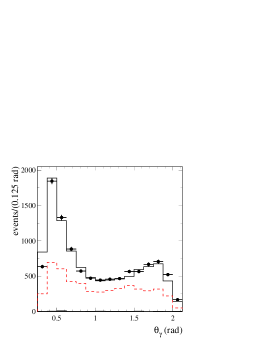
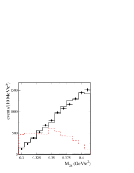
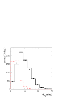
Figure 11: Distributions of the photon polar angle (left), the invariant mass of the two charged pions (middle), and the minimum angle between a charged pion and a photon from the $\pi^{0}$ decay (right) for data (points with error bars) and simulated (solid lines) $e^{+}e^{-}\!\!\to\!\gamma_{\scriptscriptstyle ISR}\omega$ events. The simulated background is shown as the (very small) shaded histograms, and the dashed lines show the distributions for simulated $e^{+}e^{-}\!\!\to\!\eta\gamma$ events.

Figure 12: Distributions of the angle between the two photons from the $\pi^{0}\!\!\to\!\gamma\gamma$ or $\eta\!\to\!\gamma\gamma$ decay (left), and the minimum (middle) and maximum (right) energy of the decay photons, for data (points with error bars) and simulated (solid lines) $e^{+}e^{-}\!\!\to\!\gamma_{\scriptscriptstyle ISR}\omega$ events, simulated background events (small shaded histograms), and simulated $e^{+}e^{-}\!\!\to\!\eta^{\prime}\gamma\!\!\to\!\pi^{+}\pi^{-}\eta$ events (dashed lines).

Before applying this correction to the $e^{+}e^{-}\!\!\to\!\eta\gamma$ efficiency, we must take into account differences in the distributions of any kinematic variables on which the efficiency depends. Of the many variables studied, three show large differences, the photon polar angle $\theta_{\gamma}$, the invariant mass of the two charged pions $M_{2\pi}$, and the minimum angle between a charged pion and a photon from the $\pi^{0}$ decay $\theta_{\pi\gamma}$; in Fig. 11 we compare their distributions in simulated $e^{+}e^{-}\!\!\to\!\gamma_{\scriptscriptstyle ISR}\omega$ events (solid histograms) with those in simulated $e^{+}e^{-}\!\!\to\!\eta\gamma$ events (dashed histograms). The $\theta_{\pi\gamma}$ distribution for the $e^{+}e^{-}\!\!\to\!\gamma_{\scriptscriptstyle ISR}\omega$ data (dots in Fig. 11) is consistent with that for the simulation, but significant inconsistencies are visible in the $\theta_{\gamma}$ ($\chi^{2}/\mbox{dof}=38/14$) and $M_{2\pi}$ ($\chi^{2}/\mbox{dof}=17/11$) distributions. To estimate shifts in the efficiency correction due to the dependence of the efficiency on these variables, we calculate

$$r_{x}=\sum_{i}\frac{P_{\omega}^{exp}(x_{i})}{P_{\omega}^{MC}(x_{i})}{P_{\eta}^{MC}(x_{i})},\;x=\theta_{\gamma},M_{2\pi},$$ (7)

where $P_{\omega(\eta)}$ is the $\theta_{\gamma}$ or $M_{2\pi}$ distribution for $\omega\gamma$ ($\eta\gamma$) events normalized to unit area, and $x_{i}$ is the center of the $i^{\rm th}$ bin. We obtain the values $r_{\theta_{\gamma}}\!=\!1.011\pm 0.006$ and $r_{M_{2\pi}}\!=\!0.973\pm 0.016$, from which we calculate the efficiency correction $\delta_{\eta}\!=\!r_{\theta_{\gamma}}r_{M_{2\pi}}\delta_{\omega}\!=\!0.918\pm 0.032$, and the detection efficiency $\varepsilon\!=\!\delta_{\eta}\varepsilon_{MC}=(1.85\pm 0.09)\%$.

V.2 $e^{+}e^{-}\to\eta^{\prime}\gamma$

The simulated efficiency for $e^{+}e^{-}\!\!\to\!\eta^{\prime}\gamma\!\!\to\!2\pi 3\gamma$ events is $\varepsilon_{MC}\!=\!(2.91\pm 0.13)\%$. For this final state we can again use the efficiency correction determined from the $e^{+}e^{-}\!\to\!\gamma_{\scriptscriptstyle ISR}\omega$ events, taking into account differences in the relevant kinematic variables. Considering the same set of variables, we find similar results: corrections are needed only for $\theta_{\gamma}$ and $M_{2\pi}$ with very similar values of $r_{\theta_{\gamma}}\!=\!1.016\pm 0.008$ and $r_{M_{2\pi}}\!=\!0.976\pm 0.013$. In addition, there are photon distributions that are different for $\pi^{0}$ and $\eta$ decays. We show distributions of the angle between the two decay photons $\theta_{\gamma\gamma}$, and the minimum and maximum photon energies $E_{\gamma,{\rm min}}$ and $E_{\gamma,{\rm max}}$ in Fig. 12. A disagreement between data and simulation for $e^{+}e^{-}\!\!\to\!\gamma_{\scriptscriptstyle ISR}\omega$ events is seen in the $E_{\gamma,{\rm max}}$ spectrum ($\chi^{2}/\mbox{dof}=18/11$) and we calculate $r_{E_{\gamma,{\rm max}}}\!=\!1.035\pm 0.016$. This correction is not needed for $e^{+}e^{-}\!\!\to\!\eta\gamma$ events since their $E_{\gamma,{\rm max}}$ distribution is very close to that for $e^{+}e^{-}\!\!\to\!\gamma_{\scriptscriptstyle ISR}\omega$ events. We calculate an efficiency correction of $\delta_{\eta^{\prime}}\!=\!r_{\theta_{\gamma}}r_{M_{2\pi}}r_{E_{\gamma,{\rm max}}}\delta_{\omega}\!=\!0.957\pm 0.037$, and a detection efficiency of $\varepsilon\!=\!\delta_{\eta^{\prime}}\varepsilon_{MC}\!=\!(2.79\pm 0.16)\%$.

The simulated efficiency for $e^{+}e^{-}\!\!\to\!\eta^{\prime}\gamma\!\!\to\!4\pi 3\gamma$ events is $(1.05\pm 0.07)\%$. We estimate an efficiency correction for the two additional pions using the ISR process $e^{+}e^{-}\!\!\to\!\gamma_{\scriptscriptstyle ISR}\rho\eta\!\!\to\!\pi^{+}\pi^{-}\eta\gamma$. We select events in both the $\eta\!\!\to\!\gamma\gamma$ and $\eta\!\!\to\!\pi^{+}\pi^{-}\pi^{0}$ decay modes with criteria similar to those used for the signal. The $\pi^{+}\pi^{-}\eta$ invariant mass must be in the range 1.4–1.7 ${\mathrm{\,Ge\kern-1.00006ptV\!/}c^{2}}$ where the $\rho\eta$ mass spectrum is at a maximum, and the invariant mass of the $\rho$ candidate must be in the range 0.64–0.90 ${\mathrm{\,Ge\kern-1.00006ptV\!/}c^{2}}$. From the numbers of selected data and simulated events in the two $\eta$ decay modes we determine the double ratio $\delta_{5\pi}\!=\!(N_{3\pi}/N_{2\gamma})_{data}/(N_{3\pi}/N_{2\gamma})_{MC}\!=\!0.98\pm$0.06, and we calculate a fully corrected detection efficiency of $\varepsilon\!=\!\delta_{5\pi}\delta_{\eta^{\prime}}\varepsilon_{MC}\!=(0.99\pm 0.10)\%$. The ratio of the numbers of events selected in the two decay modes, 0.31$\pm$0.11, is consistent with the ratio of simulated detection efficiencies 0.35$\pm$0.04. The total detection efficiency for the two modes is $(3.78\pm 0.19)\%$.

VI Cross sections and form factors

For each of the two signal processes, we calculate the cross section as

$$\sigma(e^{+}e^{-}\to P\gamma)=\frac{N_{P\gamma}}{\varepsilon L}R,$$ (8)

where $N_{P\gamma}$ is the number of signal events from Sec. IV, $\varepsilon$ is the detection efficiency from Sec. V, $L\!=$232 fb^-1 is the integrated luminosity, and $R$ is a radiative correction factor. We calculate $R$ as the ratio of the Born cross section for $e^{+}e^{-}\!\!\to\!P\gamma$ to the total cross section including higher-order radiative corrections calculated with the structure function method strfun . The simulation requires the invariant mass of the $P\gamma$ system $M_{P\gamma}\!>\,$8 ${\mathrm{\,Ge\kern-1.00006ptV\!/}c^{2}}$, for which we calculate $R\!=\,$0.956. The detection efficiency used in Eq.(8) is for simulated events with this requirement. The value of $R$ depends on the energy dependence of the cross section. We use $\sigma\propto 1/q^{4}$ (see Eqs. (1) and (2)), and investigate the model dependence by recalculating $R/\varepsilon$ under the $1/q^{3}$ and $1/q^{5}$ hypotheses. The relative variation is less than $10^{-3}$, which we neglect. The theoretical uncertainty on $R$ obtained with the structure function method does not exceed 1%. We obtain

$$\sigma(e^{+}e^{-}\to\eta\gamma) = 4.5^{+1.2}_{-1.1}\pm 0.3\mbox{ fb},$$ (9)

$$\sigma(e^{+}e^{-}\to\eta^{\prime}\gamma) = 5.4\pm 0.8\pm 0.3\mbox{ fb},$$ (10)

where the first error is statistical and the second systematic. The systematic error is the sum in quadrature of contributions from detection efficiency, background subtraction, fitting procedure, and radiative correction.

The value of $R$ we use does not take into account vacuum polarization, and its contribution is included in the results (9)–(10). For comparison with theoretical predictions, we calculate the so-called “undressed” cross section by applying a 7.5$\pm$0.2% correction for vacuum polarization at 10.58 ${\mathrm{\,Ge\kern-1.00006ptV\!/}c^{2}}$ vp , obtaining

$$\sigma(e^{+}e^{-}\to\eta\gamma)_{\rm undressed} = 4.2^{+1.2}_{-1.0}\pm 0.3\mbox{ fb},$$ (11)

$$\sigma(e^{+}e^{-}\to\eta^{\prime}\gamma)_{\rm undressed} = 5.0^{+0.8}_{-0.7}\pm 0.3\mbox{ fb}.$$ (12)

Using Eq.(1) we obtain the values of the $\eta\gamma$ and $\eta^{\prime}\gamma$ transition form factors at $q^{2}=$112$\mathrm{\,Ge\kern-1.00006ptV}^{2}$

$$q^{2}|F_{\eta}(q^{2})| = 0.229\pm 0.030\pm 0.008\mathrm{\,Ge\kern-1.00006ptV},$$ (13)

$$q^{2}|F_{\eta^{\prime}}(q^{2})| = 0.251\pm 0.019\pm 0.008\mathrm{\,Ge\kern-1.00006ptV}.$$ (14)

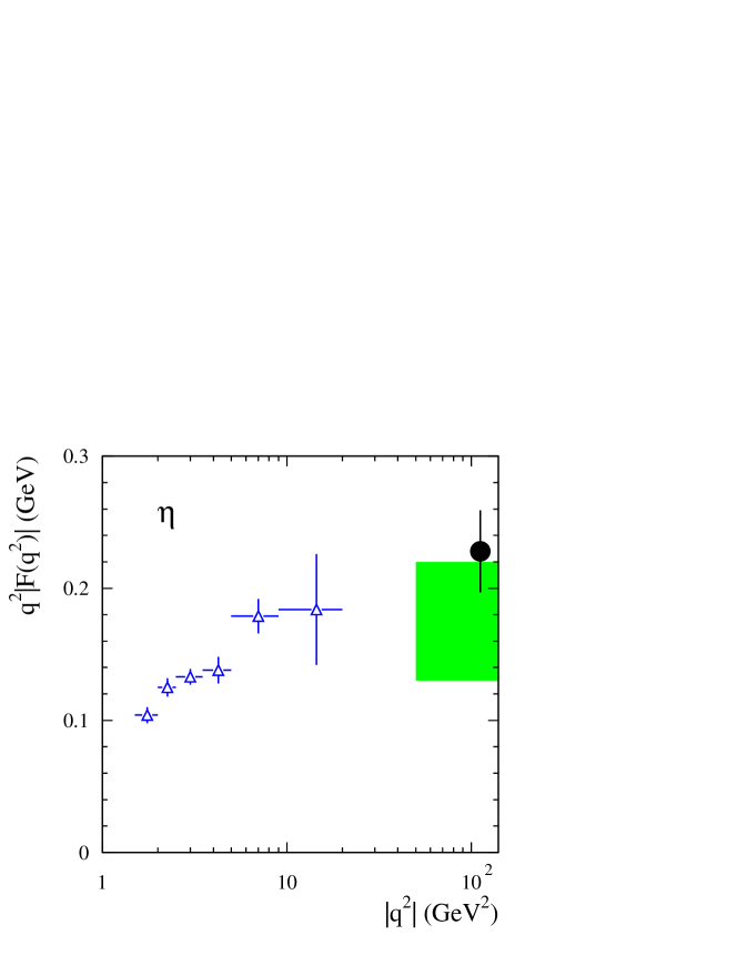
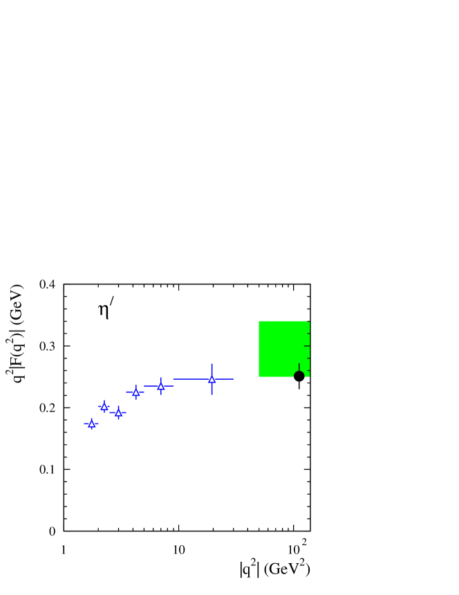
Figure 13: The magnitudes of the $\eta\gamma$ (top) and $\eta^{\prime}\gamma$ (bottom) transition form factors measured in this work (filled circle) and by CLEO CLEO97 (triangles). The shaded boxes indicate the ranges of form-factor values calculated according to Eq.(2) with the decay constants from Refs. Feldman ; Kaiser ; Benayoun ; Goity ; DeFazio ; Escribano .

VII Summary

We have studied the $e^{+}e^{-}\!\!\to\!\eta\gamma$ and $e^{+}e^{-}\!\!\to\!\eta^{\prime}\gamma$ processes at an $e^{+}e^{-}$ c.m. energy of 10.58 GeV. We select $20^{+6}_{-5}$ $\eta\gamma$ and $50^{+8}_{-7}$ $\eta^{\prime}\gamma$ events, measure the cross sections and extract the values of the transition form factors at $q^{2}\!=\!112~{}\mathrm{\,Ge\kern-1.00006ptV}^{2}$.

Since the asymptotic values of the time-like and space-like transition form factors are expected to be very close, we show our results along with CLEO results for space-like momentum transfers CLEO97 in Fig. 13 (we averaged the CLEO results obtained in different $\eta$ ($\eta^{\prime}$) decay modes). The CLEO data rise with increasing $q^{2}$, and are consistent with the values given by our data points. A precise theoretical prediction of the value of the form factor at $q^{2}\!=\!112~{}\mathrm{\,Ge\kern-1.00006ptV}^{2}$ is problematic due to uncertainties in the effective decay constants, the quark distribution amplitudes, and possible gluon content of the $\eta$ and $\eta^{\prime}$. Naively taking the decay constants from Refs. Feldman ; Kaiser ; Benayoun ; Goity ; DeFazio ; Escribano and calculating form factor values according to Eq.(2), we obtain a range of values indicated by the shaded boxes in Fig. 13. Our data points are at the upper and lower ends of the range of predictions for $\eta$ and $\eta^{\prime}$, respectively. The predicted ratio of the form factors ranges from 1.6 to 2.3, inconsistent with our value of $1.10\pm 0.17$. This discrepancy and the large range of the predictions indicates the need for more theoretical input.

VIII Acknowledgments

We thank V.L. Chernyak, A.I. Milstein and Z.K. Silagadze for many fruitful discussions. We are grateful for the extraordinary contributions of our PEP-II colleagues in achieving the excellent luminosity and machine conditions that have made this work possible. The success of this project also relies critically on the expertise and dedication of the computing organizations that support BABAR. The collaborating institutions wish to thank SLAC for its support and the kind hospitality extended to them. This work is supported by the US Department of Energy and National Science Foundation, the Natural Sciences and Engineering Research Council (Canada), Institute of High Energy Physics (China), the Commissariat à l’Energie Atomique and Institut National de Physique Nucléaire et de Physique des Particules (France), the Bundesministerium für Bildung und Forschung and Deutsche Forschungsgemeinschaft (Germany), the Istituto Nazionale di Fisica Nucleare (Italy), the Foundation for Fundamental Research on Matter (The Netherlands), the Research Council of Norway, the Ministry of Science and Technology of the Russian Federation, and the Particle Physics and Astronomy Research Council (United Kingdom). Individuals have received support from CONACyT (Mexico), the Marie-Curie Intra European Fellowship program (European Union), the A. P. Sloan Foundation, the Research Corporation, and the Alexander von Humboldt Foundation.

References

(1)
G.P. Lepage and S.J. Brodsky, Phys. Rev. D 22, 2157 (1980).
(2)
E. Braaten. Phys. Rev. D 28, 524 (1983).
(3)
T. Feldmann, P. Kroll, B. Stech, Phys. Rev. D 58, 114006 (1998).
(4)
H. Leutwyler, Nucl. Phys. Proc. Suppl. 64, 223 (1998).
(5)
M. Benayoun, L. DelBuono and H. B. O’Connell,
Eur. Phys. J. C 17, 593 (2000).
(6)
J. L. Goity, A. M. Bernstein and B. R. Holstein,
Phys. Rev. D 66, 076014 (2002).
(7)
F. De Fazio and M. R. Pennington,
JHEP 0007, 051 (2000).
(8)
R. Escribano and J. M. Frere,
JHEP 0506, 029 (2005).
(9)
P. Kroll, Mod. Phys. Lett. A 20, 2667 (2005).
(10)
M.N. Achasov et al. (SND Collaboration),
JETP Lett. 72, 282 (2000).
(11)
R.R. Akhmetshin et al. (CMD-2 Collaboration),
Phys. Lett. B 509, 72 (2001).
(12)
Review of Particle Physics,
S. Eidelman et al., Phys. Lett. B 592, 1 (2004).
(13)
J. Gronberg et al. (CLEO Collaboration),
Phys. Rev. D 57, 33 (1998).
(14)
M. Acciarri et al. (L3 Collaboration),
Phys. Lett. B 418, 399 (1998).
(15)
H. J. Behrend et al. (CELLO Collaboration),
Z. Phys. C 49, 401 (1991).
(16)
H. Aihara et al. (TPC/2 Collaboration),
Phys. Rev. Lett. 64, 172 (1990).
(17)
C. Berger et al. (PLUTO Collaboration),
Phys. Lett. B 142, 125 (1984).
(18)
V.L. Chernyak, private communication.
(19)
B. Aubert et al. (BABAR Collaboration),
Nucl. Instr. Methods Phys. Res., Sect. A 479, 1 (2002).
(20)
G. Bonneau and F. Martin, Nucl. Phys. B 27, 381 (1971).
(21)
H. Czyż and J.H. Kühn, Eur. Phys. J. C 18, 497 (2001).
(22)
M. Caffo, H. Czyż, and E. Remiddi, Nuo. Cim. 110A, 515 (1997);
Phys. Lett. B 327, 369 (1994).
(23)
T. Sjöstrand, Comput. Phys. Commun. 82, 74 (1994).
(24)
S. Agostinelli et al.,
Nucl. Instr. Methods Phys. Res., Sect. A 506, 250 (2003).
(25)
N.E. Adam et al. (CLEO Collaboration),
Phys. Rev. Lett. 94, 012005 (2005).
(26)
M. Ablikim et al. (BES Collaboration), Phys. Rev. D 70, 112007 (2004);
Erratum-ibid. D 71, 019901 (2005).