Measurement of $\phi_{3}$ with Dalitz Plot Analysis of $B^{+}\to D^{(*)}K^{(*)+}$ Decay

Abstract

We present a measurement of the unitarity triangle angle $\phi_{3}$ using a Dalitz plot analysis of the $K^{0}_{S}\pi^{+}\pi^{-}$ decay of the neutral $D$ meson from the $B^{\pm}\to D^{(*)}K^{(*)\pm}$ process. The method employs the interference between $D^{0}$ and $\overline{D}{}^{0}$ to extract the angle $\phi_{3}$, strong phase $\delta$ and the ratio $r$ of suppressed and allowed amplitudes. We apply this method to a 357 fb^-1 data sample collected by the Belle experiment. The analysis uses three modes: $B^{+}\to DK^{+}$, $B^{+}\to D^{*}K^{+}$ with $D^{*}\to D\pi^{0}$, and $B^{+}\to DK^{*+}$ with $K^{*+}\to K^{0}_{S}\pi^{+}$, as well as the corresponding charge-conjugate modes. From a combined maximum likelihood fit to the three modes, we obtain $\phi_{3}=53^{\circ}\;{}^{+15^{\circ}}_{-18^{\circ}}\mbox{(stat)}\pm 3^{\circ}\mbox{(syst)}\pm 9^{\circ}(\mbox{model})$. The corresponding two standard deviation interval is $8^{\circ}<\phi_{3}<111^{\circ}$.

I Introduction

Determinations of the Cabibbo-Kobayashi-Maskawa (CKM) ckm matrix elements provide important checks on the consistency of the standard model and ways to search for new physics. The possibility of observing direct $CP$ violation in $B\to DK$ decays was first discussed by I. Bigi, A. Carter and A. Sanda bigi . Since then, various methods using $CP$ violation in $B\to DK$ decays have been proposed glw ; dunietz ; eilam ; ads to measure the unitarity triangle angle $\phi_{3}$. These methods are based on two key observations: neutral $D^{0}$ and $\overline{D}{}^{0}$ mesons can decay to a common final state, and the decay $B^{+}\to DK^{+}$ can produce neutral $D$ mesons of both flavors via $\bar{b}\to\bar{c}u\bar{s}$ and $\bar{b}\to\bar{u}c\bar{s}$ transitions, with a relative phase $\theta_{+}$ between the two interfering amplitudes that is the sum, $\delta+\phi_{3}$, of strong and weak interaction phases. For the decay $B^{-}\to DK^{-}$, the relative phase is $\theta_{-}=\delta-\phi_{3}$, so both phases can be extracted from measurements of such charge conjugate $B$ decay modes. However, the use of branching fractions alone requires additional information to obtain $\phi_{3}$. This is provided either by determining the branching fractions of decays to flavour eigenstates (GLW method glw ) or by using different neutral $D$ final states (ADS method ads ).

A Dalitz plot analysis of a three-body final state of the $D$ meson allows one to obtain all the information required for determination of $\phi_{3}$ in a single decay mode. The use of a Dalitz plot analysis for the extraction of $\phi_{3}$ was first discussed by D. Atwood, I. Dunietz and A. Soni, in the context of the ADS method ads . This technique uses the interference of Cabibbo-favored $D^{0}\to K^{-}\pi^{+}\pi^{0}$ and doubly Cabibbo-suppressed $\overline{D}{}^{0}\to K^{-}\pi^{+}\pi^{0}$ decays. However, the small rate for the doubly Cabibbo-suppressed decay limits the sensitivity of this technique.

Three body final states such as $K^{0}_{S}\pi^{+}\pi^{-}$ giri ; binp_dalitz have been suggested as promising modes for the extraction of $\phi_{3}$. In the Wolfenstein parameterization of the CKM matrix elements, the weak parts of the amplitudes that contribute to the decay $B^{+}\to DK^{+}$ are given by $V_{cb}^{*}V_{us\vphantom{b}}^{\vphantom{*}}\sim A\lambda^{3}$ (for the $\overline{D}{}^{0}K^{+}$ final state) and $V_{ub}^{*}V_{cs\vphantom{b}}^{\vphantom{*}}\sim A\lambda^{3}(\rho+i\eta)$ (for $D^{0}K^{+}$). The two amplitudes interfere as the $D^{0}$ and $\overline{D}{}^{0}$ mesons decay into the same final state $K^{0}_{S}\pi^{+}\pi^{-}$; we denote the admixed state as $\tilde{D}_{+}$. Assuming no $CP$ asymmetry in neutral $D$ decays, the amplitude of the $\tilde{D}_{+}$ decay as a function of Dalitz plot variables $m^{2}_{+}=m^{2}_{K^{0}_{S}\pi^{+}}$ and $m^{2}_{-}=m^{2}_{K^{0}_{S}\pi^{-}}$ is

$$M_{+}=f(m^{2}_{+},m^{2}_{-})+re^{i\phi_{3}+i\delta}f(m^{2}_{-},m^{2}_{+}),$$ (1)

where $f(m^{2}_{+},m^{2}_{-})$ is the amplitude of the $\overline{D}{}^{0}\to K^{0}_{S}\pi^{+}\pi^{-}$ decay, and $r$ is the ratio of the magnitudes of the two interfering amplitudes. The value of $r$ is given by the ratio of the CKM matrix elements $|V_{ub}^{*}V_{cs\vphantom{b}}^{\vphantom{*}}|/|V_{cb}^{*}V_{us\vphantom{b}}^{\vphantom{*}}|\sim 0.38$ and the color suppression factor, and is estimated to be in the range 0.1–0.2 gronau .

Similarly, the amplitude of the $\tilde{D}_{-}$ decay from $B^{-}\to DK^{-}$ process is

$$M_{-}=f(m^{2}_{-},m^{2}_{+})+re^{-i\phi_{3}+i\delta}f(m^{2}_{+},m^{2}_{-}).$$ (2)

The $\overline{D}{}^{0}\to K^{0}_{S}\pi^{+}\pi^{-}$ decay amplitude $f$ can be determined from a large sample of flavor-tagged $\overline{D}{}^{0}\to K^{0}_{S}\pi^{+}\pi^{-}$ decays produced in continuum $e^{+}e^{-}$ annihilation. Once $f$ is known, a simultaneous fit of $B^{+}$ and $B^{-}$ data allows the contributions of $r$, $\phi_{3}$ and $\delta$ to be separated. The method has a two-fold ambiguity: $(\phi_{3},\delta)$ and $(\phi_{3}+180^{\circ},\delta+180^{\circ})$ solutions cannot be separated. We always choose the solution with $0<\phi_{3}<180^{\circ}$. References giri and belle_phi3_2 give a more detailed description of the technique.

The method described above can be applied to other modes as well as $B^{+}\to DK^{+}$ decay and its charge-conjugate mode (charge conjugate states are implied throughout the paper). Excited states of neutral $D$ and $K$ mesons can also be used, although the values of $\delta$ and $r$ can differ for these decays. Previously the Belle belle_phi3_2 ; belle_phi3_3 and BaBar babar_phi3_2 collaborations performed analyses using this technique for $B^{+}\to DK^{+}$ and $B^{+}\to D^{*}K^{+}$ decays. Both Belle belle_phi3_bdks and BaBar babar_phi3_bdks have also performed analyses of the $B^{+}\to DK^{*+}$ mode, but the Belle result was not combined with that from the $B^{+}\to D^{(*)}K^{+}$ modes. The latest Belle analyses belle_phi3_3 ; belle_phi3_bdks were based on a 253 fb^-1 data sample. In the current paper, we report a measurement of $\phi_{3}$ with the combination of $B^{+}\to DK^{+}$, $B^{+}\to D^{*}K^{+}$ and $B^{+}\to DK^{*+}$ modes based on a 357 fb^-1 data sample. This analysis supersedes previous Belle results on $\phi_{3}$ using Dalitz plot analysis of $B^{+}\to D^{(*)}K^{(*)+}$ decays.

II Event selection

We use a 357 fb^-1 data sample, corresponding to $386\times 10^{6}$ $B\bar{B}$ pairs, collected by the Belle detector. The decay chains $B^{+}\to DK^{+}$, $B^{+}\to D^{*}K^{+}$ with $D^{*}\to D\pi^{0}$ and $B^{+}\to DK^{*+}$ with $K^{*+}\to K^{0}_{S}\pi^{+}$ are selected for the analysis; the decays $B^{+}\to D\pi^{+}$, $B^{+}\to D^{*}\pi^{+}$ with $D^{*}\to D\pi^{0}$ and $\overline{B}{}^{0}\to D^{*+}\pi^{-}$ with $D^{*+}\to D\pi^{+}$ serve as control samples. The neutral $D$ meson is reconstructed in the $K^{0}_{S}\pi^{+}\pi^{-}$ final state in all cases. We also select decays of $D^{*-}\to\overline{D}{}^{0}\pi^{-}$ produced via the $e^{+}e^{-}\to c\bar{c}$ continuum process as a high-statistics sample to determine the $\overline{D}{}^{0}\to K^{0}_{S}\pi^{+}\pi^{-}$ decay amplitude.

The Belle detector is described in detail elsewhere belle ; svd2 . It is a large-solid-angle magnetic spectrometer consisting of a silicon vertex detector (SVD), a 50-layer central drift chamber (CDC) for charged particle tracking and specific ionization measurement ($dE/dx$), an array of aerogel threshold Čerenkov counters (ACC), time-of-flight scintillation counters (TOF), and an array of CsI(Tl) crystals for electromagnetic calorimetry (ECL) located inside a superconducting solenoid coil that provides a 1.5 T magnetic field. An iron flux return located outside the coil is instrumented to detect $K_{L}$ mesons and identify muons (KLM).

Charged tracks are required to satisfy criteria based on the quality of the track fit and the distance from the interaction point in both longitudinal and transverse planes with respect to the beam axis. To reduce the low momentum combinatorial background we require each track to have a transverse momentum greater than 100 MeV/$c$. Separation of kaons and pions is accomplished by combining the responses of the ACC and the TOF with the $dE/dx$ measurement from the CDC to form a likelihood $\mathcal{L}(h)$ where $h$ is a pion or a kaon. Charged particles are identified as pions or kaons using the likelihood ratio $\mathcal{R}_{\rm PID}(h)=\mathcal{L}(h)/(\mathcal{L}(K)+\mathcal{L}(\pi))$. For charged kaon identification, we require $\mathcal{R}_{\rm PID}(K)>0.7$. This requirement selects kaons with an efficiency of 80% and pions with an efficiency of 5%.

Photon candidates are required to have ECL energy greater than 30 MeV. Neutral pion candidates are formed from pairs of photons with invariant masses in the range 120 to 150 MeV/$c^{2}$, i.e. less than two standard deviations from the $\pi^{0}$ mass.

Neutral kaons are reconstructed from pairs of oppositely charged tracks without any pion PID requirement. We require the reconstructed vertex distance from the interaction point in the plane transverse to the beam axis to be more than 1 mm and the invariant mass $M_{\pi\pi}$ to satisfy $|M_{\pi\pi}-M_{K^{0}_{S}}|<10$ MeV/$c^{2}$, i.e. less than four standard deviations from the nominal $K^{0}_{S}$ mass.

II.1 Selection of $D^{*-}\to\overline{D}{}^{0}\pi^{-}$

To determine the $\overline{D}{}^{0}\to K^{0}_{S}\pi^{+}\pi^{-}$ decay amplitude we use $D^{*\pm}$ mesons produced via the $e^{+}e^{-}\to c\bar{c}$ continuum process. The flavor of the neutral $D$ meson is tagged by the charge of the slow pion (which we denote as $\pi_{s}$) in the decay $D^{*-}\to\overline{D}{}^{0}\pi_{s}^{-}$.

To select neutral $D$ candidates we require the invariant mass of the $K^{0}_{S}\pi^{+}\pi^{-}$ system to be within 9 MeV/$c^{2}$ of the $D^{0}$ mass, $M_{D^{0}}$. To select events originating from a $D^{*-}$ decay we impose a requirement on the difference $\Delta M=M_{K^{0}_{S}\pi^{+}\pi^{-}\pi_{s}}-M_{K^{0}_{S}\pi^{+}\pi^{-}}$ of the invariant masses of the $D^{*-}$ and the neutral $D$ candidates: $144.6\mbox{ MeV}/c^{2}<\Delta M<146.4\mbox{ MeV}/c^{2}$. The resolutions of the selection variables are $\sigma(\Delta M)=0.38$ MeV$/c^{2}$ and $\sigma(M_{K^{0}_{S}\pi^{+}\pi^{-}})=5.4$ MeV$/c^{2}$. The suppression of the combinatorial background from $B\bar{B}$ events is achieved by requiring the $D^{*-}$ momentum in the center-of-mass (CM) frame to be greater than 2.7 GeV/$c$.

The number of events that pass all selection criteria is 271621. To obtain the number of background events in our sample we fit the $\Delta M$ distribution. The background is parameterized with the function $b(\Delta M)\sim(1/\Delta M)\sqrt{(\Delta M/m_{\pi})^{2}-1}$; the function describing the signal is a combination of two Gaussian peaks with the same mean value. The fit finds $(261.9\pm 1.1)\times 10^{3}$ signal events and $8698\pm 77$ background events corresponding to a background fraction of 3.2%.

II.2 Selection of $B^{+}\to DK^{+}$

The selection of $B$ candidates is based on the CM energy difference $\Delta E=\sum E_{i}-E_{\rm beam}$ and the beam-constrained $B$ meson mass $M_{\rm bc}=\sqrt{E_{\rm beam}^{2}-(\sum p_{i})^{2}}$, where $E_{\rm beam}$ is the CM beam energy, and $E_{i}$ and $p_{i}$ are the CM energies and momenta of the $B$ candidate decay products. We select events with $M_{\rm bc}>5.2$ GeV/$c^{2}$ and $|\Delta E|<0.2$ GeV for the analysis. In addition, we impose a requirement on the invariant mass of the neutral $D$ candidate: $|M_{K^{0}_{S}\pi^{+}\pi^{-}}-M_{D^{0}}|<11$ MeV/$c^{2}$.

To suppress background from $e^{+}e^{-}\to q\bar{q}$ ($q=u,d,s,c$) continuum events, we require $|\cos\theta_{\rm thr}|<0.8$, where $\theta_{\rm thr}$ is the angle between the thrust axis of the $B$ candidate daughters and that of the rest of the event. For additional background rejection, we use a Fisher discriminant composed of 11 parameters fisher : the production angle of the $B$ candidate, the angle of the $B$ thrust axis relative to the beam axis and nine parameters representing the momentum flow in the event relative to the $B$ thrust axis in the CM frame. We apply a requirement on the Fisher discriminant that retains 90% of the signal and rejects 40% of the remaining continuum background.

The $\Delta E$ and $M_{\rm bc}$ distributions for $B^{+}\to DK^{+}$ candidates are shown in Fig. 1a,b. The peak in the $\Delta E$ distribution at $\Delta E=50$ MeV is due to $B^{+}\to D\pi^{+}$ decays where the pion is misidentified as a kaon. The $B^{+}\to DK^{+}$ selection efficiency (11%) is determined from a Monte Carlo (MC) simulation. The number of events in the signal box ($|\Delta E|<30$ MeV, $5.27$ GeV/$c^{2}<M_{\rm bc}<5.3$ GeV/$c^{2}$) is 470.

For the selected events a two-dimensional unbinned maximum likelihood fit in the variables $M_{\rm bc}$ and $\Delta E$ is performed. The resulting signal and background density functions are used in the Dalitz plot fit to obtain the event-by-event signal to background ratio. To parametrize the shape of the $\Delta E-M_{\rm bc}$ distribution, we use two-dimensional Gaussian peaks for the signal contribution and $B^{+}\to D\pi^{+}$ background. The non-peaking background is parametrized by the sum of two components: the product of an empirical shape introduced by ARGUS argus as a function of $M_{\rm bc}$ and a linear function in $\Delta E$, and the product of a Gaussian distribution in $M_{\rm bc}$ and a linear function in $\Delta E$. Only the region with $\Delta E>-0.1$ GeV is used in the fit; the region with $\Delta E<-0.1$ GeV includes a large fraction of events from $B\to D^{*}K$ decay with a lost pion that do not contribute to the signal box. The number of events in the signal peak obtained from the fit is $331\pm 23$; the event purity in the signal box is 67%.

II.3 Selection of $B^{+}\to D^{*}K^{+}$

For the selection of $B^{+}\to D^{*}K^{+}$ events, in addition to the requirements described above, we require that the mass difference $\Delta M=M_{K^{0}_{S}\pi^{+}\pi^{-}\pi^{0}}-M_{K^{0}_{S}\pi^{+}\pi^{-}}$ of neutral $D^{*}$ and $D$ candidates satisfies $140\mbox{ MeV}/c^{2}<\Delta M<145\mbox{ MeV}/c^{2}$. Figures 1c,d show the $\Delta E$ and $M_{\rm bc}$ distributions for $B^{+}\to D^{*}K^{+}$ candidates. The selection efficiency is 6.2%. The number of events in the signal box is 111. The parametrization of background and signal shapes is similar to that in the $B^{+}\to DK^{+}$ case. The number of events in the signal peak obtained from the fit is $81\pm 11$; the event purity in the signal box is 77%.

II.4 Selection of $B^{+}\to DK^{*+}$

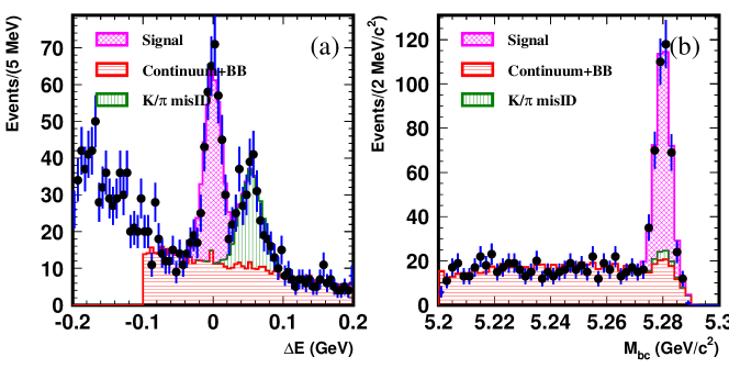
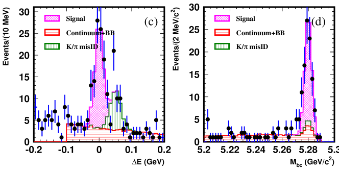
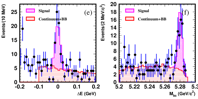
Figure 1: $\Delta E$ and $M_{\rm bc}$ distributions for the (a,b) $B^{+}\to DK^{+}$, (c,d) $B^{+}\to D^{*}K^{+}$, and (e,f) $B^{+}\to DK^{*+}$ event samples. Points with error bars are the data, and the histogram is the result of a MC simulation according to the fit result.

For $B^{+}\to DK^{*+}$ decay candidates, in addition to the requirements placed on the $B^{+}\to DK^{+}$ mode, $K^{*+}$ candidate selection is performed. To select $K^{*+}$ meson candidates, we require the $K^{0}_{S}\pi^{+}$ invariant mass to be within 50 MeV/$c^{2}$ of the $K^{*+}$ nominal mass. For continuum background suppression, in addition to the $|\cos\theta_{\rm thr}|<0.8$ condition, we require that the $K^{*+}$ helicity angle satisfy $|\cos\theta_{\rm hel}|>0.4$. The $K^{*+}$ helicity angle is defined as the angle between the axis of the $K^{*+}$ decay products, and the momentum of the $B$ meson, in the $K^{*+}$ rest frame. We also apply a requirement on the Fisher discriminant that retains 95% of the signal and rejects 30% of the remaining continuum background. Figures 1e,f show the $\Delta E$ and $M_{\rm bc}$ distributions for $B^{+}\to DK^{*+}$ candidates. The selection efficiency is 4.1%. The number of events in the signal box is 78. The parametrization of background and signal shapes is similar to that in the $B^{+}\to DK^{+}$ case, but without the contribution of $K/\pi$ misidentification background. The number of events in the signal peak obtained from the fit is $54\pm 8$; the event purity in the signal box is 65%.

III Determination of the $\overline{D}{}^{0}\to K^{0}_{S}\pi^{+}\pi^{-}$ decay amplitude

The amplitude $f$ for the $\overline{D}{}^{0}\to K^{0}_{S}\pi^{+}\pi^{-}$ decay is described by a coherent sum of two-body decay amplitudes and one non-resonant decay amplitude,

$$f(m^{2}_{+},m^{2}_{-})=\sum\limits_{j=1}^{N}a_{j}e^{i\alpha_{j}}\mathcal{A}_{j}(m^{2}_{+},m^{2}_{-})+be^{i\beta},$$ (3)

where $N$ is the total number of resonances, $\mathcal{A}_{j}(m^{2}_{+},m^{2}_{-})$ is the matrix element, $a_{j}$ and $\alpha_{j}$ are the amplitude and phase of the matrix element, respectively, of the $j$-th resonance, and $b$ and $\beta$ are the amplitude and phase of the non-resonant component. The total phase and amplitude are arbitrary. To be consistent with other analyses babar_phi3_2 ; dkpp_cleo we have chosen the $\overline{D}{}^{0}\to K^{0}_{S}\rho$ mode to have unit amplitude and zero relative phase. The description of the matrix elements follows Ref. cleo_model .

We use a set of 18 two-body amplitudes. These include five Cabibbo-allowed amplitudes: $K^{*}(892)^{+}\pi^{-}$, $K^{*}(1410)^{+}\pi^{-}$, $K_{0}^{*}(1430)^{+}\pi^{-}$, $K_{2}^{*}(1430)^{+}\pi^{-}$ and $K^{*}(1680)^{+}\pi^{-}$; their doubly Cabibbo-suppressed partners; and eight amplitudes with $K^{0}_{S}$ and a $\pi\pi$ resonance: $K^{0}_{S}\rho$, $K^{0}_{S}\omega$, $K^{0}_{S}f_{0}(980)$, $K^{0}_{S}f_{2}(1270)$, $K^{0}_{S}f_{0}(1370)$, $K^{0}_{S}\rho(1450)$, $K^{0}_{S}\sigma_{1}$ and $K^{0}_{S}\sigma_{2}$. The differences from our previous publication belle_phi3_2 are, i) the addition of $K^{0}_{S}\rho(1450)$, $K^{*}(1410)^{+}\pi^{-}$ and the corresponding doubly Cabibbo-suppressed mode, ii) the use of the Gounaris-Sakurai gounaris amplitude description for the $K^{0}_{S}\rho$ and $K^{0}_{S}\rho(1450)$ contributions, and iii) the mass and width for the $f_{0}(1370)$ state are now taken from Ref. aitala ($M=1434$ MeV$/c^{2}$, $\Gamma=173$ MeV$/c^{2}$).

We use an unbinned maximum likelihood technique to fit the Dalitz plot distribution to the model described by Eq. 3. We minimize the negative logarithm of the likelihood function in the form

$$-2\log L=-2\left[\sum\limits^{n}_{i=1}\log p(m^{2}_{+,i},m^{2}_{-,i})-\log\int\limits_{D}p(m^{2}_{+},m^{2}_{-})\;dm^{2}_{+}\;dm^{2}_{-}\right],$$ (4)

where $i$ runs over all selected event candidates, and $m^{2}_{+,i}$, $m^{2}_{-,i}$ are measured Dalitz plot variables. The integral in the second term accounts for the overall normalization of the probability density.

The Dalitz plot density is represented by

$$p(m^{2}_{+},m^{2}_{-})=\varepsilon(m^{2}_{+},m^{2}_{-})|f(m^{2}_{+},m^{2}_{-})|^{2}+B(m^{2}_{+},m^{2}_{-}),$$ (5)

where $f(m^{2}_{+},m^{2}_{-})$ is the decay amplitude described by Eq. 3, $\varepsilon(m^{2}_{+},m^{2}_{-})$ is the efficiency, and $B(m^{2}_{+},m^{2}_{-})$ is the background density. To take into account the finite momentum resolution of the detector, the Dalitz plot density described by Eq. 5 is convolved with a resolution function. The free parameters of the minimization are the amplitudes $a_{j}$ and phases $\alpha_{j}$ of the resonances (except for the $K^{0}_{S}\rho$ component, for which the parameters are fixed), the amplitude $b$ and phase $\beta$ of the non-resonant component and the masses and widths of the $\sigma_{1}$ and $\sigma_{2}$ scalars.

The procedures for determining the background density, the efficiency, and the resolution of the squared invariant mass, are the same as in the previous analyses belle_phi3_2 ; belle_phi3_3 . The $\overline{D}{}^{0}\to K^{0}_{S}\pi^{+}\pi^{-}$ Dalitz plot distribution, as well as its projections with the fit results superimposed, are shown in Fig. 2. The fit results are given in Table 1. The fit fractions quoted in Table 1 for specific modes are defined as the integral of the absolute value squared of the individual mode divided by the integral of the absolute value squared of the total amplitude. Due to the interference effects these fit fractions may not sum to unity.

The parameters obtained for the $\sigma_{1}$ resonance ($M_{\sigma_{1}}=519\pm 6$ MeV/$c^{2}$, $\Gamma_{\sigma_{1}}=454\pm 12$ MeV/$c^{2}$) are similar to those observed by other experiments dkpp_cleo ; aitala2 . The second scalar term $\sigma_{2}$ is introduced to account for structure observed at $m^{2}_{\pi\pi}\sim 1.1\,\mathrm{GeV}^{2}/c^{4}$: the fit finds a small but significant contribution with $M_{\sigma_{2}}=1050\pm 8$ MeV/$c^{2}$, $\Gamma_{\sigma_{2}}=101\pm 7$ MeV/$c^{2}$ (the errors are statistical only). The large peak in the $m^{2}_{+}$ distribution corresponds to the dominant $\overline{D}{}^{0}\to K^{*}(892)^{+}\pi^{-}$ mode. The minimum in the $m^{2}_{-}$ distribution at 0.8 GeV${}^{2}/c^{4}$ is due to destructive interference with the doubly Cabibbo suppressed $\overline{D}{}^{0}\to K^{*}(892)^{-}\pi^{+}$ amplitude. In the $m^{2}_{\pi\pi}$ distribution, the $\overline{D}{}^{0}\to K^{0}_{S}\rho$ contribution is visible around 0.5 GeV${}^{2}/c^{4}$ with a steep edge on the upper side due to interference with $\overline{D}{}^{0}\to K^{0}_{S}\omega$. The minimum around 0.9 GeV${}^{2}/c^{4}$ is due to the decay $\overline{D}{}^{0}\to K^{0}_{S}f_{0}(980)$ interfering destructively with other modes.

We perform a $\chi^{2}$ test to check the quality of the fit, dividing the Dalitz plot into square regions $0.05\times 0.05$ GeV${}^{2}/c^{4}$. The test finds a reduced chi-square $\chi^{2}/ndf=2.72$ for 1081 degrees of freedom ($ndf$), which is large. Examining Fig. 2, we find that the main features of the Dalitz plot are well-reproduced, with some significant but numerically small discrepancies at peaks and dips of the distribution. In our final results we include a conservative contribution to the systematic error due to uncertainties in the $\overline{D}{}^{0}$ decay model, discussed in Section IV.7.

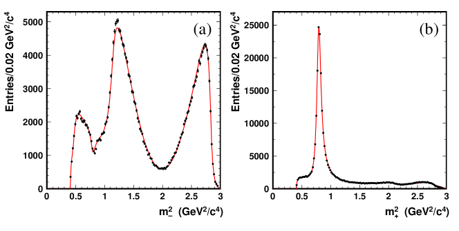
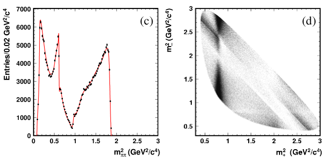
Figure 2: (a) $m_{-}$, (b) $m_{+}$, (c) $m_{\pi\pi}$ and (d) Dalitz plot distribution for $D^{*-}\to\overline{D}{}^{0}\pi_{s}^{-}$, $\overline{D}{}^{0}\to K^{0}_{S}\pi^{+}\pi^{-}$ decays from the $e^{+}e^{-}\to c\bar{c}$ continuum process. The points with error bars show the data; the smooth curve is the fit result.

Table 1: Fit results for $\overline{D}{}^{0}\to K^{0}_{S}\pi^{+}\pi^{-}$ decay. Errors are statistical only.

Intermediate state	Amplitude	Phase (∘)	Fit fraction
$K^{0}_{S}\sigma_{1}$	$1.43\pm 0.07$	$212\pm 3$	9.8%
$K^{0}_{S}\rho^{0}$	$1.0$ (fixed)	0 (fixed)	21.6%
$K^{0}_{S}\omega$	$0.0314\pm 0.0008$	$110.8\pm 1.6$	0.4%
$K^{0}_{S}f_{0}(980)$	$0.365\pm 0.006$	$201.9\pm 1.9$	4.9%
$K^{0}_{S}\sigma_{2}$	$0.23\pm 0.02$	$237\pm 11$	0.6%
$K^{0}_{S}f_{2}(1270)$	$1.32\pm 0.04$	$348\pm 2$	1.5%
$K^{0}_{S}f_{0}(1370)$	$1.44\pm 0.10$	$82\pm 6$	1.1%
$K^{0}_{S}\rho^{0}(1450)$	$0.66\pm 0.07$	$9\pm 8$	0.4%
$K^{*}(892)^{+}\pi^{-}$	$1.644\pm 0.010$	$132.1\pm 0.5$	61.2%
$K^{*}(892)^{-}\pi^{+}$	$0.144\pm 0.004$	$320.3\pm 1.5$	0.55%
$K^{*}(1410)^{+}\pi^{-}$	$0.61\pm 0.06$	$113\pm 4$	0.05%
$K^{*}(1410)^{-}\pi^{+}$	$0.45\pm 0.04$	$254\pm 5$	0.14%
$K_{0}^{*}(1430)^{+}\pi^{-}$	$2.15\pm 0.04$	$353.6\pm 1.2$	7.4%
$K_{0}^{*}(1430)^{-}\pi^{+}$	$0.47\pm 0.04$	$88\pm 4$	0.43%
$K_{2}^{*}(1430)^{+}\pi^{-}$	$0.88\pm 0.03$	$318.7\pm 1.9$	2.2%
$K_{2}^{*}(1430)^{-}\pi^{+}$	$0.25\pm 0.02$	$265\pm 6$	0.09%
$K^{*}(1680)^{+}\pi^{-}$	$1.39\pm 0.27$	$103\pm 12$	0.36%
$K^{*}(1680)^{-}\pi^{+}$	$1.2\pm 0.2$	$118\pm 11$	0.11%
non-resonant	$3.0\pm 0.3$	$164\pm 5$	9.7%

IV Dalitz plot analysis of $B^{+}\to D^{(*)}K^{(*)+}$ decays

In our previous analyses, the two Dalitz distributions corresponding to the decays of $B^{+}$ and $B^{-}$ were fitted simultaneously to give the parameters $r$, $\phi_{3}$ and $\delta$. Confidence intervals were then calculated using a frequentist technique, relying on toy MC simulation. In this approach, there was a bias in the fitted value of the (positive definite) parameter $r$, and the errors on $\phi_{3}$ and $\delta$ were also $r$-dependent.

In the present analysis, we use a method similar to that of BaBar babar_phi3_2 : fitting the Dalitz distributions of the $B^{+}$ and $B^{-}$ samples separately, using Cartesian parameters $x_{\pm}=r_{\pm}\cos(\pm\phi_{3}+\delta)$ and $y_{\pm}=r_{\pm}\sin(\pm\phi_{3}+\delta)$, where the indices “$+$” and “$-$” correspond to $B^{+}$ and $B^{-}$ decays, respectively. Note that in this approach the amplitude ratios ($r_{+}$ and $r_{-}$) are not constrained to be equal for the $B^{+}$ and $B^{-}$ samples. Confidence intervals in $r$, $\phi_{3}$ and $\delta$ are then obtained from the $(x_{\pm},y_{\pm})$ using a frequentist technique. The advantage of this approach is low bias and simple distributions of the fitted parameters, at the price of fitting in a space with higher dimensionality $(x_{+},y_{+},x_{-},y_{-})$ than that of the physical parameters $(r,\phi_{3},\delta)$; see Section IV.5.

The fit to a single Dalitz distribution with free parameters $x$ and $y$ is performed by minimizing the negative unbinned likelihood function

$$-2\log L=-2\left[\sum\limits^{n}_{i=1}\log p(m^{2}_{+,i},m^{2}_{-,i},\Delta E_{i},M_{{\rm bc},i})-\log\int\limits_{D}p(m^{2}_{+},m^{2}_{-},\Delta E,M_{\rm bc}))\;dm^{2}_{+}\;dm^{2}_{-}\;d\Delta E\;dM_{\rm bc}\right],$$ (6)

with the Dalitz distribution density $p$ represented as

$$p(m^{2}_{+},m^{2}_{-},\Delta E,M_{\rm bc})=\varepsilon(m^{2}_{+},m^{2}_{-})|f(m^{2}_{+},m^{2}_{-})+(x+iy)f(m^{2}_{-},m^{2}_{+})|^{2}F_{\rm sig}(\Delta E,M_{\rm bc})+F_{\rm bck}(m^{2}_{+},m^{2}_{-},\Delta E,M_{\rm bc}),$$ (7)

where $F_{\rm sig}$ is the signal distribution as a function of $\Delta E$ and $M_{\rm bc}$ (represented by the product of two Gaussian shapes), $F_{\rm bck}$ is the distribution of the background, and $\varepsilon(m^{2}_{+},m^{2}_{-})$ is the efficiency distribution over the phase space. As in the study of the sample from continuum $D^{*-}\to\overline{D}{}^{0}\pi_{s}^{-}$ decays, the finite momentum resolution is taken into account by convolving the function (7) with a Gaussian resolution function. The efficiency and the momentum resolution were extracted from the signal MC sample, where the neutral $D$ meson decays according to phase space. The determination of the background contribution and efficiency profile is described below.

IV.1 Backgrounds

To take backgrounds into account in the analysis, their Dalitz plot distributions, $\Delta E-M_{\rm bc}$ distributions (which in general may depend on Dalitz plot region) and relative fractions have to be known. The backgrounds are divided into three categories:

• Continuum background

• $B^{+}\to D^{(*)}\pi^{+}$ background (with $\pi/K$ misidentification). This background is relevant only for the $B^{+}\to DK^{+}$ and $B^{+}\to D^{*}K^{+}$ modes.

• Other $b\bar{b}$ backgrounds.

Continuum background (from the process $e^{+}e^{-}\to q\bar{q}$, where $q=u,d,s,c$) gives the largest contribution. It includes both pure combinatorial background, and continuum $D^{0}$ mesons combined with a random kaon. This type of background is studied in data with $\cos\theta_{\rm thr}$ and Fisher discriminant requirements applied to select continuum events. To check that the Dalitz plot shape of the continuum background selected using these requirements corresponds to that of the signal region, we use a MC sample that includes $e^{+}e^{-}\to q\bar{q}$ ($q=u,d,s,c$) decays. The Dalitz plot distribution of the continuum background is parametrized by a third-order polynomial in the variables $m^{2}_{+}$ and $m^{2}_{-}$ (which represents the combinatorial component) and a sum of $D^{0}$ and $\overline{D}{}^{0}$ shapes for real neutral $D$ mesons combined with random kaons.

The $B^{+}\to D^{(*)}\pi^{+}$ process with a pion misidentified as a kaon is suppressed by the requirements on the $K/\pi$ identification variable $\mathcal{R}_{\rm PID}$ and the CM energy difference. The fraction of this background is obtained by fitting the $\Delta E-M_{\rm bc}$ distribution; the corresponding Dalitz plot distribution is that of a $D^{0}$ without the opposite flavor admixture.

Other $B\bar{B}$ backgrounds, of which the dominant fraction comes from the decay of $D^{(*)0}$ from one $B$ meson, with some particles taken from the other $B$ decay, are investigated with $e^{+}e^{-}\to\Upsilon(4S)\to B\bar{B}$ MC events. The Dalitz plot distribution of the $b\bar{b}$ background is parameterized by a second-order polynomial (for the $B^{+}\to DK^{+}$ and $B^{+}\to DK^{*+}$ modes) or by a linear function (for the $B^{+}\to D^{*}K^{+}$ mode) of $m^{2}_{+}$ and $m^{2}_{-}$, plus a “correct-flavor” $D^{0}$ shape ($\overline{D}{}^{0}$ for $B^{+}$ data and $D^{0}$ for $B^{-}$ data).

IV.2 Efficiency

Knowledge of the absolute value of the reconstruction efficiency is not essential for our analysis. However, the relative variations of the efficiency over the $D^{0}$ decay phase space can affect the fit result. The shapes of the efficiency across the phase space are studied for each mode using signal MC samples with a constant $\overline{D}{}^{0}\to K^{0}_{S}\pi^{+}\pi^{-}$ decay amplitude. The efficiency profiles are fitted with third-order polynomial functions of $m_{+}^{2}$ and $m_{-}^{2}$ symmetric under exchange of $\pi^{+}$ and $\pi^{-}$. The efficiency is nearly flat over the phase space, falling by 10–20% at its edges (relative to the efficiency at the center).

IV.3 Control sample fits

To test the consistency of the fitting procedure, the same procedure was applied to the $B^{+}\to\tilde{D}^{(*)}_{+}\pi^{+}$ and $B\to D^{*-}\pi^{+}$ control samples as to the $B^{+}\to\tilde{D}^{(*)}_{+}K^{(*)+}$ signal. For decays to which only one $D$ flavor can contribute, the fit should return values of the amplitude ratio $r$ consistent with zero. In the case of $B^{+}\to\tilde{D}^{(*)}_{+}\pi^{+}$  a small amplitude ratio $r\sim 0.01$ is expected (due to the small ratio of the weak coefficients $|V_{ub}^{\vphantom{*}}V^{*}_{cd}|/|V_{cb}^{\vphantom{*}}V^{*}_{ud}|\sim 0.02$ and the additional color suppression factor as in the case of $B^{+}\to\tilde{D}_{+}K^{+}$). Deviations from these values can appear if the Dalitz plot distribution is not well described by the fit model.

For the control sample fits, we treat $B^{+}$ and $B^{-}$ data separately, to check for the absence of $CP$ violation. The free parameters of the Dalitz plot fit are $x_{\pm}$ and $y_{\pm}$.

Table 2: Results of fits to test samples in parameters $(x,y)$. Errors are statistical only.

Mode	$x_{-}$	$y_{-}$	$x_{+}$	$y_{+}$
$B^{+}\to D\pi^{+}$	$-0.030\pm 0.015$	$-0.014\pm 0.016$	$-0.003\pm 0.014$	$-0.021\pm 0.018$
$B^{+}\to D^{*}\pi^{+}$	$-0.007\pm 0.035$	$-0.078\pm 0.039$	$\phantom{-}0.004\pm 0.032$	$\phantom{-}0.022\pm 0.039$
$B\to D^{*-}\pi^{+}$	$\phantom{-}0.016\pm 0.030$	$\phantom{-}0.014\pm 0.030$	$\phantom{-}0.026\pm 0.026$	$\phantom{-}0.009\pm 0.036$

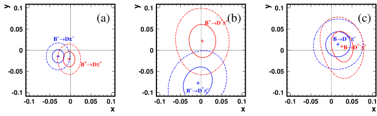
Figure 3: Results of test sample fits with free parameters $x=r\cos\theta$ and $y=r\sin\theta$ for (a) $B^{+}\to D\pi^{+}$, (b) $B^{+}\to D^{*}\pi^{+}$ and (c) $B\to D^{*-}\pi^{+}$ samples, separately for $B^{-}$ and $B^{+}$ data. Contours indicate integer multiples of the standard deviation.

The fit results for the three test samples are presented in Table 2; contour plots showing integer multiples of the standard deviation in the $x_{\pm}$ and $y_{\pm}$ variables for the three test samples are shown in Fig. 3. The results are consistent with $r\sim 0.01$ for the $B^{+}\to D\pi^{+}$ and $B^{+}\to D^{*}\pi^{+}$ modes and with zero for the $B\to D^{*-}\pi^{+}$ mode.

IV.4 Signal fit results

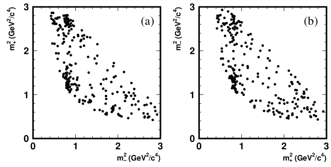
Figure 4: Dalitz plots for the neutral $D$ meson from $B^{-}$ and $B^{+}$ decays, respectively, for the (a,b) $B^{+}\to DK^{+}$, (c,d) $B^{+}\to D^{*}K^{+}$, and (e,f) $B^{+}\to DK^{*+}$ modes. Note that the axes are flipped in the case of $B^{-}$ with respect to $B^{+}$.

Table 3: Results of the signal fits in parameters $(x,y)$. Errors are statistical only.

Mode	$x_{-}$	$y_{-}$	$x_{+}$	$y_{+}$
$B^{+}\to DK^{+}$	$\phantom{-}0.025^{+0.072}_{-0.080}$	$\phantom{-}0.170^{+0.093}_{-0.117}$	$-0.135^{+0.069}_{-0.070}$	$-0.085^{+0.090}_{-0.086}$
$B^{+}\to D^{*}K^{+}$	$-0.128^{+0.167}_{-0.146}$	$-0.339^{+0.172}_{-0.158}$	$\phantom{-}0.032^{+0.120}_{-0.116}$	$\phantom{-}0.008^{+0.137}_{-0.136}$
$B^{+}\to DK^{*+}$	$-0.784^{+0.249}_{-0.295}$	$-0.281^{+0.440}_{-0.335}$	$-0.105^{+0.177}_{-0.167}$	$-0.004^{+0.164}_{-0.156}$

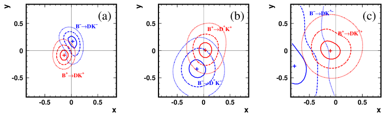
Figure 5: Results of signal fits with free parameters $x=r\cos\theta$ and $y=r\sin\theta$ for (a) $B^{+}\to DK^{+}$, (b) $B^{+}\to D^{*}K^{+}$ and (c) $B^{+}\to DK^{*+}$ samples, separately for $B^{-}$ and $B^{+}$ data. Contours indicate integer multiples of the standard deviation.

The Dalitz distributions of $B^{+}\to\tilde{D}_{+}K^{+}$, $B^{+}\to\tilde{D}^{*}_{+}K^{+}$, and $B^{+}\to\tilde{D}_{+}K^{*+}$ modes for the events in the signal region used in the fits are shown in Fig. 4. The results of the separate $B^{+}$ and $B^{-}$ data fits are shown in Fig. 5. The plots show the constraints on the parameters $x$ and $y$ for the $B^{+}\to\tilde{D}_{+}K^{+}$, $B^{+}\to\tilde{D}^{*}_{+}K^{+}$ and $B^{+}\to\tilde{D}_{+}K^{*+}$ samples. The values of the fit parameters $x_{\pm}$ and $y_{\pm}$ are listed in Table 3.

The fit to the $B^{+}\to DK^{+}$ sample yields $r_{+}$ and $r_{-}$ values close to each other ($r_{+}=0.172$ and $r_{-}=0.160$) with significantly different values of the total phase $\theta_{+}$ and $\theta_{-}$, which is an indication of $CP$ violation. For the $B^{+}\to D^{*}K^{+}$ and $B^{+}\to DK^{*+}$ samples, the values of $r_{+}$ and $r_{-}$ differ (with large errors); in both cases, $r_{+}$ is within a standard deviation of zero, so the corresponding phase $\theta_{+}$ is poorly determined and the significance of $CP$ violation is low.

IV.5 Evaluation of statistical error

We use a frequentist technique to evaluate the statistical significance of the measurements. This method requires knowledge of the probability density function (PDF) of the reconstructed parameters $x$ and $y$ as a function of the true parameters $\bar{x}$ and $\bar{y}$. To obtain this PDF, we employ a “toy” MC technique that uses a simplified MC simulation of the experiment which incorporates the same efficiencies, resolution and backgrounds as used in the fit to the experimental data.

For each mode, 4000 toy MC experiments are made with generated $(\bar{x},\bar{y})$ equal to the experimental fit results. The PDFs obtained are approximately Gaussian, but we observe the width of the distribution to vary with $\bar{x}$ and $\bar{y}$. There is also an offset in the parameters $x,y$ introduced by the fit procedure. The correlations between $x$ and $y$ are negligible. For the $B^{+}\to DK^{+}$ and $B^{+}\to D^{*}K^{+}$ modes, the deviations from the Gaussian shape are small, and taking into account the tails of the distributions has only a minor effect on the fit result. However, the result of the measurement in the $B^{-}\to DK^{*-}$ mode has a relatively large value of $r$ ($r_{-}=0.83\pm 0.28$). For such a large value, the toy MC study shows the existence of significant tails in the observed $x$ and $y$ distributions. To parametrize the shapes of the $x$ and $y$ distributions for the $B^{+}\to DK^{*+}$ sample we perform additional toy MC simulation for different generated $\bar{x}$ and $\bar{y}$, and fit the distributions with the sum of two Gaussians (“narrow” and “wide”). To obtain the PDF shape for any given set of $(\bar{x},\bar{y})$, linear interpolation in $\bar{x}$ and $\bar{y}$ (for the bias of the wide Gaussian relative to the narrow one) and in $\bar{x}^{2}$ and $\bar{y}^{2}$ (for the width and fraction of the wide Gaussian) are used.

To obtain the $(\bar{x},\bar{y})$ dependence of $\sigma_{x}$ and $\sigma_{y}$ and the offset in $x$ and $y$, we generate toy MC experiments at different points in the $(\bar{x},\bar{y})$ plane, corresponding to 4 values of $\theta$ for $r=0.15$ and 8 values of $\theta$ for $r=0.3$ and $r=0.6$. For the $B^{+}\to DK^{*+}$ mode, an additional set of 8 points with $r=0.9$ is added. 200 toy MC experiments are generated at each point. The standard deviation and offset are then parametrized with polynomial functions in $\bar{x}$ and $\bar{y}$.

The offset in $x$ and $y$ is large enough to affect the result of the measurement (up to $0.02$ for the $B^{\pm}\to DK^{\pm}$ mode); it is larger in the $B^{+}\to D^{*}K^{+}$ and $B^{+}\to DK^{*+}$ modes, where the data samples are smaller. To test the effect of sample size, toy MC experiments were generated with event samples ten times larger than those of the $B^{\pm}\to DK^{\pm}$ data: the offset for this sample is less than $5\times 10^{-3}$. This is consistent with the maximum likelihood fit being unbiased in the limit of large sample sizes. For each mode, the offset is included in the PDF for the reconstructed parameters, so the confidence intervals (and central values) for $\phi_{3}$, $r$, $\delta$ are unbiased.

Different implementations of the frequentist technique can be used to obtain the values of the physical parameters. The two most widely used are central (so-called Neyman) intervals, and the unified approach of Feldman and Cousins fc . The latter takes unphysical regions of the parameter space into account. In this analysis, fitting with four parameters $(x_{\pm},y_{\pm})$ in a problem defined by three parameters ($r$, $\phi_{3}$, $\delta$) creates an unphysical region: all $(x_{\pm},y_{\pm})$ values where $r_{+}\neq r_{-}$. For two of the three samples ($B^{+}\to D^{*}K^{+}$ and $B^{+}\to DK^{*+}$) the values of $r_{+}$ and $r_{-}$ differ significantly, i.e. the result for these modes is well into the unphysical region. Central intervals would overestimate the significance of the measurement in this case. Therefore, to obtain the values of the physical parameters $r$, $\phi_{3}$ and $\delta$ (we will refer to this set of parameters as a vector $\mu$) given the measurement result $x_{+}$, $y_{+}$, $x_{-}$ and $y_{-}$ (or vector $z$) we use the Feldman-Cousins approach.

The confidence level $\alpha$ is calculated as

$$\alpha(\mu)=\int\limits_{\mathcal{D}(\mu)}p(z|\mu)dz,$$ (8)

where the integration domain $\mathcal{D}$ is given by likelihood ratio ordering:

$$\frac{p(z|\mu)}{p(z|\mu_{\rm best}(z))}>\frac{p(z_{0}|\mu)}{p(z_{0}|\mu_{\rm best}(z_{0}))}.$$ (9)

Here, $p(z|\mu)$ is the normalized probability density to obtain the measurement result $z$ for a given set of true parameters $\mu$. This PDF is obtained by toy MC simulation. $\mu_{\rm best}(z)$ stands for the best true parameters for a given measurement $z$, i.e. $\mu$ such that $p(z|\mu)$ is maximized for the given $z$. $z_{0}$ is the result of the fit to experimental data.

Table 4: $CP$ fit results. The error intervals are statistical only.

Parameter	$B^{+}\to DK^{+}$ mode		$B^{+}\to D^{*}K^{+}$ mode		$B^{+}\to DK^{*+}$ mode
	$1\sigma$ interval	$2\sigma$ interval	$1\sigma$ interval	$2\sigma$ interval	$1\sigma$ interval	$2\sigma$ interval
$\phi_{3}$	$65.5^{\circ}\;{}^{+19.1^{\circ}}_{-19.9^{\circ}}$	$20.8^{\circ}<\phi_{3}<108.4^{\circ}$	$86.1^{\circ}\;{}^{+37.1^{\circ}}_{-93.1^{\circ}}$	-	$10.8^{\circ}\;{}^{+22.7^{\circ}}_{-57.1^{\circ}}$	-
$r$	$0.165^{+0.056}_{-0.059}$	$0.048<r<0.281$	$0.207^{+0.127}_{-0.131}$	$r<0.510$	$0.549^{+0.231}_{-0.163}$	$0.242<r<1.120$
$\delta$	$147.5^{\circ}\;{}^{+18.7^{\circ}}_{-20.3^{\circ}}$	$100.3^{\circ}<\delta<187.7^{\circ}$	$334.7^{\circ}\;{}^{+36.8^{\circ}}_{-93.6^{\circ}}$	-	$210.2^{\circ}\;{}^{+24.2^{\circ}}_{-57.3^{\circ}}$	-

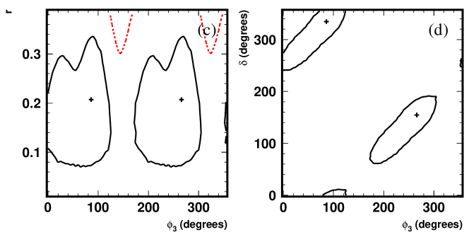
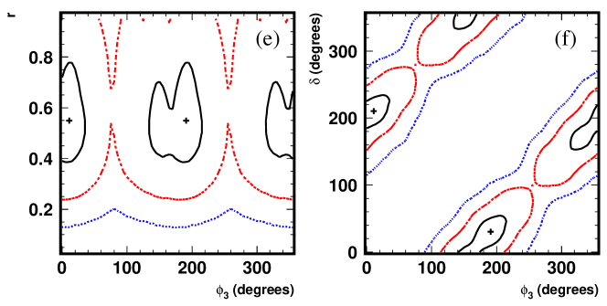
Figure 6: Projections of confidence regions for the (a,b) $B^{+}\to DK^{+}$, (c,d) $B^{+}\to D^{*}K^{+}$, and (e,f) $B^{+}\to DK^{*+}$ modes onto the $(r,\phi_{3})$ and $(\phi_{3},\delta)$ planes. Contours indicate integer multiples of the standard deviation.

Fig 6 shows the projections of the three-dimensional confidence regions onto $(r,\phi_{3})$ and $(\phi_{3},\delta)$ planes. We show the 20%, 74% and 97% confidence level regions, which correspond to one, two, and three standard deviations for a three-dimensional Gaussian distribution. The central values for the parameters $r$, $\phi_{3}$ and $\delta$ with their one and two standard deviation intervals are presented in Table 4. The confidence intervals in Table 4 are calculated from projections of the three-dimensional confidence regions onto each of the parameters. Toy MC studies of the $B^{\pm}\to DK^{\pm}$ mode show that these intervals include the true value of $\phi_{3}$ slightly more often than the confidence levels imply (overcoverage), and are therefore conservative.

IV.6 Estimation of systematic errors

Experimental systematic errors come from uncertainty in the knowledge of the functions used in the signal Dalitz plot fit. These include the Dalitz plot profiles of the backgrounds and the detection efficiency, the momentum resolution description, and, since the background fraction varies depending on the $\Delta E$ and $M_{\rm bc}$ parameters, the parametrizations of the $\Delta E-M_{\rm bc}$ shape of the signal and background.

The systematic errors related to the Dalitz plot shape of the background are studied by using different background descriptions in the signal fit. Instead of the baseline background shape, in which the continuum background is determined from the continuum-enriched experimental sample, and the $b\bar{b}$ background from a MC sample, we perform fits with the background shape represented by only the continuum background parametrization, and the background shape extracted from the $M_{\rm bc}$ sideband ($5.2$ GeV/$c^{2}<M_{\rm bc}<5.26$ GeV/$c^{2}$). The maximum deviation of the parameters $x,y$ from those obtained with the “standard” background parameterization was taken as a measure of the systematic error.

The distribution of the relative detection efficiency over the Dalitz plot is obtained from the MC simulation. To estimate the effect of imperfect simulation of the detector response, we also attempt to obtain the efficiency shape from the experimental data. We expect that the detection efficiency depends primarily on the momentum of the $D$ meson. We also assume that for high momentum $D$ mesons, the efficiency does not vary significantly over phase space and is well determined in the simulation. Therefore, to obtain the relative efficiency distribution for, e.g. the $B^{+}\to DK^{+}$ sample, we use the continuum $D^{*-}\to\overline{D}{}^{0}\pi_{s}^{-}$ sample with $\overline{D}{}^{0}\to K^{0}_{S}\pi^{+}\pi^{-}$ (the one used for the determination of the $\overline{D}{}^{0}\to K^{0}_{S}\pi^{+}\pi^{-}$ amplitude) and compare Dalitz plots for high momentum $\overline{D}{}^{0}$ ($p_{D}>3.5$ GeV/$c$) and $\overline{D}{}^{0}$ in the momentum range corresponding to the $B^{+}\to DK^{+}$ decay ($2.1$ GeV/$c<p_{D}<2.4$ GeV/$c$). If the background is subtracted, the ratio of the event densities for the decays of $\overline{D}{}^{0}$ in different momentum ranges should equal the ratio of detection efficiencies. Once we assume that the efficiency for high momentum $\overline{D}{}^{0}$ is known, the efficiency distribution of $\overline{D}{}^{0}$ from $B^{+}\to DK^{+}$ decay can be calculated. The difference of the parameters $x,y$ between fits using MC-based and data-based efficiency shapes is taken as the corresponding systematic error.

The uncertainty due to momentum resolution is estimated by performing a $\overline{D}{}^{0}$ model fit with a subsequent fit to $B$ decay data without taking the momentum resolution into account. The bias of the $(x,y)$ parameters is negligible, therefore, this systematic uncertainty is neglected.

The uncertainty of the $\Delta E-M_{\rm bc}$ distribution parameterization (which, in particular, leads to uncertainty in the signal-to-background ratio) is taken into account by performing fits using $\Delta E-M_{\rm bc}$ shapes with each of the parameters varied by one standard deviation.

The $\Delta E-M_{\rm bc}$ shape and the total background fraction are extracted from the signal $\Delta E-M_{\rm bc}$ fit. Both continuum and $b\bar{b}$ backgrounds are parametrized by a common $\Delta E-M_{\rm bc}$ density. However, in general, continuum and $b\bar{b}$ (and even each of the sub-components of these backgrounds) may be distributed differently, and the distribution may be correlated with the Dalitz plot distribution. To estimate the contribution of this effect, we make additional fits to data with individual $\Delta E-M_{\rm bc}$ distributions for continuum and $b\bar{b}$ background components extracted from generic MC samples. The corresponding bias is included in the background systematic error.

The results of the study of experimental systematic errors are summarized in Table 5 for each mode. The uncertainties in the parameters $(x,y)$ are then used to obtain the systematic errors for $r$, $\phi_{3}$ and $\delta$ in the combined measurement (see Section IV.8). In our previous analyses belle_phi3_2 ; belle_phi3_3 the systematic error was dominated by a term due to the bias in the fit of $(\phi_{3},r,\delta)$ to the $B^{+}\to D\pi^{+}$ control sample (see Ref. belle_phi3_2 Section V.B). In the present analysis, biases in the fit of $(x_{\pm},y_{\pm})$ to data are small, and are taken into account when forming confidence intervals in $\phi_{3}$, $r$, and $\delta$ (section IV.5). Fitted values for the $B^{+}\to D^{(*)}\pi^{+}$ control samples are consistent with expectations (section IV.3), with statistical precision comparable to the systematic errors listed in Table 5. No additional systematic error is assigned.

Table 5: Systematic errors in $x,y$ variables.

Component	$B^{+}\to DK^{+}$ mode				$B^{+}\to D^{*}K^{+}$ mode				$B^{+}\to DK^{*+}$ mode
	$\Delta x_{-}$	$\Delta y_{-}$	$\Delta x_{+}$	$\Delta y_{+}$	$\Delta x_{-}$	$\Delta y_{-}$	$\Delta x_{+}$	$\Delta y_{+}$	$\Delta x_{-}$	$\Delta y_{-}$	$\Delta x_{+}$	$\Delta y_{+}$
Background shape	0.006	0.015	0.002	0.006	0.011	0.023	0.002	0.004	0.011	0.026	0.002	0.009
Efficiency shape	0.011	0.004	0.017	0.001	0.001	0.001	0.001	0.001	0.024	0.023	0.002	0.009
$\Delta E-M_{\rm bc}$ stat. uncertainty	0.002	0.005	0.002	0.004	0.005	0.009	0.002	0.003	0.006	0.013	0.003	0.003
$\Delta E-M_{\rm bc}$ difference for $q\bar{q}$ and $b\bar{b}$	0.004	0.002	0.000	0.005	0.019	0.012	0.002	0.010	0.010	0.027	0.004	0.001
Total	0.013	0.016	0.017	0.009	0.023	0.027	0.004	0.011	0.029	0.046	0.006	0.013

IV.7 Estimation of model uncertainty

The model used for the $\overline{D}{}^{0}\to K^{0}_{S}\pi^{+}\pi^{-}$ decay amplitude is one of the main sources of systematic error for our analysis. The amplitude is a result of the fit to the experimental Dalitz plot, however since the density of the plot is proportional to the absolute value squared of the decay amplitude, the phase of the complex amplitude is not directly measured. The phase variations across the Dalitz plot are therefore a function of model assumptions and their uncertainties may affect the $\tilde{D}$ Dalitz plot fit.

We use a MC simulation to estimate the effects of the model uncertainties. Event samples are generated according to the Dalitz distribution described by the amplitude given by Eq. 7 with the resonance parameters extracted from our fit to continuum $\overline{D}{}^{0}\to K^{0}_{S}\pi^{+}\pi^{-}$ data, but to fit this distribution different models for $f(m^{2}_{+},m^{2}_{-})$ are used. We scan the phases $\phi_{3}$ and $\delta$ in their physical regions and take the maximum deviations of the fit parameters ($(\Delta r)_{\rm max}$, $(\Delta\phi_{3})_{\rm max}$, and $(\Delta\delta)_{\rm max}$) as model uncertainty estimates. These studies use the value $r=0.15$, close to the one obtained in the dominant $B^{+}\to DK^{+}$ mode.

All the fit models are based on Breit-Wigner parameterizations of resonances as in our default model, but with differences in the treatement of the broad components. By default, we use Blatt-Weisskopf form factors for the $\overline{D}{}^{0}$ meson ($F_{D}$) and intermediate resonances ($F_{r}$) and a $q^{2}$ dependence of the resonance width $\Gamma$ (see cleo_model ): to estimate the effect of the corresponding theoretical uncertainties, we use a fit model without form-factors, and with constant resonant widths $\Gamma_{i}$. We also use a model containing only the largest doubly-Cabibbo-suppressed term $K^{*}(892)^{-}\pi^{+}$, the narrow resonances, $K^{0}_{S}f_{0}(980)$, and $K_{0}^{*}(1430)^{+}\pi^{-}$, with the remainder of the amplitude approximated by the flat non-resonant term.

Other models used are the model with all the resonances from Table 1 excluding the $\sigma_{1}$ or $\sigma_{2}$ states, and the model used by CLEO dkpp_cleo . The results of the study of model uncertainty are summarized in Table 6. The maximum deviation of the parameters is taken as the uncertainty due to the $\overline{D}{}^{0}\to K^{0}_{S}\pi^{+}\pi^{-}$ decay model. Each of the models listed in Table 6 has a reduced $\chi^{2}$ significantly poorer than that of the default model. Therefore, our model uncertainty does not include an additional contribution due to the poor quality of the model fit, discussed in Section III.

Table 6: Estimation of the $\overline{D}{}^{0}\to K^{0}_{S}\pi^{+}\pi^{-}$ decay model uncertainty.

Fit model	$(\Delta r)_{\rm max}$	$(\Delta\phi_{3})_{\rm max}$ (∘)	$(\Delta\delta)_{\rm max}$ (∘)
$F_{r}=F_{D}=1$	0.01	3.1	3.3
$\Gamma(q^{2})={\rm constant}$	0.02	4.7	9.0
$K^{*}(892)^{+}$, $\rho$, $\omega$, $K^{*}(892)^{-}$, $f_{0}(980)$, $K^{*}_{0}(1430)$, non-res.	0.05	8.5	22.9
No $\sigma_{1}$	0.01	2.6	4.3
No $\sigma_{2}$	0.01	0.6	0.7
CLEO model	0.02	5.7	8.7

The mode $B^{+}\to DK^{*+}$ has an additional uncertainty due to the possible presence of a nonresonant $B^{+}\to DK^{0}_{S}\pi^{+}$ component, which can also be treated as a model uncertainty. Since the nonresonant decay is described by the same set of diagrams as $B^{+}\to DK^{*+}$, a similar $CP$ violating effect should be present that in general has values of $r$ and $\delta$ which differ from those for the resonant mode. Thus, for a $\phi_{3}$ measurement without taking the $B^{+}\to DK^{0}_{S}\pi^{+}$ mode into account, its contribution can bias the fit parameters. To estimate the corresponding systematic uncertainty, we first measure the fraction of nonresonant decays within the $B^{+}\to DK^{*+}$ signal region. To increase the sample size for this study, we include additional $\overline{D}{}^{0}$ decay modes: $K^{+}\pi^{-}$, $K^{0}_{S}\pi^{+}\pi^{-}$, $K^{+}\pi^{-}\pi^{0}$ and $K^{+}\pi^{-}\pi^{+}\pi^{-}$. Based on the $B^{+}$ yield in the $K^{*+}$ mass sidebands, and the observed shape of the invariant mass $M_{K^{0}_{S}\pi^{+}}$ of signal candidates, we find an upper limit of 6.3% on the $B^{+}\to DK^{0}_{S}\pi^{+}$ fraction. We then perform a toy MC simulation with a 6.3% nonresonant contribution added to determine the bias of the fit parameters. The fits are performed for various values of the $r$ and $\delta$ parameters of the nonresonant component and various values of the relative phase between $B^{\pm}\to DK^{*\pm}$ and $B^{\pm}\to DK^{0}_{S}\pi^{\pm}$ amplitudes. The maximum bias of the fit parameters is taken as the corresponding systematic error: $\Delta r=0.084$, $\Delta\phi_{3}=8.3^{\circ}$, $\Delta\delta=49.3^{\circ}$. The $\phi_{3}$ bias is significantly smaller than that for the strong phase $\delta$, since $\phi_{3}$ is obtained from a difference of the total phases for $B^{+}$ and $B^{-}$ decays, and a part of the bias cancels in this case.

IV.8 Combined $\phi_{3}$ measurement

The three event samples, $B^{+}\to DK^{+}$, $B^{+}\to D^{*}K^{+}$, and $B^{+}\to DK^{*+}$ are combined in order to improve the sensitivity to $\phi_{3}$. The confidence levels for the combination of three modes are obtained using the same technique as for the single mode. In this case, the vector of physical parameters $\mu=(\phi_{3},r_{DK},\delta_{DK},r_{D*K},\delta_{D*K},r_{DK*},\delta_{DK*})$ and there are twelve measured parameters: four parameters $(x_{\pm},y_{\pm})$ for each of the three modes. The probability density of the measurement result $p(z|\mu)$ is the product of the probability densities for the individual modes.

For each $\mu$, to obtain the confidence level $\alpha(\mu)$, the integral in Eq. 8 is performed over a 12-dimensional space. This requires extensive computation that makes it impractical to scan the whole range of physical parameters to obtain multidimensional confidence regions. However, it is still possible to calculate the confidence intervals for each of the individual parameters.

To calculate the systematic errors for the combined measurement, we vary the measured parameters $x$ and $y$ within their systematic errors. Gaussian distributions are used for the variation, and the systematic biases are assumed to be uncorrelated. For each of the varied parameter sets, the central values of the physical parameters are calculated. The systematic error of the physical parameter is then taken to be equal to the RMS of the resulting distribution.

The error due to the uncertainty in the $\overline{D}{}^{0}\to K^{0}_{S}\pi^{+}\pi^{-}$ amplitude is considered to be equal in all modes. The uncertainty due to the possible contribution of the nonresonant $B^{+}\to DK^{0}_{S}\pi^{+}$ amplitude to $B^{+}\to DK^{*+}$ decay is also included in the model error, by varying the parameters $(x_{\pm},y_{\pm})$ of the $B^{+}\to DK^{*+}$ sample according to the biases $\Delta r$, $\Delta\phi_{3}$, and $\Delta\delta$ obtained above (Section IV.7). We find a contribution of only $1.8^{\circ}$ to the combined $\phi_{3}$ measurement; this is added in quadrature, yielding a total error of $8.7^{\circ}$. For the $r$ and $\delta$ parameters of the $B^{+}\to DK^{*+}$ mode the $B^{+}\to DK^{0}_{S}\pi^{+}$ contribution dominates the model error.

Confidence intervals for the combined measurement together with systematic and model errors are shown in Table 7. The confidence intervals are statistical only and are calculated from projections of the seven-dimensional confidence regions onto each of the parameters. The statistical confidence level of $CP$ violation is 74%. It is defined as the minimum confidence level $\alpha(\mu)$ for the $CP$-conserving set of physical parameters $\mu$ (i.e. the set with $\phi_{3}=0$). The two standard deviation interval (including model and systematic uncertainties) is calculated by adding the doubled systematic and model errors in quadrature to the two standard deviation statistical errors: we find $8^{\circ}<\phi_{3}<111^{\circ}$.

We note that the two standard deviation interval of $\phi_{3}$ is more than twice as wide as the one standard deviation interval. The non-Gaussian errors in $\phi_{3}$ are related to the low significance of $r$; this effect should be reduced with larger data samples in the future. There is also a contribution from the disagreement between the $B^{+}\to DK^{+}$ and $B^{+}\to DK^{*+}$ results, which leads to a second minimum in $\alpha(\mu)$ between the one and two standard deviation levels.

Table 7: Results of the combination of $B^{+}\to DK^{+}$, $B^{+}\to D^{*}K^{+}$, and $B^{+}\to DK^{*+}$ modes.

Parameter	$1\sigma$ statistical interval	$2\sigma$ statistical interval	Systematic error	Model uncertainty
$\phi_{3}$	$53.3^{\circ}\;{}^{+14.8^{\circ}}_{-17.7^{\circ}}$	$11.7^{\circ}<\phi_{3}<107.7^{\circ}$	$2.5^{\circ}$	$8.7^{\circ}$
$r_{DK}$	$0.159^{+0.054}_{-0.050}$	$0.048<r_{DK}<0.271$	0.012	0.049
$\delta_{DK}$	$145.7^{\circ}\;{}^{+19.0^{\circ}}_{-19.7^{\circ}}$	$100.6^{\circ}<\delta_{DK}<185.9^{\circ}$	$3.0^{\circ}$	$22.9^{\circ}$
$r_{D^{*}K}$	$0.175^{+0.108}_{-0.099}$	$0<r_{D^{*}K}<0.407$	0.013	0.049
$\delta_{D^{*}K}$	$302.0^{\circ}\;{}^{+33.8^{\circ}}_{-35.1^{\circ}}$	-	$6.1^{\circ}$	$22.9^{\circ}$
$r_{DK^{*}}$	$0.564^{+0.216}_{-0.155}$	$0.231<r_{DK^{*}}<1.106$	0.041	0.084
$\delta_{DK^{*}}$	$242.6^{\circ}\;{}^{+20.2^{\circ}}_{-23.2^{\circ}}$	$186.0^{\circ}<\delta_{DK^{*}}<300.2^{\circ}$	$2.5^{\circ}$	$49.3^{\circ}$

V Conclusion

We report the results of a measurement of the unitarity triangle angle $\phi_{3}$, using a method based on Dalitz plot analysis of $\overline{D}{}^{0}\to K^{0}_{S}\pi^{+}\pi^{-}$ decay in the process $B^{+}\to D^{(*)}K^{(*)+}$. The measurement of $\phi_{3}$ using this technique was performed based on a 357 fb^-1 data sample collected by the Belle detector. From the combination of $B^{+}\to DK^{+}$, $B^{+}\to D^{*}K^{+}$ and $B^{+}\to DK^{*+}$ modes, we obtain the value $\phi_{3}=53^{\circ}\;{}^{+15^{\circ}}_{-18^{\circ}}\pm 3^{\circ}\pm 9^{\circ}$; of the two possible solutions we choose the one with $0<\phi_{3}<180^{\circ}$. The first error is statistical, the second is experimental systematics and the third is model uncertainty. The two standard deviation interval (including model and systematic uncertainties) is $8^{\circ}<\phi_{3}<111^{\circ}$. The statistical significance of $CP$ violation for the combined measurement is 74%. The method allows us to obtain a value of the ratio of the two interfering $D$ decay amplitudes $r$, which can be used in other $\phi_{3}$ measurements. We obtain $r=0.159^{+0.054}_{-0.050}\pm 0.012\pm 0.049$ for the $B^{+}\to DK^{+}$ mode, $r=0.175^{+0.108}_{-0.099}\pm 0.013\pm 0.049$ for the $B^{+}\to D^{*}K^{+}$ mode and $r=0.564^{+0.216}_{-0.155}\pm 0.041\pm 0.084$ for the $B^{+}\to DK^{*+}$ mode.

Appendix A Model uncertainty in $\bf(x,y)$ parameters

Averaging the $\phi_{3}$ measurements between different methods and different experiments is most conveniently done using the $(x,y)$ parameters, which are better-behaved than $(r,\phi_{3},\delta)$. This requires errors (including model uncertainty) to be expressed in terms of the $(x,y)$ parameters, but our model uncertainty study was performed in $(r,\phi_{3},\delta)$. To calculate the errors due to the $\overline{D}{}^{0}\to K^{0}_{S}\pi^{+}\pi^{-}$ decay model uncertainty in $(x,y)$ we propagate the $(r,\phi_{3},\delta)$ errors under the assumption that there is no correlation between them. This approach results in substantial off-diagonal terms. The correlation matrix for the vector $z=(x_{DK^{-}},y_{DK^{-}},x_{DK^{+}},y_{DK^{+}},x_{D^{*}K^{-}},y_{D^{*}K^{-}},x_{D^{*}K^{+}},y_{D^{*}K^{+}},x_{DK^{*-}},y_{DK^{*-}},x_{DK^{*+}},y_{DK^{*+}})$ is defined as

$$(\mathcal{C}_{D^{0}})_{ij}=\overline{\Delta z_{i}\Delta z_{j}},$$

and is equal to

$$\mathcal{C}_{D^{0}}=\left(\begin{array}[]{rrrrrrrrrrrr}459&10&-104&332&-56&21&6&62&-12&68&64&30\\ 10&241&-232&-64&-3&1&0&2&0&3&3&2\\ -104&-232&264&-68&-18&7&2&20&-3&22&20&10\\ 332&-64&-68&436&55&-22&-4&-57&9&-66&-59&-30\\ -56&-3&-18&55&515&-108&-54&400&10&-70&-64&-33\\ 21&1&7&-22&-108&282&-235&-135&-4&27&25&13\\ 6&0&2&-4&-54&-235&242&26&-1&7&5&2\\ 62&2&20&-57&400&-135&26&556&-13&76&69&33\\ -12&0&-3&9&10&-4&-1&-13&939&36&-328&878\\ 68&3&22&-66&-70&27&7&76&36&732&-556&-99\\ 64&3&20&-59&-64&25&5&69&-328&-556&769&-86\\ 30&2&10&-30&-33&13&2&33&878&-99&-86&904\\ \end{array}\right)\times 10^{-5}.$$ (10)

The uncertainty due to the non-resonant contribution to the $B^{+}\to DK^{*+}$ mode produces an additional contribution

$$\mathcal{C}_{DK\pi}=\left(\begin{array}[]{rrrr}766&-371&113&828\\ -371&2984&-2605&-1136\\ 113&-2605&2601&919\\ 828&-1136&919&1150\\ \end{array}\right)\times 10^{-5}.$$ (11)

to the terms in $(x_{DK^{*-}},y_{DK^{*-}},x_{DK^{*+}},y_{DK^{*+}})$.

References

(1)
M. Kobayashi and T. Maskawa, Prog. Theor. Phys. 49, 652 (1973);
N. Cabibbo, Phys. Rev. Lett. 10, 531 (1963).
(2)
I. I. Bigi and A. I. Sanda, Phys. Lett. B211, 213 (1988);
A. B. Carter and A. I. Sanda, Phys. Rev. Lett 45, 952 (1980).
(3)
M. Gronau and D. London, Phys. Lett. B253, 483 (1991);
M. Gronau and D. Wyler, Phys. Lett. B265, 172 (1991).
(4)
I. Dunietz, Phys. Lett. B270, 75 (1991).
(5)
D. Atwood, G. Eilam, M. Gronau and A. Soni, Phys. Lett. B341, 372 (1995).
(6)
D. Atwood, I. Dunietz and A. Soni, Phys. Rev. Lett. 78, 3257 (1997);
D. Atwood, I. Dunietz and A. Soni, Phys. Rev. D 63, 036005 (2001).
(7)
A. Giri, Yu. Grossman, A. Soffer, J. Zupan, Phys. Rev. D 68,
054018 (2003).
(8)
A. Bondar. Proceedings of BINP Special Analysis Meeting on Dalitz Analysis,
24-26 Sep. 2002, unpublished.
(9)
M. Gronau, Phys. Lett. B557, 198 (2003).
(10)
Belle Collaboration, A. Poluektov et al., Phys. Rev. D 70, 072003 (2004).
(11)
Belle Collaboration, K. Abe et al., hep-ex/0411049.
(12)
BABAR Collaboration, B. Aubert et al., Phys. Rev. Lett. 95, 121802 (2005).
(13)
BABAR Collaboration, B. Aubert et al., hep-ex/0507101.
(14)
Belle Collaboration, K. Abe et al., hep-ex/0504013.
(15)
Belle Collaboration, A. Abashian et al., Nucl. Instr. and Meth. A 479, 117 (2002).
(16)
Y. Ushiroda (Belle SVD2 Group), Nucl. Instr. and Meth. A 511, 6 (2003).
(17)
CLEO Collaboration, D. M. Asner et al., Phys. Rev. D 53, 1039
(1996).
(18)
ARGUS Collaboration, H. Albrecht et al., Phys. Lett. B 241, 278
(1990).
(19)
CLEO Collaboration, H. Muramatsu et al., Phys. Rev. Lett.
89, 251802 (2002), Erratum-ibid: 90, 059901 (2003).
(20)
CLEO Collaboration, S. Kopp et al., Phys. Rev. D 63, 092001 (2001).