Measurement of Branching Fractions and $C\!P$-Violating Charge Asymmetries for $B$ Meson Decays to $D^{(*)}\kern 2.87996pt\overline{\kern-2.87996ptD}{}^{(*)}$, and Implications for the CKM Angle $\gamma$

Abstract

We present measurements of the branching fractions and charge asymmetries of $B$ decays to all $D^{(*)}\kern 1.99997pt\overline{\kern-1.99997ptD}{}^{(*)}$ modes. Using 232 million $B\kern 1.79993pt\overline{\kern-1.79993ptB}{}$ pairs recorded on the $\mathchar 28935\relax(4S)$ resonance by the BABAR detector at the $e^{+}e^{-}$ asymmetric $B$ factory PEP-II at the Stanford Linear Accelerator Center, we measure the branching fractions

$$\mathcal{B}(B^{0}\rightarrow D^{*+}D^{*-}) = (8.1\pm 0.6\pm 1.0)\times 10^{-4},$$

$$\mathcal{B}(B^{0}\rightarrow D^{*\pm}D^{\mp}) = (5.7\pm 0.7\pm 0.7)\times 10^{-4},$$

$$\mathcal{B}(B^{0}\rightarrow D^{+}D^{-}) = (2.8\pm 0.4\pm 0.5)\times 10^{-4},$$

$$\mathcal{B}(B^{+}\rightarrow D^{*+}\kern 1.99997pt\overline{\kern-1.99997ptD}{}^{*0}) = (8.1\pm 1.2\pm 1.2)\times 10^{-4},$$

$$\mathcal{B}(B^{+}\rightarrow D^{*+}\kern 1.99997pt\overline{\kern-1.99997ptD}{}^{0}) = (3.6\pm 0.5\pm 0.4)\times 10^{-4},$$

$$\mathcal{B}(B^{+}\rightarrow D^{+}\kern 1.99997pt\overline{\kern-1.99997ptD}{}^{*0}) = (6.3\pm 1.4\pm 1.0)\times 10^{-4},$$

$$\mbox{and}\;\mathcal{B}(B^{+}\rightarrow D^{+}\kern 1.99997pt\overline{\kern-1.99997ptD}{}^{0}) = (3.8\pm 0.6\pm 0.5)\times 10^{-4},$$

where in each case the first uncertainty is statistical and the second systematic. We also determine the limits

$$\mathcal{B}(B^{0}\rightarrow D^{*0}\kern 1.99997pt\overline{\kern-1.99997ptD}{}^{*0}) < 0.9\times 10^{-4},$$

$$\mathcal{B}(B^{0}\rightarrow D^{*0}\kern 1.99997pt\overline{\kern-1.99997ptD}{}^{0}) < 2.9\times 10^{-4},$$

$$\mbox{and}\;\mathcal{B}(B^{0}\rightarrow D^{0}\kern 1.99997pt\overline{\kern-1.99997ptD}{}^{0}) < 0.6\times 10^{-4},$$

each at 90% confidence level. All decays above denote either member of a charge conjugate pair. We also determine the $C\!P$-violating charge asymmetries

$$\mathcal{A}(B^{0}\rightarrow D^{*\pm}D^{\mp}) = 0.03\pm 0.10\pm 0.02,$$

$$\mathcal{A}(B^{+}\rightarrow D^{*+}\kern 1.99997pt\overline{\kern-1.99997ptD}{}^{*0}) = -0.15\pm 0.11\pm 0.02,$$

$$\mathcal{A}(B^{+}\rightarrow D^{*+}\kern 1.99997pt\overline{\kern-1.99997ptD}{}^{0}) = -0.06\pm 0.13\pm 0.02,$$

$$\mathcal{A}(B^{+}\rightarrow D^{+}\kern 1.99997pt\overline{\kern-1.99997ptD}{}^{*0}) = 0.13\pm 0.18\pm 0.04,$$

$$\mbox{and}\;\mathcal{A}(B^{+}\rightarrow D^{+}\kern 1.99997pt\overline{\kern-1.99997ptD}{}^{0}) = -0.13\pm 0.14\pm 0.02.$$

Additionally, when we combine these results with information from time-dependent $C\!P$ asymmetries in $B^{0}\rightarrow D^{(*)+}D^{(*)-}$ decays and world-averaged branching fractions of $B$ decays to $D_{s}^{(*)}\kern 1.99997pt\overline{\kern-1.99997ptD}{}^{(*)}$ modes, we find the CKM phase $\gamma$ is favored to lie in the range $[0.07-2.77]$ radians (with a +0 or $+\pi$ radians ambiguity) at 68% confidence level.

I Introduction

We report on measurements of branching fractions of neutral and charged $B$-meson decays to the ten double-charm final states $D^{(*)}\kern 1.99997pt\overline{\kern-1.99997ptD}{}^{(*)}$. For the four charged $B$ decays to $D^{(*)}\kern 1.99997pt\overline{\kern-1.99997ptD}{}^{(*)}$ and for neutral $B$ decays to $D^{*\pm}D^{\mp}$, we also measure the direct $C\!P$-violating time-integrated charge asymmetry

$$\mathcal{A}_{C\!P}\equiv\frac{\Gamma^{-}-\Gamma^{+}}{\Gamma^{-}+\Gamma^{+}},$$ (1)

where in the case of the charged $B$ decays, the superscript on $\Gamma$ corresponds to the sign of the $B^{\pm}$ meson, and for $D^{*\pm}D^{\mp}$, $\Gamma^{+}$ refers to $D^{*-}D^{+}$ and $\Gamma^{-}$ to $D^{*+}D^{-}$.

In the neutral $B\rightarrow D^{(*)+}D^{(*)-}$ decays, the interference of the dominant tree diagram (see Fig. 1a) with the neutral $B$ mixing diagram is sensitive to the Cabibbo-Kobayashi-Maskawa (CKM) phase $\beta\equiv\arg\left[\,-V_{\rm cd}V_{\rm cb}^{*}/V_{\rm td}V_{\rm tb}^{*}\,\right]$, where $V$ is the CKM quark mixing matrix CKM . However, the theoretically uncertain contributions of penguin diagrams (Fig. 1b) with different weak phases are potentially significant and may shift both the observed $C\!P$ asymmetries and the branching fractions by amounts that depend on the ratios of the penguin to tree contributions and their relative phases. A number of theoretical estimates exist for the resulting values of the branching fractions and $C\!P$ asymmetries gronauetc ; rosner ; sandaxing ; phamxing ; xing2 .

The penguin-tree interference in neutral and charged $B\rightarrow D^{(*)}\kern 1.99997pt\overline{\kern-1.99997ptD}{}^{(*)}$ decays can provide sensitivity to the angle $\gamma=\arg\left[\,-V_{\rm ud}V_{\rm ub}^{*}/V_{\rm cd}V_{\rm cb}^{*}\,\right]$ DL ; ADL . With additional information on the branching fractions of $B\rightarrow D^{(*)}_{s}\kern 1.99997pt\overline{\kern-1.99997ptD}{}^{(*)}$ decays, the weak phase may be extracted, assuming SU(3) flavor symmetry between $B\rightarrow D^{(*)}\kern 1.99997pt\overline{\kern-1.99997ptD}{}^{(*)}$ and $B\rightarrow D^{(*)}_{s}\kern 1.99997pt\overline{\kern-1.99997ptD}{}^{(*)}$. For this analysis, we assume that the breaking of SU(3) can be parametrized via the ratios of decay constants $f_{D_{s}^{(*)}}/f_{D^{(*)}}$, which are quantities that can be determined either with lattice QCD or from experimental measurements lattice .

Figure 1: Feynman graphs for $B\rightarrow D^{(*)}\kern 1.99997pt\overline{\kern-1.99997ptD}{}^{(*)}$ decays: the tree (a) and penguin (b) diagrams are the leading terms for both $B^{0}$ $\rightarrow D^{(*)+}D^{(*)-}$ and $B^{+}$ $\rightarrow D^{(*)+}\kern 1.99997pt\overline{\kern-1.99997ptD}{}^{(*)0}$ decays, whereas the exchange (c) and annihilation (d) diagrams (the latter of which is OZI-suppressed) are the lowest-order terms for $B^{0}$ $\rightarrow D^{(*)0}\kern 1.99997pt\overline{\kern-1.99997ptD}{}^{(*)0}$ decays.

In addition to presenting measurements of the $B^{0}$ $\rightarrow D^{(*)+}D^{(*)-}$ and $B^{+}$ $\rightarrow D^{(*)+}\kern 1.99997pt\overline{\kern-1.99997ptD}{}^{(*)0}$ branching fractions, and the $C\!P$-violating charge asymmetries for the latter modes and for $B^{0}$ $\rightarrow D^{*\pm}D^{\mp}$, we search for the color-suppressed decay modes $B^{0}$ $\rightarrow D^{(*)0}\kern 1.99997pt\overline{\kern-1.99997ptD}{}^{(*)0}$, which have not been previously measured, and determine limits on those branching fractions CC . If observed, the decays $B^{0}$ $\rightarrow D^{(*)0}\kern 1.99997pt\overline{\kern-1.99997ptD}{}^{(*)0}$ would provide evidence of $W$-exchange or annihilation contributions (see Fig. 1c,1d). In principle, these decays could also provide sensitivity to the CKM phase $\beta$ if sufficient data were available. By combining all of these results with information from time-dependent $C\!P$ asymmetries in $B^{0}\rightarrow D^{(*)+}D^{(*)-}$ decays and world-averaged branching fractions of $B$ decays to $D_{s}^{(*)}\kern 1.99997pt\overline{\kern-1.99997ptD}{}^{(*)}$ modes, we determine the implications for $\gamma$ using the method of Refs. DL ; ADL .

II Detector and Data

The results presented in this paper are based on data collected with the BABAR detector BABARNIM at the PEP-II asymmetric-energy $e^{+}e^{-}$ collider pep located at the Stanford Linear Accelerator Center. The integrated luminosity is 210.5 $\mbox{\,fb}^{-1}$, corresponding to 231.7 million $B\kern 1.79993pt\overline{\kern-1.79993ptB}{}$ pairs, recorded at the $\mathchar 28935\relax(4S)$ resonance (“on-peak”, at a center-of-mass (c.m.) energy $\sqrt{s}=10.58\ \mathrm{\,Ge\kern-1.00006ptV}$).

The asymmetric beam configuration in the laboratory frame provides a boost of $\beta\gamma=0.56$ to the $\mathchar 28935\relax(4S)$. Charged particles are detected and their momenta measured by the combination of a silicon vertex tracker (SVT), consisting of five layers of double-sided detectors, and a 40-layer central drift chamber (DCH), both operating in the 1.5-T magnetic field of a solenoid. For tracks with transverse momentum greater than 120 ${\mathrm{\,Me\kern-1.00006ptV\!/}c}$, the DCH provides the primary charged track finding capability. The SVT provides complementary standalone track finding for tracks of lower momentum, allowing for reconstruction of charged tracks with transverse momentum $p_{T}$ as low as 60 ${\mathrm{\,Me\kern-1.00006ptV\!/}c}$, with efficiencies in excess of 85%. This ability to reconstruct tracks with low $p_{T}$ efficiently is necessary for reconstruction of the slow charged pions from $D^{*+}$ $\rightarrow D^{0}\pi^{+}$ decays in $B\rightarrow D^{(*)}\kern 1.99997pt\overline{\kern-1.99997ptD}{}^{(*)}$ signal events. The transverse momentum resolution for the combined tracking system is $\sigma_{p_{T}}/p_{T}=0.0013p_{T}+0.0045$, where $p_{T}$ is measured in ${\mathrm{\,Ge\kern-1.00006ptV\!/}c}$. Photons are detected and their energies measured by a CsI(Tl) electromagnetic calorimeter (EMC). The photon energy resolution is $\sigma_{E}/E=\left\{2.3/E(\mathrm{\,Ge\kern-1.00006ptV})^{1/4}\oplus 1.4\right\}\%$, and their angular resolution with respect to the interaction point is $\sigma_{\theta}=\mbox{(4.2 mrad)}/\sqrt{E(\mathrm{\,Ge\kern-1.00006ptV})}$. The measured $\pi^{0}$ mass resolution for $\pi^{0}$’s with laboratory momentum in excess of 1 ${\mathrm{\,Ge\kern-1.00006ptV\!/}c}$ is approximately 6 ${\mathrm{\,Me\kern-1.00006ptV\!/}c^{2}}$.

Charged-particle identification (PID) is provided by an internally reflecting ring-imaging Cherenkov light detector (DIRC) covering the central region, and the most probable energy loss ($\mathrm{d}E/\mathrm{d}x$) in the tracking devices. The Cherenkov angle resolution of the DIRC is measured to be 2.4 mrad, which provides over $5\sigma$ separation between charged kaons and pions at momenta of less than $2~{}{\mathrm{\,Ge\kern-1.00006ptV\!/}c}$. The $\mathrm{d}E/\mathrm{d}x$ resolution from the drift chamber is typically about $7.5\%$ for pions. Additional information to identify and reject electrons and muons is provided by the EMC and detectors embedded between the steel plates of the magnetic flux return (IFR).

III Candidate Reconstruction and $B$ Meson Selection

Given the high multiplicity of the final states studied, very high combinatorial background levels are expected. Selection criteria (described in Sec. III A–E) are designed to minimize the expected statistical error on the $B$ branching fractions (as described in Sec. III F). A GEANT4-based GEANT4 Monte Carlo (MC) simulation of the material composition and the instrumentation response of the BABAR detector is used to optimize signal selection criteria and evaluate signal detection efficiency. We retain sufficient sidebands in the discriminating variables to characterize the background in subsequent fits.

III.1 Charged track and $K^{0}_{\scriptscriptstyle S}$ selection

Charged particle tracks are selected via pattern recognition algorithms using measurements from the SVT and DCH detectors. We additionally require all charged-particle tracks (except for those from $K^{0}_{\scriptscriptstyle S}\rightarrow\pi^{+}\pi^{-}$ decays) to originate within 10 cm along the beam axis and 1.5 cm in the plane perpendicular to the beam axis of the center of the beam crossing region. To ensure a well-measured momentum, all charged-particle tracks except those from $K^{0}_{\scriptscriptstyle S}\rightarrow\pi^{+}\pi^{-}$ decays and $\pi^{+}$ from $D^{*+}\rightarrow D^{0}\pi^{+}$ decays must also be reconstructed from at least 12 measurements in the DCH. All tracks that meet these criteria are considered as charged pion candidates.

Tracks may be identified as kaons based on a likelihood selection developed from Cherenkov angle and $\mathrm{d}E/\mathrm{d}x$ information from the DIRC and tracking detectors respectively. For the typical laboratory momentum spectrum of the signal kaons, this selection has an efficiency of about 85% and a purity of greater than 98%, as determined from control samples of $D^{*+}\rightarrow D^{0}\pi^{+}$, $D^{0}\rightarrow K^{-}\pi^{+}$ decays.

We require $K^{0}_{\scriptscriptstyle S}\rightarrow\pi^{+}\pi^{-}$ candidates to have an invariant mass within 15 ${\mathrm{\,Me\kern-1.00006ptV\!/}c^{2}}$ of the nominal $K^{0}_{\scriptscriptstyle S}$ mass PDG2004 . The probability that the two daughter tracks originate from the same point in space must be greater than 0.1%. The transverse flight distance of the $K^{0}_{\scriptscriptstyle S}$ from the primary event vertex must be both greater than $3\sigma$ from zero (where $\sigma$ is the measured uncertainty on the transverse flight length) and also greater than 2 mm.

III.2 Photon and $\pi^{0}$ selection

Photons are reconstructed from energy deposits in the electromagnetic calorimeter which are not associated with a charged track. To reject backgrounds from electronics noise, machine background, and hadronic interactions in the EMC, we require that all photon candidates have an energy greater than 30 $\mathrm{\,Me\kern-1.00006ptV}$ in the laboratory frame and to have a lateral shower shape consistent with that of a photon. Neutral pions are reconstructed from pairs of photon candidates whose energies in the laboratory frame sum to more than 200 $\mathrm{\,Me\kern-1.00006ptV}$. The $\pi^{0}$ candidates must have an invariant mass between 115 and 150 ${\mathrm{\,Me\kern-1.00006ptV\!/}c^{2}}$. The $\pi^{0}$ candidates that meet these criteria, when combined with other tracks or neutrals to form $B$ candidates, are then constrained to originate from their expected decay points, and their masses are constrained to the nominal value PDG2004 . This procedure improves the mass and energy resolution of the parent particles.

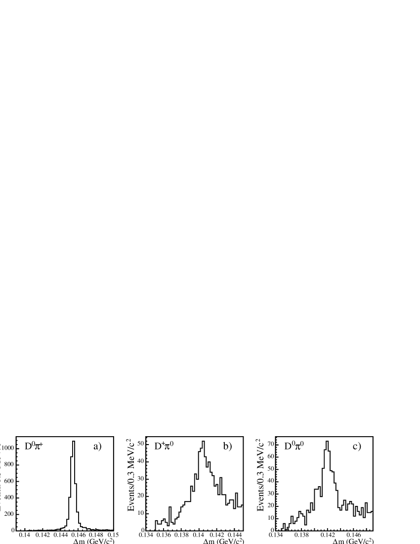
Figure 2: Distributions of $\Delta m$ in the full data sample for three $D^{*}$ decay modes. Plot a) shows $\Delta m(D^{*+}-D^{0})$ for $D^{*+}\rightarrow D^{0}\pi^{+}$ decays where $D^{0}$ decays to $K^{-}\pi^{+}$. Plot b) shows $\Delta m(D^{*+}-D^{+})$ for $D^{*+}\rightarrow D^{+}\pi^{0}$ decays where $D^{+}$ decays to $K^{-}\pi^{+}\pi^{+}$. Plot c) shows $\Delta m(D^{*0}-D^{0})$ for $D^{*0}\rightarrow D^{0}\pi^{0}$ decays where $D^{0}$ decays to $K^{-}\pi^{+}$. Nominal values for $\Delta m$ are 145.4 ${\mathrm{\,Me\kern-1.00006ptV\!/}c^{2}}$, 140.6 ${\mathrm{\,Me\kern-1.00006ptV\!/}c^{2}}$, and 142.1 ${\mathrm{\,Me\kern-1.00006ptV\!/}c^{2}}$ for the three cases respectively PDG2004 .

III.3 Event selection

We select $B\kern 1.79993pt\overline{\kern-1.79993ptB}{}$ events by applying criteria on the track multiplicity and event topology. At least three reconstructed tracks, each with transverse momentum greater than 100 ${\mathrm{\,Me\kern-1.00006ptV\!/}c}$, are required in the laboratory polar angle region $0.41<\theta_{\rm lab}<2.54$. The event must have a total measured energy in the laboratory frame greater than 4.5 $\mathrm{\,Ge\kern-1.00006ptV}$ to reject beam-related background. The ratio of Fox-Wolfram moments $H_{2}/H_{0}$ FoxW is a parameter between 0 (for “perfectly spherical” events) and 1 (for “perfectly jet-like” events), and we require this ratio to be less than 0.6 for each event, in order to help reject non-$B\kern 1.79993pt\overline{\kern-1.79993ptB}{}$ background. This criterion rejects between 30 and 50 percent of non-$B\kern 1.79993pt\overline{\kern-1.79993ptB}{}$ background (depending on the decay mode), while keeping almost all of the signal decays.

III.4 $D$ and $D^{*}$ meson selection

We reconstruct $D^{0}$ mesons in the four decay modes $D^{0}\rightarrow K^{-}\pi^{+}$, $D^{0}\rightarrow K^{-}\pi^{+}\pi^{0}$, $D^{0}\rightarrow K^{-}\pi^{+}\pi^{-}\pi^{+}$, and $D^{0}\rightarrow K^{0}_{\scriptscriptstyle S}\pi^{+}\pi^{-}$, and $D^{+}$ mesons in the two decay modes $D^{+}\rightarrow K^{-}\pi^{+}\pi^{+}$ and $D^{+}\rightarrow K^{0}_{\scriptscriptstyle S}\pi^{+}$. We require $D^{0}$ and $D^{+}$ candidates to have reconstructed masses within $\pm 20$ ${\mathrm{\,Me\kern-1.00006ptV\!/}c^{2}}$ of their nominal masses PDG2004 , except for $D^{0}\rightarrow K^{-}\pi^{+}\pi^{0}$, for which we require $\pm 40$ ${\mathrm{\,Me\kern-1.00006ptV\!/}c^{2}}$ due to the poorer resolution for modes containing $\pi^{0}$’s. These criteria correspond to approximately $2.5\sigma$ of the respective mass resolutions. The $D^{0}\rightarrow K^{-}\pi^{+}\pi^{0}$ decays must also satisfy a criterion on the reconstructed invariant masses of the $K^{-}\pi^{+}$ and $K^{-}\pi^{0}$ pairs: the combination of reconstructed invariant masses must lie at a point in the $K^{-}\pi^{+}\pi^{0}$ Dalitz plot Dalitz for which the expected density normalized to the maximum density (“Dalitz weight”) is at least 6%. Additionally, the daughters of $D^{0}$ and $D^{+}$ candidates must have a probability of originating from a common point in space greater than 0.1%, and are then constrained both to originate from that common spatial point and to have their respective nominal invariant masses.

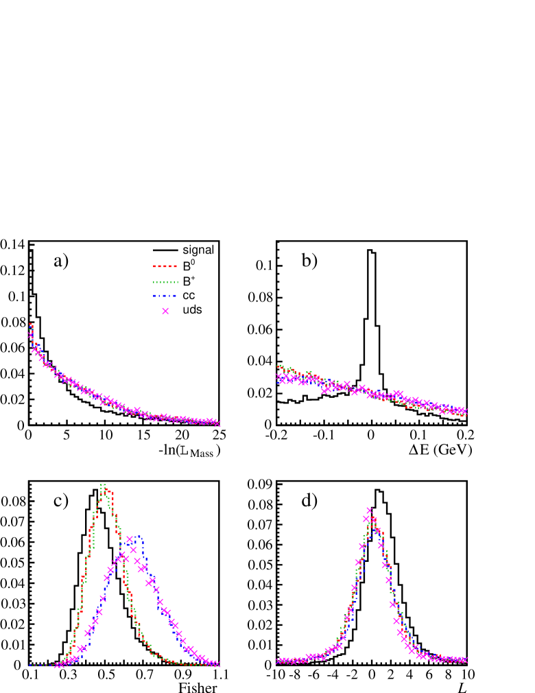
Figure 3: Distributions of signal selection variables: a) the likelihood variable $-\ln({\cal L}_{\rm Mass})$, b) the $\Delta E$ variable, c) the Fisher discriminant $\mathcal{F}$, and d) the $D$-meson flight length variable $L$, each for the representative signal mode $B^{0}$ $\rightarrow D^{0}\kern 1.99997pt\overline{\kern-1.99997ptD}{}^{0}$, and for the corresponding combinatorial background from $B^{0}{\kern-1.60004pt\kern 1.79993pt\overline{\kern-1.79993ptB}{}^{0}}$, $B^{+}{\kern-1.60004ptB^{-}}$, $c\overline{c}$, and ($u\overline{u}$ +$d\overline{d}$ +$s\overline{s}$) MC simulated decays respectively. In each plot, the component distributions are normalized to have the same area below the curves.

Candidate $D^{*+}$ and $D^{*0}$ mesons are reconstructed in the decay modes $D^{*+}\rightarrow D^{0}\pi^{+}$, $D^{*+}\rightarrow D^{+}\pi^{0}$, $D^{*0}\rightarrow D^{0}\pi^{0}$, and $D^{*0}\rightarrow D^{0}\gamma$, using pairs of selected $D^{0}$, $D^{+}$, $\pi^{0}$, $\pi^{+}$, and $\gamma$ candidates. The $\pi^{+}$ from $D^{*+}\rightarrow D^{0}\pi^{+}$ decays is additionally required to have a c.m. momentum of less than 450 ${\mathrm{\,Me\kern-1.00006ptV\!/}c}$. Candidate $\pi^{0}$ mesons from $D^{*+}\rightarrow D^{+}\pi^{0}$ and $D^{*0}\rightarrow D^{0}\pi^{0}$ are required to have c.m. momenta $p^{*}$ in the range $70<p^{*}<450$ ${\mathrm{\,Me\kern-1.00006ptV\!/}c}$. Photons from $D^{*0}\rightarrow D^{0}\gamma$ decays are required to have energies in the laboratory frame greater than 100 $\mathrm{\,Me\kern-1.00006ptV}$ and c.m. energies less than 450 $\mathrm{\,Me\kern-1.00006ptV}$. The $D^{*}$ daughter particles are constrained to originate from a common point in space. After this constraint is applied, the mass differences $\Delta m$ of the reconstructed masses of the $D^{*}$ and $D$ candidates are required to be within the ranges shown in Table 1.

Table 1: Allowed $\Delta m$($D^{*}$- $D$) ranges for the four $D^{*}$ decay modes.

	Minimum	Maximum
Mode	$\Delta m$ (${\mathrm{\,Me\kern-1.00006ptV\!/}c^{2}}$)	$\Delta m$ (${\mathrm{\,Me\kern-1.00006ptV\!/}c^{2}}$)
$D^{*+}\rightarrow D^{0}\pi^{+}$	$139.6$	$151.3$
$D^{*+}\rightarrow D^{+}\pi^{0}$	$135.0$	$146.3$
$D^{*0}\rightarrow D^{0}\pi^{0}$	$135.0$	$149.3$
$D^{*0}\rightarrow D^{0}\gamma$	$100.0$	$170.0$

As shown in Fig. 2, the excellent resolution in $\Delta m$ for signal candidates makes the $\Delta m$ requirement a very powerful criterion to reject background (see next section), especially for decay modes containing a $D^{*+}\rightarrow D^{0}\pi^{+}$.

III.5 Variables used for $B$ meson selection

A $B$-meson candidate is constructed by combining two $D^{(*)}$ candidates that have both passed the selection criteria described previously. The pairs of $D^{(*)}$ candidates are constrained to originate from the same point in space. We form a likelihood variable, ${\cal L}_{\rm Mass}$, that is defined by a product of Gaussian distributions for each $D$ mass and $D^{*}-D$ mass difference.

Table 2: Expected values of the branching fractions $\mathcal{B}$ for each $B\rightarrow D^{(*)}\kern 1.99997pt\overline{\kern-1.99997ptD}{}^{(*)}$ decay mode, which are used for the purpose of determining selection criteria that minimize the expected uncertainty on the measured branching fraction for each mode; also, optimized $\mathcal{F}$ and $L$ selection criteria for each mode. An “—” indicates no cut is made in $\mathcal{F}$ or $L$ for that decay mode.

Mode	Expected $\mathcal{B}$	$\mathcal{F}_{\rm min}$	$L_{\rm min}$
$B^{0}$ $\rightarrow D^{*+}D^{*-}$	$8.3\times 10^{-4}$	—	—
$B^{0}$ $\rightarrow D^{*\pm}D^{\mp}$	$8.8\times 10^{-4}$	—	—
$B^{0}$ $\rightarrow D^{+}D^{-}$	$3.0\times 10^{-4}$	0.62	$1.3$
$B^{0}$ $\rightarrow D^{*0}\kern 1.99997pt\overline{\kern-1.99997ptD}{}^{*0}$	$1.0\times 10^{-5}$	0.60	$-1.6$
$B^{0}$ $\rightarrow D^{*0}\kern 1.99997pt\overline{\kern-1.99997ptD}{}^{0}$	$1.0\times 10^{-5}$	0.53	$-0.4$

Mode	Expected $\mathcal{B}$	$\mathcal{F}_{\rm min}$	$L_{\rm min}$
$B^{0}$ $\rightarrow D^{0}\kern 1.99997pt\overline{\kern-1.99997ptD}{}^{0}$	$1.0\times 10^{-5}$	0.47	$-0.4$
$B^{+}$ $\rightarrow D^{*+}\kern 1.99997pt\overline{\kern-1.99997ptD}{}^{*0}$	$1.0\times 10^{-3}$	0.60	—
$B^{+}$ $\rightarrow D^{*+}\kern 1.99997pt\overline{\kern-1.99997ptD}{}^{0}$	$4.4\times 10^{-4}$	0.53	$-1.3$
$B^{+}$ $\rightarrow D^{+}\kern 1.99997pt\overline{\kern-1.99997ptD}{}^{*0}$	$4.4\times 10^{-4}$	0.53	$0.0$
$B^{+}$ $\rightarrow D^{+}\kern 1.99997pt\overline{\kern-1.99997ptD}{}^{0}$	$3.0\times 10^{-4}$	0.53	$0.5$

For example, in the decay $B^{0}\rightarrow D^{*+}D^{*-}$, ${\cal L}_{\rm Mass}$ is the product of four terms: Gaussian distributions for each $D$ mass and double Gaussian (i.e. the sum of two Gaussian distributions) terms for each $\Delta m$ term (the $D^{*}-D$ mass difference). Defining $G(x;\mu,\sigma)$ as a normalized Gaussian distribution where $x$ is the independent variable, $\mu$ is the mean, and $\sigma$ is the resolution, ${\cal L}_{\rm Mass}$ for $B^{0}\rightarrow D^{*+}D^{*-}$ decays is defined as:

$${\cal L}_{\rm Mass} = G(m_{D};m_{D_{\rm PDG}},\sigma_{m_{D}})\times G(m_{\kern 1.39998pt\overline{\kern-1.39998ptD}{}};m_{\kern 1.39998pt\overline{\kern-1.39998ptD}{}_{\rm PDG}},\sigma_{m_{\kern 0.99998pt\overline{\kern-0.99998ptD}{}}})\times$$ (2)

$$\qquad\left[f_{\rm core}G(\Delta m_{D^{*+}};\Delta m_{D^{*+}_{\rm PDG}},\sigma_{\Delta m_{\rm core}})+(1-f_{\rm core})G(\Delta m_{D^{*+}};\Delta m_{D^{*+}_{\rm PDG}},\sigma_{\Delta m_{\rm tail}})\right]\times$$

$$\qquad\left[f_{\rm core}G(\Delta m_{D^{*-}};\Delta m_{D^{*-}_{\rm PDG}},\sigma_{\Delta m_{\rm core}})+(1-f_{\rm core})G(\Delta m_{D^{*-}};\Delta m_{D^{*-}_{\rm PDG}},\sigma_{\Delta m_{\rm tail}})\right],$$

where the subscript “PDG” refers to the nominal value PDG2004 , and all reconstructed masses and uncertainties are determined before mass constraints are applied. For $\sigma_{m_{D}}$, we use errors calculated candidate-by-candidate. The parameter $f_{\rm core}$ is the ratio of the area of the core Gaussian to the total area of the double Gaussian distribution. This, along with $\sigma_{\Delta m_{\rm core}}$ and $\sigma_{\Delta m_{\rm tail}}$, is determined separately for each of the four $D^{*}$ decay modes given above, using MC simulation of signal events that is calibrated to inclusive samples of the $D^{*}$ decay modes in data. For each of the $B$ decay modes, a higher value of ${\cal L}_{\rm Mass}$ tends to indicate a greater signal likelihood. The distributions of $-\ln({\cal L}_{\rm Mass})$ for the representative signal mode $B^{0}$ $\rightarrow D^{0}\kern 1.99997pt\overline{\kern-1.99997ptD}{}^{0}$ and for the corresponding combinatorial background from generic $B^{0}{\kern-1.60004pt\kern 1.79993pt\overline{\kern-1.79993ptB}{}^{0}}$, $B^{+}{\kern-1.60004ptB^{-}}$, $c\overline{c}$, and ($u\overline{u}$ +$d\overline{d}$ +$s\overline{s}$) decays, are shown in Fig. 3a. We use ${\cal L}_{\rm Mass}$ in selecting signal candidates, as will be described in the upcoming section.

We also use the two variables for fully-reconstructed $B$ meson selection at the $\mathchar 28935\relax{(4S)}$ energy: the beam-energy-substituted mass $m_{\rm ES}$ $\equiv[(s/2+\vec{p}_{i}\cdot\vec{p}_{B})^{2}/E_{i}^{2}-\vec{p}_{B}^{2}]^{1/2}$, where the initial total $e^{+}e^{-}$ four-momentum $(E_{i},\vec{p}_{i})$ and the $B$ momentum $\vec{p}_{B}$ are defined in the laboratory frame; and $\Delta E\equiv E_{B}^{\rm cm}-\sqrt{s}/2$ is the difference between the reconstructed $B$ energy in the c.m. frame and its known value. The normalized distribution of $\Delta E$ for the representative signal mode $B^{0}$ $\rightarrow D^{0}\kern 1.99997pt\overline{\kern-1.99997ptD}{}^{0}$, and for the corresponding combinatorial background components, is shown in Fig. 3b.

In addition to ${\cal L}_{\rm Mass}$, $m_{\rm ES}$, and $\Delta E$, a Fisher discriminant $\mathcal{F}$ cleofisher and a $D$-meson flight length variable $L$ are used to help separate signal from background. The Fisher discriminant assists in the suppression of background from continuum events by incorporating information from the topology of the event. The discriminant is formed from the momentum flow into nine polar angular intervals of $10^{\circ}$ centered on the thrust axis of the $B$ candidate, the angle of the event thrust axis with respect to the beam axis ($\theta_{T}$), and the angle of the $B$ candidate momentum with respect to the beam axis ($\theta_{B}$):

$$\mathcal{F}\equiv\sum_{i=1}^{11}\alpha_{i}x_{i}.$$ (3)

The values $x_{i}~{}(i=1,...,9)$ are the scalar sums of the momenta of all charged tracks and neutral showers in the polar angle interval $i$, $x_{10}$ is $|\text{cos}\theta_{T}|$, and $x_{11}$ is $|\text{cos}\theta_{B}|$. The coefficients $\alpha_{i}$ are determined from MC simulation to maximize the separation between signal and background cleofisher . The normalized distribution of $\mathcal{F}$ for the representative signal mode $B^{0}$ $\rightarrow D^{0}\kern 1.99997pt\overline{\kern-1.99997ptD}{}^{0}$, and for the corresponding background components, is shown in Fig. 3c.

The flight length variable $L$ that we consider is defined as $(\ell_{1}+\ell_{2})/\sqrt{\sigma_{1}^{2}+\sigma_{2}^{2}}$, with the decay lengths $\ell_{i}$ of the two $D$ mesons defined as

$${\vec{x}}_{D_{i}}={\vec{x}}_{B}+(\ell_{i}\times{\vec{p}}_{D_{i}})$$ (4)

where $\vec{x}_{D}$ and $\vec{x}_{B}$ are the measured decay vertices of the $D$ and $B$, respectively, and $\vec{p}_{D}$ is the momentum of a $D$. The $\sigma_{i}$ are the measured uncertainties on $\ell_{i}$. This observable exploits the ability to distinguish the long $D$ lifetime. Thus, background events have an $L$ distribution centered around zero, while events with real $D$ mesons have a distribution favoring positive values. The normalized distribution of $L$ for the representative signal mode $B^{0}$ $\rightarrow D^{0}\kern 1.99997pt\overline{\kern-1.99997ptD}{}^{0}$, and for the corresponding background components, is shown in Fig. 3d.

III.6 Analysis optimization and signal selection

We combine information from the ${\cal L}_{\rm Mass}$, $\Delta E$, $\mathcal{F}$, and $L$ variables to select signal candidates in each decay mode. The fractional statistical uncertainty on a measured branching fraction is proportional to $\sqrt{(N^{s}+N^{b})}/N^{s}$, where $N^{s}$ is the number of reconstructed signal events and $N^{b}$ is the number of background events within the selected signal region for a mode. The values $N^{s}$ and $N^{b}$ are calculated, using detailed MC simulation of the signal decay modes as well as of $B\kern 1.79993pt\overline{\kern-1.79993ptB}{}$ and continuum background decays, by observing the number of simulated $B$ decay candidates that satisfy the selection criteria for $-\ln({\cal L}_{\rm Mass})$, $|\Delta E|$, $\mathcal{F}$, and $L$. We choose criteria which minimize the expected $\sqrt{(N^{s}+N^{b})}/N^{s}$ for each mode. Note that to calculate the expected number of signal events $N^{s}$, one must assume an expected branching fraction, as well as the ratios of $B\kern 1.79993pt\overline{\kern-1.79993ptB}{}$ and continuum events using their relative cross-sections. These are given, along with the requirements on $\mathcal{F}$ and $L$, in Table 2.

For each possible combination of $D^{*+}$, $D^{*0}$, $D^{+}$, and $D^{0}$ decay modes, we determine the combination of selection criteria on $-\ln({\cal L}_{\rm Mass})$ and $|\Delta E|$ that minimizes the overall expected $\sqrt{(N^{s}+N^{b})}/N^{s}$ for each $B$ decay mode (see Tables 3,  4, and 5). The selection criteria for $\mathcal{F}$ and $L$ are chosen, however, only for each $B$ decay mode and not separately for each $D^{(*)}$ mode combination. The restrictiveness of the kaon identification selection is also optimized separately for each charged and neutral $D^{(*)}$ mode.

Between 1% and 34% of selected $B\rightarrow D^{(*)}\kern 1.99997pt\overline{\kern-1.99997ptD}{}^{(*)}$ events have more than one reconstructed $B$ candidate that passes all selection criteria in ${\cal L}_{\rm Mass}$, $\Delta E$, $\mathcal{F}$, and $L$, with the largest percentages occurring in the decay modes $B^{0}$ $\rightarrow D^{*0}\kern 1.99997pt\overline{\kern-1.99997ptD}{}^{*0}$ and $B^{0}$ $\rightarrow D^{0}\kern 1.99997pt\overline{\kern-1.99997ptD}{}^{0}$, and the smallest occurring in $B^{0}$ $\rightarrow D^{*\pm}D^{\mp}$ and $B^{0}$ $\rightarrow D^{+}D^{-}$. In such events, we choose the reconstructed $B$ with the largest value of ${\cal L}_{\rm Mass}$ as the signal $B$ candidate.

Table 3: Key to mode numbers used in Tables 4 and 5 below.

Mode	#
$D^{*+}$ $\rightarrow(K^{-}\pi^{+})\pi^{+}$	1
$D^{*+}$ $\rightarrow(K^{-}\pi^{+}\pi^{0})\pi^{+}$	2
$D^{*+}$ $\rightarrow(K^{-}\pi^{+}\pi^{-}\pi^{+})\pi^{+}$	3
$D^{*+}$ $\rightarrow(K^{0}_{\scriptscriptstyle S}\pi^{+}\pi^{-})\pi^{+}$	4
$D^{*+}$ $\rightarrow(K^{-}\pi^{+}\pi^{+})\pi^{0}$	5
$D^{*0}$ $\rightarrow(K^{-}\pi^{+})\pi^{0}$	6
$D^{*0}$ $\rightarrow(K^{-}\pi^{+}\pi^{0})\pi^{0}$	7
$D^{*0}$ $\rightarrow(K^{-}\pi^{+}\pi^{-}\pi^{+})\pi^{0}$	8

Mode	#
$D^{*0}$ $\rightarrow(K^{0}_{\scriptscriptstyle S}\pi^{+}\pi^{-})\pi^{0}$	9
$D^{*0}$ $\rightarrow(K^{-}\pi^{+})\gamma$	10
$D^{+}$ $\rightarrow K^{-}\pi^{+}\pi^{+}$	11
$D^{0}$ $\rightarrow K^{-}\pi^{+}$	12
$D^{0}$ $\rightarrow K^{-}\pi^{+}\pi^{0}$	13
$D^{0}$ $\rightarrow K^{-}\pi^{+}\pi^{-}\pi^{+}$	14
$D^{0}$ $\rightarrow K^{0}_{\scriptscriptstyle S}\pi^{+}\pi^{-}$	15

Table 4: Optimized $-\ln({\cal L}_{\rm Mass})$ selection criteria used for all $B\rightarrow D^{(*)}\kern 1.99997pt\overline{\kern-1.99997ptD}{}^{(*)}$ modes. Selected events in a given mode must have $-\ln({\cal L}_{\rm Mass})$ less than the given value. The $D^{(*)}$ decay modes $1-15$ are defined in Table 3 above. Elements with “—” above and on the diagonal are modes that are unused since, due to high backgrounds, they do not help to increase signal sensitivity.

		$D^{*-}$					$\kern 2.87996pt\overline{\kern-2.87996ptD}{}^{*0}$					$D^{-}$	$\kern 2.87996pt\overline{\kern-2.87996ptD}{}^{0}$
		1	2	3	4	5	6	7	8	9	10	11	12	13	14	15
	1	13.0	12.0	17.3	19.8	10.5	14.6	17.5	9.2	—	8.9	8.2	8.6	8.5	8.2	8.0
	2		10.6	11.0	18.3	9.5	11.5	9.8	10.7	—	8.7	8.4	7.8	—	8.8	—
$D^{*+}$	3			11.7	11.0	9.8	11.7	9.6	10.4	—	9.0	8.8	9.3	9.4	9.0	—
	4				—	—	—	—	—	—	—	9.6	15.1	9.2	—	—
	5					—	8.2	—	—	—	—	—	6.6	—	—	—
	6						12.2	8.4	9.6	7.6	—	9.9	7.6	6.7	7.2	—
	7							—	—	—	—	7.5	—	—	—	—
$D^{*0}$	8								—	—	—	9.2	—	—	—	—
	9									—	—	—	5.8	—	—	—
	10										—	—	—	—	—	—
$D^{+}$	11											6.0	7.3	5.8	6.5	6.2
	12												—	5.2	6.8	—
	13													—	6.2	—
$D^{0}$	14														6.9	—
	15															—

Table 5: Optimized $\Delta E$ selection criteria used for all $B\rightarrow D^{(*)}\kern 1.99997pt\overline{\kern-1.99997ptD}{}^{(*)}$ modes. Selected events in a given mode must have $|\Delta E|$ (in $\mathrm{\,Me\kern-1.00006ptV}$) less than the given value. The $D^{(*)}$ decay modes $1-15$ are defined in Table 3 above. Elements with “—” above and on the diagonal are modes that are unused since, due to high backgrounds, they do not help to increase signal sensitivity.

		$D^{*-}$					$\kern 2.87996pt\overline{\kern-2.87996ptD}{}^{*0}$					$D^{-}$	$\kern 2.87996pt\overline{\kern-2.87996ptD}{}^{0}$
		1	2	3	4	5	6	7	8	9	10	11	12	13	14	15
	1	35.5	33.8	30.4	35.2	25.5	35.7	21.0	26.0	—	43.6	18.0	18.1	20.2	17.1	19.0
	2		34.5	29.6	23.5	27.4	40.9	23.9	21.4	—	29.3	19.4	25.9	—	19.5	—
$D^{*+}$	3			23.5	23.7	18.2	34.0	30.6	20.6	—	27.3	18.6	19.0	20.4	17.1	—
	4				—	—	—	—	—	—	—	21.9	16.9	19.7	—	—
	5					—	19.1	—	—	—	—	—	16.4	—	—	—
	6						35.1	23.0	27.3	25.5	—	23.9	17.4	19.6	17.4	—
	7							—	—	—	—	20.0	—	—	—	—
$D^{*0}$	8								—	—	—	16.6	—	—	—	—
	9									—	—	—	24.5	—	—	—
	10										—	—	—	—	—	—
$D^{+}$	11											15.1	15.5	19.2	15.4	15.5
	12												—	18.7	16.1	—
	13													—	19.0	—
$D^{0}$	14														15.9	—
	15															—

Table 6: Elements of the efficiency and crossfeed matrix $\epsilon_{ij}$, and their respective uncertainties, used to calculate the branching fractions and charge asymmetries, as described in the text. All values are in units of $10^{-4}$. Uncertainties on the last digit(s) are given in parentheses. Elements with “—” correspond to values that are zero (to three digits after the decimal point). The column corresponds to the generated mode and the row corresponds to the reconstructed mode.

Mode	$D^{*+}D^{*-}$	$D^{*\pm}D^{\mp}$	$D^{+}D^{-}$	$D^{*0}\kern 1.99997pt\overline{\kern-1.99997ptD}{}^{*0}$	$D^{*0}\kern 1.99997pt\overline{\kern-1.99997ptD}{}^{0}$	$D^{0}\kern 1.99997pt\overline{\kern-1.99997ptD}{}^{0}$	$D^{*+}\kern 1.99997pt\overline{\kern-1.99997ptD}{}^{*0}$	$D^{*+}\kern 1.99997pt\overline{\kern-1.99997ptD}{}^{0}$	$D^{+}\kern 1.99997pt\overline{\kern-1.99997ptD}{}^{*0}$	$D^{+}\kern 1.99997pt\overline{\kern-1.99997ptD}{}^{0}$
$D^{*+}D^{*-}$	14.24(6)	0.010(3)	—	—	—	—	0.18(1)	—	—	—
$D^{*\pm}D^{\mp}$	0.020(3)	11.52(6)	—	—	—	—	0.010(3)	0.040(3)	0.08(1)	—
$D^{+}D^{-}$	—	—	9.51(8)	—	—	—	—	—	—	0.010(3)
$D^{*0}\kern 1.99997pt\overline{\kern-1.99997ptD}{}^{*0}$	0.080(3)	—	—	2.60(2)	0.030(3)	—	0.42(1)	0.010(3)	—	—
$D^{*0}\kern 1.99997pt\overline{\kern-1.99997ptD}{}^{0}$	—	—	—	0.020(3)	3.40(2)	—	0.010(3)	0.46(1)	0.010(3)	—
$D^{0}\kern 1.99997pt\overline{\kern-1.99997ptD}{}^{0}$	—	—	—	—	0.010(3)	12.02(10)	—	0.010(3)	0.020(3)	—
$D^{*+}\kern 1.99997pt\overline{\kern-1.99997ptD}{}^{*0}$	2.60(2)	—	—	0.23(1)	0.010(3)	—	7.52(4)	0.07(1)	—	—
$D^{*+}\kern 1.99997pt\overline{\kern-1.99997ptD}{}^{0}$	0.040(3)	0.06(2)	—	—	0.11(5)	—	0.03(2)	13.51(25)	0.040(3)	—
$D^{+}\kern 1.99997pt\overline{\kern-1.99997ptD}{}^{*0}$	—	0.41(1)	—	0.010(3)	0.010(3)	—	—	0.070(3)	3.70(3)	—
$D^{+}\kern 1.99997pt\overline{\kern-1.99997ptD}{}^{0}$	—	0.020(3)	0.06(1)	—	—	0.050(3)	—	0.010(3)	0.020(3)	14.93(9)

IV Efficiency and crossfeed determination

The efficiencies are determined using fits to $m_{\rm ES}$ distributions of signal MC events that pass all selection criteria in ${\cal L}_{\rm Mass}$, $|\Delta E|$, $\mathcal{F}$, and $L$. There is a small, but non-negligible probability that a signal $B$ decay of mode $i$ is reconstructed as a different signal decay mode $j$. We refer to this as crossfeed. Thus, efficiencies can be represented as a matrix $\epsilon_{ij}$. where each contributing generated event is weighted by the $D$ and $\kern 1.99997pt\overline{\kern-1.99997ptD}{}$ decay mode branching fractions. To determine the elements of $\epsilon_{ij}$, we fit the $m_{\rm ES}$ distributions of signal MC events generated as $B$ decay mode $i$ and reconstructed as $B$ decay mode $j$. The distributions are modeled as the sum of signal and background probability distribution functions (PDFs), where the PDF for the signal is a Gaussian distribution centered around the $B$ mass, and the PDF for background is an empirical function argus of the form

$$f(x)\propto x\sqrt{1-x^{2}}\exp[-\kappa(1-x^{2})],$$ (5)

where we define $x\equiv 2\mbox{$m_{\rm ES}$}/\sqrt{s}$, and $\kappa$ is a parameter determined by the fit. In $B\kern 1.79993pt\overline{\kern-1.79993ptB}{}$ MC samples containing signal and background decays, we find that the $m_{\rm ES}$ distribution is well-described by adding a simple Gaussian function to the empirical shape in Eq. 5. We fit the $m_{\rm ES}$ distributions of signal MC events generated as mode $i$ and passing selection criteria in mode $j$ to the above distribution by minimizing the $\chi^{2}_{ij}$ of each fit with respect to $\kappa_{ij}$ (the $\kappa$ parameter for each mode $(i,j)$), the number of signal events $N^{s}_{ij}$, and the number of background events $N^{b}_{ij}$. We determine the efficiencies $\epsilon_{ij}$ as $N^{s}_{ij}/N^{g}_{i}$, where $N^{g}_{i}$ is the total number of signal MC events that were generated in mode $i$. The diagonal elements of the $\epsilon_{ij}$ matrix (i.e. the numbers typically denoted as “efficiencies”) are in the range (0.2 – 1.5)$\times 10^{-3}$. The main crossfeed source is misidentification between $D^{*0}$ and $D^{*\pm}$ candidates. The matrix $\epsilon_{ij}$ and the uncertainties on the elements of this matrix are given in Table 6. Crossfeed between different $D$ submodes (i.e. mode numbers 12–15 in Table 3) is negligible.

V Branching fraction results

In order to determine the number of signal events in each mode, one must not only account for background which is distributed according to combinatorial phase space, but also for background which can have a different distribution in $m_{\rm ES}$. It is possible for a component of the background to have an $m_{\rm ES}$ distribution with a PDF that is more similar to signal (i.e. a Gaussian distribution centered around the $B$ mass) than to a phase-space distribution. Such a component is known as “peaking” background and typically derives from background events that have the same or similar final state particles as the signal decay mode. For example, in $B^{0}\rightarrow D^{+}{\kern-1.60004ptD^{-}}$, peaking background primarily comes from the decays $B^{0}\rightarrow DKX$ or $B^{0}\rightarrow D\pi X$, where $D\rightarrow K\pi\pi$ and $X$ is $K^{0}$, $\rho$, $a_{1}$ or $\omega$, and the light mesons ($KX$) or ($\pi X$) fake a $D\rightarrow K\pi\pi$ decay. The optimization procedure that was detailed in Sec. III.6 eliminates decay submodes that have a large enough amount of peaking (in addition to combinatorial) background to decrease, rather than increase, the sensitivity for a particular decay; the final selection was detailed in Tables 2, 4, and 5. We determine the amount of peaking background $P_{i}$ in each $B$ decay mode $i$ via fitting the $m_{\rm ES}$ distributions of $B\kern 1.79993pt\overline{\kern-1.79993ptB}{}$ MC simulated events. We minimize the $\chi^{2}_{i}$ of each fit, allowing the variables $\kappa^{P}_{i}$ (representing the “ARGUS parameter” described earlier), the number of expected peaking background events in data $P_{i}$, and the number of phase-space background events $N^{\rm MCbkg}_{i}$, to float. The fitted number of peaking background events $P_{i}$ is compatible with zero, within two standard deviations, for all modes $i$.

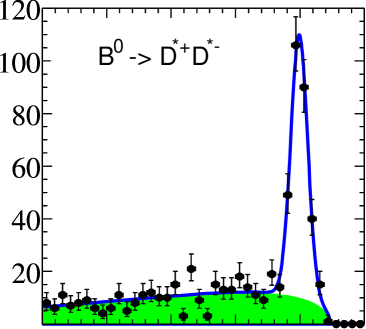
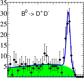
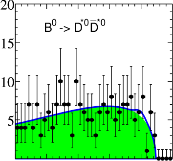
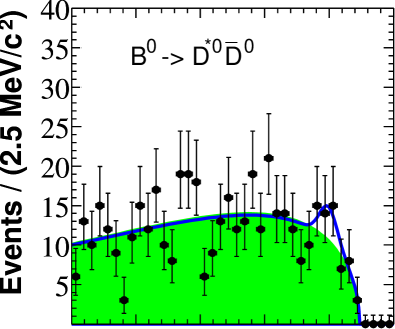
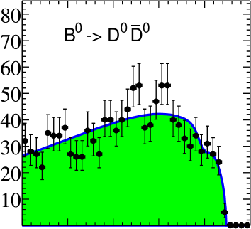
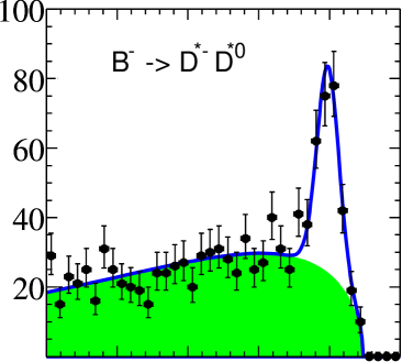
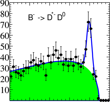
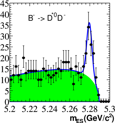
Figure 4: Distributions of $m_{\rm ES}$ for selected candidates in each $D^{(*)}\kern 1.99997pt\overline{\kern-1.99997ptD}{}^{(*)}$ mode. The error bars represent the statistical errors only. The solid lines represent the fits to the data, and the shaded areas the fitted background.

Table 7: Results of the fits for the ten signal decay modes: the number of events for fitted signal $N^{\rm sig}$, the peaking background $P$, and the crossfeed $C$, the branching fractions $\mathcal{B}$, 90% C.L. upper limits on branching fractions, previous measurements of branching fractions (for modes that have previous measurements), and charge asymmetries. The uncertainties are statistical. For the final branching fraction and charge asymmetry results, the systematic errors are also given.

Mode	$N^{\rm sig}$		$P$		$C$		$\mathcal{B}$ $(10^{-4})$			$\begin{array}[]{c}\mbox{{U.L.}}\\ (10^{-4})\end{array}$	$\begin{array}[]{c}\mbox{Previous $\mathcal{B}$}\\ \mbox{results $(10^{-4})$}\end{array}$	$\mathcal{A}_{C\!P}$
$B^{0}$ $\rightarrow D^{*+}D^{*-}$	270$\pm$	19	$-1$$\pm$	2	4$\pm$	1	$8.1$	$\pm 0.6\pm$	$1.0$		$\begin{array}[]{c}8.1\pm 0.8\pm 1.1\;[21]\\ 8.3\pm 1.6\pm 1.2\;[22]\\ 9.9^{+4.2}_{-3.3}\pm 1.2\;[23]\end{array}$
$B^{0}$ $\rightarrow D^{*\pm}D^{\mp}$	156$\pm$	17	1$\pm$	3	2$\pm$	1	$5.7$	$\pm 0.7\pm$	$0.7$		$\begin{array}[]{c}8.8\pm 1.0\pm 1.3\;[24]\\ 11.7\pm 2.6^{+2.2}_{-2.5}\;[25]\\ 6.7^{+2.0}_{-1.7}\pm 1.1\;[26]\end{array}$	$\quad 0.03\pm 0.10\pm 0.02\;\mbox{[27]}$
$B^{0}$ $\rightarrow D^{+}D^{-}$	63$\pm$	9	1$\pm$	2	0$\pm$	0	$2.8$	$\pm 0.4\pm$	$0.5$		$1.91\pm 0.51\pm 0.30\;[28]$
$B^{0}$ $\rightarrow D^{*0}\kern 1.99997pt\overline{\kern-1.99997ptD}{}^{*0}$	0$\pm$	6	$-2$$\pm$	2	0$\pm$	0	$-1.3$	$\pm 1.1\pm$	$0.4$	$0.9$	$<270$ Aleph1
$B^{0}$ $\rightarrow D^{*0}\kern 1.99997pt\overline{\kern-1.99997ptD}{}^{0}$	10$\pm$	8	$-2$$\pm$	3	1$\pm$	1	$1.0$	$\pm 1.1\pm$	$0.4$	$2.9$
$B^{0}$ $\rightarrow D^{0}\kern 1.99997pt\overline{\kern-1.99997ptD}{}^{0}$	$-11$$\pm$	12	$-8$$\pm$	4	0$\pm$	0	$-0.1$	$\pm 0.5\pm$	$0.2$	$0.6$
$B^{+}$ $\rightarrow D^{*+}\kern 1.99997pt\overline{\kern-1.99997ptD}{}^{*0}$	185$\pm$	20	$-5$$\pm$	4	34$\pm$	4	$8.1$	$\pm 1.2\pm$	$1.2$		$\begin{array}[]{c}10.5^{+3.3}_{-2.8}\pm 2.0\;[26]\\ <110\;[29]\end{array}$	$-0.15\pm 0.11\pm 0.02$
$B^{+}$ $\rightarrow D^{*+}\kern 1.99997pt\overline{\kern-1.99997ptD}{}^{0}$	115$\pm$	16	1$\pm$	4	3$\pm$	1	$3.6$	$\pm 0.5\pm$	$0.4$		$\begin{array}[]{c}4.57\pm 0.71\pm 0.56\;[28]\\ <130\;[29,30]\end{array}$	$-0.06\pm 0.13\pm 0.02$
$B^{+}$ $\rightarrow D^{+}\kern 1.99997pt\overline{\kern-1.99997ptD}{}^{*0}$	63$\pm$	11	3$\pm$	3	9$\pm$	2	$6.3$	$\pm 1.4\pm$	$1.0$		$<130$ Aleph1 ; Aleph1N	$0.13\pm 0.18\pm 0.04$
$B^{+}$ $\rightarrow D^{+}\kern 1.99997pt\overline{\kern-1.99997ptD}{}^{0}$	129$\pm$	20	$-2$$\pm$	5	1$\pm$	1	$3.8$	$\pm 0.6\pm$	$0.5$		$\begin{array}[]{c}4.83\pm 0.78\pm 0.58\;[28]\\ <67\;[29]\end{array}$	$-0.13\pm 0.14\pm 0.02$

We then fit the actual data to determine the number of reconstructed signal events in each mode. We fit the $m_{\rm ES}$ distributions of reconstructed $B$ decays that pass all selection criteria in each mode $i$ to a sum of a Gaussian distribution and a phase space distribution (Eq. 5), similar to the PDFs used for efficiency and peaking background fits described above. We minimize the $\chi^{2}_{i}$ of each data fit, allowing the parameter $\kappa_{i}$, the number of signal events in data $N^{\rm sig}_{i}$, and the number of background events in data $N^{\rm bkg}_{i}$, each to float. The $m_{\rm ES}$ distributions and the results of the fits are shown in Fig. 4. The branching fractions $\mathcal{B}_{i}$ are then determined via the equation

$$\sum_{j}\epsilon_{ij}\mathcal{B}_{j}N_{B}=N^{\rm sig}_{i}-P_{i}$$ (6)

where $N_{B}=N_{B\kern 1.25995pt\overline{\kern-1.25995ptB}{}}=(231.7\pm 2.6)\times 10^{6}$ is the total number of charged or neutral $B$ decays in the data sample, assuming equal production rates of charged and neutral $B$ pairs.

We determine the branching fractions as

$$\mathcal{B}_{i}=\sum_{j}\epsilon^{-1}_{ij}(N^{\rm sig}_{j}-P_{j})/N_{B},$$ (7)

(where $\epsilon^{-1}_{ij}$ is the inverse of matrix $\epsilon_{ij}$) yields the branching fractions given in Table 7. Note that the measured branching fractions for the three modes $B^{0}\rightarrow D^{(*)0}\kern 1.99997pt\overline{\kern-1.99997ptD}{}^{(*)0}$ are not significantly greater than zero. Thus, we have determined upper limits on the branching fractions for these modes. The 90% confidence level (C.L.) upper limits quoted in Table 7 are determined using the Feldman-Cousins method FeldmanCousins and include all systematic uncertainties detailed below. Since the branching fractions can be correlated through the use of Eq. 6, we also provide the covariance matrix, with all systematic uncertainties included, in Table 8. The covariance matrix is obtained via the approximation given in matinverr .

Table 8: Covariances of $B\rightarrow D^{(*)}\bar{D}^{(*)}$ branching fractions (with all systematic uncertainties included), in units of $10^{-8}$.

Mode	$D^{*+}D^{*-}$	$D^{*\pm}D^{\mp}$	$D^{+}D^{-}$	$D^{*0}\kern 1.99997pt\overline{\kern-1.99997ptD}{}^{*0}$	$D^{*0}\kern 1.99997pt\overline{\kern-1.99997ptD}{}^{0}$	$D^{0}\kern 1.99997pt\overline{\kern-1.99997ptD}{}^{0}$	$D^{*+}\kern 1.99997pt\overline{\kern-1.99997ptD}{}^{*0}$	$D^{*+}\kern 1.99997pt\overline{\kern-1.99997ptD}{}^{0}$	$D^{+}\kern 1.99997pt\overline{\kern-1.99997ptD}{}^{*0}$	$D^{+}\kern 1.99997pt\overline{\kern-1.99997ptD}{}^{0}$
$D^{*+}D^{*-}$	1.26	0.55	0.22	$-$0.15	0.07	$-$0.01	0.73	0.33	0.54	0.30
$D^{*\pm}D^{\mp}$		0.91	0.26	$-$0.08	0.04	$-$0.01	0.46	0.19	0.37	0.26
$D^{+}D^{-}$			0.39	$-$0.03	0.02	0.00	0.16	0.08	0.26	0.16
$D^{*0}\kern 1.99997pt\overline{\kern-1.99997ptD}{}^{*0}$				1.27	$-$0.04	0.00	$-$0.53	$-$0.06	$-$0.13	$-$0.05
$D^{*0}\kern 1.99997pt\overline{\kern-1.99997ptD}{}^{0}$					1.25	0.00	0.07	$-$0.02	0.05	0.02
$D^{0}\kern 1.99997pt\overline{\kern-1.99997ptD}{}^{0}$						0.22	$-$0.01	0.00	$-$0.01	0.00
$D^{*+}\kern 1.99997pt\overline{\kern-1.99997ptD}{}^{*0}$							2.60	0.31	0.55	0.27
$D^{*+}\kern 1.99997pt\overline{\kern-1.99997ptD}{}^{0}$								0.43	0.19	0.11
$D^{+}\kern 1.99997pt\overline{\kern-1.99997ptD}{}^{*0}$									2.61	0.27
$D^{+}\kern 1.99997pt\overline{\kern-1.99997ptD}{}^{0}$										0.53

VI Branching fraction systematic uncertainties

Table 9: Estimates of branching fraction systematic uncertainties (as percentages of the absolute values of the branching fraction central values) for all $B$ modes, after propagating the errors through Eq. 6. The totals are the sums in quadrature of the uncertainties in each column. Note that the term “Dalitz weight” refers to the selection on the reconstructed invariant masses of the $K^{-}\pi^{+}$ and $K^{-}\pi^{0}$ pairs for $D^{0}\rightarrow K^{-}\pi^{+}\pi^{0}$ decays that was described in Sec. III.4.

Mode	$D^{*+}D^{*-}$	$D^{*\pm}D^{\mp}$	$D^{+}D^{-}$	$D^{*0}\kern 1.79997pt\overline{\kern-1.79997ptD}{}^{*0}$	$D^{*0}\kern 1.79997pt\overline{\kern-1.79997ptD}{}^{0}$	$D^{0}\kern 1.79997pt\overline{\kern-1.79997ptD}{}^{0}$	$D^{*+}\kern 1.79997pt\overline{\kern-1.79997ptD}{}^{*0}$	$D^{*+}\kern 1.79997pt\overline{\kern-1.79997ptD}{}^{0}$	$D^{+}\kern 1.79997pt\overline{\kern-1.79997ptD}{}^{*0}$	$D^{+}\kern 1.79997pt\overline{\kern-1.79997ptD}{}^{0}$
$D^{*+}$ BFs	1.4	0.7	0.0	0.9	0.1	0.0	0.7	0.7	0.0	0.0
$D^{*0}$ BFs	0.0	0.0	0.0	4.9	1.6	0.0	2.1	0.0	4.4	0.0
$D^{0}$ BFs	5.0	2.7	0.0	7.4	3.7	5.7	5.2	4.5	3.3	2.7
$D^{+}$ BFs	1.4	6.5	13.2	0.1	0.2	0.4	0.1	0.3	6.5	6.5
Tracking efficiency	7.9	6.5	4.8	7.9	3.0	4.7	6.0	6.0	3.8	4.4
$K^{0}_{\scriptscriptstyle S}$ efficiency	0.3	0.2	0.0	0.0	0.1	0.0	0.1	0.2	0.3	0.2
Neutrals efficiency	2.5	1.0	0.0	8.4	2.9	1.9	4.6	1.6	4.3	1.0
Kaon identification	4.6	4.7	5.0	7.3	4.9	5.4	5.0	4.6	4.6	4.7
${\cal L}_{\rm Mass}$ cut	1.1	1.1	1.1	1.1	1.1	1.1	1.1	1.1	1.1	1.1
$\cal{F}$ cut	0.0	0.0	0.9	0.9	0.9	0.9	0.9	0.9	0.9	0.9
$L$ cut	0.0	0.0	0.8	0.8	0.8	0.8	0.0	0.8	0.8	0.8
$\Delta E$ cut	1.1	1.1	1.1	1.1	1.1	1.1	1.1	1.1	1.1	1.1
Dalitz weight cut	1.0	0.5	0.0	1.4	0.2	1.0	1.0	0.8	0.7	0.5
P($\chi^{2}$) cut	3.8	3.8	3.8	3.8	3.8	3.8	3.8	3.8	3.8	3.8
Fit model	1.8	3.6	3.1	5.4	6.7	44.6	4.9	2.8	7.0	3.6
Spin alignment	1.0	0.0	0.0	6.1	0.0	0.1	4.1	0.0	0.0	0.0
Peaking background	0.9	2.0	2.9	24.5	32.3	144.6	3.1	3.4	4.9	4.0
Crossfeed	0.4	0.6	0.8	1.9	1.1	1.6	0.6	0.4	1.0	0.6
$N_{B\kern 1.13394pt\overline{\kern-1.13394ptB}{}}$	1.1	1.1	1.1	1.1	1.1	1.1	1.1	1.1	1.1	1.1
Total	12.0	12.3	16.1	31.0	34.2	151.7	13.6	11.0	14.8	11.9

Table 9 shows the results of our evaluation of the systematic uncertainties on the branching fraction measurements.

Submode branching fractions

The central values and uncertainties on the branching fractions of the $D$ and $D^{*}$ mesons are propagated into the calculation of the branching fraction measurements. The world average measurements PDG2004 are used.

Charged track finding efficiency

From studies of absolute tracking efficiency, we assign a systematic uncertainty of 0.8% per charged track on the efficiency of finding tracks other than slow pions from charged $D^{*}$ decays and daughters of $K^{0}_{\scriptscriptstyle S}$ decays. For the slow pions, we assign a systematic uncertainty of 2.2% each, as determined from a separate efficiency study (using extrapolation of slow tracks found in the SVT into the DCH tracking detector and vice-versa). Track finding efficiency uncertainties are treated as 100% correlated among the tracks in a candidate. These uncertainties are weighted by the $D$ and $D^{*}$ branching fractions.

$K^{0}_{\scriptscriptstyle S}$ reconstruction efficiency

From a study of the $K^{0}_{\scriptscriptstyle S}$ reconstruction efficiency (using an inclusive data sample of events containing one or more $K^{0}_{\scriptscriptstyle S}$, as well as corresponding MC samples), we assign a 2.5% systematic uncertainty for all modes containing a $K^{0}_{\scriptscriptstyle S}$. The value 2.5% comes from the statistical uncertainty in the ratio of data to MC yields and the variation of this ratio over different selection criteria. The uncertainty is weighted by the $D$ and $D^{*}$ branching fractions.

$\pi^{0}$ and $\gamma$ finding efficiency

From studies of the neutral particle finding efficiency through the ratios of $\tau^{+}\rightarrow\rho^{+}(\pi^{+}\pi^{0})\nu$ to $\tau^{+}\rightarrow\pi^{+}\nu$ between data and MC, we assign a 3% systematic uncertainty per $\pi^{0}$, including the slow $\pi^{0}$ from $D^{*}$ and $D^{*0}$ decays. For isolated photons from $D^{*0}$ decays, we assign a 1.8% systematic uncertainty, 100% correlated with the $\pi^{0}$ efficiency uncertainty. These uncertainties are weighted by the $D$ and $D^{*}$ branching fractions.

Charged kaon identification

We assign a systematic uncertainty of 2.5% per charged kaon, according to a study of kaon particle identification efficiency (using kinematically-reconstructed $D^{0}\rightarrow K^{-}\pi^{+}$ candidates). The uncertainty is weighted by the $D$ and $D^{*}$ branching fractions.

Other selection differences between data and MC

Differences in momentum measurement, decay vertex finding efficiency, etc., can result in additional differences between efficiencies in data and in MC. We use a sample of the more abundant $B^{0}\rightarrow D_{s}^{*+}D^{*-}$ events in data, selected in a similar manner as the $B\rightarrow D^{(*)}\kern 1.99997pt\overline{\kern-1.99997ptD}{}^{(*)}$ modes, to determine these uncertainties. To estimate the systematic error arising from differences between the data and MC $D$ and $D^{*}$ mass resolutions, we calculate the number of $D_{s}^{*}D^{*}$ events seen in the data and MC as a function of the ${\cal L}_{\rm Mass}$ cut, while fixing the other selection criteria to their nominal values. The number of observed events is extracted from a fit to the $m_{\rm ES}$ distribution. We then plot the ratio of the data yield ($N_{\rm data}$) to the MC yield ($N_{\rm MC}$) as a function of the ${\cal L}_{\rm Mass}$ cut over a range of values that gives the same efficiencies as in the $D^{(*)}\kern 1.99997pt\overline{\kern-1.99997ptD}{}^{(*)}$ analyses. We find the rms of the $N_{\rm data}/N_{\rm MC}$ ratio and assign this as a systematic uncertainty for applying this cut. The same technique is used to determine the systematic uncertainties from all other selection criteria in Table 9: the selections on $\cal{F}$, $L$, $\Delta E$, the reconstructed invariant masses for $D^{0}\rightarrow K^{-}\pi+\pi^{0}$ (“Dalitz weight”), and vertex P($\chi^{2}$).

Fit model

The data yield is obtained from an $m_{\rm ES}$ fit where the mean ($\mu$) and width ($\sigma$) of the $B$ mass and the end-point ($\sqrt{s}/2$) of the phase-space distribution (Eq. 5) are fixed. These parameters are estimated and have associated uncertainties. The nominal value of $\sigma$ is determined from signal MC for each $B$ decay mode. To estimate the systematic uncertainty due to possible differences between the $m_{\rm ES}$ resolutions in data and signal MC, we first look at this difference ($\Delta\sigma=\sigma_{\rm data}-\sigma_{\rm MC}$) for those modes with high purity, including our control sample. These differences are consistent with zero, justifying our use of $\sigma_{\rm MC}$ in obtaining the data yield. We then find the weighted average of $\Delta\sigma$, which is given by $(0.11\pm 0.08)$ ${\mathrm{\,Me\kern-1.00006ptV\!/}c^{2}}$. As a conservative estimate, we repeat the data yield determinations by moving $\sigma$ up and down by 0.2 ${\mathrm{\,Me\kern-1.00006ptV\!/}c^{2}}$, and take the average of the absolute values of the changes in each data yield as the systematic uncertainty of fixing $\sigma$ to the MC value for that $B$ mode. A combined fit of common modes in data is used to determine the nominal values for $\mu$ and for the endpoint of the $m_{\rm ES}$ distribution $\sqrt{s}/2$. Hence, we move the parameters up and down by their fitted errors (0.2 ${\mathrm{\,Me\kern-1.00006ptV\!/}c^{2}}$ for $\mu$ and 0.1 ${\mathrm{\,Me\kern-1.00006ptV\!/}c^{2}}$ for $\sqrt{s}/2$) to obtain their corresponding systematic uncertainties. The quadratic sum of the three uncertainties from $\mu$, $\sigma$ and $\sqrt{s}/2$ gives the systematic uncertainty of the fit model for each $B$ mode.

Spin-alignment dependence

The $B^{0}\rightarrow D^{*+}D^{*-}$, $B^{0}\rightarrow D^{*0}\kern 1.99997pt\overline{\kern-1.99997ptD}{}^{*0}$, and $B^{+}\rightarrow\kern 1.99997pt\overline{\kern-1.99997ptD}{}^{*0}D^{*+}$ decays are pseudoscalar $\rightarrow$ vector vector (VV) transitions described by three independent helicity amplitudes $A_{0}$, $A_{\parallel}$, and $A_{\perp}$ Dunietz . The lack of knowledge of the true helicity amplitudes in the $B\rightarrow VV$ final states contributes a systematic uncertainty to the efficiency. The dominant source of this effect originates from the $p_{T}$-dependent inefficiency in reconstructing the low-momentum “soft” pions in the $D^{*+}$ and $D^{*0}$ decays, and the fact that the three helicity amplitudes contribute very differently to the slow pion $p_{T}$ distributions. To estimate the size of this effect, MC samples are produced with a phase-space angular distribution model for the decay products. Each event is then weighted by the angular distribution for given input values of the helicity amplitudes and phase differences. The efficiency is then determined for a large number of amplitude sets and the observed distributions in efficiencies are used to estimate a systematic uncertainty. For a given iteration, a random number, based on a uniform PDF, is generated for each of the three parameters: $R_{\perp},\alpha$, and $\eta$, where

$$\!R_{\perp}=\frac{|A_{\perp}|^{2}}{|A_{0}|^{2}+|A_{\parallel}|^{2}+|A_{\perp}|^{2}},\quad\alpha=\frac{|A_{0}|^{2}-|A_{\parallel}|^{2}}{|A_{0}|^{2}+|A_{\parallel}|^{2}},$$ (8)

and $\eta$ is the strong phase difference between $A_{0}$ and $A_{||}$. Since $R_{\perp}$ for $B^{0}\rightarrow D^{*+}D^{*-}$ has already been measured babarDstDstCP , a Gaussian PDF with mean and width fixed to the measured values is used instead for that mode. The events of the MC sample are weighted by the corresponding angular distribution and the efficiency is determined (after applying all selection cuts) by fitting the $m_{\rm ES}$ distribution and dividing by the number of generated events. The procedure is repeated 1000 times for each $B\rightarrow VV$ sample. The relative spread in efficiencies (rms divided by the mean) is used to estimate the systematic uncertainty due to a lack of knowledge of the true amplitudes.

Peaking background and crossfeed

The uncertainties on the peaking background vector $P_{i}$ and on the efficiency matrix $\epsilon_{ij}$ are dominated by the available MC statistics. The resulting uncertainties on each element of the vector and matrix are propagated through to the branching fraction results via the formalism of Eq. 6.

Number of $B\kern 1.79993pt\overline{\kern-1.79993ptB}{}$

The number of $B\kern 1.79993pt\overline{\kern-1.79993ptB}{}$ events in the full data sample, and the uncertainty on this number, are determined via a dedicated analysis of charged track multiplicity and event shape FoxW . The uncertainty introduces a systematic uncertainty of 1.1% on each of the branching fractions.

VII Measurement of $C\!P$-violating charge asymmetries

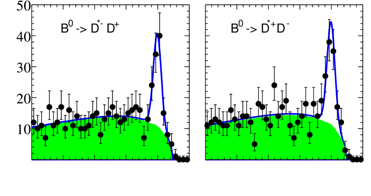
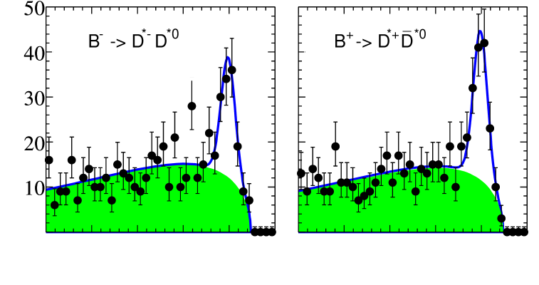
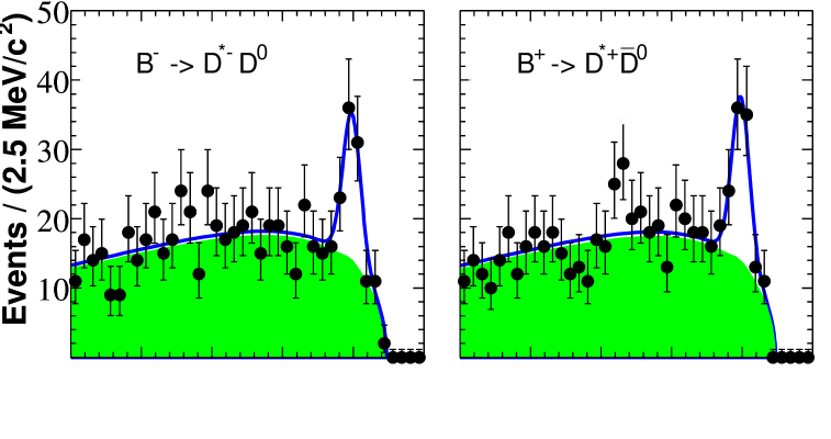
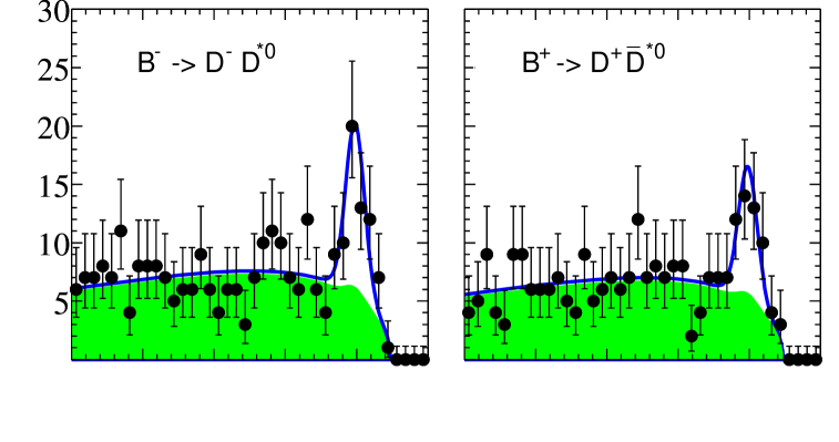
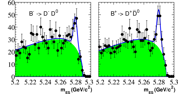
Figure 5: Fitted distributions of $m_{\rm ES}$ for the two conjugate states of each of the five relevant modes. The error bars represent the statistical errors only. The solid lines represent the fits to the data, and the shaded areas the fitted background. The raw asymmetries $\mathcal{A}$ are the normalized differences in the amount of signal between the members of each conjugate pair.

To obtain the charge asymmetries $\mathcal{A}_{C\!P}$ (defined in Eq. 1), we perform unbinned extended maximum likelihood fits to the $m_{\rm ES}$ distributions of the selected events in each of the four charged-$B$ decay modes $D^{*+}\kern 1.99997pt\overline{\kern-1.99997ptD}{}^{*0}$, $D^{*+}\kern 1.99997pt\overline{\kern-1.99997ptD}{}^{0}$, $D^{+}\kern 1.99997pt\overline{\kern-1.99997ptD}{}^{*0}$, $D^{+}\kern 1.99997pt\overline{\kern-1.99997ptD}{}^{0}$, and their respective charge conjugates, and in the neutral-$B$ decay mode $D^{*\pm}D^{\mp}$, using Eq. 5 as the PDF for the combinatorial background for both charges in each pair. The free parameters of each of the five fits individually are: 1) the combinatorial background shape parameter $\kappa$, 2) the total number of signal events, 3) the total number of background events, and 4) the “raw” charge asymmetry $\mathcal{A}$. Parameters 1 and 3 are considered (and thus constrained to be) the same for both charge states in each mode; this assumption is validated in MC simulation of the background as well as in control samples of $B^{0}\rightarrow D^{*-}\rho^{+}$ and $B^{0}\rightarrow D^{*-}a_{1}^{+}$ decays in data. The results of the fits are shown in Fig. 5. Two potentially biasing effects must be considered: there can be a asymmetry in the efficiencies for reconstructing positively- and negatively-charged tracks, and peaking background and crossfeed between the modes can cause a small difference between the measured (“raw”) asymmetry and the true asymmetry. The former of those two effects is discussed in Sec. VIII below. Regarding the latter, to obtain the charge asymmetries $\mathcal{A}_{C\!P}$ from the “raw” asymmetries $\mathcal{A}$, very small corrections for peaking background and crossfeed between modes must be made. Using the terminology of Eq. 6, and considering the branching fractions $\mathcal{B}_{i}$ to be sums of a “$+$” mode (with a $B^{0}$ or $B^{+}$, containing a $\bar{b}$ quark, as the initial state) and a “$-$” mode (with a $\kern 1.79993pt\overline{\kern-1.79993ptB}{}^{0}$ or $B^{-}$, which contain a $b$ quark, as the initial state): $\mathcal{B}_{i}\equiv\mathcal{B}_{i}^{+}+\mathcal{B}_{i}^{-}$, we have the two equations

$$\sum_{j}\epsilon_{ij}\mathcal{B}_{j}^{\pm}N_{B}=N^{\rm sig\pm}_{i}-P_{i}^{\pm}$$ (9)

for the “$+$” and “$-$” states respectively, which imply

$$\mathcal{B}_{i}^{-}\pm\mathcal{B}_{i}^{+}=$$

$$\qquad\sum_{j}\epsilon^{-1}_{ij}[(N^{\rm sig-}_{j}-P_{j}^{-})\pm(N^{\rm sig+}_{j}-P_{j}^{+})]/N_{B}.\qquad$$ (10)

As

$$\mathcal{A}_{C\!P,i}\equiv\frac{\Gamma_{i}^{-}-\Gamma_{i}^{+}}{\Gamma_{i}^{-}+\Gamma_{i}^{+}}=\frac{\mathcal{B}_{i}^{-}-\mathcal{B}_{i}^{+}}{\mathcal{B}_{i}^{-}+\mathcal{B}_{i}^{+}},$$ (11)

we have

$$\mathcal{A}_{C\!P,i}=\frac{\sum_{j}\epsilon^{-1}_{ij}[(N^{\rm sig-}_{j}-P_{j}^{-})-(N^{\rm sig+}_{j}-P_{j}^{+})]}{\sum_{j}\epsilon^{-1}_{ij}[(N^{\rm sig-}_{j}-P_{j}^{-})+(N^{\rm sig+}_{j}-P_{j}^{+})]}.$$ (12)

Since $N^{\rm sig}_{j}\equiv N^{\rm sig-}_{j}+N^{\rm sig+}_{j}$ and the “raw” asymmetry in a mode $\mathcal{A}_{j}\equiv\frac{N^{\rm sig-}_{j}-N^{\rm sig+}_{j}}{N^{\rm sig-}_{j}+N^{\rm sig+}_{j}}$, we have

$$\mathcal{A}_{C\!P,i}=\frac{\sum_{j}\epsilon^{-1}_{ij}[\mathcal{A}_{j}N^{\rm sig}_{j}-\mathcal{A}^{P}_{j}P_{j}]}{\sum_{j}\epsilon^{-1}_{ij}[N^{\rm sig}_{j}-P_{j}]}$$ (13)

where $\mathcal{A}^{P}_{j}\equiv\frac{P_{j}^{-}-P_{j}^{+}}{P_{j}^{-}+P_{j}^{+}}$ are the charge asymmetries of the peaking backgrounds. The total yields $N^{\rm sig}_{j}$, peaking backgrounds $P_{j}$, and efficiency matrix $\epsilon_{ij}$ are identical to those used for the branching fraction measurements and are given in Tables 7 and 6. The values $\mathcal{A}^{P}_{j}$ are nominally set to 0 and are varied to obtain systematic uncertainties due to the uncertainty on the charge asymmetry of the peaking background (see Sec. VIII). Thus, Eq. 13 is used to determine the final $\mathcal{A}_{C\!P}$ values from the measured asymmetries, in order to account for the small effects due to peaking background and crossfeed between modes. The measured $\mathcal{A}_{C\!P}$ values are given in Table 7. They are all consistent with zero, and their errors are dominated by statistical uncertainty.

Table 10: Summary of the systematic uncertainties estimated for the $\mathcal{A}_{C\!P}$ asymmetries, in %.

Systematics source	$B^{0}\rightarrow D^{*\pm}D^{\mp}$	$B^{+}\rightarrow D^{*+}\kern 1.99997pt\overline{\kern-1.99997ptD}{}^{*0}$	$B^{+}\rightarrow D^{*+}\kern 1.99997pt\overline{\kern-1.99997ptD}{}^{0}$	$B^{+}\rightarrow D^{+}\kern 1.99997pt\overline{\kern-1.99997ptD}{}^{*0}$	$B^{+}\rightarrow D^{+}\kern 1.99997pt\overline{\kern-1.99997ptD}{}^{0}$
Slow pion charge asymmetry	$0.53$	$0.53$	$0.53$	—	—
Charge asymmetry from other tracks	$0.80$	$0.80$	$0.80$	$0.80$	$0.80$
Amount of peaking bkgd.	$0.06$	$0.42$	$0.19$	$0.64$	$0.53$
$\mathcal{A}_{C\!P}$ of peaking bkgd.	$0.42$	$0.09$	$0.58$	$3.36$	$0.85$
Crossfeed uncertainty	$0.00$	$0.00$	$0.01$	$0.31$	$0.00$
$m_{\rm ES}$ resolution uncertainty	$0.20$	$0.04$	$0.04$	$0.01$	$0.14$
$B$ mass uncertainty	$0.20$	$0.37$	$1.38$	$1.38$	$0.53$
Uncertainty in $\sqrt{s}$	$0.00$	$0.03$	$0.08$	$0.05$	$0.05$
Potential fit bias	$0.74$	$1.97$	$1.19$	$0.53$	$1.66$
TOTAL $\delta(\mathcal{A}_{C\!P})$	$1.6$	$2.4$	$2.3$	$3.8$	$2.2$

VIII Systematic uncertainties on charge asymmetry measurements

Table 10 shows the results of our evaluation of the various sources of systematic uncertainty that are important for the $\mathcal{A}_{C\!P}$ measurements.

Slow $\pi^{\pm}$ charge asymmetry

A charge asymmetry in the reconstruction efficiency of the low-transverse-momentum charged pions from $D^{*\pm}\rightarrow D^{0}\pi^{\pm}$ decays can cause a shift in $\mathcal{A}_{C\!P}$ by biasing the rates of positively charged vs. negatively charged decays for each mode. We estimate this systematic uncertainty by using data control samples of $B^{0}\rightarrow D^{*-}X^{+}$ and $\kern 1.79993pt\overline{\kern-1.79993ptB}{}^{0}\rightarrow D^{*+}X^{-}$ decays, where $X$ is either $\pi$, $\rho$, or $a_{1}$, and determining if there is an asymmetry in the number of $D^{*+}$ vs. $D^{*-}$ reconstructed. There are two potential biases of this technique: 1) a charge asymmetry in tracks other than the slow charged pions, and 2) the presence of doubly-Cabibbo-suppressed $B^{0}(\kern 1.79993pt\overline{\kern-1.79993ptB}{}^{0})\rightarrow D^{*\mp}X^{\pm}$ decays which could potentially introduce a direct-$C\!P$-violating asymmetry between the two states in the control sample. Discussion of 1) is detailed in the paragraph below, and the rate of 2) has been determined in analyses such as Refs. exclS2bg and partialS2bg to be of order $0.1\%$, well below the sensitivity for this measurement. We combine the information from the control sample modes and determine an uncertainty of 0.5% for each $\mathcal{A}_{C\!P}$ measurement for modes with a charged slow pion.

Charge asymmetry from tracks other than slow $\pi^{\pm}$

Auxilliary track reconstruction studies place a stringent bound on detector charge asymmetry effects at transverse momenta above 200 ${\mathrm{\,Me\kern-1.00006ptV\!/}c}$. Such tracking and PID systematic effects were studied in detail in the analysis of $B\rightarrow\phi K^{*}$ phikstar . We assign a 0.2% systematic per charged track, thus an overall systematic of 0.4% per mode (as the positively charged and negatively charged decays for each mode have, on balance, one positive vs. one negative track respectively). This systematic uncertainty is added linearly to the slow pion charge asymmetry systematic due to potential correlation.

Amount of peaking background

Peaking background can potentially bias $\mathcal{A}_{C\!P}$ measurements in two ways: 1) a difference in the total amount of peaking background from the expected total amount can, to second order, alter the measured asymmetry between the positively charged and negatively charged decays, 2) a more direct way for peaking background to alter the measured $\mathcal{A}_{C\!P}$ would be if the peaking background itself were to have an asymmetry between the amount that is reconstructed as positively charged and the amount reconstructed as negative. 1) is discussed here; 2) is discussed in the paragraph below. The systematic uncertainty due to the uncertainty on the total amount of peaking background in the five decays is determined via the formalism of Eq. 13. Namely, the uncertainty is given by

$$\delta\mathcal{A}_{C\!P,i}=\frac{(\sum_{j}\epsilon^{-1}_{ij}\mathcal{A}_{j}N^{\rm sig}_{j})\times\sqrt{\sum_{j}(\epsilon^{-1}_{ij})^{2}(\delta P)^{2}_{j}}}{(\sum_{j}\epsilon^{-1}_{ij}[N^{\rm sig}_{j}-P_{j}])^{2}}$$ (14)

where $(\delta P)_{j}$ are the uncertainties on the amount of peaking background (which are given, along with the other parameters in the equation, in Table 7).

$\mathcal{A}_{C\!P}$ of peaking background

The systematic uncertainty due to the $\mathcal{A}_{C\!P}$ of the peaking background is also determined using the formalism of Eq. 13. Namely, the uncertainty is given by

$$\!\!\!\!\delta^{\prime}\mathcal{A}_{C\!P,i}=\frac{(\sum_{j}\epsilon^{-1}_{ij}\mathcal{A}_{j}N^{\rm sig}_{j})\!\times\!\!\sqrt{\sum_{j}(\epsilon^{-1}_{ij})^{2}(\delta A^{P})^{2}_{j}P^{2}_{j}}}{(\sum_{j}\epsilon^{-1}_{ij}[N^{\rm sig}_{j}-P_{j}])(\sum_{j}\epsilon^{-1}_{ij}\mathcal{A}_{j}N^{\rm sig}_{j})}.$$ (15)

Investigation of the sources of the peaking background in these modes motivates a conservative choice of 0.68 for the $(\delta A^{P})_{j}$ values.

Amount of crossfeed

The systematic error due to uncertainties in the amount of crossfeed between the modes is also determined via the formalism of Eq. 13. Namely, the uncertainty is given by

$$\delta^{\prime\prime}\mathcal{A}_{C\!P,i} = \frac{\sqrt{\sum_{jk}\mathcal{A}_{j}N^{\rm sig}_{j}{\rm cov}(\epsilon^{-1}_{ij},\epsilon^{-1}_{ik})\mathcal{A}_{k}N^{\rm sig}_{k}}}{\sum_{j}\epsilon^{-1}_{ij}[N^{\rm sig}_{j}-P_{j}]}$$

$$\qquad-\quad\frac{(\sum_{j}\epsilon^{-1}_{ij}\mathcal{A}_{j}N^{\rm sig}_{j})\times(\sqrt{\sum_{jk}[N^{\rm sig}_{j}-P_{j}]{\rm cov}(\epsilon^{-1}_{ij},\epsilon^{-1}_{ik})[N^{\rm sig}_{k}-P_{k}]})}{(\sum_{j}\epsilon^{-1}_{ij}[N^{\rm sig}_{j}-P_{j}])^{2}}.$$

The covariance between the elements of the inverse efficiency matrix is obtained using the method of Ref. matinverr . The very small systematic uncertainty due to crossfeed is thus obtained using Eq. VIII and the amounts of crossfeed and their uncertainties that are given in Table 6.

Uncertainty in $m_{\rm ES}$ resolution, $B$ mass, and $\sqrt{s}$

The uncertainties in $m_{\rm ES}$ resolution and the beam energy $\sqrt{s}$ are determined by varying these parameters within their fitted $\pm 1\sigma$ ranges and observing the resulting changes in $\mathcal{A}_{C\!P}$. The uncertainty in the reconstructed $B$ mass can also have an impact on the fitted $m_{\rm ES}$ distributions and thus on the fitted $\mathcal{A}_{C\!P}$ values. Varying the $B$ mass between the fitted value and the $\pm 1\sigma$ range of the nominal $B^{0}$ or $B^{+}$ invariant mass allows the determination of the resulting effect on the $\mathcal{A}_{C\!P}$ values.

Potential fit bias

Uncertainties in the potential biases of the $\mathcal{A}_{C\!P}$ fits are determined by performing the fits on large samples of MC simulation of the signal decay modes and of $B\kern 1.79993pt\overline{\kern-1.79993ptB}{}$ and continuum background decays. All results are consistent with zero bias, and the uncertainties of the fitted asymmetries on the simulated data samples are conservatively assigned as systematic uncertainties from biases of the fits.

IX Implications for $\gamma$

Information on the weak phase $\gamma$ may be obtained by combining information from $B\rightarrow D^{(*)}\kern 1.99997pt\overline{\kern-1.99997ptD}{}^{(*)}$ and $B\rightarrow D^{(*)}_{s}\kern 1.99997pt\overline{\kern-1.99997ptD}{}^{(*)}$ branching fractions, along with $C\!P$ asymmetry measurements in $B\rightarrow D^{(*)}\kern 1.99997pt\overline{\kern-1.99997ptD}{}^{(*)}$, and using an SU(3) relation between the $D^{(*)}\kern 1.99997pt\overline{\kern-1.99997ptD}{}^{(*)}$ and $D^{(*)}_{s}\kern 1.99997pt\overline{\kern-1.99997ptD}{}^{(*)}$ decays DL ; ADL . For this analysis, we assume that the breaking of SU(3) can be parametrized via the ratios of decay constants $f_{D_{s}^{(*)}}/f_{D^{(*)}}$, which are quantities that can be determined either with lattice QCD or from experimental measurements lattice .

In this model, one obtains the relation (for $B^{0}\rightarrow D^{+}D^{-}$ and individual helicity states of $B^{0}\rightarrow D^{*+}D^{*-}$):

$$\mathcal{A}_{ct}^{2}=\frac{a_{R}\cos(2\beta+2\gamma)-a_{\rm indir}\sin(2\beta+2\gamma)-\mathcal{B}}{\cos 2\gamma-1}$$ (17)

where

$$\mathcal{B} \equiv \frac{1}{2}(|A^{D}|^{2}+|\bar{A}^{D}|^{2})=$$

$$\mathcal{A}_{ct}^{2}+\mathcal{A}_{ut}^{2}+2\mathcal{A}_{ct}\mathcal{A}_{ut}\cos\delta\cos\gamma,$$

$$a_{\rm dir} \equiv \frac{1}{2}(|A^{D}|^{2}-|\bar{A}^{D}|^{2})=$$

$$-2\mathcal{A}_{ct}\mathcal{A}_{ut}\sin\delta\sin\gamma,$$

$$a_{\rm indir} \equiv \Im[e^{-2i\beta}(A^{D})^{*}\bar{A}^{D}]=-\mathcal{A}_{ct}^{2}\sin 2\beta$$

$$-2\mathcal{A}_{ct}\mathcal{A}_{ut}\cos\delta\sin(2\beta+\gamma)$$

$$-\mathcal{A}_{ut}^{2}\sin(2\beta+2\gamma),$$

and

$$a_{R}^{2}\equiv\mathcal{B}^{2}-a_{\rm dir}^{2}-a_{\rm indir}^{2}.$$ (21)

$A^{D}$ and $\bar{A}^{D}$ represent amplitudes of a given $B^{0}$ and $\kern 1.79993pt\overline{\kern-1.79993ptB}{}^{0}\rightarrow D^{(*)+}D^{(*)-}$ decay respectively, $\mathcal{B}$ represents the corresponding average branching fraction, and $a_{\rm dir}$ and $a_{\rm indir}$ represent the corresponding direct and indirect $C\!P$ asymmetries respectively. The phases $\beta$ and $\gamma$ are the CKM phases and $\delta$ is a strong phase difference. $\mathcal{A}_{ct}\equiv|(T+E+P_{c}-P_{t}-P_{EW}^{C})V_{cb}^{*}V_{cd}|$ and $\mathcal{A}_{ut}\equiv|(P_{u}-P_{t}-P_{EW}^{C})V_{ub}^{*}V_{ud}|$ are the magnitudes of the combined $B\rightarrow D^{(*)}\kern 1.99997pt\overline{\kern-1.99997ptD}{}^{(*)}$ decay amplitudes containing $V_{cb}^{*}V_{cd}$ and $V_{ub}^{*}V_{ud}$ terms respectively, and the $T$, $P$, and $E$ terms are the tree, penguin, and the sum of exchange and annihilation amplitudes respectively DL . One can directly measure the parameters $\mathcal{B}$, $a_{\rm dir}$, and $a_{\rm indir}$ using information from $B\rightarrow D^{(*)}\kern 1.99997pt\overline{\kern-1.99997ptD}{}^{(*)}$ decays; the parameter $\mathcal{A}_{ct}$ using information from $B\rightarrow D^{(*)}_{s}\kern 1.99997pt\overline{\kern-1.99997ptD}{}^{(*)}$ decays; and the weak phase $\beta$ can be obtained from the measurements of $\sin 2\beta$ based on $B^{0}\rightarrow c\bar{c}K^{0}_{\scriptscriptstyle S}$ decays HFAG thus allowing for solution of $\gamma$ (up to two discrete ambiguities) via Eq. 17. As the vector-pseudoscalar modes $B^{0}\rightarrow D^{*\pm}D^{\mp}$ are not $C\!P$ eigenstates, a slightly more complicated analogue to Eq. 17 is needed for these modes ADL . Measurement of $\mathcal{A}_{C\!P}$ for $D^{*\pm}D^{\mp}$ is also necessary to obtain information on $\gamma$ from the vector-pseudoscalar modes.

Using these relations, there are four variables besides $\beta$ for each $B\rightarrow D^{(*)}\kern 1.99997pt\overline{\kern-1.99997ptD}{}^{(*)}$ decay for which to solve: $\mathcal{A}_{ct}$, $\mathcal{A}_{ut}$, $\delta$, and $\gamma$. The branching fraction and the direct and indirect $C\!P$ asymmetries of the $B\rightarrow D^{(*)}\kern 1.99997pt\overline{\kern-1.99997ptD}{}^{(*)}$ decay provide three measured quantities. The other measurement that can be used is the branching fraction of the corresponding $B\rightarrow D^{(*)}_{s}\kern 1.99997pt\overline{\kern-1.99997ptD}{}^{(*)}$ decay, by using the relation expressed in Eq. 22.

The values $a_{\rm indir}$ can, of course, only be measured in the neutral $B\rightarrow D^{(*)}\kern 1.99997pt\overline{\kern-1.99997ptD}{}^{(*)}$ decays. However, the charged $B\rightarrow D^{(*)}\kern 1.99997pt\overline{\kern-1.99997ptD}{}^{(*)}$ decays can supplement the neutral decays by adding information on $\mathcal{B}$ and $a_{\rm dir}$, assuming only isospin symmetry between the charged and neutral modes. Thus, information from the charged $B$ decay modes can assist the $\gamma$ determination.

SU(3)-breaking effects can distort the relation between $D^{(*)}\kern 1.99997pt\overline{\kern-1.99997ptD}{}^{(*)}$ and $D^{(*)}_{s}\kern 1.99997pt\overline{\kern-1.99997ptD}{}^{(*)}$ decays as expressed in Eq. 17. However, the SU(3)-breaking can be parametrized by the ratio of decay constants $f_{D_{s}^{(*)}}/f_{D^{(*)}}$, such that the amplitude for $B\rightarrow D^{(*)}_{s}\kern 1.99997pt\overline{\kern-1.99997ptD}{}^{(*)}$ decays

$$\mathcal{A}_{ct}^{\prime}=f_{D_{s}^{(*)}}/f_{D^{(*)}}\times\mathcal{A}_{ct}/\sin\theta_{c}$$ (22)

where $\theta_{c}$ is the Cabibbo angle PDG2004 and the parentheses around the asterisks correspond to the $B\rightarrow D^{(*)}\kern 1.99997pt\overline{\kern-1.99997ptD}{}^{(*)}$ and $B\rightarrow D^{(*)}_{s}\kern 1.99997pt\overline{\kern-1.99997ptD}{}^{(*)}$ decays that are used. The theoretical uncertainty of this relation is determined to be 10% DL .

We thus use the information from the vector-vector (VV) decays $B^{0}$ $\rightarrow D^{*+}D^{*-}$ and $B^{+}$ $\rightarrow D^{*+}\kern 1.99997pt\overline{\kern-1.99997ptD}{}^{*0}$ and pseudoscalar-pseudoscalar (PP) decays $B^{0}$ $\rightarrow D^{+}D^{-}$ and $B^{+}$ $\rightarrow D^{+}\kern 1.99997pt\overline{\kern-1.99997ptD}{}^{0}$, as well as the vector-pseudoscalar (VP) decays $B^{0}\rightarrow D^{*\pm}D^{\mp}$, $B^{+}\rightarrow D^{*+}\kern 1.99997pt\overline{\kern-1.99997ptD}{}^{0}$, and $B^{+}\rightarrow D^{+}\kern 1.99997pt\overline{\kern-1.99997ptD}{}^{*0}$, to form constraints on $\gamma$ using the method of Refs. DL ; ADL .

To use the VV decays, we must make the assumption that the strong phases for the $0$ and $\|$ helicity amplitudes are equal. The constraints from the PP decays require no such assumption. The assumption of equal $0$ and $\|$ helicity amplitudes is theoretically supported by a QCD factorization argument described in ADL . Then, using Eq. 17, we combine the $B^{0}$ $\rightarrow D^{*+}D^{*-}$ and $B^{+}$ $\rightarrow D^{*+}\kern 1.99997pt\overline{\kern-1.99997ptD}{}^{*0}$ branching fractions and $\mathcal{A}_{C\!P}$ information given above with measurements of the $B^{0}$ $\rightarrow D_{s}^{*-}D^{*+}$ and $B^{+}$ $\rightarrow D_{s}^{*+}\kern 1.99997pt\overline{\kern-1.99997ptD}{}^{*0}$ branching fractions PDG2004 , measurements of the $B^{0}$ $\rightarrow D^{*+}D^{*-}$ time-dependent $C\!P$ asymmetries babarDstDstCP ; Belle2 , and the world-average values of $\sin 2\beta$ HFAG and $\sin\theta_{c}$ PDG2004 .

We use a fast parametrized MC method, described in Ref. ADL , to determine the confidence intervals for $\gamma$. We consider 500 values for $\gamma$, evenly spaced between 0 and $2\pi$. For each value of $\gamma$ considered, we generate 25000 MC experiments, with inputs that are generated according to Gaussian distributions with widths equal to the experimental errors of each quantity. For each experiment, we generate random values of each of the experimental inputs according to Gaussian distributions, with means and sigmas according to the measured central value and total errors on each experimental quantity. We make the assumption that the ratio $f_{D_{s}^{*}}/f_{D^{*}}$ is equal to $f_{D_{s}}/f_{D}=1.20\pm 0.06\pm 0.06$ lattice , allowing for the additional 10% theoretical uncertainty DL . We then calculate the resulting values of $\mathcal{A}_{ct}$, $a_{\rm dir}$, $a_{\rm indir}$, and $B$, given the generated random values (based on the experimental values). When the quantities $a_{\rm dir}$, $a_{\rm indir}$, and $B$, along with $\beta$ and the value of $\gamma$ that is being considered, are input into Eq. (17), we obtain a residual value for each experiment, equal to the difference of the left- and right-hand sides of the equation. Thus, using Eq. 17, the 25000 trials per value of $\gamma$ provide an ensemble of residual values that are used to create a likelihood for $\gamma$ to be at that value, given the experimental inputs. The likelihood, as a function of $\gamma$, can be obtained from $\chi^{2}(\gamma)$, where $\chi^{2}\equiv(\mu/\sigma)^{2}$, $\mu$ is the mean of the above ensemble of residual values, and $\sigma$ is the usual square root of the variance. The value of $\chi^{2}(\gamma)$ is then considered to represent a likelihood which is equal to that of a value $\chi$ standard devations of a Gaussian distribution from the most likely value(s) of $\gamma$. We define the “exclusion level,” as a function of the value of $\gamma$, as follows: the value of $\gamma$ is excluded from a range at a given C.L. if the exclusion level in that range of $\gamma$ values is greater than the given C.L.

We now turn to the VP decays. The method using VP decays shares the advantage with PP decays that no assumptions on strong phases are required. The disadvantage is that, as we will see, the constraints from the VP modes are weak.

We combine the information given above on the $B^{0}$ $\rightarrow D^{*\pm}D^{\mp}$, $B^{+}\rightarrow D^{*+}\kern 1.99997pt\overline{\kern-1.99997ptD}{}^{0}$, and $B^{+}\rightarrow D^{+}\kern 1.99997pt\overline{\kern-1.99997ptD}{}^{*0}$ branching fractions and $\mathcal{A}_{C\!P}$ information with measurements of the $B^{0}$ $\rightarrow D_{s}^{*-}D^{+}$, $B^{0}$ $\rightarrow D_{s}^{-}D^{*+}$, $B^{+}$ $\rightarrow D_{s}^{*+}\kern 1.99997pt\overline{\kern-1.99997ptD}{}^{0}$, and $B^{+}$ $\rightarrow D_{s}^{+}\kern 1.99997pt\overline{\kern-1.99997ptD}{}^{*0}$ branching fractions PDG2004 , measurements of the $B^{0}$ $\rightarrow D^{*\pm}D^{\mp}$ time-dependent $C\!P$ asymmetries Babar2 ; belleDstDCP , and the world-average values of $\sin 2\beta$ HFAG and $\sin^{2}\theta_{c}$ PDG2004 . Similar to the MC $\gamma$ determination for the VV and PP modes, we generate random values of each of the experimental inputs according to Gaussian distributions, with means and sigmas according to the measured central value and total errors on each experimental quantity. We again obtain a confidence level distribution as a function of $\gamma$.

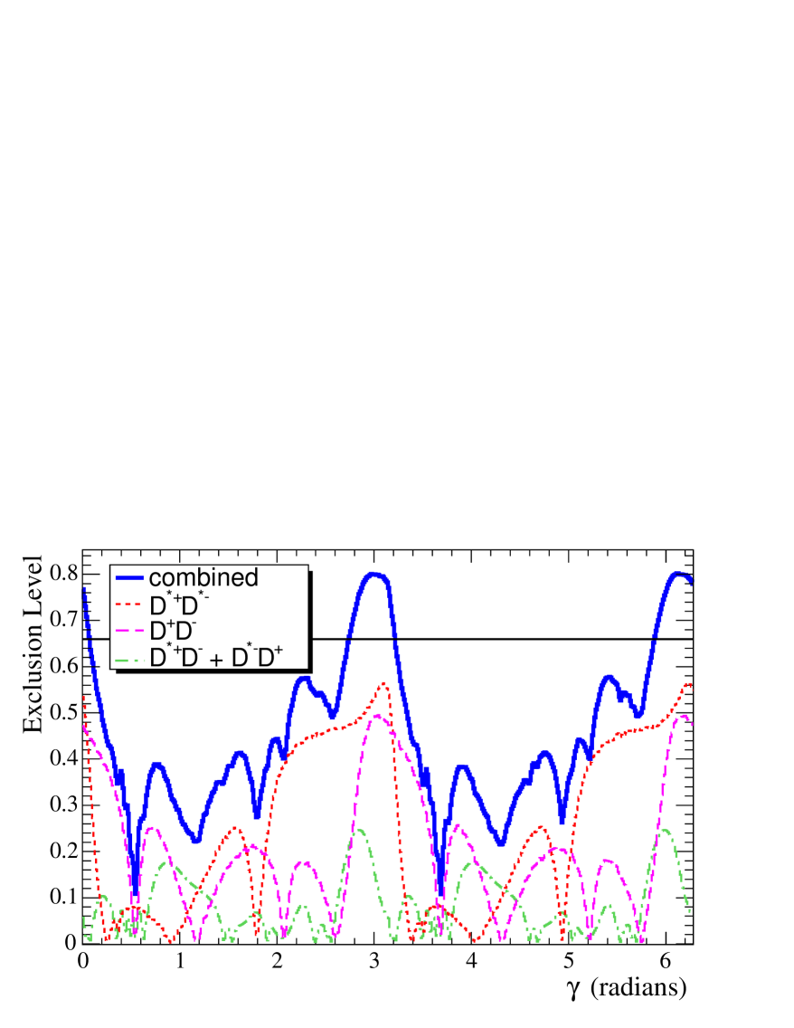
Figure 6: The measured exclusion level, as a function of $\gamma$, from the combined information from vector-vector, vector-pseudoscalar, and pseudoscalar-pseudoscalar modes. The combined information implies that $\gamma$ is favored to lie in the range $[0.07-2.77]$ radians (with a +0 or $+\pi$ radians ambiguity) radians at 68% confidence level.

Finally, we can combine information from the VV, PP, and VP modes. The resulting measured exclusion level as a function of $\gamma$ from each of the three sets of modes, as well as from their combination, is shown in Fig. 6. From the combined fit, we see that $\gamma$ is favored to lie in the range $[0.07-2.77]$ radians (with a +0 or $+\pi$ radians ambiguity) at 68% confidence level. This corresponds to $[4.1^{\circ}-158.6^{\circ}](+0^{\circ}\mbox{ or }180^{\circ})$.

These constraints are generally weaker than those found in Ref. ADL due to the fact that the measured $C\!P$ asymmetry in $B^{0}\rightarrow D^{*+}D^{*-}$ has moved closer to the world-average $\sin\!2\beta$, with the newer $B^{0}\rightarrow D^{*+}D^{*-}$ measurements in Ref. dstdst05prl . The closer this $C\!P$ asymmetry is to $\sin\!2\beta$, the weaker the resulting constraints are on $\gamma$, due to the fact that the closeness of the $C\!P$ asymmetry to $\sin\!2\beta$ favors the dominance of the tree amplitude, rather than the penguin amplitude whose phase provides the sensitivity to $\gamma$. Although the constraints are not strong, they contribute to the growing amount of information available on $\gamma$ from various sources.

X Conclusions

In summary, we have measured branching fractions, upper limits, and charge asymmetries for all $B$ meson decays to $D^{(*)}\kern 1.99997pt\overline{\kern-1.99997ptD}{}^{(*)}$. The results are shown in Table 7. This includes observation of the decay modes $B^{0}$ $\rightarrow D^{+}D^{-}$ and $B^{+}$ $\rightarrow D^{*+}\kern 1.99997pt\overline{\kern-1.99997ptD}{}^{*0}$, evidence for the decay modes $B^{+}$ $\rightarrow D^{+}\kern 1.99997pt\overline{\kern-1.99997ptD}{}^{*0}$ and $B^{+}$ $\rightarrow D^{+}\kern 1.99997pt\overline{\kern-1.99997ptD}{}^{0}$ at $3.8\sigma$ and $4.9\sigma$ levels respectively, constraints on $C\!P$-violating charge asymmetries in the four decay modes $B^{+}$ $\rightarrow D^{(*)+}\kern 1.99997pt\overline{\kern-1.99997ptD}{}^{(*)0}$, measurements of (and upper limits for) the decay modes $B^{0}$ $\rightarrow D^{*0}\kern 1.99997pt\overline{\kern-1.99997ptD}{}^{0}$ and $B^{0}$ $\rightarrow D^{0}\kern 1.99997pt\overline{\kern-1.99997ptD}{}^{0}$, and improved branching fractions, upper limits, and charge asymmetries in all other $B\rightarrow D^{(*)}\kern 1.99997pt\overline{\kern-1.99997ptD}{}^{(*)}$ modes. The results are consistent with theoretical expectation and (when available) previous measurements. When we combine information from time-dependent $C\!P$ asymmetries in $B^{0}\rightarrow D^{(*)+}D^{(*)-}$ decays dstdst05prl ; dstd05prl and world-averaged branching fractions of $B$ decays to $D_{s}^{(*)}\kern 1.99997pt\overline{\kern-1.99997ptD}{}^{(*)}$ modes PDG2004 using the technique proposed in Ref. DL and implemented in Ref. ADL , we find the CKM phase $\gamma$ is favored to lie in the range $[0.07-2.77]$ radians (with a +0 or $+\pi$ radians ambiguity) at 68% confidence level.

XI Acknowledgments

We are grateful for the extraordinary contributions of our PEP-II colleagues in achieving the excellent luminosity and machine conditions that have made this work possible. The success of this project also relies critically on the expertise and dedication of the computing organizations that support BABAR. The collaborating institutions wish to thank SLAC for its support and the kind hospitality extended to them. This work is supported by the US Department of Energy and National Science Foundation, the Natural Sciences and Engineering Research Council (Canada), Institute of High Energy Physics (China), the Commissariat à l’Energie Atomique and Institut National de Physique Nucléaire et de Physique des Particules (France), the Bundesministerium für Bildung und Forschung and Deutsche Forschungsgemeinschaft (Germany), the Istituto Nazionale di Fisica Nucleare (Italy), the Foundation for Fundamental Research on Matter (The Netherlands), the Research Council of Norway, the Ministry of Science and Technology of the Russian Federation, and the Particle Physics and Astronomy Research Council (United Kingdom). Individuals have received support from CONACyT (Mexico), the Marie-Curie Intra European Fellowship program (European Union), the A. P. Sloan Foundation, the Research Corporation, and the Alexander von Humboldt Foundation.

References

(1)
N. Cabibbo, Phys. Rev. Lett. 10, 531 (1963); M. Kobayashi and T. Maskawa, Prog. Theor. Phys. 49, 652 (1973).
(2)
M. Gronau, Phys. Rev. Lett. 63, 1451 (1989); Phys. Lett. B 233, 479 (1989);
R. Aleksan et al., Nucl. Phys. B 361, 141 (1991); Phys. Lett. B 317, 173 (1993).
(3)
J. Rosner, Phys. Rev. D 42, 3732 (1990).
(4)
A. I. Sanda and Z. Z. Xing, Phys. Rev. D 56, 341 (1997).
(5)
X. Y. Pham and Z. Z. Xing, Phys. Lett. B 458, 375 (1999).
(6)
Z. Z. Xing, Phys. Rev. D 61, 014010 (2000).
(7)
A. Datta and D. London, Phys. Lett. B 584, 81 (2004).
(8)
J. Albert, A. Datta, and D. London, Phys. Lett. B 605, 335 (2005).
(9)
J. Simone, Nucl. Phys. Proc. Suppl. 140, 443 (2005).
A value is found in the later
reference C. Aubin et al., Phys. Rev. Lett. 95, 122002 (2005); this value is
consistent within uncertainty to the prior value which we use.
One can also obtain information about the ratio of decay constants from
experiment, e.g. M. Artuso et al. (CLEO Collaboration),
Phys. Rev. Lett. 95, 251801 (2005).
(10)
Except as noted otherwise, throughout the article we use a particle name to denote either member of
a charge-conjugate pair.
(11)
B. Aubert et al. (BABAR Collaboration), Nucl. Instr. Methods Phys. Res., Sect. A 479, 1 (2002).
(13)
S. Agostinelli et al. (GEANT4 Collaboration), Nucl. Instr. Methods Phys. Res., Sect. A 506, 250 (2003).
(14)
Particle Data Group, S. Eidelman et al., Phys. Lett. B 592, 1 (2004).
(15)
G. C. Fox and S. Wolfram, Phys. Rev. Lett. 41, 1581 (1978).
(16)
R. H. Dalitz, Phil. Mag. 44, 1068 (1953).
(17)
D. Asner et al. (CLEO Collaboration), Phys. Rev. D 53, 1039 (1996).
(18)
H. Albrecht et al. (ARGUS Collaboration), Phys. Lett. B 241, 278 (1990);
ibid254, 288 (1991).
(19)
G. J. Feldman and R. D. Cousins, Phys. Rev. D 57, 3873 (1998).
(20)
M. Lefebvre et al., Nucl. Instr. Methods Phys. Res., Sect. A 451, 520 (2000).
(21)
H. Miyake et al. (Belle Collaboration), Phys. Lett. B 618, 34 (2005).
(22)
B. Aubert et al. (BABAR Collaboration), Phys. Rev. Lett. 89, 061801 (2002).
(23)
E. Lipeles et al. (CLEO Collaboration), Phys. Rev. D 62, 032005 (2000).
(24)
B. Aubert et al. (BABAR Collaboration), Phys. Rev. Lett. 90, 221801 (2003).
(25)
K. Abe et al. (Belle Collaboration), Phys. Rev. Lett. 89, 122001 (2002).
(26)
J. Albert, Ph.D. dissertation, Princeton Univ. (2002), SLAC-R-614.
(27)
Previous measurements for in are
, from B. Aubert et al. (BABAR Collaboration),
Phys. Rev. Lett. 90, 221801 (2003); and , from
T. Aushev et al. (Belle Collaboration), Phys. Rev. Lett. 93, 201802 (2004).
(28)
G. Majumder et al. (Belle Collaboration), Phys. Rev. Lett. 95, 041803 (2003).
(29)
R. Barate et al. (Aleph Collaboration), Eur. Phys. Jour. C 4, 387 (1998).
(30)
The upper limit of is for the sum of the
and
branching fractions.
(31)
I. Dunietz et al., Phys. Rev. D 43, 2193 (1991).
(32)
B. Aubert et al. (BABAR Collaboration), Phys. Rev. Lett. 92, 251801 (2004).
(33)
B. Aubert et al. (BABAR Collaboration), Phys. Rev. D 71, 112003 (2005).
(34)
B. Aubert et al. (BABAR Collaboration), Phys. Rev. Lett. 91, 171802 (2003).
(35)
Heavy Flavor Averaging Group, world charmonium
average, hep-ex/0412073 (a more recent average has now
become available in hep-ex/0603003).
(36)
B. Aubert et al. (BABAR Collaboration), Phys. Rev. Lett. 91, 131801 (2003).
(37)
T. Aushev et al. (Belle Collaboration), Phys. Rev. Lett. 93, 201802 (2004).
(38)
B. Aubert et al. (BABAR Collaboration), Phys. Rev. Lett. 95, 151804 (2005).
(39)
B. Aubert et al. (BABAR Collaboration), Phys. Rev. Lett. 95, 131802 (2005).