Event shapes
in deep inelastic scattering
at HERA
Abstract
Mean values and differential distributions of event-shape variables have been studied in neutral current deep inelastic scattering using an integrated luminosity of 82.2 pb-1 collected with the ZEUS detector at HERA. The kinematic range is and , where is the virtuality of the exchanged boson and is the Bjorken variable. The data are compared with a model based on a combination of next-to-leading-order QCD calculations with next-to-leading-logarithm corrections and the Dokshitzer-Webber non-perturbative power corrections. The power-correction method provides a reasonable description of the data for all event-shape variables studied. Nevertheless, the lack of consistency of the determination of and of the non-perturbative parameter of the model, , suggests the importance of higher-order processes that are not yet included in the model.
DESY–06–042
After Reading
The ZEUS Collaboration
S. Chekanov,
M. Derrick,
S. Magill,
S. Miglioranzi1,
B. Musgrave,
D. Nicholass1,
J. Repond,
R. Yoshida
Argonne National Laboratory, Argonne, Illinois 60439-4815, USA n
M.C.K. Mattingly
Andrews University, Berrien Springs, Michigan 49104-0380, USA
N. Pavel †, A.G. Yagües Molina
Institut für Physik der Humboldt-Universität zu Berlin,
Berlin, Germany
S. Antonelli, P. Antonioli,
G. Bari,
M. Basile,
L. Bellagamba,
M. Bindi,
D. Boscherini,
A. Bruni,
G. Bruni,
L. Cifarelli,
F. Cindolo,
A. Contin,
M. Corradi,
S. De Pasquale,
G. Iacobucci,
A. Margotti,
R. Nania,
A. Polini,
L. Rinaldi,
G. Sartorelli,
A. Zichichi
University and INFN Bologna, Bologna, Italy e
G. Aghuzumtsyan,
D. Bartsch,
I. Brock,
S. Goers,
H. Hartmann,
E. Hilger,
H.-P. Jakob,
M. Jüngst,
O.M. Kind,
E. Paul2,
J. Rautenberg3,
R. Renner,
U. Samson4,
V. Schönberg,
M. Wang,
M. Wlasenko
Physikalisches Institut der Universität Bonn,
Bonn, Germany b
N.H. Brook,
G.P. Heath,
J.D. Morris,
T. Namsoo
H.H. Wills Physics Laboratory, University of Bristol,
Bristol, United Kingdom m
M. Capua,
S. Fazio,
A. Mastroberardino,
M. Schioppa,
G. Susinno,
E. Tassi
Calabria University,
Physics Department and INFN, Cosenza, Italy e
J.Y. Kim5,
K.J. Ma6
Chonnam National University, Kwangju, South Korea g
Z.A. Ibrahim,
B. Kamaluddin,
W.A.T. Wan Abdullah
Jabatan Fizik, Universiti Malaya, 50603 Kuala Lumpur, Malaysia r
Y. Ning,
Z. Ren,
F. Sciulli
Nevis Laboratories, Columbia University, Irvington on Hudson,
New York 10027 o
J. Chwastowski,
A. Eskreys,
J. Figiel,
A. Galas,
M. Gil,
K. Olkiewicz,
P. Stopa,
L. Zawiejski
The Henryk Niewodniczanski Institute of Nuclear Physics, Polish Academy of Sciences, Cracow,
Poland i
L. Adamczyk,
T. Bołd,
I. Grabowska-Bołd,
D. Kisielewska,
J. Łukasik,
M. Przybycień,
L. Suszycki,
Faculty of Physics and Applied Computer Science,
AGH-University of Science and Technology, Cracow, Poland p
A. Kotański7,
W. Słomiński
Department of Physics, Jagellonian University, Cracow, Poland
V. Adler,
U. Behrens,
I. Bloch,
A. Bonato,
K. Borras,
N. Coppola,
J. Fourletova,
A. Geiser,
D. Gladkov,
P. Göttlicher8,
I. Gregor,
O. Gutsche,
T. Haas,
W. Hain,
C. Horn,
B. Kahle,
U. Kötz,
H. Kowalski,
H. Lim9,
E. Lobodzinska,
B. Löhr,
R. Mankel,
I.-A. Melzer-Pellmann,
A. Montanari,
C.N. Nguyen,
D. Notz,
A.E. Nuncio-Quiroz,
R. Santamarta,
U. Schneekloth,
H. Stadie,
U. Stösslein,
D. Szuba10,
J. Szuba11,
T. Theedt,
G. Watt,
G. Wolf,
K. Wrona,
C. Youngman,
W. Zeuner
Deutsches Elektronen-Synchrotron DESY, Hamburg, Germany
S. Schlenstedt
Deutsches Elektronen-Synchrotron DESY, Zeuthen, Germany
G. Barbagli,
E. Gallo,
P. G. Pelfer
University and INFN, Florence, Italy e
A. Bamberger,
D. Dobur,
F. Karstens,
N.N. Vlasov12
Fakultät für Physik der Universität Freiburg i.Br.,
Freiburg i.Br., Germany b
P.J. Bussey,
A.T. Doyle,
W. Dunne,
J. Ferrando,
S. Hanlon,
D.H. Saxon,
I.O. Skillicorn
Department of Physics and Astronomy, University of Glasgow,
Glasgow, United Kingdom m
I. Gialas13
Department of Engineering in Management and Finance, Univ. of
Aegean, Greece
T. Gosau,
U. Holm,
R. Klanner,
E. Lohrmann,
H. Salehi,
P. Schleper,
T. Schörner-Sadenius,
J. Sztuk,
K. Wichmann,
K. Wick
Hamburg University, Institute of Exp. Physics, Hamburg,
Germany b
C. Foudas,
C. Fry,
K.R. Long,
A.D. Tapper
Imperial College London, High Energy Nuclear Physics Group,
London, United Kingdom m
M. Kataoka14,
T. Matsumoto,
K. Nagano,
K. Tokushuku15,
S. Yamada,
Y. Yamazaki
Institute of Particle and Nuclear Studies, KEK,
Tsukuba, Japan f
A.N. Barakbaev,
E.G. Boos,
A. Dossanov,
N.S. Pokrovskiy,
B.O. Zhautykov
Institute of Physics and Technology of Ministry of Education and
Science of Kazakhstan, Almaty, Kazakhstan
D. Son
Kyungpook National University, Center for High Energy Physics, Daegu,
South Korea g
J. de Favereau,
K. Piotrzkowski
Institut de Physique Nucléaire, Université Catholique de
Louvain, Louvain-la-Neuve, Belgium q
F. Barreiro,
C. Glasman16,
M. Jimenez,
L. Labarga,
J. del Peso,
E. Ron,
J. Terrón,
M. Zambrana
Departamento de Física Teórica, Universidad Autónoma
de Madrid, Madrid, Spain l
F. Corriveau,
C. Liu,
R. Walsh,
C. Zhou
Department of Physics, McGill University,
Montréal, Québec, Canada H3A 2T8 a
T. Tsurugai
Meiji Gakuin University, Faculty of General Education,
Yokohama, Japan f
A. Antonov,
B.A. Dolgoshein,
I. Rubinsky,
V. Sosnovtsev,
A. Stifutkin,
S. Suchkov
Moscow Engineering Physics Institute, Moscow, Russia j
R.K. Dementiev,
P.F. Ermolov,
L.K. Gladilin,
I.I. Katkov,
L.A. Khein,
I.A. Korzhavina,
V.A. Kuzmin,
B.B. Levchenko17,
O.Yu. Lukina,
A.S. Proskuryakov,
L.M. Shcheglova,
D.S. Zotkin,
S.A. Zotkin
Moscow State University, Institute of Nuclear Physics,
Moscow, Russia k
I. Abt,
C. Büttner,
A. Caldwell,
D. Kollar,
X. Liu,
W.B. Schmidke,
J. Sutiak
Max-Planck-Institut für Physik, München, Germany
G. Grigorescu,
A. Keramidas,
E. Koffeman,
P. Kooijman,
A. Pellegrino,
H. Tiecke,
M. Vázquez18,
L. Wiggers
NIKHEF and University of Amsterdam, Amsterdam, Netherlands h
N. Brümmer,
B. Bylsma,
L.S. Durkin,
A. Lee,
T.Y. Ling
Physics Department, Ohio State University,
Columbus, Ohio 43210 n
P.D. Allfrey,
M.A. Bell, A.M. Cooper-Sarkar,
A. Cottrell,
R.C.E. Devenish,
B. Foster,
C. Gwenlan19,
K. Korcsak-Gorzo,
S. Patel,
V. Roberfroid20,
A. Robertson,
P.B. Straub,
C. Uribe-Estrada,
R. Walczak
Department of Physics, University of Oxford,
Oxford United Kingdom m
P. Bellan,
A. Bertolin, R. Brugnera,
R. Carlin,
R. Ciesielski,
F. Dal Corso,
S. Dusini,
A. Garfagnini,
S. Limentani,
A. Longhin,
L. Stanco,
M. Turcato
Dipartimento di Fisica dell’ Università and INFN,
Padova, Italy e
B.Y. Oh,
A. Raval,
J.J. Whitmore
Department of Physics, Pennsylvania State University,
University Park, Pennsylvania 16802 o
Y. Iga
Polytechnic University, Sagamihara, Japan f
G. D’Agostini,
G. Marini,
A. Nigro
Dipartimento di Fisica, Università ’La Sapienza’ and INFN,
Rome, Italy
J.E. Cole,
J.C. Hart
Rutherford Appleton Laboratory, Chilton, Didcot, Oxon,
United Kingdom m
H. Abramowicz21,
A. Gabareen,
R. Ingbir,
S. Kananov,
A. Levy
Raymond and Beverly Sackler Faculty of Exact Sciences,
School of Physics, Tel-Aviv University, Tel-Aviv, Israel d
M. Kuze
Department of Physics, Tokyo Institute of Technology,
Tokyo, Japan f
R. Hori,
S. Kagawa22,
S. Shimizu,
T. Tawara
Department of Physics, University of Tokyo,
Tokyo, Japan f
R. Hamatsu,
H. Kaji,
S. Kitamura23,
O. Ota,
Y.D. Ri
Tokyo Metropolitan University, Department of Physics,
Tokyo, Japan f
M.I. Ferrero,
V. Monaco,
R. Sacchi,
A. Solano
Università di Torino and INFN, Torino, Italy e
M. Arneodo,
M. Ruspa
Università del Piemonte Orientale, Novara, and INFN, Torino,
Italy e
S. Fourletov,
J.F. Martin
Department of Physics, University of Toronto, Toronto, Ontario,
Canada M5S 1A7 a
J.M. Butterworth,
R. Hall-Wilton18,
T.W. Jones,
J.H. Loizides,
M.R. Sutton24,
C. Targett-Adams,
M. Wing
Physics and Astronomy Department, University College London,
London, United Kingdom m
B. Brzozowska,
J. Ciborowski25,
G. Grzelak,
P. Kulinski,
P. Łużniak26,
J. Malka26,
R.J. Nowak,
J.M. Pawlak,
T. Tymieniecka,
A. Ukleja27,
J. Ukleja28,
A.F. Żarnecki
Warsaw University, Institute of Experimental Physics,
Warsaw, Poland
M. Adamus,
P. Plucinski29
Institute for Nuclear Studies, Warsaw, Poland
Y. Eisenberg,
I. Giller,
D. Hochman,
U. Karshon
Department of Particle Physics, Weizmann Institute, Rehovot,
Israel c
E. Brownson,
T. Danielson,
A. Everett,
D. Kçira,
D.D. Reeder,
M. Rosin,
P. Ryan,
A.A. Savin,
W.H. Smith,
H. Wolfe
Department of Physics, University of Wisconsin, Madison,
Wisconsin 53706, USA n
S. Bhadra,
C.D. Catterall,
Y. Cui,
G. Hartner,
S. Menary,
U. Noor,
M. Soares,
J. Standage,
J. Whyte
Department of Physics, York University, Ontario, Canada M3J
1P3 a
1 also affiliated with University College London, UK
2 retired
3 now at Univ. of Wuppertal, Germany
4 formerly U. Meyer
5 supported by Chonnam National University in 2005
6 supported by a scholarship of the World Laboratory
Björn Wiik Research Project
7 supported by the research grant no. 1 P03B 04529 (2005-2008)
8 now at DESY group FEB, Hamburg, Germany
9 now at Argonne National Laboratory, Argonne, IL, USA
10 also at INP, Cracow, Poland
11 on leave of absence from FPACS, AGH-UST, Cracow, Poland
12 partly supported by Moscow State University, Russia
13 also affiliated with DESY
14 now at ICEPP, University of Tokyo, Japan
15 also at University of Tokyo, Japan
16 Ramón y Cajal Fellow
17 partly supported by Russian Foundation for Basic
Research grant no. 05-02-39028-NSFC-a
18 now at CERN, Geneva, Switzerland
19 PPARC Postdoctoral Research Fellow
20 EU Marie Curie Fellow
21 also at Max Planck Institute, Munich, Germany, Alexander von Humboldt
Research Award
22 now at KEK, Tsukuba, Japan
23 Department of Radiological Science
24 PPARC Advanced fellow
25 also at Łódź University, Poland
26 Łódź University, Poland
27 supported by the Polish Ministry for Education and Science grant no. 1
P03B 12629
28 supported by the KBN grant no. 2 P03B 12725
29 supported by the Polish Ministry for Education and
Science grant no. 1 P03B 14129
† deceased
| a | supported by the Natural Sciences and Engineering Research Council of Canada (NSERC) |
|---|---|
| b | supported by the German Federal Ministry for Education and Research (BMBF), under contract numbers HZ1GUA 2, HZ1GUB 0, HZ1PDA 5, HZ1VFA 5 |
| c | supported in part by the MINERVA Gesellschaft für Forschung GmbH, the Israel Science Foundation (grant no. 293/02-11.2) and the U.S.-Israel Binational Science Foundation |
| d | supported by the German-Israeli Foundation and the Israel Science Foundation |
| e | supported by the Italian National Institute for Nuclear Physics (INFN) |
| f | supported by the Japanese Ministry of Education, Culture, Sports, Science and Technology (MEXT) and its grants for Scientific Research |
| g | supported by the Korean Ministry of Education and Korea Science and Engineering Foundation |
| h | supported by the Netherlands Foundation for Research on Matter (FOM) |
| i | supported by the Polish State Committee for Scientific Research, grant no. 620/E-77/SPB/DESY/P-03/DZ 117/2003-2005 and grant no. 1P03B07427/2004-2006 |
| j | partially supported by the German Federal Ministry for Education and Research (BMBF) |
| k | supported by RF Presidential grant N 1685.2003.2 for the leading scientific schools and by the Russian Ministry of Education and Science through its grant for Scientific Research on High Energy Physics |
| l | supported by the Spanish Ministry of Education and Science through funds provided by CICYT |
| m | supported by the Particle Physics and Astronomy Research Council, UK |
| n | supported by the US Department of Energy |
| o | supported by the US National Science Foundation |
| p | supported by the Polish Ministry of Scientific Research and Information Technology, grant no. 112/E-356/SPUB/DESY/P-03/DZ 116/2003-2005 and 1 P03B 065 27 |
| q | supported by FNRS and its associated funds (IISN and FRIA) and by an Inter-University Attraction Poles Programme subsidised by the Belgian Federal Science Policy Office |
| r | supported by the Malaysian Ministry of Science, Technology and Innovation/Akademi Sains Malaysia grant SAGA 66-02-03-0048 |
1 Introduction
The hadronic final states formed in annihilation and in deep inelastic scattering (DIS) can be characterised by a number of variables that describe the shape of the event. The event shapes presented in this paper are infrared- and collinear-safe observables and can be calculated using perturbative QCD (pQCD). In some cases, the prediction in next-to-leading order and next-to-leading-logarithm (NLO+NLL) approximation is available.
Precision tests of the pQCD predictions using the experimentally measured event shapes require a good understanding of non-perturbative effects, namely the hadronisation process, which describes the transition from partons to the experimentally observed hadrons. These non-perturbative corrections decrease as a power of , the square root of the virtuality of the exchanged boson, and are therefore called power corrections. They can be parametrised as , where the scale and exponent depend on the shape variable; the exponent can be predicted by perturbation theory [1, 2, 3, 4, *np:b454:253]. The success of this simple model in fitting the data [6] has initiated many studies; previously non-perturbative effects could be estimated only through the use of Monte Carlo (MC) models.
In the formulation of the power-correction model by Dokshitzer and Webber [2, 7, 8, *err:np:b593:729, 10], the shape variables are given by the sum of the perturbative and non-perturbative parts which depend only on two constants: the strong coupling, and an effective low-energy coupling, , which is universal to all event shapes. This formulation allows the extraction of and from a fit to the data.
Studies of event shapes at HERA have been already reported by the H1 and ZEUS collaborations [11, *hep-ex-0512014, 13]. This paper extends with increased statistics the previous ZEUS measurement of the mean event-shape variables to the analysis of differential distributions and of two new shape variables. Measurements were performed in the Breit frame [14, *zfp:c2:237] in the kinematic range , and . Here is the Bjorken variable and , where is the centre-of-mass energy squared of the system. Inclusion of the differential distributions allows an improved test of the validity of the power correction method.
2 Event-shape variables
The event-shape variables studied in this analysis are thrust, , jet broadening, , the invariant jet mass, , the -parameter, the variable (defined below) and the momentum out of the event plane, . Thrust measures the longitudinal collimation of a given hadronic system, while broadening measures the complementary aspect. These two parameters are specified relative to a chosen axis, denoted by a unit vector . Thus:
| (1) |
| (2) |
where is the momentum of the final-state particle .
When is the direction of the virtual-photon, thrust and broadening are denoted by and , respectively. Alternatively, both quantities may be measured with respect to the thrust axis, defined as that direction along which the thrust is maximised by a suitable choice of . In this case, the thrust and broadening are denoted by and .
In the Born approximation, the final state consists of a single quark, and and are unity. Consequently, the shape variables and are employed so that non-zero values at the parton level are a direct indicator of higher-order QCD effects.
The normalised jet invariant mass is defined by
| (3) |
where is the energy of the final-state particle .
The -parameter is given by
| (4) |
where is the angle between two final-state particles, and .
The shape variables in Eqs. (1)–(4) are summed over the particles in the current hemisphere of the Breit frame. To ensure infrared safety, it is necessary to exclude events in which the energy in the current hemisphere is less than a certain limit, . The value was used [16]. The analysis is based on event shapes calculated in the -scheme, i.e. with particles assumed to have zero mass after boosting to the Breit frame.
In addition, two variables, and , referred to as two-jet variables, are considered. The quantity is defined as the value of the jet resolution cut parameter, , in the jet algorithm [17], at which the transition from (2+1) to (1+1) jets takes place in a given event; here the first number refers to the current jet(s) and the second to the proton remnant.
The variable describing the momentum out of the event plane, , has been suggested for study [18] in events with a configuration at least as complex as (2+1) jets. The event plane is defined by the proton momentum in the Breit frame and the unit vector which enters the definition of thrust major:
| (5) |
with the additional condition .
The variable is given by
| (6) |
where is the component of momentum of the hadron perpendicular to the event plane. For leading-order (LO) (2+1) configurations, since both jets lie in the event plane, only non-perturbative effects contribute to . At higher orders of , perturbative effects will also contribute to .
3 Experimental set-up
The data used in this analysis were collected during the 1998-2000 running period, when HERA operated with protons of energy GeV and electrons or positrons111In the following, the term “electron” denotes generically both the electron () and the positron (). of energy GeV, and correspond to an integrated luminosity of pb-1. A detailed description of the ZEUS detector can be found elsewhere [19, 20]. A brief outline of the components that are most relevant for this analysis is given below.
Charged particles are measured in the central tracking detector (CTD) [21, *npps:b32:181, *nim:a338:254], which operates in a magnetic field of provided by a thin superconducting solenoid. The CTD consists of 72 cylindrical drift chamber layers, organised in nine superlayers covering the polar-angle222The ZEUS coordinate system is a right-handed Cartesian system, with the axis pointing in the proton beam direction, referred to as the “forward direction”, and the axis pointing left towards the centre of HERA. The coordinate origin is at the nominal interaction point. region . The transverse momentum resolution for full-length tracks can be parameterised as , with in GeV. The tracking system was used to measure the interaction vertex with a typical resolution along (transverse to) the beam direction of 0.4 (0.1) cm and also to cross-check the energy scale of the calorimeter.
The high-resolution uranium-scintillator calorimeter (CAL) [24, *nim:a309:101, *nim:a321:356, *nim:a336:23] covers of the total solid angle and consists of three parts: the forward (FCAL), the barrel (BCAL) and the rear (RCAL) calorimeters. Each part is subdivided transversely into towers and longitudinally into one electromagnetic section and either one (in RCAL) or two (in BCAL and FCAL) hadronic sections. The smallest subdivision of the calorimeter is called a cell. Under test-beam conditions, the CAL single-particle relative energy resolutions were for electrons and for hadrons, with in GeV.
The luminosity was measured from the rate of the bremsstrahlung process . The resulting small-angle energetic photons were measured by the luminosity monitor [28, *zfp:c63:391, *acpp:b32:2025], a lead-scintillator calorimeter placed in the HERA tunnel at m.
4 Kinematics and event selection
A three-level trigger system was used to select events online [20, 31]. Neutral current DIS events were selected by requiring that a scattered electron candidate with an energy more than 4 GeV was measured in the CAL [32].
The offline kinematic variables , and were reconstructed using the double angle (DA) method [33]. For offline selection the electron () and the Jacquet-Blondel (JB) [34] methods were also used.
The offline selection of DIS events was based on the following requirements:
-
•
, where is the scattered electron energy after correction for energy loss in inactive material in front of the CAL, to achieve a high-purity sample of DIS events;
-
•
, where is as reconstructed by the electron method, to reduce the photoproduction background;
-
•
, where is reconstructed by the JB method, to ensure sufficient accuracy for the DA reconstruction of ;
-
•
, where and the sum runs over all CAL energy deposits. The lower cut removed background from photoproduction and events with large initial-state QED radiation. The upper cut removed cosmic-ray background. For events with forward electrons with radian, where the is the polar angle in the laboratory system, the cut was tightened to , to reduce the contributions from electromagnetic deposits outside the CTD that are likely to be neutral pions wrongly identified as electrons;
-
•
cm, where is the position of the reconstructed primary vertex, to select events consistent with collisions.
The kinematic range of the analysis is:
, and .
For each event, the reconstruction of the shape variables and jets was performed using a combination of track and CAL information, excluding the cells and the track associated with the scattered electron. The selected tracks and CAL clusters were treated as massless Energy Flow Objects (EFOs) [35]. The minimum transverse momentum, , of each EFO was required to be greater than GeV.
The variables , , , and were reconstructed only using objects in the current region of the Breit frame, with the following additional requirements:
-
•
number of EFOs (hadrons, in the case of theoretical calculations) in the current region of the Breit frame ;
-
•
, where is the pseudorapidity of an EFO as measured in the laboratory frame.
Jets were reconstructed using the cluster algorithm [17] in the longitudinally invariant inclusive mode [36]. The jet search was conducted in the entire Breit frame. For the variable, at least two EFOs (hadrons) had to be found in the Breit frame. Since the proton remnants were explicitly treated by the jet algorithm, all hadrons from the current and target hemispheres of the Breit frame were considered.
The variable was reconstructed in the entire Breit frame, with the following cuts required by theory [18]: , to remove the proton remnants, and , to avoid small values of . In addition, was required to select a region of well understood acceptance.
5 Monte Carlo simulation
A Monte Carlo event simulation was used to correct the data for acceptance and resolution effects. The detector simulation was performed with the Geant 3.13 program [37].
Neutral current DIS events were generated using the Djangoh 1.1 package [38], combining the Lepto 6.5.1 [39] generator with the Heracles 4.6.1 program [40], which incorporates first-order electroweak corrections. The parton cascade was modelled with the colour-dipole model (CDM), using the Ariadne 4.08 [41] program. In this model, coherence effects are implicitly included in the formalism of the parton cascade. The Lund string-fragmentation model [42], as implemented in Jetset 7.4 [43, 44], was used for the hadronisation phase.
Additional samples were generated with the Herwig 5.9 program [45], which does not apply electroweak radiative corrections. The coherence effects in the final-state cascade are included by angular ordering of successive parton emissions, and a cluster model is used for the hadronisation [46]. Events were also generated using the MEPS option of Lepto within Djangoh, which subsequently uses a parton showering model similar to Herwig.
For Ariadne, the default parameters were used. The Lepto simulation was run with soft-colour interactions turned off, and Herwig was tuned333The parameter PSPLT was set equal to 1.8; otherwise default parameters were used. to give closer agreement with the measured shape variables at low ; the CTEQ4D [47] parameterisations of the proton parton distribution functions (PDFs) were used. The MC event samples were passed through reconstruction and selection procedures identical to those of the data. The set of MCs used here ensures that the influence of both the parton level (Ariadne versus Lepto, Herwig) and the fragmentation (Herwig versus Ariadne, Lepto) on the systematic uncertainties is included.
The generated distributions include the products of strong and electromagnetic decays, together with and decays, but exclude the decay products of weakly decaying particles with lifetime greater than s.
6 QCD calculations
6.1 Perturbative QCD calculations
The mean values and differential event-shape distributions were analysed using different perturbative QCD calculations.
For the mean event shapes, NLO QCD calculations have been performed using the programs DISASTER++ [48] and DISENT[49], which give parton-level distributions. To determine the theoretical dependence of the variables, both programs were run with the CTEQ4A proton PDFs with five sets [47]. The mean value of each shape variable was found to be linearly dependent on in the range 0.1100.122. The calculations were performed with the renormalisation and factorisation scales and , respectively, where for the central analysis and were set to 1.
Infrared and collinear safety ensures that the mean values of event shapes can be computed with fixed order calculations [1, 2]. However, in order to describe the differential distributions in the phase space region where the perturbative radiation is suppressed (region of small values of the shape parameters), large logarithmic terms must be resummed.
To obtain the theoretical predictions for the differential distributions, DISASTER++ events were generated using the DISPATCH [50] program with the MRST99 [51] PDFs. The final predictions of the differential distributions, combining the NLO and NLL calculations as well as the power corrections (see Section 6.2), were made using the DISRESUM [50] package described below.
To calculate the perturbative part of the differential distribution, , where is the event-shape variable, DISRESUM matches the NLL resummed perturbative calculation of the differential distribution to the corresponding NLO distribution. The details of the resummed calculations depend on the type of shape variable i.e global, and , or non-global, , and [52, 53, 16, 54, 50]. Three possible types of matching were investigated: matching, similar to that used in annihilation analyses, and matchings. The last two were specifically introduced for DIS processes [52]. In addition, a modified matching technique can be used for the three types of matching. The modification to the matching ensures firstly that the integrated cross section has the correct upper limit at , where is the maximum of the distribution [52], and secondly that, if the fixed order distribution goes smoothly to zero at the upper limit, the matched-resummed distribution has similar behaviour. The modification requires that the terms in the resummation are replaced by expressions of the form
| (7) |
In addition, to ensure the correct upper limit to the distribution after non-perturbative corrections, as discussed in Section 6.2, the shift to the distribution is multiplied by
| (8) |
The resummation can be expressed in terms of a rescaled variable, , instead of , where is a logarithmic rescaling factor [54]. The values of , and were set by default to 1, 2 and 1, respectively, and were varied, as explained in Section 9, to estimate the theoretical uncertainties of the method.
6.2 Non-perturbative QCD calculation: power corrections
Before the data are compared to the pQCD predictions, the latter require correction for the effects of hadronisation. Dokshitzer and Webber calculated power corrections to the event-shape variables in annihilation, assuming an infrared-regular behaviour of the effective coupling, [2, 7, 8, *err:np:b593:729, 10]. The technique was subsequently applied to the case of DIS [55] and has been used here.
In this approach, a constant, , is introduced, which is independent of the choice of the shape variable. This constant is defined as the first moment of the effective strong coupling below the scale and is given by:
| (9) |
where corresponds to the lower limit where the perturbative approach is valid. This is taken to be , as in the previous analyses [56, *pl:b456:322, 58, *pl:b459:326, 6, 11, 13].
The theoretical prediction for the mean values of an event-shape variable, denoted by , is then given by
| (10) |
where is calculated using the NLO QCD calculation, and is the power correction. The power correction is given by
| (11) |
The values of for and are respectively 2, 2, and 1. For and more complex expressions were used [10, 52].
The variable is the ‘Milan factor’ of value 1.49 [60], which takes into account two-loop corrections; it has a relative uncertainty of about , due to three- and higher-loop effects. The term is given by:
| (12) |
where , , and , the number of active flavours, is taken to be five.
The power-corrected differential distributions are given by:
| (13) |
where is calculated as described in the previous section.
7 Analysis method
The event shapes were evaluated for event samples in selected bins of and . The choice of the bin sizes [61, *thesis:everett:2006] was motivated by the need to have good statistics and keeping the migrations, both between bins, and from the current to the target region within each bin, small. The kinematic bin boundaries are listed in Table 1.
The predictions that combine the pQCD calculations and the power corrections are fitted to the measured mean and differential distributions, with the exceptions of and , to extract the values. The theoretical predictions for and are not yet available, therefore, no attempt is made to extract from these variables, but they are compared to the NLO QCD calculations and MC predictions at parton and hadron levels.
Separate -fits to the mean values as a function of and to the differential distributions in bins of are performed for each variable. The distributions, when calculated to NLO, diverge at small values of the shape variable. The divergence is removed when evaluating the integral to determine the mean values. Consequently for the mean values, the fixed-order NLO prediction is used combined with the power correction according to Eq. (10). For the differential distributions, the divergence is removed by matching NLO to NLL using DISRESUM. The distributions are corrected for hadronisation following Eq. (13). For each observable, the fit was performed with and taken as free parameters.
The fits to both the mean values and the differential distributions were made using the Hessian method [63, *jp:g28:779] which uses a full error matrix that includes correlated off-diagonal terms due to the systematic uncertainties. Therefore, the statistical and systematic uncertainties are not quoted separately and appear as one ‘fit error’ in all the tables.
The mean values of the event shapes were evaluated over the full measured kinematic range. The range used in the fits to the differential distribution has been defined individually for each shape variable and each range. The ranges are limited by the requirements that the pQCD predictions should be well defined within the bin used in the fit and that the range used should not extend above the LO upper limit for the variable. The first requirement was based on the ratio (NLL + NLO + power corrections)/(NLL +NLO); bins were omitted at low values of the shape variable, where the ratio showed a rapid fall, indicating that the power correction is not well defined in this region. Also the range was excluded from the fit for , and , where the LO upper limit is equal to , to avoid the region where theoretical predictions are sensitive to the details of the matching between NLO and NLL calculations (where the matching modification discussed in Section 6.1 has a large effect).
The final ranges are summarised in Table 2. Since the theoretical predictions for differential distributions are reliable only at high values of , the fit was restricted to .
8 Corrections
In each (, ) bin, the Ariadne MC was used to correct for the event acceptance and the acceptance in each bin of each event-shape variable. The acceptance is defined as the ratio of the number of reconstructed and selected events to the number of generated events in a given bin. The acceptance generally exceeds for all bins, except at extremes of the range and at low .
Agreement was found between the uncorrected data and the predictions of Ariadne throughout the entire kinematic range of each event-shape variable (see Section 10.1), thus confirming its suitability for the purpose of correcting the data. The data were also compared with the Herwig predictions; here the agreement with data was satisfactory but slightly worse than when using Ariadne. The correction factors were evaluated as the ratios of the generated to the observed values in each () bin. The correction procedure accounts for event migration between () intervals, QED radiative effects, EFO-reconstruction efficiency and energy resolution, acceptances in and , and EFO migration between the current and target regions. These correction factors are all within 15% of unity, and the majority lie within 10% for the mean values of the shape variables. The correction factors for the differential distributions are typically within 20% of unity.
9 Systematic uncertainties
A detailed study of the sources contributing to the systematic uncertainties of the measurements has been performed. The main sources contributing to the systematic uncertainties are listed below:
-
•
the data were corrected using a different hadronisation and parton-shower model, namely Herwig or Lepto, instead of Ariadne;
-
•
the cut was changed from 0.9 to 0.8;
-
•
the cut on was increased from 0.04 to 0.05;
-
•
the cut on was tightened from GeV to GeV; the harder cut was used to estimate any residual uncertainties in the photoproduction background;
-
•
the measured energies of clusters in the calorimeter were varied by , and for the FCAL, BCAL and RCAL, respectively, corresponding to the uncertainties of the associated energy scales;
-
•
the EFO cuts on and were tightened to and ; the cuts were also removed.
The largest systematic uncertainty arose from the choice of Herwig as the hadronisation model. The other significant systematic was due to the selection. The remaining systematics were smaller than or similar to the statistical uncertainties.
To estimate the theoretical uncertainties for both the mean values and the differential distributions, the renormalisation scale was varied by a factor of two, and studies were made of the effects of changes to and to the Milan factor. To give an indication of the uncertainties due to mass effects, the data were reanalysed using the -scheme. For the mean values, the CTEQ4 PDFs were replaced by the MRST99 set. For the differential distributions, the additional parameters and , that ensure the correct behaviour of the matching and shift, were varied as shown in Tables 7 and 8. The logarithmic rescaling factor, , was changed to 1.5 [54] and the CTEQ5 PDF was used instead of MRST99.
10 Results
10.1 Mean values
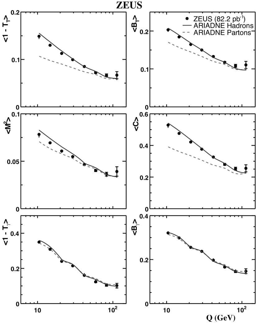
The mean values of the event-shape variables are compared with the Ariadne predictions in Fig. 1. In general, there is a good agreement between data and MC. However the MC tends to overestimate the shape variables at low , in particular . The Ariadne predictions at the parton level are also shown. The difference between the hadron and parton level demonstrates the contribution from the hadronisation process, as implemented in Ariadne. It should be noted that the parton level of Ariadne, defined by the parton shower model, does not have a rigorous meaning in pQCD [65] and should be taken as indicative only. The structure in the theoretical distributions results from the different -ranges associated with the bins, see Table 1.
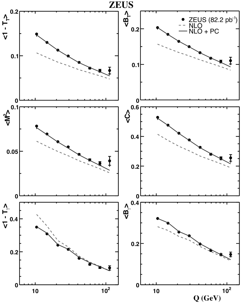
The mean values of the event-shape variables , , , , and as a function of were fitted, by varying and , to the sum of an NLO term obtained from DISASTER++, plus the power correction as given by Eq. (11). The data and fit results are shown in Fig. 2. For all variables the theory fits the data well. For , the best fit results in a negative power correction, whereas theory predicts a power correction equal to that found for .
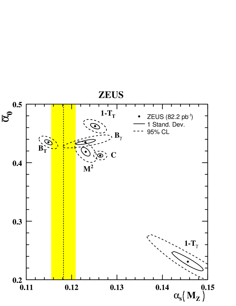
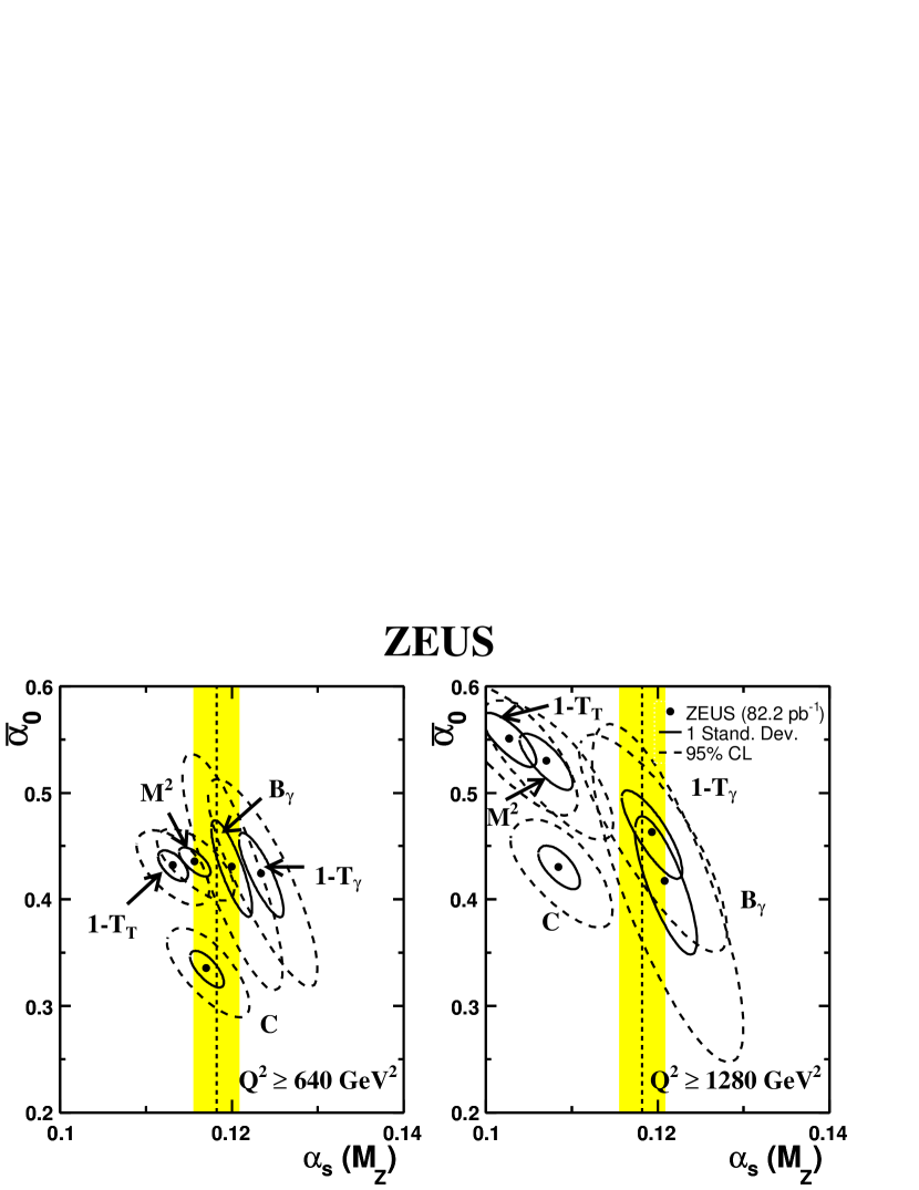
The extracted values are shown in Fig. 3 and in Tables 3 and 4. The contours on the plot represent one standard deviation errors, corresponding to about confidence level (CL), as well as the CL regions based on the fit errors as calculated using the Hessian method. The theoretical uncertainties are not shown but are given in the tables, since they result in a correlated shift to all fit results. The current world average, [66], is also shown.
The values are in good agreement with those previously published [13], but somewhat lower than those obtained by the H1 and experiments. The values of obtained from fits to , , and are roughly consistent with each other, but somewhat above the world average value. However, Tables 3 and 4 show that the theoretical uncertainties are substantial and strongly correlated between variables. Fits to and give values of which are inconsistent with the values obtained with the other variables, as already observed in the earlier ZEUS measurement.
For , the dominant uncertainty is that due to variation of the renormalisation scale. For , the variation in the Milan factor gives the largest uncertainty except in the case of . The PDF uncertainty was evaluated by replacing the CTEQ4 PDFs by the MRST99 set. With the exception of , the changes in the fitted are of the order of the Hessian fit error. For , the power correction becomes positive and the fitted values of () change to 0.1285(0.3541), values that are in closer agreement with the other variables. If the model were robust, the fitted values of would be independent of . However a dependence on is clearly evident in the tables. In view of these results, no attempt to extract combined values of from the mean event shapes was made.
10.2 Differential distributions
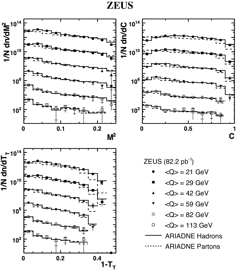
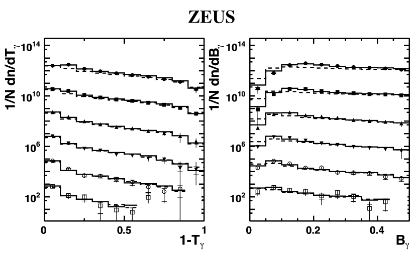
The differential distributions of the event-shape variables for are compared to the predictions of Ariadne in Figs. 4 and 5. For all variables, Ariadne describes the data well. The parton level of Ariadne is also shown. The difference between the hadron and parton levels can be taken as illustrative of the hadronisation correction.
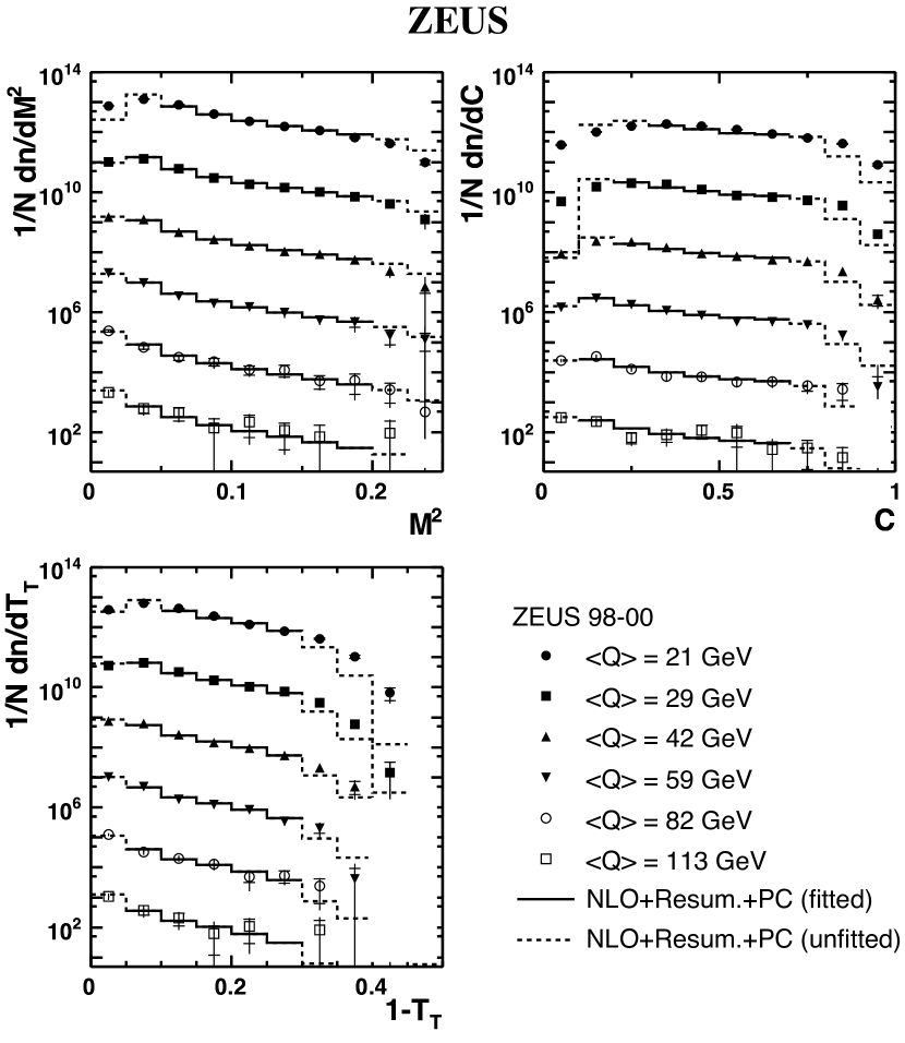
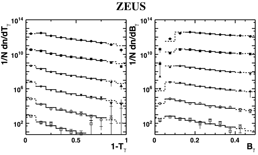
The differential distributions for , , , and , for which the theoretical predictions are available, have been fitted with NLL + NLO + PC calculations as shown in Figs. 6 and 7. The solid (dashed) bars show the bins that were used (unused) in the fit as described in Section 7.
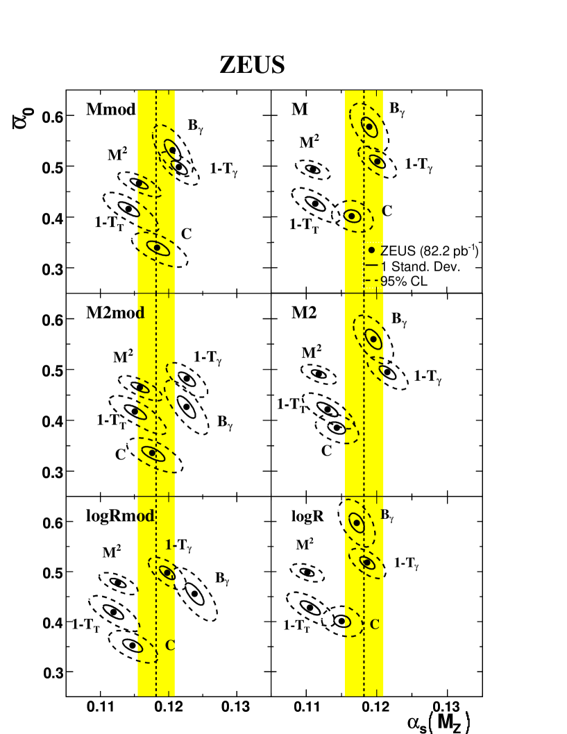
None of the three matching techniques discussed in Section 6.1 is strongly preferred theoretically. Although the modification terms should be used to ensure the correct behaviour of the cross section, all options included in DISRESUM have been used. The results of fits using six different matching options are shown in Fig. 8 and Tables 5 and 6. The of the fits does not depend significantly on the form of matching used. The M2mod matching has been chosen for this analysis in view of the minimal dispersion of and for this type of matching. Tables 5 and 6 show that the M2mod and Mmod matching techniques give fitted and values that agree, in general, within the Hessian fit errors; an exception is , which shows a five standard deviation shift in when the matching is changed from M2mod to Mmod. The logRmod matching gives larger systematic changes in the fitted (), of the order of two (one) standard deviation. In all cases, the unmodified matching schemes, which are theoretically disfavoured, result in larger shifts than the corresponding modified matching. It can be concluded that matching-scheme uncertainties are approximately twice the Hessian fit errors.
The results of the fit to the differential distributions using the M2mod matching scheme are summarised in Tables 7 and 8. The model gives a good description of the differential distributions for the global variables and over a substantial range of the shape variables; the of the fit is close to unity. For the non-global variables, , , , the fit is less good, with the lying in the range two to four. The fitted values are consistent with the world average. With the exception of , the values are consistent with those obtained from the mean values. Figure 9 shows that, for the global variables, the fitted values of and are consistent with being independent of the range. The non-global variables show a larger sensitivity to the range, possibly reflecting the poorer of the fits.
Tables 7 and 8 also give the theoretical uncertainties in the fitted values. For , the dominant theoretical uncertainties result from the renormalisation scale and the logarithmic rescale factor. The power factors in the modification terms also give rise to significant uncertainties for all variables except . In contrast to the results found for the mean values, changes in the Milan factor and have no significant influence on the fitted . In general, all systematic uncertainties, with exception of the check on PDFs, for are large compared to the fit errors and comparable in size to those of the mean fits.
An estimate of the influence of the fit range is given in the two final lines of Tables 7 and 8. This estimate was obtained by changing the fit range by half a bin at low values of the shape variable, where the influence of the NLL terms is greatest. For , the effect of the change is a few percent for and . In contrast, the fit values for the non-global variables are significantly dependent on the fit range. A comparison with the differential distributions measured by H1 shows reasonable agreement with this analysis. However, it should be noted that the two analyses differ in the kinematic range of the fits as well as in many details of the fits. The value of , given by H1, agrees with the interval, approximately 0.40.5, obtained in this analysis.
As in the case of the mean values, the fitted values of for the differential distributions are inconsistent with one another, with the non-global variables, , and , yielding a lower than the global variables and , irrespective of the matching scheme used. The uncertainties due to the fit range and theoretical parameters preclude a meaningful determination of the average values for and from the fits to the differential distribution.
10.3 Measurement of and
As discussed in Section 2, the analyses of the variable and were made in the full phase space of the Breit frame, including both the current and target regions. In contrast to the variables discussed previously, the correction to is expected to fall as . Although the general form of the correction is known, the theoretical calculations are not yet available. Consequently, no fit has been made but the data have been compared to Ariadne and NLO predictions. The distribution of and the mean of as a function of are shown in Figs. 10a and 10b, respectively, together with the Ariadne predictions at the hadron and parton levels. The figures show that Ariadne describes the distribution for well, but overestimates the means at lower .
In Fig. 10c, the distributions are compared with the NLO distribution from DISENT calculated using . Except at the lowest value for high , the NLO predictions describe the data well. In Fig. 10d, the mean values of are plotted as a function of and compared with the NLO predictions. The agreement with the NLO predictions is good over the entire range of .
The variable measures the momentum out of the event plane defined by two jets and thus depends on at lowest order. The data are compared to Ariadne predictions at the parton and hadron level in Fig. 11. For the differential distribution, at the parton level, Ariadne agrees well with the tail of the distribution but peaks at a lower value than the data. The hadron-level prediction, on the other hand, describes the data well everywhere, indicating the importance of hadronisation corrections to this variable. The mean value of agrees well with the expectation from Ariadne at the hadron level. In contrast, the parton-level predictions lie below the data, with a difference that decreases with , again indicating the importance of hadronisation effects.
11 Summary
Measurements have been made of mean values and differential distributions of the event-shape variables thrust , broadening , normalised jet mass , -parameter, and using the ZEUS detector at HERA. The variables and were determined relative to both the virtual photon axis and the thrust axis. The events were analysed in the Breit frame for the kinematic range , and . The data are well described by the Ariadne Monte Carlo model.
The dependence of the mean event shapes , , and , have been fitted to NLO calculations from perturbative QCD using the DISASTER++ program together with the Dokshitzer-Webber non-perturbative power corrections, with the strong coupling and the effective non-perturbative coupling as free parameters.
Consistent values of are obtained for the shape variables , , and , with values that agree to within . For , the value agrees with other variables, whereas does not. The variable gives and values that are inconsistent with the other variables and, in contrast to the other variables, that are sensitive to the parton density used in DISASTER++. For all variables, the renormalisation uncertainties, the dominant theoretical uncertainty, are three to ten times larger than the experimental uncertainties. Also the parameter used in the power corrections gives large uncertainties. These may be indications for the need for higher orders in the power corrections.
The program DISRESUM together with NLO calculations from DISPATCH has been used to fit the differential distributions for the event-shape variables , , , and for . A reasonable description is obtained for all variables. The modified matching schemes give fitted values of that are consistent with the world average. With the exception of , the values of are consistent with those found from the mean values and lie within the range 0.40.5.
Comparison between the and from the fits to different variables show, however, that the results are not consistent within the experimental uncertainties. The renormalisation uncertainties are still large. There is a considerable sensitivity to small changes in the kinematic range of fits, indicating problems in the theoretical description of the data. Also the choice of matching scheme produces variations of the order of the experimental uncertainties.
The power corrections for the variables and are not yet available. For , the data are well described by NLO calculations. The variable is well described by Ariadne predictions at the hadron level. A comparison of with parton and hadron level predictions of Ariadne indicates the need for substantial hadronisation corrections.
In summary, the power-correction method provides a reasonable description of the data for all event-shape variables studied. Nevertheless, the lack of consistency of the and determinations obtained in deep inelastic scattering, for the mean values in particular, suggests the importance of higher-order processes that are not yet included in the model.
Acknowledgements
It is a pleasure to thank the DESY Directorate for their strong support and encouragement. The remarkable achievements of the HERA machine group were essential for the successful completion of this work and are greatly appreciated. The design, construction and installation of the ZEUS detector has been made possible by the efforts of many people who are not listed as authors. We are indebted to M. Dasgupta, G. Salam, M. Seymour, G. Marchesini, G. Zanderighi and A. Banfi for many invaluable discussions.
10
References
- [1] B.R. Webber, Phys. Lett. B 339, 148 (1994)
- [2] Yu.L. Dokshitzer and B.R. Webber, Phys. Lett. B 352, 451 (1995)
- [3] G.P. Korchemsky and G. Sterman, Nucl. Phys. B 437, 415 (1995)
- [4] R. Akhoury and V.I. Zakharov, Phys. Lett. B 357, 646 (1995)
- [5] M. Beneke and V.M. Braun, Nucl. Phys. B 454, 253 (1995)
- [6] P.A. Movilla Fernández et al., Eur. Phys. J. C 22, 1 (2001) (and references therein)
- [7] Yu.L. Dokshitzer and B.R. Webber, Phys. Lett. B 404, 321 (1997)
- [8] Yu.L. Dokshitzer et al., Nucl. Phys. B 511, 396 (1998)
- [9] Erratum-ibid., Nucl. Phys. B 593, 729 (2001)
- [10] Yu.L. Dokshitzer, G. Marchesini and G.P. Salam, Eur. Phys. J. direct C 1, 3 (1999)
- [11] H1 Coll., C. Adloff et al., Eur. Phys. J. C 14, 255 (2000)
- [12] H1 Coll., A. Aktas et al., Eur. Phys. J. C 46, 343 (2006)
- [13] ZEUS Coll., S. Chekanov et al., Eur. Phys. J. C 27, 531 (2003)
- [14] R.P. Feynman, Photon-Hadron Interactions. Benjamin, New York, 1972
- [15] K.H. Streng, T.F. Walsh and P.M. Zerwas, Z. Phys. C 2, 237 (1979)
- [16] V. Antonelli, M. Dasgupta and G.P. Salam, JHEP 0002, 001 (2000)
- [17] S. Catani et al., Nucl. Phys. B 406, 187 (1993)
- [18] A. Banfi et al., JHEP 0111, 66 (2001)
- [19] ZEUS Coll., M. Derrick et al., Phys. Lett. B 293, 465 (1992)
- [20] ZEUS Coll., U. Holm (ed.), The ZEUS Detector. Status Report (unpublished), DESY (1993), available on http://www-zeus.desy.de/bluebook/bluebook.html
- [21] N. Harnew et al., Nucl. Inst. Meth. A 279, 290 (1989)
- [22] B. Foster et al., Nucl. Phys. Proc. Suppl. B 32, 181 (1993)
- [23] B. Foster et al., Nucl. Inst. Meth. A 338, 254 (1994)
- [24] M. Derrick et al., Nucl. Inst. Meth. A 309, 77 (1991)
- [25] A. Andresen et al., Nucl. Inst. Meth. A 309, 101 (1991)
- [26] A. Caldwell et al., Nucl. Inst. Meth. A 321, 356 (1992)
- [27] A. Bernstein et al., Nucl. Inst. Meth. A 336, 23 (1993)
- [28] J. Andruszków et al., Preprint DESY-92-066, DESY, 1992
- [29] ZEUS Coll., M. Derrick et al., Z. Phys. C 63, 391 (1994)
- [30] J. Andruszków et al., Acta Phys. Pol. B 32, 2025 (2001)
- [31] W.H. Smith, K. Tokushuku and L.W. Wiggers, Proceedings of the Computing in High Energy Physics (CHEP 92), C. Verkerk and W. Wojcik (eds.), p. 222. Geneva, Switzerland (1992). Also in preprint DESY 92-150B
- [32] ZEUS Coll., J. Breitweg et al., Eur. Phys. J. C 11, 427 (1999)
- [33] S. Bentvelsen, J. Engelen and P. Kooijman, Proc. Workshop on Physics at HERA, W. Buchmüller and G. Ingelman (eds.), Vol. 1, p. 23. Hamburg, Germany, DESY (1992)
- [34] F. Jacquet and A. Blondel, Proceedings of the Study for an Facility for Europe, U. Amaldi (ed.), p. 391. Hamburg, Germany (1979). Also in preprint DESY 79/48
- [35] G.M. Briskin, Ph.D. Thesis, Tel Aviv University, 1998. DESY-THESIS-1998-036
- [36] S.D. Ellis and D.E. Soper, Phys. Rev. D 48, 3160 (1993)
- [37] R. Brun et al., geant3, Technical Report CERN-DD/EE/84-1, CERN, 1987
- [38] K. Charchula, G.A. Schuler and H. Spiesberger, Comp. Phys. Comm. 81, 381 (1994)
- [39] G. Ingelman, A. Edin and J. Rathsman, Comp. Phys. Comm. 101, 108 (1997)
- [40] A. Kwiatkowski, H. Spiesberger and H.-J. Möhring, Comp. Phys. Comm. 69, 155 (1992)
- [41] L. Lönnblad, Comp. Phys. Comm. 71, 15 (1992)
- [42] B. Andersson et al., Phys. Rep. 97, 31 (1983)
- [43] M. Bengtsson and T. Sjöstrand, Comp. Phys. Comm. 46, 43 (1987)
- [44] T. Sjöstrand, Comp. Phys. Comm. 82, 74 (1994)
- [45] G. Marchesini et al., Comp. Phys. Comm. 67, 465 (1992)
- [46] G. Marchesini and B.R. Webber, Nucl. Phys. B 310, 461 (1988)
- [47] H.L. Lai et al., Phys. Rev. D 55, 1280 (1997)
- [48] D. Graudenz, Preprint hep-ph/9710244, 1997
- [49] S. Catani and M.H. Seymour, Nucl. Phys. B 485, 291 (1997)
- [50] M. Dasgupta and G.P. Salam, JHEP 0208, 032 (2002)
- [51] A.D. Martin et al., Eur. Phys. J. C 14, 133 (2000)
- [52] M. Dasgupta and G.P. Salam, Eur. Phys. J. C 24, 213 (2002)
- [53] M. Dasgupta and G.P. Salam, Phys. Lett. B 512, 3223 (2001)
- [54] R.W.L. Jones et al., JHEP 0312, 007 (2003)
- [55] M. Dasgupta and B.R. Webber, Eur. Phys. J. C 1, 539 (1998)
- [56] DELPHI Coll., P. Abreu et al., Z. Phys. C 73, 229 (1997)
- [57] DELPHI Coll., P. Abreu et al., Phys. Lett. B 456 (1999)
- [58] P.A. Movilla Fernández et al.and the JADE Coll., Eur. Phys. J. C 1, 461 (1998)
- [59] JADE Coll., O. Biebel et al., Phys. Lett. B 459, 326 (1999)
- [60] Yu.L. Dokshitzer et al., JHEP 9805, 3 (1998)
- [61] S. Hanlon, Ph.D. Thesis, University of Glasgow, 2004 (Unpublished)
- [62] A. Everett, Ph.D. Thesis, University of Wisconsin-Madison, 2006 (Unpublished)
- [63] D. Stump et al., Phys. Rev. D 65, 014012 (2002)
- [64] M. Botje, J. Phys. G 28, 779 (2002)
- [65] B.R. Webber, Nucl. Phys. Proc. Suppl. 71, 66 (1999)
- [66] S. Bethke, Nucl. Phys. Proc. Suppl. 135, 345 (2004)
| Bin | ) | |
|---|---|---|
| 1 | 80 160 | 0.0024 0.010 |
| 2 | 160 320 | 0.0024 0.010 |
| 3 | 320 640 | 0.01 0.05 |
| 4 | 640 1280 | 0.01 0.05 |
| 5 | 1280 2560 | 0.025 0.150 |
| 6 | 2560 5120 | 0.05 0.25 |
| 7 | 5120 10240 | 0.06 0.40 |
| 8 | 10240 20480 | 0.10 0.60 |
| ) | |||||
|---|---|---|---|---|---|
| Variable | ||||||
|---|---|---|---|---|---|---|
| Fit error | ||||||
| correlation | ||||||
| E-scheme | ||||||
| Variable | ||||||
|---|---|---|---|---|---|---|
| Fit error | ||||||
| E-scheme | ||||||
| Variable | |||||
|---|---|---|---|---|---|
| Fit error | |||||
| Variable | |||||
|---|---|---|---|---|---|
| Fit error | |||||
| Variable | |||||
|---|---|---|---|---|---|
| Fit error | |||||
| correlation | |||||
| E-scheme | |||||
| -0.5 Bins | |||||
| +0.5 Bins |
| Variable | |||||
|---|---|---|---|---|---|
| Fit error | |||||
| E-scheme | |||||
| -0.5 Bins | |||||
| +0.5 Bins |