A Study of the $D_{sJ}^{*}(2317)^{+}$ and $D_{sJ}(2460)^{+}$ Mesons in
Inclusive $c\overline{c}$ Production near $\sqrt{s}=10.6$ $\mathrm{\,Ge\kern-1.00006ptV}$

Abstract

A study of the $D_{sJ}^{*}(2317)^{+}$ and $D_{sJ}(2460)^{+}$ mesons in inclusive $c\bar{c}$ production is presented using 232 ${\rm fb}^{-1}$ of data collected by the BABAR  experiment near $\sqrt{s}=10.6$ $\mathrm{\,Ge\kern-1.00006ptV}$. Final states consisting of a $D^{+}_{s}$ meson along with one or more $\pi^{0}$, $\pi^{\pm}$, or $\gamma$ particles are considered. Estimates of the mass and limits on the width are provided for both mesons and for the $D_{s1}(2536)^{+}$ meson. A search is also performed for neutral and doubly-charged partners of the $D_{sJ}^{*}(2317)^{+}$ meson.

I Introduction

The $D_{sJ}^{*}(2317)^{+}$ meson, discovered by this collaboration Aubert et al. (2003) and confirmed by others Besson et al. (2003); Abe et al. (2004), does not conform to conventional models of $c\bar{s}$ meson spectroscopy. Included with this discovery were suggestions of a second state, the $D_{sJ}(2460)^{+}$ meson. This meson, observed by CLEO Besson et al. (2003) and confirmed by this collaboration Aubert et al. (2004a) and BELLE Abe et al. (2004), has a mass that is also lower than expectations Godfrey and Isgur (1985); Godfrey and Kokoski (1991); Isgur and Wise (1991); Di Pierro and Eichten (2001). Because the masses of these two states are so unusual there has been speculation Barnes et al. (2003); Lipkin (2004) that both possess an exotic, four-quark component. The possibility that the $D_{sJ}^{*}(2317)^{+}$ and $D_{sJ}(2460)^{+}$ are exotic has attracted considerable experimental and theoretical interest and has focused renewed attention on the subject of charmed-meson spectroscopy in general.

Presented in this paper is an updated analysis of these two states using $232$ ${\rm fb}^{-1}$ of $e^{+}e^{-}\to c\overline{c}$ data collected by the BABAR experiment. From this analysis new estimates of the $D_{sJ}^{*}(2317)^{+}$ and $D_{sJ}(2460)^{+}$ masses, limits on their intrinsic widths, calculations on their production cross sections, and the branching ratios of $D_{sJ}(2460)^{+}$ decays to $D^{+}_{s}\gamma$ and $D^{+}_{s}\pi^{+}\pi^{-}$ with respect to its decay to $D^{+}_{s}\pi^{0}\gamma$ are presented.

These measurements are performed by fitting the invariant mass spectra of combinations cpf of $D^{+}_{s}\pi^{0}$, $D^{+}_{s}\gamma$, $D^{+}_{s}\pi^{0}\gamma$, $D^{+}_{s}\pi^{0}\pi^{0}$, $D^{+}_{s}\gamma\gamma$, and $D^{+}_{s}\pi^{+}\pi^{-}$ particles. Combinations of $D^{+}_{s}\pi^{+}$ and $D^{+}_{s}\pi^{-}$ are also studied to search for new states. The mass spectrum of each final-state combination is studied in detail. In particular, features in the spectra that arise from reflections of other $c\bar{s}$ meson decays are individually identified and modeled. The analysis of the $D^{+}_{s}\pi^{0}\gamma$ final state includes an explicit search for the two most likely sub-resonant decay channels for $D_{sJ}(2460)^{+}$ meson decay.

This paper is organized as follows. First, the current status of the $D_{sJ}^{*}(2317)^{+}$ and $D_{sJ}(2460)^{+}$ mesons is reviewed. The reconstruction of $D^{+}_{s}$, $\pi^{0}$, $\gamma$, and $\pi^{\pm}$ candidates is then described, including an estimate of $D^{+}_{s}$ yield in terms of the $D^{+}_{s}\to\phi\pi^{+}$ branching fraction. Each combination of final-state particle species is then discussed individually. The paper finishes with a summary of results and conclusions.

II Review of the $D_{sJ}^{*}(2317)^{+}$ and $D_{sJ}(2460)^{+}$

Much of the theoretical work on the $c\bar{s}$ system has been performed in the limit of heavy $c$ quark mass using potential models Godfrey and Isgur (1985); Godfrey and Kokoski (1991); Isgur and Wise (1991); Di Pierro and Eichten (2001) that treat the $c\bar{s}$ system much like a hydrogen atom. Prior to the discovery of the $D_{sJ}^{*}(2317)^{+}$ meson, such models were successful at explaining the masses of all known $D$ and $D_{s}$ states and even predicting, to good accuracy, the masses of many $D$ mesons (including the $D_{s1}(2536)^{+}$ and $D_{s2}(2573)^{+}$) before they were observed (see Fig. 1). Several of the predicted $D_{s}$ states were not confirmed experimentally, notably the lowest mass $J^{P}=0^{+}$ state (at around 2.48 ${\mathrm{\,Ge\kern-1.00006ptV\!/}c^{2}}$) and the second lowest mass $J^{P}=1^{+}$ state (at around 2.58 ${\mathrm{\,Ge\kern-1.00006ptV\!/}c^{2}}$). Since the predicted widths of these two states were large, they would be hard to observe, and thus the lack of experimental evidence was not a concern.

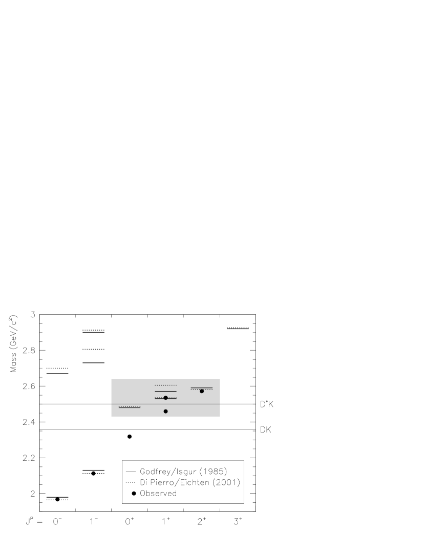
Figure 1: The $c\bar{s}$ meson spectrum, as predicted by Godfrey and Isgur Godfrey and Isgur (1985) (solid lines) and Di Pierro and Eichten Di Pierro and Eichten (2001) (dashed lines) and as observed by experiment (points). The $DK$ and $D^{*}K$ mass thresholds are indicated by the horizontal lines spanning the width of the plot.

The $D_{sJ}^{*}(2317)^{+}$ meson has been observed in the decay $D_{sJ}^{*}(2317)^{+}\to D^{+}_{s}\pi^{0}$ Aubert et al. (2003); Besson et al. (2003); Abe et al. (2004); Krokovny et al. (2003); Aubert et al. (2004b). The mass is measured to be around $2.32$ ${\mathrm{\,Ge\kern-1.00006ptV\!/}c^{2}}$, which is below the $DK$ threshold. Thus, this particle is forced to decay either electromagnetically, of which there is no experimental evidence, or through the observed isospin-violating $D^{+}_{s}\pi^{0}$ strong decay. The intrinsic width is small enough that only upper limits have been measured (the best limit previous to this paper being $\Gamma<4.6$ $\mathrm{\,Me\kern-1.00006ptV}$  at 95% CL as established by BELLE Abe et al. (2004)). If the $D_{sJ}^{*}(2317)^{+}$ is the missing $0^{+}$ $c\bar{s}$ meson state, the narrow width could be explained by the lack of an isospin-conserving strong decay channel. The low mass (160 ${\mathrm{\,Me\kern-1.00006ptV\!/}c^{2}}$  below expectations) is more surprising and has led to the speculation that the $D_{sJ}^{*}(2317)^{+}$ does not belong to the $D^{+}_{s}$ meson family at all but is instead some type of exotic particle, such as a four-quark state Barnes et al. (2003).

The $D_{sJ}(2460)^{+}$ meson has been observed decaying to $D^{+}_{s}\pi^{0}\gamma$ Besson et al. (2003); Aubert et al. (2004a); Abe et al. (2004); Krokovny et al. (2003); Aubert et al. (2004b), $D^{+}_{s}\pi^{+}\pi^{-}$ Abe et al. (2004), and $D^{+}_{s}\gamma$ Abe et al. (2004); Krokovny et al. (2003); Aubert et al. (2004b). The intrinsic width is small enough that only upper limits have been measured (the best limit previous to this paper being $\Gamma<5.5$ $\mathrm{\,Me\kern-1.00006ptV}$  at 95% CL as established by BELLE Abe et al. (2004)). The $D^{+}_{s}\gamma$ decay implies a spin of at least one, and so it is natural to assume that the $D_{sJ}(2460)^{+}$ is the missing $1^{+}$ $c\bar{s}$ meson state. Like the $D_{sJ}^{*}(2317)^{+}$, the $D_{sJ}(2460)^{+}$ is substantially lower in mass than predicted for the normal $c\bar{s}$ meson. This suggests that a similar mechanism is deflating the masses of both mesons, or that both the states belong to the same family of exotic particles.

The spin-parity of the $D_{sJ}^{*}(2317)^{+}$ and $D_{sJ}(2460)^{+}$ mesons has not been firmly established. The decay mode of the $D_{sJ}^{*}(2317)^{+}$ alone implies a spin-parity assignment from the natural $J^{P}$ series $\{0^{+},1^{-},2^{+},\dots\}$, assuming parity conservation. Because of the low mass, the assignment $J^{P}=0^{+}$ seems most reasonable, although experimental data have not ruled out higher spin. It is not clear whether electromagnetic decays such as $D_{s}^{*}(2112)^{+}\gamma$ can compete with the strong decay to $D^{+}_{s}\pi^{0}$, even with isospin violation. Thus, the absence of experimental evidence for radiative decays such as $D_{sJ}^{*}(2317)^{+}\to D_{s}^{*}(2112)^{+}\gamma$ is not conclusive.

Experimental evidence for the spin-parity of the $D_{sJ}(2460)^{+}$ meson is somewhat stronger. The observation of the decay to $D^{+}_{s}\gamma$ alone rules out $J=0$. Decay distribution studies in $B\to D_{sJ}(2460)^{+}D_{s}^{(*)-}$ Krokovny et al. (2003); Aubert et al. (2004b) favor the assignment $J=1$. Decays to either $D^{+}_{s}\pi^{0}$, $D^{0}K^{+}$, or $D^{+}K^{0}$ would be favored if they were allowed. Since these decay channels are not observed, this suggests, when combined with the other observations, the assignment $J^{P}=1^{+}$. In this case, the decay to $D_{sJ}^{*}(2317)^{+}\gamma$ is allowed, but it may be small in comparison to the $D^{+}_{s}\gamma$ decay mode.

Table 1 lists various possible decay channels for the $D_{sJ}^{*}(2317)^{+}$ and $D_{sJ}(2460)^{+}$ mesons. Several of these decays are forbidden assuming the spin-parity assignments discussed above.

Table 1: A list of various decay channels and whether they have been seen, are allowed, or are forbidden in the decay of the $D_{sJ}^{*}(2317)^{+}$ and $D_{sJ}(2460)^{+}$ mesons. The predictions assume a spin-parity assignment of $J^{P}=0^{+}$ and $1^{+}$, respectively.

Decay Channel		$D_{sJ}^{*}(2317)^{+}$	$D_{sJ}(2460)^{+}$
$D^{+}_{s}\pi^{0}$		Seen	Forbidden
$D^{+}_{s}\gamma$		Forbidden	Seen
$D^{+}_{s}\pi^{0}\gamma$ (a)		Allowed	Allowed
	$D_{s}^{*}(2112)^{+}\pi^{0}$	Forbidden	Seen
	$D_{sJ}^{*}(2317)^{+}\gamma$	—	Allowed
$D^{+}_{s}\pi^{0}\pi^{0}$		Forbidden	Allowed
$D^{+}_{s}\gamma\gamma$ (a)		Allowed	Allowed
	$D_{s}^{*}(2112)^{+}\gamma$	Allowed	Allowed
$D^{+}_{s}\pi^{+}\pi^{-}$		Forbidden	Seen

(a) Non-resonant only

III The BABAR  Detector and Dataset

The data used in this analysis were recorded with the BABAR detector at the PEP-II asymmetric-energy storage rings and correspond to an integrated luminosity of 232 ${\rm fb}^{-1}$ collected on or just below the $\Upsilon(4S)$ resonance.

A detailed description of the BABAR detector is presented elsewhere Aubert et al. (2002). Charged particles are detected with a five-layer, double-sided silicon vertex tracker (SVT) and a 40-layer drift chamber (DCH) using a helium-isobutane gas mixture, placed in a 1.5-T solenoidal field produced by a superconducting magnet. The charged-particle momentum resolution is approximately $(\delta p_{T}/p_{T})^{2}=(0.0013\,p_{T})^{2}+(0.0045)^{2}$, where $p_{T}$ is the transverse momentum in ${\mathrm{\,Ge\kern-1.00006ptV\!/}c}$. The SVT, with a typical single-hit resolution of 10${\,\mu\rm m}$, measures the impact parameters of charged-particle tracks in both the plane transverse to the beam direction and along the beam. Charged-particle types are identified from the ionization energy loss ($\mathrm{d}E/\mathrm{d}x$) measured in the DCH and SVT, and from the Cherenkov radiation detected in a ring-imaging Cherenkov device (DIRC). Photons are detected by a CsI(Tl) electromagnetic calorimeter (EMC) with an energy resolution $\sigma(E)/E=0.023\cdot(E/\mathrm{\,Ge\kern-1.00006ptV})^{-1/4}\oplus 0.019$. The return yoke of the superconducting coil is instrumented with resistive plate chambers (IFR) for the identification of muons and the detection of neutral hadrons.

IV Candidate Reconstruction

The goal of this analysis is to study the possible decay of the $D_{sJ}^{*}(2317)^{+}$ and $D_{sJ}(2460)^{+}$ mesons into the final states listed in Table 1. These decay channels consist of one $D^{+}_{s}$ meson combined with up to two additional particles selected from $\pi^{0}$, $\pi^{\pm}$, and $\gamma$. The first step in this analysis is to identify $D^{+}_{s}$ mesons in the BABAR data. For each resulting $D^{+}_{s}$ candidate a search is performed for associated $\pi^{0}$, $\gamma$, and $\pi^{\pm}$ particles. Signals from $D_{sJ}^{*}(2317)^{+}$ and $D_{sJ}(2460)^{+}$ decay are isolated using the invariant mass of the desired combination of particle species.

The $D^{+}_{s}\to K^{+}K^{-}\pi^{+}$ decay mode is used to select a high-statistics sample of $D^{+}_{s}$ meson candidates. Each $K^{\pm}$ and $\pi^{\pm}$ candidate is separated from other charged particle species by a likelihood-based particle identification algorithm based on the Cherenkov-photon information from the DIRC together with $\mathrm{d}E/\mathrm{d}x$ measurements from the SVT and DCH. A geometrical fit to a common vertex is applied to each $K^{+}K^{-}\pi^{+}$ combination. An acceptable $K^{+}K^{-}\pi^{+}$ candidate must have a fit probability greater than 0.1% and a trajectory consistent with originating from the $e^{+}e^{-}$ luminous region. To reduce combinatorial background, each $K^{+}K^{-}\pi^{+}$ candidate must have a momentum $p^{*}$ in the $e^{+}e^{-}$ center-of-mass frame greater than 2.2 ${\mathrm{\,Ge\kern-1.00006ptV\!/}c^{2}}$, a requirement that also removes nearly all contributions from $B$-meson decay. Background from $D^{0}\to K^{+}K^{-}$, which is evident from the corresponding $K^{+}K^{-}$ mass distribution, is removed by requiring that the $K^{+}K^{-}$ mass be less than 1.84 ${\mathrm{\,Ge\kern-1.00006ptV\!/}c^{2}}$.

The upper histogram in Fig. 2(a) shows the $K^{+}K^{-}\pi^{+}$ mass distribution for all candidates. A clear $D^{+}_{s}$ signal is seen. To reduce the background further, only those candidates with $K^{+}K^{-}$ mass within 10 ${\mathrm{\,Me\kern-1.00006ptV\!/}c^{2}}$ of the $\phi(1020)$ mass or with $K^{-}\pi^{+}$ mass within 50 ${\mathrm{\,Me\kern-1.00006ptV\!/}c^{2}}$ of the $\kern 1.99997pt\overline{\kern-1.99997ptK}{}^{*}(892)$ mass are retained; these densely populated regions in the $D_{s}^{+}$ Dalitz plot do not overlap (see Fig. 3). The decay products of the vector particles $\phi(1020)$ and $\kern 1.99997pt\overline{\kern-1.99997ptK}{}^{*}(892)$ exhibit the expected $\cos^{2}\theta_{h}$ behavior required by conservation of angular momentum, where $\theta_{h}$ is the helicity angle. The signal-to-background ratio is further improved by requiring $|\cos\theta_{h}|>0.5$. The lower histogram of Fig. 2(a) shows the net effect of these additional selection criteria. The $D_{s}^{+}$ signal ($1.954<m(K^{+}K^{-}\pi^{+})<1.981$ ${\mathrm{\,Ge\kern-1.00006ptV\!/}c^{2}}$) and sideband ($1.912<m(K^{+}K^{-}\pi^{+})<1.934~{}{\mathrm{\,Ge\kern-1.00006ptV\!/}c^{2}}$ and $1.998<m(K^{+}K^{-}\pi^{+})<2.020$ ${\mathrm{\,Ge\kern-1.00006ptV\!/}c^{2}}$) regions are shaded. This distribution can be reasonably modeled in a $\chi^{2}$ fit by the sum of two Gaussian distributions with a common mean (hereafter referred to as a double Gaussian) on top of a quadratic background. The result of this fit is a $D^{+}_{s}$ signal peak consisting of approximately 410 000 decays and a mass of $1967.8$ ${\mathrm{\,Me\kern-1.00006ptV\!/}c^{2}}$ with negligible statistical error.

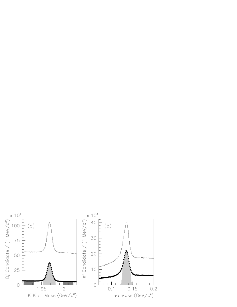
Figure 2: (a) The invariant mass spectrum of $D^{+}_{s}$ candidates before (top histogram) and after (bottom points) applying subresonant $\phi\pi^{+}$ and $\kern 1.99997pt\overline{\kern-1.99997ptK}{}^{*}K^{+}$ selection. The light (dark) areas indicate the signal (sideband) regions. (b) The invariant $\gamma\gamma$ mass of $\pi^{0}$ candidates before (top histogram) and after (bottom points) applying the $\pi^{0}$ veto described in the text. The light histogram indicates those candidates that pass the $\chi^{2}$ requirement. The curve in (a) is the $\chi^{2}$ fit described in the text.

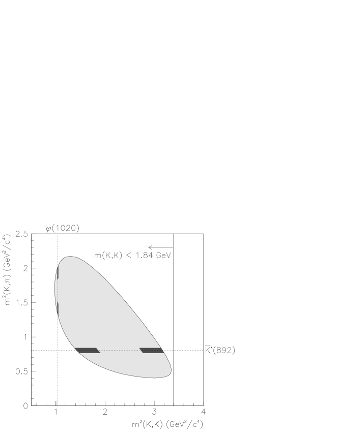
Figure 3: An illustration of the $D^{+}_{s}$ sub-resonant selection requirements. The light shaded area is the kinematic range for $D^{+}_{s}\to K^{+}K^{-}\pi^{+}$ decay. The vertical line with an arrow represents the selection requirement used to remove $D^{0}\to K^{+}K^{-}$ decay. The four dark regions indicate those portions of the $D^{+}_{s}$ phase space used for final candidate selection, corresponding to $D^{+}_{s}\to\phi\pi^{+}$ and $D^{+}_{s}\to\kern 1.99997pt\overline{\kern-1.99997ptK}{}^{*}K^{+}$ decay.

The approximate $p^{*}$ distribution for selected $D^{+}_{s}$ mesons can be obtained by simple sideband subtraction, assuming linear background behavior under the $D^{+}_{s}$. The result is shown in Fig. 4.

The final list of $D^{+}_{s}$ candidates are those that lie within the signal window. For each such candidate, the momentum vector is calculated from the simple addition of $K^{+}$, $K^{-}$, and $\pi^{+}$ momentum vectors. The energy is chosen to reproduce the PDG value for the $D^{+}_{s}$ mass ($1968.5\pm 0.5)$ ${\mathrm{\,Me\kern-1.00006ptV\!/}c^{2}}$ Eidelman et al. (2004).

Figure 4: The sideband subtracted $p^{*}$ spectrum for $D^{+}_{s}$ candidates after all selection requirements are met.

It is assumed that the $D_{sJ}^{*}(2317)^{+}$ and $D_{sJ}(2460)^{+}$ mesons have lifetimes that are too small to be resolved by the detector. Thus, the most likely point of $D_{sJ}^{*}(2317)^{+}$ and $D_{sJ}(2460)^{+}$ decay for each $D^{+}_{s}$ candidate is chosen to be the interaction point (IP), calculated from the intersection of the trajectory of the candidate and the $e^{+}e^{-}$ luminous region. To produce a list of $\pi^{\pm}$ particles that could arise from $D_{sJ}^{*}(2317)^{+}$ or $D_{sJ}(2460)^{+}$ decay, the trajectories of all $\pi^{\pm}$ candidates that are not daughters of the $D^{+}_{s}$ candidate are constrained to the IP using a geometric vertex fit. The approximate $p^{*}$ spectrum of these candidates associated with real $D^{+}_{s}$ mesons can be obtained by using simple $D^{+}_{s}$ sideband subtraction. The result is shown in Fig. 5(a).

Figure 5: The $D^{+}_{s}$-sideband subtracted $p^{*}$ spectrum for associated (a) $\pi^{\pm}$, (b) $\pi^{0}$, and (c) $\gamma$, after the selection requirements described in the text are fulfilled.

The selection of $\gamma$ and $\pi^{0}$ candidates is a two-step process. The first step is the selection of a fiducial list of $\gamma$ and $\pi^{0}$ candidates. The fiducial list of $\gamma$ candidates is constructed from energy clusters in the EMC with energies above 100 $\mathrm{\,Me\kern-1.00006ptV}$  and not associated with a charged track. The energy centroid in the EMC combined with the IP position is used to calculate the $\gamma$ momentum direction. Each fiducial $\pi^{0}$ candidate is constructed from a pair of $\gamma$ particles in the $\gamma$ fiducial list. This $\gamma$ pair is combined using a kinematic fit assuming a $\pi^{0}$ mass. The resulting $\pi^{0}$ momentum is required to be greater than 150 ${\mathrm{\,Me\kern-1.00006ptV\!/}c}$. The $\gamma\gamma$ invariant mass spectrum from this $\pi^{0}$ selection is shown in the top histogram of Fig. 2(b). To produce the final fiducial list of $\pi^{0}$ candidates, the $\chi^{2}$ probability of the kinematic fit is required to be greater than 2%.

The final list of $\gamma$ candidates consists of any $\gamma$ in the fiducial list that is not used in the construction of any $\pi^{0}$ in the $\pi^{0}$ fiducial list. The final list of $\pi^{0}$ candidates consists of any $\pi^{0}$ in the fiducial list that does not share a $\gamma$ with any other $\pi^{0}$ in the fiducial list. The $\gamma\gamma$ invariant mass distribution of the final list of $\pi^{0}$ candidates is shown in the bottom histograms of Fig. 2(b), both before and after applying the $\chi^{2}$ probability requirement. The approximate $p^{*}$ spectrum of the final list of $\gamma$ and $\pi^{0}$ candidates as determined using $D^{+}_{s}$ sideband subtraction is shown in Figs. 5(b) and 5(c).

V Monte Carlo Simulation

Monte Carlo (MC) simulation is used for the following purposes in this paper:

• To calculate signal efficiencies.

• To provide independent estimates of background levels.

• To characterize the reconstructed mass distribution of the signal.

• To predict the behavior of various specific types of backgrounds (commonly referred to as reflections) produced when the mass distribution from an established decay mode is distorted by the loss of one or more final-state particles or the addition of one or more unassociated particles.

Various sets of MC events were generated. For the purposes of understanding signal efficiencies, signal shapes, and reflections, individual MC sets of 500 000 decays were generated for each known decay mode of the $D_{sJ}^{*}(2317)^{+}$ and $D_{sJ}(2460)^{+}$ mesons. In addition, MC sets of 250 000 decays were produced for each hypothetical $D_{sJ}^{*}(2317)^{+}$ and $D_{sJ}(2460)^{+}$ decay as needed. Finally, a set of $e^{+}e^{-}\to c\bar{c}$ events, corresponding to an integrated luminosity of approximately 80 ${\rm fb}^{-1}$, was generated to study sources of combinatorial background.

Each MC set was processed by the same reconstruction and selection algorithms used for the data. Independent tests of the detector simulation have demonstrated an accurate reproduction of charged particle detection efficiency. The systematic uncertainty from these tests is estimated to be 1.3% for each charged track. Since the decay $D^{+}_{s}\to K^{+}K^{-}\pi^{+}$ involves three charged tracks, the systematic uncertainty in $D^{+}_{s}$ efficiency from the simulation alone is estimated to be 3.9%.

The simulation of $D^{+}_{s}\to K^{+}K^{-}\pi^{+}$ decay was designed to match approximately the known Dalitz structure. MC events were reweighted to match more precisely the relative $\phi\pi^{+}$ and $\kern 1.99997pt\overline{\kern-1.99997ptK}{}^{*}K^{+}$ yields observed in the data.

The simulation assumes a $D_{sJ}^{*}(2317)^{+}$ and $D_{sJ}(2460)^{+}$ intrinsic width of $\Gamma=0.1$ $\mathrm{\,Me\kern-1.00006ptV}$. All $D_{sJ}^{*}(2317)^{+}$ and $D_{sJ}(2460)^{+}$ final states are generated using phase space. The generated $p^{*}$ distribution of $D_{sJ}^{*}(2317)^{+}$ and $D_{sJ}(2460)^{+}$ mesons in the MC simulation was adjusted to roughly reproduce observations.

VI Absolute $D^{+}_{s}$ Yield

In order to calculate $D_{sJ}^{*}(2317)^{+}$ and $D_{sJ}(2460)^{+}$ production cross sections, it is necessary to provide an estimate of absolute $D^{+}_{s}$ selection efficiency. Since this analysis uses $D^{+}_{s}\to K^{+}K^{-}\pi^{+}$ decay, the approach is to normalize $D^{+}_{s}$ yield with respect to the $D^{+}_{s}\to\phi\pi^{+},\phi\to K^{+}K^{-}$ branching fraction, the world average of which is $1.8\pm 0.4$% Eidelman et al. (2004). To perform this normalization correctly, the following must be accounted for:

• The $\kern 1.99997pt\overline{\kern-1.99997ptK}{}^{*}K^{+}$ portion of the $D^{+}_{s}$ sample.

• Non-resonant $K^{+}K^{-}\pi^{+}$ background under the $\phi$ peak.

• The fraction of the $\phi$ signal that falls outside of the $K^{+}K^{-}$ mass selection and $\theta_{h}$ requirements.

The $\kern 1.99997pt\overline{\kern-1.99997ptK}{}^{*}K^{+}$ selection represents approximately 48% of the total $D^{+}_{s}$ sample. An inspection of the $p^{*}$ distribution of the $\phi\pi^{+}$ and $\kern 1.99997pt\overline{\kern-1.99997ptK}{}^{*}K^{+}$ subsamples indicates that this fraction is, to a good approximation, independent of $p^{*}$. Therefore, a constant factor is sufficient to account for the contribution from the $\kern 1.99997pt\overline{\kern-1.99997ptK}{}^{*}K^{+}$ portions of the $D^{+}_{s}$ sample.

Shown in Fig. 6 is the $D^{+}_{s}$-sideband subtracted $K^{+}K^{-}$ invariant mass spectrum for all $D^{+}_{s}$ candidates before applying the $\phi\pi^{+}$ and $\kern 1.99997pt\overline{\kern-1.99997ptK}{}^{*}K^{+}$ selection requirements. A prominent $\phi$ peak is observed. A binned $\chi^{2}$ fit to this spectrum is used to extract both the fraction of $\phi\pi^{+}$ decays that fall outside the $\phi$ selection window and the number of non-$\phi$ decays that leak inside. This fit is described below.

Figure 6: The $D^{+}_{s}$-sideband subtracted $K^{+}K^{-}$ invariant mass spectrum near the $\phi$ mass for the $D^{+}_{s}$ sample obtained before applying the $\phi\pi^{+}$ and $\kern 1.99997pt\overline{\kern-1.99997ptK}{}^{*}K^{+}$ selection requirements. The curve is the fit described in the text. The dashed line is the portion of the fit attributed to contributions from other than $\phi$ decay. The vertical lines indicate the $\phi$ mass selection window.

To model the signal portion of the $K^{+}K^{-}$ mass spectrum, the $\phi\to K^{+}K^{-}$ line shape $\sigma(m)$ can be reasonably well described (ignoring potential interference effects) by a relativistic Breit-Wigner function:

$$\sigma(m)=\frac{m\Gamma(m)}{\left(m^{2}-m^{2}_{0}\right)^{2}+m_{0}^{2}\Gamma_{\text{tot}}^{2}(m)}\;,$$ (1)

where $m_{0}=(1019.456\pm 0.020)$ ${\mathrm{\,Me\kern-1.00006ptV\!/}c^{2}}$  is the intrinsic $\phi$ mass Eidelman et al. (2004). The mass-dependent width $\Gamma(m)$ can be approximated by:

$$\Gamma(m)=0.493\Gamma_{0}\frac{m_{0}}{m}\left(\frac{q}{q_{0}}\right)^{3}\frac{1+q_{0}^{2}R^{2}}{1+q^{2}R^{2}}\;,$$ (2)

where $\Gamma_{0}=4.26$ $\mathrm{\,Me\kern-1.00006ptV}$  is the intrinsic width, 0.493 is the branching fraction for this decay mode, $R=3$ $\mathrm{\,Ge\kern-1.00006ptV}^{-1}$ is an effective $\phi$ radius (to control the tails), and $q$ ($q_{0}$) is the total three-momentum of the $K^{\pm}$ decay products in the $\phi$ center-of-mass frame assuming an effective $\phi$ mass of $m$ ($m_{0}$):

$$q=\sqrt{m^{2}/4-m_{K}^{2}}\quad\text{and}\quad q_{0}=\sqrt{m^{2}_{0}/4-m_{K}^{2}}\;.$$ (3)

A reasonable approximation of the total width includes the three dominant decay modes ($K^{+}K^{-}$, $K_{S}K_{L}$, $\pi^{+}\pi^{-}\pi^{0}$):

$$\Gamma_{\text{tot}}(m)=\Gamma(m)+\Gamma^{\prime}(m)+0.155\Gamma_{0}\;,$$ (4)

where $\Gamma^{\prime}(m)$ is calculated in the same manner as $\Gamma(m)$ but using the $K_{S}/K_{L}$ mass and branching fraction (0.337) and the width for the three-pion decay mode (which is well above threshold) is treated as a constant.

The fit function $P(m)$ used to describe the $K^{+}K^{-}$ mass spectrum of Fig. 6 is:

$$P(m)=S_{\phi}(m)+C(m)\;,$$ (5)

where $S_{\phi}(m)$ is the $\phi$ signal shape and $C(m)$ represents non-resonant contributions. The empirical form used for $C(m)$ is a four-parameter threshold function:

$$C(m) = \left\{\begin{array}[]{ll}0&m<a_{1}\\ C^{\prime}(m)&m\geq a_{1}\end{array}\right.$$ (8)

$$C^{\prime}(m) = \left(1+m-a_{1}\right)^{a_{2}}\left(1-\exp(-\left(m-a_{0})/a_{3}\right)\right)\;.$$

The form used for $S_{\phi}(m)$ is the Breit-Wigner function of Eq. 1 smeared by a Gaussian:

$$S_{\phi}(m)=\frac{N}{\delta\sqrt{2\pi}}\int\sigma(m^{\prime})\>e^{-\left(m-m^{\prime}\right)^{2}/2\delta^{2}}\>{\rm d}m^{\prime}\;,$$ (9)

where $N$ is an overall normalization. In the fit to this function, the value of $\Gamma_{0}$ is kept fixed to the PDG value but $m_{0}$ and $\delta$ are allowed to vary.

Despite its simplicity, the function of Eq. 5 describes the $K^{+}K^{-}$ spectrum quite well, as shown in Fig. 6. The value of $m_{0}$ produced by the fit is slightly lower [($-56\pm 6$) ${\mathrm{\,ke\kern-1.00006ptV\!/}c^{2}}$, statistical error only] than the PDG average Eidelman et al. (2004). To determine a correction factor for the $D^{+}_{s}$ yield, the total $\phi$ yield (calculated from the integral of the signal line shape determined by the fit up to a $K^{+}K^{-}$ mass of 1.1 ${\mathrm{\,Ge\kern-1.00006ptV\!/}c^{2}}$) can be compared to the total number of candidates which fall inside the $\phi$ mass window. The result is a correction factor of 1.09, with negligible statistical uncertainty.

To test the above calculation, the fit is repeated on a $D^{+}_{s}$ sample that includes the $|\cos\theta_{h}|>0.5$ requirement discussed earlier for the $\phi$. The change in $\phi$ integrated yield is consistent with a $\cos^{2}\theta_{h}$ distribution. The measured correction factor increases to 1.10. The difference between this value and $1.09$ is taken as a systematic uncertainty.

Other systematic checks performed include increasing the range in $K^{+}K^{-}$ mass of the $\phi$ line shape integration and changing the value of $R$ from 1 to 5 ${\mathrm{\,Ge\kern-1.00006ptV\!/}c^{2}}$. The total uncertainty in the 1.09 correction factor is found to be a 0.043 (3.9% relative), as calculated from a quadrature sum.

VII Candidate Selection Optimization

This paper explores the eight final-state combinations shown in Table 2, each involving a $D^{+}_{s}$ meson and up to two total of $\pi^{\pm}$, $\pi^{0}$, and/or $\gamma$ particles. For each combination it is necessary to distinguish possible signals from $D_{sJ}^{*}(2317)^{+}$ and $D_{sJ}(2460)^{+}$ decay from combinatorial background. The separation of signal and background is made more distinct if additional candidate selection requirements are imposed. This section discusses those additional requirements.

In four of the final-state combinations ($D^{+}_{s}\pi^{0}$, $D^{+}_{s}\pi^{0}\gamma$, $D^{+}_{s}\gamma$, and $D^{+}_{s}\pi^{+}\pi^{-}$) a signal is expected. An estimate of signal significance is calculated in these cases based on expected signal and background rates, the former calculated from previously published branching ratio measurements combined with the appropriate MC sample. For the remainder of the final states, an estimate of signal sensitivity is calculated for the hypothetical $D_{sJ}^{*}(2317)^{+}$ and $D_{sJ}(2460)^{+}$ meson decay. This sensitivity calculation is based on signal efficiency, determined using MC samples, and expected background levels.

To avoid potential biases, both the signal significance and sensitivity estimates are calculated solely using MC samples.

The following selection requirements are adjusted in order to produce optimal values of signal significance and sensitivity:

• A minimum total center-of-mass momentum $p^{*}$.

• A minimum energy (for $\gamma$) and/or momentum calculated in the laboratory (for $\pi^{0}$) or center-of-mass (for $\pi^{\pm}$) frame of reference.

For the minimum $p^{*}$, it is important to choose the same value for all final-state combinations in order to minimize systematic uncertainties in the branching ratios. A minimum value of $p^{*}>3.2$ ${\mathrm{\,Ge\kern-1.00006ptV\!/}c}$ is chosen as a reasonable compromise. Values for the remaining selection requirements are chosen separately for each final-state combination. The results are listed in Table 2.

The MC samples can be used to estimate the approximate efficiency for detecting a signal with a $p^{*}$ of at least 3.2 ${\mathrm{\,Ge\kern-1.00006ptV\!/}c}$  after applying the above selection requirements. The resulting efficiencies vary between 0.4% and 13% (see Table 2).

Table 2: Selection requirements for the final states studied in this paper, the resulting number of events, and the approximate efficiency for a $D_{sJ}(2460)^{+}$ signal. The selection requirements are specified either in the laboratory (Lab) or center-of-mass (CMS) coordinate systems.

	Minimum Requirements
	$\gamma$ Energy	$\pi^{0}$ Mom.	$\pi^{\pm}$ Mom.
	Lab	Lab	CMS	Sample	Effic.
Final State	($\mathrm{\,Me\kern-1.00006ptV}$)	(${\mathrm{\,Me\kern-1.00006ptV\!/}c}$)	(${\mathrm{\,Me\kern-1.00006ptV\!/}c}$)	Size	(%)
$D^{+}_{s}\pi^{0}$	—	350	—	87 320	6.4
$D^{+}_{s}\gamma$	500	—	—	133 398	12
$D^{+}_{s}\pi^{0}\gamma$	135	400	—	170 341	2.4
$D^{+}_{s}\pi^{0}\pi^{0}$	—	250	—	17 437	0.4
$D^{+}_{s}\gamma\gamma$	170	—	—	575 765	7.9
$D^{+}_{s}\pi^{+}$	—	—	300	143 149	13
$D^{+}_{s}\pi^{-}$	—	—	300	219 466	13
$D^{+}_{s}\pi^{+}\pi^{-}$	—	—	250	154 496	6.8

VIII Cross Section Notation

To report production yields of a particular $c\bar{s}$ meson $D_{Y}$ to a particular final state $D^{+}_{s}X$, the following quantity $\bar{\sigma}(D_{Y}\to D^{+}_{s}X)$ is defined:

$$\bar{\sigma}(D_{Y}\to D^{+}_{s}X) \equiv \sigma(e^{+}e^{-}\to D_{Y},p^{*}_{Y}>3.2~{}{\mathrm{\,Ge\kern-1.00006ptV\!/}c})$$ (10)

$$\times \mathcal{B}(D_{Y}\to D^{+}_{s}X)$$

$$\times \mathcal{B}(D^{+}_{s}\to\phi\pi^{+},\phi\to K^{+}K^{-})\;,$$

where the cross section $\sigma$ is defined for a center-of-mass momentum $p^{*}$ above 3.2 ${\mathrm{\,Ge\kern-1.00006ptV\!/}c}$. The quantity $\bar{\sigma}$ is calculated by taking the number of $D_{Y}\to D^{+}_{s}X$ decays observed in the data, correcting for efficiency using the appropriate MC sample (restricted to $p^{*}>3.2$ ${\mathrm{\,Ge\kern-1.00006ptV\!/}c}$), correcting for the relative $D^{+}_{s}\to\phi\pi^{+}$ yield as calculated in Section VI, and dividing by the luminosity (232 ${\rm fb}^{-1}$). A relative systematic uncertainty of 1.2% is introduced to account for the uncertainty in the absolute luminosity.

There is no attempt to correct the cross section for radiative effects (such as initial-state radiation). Since a reasonably accurate representation of such radiative effects is included in our MC samples, the calculation of selection efficiencies from these samples is accurate enough for the purposes of this paper.

IX The $D^{+}_{s}\pi^{0}$ Final State

Shown in Fig. 7 is the invariant mass distribution of the $D^{+}_{s}\pi^{0}$ combinations after all selection requirements are fulfilled. Signals from $D_{s}^{*}(2112)^{+}$ and $D_{sJ}^{*}(2317)^{+}$ decay are evident. An unbinned likelihood fit is applied to this mass distribution in order to extract the parameters and yield of the $D_{sJ}^{*}(2317)^{+}$ signal and upper limits on $D_{sJ}(2460)^{+}$ decay. The likelihood fit includes six distinct sources of $D^{+}_{s}\pi^{0}$ combinations:

• $D_{sJ}^{*}(2317)^{+}\to D^{+}_{s}\pi^{0}$ decay.

• $D_{sJ}(2460)^{+}\to D^{+}_{s}\pi^{0}$ decay (hypothetical).

• $D_{s}^{*}(2112)^{+}\to D^{+}_{s}\pi^{0}$ decay.

• A reflection from $D_{s}^{*}(2112)^{+}\to D^{+}_{s}\gamma$ decay in which an unassociated $\gamma$ particle is added to form a false $\pi^{0}$ candidate.

• A reflection from $D_{sJ}(2460)^{+}\to D_{s}^{*}(2112)^{+}\pi^{0}$ decay in which the $\gamma$ from the $D_{s}^{*}(2112)^{+}$ decay is missing.

• Combinatorial background from unassociated $D^{+}_{s}$ and $\pi^{0}$ mesons.

The probability density function (PDF) used to describe the mass distribution of each of these sources is described below.

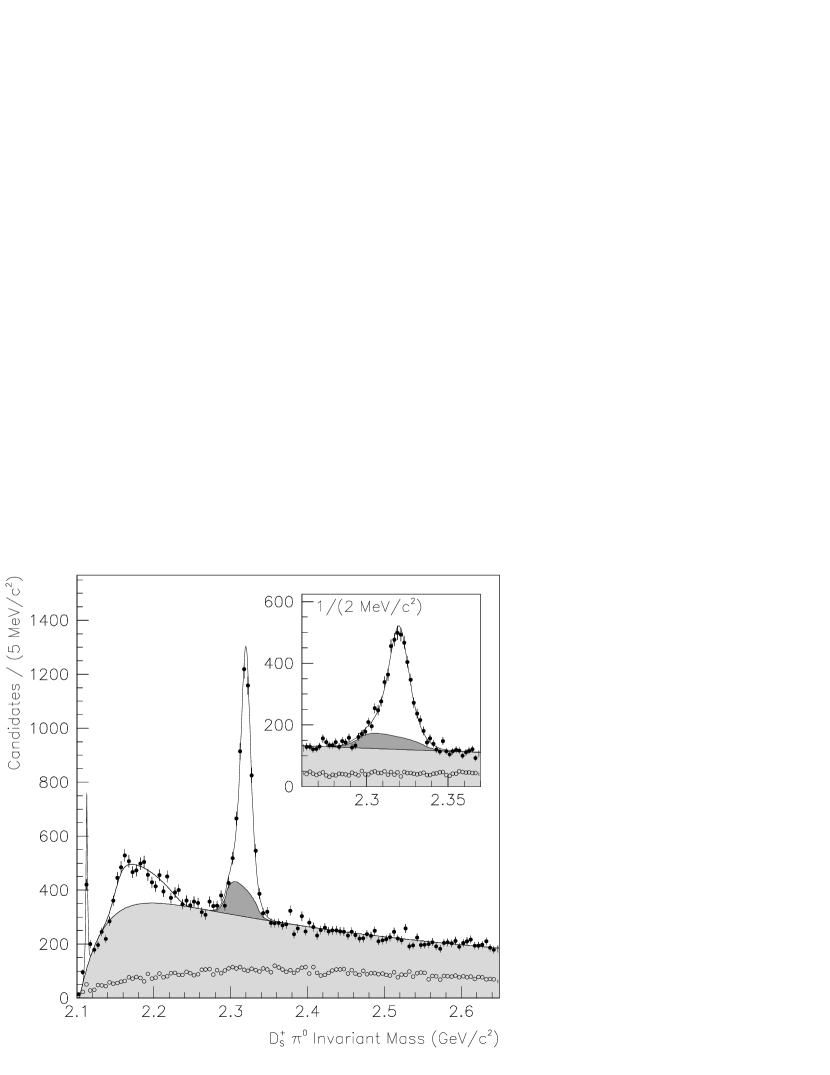
Figure 7: The invariant mass distribution for (solid points) $D^{+}_{s}\pi^{0}$ candidates and (open points) the equivalent using the $D^{+}_{s}$ sidebands. The curve represents the likelihood fit described in the text. Included in this fit is (light shade) a contribution from combinatorial background and (dark shade) the reflection from $D_{sJ}(2460)^{+}\to D_{s}^{*}(2112)^{+}\pi^{0}$ decay. The insert highlights the details near the $D_{sJ}^{*}(2317)^{+}$ mass.

As shown in Fig. 8(a), the reconstructed mass distribution of the $D_{sJ}^{*}(2317)^{+}\to D^{+}_{s}\pi^{0}$ decay, as predicted by MC, has non-Gaussian tails and is slightly asymmetric. To describe this shape, the MC sample is fit to a modified Lorentzian function $F_{L}(m)$:

$$F_{L}(m) = a_{3}\frac{\left|1+a_{4}\delta+a_{5}\delta^{3}\right|}{\left(1+\delta^{2}\right)^{a_{6}}}$$ (11)

$$\delta \equiv \left(m-a_{1}\right)/a_{2}\;,$$

where $a_{1}$ and $a_{2}$ correspond roughly to a mean and width, respectively. This function is simply a convenient parameterization of detector resolution. The fit results are shown in Fig. 8(a). A similar procedure is used for the hypothetical $D_{sJ}(2460)^{+}\to D^{+}_{s}\pi^{0}$ decay (Fig. 8(b)).

Figure 8: The reconstructed $D^{+}_{s}\pi^{0}$ invariant mass spectrum from (a) $D_{sJ}^{*}(2317)^{+}$ and (b) $D_{sJ}(2460)^{+}$ MC samples. The fit function of Eq. 11 is overlaid. (c) The projection of $D^{+}_{s}\pi^{0}$ mass for subresonant $D_{sJ}(2460)^{+}$ decay through the $D_{s}^{*}(2112)^{+}$ meson is restricted to a narrow range centered around 2313.4 ${\mathrm{\,Me\kern-1.00006ptV\!/}c^{2}}$. (d) The reconstructed $D^{+}_{s}\pi^{0}$ invariant mass spectrum for the $D_{sJ}(2460)^{+}$ reflection from MC simulation. The solid curve is the fit function. The dashed curve is the same fit function with the Gaussian smearing removed.

The 350 ${\mathrm{\,Me\kern-1.00006ptV\!/}c}$  $\pi^{0}$ momentum requirement removes the majority of $D_{s}^{*}(2112)^{+}\to D^{+}_{s}\pi^{0}$ decays. The remaining signal is modeled using a distribution $J(m)$ of Gaussians:

$$J(m)=a_{1}\int_{a_{3}}^{a_{3}a_{4}}\frac{1}{a_{4}\sigma^{2}}\!\exp\left[-(m-a_{2})^{2}/2\sigma^{2}\right]\text{d}\sigma\;.$$ (12)

The parameters $a_{3}$ and $a_{4}$ of this function are determined using a fit to a suitable MC sample. The mean mass $a_{2}$ is set equal to $2112.9$ ${\mathrm{\,Me\kern-1.00006ptV\!/}c^{2}}$  (0.5 ${\mathrm{\,Me\kern-1.00006ptV\!/}c^{2}}$ higher than the PDG value Eidelman et al. (2004)) to match the data.

A reflection in $D^{+}_{s}\pi^{0}$ produced by $D_{s}^{*}(2112)^{+}\to D^{+}_{s}\gamma$ decay appears as a broad distribution peaking at a mass of approximately 2.17 ${\mathrm{\,Ge\kern-1.00006ptV\!/}c^{2}}$. This reflection is produced by fake $\pi^{0}$ candidates consisting of the $\gamma$ particle from $D_{s}^{*}(2112)^{+}$ decay combined with unassociated $\gamma$ candidates. Kinematics limit this reflection to $D^{+}_{s}\pi^{0}$ masses above the quadrature sum of $D^{+}_{s}$ and $\pi^{0}$ meson masses (approximately 2.1167 ${\mathrm{\,Ge\kern-1.00006ptV\!/}c^{2}}$). This distribution falls gradually as mass is increased due to the rapidly falling inclusive $\gamma$ energy spectrum. Detector resolution tends to smear the lower kinematic mass limit. To model this reflection, a quadratic function with a sharp lower mass cut off is convoluted with a Gaussian distribution. The parameters of this function are determined directly from the $D^{+}_{s}\pi^{0}$ data sample.

The $D_{sJ}(2460)^{+}$ reflection requires careful attention because it appears directly under the $D_{sJ}^{*}(2317)^{+}$ signal. This reflection is produced by the $D^{+}_{s}\pi^{0}$ projection of $D_{sJ}(2460)^{+}\to D_{s}^{*}(2112)^{+}\pi^{0}$ decay (in which the $\gamma$ from $D_{s}^{*}(2112)^{+}$ decay is ignored). A kinematic calculation (Fig. 8(c)) of the $D_{sJ}(2460)^{+}$ Dalitz distribution predicts that this reflection, at the limit of perfect resolution and efficiency, is a flat distribution in mass squared centered at a $D^{+}_{s}\pi^{0}$ mass of 2313.4 ${\mathrm{\,Me\kern-1.00006ptV\!/}c^{2}}$  with a full width of 41.3 ${\mathrm{\,Me\kern-1.00006ptV\!/}c^{2}}$  (assuming a $D_{sJ}(2460)^{+}$ mass of 2458.0 ${\mathrm{\,Me\kern-1.00006ptV\!/}c^{2}}$).

The $D_{sJ}(2460)^{+}$ reflection is flat in mass squared only if the $\pi^{0}$ efficiency is constant. In practice this is not the case, as illustrated by MC simulation (Fig. 8(d)). To accommodate the non-constant efficiency, the $D^{+}_{s}\pi^{0}$ mass distribution from the MC sample is fit to a function consisting of a bounded quadratic function smeared by a double Gaussian. The result of the fit is shown in Fig. 8d.

The threshold function $C(m)$ of Eq. 8 is used to represent the mass spectrum from combinatorial background where the threshold value $a_{1}$ is fixed to 2103.5 ${\mathrm{\,Me\kern-1.00006ptV\!/}c^{2}}$, the sum of the assumed $D^{+}_{s}$ and $\pi^{0}$ masses. The remaining parameters of $C(m)$ are determined directly from the data.

The results of the likelihood fit to the $D^{+}_{s}\pi^{0}$ mass spectrum is shown in Fig. 7. In this fit, the size, shape, and mean mass of the $D_{sJ}(2460)^{+}$ reflection are fixed to values consistent with the yield and mass results determined in Section XI of this paper. The yield of $D_{s}^{*}(2112)^{+}$ and $D_{sJ}^{*}(2317)^{+}$ decay and the $D_{sJ}^{*}(2317)^{+}$ mass is allowed to vary to best match the data. A $D_{sJ}^{*}(2317)^{+}$ mass of $(2319.6\pm 0.2)$ ${\mathrm{\,Me\kern-1.00006ptV\!/}c^{2}}$  is obtained (statistical error only). A total of $3180\pm 80$ $D_{sJ}^{*}(2317)^{+}$ decays are found.

The fit includes a hypothetical contribution from $D_{sJ}(2460)^{+}\to D^{+}_{s}\pi^{0}$ in the form of a line shape of fixed shape and mass. The result is a yield of $-40\pm 50$ (statistical errors only). The size of this yield is small enough that the curve cannot be distinguished in Fig. 7.

The $D_{sJ}(2460)^{+}$ reflection arises from contamination from $D_{s}^{*}(2112)^{+}$ decay. It is an interesting exercise to identify and separate some of this background. This can be accomplished by searching for any $\gamma$ candidates that, when combined with the $D^{+}_{s}$ in the same event, produce a $D^{+}_{s}\gamma$ mass within 15 ${\mathrm{\,Me\kern-1.00006ptV\!/}c^{2}}$  of the $D_{s}^{*}(2112)^{+}$ mass. Those $D^{+}_{s}\pi^{0}$ combinations in which such a match is not found will contain a smaller proportion of $D_{sJ}(2460)^{+}$ reflection, whereas the remaining $D^{+}_{s}\pi^{0}$ combinations will contain fewer $D_{sJ}^{*}(2317)^{+}$ decays. This is indeed the case as illustrated in Fig. 9. The same likelihood fit procedure used for the entire sample is repeated for these $D^{+}_{s}\pi^{0}$ subsamples, including the MC prediction of the yield and shape of the $D_{sJ}(2460)^{+}$ reflection. The fit results are consistent with the data.

Figure 9: Fit results near the $D_{sJ}^{*}(2317)^{+}$ peak for the $D^{+}_{s}\pi^{0}$ sample divided into combinations (a) with and (b) without a $D^{+}_{s}$ consistent with $D_{s}^{*}(2112)^{+}\to D^{+}_{s}\gamma$ decay. The curves and shaded regions, as described in Fig. 7, represent the result of a likelihood fit.

As can be seen in Figs. 7 and 9, the $D_{sJ}^{*}(2317)^{+}$ line shape derived from MC simulation and used unchanged in the likelihood describes the data well. Since the MC simulation is configured with an intrinsic width (0.1 $\mathrm{\,Me\kern-1.00006ptV}$) nearly indistinguishable from zero, it follows that the data are consistent with a zero width $D_{sJ}^{*}(2317)^{+}$ meson.

To extract a 95% CL upper limit on the intrinsic $D_{sJ}^{*}(2317)^{+}$ width, the $D_{sJ}^{*}(2317)^{+}$ line shape is convolved with a relativistic Breit-Wigner function $\sigma_{J}(m)$ with constant width $\Gamma$:

$$\sigma_{J}(m)\propto\frac{m_{0}\Gamma}{\left(m_{0}^{2}-m^{2}\right)^{2}+m_{0}^{2}\Gamma^{2}}\;.$$ (13)

The fit is then repeated in its entirety at incremental steps in $\Gamma$ to produce a likelihood curve. Integrating this curve as a function of $\Gamma$ produces a 95% CL upper limit of $\Gamma<1.9$ $\mathrm{\,Me\kern-1.00006ptV}$ (statistical error only).

In order to produce an estimate of $D_{sJ}^{*}(2317)^{+}$ yield, the fit results must be corrected for selection efficiency. This efficiency is calculated using a $D_{sJ}^{*}(2317)^{+}$ MC sample and is $p^{*}$ dependent. Since the $p^{*}$ distribution observed in data does not exactly match the MC simulation, it is important to take into account this $p^{*}$ dependence. Two methods are used to do this. The first is to weight each $D^{+}_{s}\pi^{0}$ combination by the inverse of the selection efficiency before applying a likelihood fit. After correcting for absolute $D^{+}_{s}\to\phi\pi^{+}$ yield (Section VI), the result is:

$$N(D_{sJ}^{*}(2317)^{+}\to D^{+}_{s}\pi^{0},D^{+}_{s}\to\phi\pi^{+})=26~{}290\pm 650$$

for $p^{*}>3.2$ ${\mathrm{\,Ge\kern-1.00006ptV\!/}c}$ (statistical error only).

The second method is to divide the $D^{+}_{s}\pi^{0}$ sample into bins of $p^{*}$. A likelihood fit is applied to each bin and the yield corrected for the average selection efficiency in that bin. The result is the $p^{*}$ distribution shown in Fig. 10. The total yield from this method is $26470\pm 660$ (statistical error only).

Figure 10: Corrected $D_{sJ}^{*}(2317)^{+}\to D^{+}_{s}\pi^{0}$ yield as a function of $p^{*}$.

The systematic uncertainties for the $D_{sJ}^{*}(2317)^{+}$ mass and yield are summarized in Table 3. The uncertainties in $D_{sJ}(2460)^{+}$ yield are calculated in the same fashion. The assumed $D^{+}_{s}$ mass value and the 1% relative uncertainty in the EMC energy scale are the two largest contributors to the error on the $D_{sJ}^{*}(2317)^{+}$ mass. Uncertainties in the signal shape produce the largest uncertainties in $D_{sJ}^{*}(2317)^{+}$ yield and width.

For example, the amount of $D_{sJ}(2460)^{+}$ reflection is proportional to the $D_{sJ}(2460)^{+}$ yield, which, as will be discussed in Section XI, has an 11% uncertainty. Adjusting the contribution of this reflection in the fit with no other changes produces a relative uncertainty of 2.0% in the $D_{sJ}^{*}(2317)^{+}$ yield with little change in the $D_{sJ}^{*}(2317)^{+}$ mass and width limit. If the likelihood fit is allowed to choose a $D_{sJ}(2460)^{+}$ reflection yield that best matches the data, little change in either the $D_{sJ}^{*}(2317)^{+}$ mass or yield is observed. The limit on the intrinsic width, however, increases to 3.4 $\mathrm{\,Me\kern-1.00006ptV}$, since reducing the $D_{sJ}(2460)^{+}$ reflection allows the observed mass line shape to accommodate a larger intrinsic $D_{sJ}^{*}(2317)^{+}$ width.

Another uncertainty that has a similar effect is the assumed $D^{+}_{s}\pi^{0}$ mass resolution. Small variations in resolution, consistent with comparisons of data and MC simulation of other known particles, can change the $D_{sJ}^{*}(2317)^{+}$ line shape sufficiently to lower or raise yields by 3.2%. Allowing better reconstructed resolution provides more room for a large intrinsic width, raising the 95% CL for $\Gamma$ to 3.0 $\mathrm{\,Me\kern-1.00006ptV}$.

Other uncertainties in the $D_{sJ}^{*}(2317)^{+}$ yield include the accuracy ($\pm 3$%) of the MC prediction of $\pi^{0}$ efficiency, the difference of the two methods for correcting for $p^{*}$-dependent efficiency, and the $D^{+}_{s}\to\phi\pi^{+}$ branching fraction. The total systematic uncertainty is calculated from the quadrature sum of all sources. The result is the following $D_{sJ}^{*}(2317)^{+}$ mass:

$$m=(2319.6\pm 0.2\;(\text{stat.})\pm 1.4\;(\text{syst.}))\;\text{${\mathrm{\,Me\kern-1.00006ptV\!/}c^{2}}$}\;,$$

and the following yields:

$$\begin{array}[]{lcl@{}r@{\:}c@{\:}r@{\:}c@{\:}r@{}l}\bar{\sigma}(D_{sJ}^{*}(2317)^{+}\to D^{+}_{s}\pi^{0})&=&(&115.8\>&\pm\hfil\>&2.9\>&\pm\hfil\>&8.7&)\;\text{fb}\\ \bar{\sigma}(D_{sJ}(2460)^{+}\to D^{+}_{s}\pi^{0})&=&(&-1.0\>&\pm\hfil\>&1.4\>&\pm\hfil\>&0.1&)\;\text{fb},\end{array}$$

where the first error is statistical and the second is systematic.

Table 3: A summary of systematic uncertainties for the $D_{sJ}^{*}(2317)^{+}$ mass and yield from the analysis of the $D^{+}_{s}\pi^{0}$ final state.

	Mass	Relative
Source	(${\mathrm{\,Me\kern-1.00006ptV\!/}c^{2}}$)	yield (%)
$D^{+}_{s}$ mass	0.6	—
EMC energy scale	1.3	—
$D_{sJ}(2460)^{+}$ reflection size	$<0.1$	2.0
$D_{sJ}(2460)^{+}$ mass	0.1	0.7
Detector resolution	$<0.1$	3.2
$D_{s}^{*}(2112)^{+}$ reflection model	$<0.1$	0.4
$D^{+}_{s}$ efficiency	—	3.9
$\pi^{0}$ efficiency	—	3.0
$p^{*}$ distribution	—	0.6
$D^{+}_{s}\to\phi\pi^{+}$ yield	—	3.9
Quadrature sum	1.4	7.4

As can be seen in Table 3, the determination of the $D_{sJ}^{*}(2317)^{+}$ mass is limited by the understanding of the EMC energy scale. A more primitive calculation of this energy scale was used in a previous estimate of the $D_{sJ}^{*}(2317)^{+}$ mass from this collaboration Aubert et al. (2004a), resulting in an mass estimate that is 2.3 ${\mathrm{\,Me\kern-1.00006ptV\!/}c^{2}}$ lighter then the estimate presented here. The associated systematic uncertainty in this previous work was also incorrectly calculated. The central value and systematic uncertainty in mass reported here reflects the current best understanding of these calibration issues.

For the sake of simplicity, in order to incorporate systematic effects into a limit on $\Gamma$, the least strict limit obtained from the various systematic checks is quoted. This produces a 95% CL of $\Gamma<3.8$ $\mathrm{\,Me\kern-1.00006ptV}$. The lineshape produced by this limit is illustrated in Fig. 11.

Figure 11: Likelihood fit results for a $D_{sJ}^{*}(2317)^{+}$ meson of instrinsic width (dashed line) $\Gamma=0$ and (solid line) $\Gamma=3.8$ $\mathrm{\,Me\kern-1.00006ptV}$. Shown in comparison is the mass distribution (solid points) for the $D^{+}_{s}\pi^{0}$ candidates.

X The $D^{+}_{s}\gamma$ Final State

The $D^{+}_{s}\gamma$ mass distribution using $\gamma$ candidates with loose (150 $\mathrm{\,Me\kern-1.00006ptV}$) and final (500 $\mathrm{\,Me\kern-1.00006ptV}$) minimum energy requirements is shown in Fig. 12. Some structure in the vicinity of the $D_{sJ}^{*}(2317)^{+}$ and $D_{sJ}(2460)^{+}$ masses becomes apparent once the tighter energy requirements are applied. The looser requirement is useful for studying the $D_{s}^{*}(2112)^{+}$ peak. A fit to that peak consisting of two Gaussians on top of a polynomial background function results in a peak $D_{s}^{*}(2112)^{+}$ mass of $2113.8$ ${\mathrm{\,Me\kern-1.00006ptV\!/}c^{2}}$  and a yield of 75 000 decays, both with negligible statistical uncertainties.

Figure 12: The invariant $D^{+}_{s}\gamma$ mass distribution using $\gamma$ candidates with loose (150 $\mathrm{\,Me\kern-1.00006ptV}$) and final (500 $\mathrm{\,Me\kern-1.00006ptV}$) energy requirements. The insert focuses on the region of the $D_{s}^{*}(2112)^{+}$ meson using the loose energy requirement. The curve represents the fit described in the text.

An unbinned likelihood fit is applied to the final $D^{+}_{s}\gamma$ mass distribution in order to extract the parameters and yield of the $D_{sJ}(2460)^{+}$ meson and upper limits on $D_{sJ}^{*}(2317)^{+}$ decay. For simplicity, the fit is performed only for masses between 2.15 and 2.85 ${\mathrm{\,Ge\kern-1.00006ptV\!/}c^{2}}$. The likelihood fit includes five distinct sources of $D^{+}_{s}\gamma$ combinations:

• $D_{sJ}(2460)^{+}\to D^{+}_{s}\gamma$ decay.

• $D_{sJ}^{*}(2317)^{+}\to D^{+}_{s}\gamma$ decay (hypothetical).

• A reflection from $D_{sJ}^{*}(2317)^{+}\to D^{+}_{s}\pi^{0}$ decay in which only one of the $\gamma$ particles from $\pi^{0}$ decay is included.

• A reflection from $D_{sJ}(2460)^{+}\to D_{s}^{*}(2112)^{+}\pi^{0}$ decay in which only one of the $\gamma$ particles from $\pi^{0}$ decay is included.

• Background from both unassociated $D^{+}_{s}$ and $\gamma$ mesons and the high-mass tail from $D_{s}^{*}(2112)^{+}\to D^{+}_{s}\gamma$ decay.

The PDF used to describe the mass distribution of each of these sources is described below.

As shown in Fig. 13(b), the reconstructed mass distribution of the $D_{sJ}(2460)^{+}\to D^{+}_{s}\gamma$ decay, as predicted by MC, has a long, low mass tail. To describe this shape, the MC sample is fit to a modified Lorentzian function $F_{L2}(m)$:

$$F_{L2}(m) = a_{3}\frac{\left|1+a_{4}\delta+a_{5}\delta^{2}+a_{6}\delta^{3}\right|}{\left(1+\delta^{2}\right)^{a_{7}}}$$ (14)

$$\delta \equiv \left(m-a_{1}\right)/a_{2}\;.$$

The fit results are shown in Fig. 13(b). A similar procedure is used for the hypothetical $D_{sJ}^{*}(2317)^{+}\to D^{+}_{s}\gamma$ decay (Fig. 13(a)).

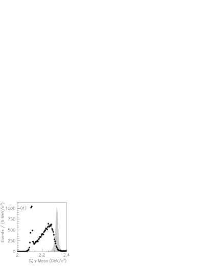
Figure 13: The reconstructed $D^{+}_{s}\gamma$ invariant mass spectrum from MC samples for (a) $D_{sJ}^{*}(2317)^{+}$ and (b) $D_{sJ}(2460)^{+}$ decay and (c) $D_{sJ}^{*}(2317)^{+}\to D^{+}_{s}\pi^{0}$ and (d) $D_{sJ}(2460)^{+}\to D_{s}^{*}(2112)^{+}\pi^{0}$ reflections. The curves are the fit functions described in the text. The $D_{sJ}^{*}(2317)^{+}$ signal shapes from (a) and (b) are shown for comparison in (c) and (d) in gray.

Ignoring resolution effects, the $D_{sJ}^{*}(2317)^{+}$ reflection produces an invariant $D^{+}_{s}\gamma$ mass distribution up to a maximum of approximately 140 ${\mathrm{\,Me\kern-1.00006ptV\!/}c^{2}}$  below the $D_{sJ}^{*}(2317)^{+}$ mass. Candidate selection requirements produce a distribution that peaks at this limit. Resolution effects smear this sharp peak producing the shape shown in Fig. 13(c), as predicted by MC. This distribution can be reasonably described (in the mass range of interest) by a bounded quadratic function convoluted with a double Gaussian. The $D_{sJ}(2460)^{+}$ reflection has a similar behavior near the $D_{sJ}^{*}(2317)^{+}$ mass (Fig. 13(d)). Both distributions overlap the direct $D_{sJ}^{*}(2317)^{+}\to D^{+}_{s}\gamma$ decay.

The following function $D(m)$ is used to represent the remainder of the $D^{+}_{s}\gamma$ distribution:

$$D(m)=1+a_{1}\exp\left[-\right(m-a_{3}\left){}^{2}/a_{2}\right]\;.$$ (15)

This includes combinatorial background along with any tail from $D_{s}^{*}(2112)^{+}\to D^{+}_{s}\gamma$ decay. The MC simulation fails to reproduce the shape of this background, either due to unknown $c\bar{s}$ contributions (for example, higher resonant states) or unexpected behavior of the tail of the distribution from $D_{s}^{*}(2112)^{+}$ decay. This issue, combined with the complex shapes associated with the $D_{sJ}^{*}(2317)^{+}$ and $D_{sJ}(2460)^{+}$ reflections, leads to considerable systematic uncertainty in the fit. Likelihood fits under several different conditions are attempted in order to understand the uncertainty.

One fit that produces a good representation of the data is shown in Fig. 14. In this fit, all parameters except the upper mass limit of the $D_{sJ}^{*}(2317)^{+}$ reflection are allowed to vary. The estimated raw $D_{sJ}(2460)^{+}$ ($D_{sJ}^{*}(2317)^{+}$) yield from this fit is $920\pm 60$ ($-130\pm 130$). The fitted $D_{sJ}(2460)^{+}$ mass is $(2459.5\pm 1.2)$ ${\mathrm{\,Me\kern-1.00006ptV\!/}c^{2}}$ (statistical errors only).

Figure 14: An example likelihood fit to the $D^{+}_{s}\gamma$ invariant mass distribution. The solid points in the top plot are the mass distribution. The open points are the $D^{+}_{s}$ sidebands, scaled appropriately. The bottom plot shows the same data after subtracting the background curve from the fit. Various contributions to the likelihood fit are also shown.

The $D_{sJ}(2460)^{+}$ signal is far enough removed from the $D_{sJ}^{*}(2317)^{+}$ and $D_{sJ}(2460)^{+}$ reflections that accurate mass and yield results are obtained. The same two methods described in the previous section are used to estimate the $D_{sJ}(2460)^{+}$ yield. The first method, using $p^{*}$ dependent weights proportional to the inverse of efficiency, produces a corrected yield of:

$$N(D_{sJ}(2460)^{+}\to D^{+}_{s}\gamma,D^{+}_{s}\to\phi\pi^{+})=3270\pm 230$$

for $p^{*}>3.2$ ${\mathrm{\,Ge\kern-1.00006ptV\!/}c}$ (statistical error only). The second method produces the $p^{*}$ spectrum shown in Fig. 15. The total yield from the spectrum is $3080\pm 240$ (statistical error only), approximately 6.2% lower than the first estimate.

Figure 15: Corrected $D_{sJ}(2460)^{+}\to D^{+}_{s}\gamma$ yield as a function of $p^{*}$.

Systematic uncertainties associated with the assumed PDFs for the background and reflection shapes are explored using different variations of the likelihood fit. Among the variations applied is an alternate description of the background shape:

$$D^{\prime}(m)=1+a_{1}\exp\left[-5\right(m-a_{3}\left)\right]+a_{2}/\left(m-a_{3}\right)^{2}\;.$$ (16)

In addition, the MC predictions for the size and shape of the $D_{sJ}^{*}(2317)^{+}$ reflection are used unaltered (despite producing a fit of inferior quality). Large variations of raw $D_{sJ}^{*}(2317)^{+}$ yield of up to 490 events are observed.

The shape of the $D_{sJ}(2460)^{+}\to D^{+}_{s}\gamma$ signal is sensitive to several factors that are difficult to simulate exactly, including EMC energy resolution. Variations in the assumed resolution are used to study the associated systematic uncertainty in yield and mass. The result is an uncertainty of 3.5% in yield and no significant change in mass.

All systematic uncertainties for the $D_{sJ}(2460)^{+}$ mass and yield are listed in Table 4. The result is the following $D_{sJ}(2460)^{+}$ mass:

$$m=(2459.5\pm 1.2\;(\text{stat.})\pm 3.7\;(\text{syst.}))\;\text{${\mathrm{\,Me\kern-1.00006ptV\!/}c^{2}}$}\;,$$

and the following yields:

$$\begin{array}[]{lcl@{}r@{\:}c@{\:}r@{\:}c@{\:}r@{}l}\bar{\sigma}(D_{sJ}^{*}(2317)^{+}\to D^{+}_{s}\gamma)&=&(&-2.4\>&\pm\hfil\>&2.3\>&\pm\hfil\>&8.9&)\;\text{fb}\\ \bar{\sigma}(D_{sJ}(2460)^{+}\to D^{+}_{s}\gamma)&=&(&14.4\>&\pm\hfil\>&1.0\>&\pm\hfil\>&1.4&)\;\text{fb},\end{array}$$

where the first error is statistical and the second is systematic.

Table 4: A summary of systematic uncertainties for the $D_{sJ}(2460)^{+}$ mass and yield from the analysis of the $D^{+}_{s}\gamma$ final state.

	Mass	Relative
Source	(${\mathrm{\,Me\kern-1.00006ptV\!/}c^{2}}$)	yield (%)
$D^{+}_{s}$ mass	0.6	—
EMC energy scale	3.7	—
$D_{sJ}^{*}(2317)^{+}$ mass	0.1	$0.1$
$D_{sJ}^{*}(2317)^{+}$ reflection shape	0.1	$1.9$
Detector resolution	$<0.1$	$3.5$
Background shape	0.5	$3.3$
$D^{+}_{s}$ efficiency	—	$3.9$
$\gamma$ efficiency	$<0.1$	$1.8$
$p^{*}$ distribution	—	$6.3$
$D^{+}_{s}\to\phi\pi^{+}$ branching fraction	—	$3.9$
Quadrature sum	3.7	$10.0$

XI The $D^{+}_{s}\pi^{0}\gamma$ Final State

The invariant mass spectrum for all selected $D^{+}_{s}\pi^{0}\gamma$ candidates is shown in Fig. 16(a). A $D_{sJ}(2460)^{+}$ signal is apparent. The shape of this signal is characterized by applying the following modified Lorentzian fit function $F_{L3}$:

$$F_{L3}(m) = a_{3}\frac{\left|1+a_{4}\delta+a_{5}\tan^{-1}5\delta\right|}{\left(1+\delta^{2}\right)^{a_{6}}}$$ (17)

$$\delta \equiv \left(m-a_{1}\right)/a_{2}\;.$$

to a $D_{sJ}(2460)^{+}\to D_{s}^{*}(2112)^{+}\pi^{0}$ MC sample (Fig. 16(b)). A binned $\chi^{2}$ fit to the $D^{+}_{s}\pi^{0}\gamma$ spectrum that includes this shape along with a polynomial description of the background produces a $D_{sJ}(2460)^{+}$ mass $(2459.5\pm 2.0)$ ${\mathrm{\,Me\kern-1.00006ptV\!/}c^{2}}$  and a yield of $560\pm 80$ events (statistical errors only).

Figure 16: (a) The sample of $D^{+}_{s}\pi^{0}\gamma$ candidates shown in solid points. The fit described in the text is overlaid. The open points are those candidates which fall in a restricted $D^{+}_{s}\gamma$ mass range. (b) The reconstructed $D^{+}_{s}\pi^{0}\gamma$ invariant mass spectrum from a $D_{sJ}(2460)^{+}\to D_{s}^{*}(2112)^{+}\pi^{0}$ MC sample. The fit function of Eq. 17 is overlaid.

In the following, it is assumed that the $D_{sJ}(2460)^{+}$ meson decays to $D^{+}_{s}\pi^{0}\gamma$ entirely through either of the two kinematically allowed sub-resonant decay modes:

$$D_{sJ}(2460)^{+}\to\left\{\begin{array}[]{c}D_{s}^{*}(2112)^{+}\pi^{0}\\ D_{sJ}^{*}(2317)^{+}\gamma\end{array}\right\}\to D^{+}_{s}\pi^{0}\gamma$$ (18)

Due to a kinematic accident, the phase space of these two sub-resonant modes overlap, as illustrated in Fig. 17. It is therefore possible to remove background while retaining both sub-resonant decay modes by selecting $D^{+}_{s}\pi^{0}\gamma$ candidates in either a restricted range of $D^{+}_{s}\pi^{0}$ mass or a restricted range of $D^{+}_{s}\gamma$ mass. This analysis uses a requirement that the $D^{+}_{s}\gamma$ mass must be within 20 ${\mathrm{\,Me\kern-1.00006ptV\!/}c^{2}}$  of the $D_{s}^{*}(2112)^{+}$ mass. As shown in Fig. 16(a), the resulting $D^{+}_{s}\pi^{0}\gamma$ mass distribution in this $D^{+}_{s}\gamma$ signal window is considerably cleaner.

Figure 17: The light gray region indicates the range of $D^{+}_{s}\pi^{0}$ and $D^{+}_{s}\gamma$ mass that is kinematically allowed in the decay of an object of mass $2458.0$ ${\mathrm{\,Me\kern-1.00006ptV\!/}c^{2}}$ to $D^{+}_{s}\pi^{0}\gamma$. The lines mark the kinematic space associated with decays which proceed through an intermediate $D_{s}^{*}(2112)^{+}$ or $D_{sJ}^{*}(2317)^{+}$ meson.

The $D^{+}_{s}\gamma$ requirement introduces a source of background that peaks underneath the $D_{sJ}(2460)^{+}$ signal. This background is a reflection from $D_{sJ}^{*}(2317)^{+}\to D^{+}_{s}\pi^{0}$ decays that are not associated with any $D_{sJ}(2460)^{+}$ decay. The reflection arises because, as illustrated in Fig. 17, any $D_{sJ}^{*}(2317)^{+}$ signal that is combined with a $\gamma$ candidate that produces a $D^{+}_{s}\gamma$ mass near the $D_{s}^{*}(2112)^{+}$ meson results in a $D^{+}_{s}\pi^{0}\gamma$ mass near the $D_{sJ}(2460)^{+}$ meson. If the $D^{+}_{s}\gamma$ mass requirement is shifted upwards or downwards, this $D_{sJ}^{*}(2317)^{+}$ reflection shifts up and down in $D^{+}_{s}\pi^{0}\gamma$ mass by a predictable amount.

Another type of background that behaves similarly to the $D_{sJ}^{*}(2317)^{+}$ reflection is $D_{sJ}(2460)^{+}\to D^{+}_{s}\pi^{0}\gamma$ decay in which the wrong $\gamma$ candidate is chosen. This type of background is slightly wider and smaller than the $D_{sJ}^{*}(2317)^{+}$ reflection, but otherwise has a similar mass distribution. To describe this background contribution, it is assumed that the $D_{sJ}(2460)^{+}$ decays entirely through $D_{s}^{*}(2112)^{+}\pi^{0}$ and is produced at a rate comparable to previous measurements. Both assumptions need not be entirely accurate since this background has a relatively small contribution.

To characterize the $D_{sJ}^{*}(2317)^{+}$ and $D_{sJ}(2460)^{+}$ reflections, upper and lower $D^{+}_{s}\gamma$ mass selection windows are chosen centered at $\pm 60$ ${\mathrm{\,Me\kern-1.00006ptV\!/}c^{2}}$  away from the $D_{s}^{*}(2112)^{+}$ mass. The mass distribution from MC samples of $D_{sJ}^{*}(2317)^{+}\to D^{+}_{s}\pi^{0}$ and $D_{sJ}(2460)^{+}\to D_{s}^{*}(2112)^{+}\gamma$ decay are shown in Fig. 18 for the signal and two sideband $D^{+}_{s}\gamma$ mass windows. The shape of the two combined reflections in all three cases can be successfully described by a fit to a Gaussian.

Figure 18: The combined $D^{+}_{s}\pi^{0}\gamma$ invariant mass distribution (solid points) as obtained from MC samples for the combination of the $D_{sJ}^{*}(2317)^{+}$ reflection and $D_{sJ}(2460)^{+}\to D_{s}^{*}(2112)^{+}\pi^{0}$ decays in which the incorrect $\gamma$ is chosen. The $D_{sJ}(2460)^{+}$ contribution alone is shown in open points. Shown are the (a) upper, (b) signal, and (c) lower $D^{+}_{s}\gamma$ mass selection windows. The curves are fits to Gaussian distributions.

To determine the mass, width, and yield of the $D_{sJ}(2460)^{+}$ meson, an unbinned likelihood fit is applied to the $D^{+}_{s}\pi^{0}\gamma$ mass distribution of candidates selected in the $D^{+}_{s}\gamma$ signal window. This fit includes the following contributions:

• $D_{sJ}(2460)^{+}\to D^{+}_{s}\pi^{0}\gamma$ decay.

• The combined reflections from $D_{sJ}^{*}(2317)^{+}\to D^{+}_{s}\pi^{0}$ decay and from $D_{sJ}(2460)^{+}\to D_{s}^{*}(2112)^{+}\gamma$ decay in which the incorrect $\gamma$ candidate is chosen.

• A reflection from $D_{s}^{*}(2112)^{+}\to D^{+}_{s}\gamma$ decay in which an unassociated $\gamma$ candidate is added to form a fake $\pi^{0}$ candidate.

• Smooth background sources that do not have any peaking behavior.

The $D_{s}^{*}(2112)^{+}\to D^{+}_{s}\gamma$ reflection is similar to that observed in $D^{+}_{s}\pi^{0}$ combinations (see, for example, Fig. 7). The smooth background is represented by the $C(m)$ function described in Eq. 8.

Two similar fits excluding the $D_{sJ}(2460)^{+}$ signal are applied to the upper and lower $D^{+}_{s}\gamma$ mass samples. These fits suggest that the MC prediction of the absolute rate of the $D_{s}^{*}(2112)^{+}\to D^{+}_{s}\gamma$ reflection is approximately 21% too low. The fit models are adjusted accordingly. The fit results for all three $D^{+}_{s}\gamma$ mass ranges after this adjustment are shown in Fig. 19. The result is a $D_{sJ}(2460)^{+}$ mass of $(2458.6\pm 1.3)$ ${\mathrm{\,Me\kern-1.00006ptV\!/}c^{2}}$  and a raw yield of $560\pm 40$ events (statistical errors only).

Although the overall size of the $D_{sJ}^{*}(2317)^{+}\to D^{+}_{s}\pi^{0}$ reflection is allowed to vary, the MC prediction for the relative contributions in the three $D^{+}_{s}\gamma$ mass windows is preserved. Since the size of this reflection is adequately modeled in the two $D^{+}_{s}\gamma$ sidebands, there is some confidence that the size is well established in the $D^{+}_{s}\gamma$ signal window.

Note that the size of the smooth background is relatively larger in the signal $D^{+}_{s}\gamma$ window due to contributions from $D_{s}^{*}(2112)^{+}\to D^{+}_{s}\gamma$ decay. In addition, if there were significant non-resonant contributions to $D_{sJ}(2460)^{+}$ decay, peaks at the $D_{sJ}(2460)^{+}$ mass would be visible in the two $D^{+}_{s}\gamma$ sidebands. No such evidence is visible.

Figure 19: The invariant mass distribution of $D^{+}_{s}\pi^{0}\gamma$ candidates in the (a) upper, (b) signal, and (c) lower $D^{+}_{s}\gamma$ mass selection windows for (solid points) the $D^{+}_{s}$ signal and (open points) $D^{+}_{s}$ sideband samples. The curves represent the fits described in the text. The dark gray (light gray) region corresponds to the predicted contribution from the $D_{sJ}^{*}(2317)^{+}$ ($D_{s}^{*}(2112)^{+}$) reflection.

The two methods described in the two previous sections are used to estimate the $D_{sJ}(2460)^{+}$ yield. The first method, using $p^{*}$ dependent weights proportional to the inverse of efficiency, produces a corrected yield of:

$$N(D_{sJ}(2460)^{+}\to D^{+}_{s}\pi^{0}\gamma,D^{+}_{s}\to\phi\pi^{+})=9690\pm 790$$

for $p^{*}>3.2$ ${\mathrm{\,Ge\kern-1.00006ptV\!/}c}$ (statistical error only). The second method produces the $p^{*}$ spectrum shown in Fig. 20. The total yield from the spectrum is $9890\pm 810$ (statistical error only).

Figure 20: Corrected $D_{sJ}(2460)^{+}\to D^{+}_{s}\pi^{0}\gamma$ yield as a function of $p^{*}$.

The systematic uncertainties in the mass and yield of the $D_{sJ}(2460)^{+}$ meson are shown in Table 5. As described previously, the size of the $D_{sJ}^{*}(2317)^{+}$ reflection was adjusted in the fit to match the $D^{+}_{s}\gamma$ sideband samples. If the size of the reflection is taken unchanged from MC predictions, the $D_{sJ}(2460)^{+}$ yield increases by 7.3%. A second likelihood fit described later in this section used to distinguish between the two $D_{sJ}(2460)^{+}$ sub-resonant decay modes also produces an estimate of $D_{sJ}(2460)^{+}$ yield. The difference between the two fits is treated as a systematic uncertainty. The total $D_{sJ}(2460)^{+}$ yield, without distinguishing between the two possible sub-resonant decay modes, is measured to be

$$\bar{\sigma}(D_{sJ}(2460)^{+}\to D^{+}_{s}\pi^{0}\gamma)=(42.7\pm 3.5\pm 4.2)\;\text{fb},$$

where the first error is statistical and the second is systematic. The complete $D_{sJ}(2460)^{+}$ mass result is:

$$m=(2458.6\pm 1.0\;(\text{stat.})\pm 2.5\;(\text{syst.}))\;\text{${\mathrm{\,Me\kern-1.00006ptV\!/}c^{2}}$}\;.$$

Table 5: A summary of systematic uncertainties for the $D_{sJ}(2460)^{+}$ mass and yield from the analysis of the $D^{+}_{s}\pi^{0}\gamma$ final state.

	Mass	Relative
Source	(${\mathrm{\,Me\kern-1.00006ptV\!/}c^{2}}$)	yield (%)
$D^{+}_{s}$ mass	0.6	—
EMC energy scale	2.4	—
$D_{sJ}^{*}(2317)^{+}$ reflection size	0.3	7.3
$D_{sJ}^{*}(2317)^{+}$ mass	0.1	1.2
Detector resolution	$<0.1$	2.1
$D_{s}^{*}(2112)^{+}$ reflection model	—	—
Fit method	—	1.4
$D^{+}_{s}$ efficiency	—	3.9
$\pi^{0}$ and $\gamma$ efficiency	—	3.0
$p^{*}$ distribution	—	2.1
$D^{+}_{s}\to\phi\pi^{+}$ yield	—	3.9
Quadrature sum	2.5	10.2

The $D_{sJ}(2460)^{+}$ signal PDF used in the likelihood fit of Fig. 19 includes a $D_{sJ}(2460)^{+}$ intrinsic width of $\Gamma=0.1$ $\mathrm{\,Me\kern-1.00006ptV}$. Larger intrinsic widths do not result in any significant improvement of the fit. After applying the same likelihood-integration technique described in Section IX for the $D^{+}_{s}\pi^{0}$ final state, and including the systematic effects listed in Table 5, the result is a 95% CL limit of $\Gamma<6.3$ $\mathrm{\,Me\kern-1.00006ptV}$.

Having established a $D_{sJ}(2460)^{+}\to D^{+}_{s}\pi^{0}\gamma$ signal, it is now necessary to distinguish between the two possible sub-resonant decay modes shown in Eq. 18. These two decay modes can be distinguished by their $D^{+}_{s}\pi^{0}$ and $D^{+}_{s}\gamma$ invariant mass distributions, as shown in Fig. 21. The distributions for the $D_{sJ}(2460)^{+}\to D_{s}^{*}(2112)^{+}\pi^{0}$ subresonant mode are determined using a MC sample. The reconstructed $D^{+}_{s}\gamma$ mass distribution, which is relatively narrow (as it arises from $D_{s}^{*}(2112)^{+}$ decay), is represented by a $\chi^{2}$ fit to the $F_{L3}$ function (Eq. 17). The wider $D^{+}_{s}\pi^{0}$ mass distribution is accurately modeled by a square function smeared by a double Gaussian. Both fits are shown in Fig. 21.

In contrast, for the $D_{sJ}(2460)^{+}\to D_{sJ}^{*}(2317)^{+}\gamma$ subresonant decay mode, the $D^{+}_{s}\pi^{0}$ mass distribution is narrow and the $D^{+}_{s}\gamma$ mass distribution is wide. The $D^{+}_{s}\pi^{0}$ distribution is determined using a $D_{sJ}^{*}(2317)^{+}\to D^{+}_{s}\pi^{0}$ MC sample. The $D^{+}_{s}\gamma$ distribution is calculated using the parameters determined from the $D^{+}_{s}\pi^{0}$ distribution from $D_{sJ}(2460)^{+}\to D_{s}^{*}(2112)^{+}\pi^{0}$ described above converted to the appropriate kinematic range. The shapes assumed for both $D_{sJ}(2460)^{+}\to D_{sJ}^{*}(2317)^{+}\gamma$ mass projections are shown in gray in Fig. 21.

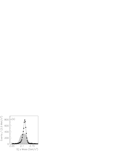
Figure 21: The reconstructed (a) $D^{+}_{s}\pi^{0}$ and (b) $D^{+}_{s}\gamma$ invariant mass distributions for the two possible $D_{sJ}(2460)^{+}$ sub-resonant decay modes. The distributions from a $D_{sJ}(2460)^{+}\to D_{s}^{*}(2112)^{+}\pi^{0}$ MC sample are shown in points. The curves are the fits described in the text. The shaded regions are the shapes assumed for $D_{sJ}(2460)^{+}\to D_{sJ}^{*}(2317)^{+}\gamma$ decay.

The $D^{+}_{s}\pi^{0}$ and $D^{+}_{s}\gamma$ mass distributions of the signal cannot be explored without correctly subtracting backgrounds from unassociated $D_{s}^{*}(2112)^{+}\to D^{+}_{s}\gamma$ and $D_{sJ}^{*}(2317)^{+}\to D^{+}_{s}\pi^{0}$ decay. This subtraction is performed by a two-dimensional unbinned likelihood fit applied to the $D^{+}_{s}\pi^{0}$ and $D^{+}_{s}\gamma$ mass distributions of the data. The likelihood fit is restricted to the data sample contained inside the grid shown in Fig. 22. This fit includes five sources of $D^{+}_{s}\pi^{0}\gamma$ candidates:

• Combinatorial background represented by a two-dimensional quadratic function.

• Background from $D_{s}^{*}(2112)^{+}\to D^{+}_{s}\gamma$ decay combined with unassociated $\pi^{0}$ candidates represented by a $D_{s}^{*}(2112)^{+}$ line shape in the $D^{+}_{s}\gamma$ mass and as a linear function in $D^{+}_{s}\pi^{0}$ mass.

• Background from $D_{sJ}^{*}(2317)^{+}\to D^{+}_{s}\pi^{0}$ decay combined with unassociated $\gamma$ candidates represented by a $D_{sJ}^{*}(2317)^{+}$ line shape in the $D^{+}_{s}\pi^{0}$ mass and as a linear function in $D^{+}_{s}\gamma$ mass.

• A signal from $D_{sJ}(2460)^{+}\to D_{s}^{*}(2112)^{+}\pi^{0}$ with $D^{+}_{s}\pi^{0}$ and $D^{+}_{s}\gamma$ mass distributions represented by the curves in Fig. 21.

• A signal from $D_{sJ}(2460)^{+}\to D_{sJ}^{*}(2317)^{+}\gamma$ with $D^{+}_{s}\pi^{0}$ and $D^{+}_{s}\gamma$ mass distributions represented by the gray regions in Fig. 21.

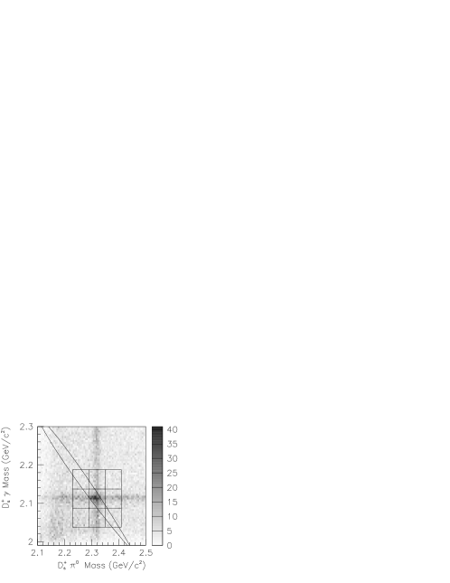
Figure 22: The $D^{+}_{s}\gamma$ versus $D^{+}_{s}\pi^{0}$ mass distributions for the $D^{+}_{s}\pi^{0}\gamma$ candidates. The horizontal (vertical) band corresponds to background from $D_{s}^{*}(2112)^{+}\to D^{+}_{s}\gamma$ ($D_{sJ}^{*}(2317)^{+}\to D^{+}_{s}\pi^{0}$) decay. The excess of candidates near the crossing of these two bands is the $D_{sJ}(2460)^{+}$ signal. The curve indicates the region of phase space in which the $D_{sJ}(2460)^{+}$ decay is kinematically restricted. The grid identifies the subsample of candidates used in the likelihood fit shown in Fig. 23.

The result of this likelihood fit is shown in Fig. 23, divided into the regions delineated by the grid shown in Fig. 22. The fit produces an adequate model of the data in all regions. The result (statistical errors only) is a total yield of $520\pm 50$ $D_{sJ}(2460)^{+}\to D^{+}_{s}\pi^{0}\gamma$ decays with a fraction of ($2.5\pm 8.8$)% proceeding through the $D_{sJ}^{*}(2317)^{+}\gamma$ channel, the former number being somewhat smaller than the yield determined by the $D^{+}_{s}\pi^{0}\gamma$ mass fit (Fig. 19), though consistent within systematic uncertainties. Based on these results, it appears that the decay $D_{sJ}(2460)^{+}\to D^{+}_{s}\pi^{0}\gamma$ can be successfully described as proceeding entirely through the channel $D_{s}^{*}(2112)^{+}\pi^{0}$.

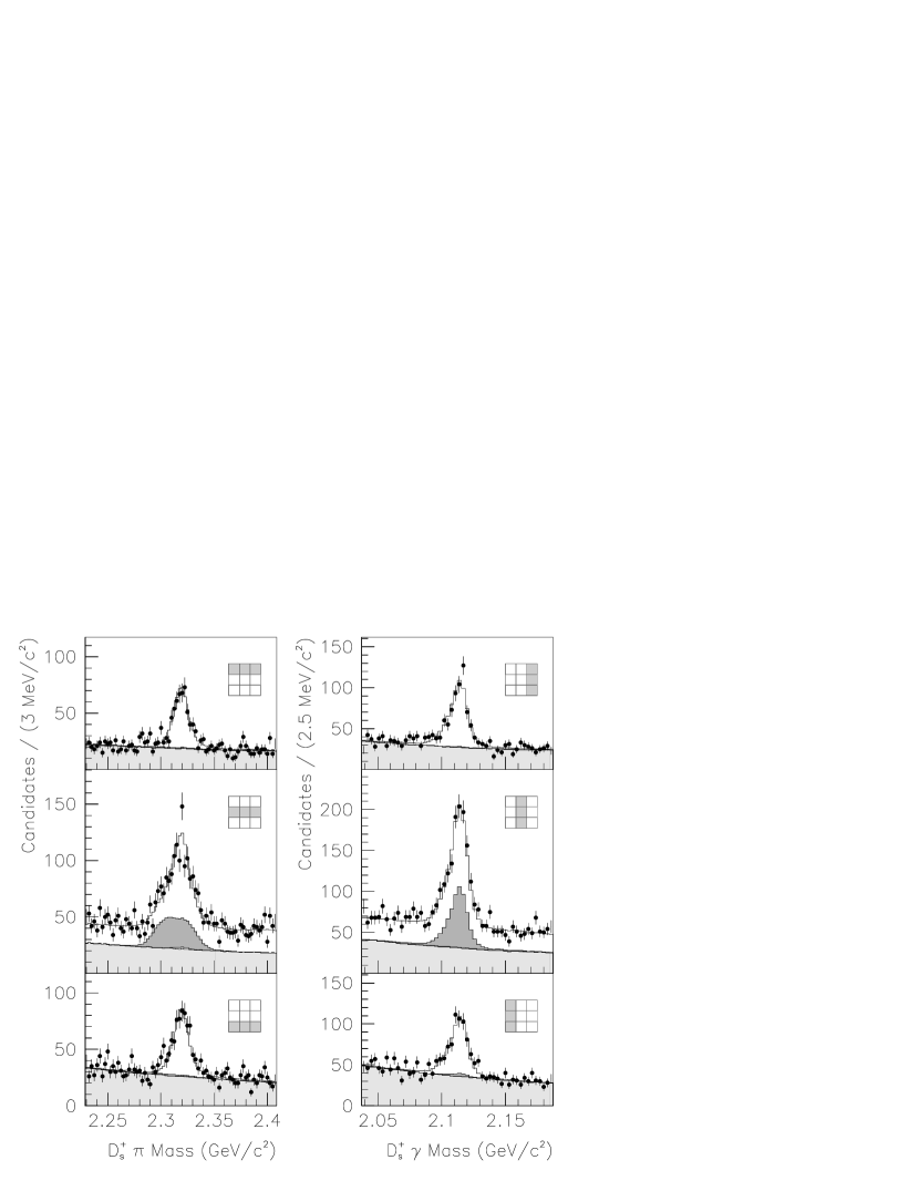
Figure 23: The $D^{+}_{s}\pi^{0}$ and $D^{+}_{s}\gamma$ invariant mass distributions for $D^{+}_{s}\pi^{0}\gamma$ candidates that fall within the indicated portions of the grid shown in Fig. 22. The histograms represent the results of a likelihood fit. The light gray region corresponds to combinatorial background. The medium gray (dark gray) region represents the fitted fraction of $D_{sJ}(2460)^{+}\to D_{s}^{*}(2112)^{+}\pi^{0}$ ($D_{sJ}(2460)^{+}\to D_{sJ}^{*}(2317)^{+}\gamma$).

The systematic uncertainties listed in Table 5 can be applied to the above fit results. In combination with the results of the fit to the $D^{+}_{s}\pi^{0}\gamma$ mass distribution of Fig. 19, and treating correlated systematic uncertainties in the appropriate fashion, the following yields for the subresonant specific decays are obtained:

$$\begin{array}[]{lcl@{}r@{\:}c@{\:}r@{\:}c@{\:}r@{}l}\bar{\sigma}(D_{sJ}(2460)^{+}\to D_{s}^{*}(2112)^{+}\pi^{0})&=&(&41.6\>&\pm\hfil\>&5.1\>&\pm\hfil\>&5.0&)\;\text{fb}\\ \bar{\sigma}(D_{sJ}(2460)^{+}\to D_{sJ}^{*}(2317)^{+}\gamma)&=&(&1.1\>&\pm\hfil\>&5.1\>&\pm\hfil\>&5.0&)\;\text{fb},\end{array}$$

where the first error is statistical and the second is systematic.

A simple helicity analysis is used to test the $J^{P}$ assignment of the $D_{sJ}(2460)^{+}$ meson under the assumption that the decay $D_{sJ}(2460)^{+}\to D^{+}_{s}\pi^{0}\gamma$ proceeds entirely through the subresonant mode $D_{s}^{*}(2112)^{+}\pi^{0}$. This analysis is performed in terms of the helicity angle $\vartheta_{h}$, defined as the angle of the $\gamma$ in the $D_{s}^{*}(2112)^{+}$ center-of-mass frame with respect to the $D_{s}^{*}(2112)^{+}$ direction. Since the $D_{s}^{*}(2112)^{+}$ is a vector particle, the helicity distribution must consist of some combination of the zero helicity distribution $H_{0}$:

$$H_{0}=\sin^{2}\vartheta_{h}$$ (19)

and the helicity = $\pm 1$ distribution $H_{1}$:

$$H_{1}=\frac{1}{2}\left(1+\cos^{2}\vartheta_{h}\right)\;.$$ (20)

As listed in Table 6, the expected combination of $H_{0}$ and $H_{1}$ depends on the assumed $D_{sJ}(2460)^{+}$ spin and parity.

Table 6: Helicity distributions in the decay $D_{sJ}(2460)^{+}\to D_{s}^{*}(2112)^{+}\pi^{0}$ for hypothetical $D_{sJ}(2460)^{+}$ spin-parity assignments.

$J^{P}$	Helicity Distribution
$0^{+}$	(decay is forbidden)
$0^{-}$	$H_{0}$
$1^{-},2^{+},3^{-},4^{+},\ldots$	$H_{1}$
$1^{+},2^{-},3^{+},4^{-},\ldots$	any combination of $H_{0}$ and $H_{1}$

To measure the helicity distribution, the $D^{+}_{s}\pi^{0}\gamma$ candidates are divided into five bins of $\cos\vartheta_{h}$. The $D^{+}_{s}\pi^{0}\gamma$ mass fit of Fig. 19 is repeated for each of these subsamples using $p^{*}$-dependent weights inversely proportional to the selection efficiency in order to correct for acceptance. The result is shown in Fig. 24. The integral of the following function is calculated in each $\cos\vartheta_{h}$ bin:

$$F_{h}=a_{1}\left[\left(1-a_{2}\right)H_{0}+a_{2}H_{1}\right]\;.$$ (21)

A $\chi^{2}$ fit is used to determine the most likely value of $a_{2}$. The result is $a_{2}=0.76\pm 0.14$ (statistical errors only).

The same procedure can be repeated after each relevant systematic check listed in Table 5 is performed. The differences in $a_{2}$ values so obtained are added in quadrature to estimate the total systematic uncertainty. The final result is:

$$a_{2}=0.76\pm 0.14\;(\text{stat.})\pm 0.06\;(\text{syst})\;,$$ (22)

where $a_{2}=0$ ($a_{2}=1$) corresponds to a $D_{sJ}(2460)^{+}$ of helicity zero ($\pm 1$). This value of $a_{2}$ deviates from zero by 5.1 standard deviations, which strongly disfavors the $J^{P}=0^{-}$ interpretation of the $D_{sJ}(2460)^{+}$ while remaining consistent with a $J=1$ or higher interpretation of either parity

Figure 24: Efficiency-corrected yields in five $\cos\vartheta_{h}$ bins for the decay $D_{sJ}(2460)^{+}\to D_{s}^{*}(2112)^{+}\pi^{0}$. The solid histogram is the result of a fit to the function described in the text. The dashed histogram is a similar fit with the $a_{2}$ parameter fixed to zero.

XII The $D^{+}_{s}\pi^{0}\pi^{0}$ Final State

The $D^{+}_{s}\pi^{0}\pi^{0}$ final state contains potential contributions from $D_{sJ}(2460)^{+}\to D_{s}^{*}(2112)^{+}\pi^{0}$ subresonant decay through the channel $D_{s}^{*}(2112)^{+}\to D^{+}_{s}\pi^{0}$, which has a branching ratio of 5.8% Eidelman et al. (2004). Since this sub-resonant mode is more efficiently investigated using the $D^{+}_{s}\pi^{0}\gamma$ final state (as discussed in the previous section), it is removed from the $D^{+}_{s}\pi^{0}\pi^{0}$ sample by requiring the $D^{+}_{s}\pi^{0}$ invariant mass to be greater than 2117.4 ${\mathrm{\,Me\kern-1.00006ptV\!/}c^{2}}$  for both $\pi^{0}$ candidates. This requirement excludes the edges of the $D_{sJ}^{*}(2317)^{+}$ and $D_{sJ}(2460)^{+}$ phase spaces, as illustrated in Fig. 25. This figure also demonstrates how little phase space is available to the $D_{sJ}^{*}(2317)^{+}$ meson in this decay in comparison to the $D_{sJ}(2460)^{+}$ meson.

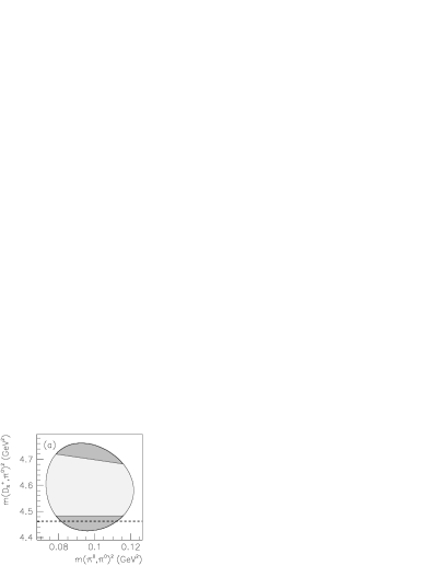
Figure 25: The Dalitz phase space available to (a) the $D_{sJ}^{*}(2317)^{+}$ and (b) the $D_{sJ}(2460)^{+}$ mesons in the $D^{+}_{s}\pi^{0}\pi^{0}$ final state. The dashed horizontal line corresponds to the $D_{s}^{*}(2112)^{+}$ mass. The dark shaded regions are those parts of the phase space removed by the requirement $m(D^{+}_{s}\pi^{0})>2117.4$ ${\mathrm{\,Me\kern-1.00006ptV\!/}c^{2}}$. The dotted curve in (b) is the $D_{sJ}^{*}(2317)^{+}$ phase space drawn for comparison.

The invariant mass distribution of the selected $D^{+}_{s}\pi^{0}\pi^{0}$ candidates is shown in Fig. 26. There is no evidence of $D_{sJ}^{*}(2317)^{+}$ or $D_{sJ}(2460)^{+}$ meson decay, nor is there evidence of any structure in the background. The mass distribution is fit using a likelihood function that consists of the smooth background function $C(m)$ (Eq. 8) and $D_{sJ}^{*}(2317)^{+}$ and $D_{sJ}(2460)^{+}$ meson contributions, the latter two having yields that are allowed to fluctuate to negative values. The shape of the signals is modeled by double Gaussians, the parameters of which are determined by fits to MC samples. The masses of the $D_{sJ}^{*}(2317)^{+}$ and $D_{sJ}(2460)^{+}$ mesons are fixed to values measured in the previous sections.

Figure 26: The invariant mass distribution for (solid points) $D^{+}_{s}\pi^{0}\pi^{0}$ candidates and (open points) the equivalent using the $D^{+}_{s}$ sidebands. The curve represents the likelihood fit described in the text. The insert focuses on the low mass region. The dotted line in the insert indicates the $D_{sJ}^{*}(2317)^{+}$ mass.

The result of the likelihood fit is shown in Fig. 26 and produces a $D_{sJ}^{*}(2317)^{+}$ ($D_{sJ}(2460)^{+}$) raw yield of $0.2\pm 3.9$ ($5\pm 10$) (statistical errors only). Efficiency corrections are calculated by applying a $D^{+}_{s}\pi^{0}\pi^{0}$ candidate weight that is inversely proportional to $p^{*}$-dependent selection efficiency, calculated from MC samples. This procedure produces corrected $D_{sJ}^{*}(2317)^{+}$ and $D_{sJ}(2460)^{+}$ meson yields of $1900\pm 1600$ and $1300\pm 1200$, respectively (statistical errors only).

Various systematic uncertainties are considered. According to MC simulation, the selection efficiency varies by as much as 20% across the Dalitz plot. Since no specific Dalitz distribution is assumed, this variation is translated directly into a multiplicative systematic uncertainty. An alternate shape $C^{\prime}_{2}(m)$ for the background is considered:

$$C^{\prime}_{2}(m)=\sqrt{m^{2}-a_{1}^{2}}\left(1+a_{2}m+a_{3}m^{3}\right)\;.$$ (23)

A fit with this background increases the raw $D_{sJ}^{*}(2317)^{+}$ yield by 0.5 events. Detector resolution and $D_{sJ}^{*}(2317)^{+}$ and $D_{sJ}(2460)^{+}$ meson mass variations have similar effects. The final results are

$$\begin{array}[]{lcl@{}r@{\:}c@{\:}r@{\:}c@{\:}r@{}l}\bar{\sigma}(D_{sJ}^{*}(2317)^{+}\to D^{+}_{s}\pi^{0}\pi^{0})&=&(&8.7\>&\pm\hfil\>&6.9\>&\pm\hfil\>&5.0&)\;\text{fb}\\ \bar{\sigma}(D_{sJ}(2460)^{+}\to D^{+}_{s}\pi^{0}\pi^{0})&=&(&5.5\>&\pm\hfil\>&5.4\>&\pm\hfil\>&2.4&)\;\text{fb},\end{array}$$

where the first error is statistical and the second is systematic.

XIII The $D^{+}_{s}\gamma\gamma$ Final State

It is assumed that there are three possible contributions to the decay of the $D_{sJ}^{*}(2317)^{+}$ and $D_{sJ}(2460)^{+}$ mesons to the $D^{+}_{s}\gamma\gamma$ final state:

• Two body decay to $D^{+}_{s}\pi^{0}$ followed by $\pi^{0}\to\gamma\gamma$.

• Subresonant decay to $D_{s}^{*}(2112)^{+}\gamma$ followed by $D_{s}^{*}(2112)^{+}\to D^{+}_{s}\gamma$.

• Non-resonant decay directly to $D^{+}_{s}\gamma\gamma$.

The $D^{+}_{s}\pi^{0}$ final state, already studied in Section IX, is removed from the $D^{+}_{s}\gamma\gamma$ sample by the $\gamma$ selection requirements. Potential background from $\pi^{0}$ mass tails is removed by further requiring the $\gamma\gamma$ invariant mass to be less than 100 ${\mathrm{\,Me\kern-1.00006ptV\!/}c^{2}}$  or greater than 170 ${\mathrm{\,Me\kern-1.00006ptV\!/}c^{2}}$. The remaining two $D^{+}_{s}\gamma\gamma$ contributions are treated by dividing the sample into two portions, one rich in $D_{s}^{*}(2112)^{+}$ decay (referred to as the $D_{s}^{*}(2112)^{+}$ sample), and the remainder (referred to as the non-resonant sample). A $D^{+}_{s}\gamma\gamma$ candidate is placed in the $D_{s}^{*}(2112)^{+}$ sample if either $\gamma$ produces a $D^{+}_{s}\gamma$ invariant mass within 15 ${\mathrm{\,Me\kern-1.00006ptV\!/}c^{2}}$  of the PDG value for the $D_{s}^{*}(2112)^{+}$ mass (2112.4 ${\mathrm{\,Me\kern-1.00006ptV\!/}c^{2}}$) Eidelman et al. (2004).

Figure 27 illustrates how the the $D^{+}_{s}\gamma\gamma$ candidates are divided in terms of the phase space of $D_{sJ}^{*}(2317)^{+}$ and $D_{sJ}(2460)^{+}$ meson decay. The $D^{+}_{s}\gamma\gamma$ invariant mass distribution of the two samples is shown in Fig. 28. No clear $D_{sJ}^{*}(2317)^{+}$ or $D_{sJ}(2460)^{+}$ signal is observed. The mass distributions contain structure associated both with the $\pi^{0}$ veto requirements and with the $D_{s}^{*}(2112)^{+}$ sample selection requirements. Much of this structure can be avoided by applying likelihood fits in a restricted mass range. Two types of background that produce structure that cannot be so avoided are described below.

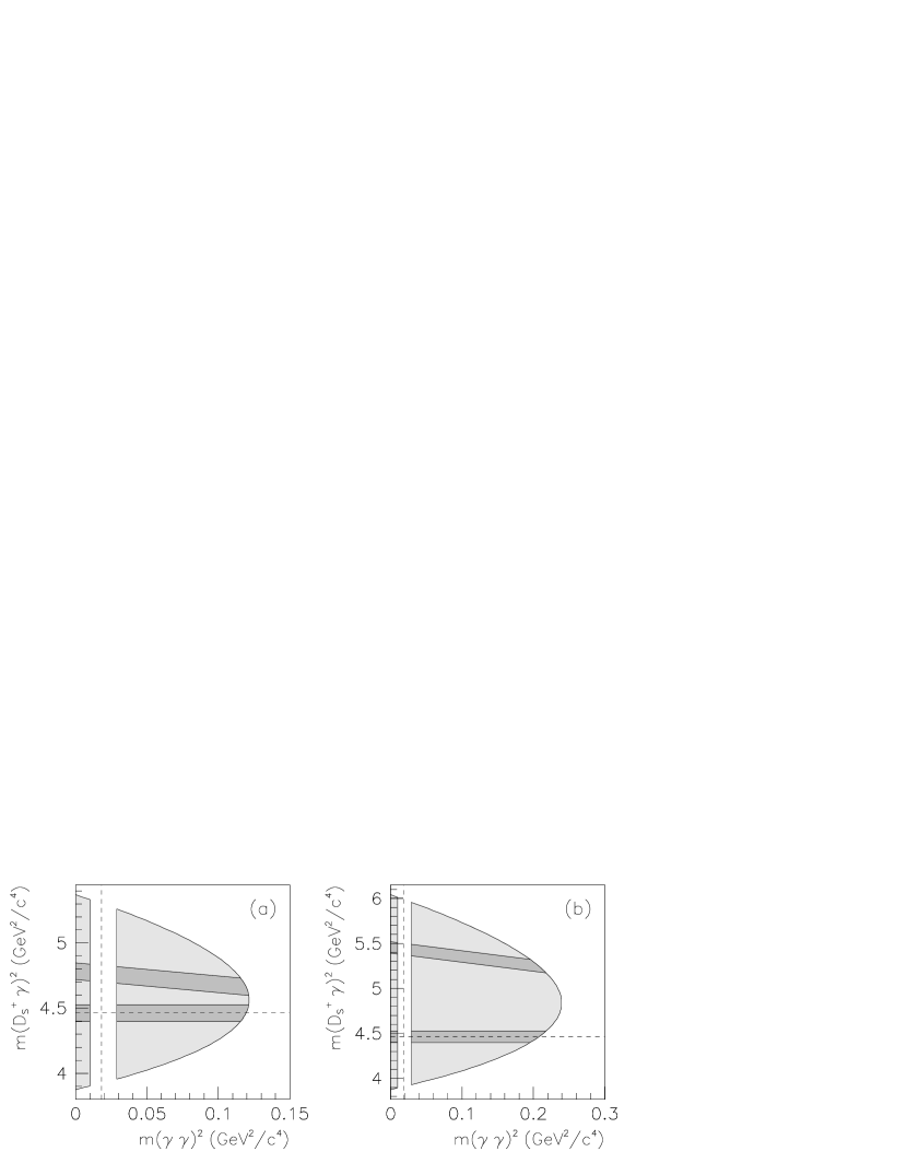
Figure 27: The Dalitz phase space corresponding to the $D^{+}_{s}\gamma\gamma$ samples for (a) $D_{sJ}^{*}(2317)^{+}$ and (b) $D_{sJ}(2460)^{+}$ mesons. The dark shaded and light shaded regions correspond to the $D_{s}^{*}(2112)^{+}$ and non-resonant samples, respectively. The horizontal (vertical) dashed line indicates the $D_{s}^{*}(2112)^{+}$ ($\pi^{0}$) mass.

Figure 28: The $D^{+}_{s}\gamma\gamma$ invariant mass distribution (solid points) for candidates in (a) the $D_{s}^{*}(2112)^{+}$ sample, (b) the non-resonant sample, and (c) either sample. The open points are the corresponding distributions for the $D^{+}_{s}$ sideband. The vertical dashed lines indicate the $D_{sJ}^{*}(2317)^{+}$ and $D_{sJ}(2460)^{+}$ meson masses.

Either of the two $\gamma$ candidates in each $D^{+}_{s}\gamma\gamma$ combination provides two opportunities for the $D^{+}_{s}\gamma\gamma$ combination to be placed into the $D_{s}^{*}(2112)^{+}$ sample. At a specific value of $D^{+}_{s}\gamma\gamma$ invariant mass, however, if one $\gamma$ candidate falls inside the $D_{s}^{*}(2112)^{+}$ mass window, the other $\gamma$ is likely to do the same, due to kinematics. This produces a deficit of candidates at this mass in the $D_{s}^{*}(2112)^{+}$ sample along with a corresponding excess of candidates in the non-resonant sample. The $D^{+}_{s}\gamma\gamma$ invariant mass distribution of this excess can be approximated by the triangular shape centered at 2255.9 ${\mathrm{\,Me\kern-1.00006ptV\!/}c^{2}}$ shown in Fig. 29(a).

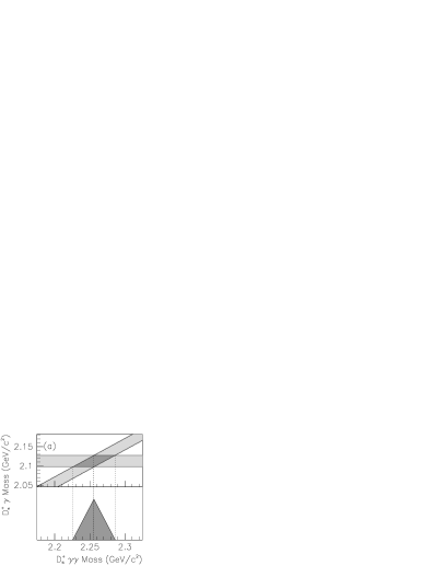
Figure 29: (a) Shown on top as a function of $D^{+}_{s}\gamma$ and $D^{+}_{s}\gamma\gamma$ masses are the bands corresponding to the $D_{s}^{*}(2112)^{+}$ sample requirement ($D^{+}_{s}\gamma$ mass within 15 ${\mathrm{\,Me\kern-1.00006ptV\!/}c^{2}}$  of the $D_{s}^{*}(2112)^{+}$ mass) and the effect of this requirement on the other $\gamma$ candidate. The overlap of the two bands produces the shape shown below. (b) The $D^{+}_{s}\gamma\gamma$ mass distribution of the $D_{sJ}(2460)^{+}\to D_{s}^{*}(2112)^{+}\pi^{0}$ reflection from a MC sample. The curve is the fit described in the text.

The second background source, which only appears in the $D_{s}^{*}(2112)^{+}$ sample, is a reflection from $D_{sJ}(2460)^{+}\to D_{s}^{*}(2112)^{+}\pi^{0}$ decay in which one $\gamma$ particle from the $\pi^{0}$ decay is ignored. This reflection is suppressed but not eliminated by the requirement that each $\gamma$ candidate not belong to a fiducial $\pi^{0}$ candidate. The MC prediction of the shape of this reflection is shown in Fig. 29(b). The shape is accurately modeled by a quadratic polynomial bounded on two sides and smeared by a double Gaussian.

The unbinned maximum-likelihood fit to the $D^{+}_{s}\gamma\gamma$ mass distribution of the $D_{s}^{*}(2112)^{+}$ sample is performed between masses of 2.22 and 2.70 ${\mathrm{\,Ge\kern-1.00006ptV\!/}c^{2}}$. This mass distribution has a cusp near a mass of 2.4 ${\mathrm{\,Ge\kern-1.00006ptV\!/}c^{2}}$  that is difficult to describe using a simple polynomial. Instead, the combinatorial background is parameterized using an empirical function $K(m)$ composed of a line and a parabola that intersect at one point. To make the function smooth, a cubic spline $K_{S}(m)$ is used near the intersection point ($m=a_{1}$) to extrapolate between these two polynomials:

$$K(m)=\left\{\begin{array}[]{ll}a_{2}+a_{3}m&m<a_{1}-\delta\\ K_{S}(m)&\left|m-a_{1}\right|<\delta\\ a_{2}+a_{4}m+a_{5}m^{2}&m>a_{1}+\delta\end{array}\right.\;,$$ (24)

where the value $\delta=20$ ${\mathrm{\,Me\kern-1.00006ptV\!/}c^{2}}$  is chosen to approximately match the resolution.

The reconstructed mass distributions for the hypothetical decay of $D_{sJ}^{*}(2317)^{+}$ and $D_{sJ}(2460)^{+}$ mesons to $D^{+}_{s}\gamma\gamma$ and $D_{s}^{*}(2112)^{+}\gamma$ are modeled by the functional form of Eq 14, the parameters of which are determined by fits to the corresponding MC samples.

The unbinned likelihood fit to the $D^{+}_{s}\gamma\gamma$ mass distribution of the $D_{s}^{*}(2112)^{+}$ sample includes five components:

1. $D_{sJ}^{*}(2317)^{+}\to D_{s}^{*}(2112)^{+}\gamma$ decay (hypothetical).

2. $D_{sJ}(2460)^{+}\to D_{s}^{*}(2112)^{+}\gamma$ decay (hypothetical).

3. A deficit of events of the shape described in Fig. 29(a) but of variable size.

4. A contribution from the $D_{sJ}(2460)^{+}\to D_{s}^{*}(2112)^{+}\pi^{0}$ reflection, of fixed shape based on the fit of Fig. 29(b) and with a yield consistent with the results of Section XI.

5. A background described by the function of Eq. 24.

The result of applying the fit function on the $D_{s}^{*}(2112)^{+}$ sample is shown in Fig. 30. A raw $D_{sJ}^{*}(2317)^{+}$ ($D_{sJ}(2460)^{+}$) yield of $-40\pm 110$ ($-50\pm 140$) is obtained (statistical errors only).

Figure 30: The $D^{+}_{s}\gamma\gamma$ invariant mass distribution for the $D_{s}^{*}(2112)^{+}$ sample is shown on top. The thick curve is the result of the likelihood fit. The mass distribution after subtracting the portion assigned by the fit to combinatorial background is shown on bottom.

The proximity of the $D_{sJ}(2460)^{+}\to D_{s}^{*}(2112)^{+}\pi^{0}$ reflection to potential $D_{sJ}^{*}(2317)^{+}$ and $D_{sJ}(2460)^{+}$ signals coupled with the unknown shape of the combinatorial background leads to large uncertainties in the fit results. For example, if a third-order polynomial is used in place of the function $K(m)$ to describe the smooth background, the $D_{sJ}^{*}(2317)^{+}$ and $D_{sJ}(2460)^{+}$ raw yields increase by 260 and 150 candidates, respectively. Although the result of this fit is a less faithful representation of the mass distribution of the data, as a conservative estimate the entire difference is quoted as a systematic uncertainty. Other systematic checks performed include a variation of the range in $D^{+}_{s}\gamma\gamma$ mass over which the fit is applied, consideration of uncertainties in detector resolution, and variations of the $D_{sJ}^{*}(2317)^{+}$ and $D_{sJ}(2460)^{+}$ masses and the relative size of the $D_{sJ}(2460)^{+}\to D_{s}^{*}(2112)^{+}\pi^{0}$ reflection.

The raw $D_{sJ}^{*}(2317)^{+}$ and $D_{sJ}(2460)^{+}$ yields are corrected for selection efficiency by weighting each $D^{+}_{s}\gamma\gamma$ combination by the inverse of the $p^{*}$-dependent selection efficiency, determined using a MC sample. The results for the $D_{s}^{*}(2112)^{+}\gamma$ final state are:

$$\begin{array}[]{lcl@{}r@{\:}c@{\:}r@{\:}c@{\:}r@{}l}\bar{\sigma}(D_{sJ}^{*}(2317)^{+}\to D_{s}^{*}(2112)^{+}\gamma)&=&(&-0.5\>&\pm\hfil\>&3.2\>&\pm\hfil\>&8.1&)\;\text{fb}\\ \bar{\sigma}(D_{sJ}(2460)^{+}\to D_{s}^{*}(2112)^{+}\gamma)&=&(&-0.9\>&\pm\hfil\>&3.5\>&\pm\hfil\>&4.1&)\;\text{fb},\end{array}$$

where the first error is statistical and the second is systematic.

The $D^{+}_{s}\gamma\gamma$ mass distribution of the phase-space subsample has a cusp that is more pronounced than in the $D_{s}^{*}(2112)^{+}\gamma$ sample but at a mass well below the $D_{sJ}^{*}(2317)^{+}$ mass. This cusp is avoided by restricting the fit to masses above 2.2 ${\mathrm{\,Ge\kern-1.00006ptV\!/}c^{2}}$. In this mass range a simple polynomial is sufficient to describe combinatorial background. The unbinned likelihood fit includes four components:

1. $D_{sJ}^{*}(2317)^{+}\to D^{+}_{s}\gamma\gamma$ decay (hypothetical).

2. $D_{sJ}(2460)^{+}\to D^{+}_{s}\gamma\gamma$ decay (hypothetical).

3. An excess of events of the shape described in Fig. 29(a) but of variable size.

4. Combinatorial background represented by a third-order polynomial.

The result of applying the fit function on the non-resonant sample is shown in Fig. 31. A raw $D_{sJ}^{*}(2317)^{+}$ ($D_{sJ}(2460)^{+}$) yield of $190\pm 120$ ($80\pm 160$) is obtained (statistical errors only).

Figure 31: The $D^{+}_{s}\gamma\gamma$ invariant mass distribution for the non-resonant sample is shown on top. The thick curve is the result of the likelihood fit. The mass distribution after subtracting the portion assigned by the fit to combinatorial background is shown on bottom.

As in the $D_{s}^{*}(2112)^{+}$ sample, raw $D_{sJ}^{*}(2317)^{+}$ and $D_{sJ}(2460)^{+}$ yields are corrected for selection efficiency by weighting each $D^{+}_{s}\gamma\gamma$ combination by the inverse of the $p^{*}$-dependent selection efficiency. This efficiency was determined using a MC sample that simulated the non-resonant decays of the $D_{sJ}^{*}(2317)^{+}$ and $D_{sJ}(2460)^{+}$ mesons to $D^{+}_{s}\gamma\gamma$ using phase space (such that the Dalitz plot was evenly populated). To simulate an alternate decay model, the MC samples were weighted to form a $\cos^{2}\vartheta_{D\gamma}$ distribution, where $\vartheta_{D\gamma}$ is the angle between the $D^{+}_{s}$ and each $\gamma$ in the $D_{sJ}^{*}(2317)^{+}$ and $D_{sJ}(2460)^{+}$ center-of-mass frame. This weighting had the effect of reducing the selection efficiency by 25% and 15% for the $D_{sJ}^{*}(2317)^{+}$ and $D_{sJ}(2460)^{+}$ mesons, respectively.

Other systematic checks include variations in detector resolution, the $D_{sJ}^{*}(2317)^{+}$ and $D_{sJ}(2460)^{+}$ meson masses, and the fit range. The final results for the non-resonant $D^{+}_{s}\gamma\gamma$ final state are:

$$\begin{array}[]{lcl@{}r@{\:}c@{\:}r@{\:}c@{\:}r@{}l}\bar{\sigma}(D_{sJ}^{*}(2317)^{+}\to D^{+}_{s}\gamma\gamma)&=&(&7.4\>&\pm\hfil\>&4.5\>&\pm\hfil\>&2.2&)\;\text{fb}\\ \bar{\sigma}(D_{sJ}(2460)^{+}\to D^{+}_{s}\gamma\gamma)&=&(&3.5\>&\pm\hfil\>&4.3\>&\pm\hfil\>&1.7&)\;\text{fb},\end{array}$$

where the first error is statistical and the second is systematic.

XIV The $D^{+}_{s}\pi^{\pm}$ Final States

The invariant mass distributions of the $D^{+}_{s}\pi^{-}$ and $D^{+}_{s}\pi^{+}$ candidates are shown in Fig. 32 for masses between 2.25 and 2.61 ${\mathrm{\,Ge\kern-1.00006ptV\!/}c^{2}}$. No structure is apparent and both distributions can be adequately described by a second-order polynomial. Since no signal is apparent, the remaining task is to place limits on the yield of hypothetical doubly-charged ($D_{sJ}^{*}(2317)^{++}$) or neutral ($D_{sJ}^{*}(2317)^{0}$) partners of the $D_{sJ}^{*}(2317)^{+}$ meson. To do so requires a few assumptions:

• The intrinsic width $\Gamma$ of either the $D_{sJ}^{*}(2317)^{0}$ or $D_{sJ}^{*}(2317)^{++}$ particle is too small to be resolved by the detector.

• The mass of the $D_{sJ}^{*}(2317)^{0}$ or $D_{sJ}^{*}(2317)^{++}$ particle is within $\pm 10$ ${\mathrm{\,Me\kern-1.00006ptV\!/}c^{2}}$  of the $D_{sJ}^{*}(2317)^{+}$ mass.

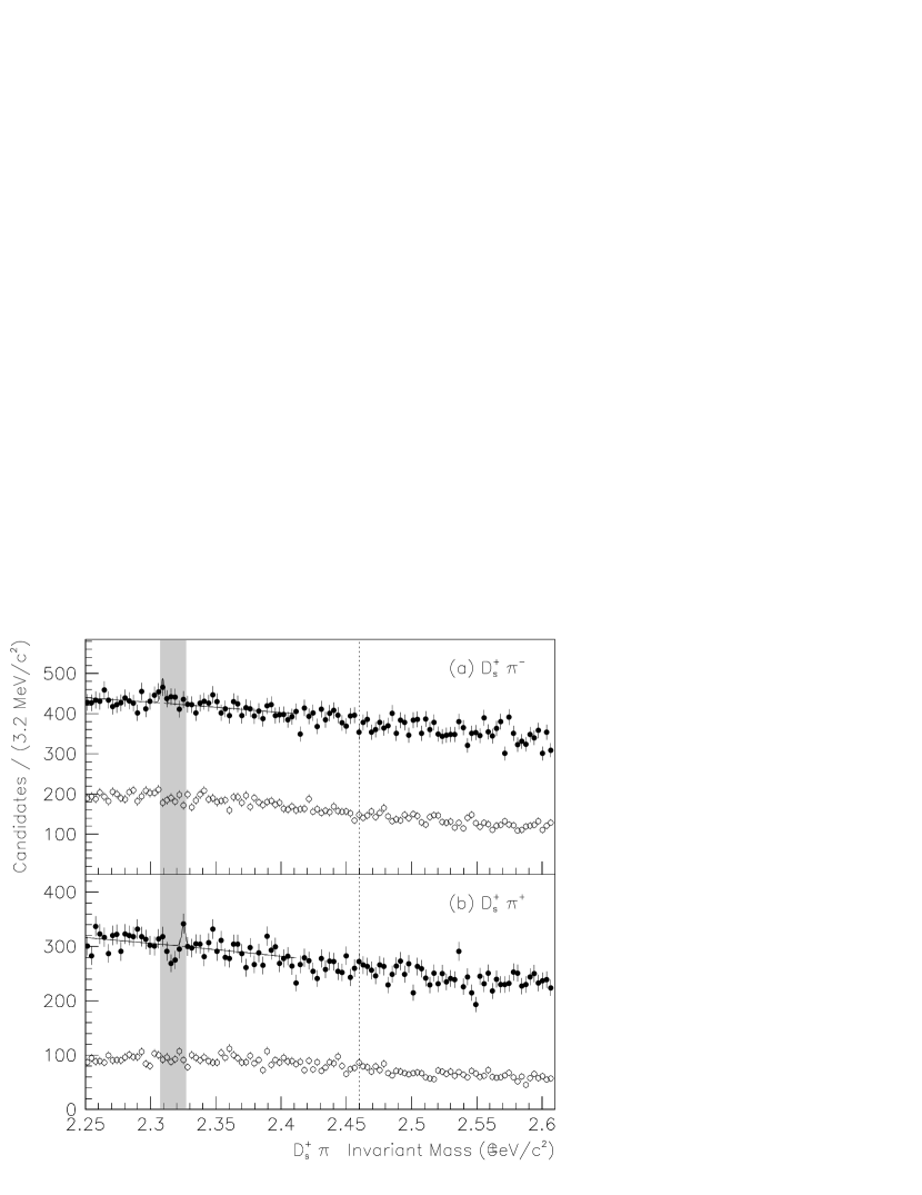
Figure 32: The invariant mass distributions (solids points) of (a) $D^{+}_{s}\pi^{-}$ and (b) $D^{+}_{s}\pi^{+}$ candidates and (open points) the equivalent for the $D^{+}_{s}$ sidebands. The shaded regions indicate the range of assumed $D_{sJ}^{*}(2317)^{++}$ and $D_{sJ}^{*}(2317)^{0}$ masses. The vertical dotted line marks the $D_{sJ}(2460)^{+}$ mass. The curves are the fits described in the text that produce the largest yield within the shaded region.

A series of unbinned likelihood fits based on these assumptions are applied to the $D^{+}_{s}\pi^{-}$ and $D^{+}_{s}\pi^{+}$ mass distributions. Included in these fits is a $D_{sJ}^{*}(2317)^{0}$ or $D_{sJ}^{*}(2317)^{++}$ signal modeled using a line shape extracted from a fit to a $D_{sJ}^{*}(2317)^{0}\to D^{+}_{s}\pi^{-}$ MC sample. According to this fit, the mass resolution is approximately 1.3 ${\mathrm{\,Me\kern-1.00006ptV\!/}c^{2}}$. To avoid potential statistical biases, the mass of each hypothetical particle is fixed at a specific value for each fit. Several such fits are applied with the assumed mass placed between 2307.3 and 2327.3 ${\mathrm{\,Me\kern-1.00006ptV\!/}c^{2}}$  at intervals of 1 ${\mathrm{\,Me\kern-1.00006ptV\!/}c^{2}}$. The fits that produce the largest yields are shown in Fig. 32.

The two final states discussed in this section involve only charged particles and are thus subject to relatively small systematic uncertainties. The largest uncertainty arises from the assumed shape of the background and is estimated by substituting a third-order polynomial for the second-order one. There is also a 1.3% relative uncertainty in the reconstruction efficiency of each $\pi^{\pm}$ candidate. The results from the fits that produce the largest yields are:

$$\begin{array}[]{lcl@{}r@{\:}c@{\:}r@{\:}c@{\:}r@{}l}\bar{\sigma}(D_{sJ}^{*}(2317)^{0}\to D^{+}_{s}\pi^{-})&=&(&1.07\>&\pm\hfil\>&0.44\>&\pm\hfil\>&0.10&)\;\text{fb}\\ \bar{\sigma}(D_{sJ}^{*}(2317)^{++}\to D^{+}_{s}\pi^{+})&=&(&0.74\>&\pm\hfil\>&0.37\>&\pm\hfil\>&0.07&)\;\text{fb},\end{array}$$

where the first error is statistical and the second is systematic. These results will be used to calculate upper limits on the cross section.

XV The $D^{+}_{s}\pi^{+}\pi^{-}$ Final State

The invariant mass distribution of the $D^{+}_{s}\pi^{+}\pi^{-}$ candidates is shown in Fig. 33. Clear peaks from $D_{sJ}(2460)^{+}$ and $D_{s1}(2536)^{+}$ decay are apparent. The distribution has no additional structure of any statistical significance. To determine the mass and yield of the $D_{sJ}(2460)^{+}$ meson, and to place limits on $D_{sJ}^{*}(2317)^{+}$ decay, an unbinned likelihood fit is applied to the $D^{+}_{s}\pi^{+}\pi^{-}$ mass distribution. This fit includes the following contributions:

• $D_{sJ}^{*}(2317)^{+}\to D^{+}_{s}\pi^{+}\pi^{-}$ decay (hypothetical).

• $D_{sJ}(2460)^{+}\to D^{+}_{s}\pi^{+}\pi^{-}$ decay.

• $D_{s1}(2536)^{+}\to D^{+}_{s}\pi^{+}\pi^{-}$ decay.

• A third-order polynomial to describe the background.

Each signal decay mode is described by a PDF consisting of three Gaussians with a common mean, the parameters of which are determined using fits to MC samples (generated with $\Gamma=0.1$ $\mathrm{\,Me\kern-1.00006ptV}$). The fits for the $D_{sJ}(2460)^{+}$ and $D_{s1}(2536)^{+}$ mesons are shown in Fig. 34 and correspond to mass resolutions of approximately 1.3 and 1.9 ${\mathrm{\,Me\kern-1.00006ptV\!/}c^{2}}$, respectively. The $D_{sJ}(2460)^{+}$ and $D_{s1}(2536)^{+}$ masses are allowed to vary in the fit and the $D_{sJ}^{*}(2317)^{+}$ mass is fixed to the value determined in Section IX.

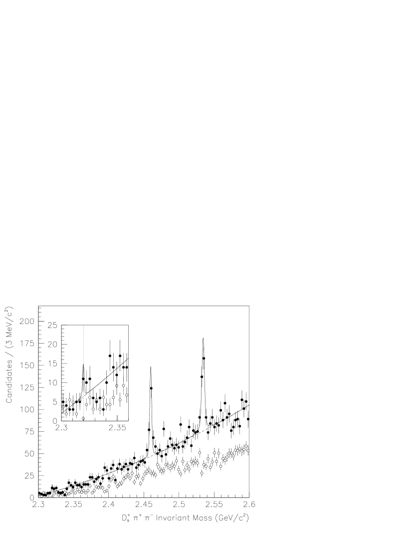
Figure 33: The invariant mass distribution of (solid points) $D^{+}_{s}\pi^{+}\pi^{-}$ candidates and (open points) the equivalent using the $D^{+}_{s}$ sidebands. The curve is the fit described in the text. The insert focuses on the low mass region. The dotted line in the insert indicates the $D_{sJ}^{*}(2317)^{+}$ mass.

Figure 34: The invariant mass distributions of MC samples of (a) $D_{sJ}(2460)^{+}$ and (b) $D_{s1}(2536)^{+}$ decay to $D^{+}_{s}\pi^{+}\pi^{-}$. The curves are the functions described in the text.

The result of the likelihood fit is shown in Fig. 33. A $D_{sJ}(2460)^{+}$ mass of $(2459.7\pm 0.2)$ ${\mathrm{\,Me\kern-1.00006ptV\!/}c^{2}}$ and $D_{s1}(2536)^{+}$ mass of $(2534.3\pm 0.3)$ ${\mathrm{\,Me\kern-1.00006ptV\!/}c^{2}}$  are obtained from raw yields of $123\pm 15$ and $193\pm 22$, respectively (statistical errors only). A raw $D_{sJ}^{*}(2317)^{+}$ yield of $6\pm 3$ is also obtained, consistent with zero.

The uncertainties in the $D_{sJ}(2460)^{+}$ and $D_{s1}(2536)^{+}$ masses are summarized in Table 7. The largest uncertainty (0.6 ${\mathrm{\,Me\kern-1.00006ptV\!/}c^{2}}$) is in the assumed $D^{+}_{s}$ mass. In comparison, uncertainties associated with the likelihood fit, such as the background shape or mass resolution, are relatively small. The remaining uncertainties are attributed to potential momentum biases in the tracking detectors.

Table 7: A summary of systematic uncertainties for the $D_{sJ}(2460)^{+}$ and $D_{s1}(2536)^{+}$ masses from the analysis of the $D^{+}_{s}\pi^{+}\pi^{-}$ final state.

	Mass Uncertainty (${\mathrm{\,Me\kern-1.00006ptV\!/}c^{2}}$)
Source	$D_{sJ}(2460)^{+}$	$D_{s1}(2536)^{+}$
$D^{+}_{s}$ mass	0.60	0.60
Signal line shape	0.03	0.01
Background function	0.01	0.01
Solenoid field	0.05	0.08
Magnetization	0.02	$<0.01$
Energy-loss correction	0.52	0.30
$\phi$ dependence	0.01	0.01
Quadrature Sum	0.80	0.68

Uncertainties in tracking have several sources, discussed in detail as part of a recent measurement of the $\Lambda_{c}$ mass from this collaboration Aubert et al. (2005). A similar treatment of these uncertainties is reproduced for this analysis. The magnetic field of the BABAR  detector is known to high precision, and variations of both the overall strength of the solenoidal field and of magnetization effects of PEP-II  beam elements produce no significant variation in measured $D^{+}_{s}\pi^{+}\pi^{-}$ mass. Residual $\phi$-dependent momentum tracking biases are also insignificant. The largest uncertainty arises from material inside the tracking volume and the effect of this material on energy loss corrections. Studies of large samples of $\Lambda$ and $K_{S}$ decays suggest that either the amount of material and/or atomic weight composition of the SVT is underestimated by approximately 20%. MC studies are used to estimate the bias introduced by this underestimation. A correction of $0.46$ ${\mathrm{\,Me\kern-1.00006ptV\!/}c^{2}}$  and $0.29$ ${\mathrm{\,Me\kern-1.00006ptV\!/}c^{2}}$  for the $D_{sJ}(2460)^{+}$ and $D_{s1}(2536)^{+}$ masses is calculated based on these studies. The final results are:

$$\begin{array}[]{lcl@{}r@{\:}c@{\:}r@{\:}c@{\:}r@{}l}m(D_{sJ}(2460)^{+})&=&(&2460.2\>&\pm\hfil\>&0.2\>&\pm\hfil\>&0.8&)\;\text{${\mathrm{\,Me\kern-1.00006ptV\!/}c^{2}}$}\\ m(D_{s1}(2536)^{+})&=&(&2534.6\>&\pm\hfil\>&0.3\>&\pm\hfil\>&0.7&)\;\text{${\mathrm{\,Me\kern-1.00006ptV\!/}c^{2}}$},\end{array}$$

where the first error is statistical and the second is systematic.

The $D_{sJ}(2460)^{+}$ and $D_{s1}(2536)^{+}$ signal PDF used in the likelihood fit of Fig. 19 was based on intrinsic widths of $\Gamma=0.1$ $\mathrm{\,Me\kern-1.00006ptV}$. After applying the same likelihood-integration technique described in Section IX for the $D^{+}_{s}\pi^{0}$ final state, and after considering systematic uncertainties in the background shape and mass reconstruction resolution, the result is a 95% CL limit of $\Gamma<3.5$ $\mathrm{\,Me\kern-1.00006ptV}$ and $\Gamma<2.5$ $\mathrm{\,Me\kern-1.00006ptV}$  for the $D_{sJ}(2460)^{+}$ and $D_{s1}(2536)^{+}$ mesons.

To estimate a total $D_{sJ}^{*}(2317)^{+}$ yield, a weight inversely proportional to the $p^{*}$-dependent $D_{sJ}^{*}(2317)^{+}$ selection efficiency is applied to each $D^{+}_{s}\pi^{+}\pi^{-}$ combination and the likelihood fit repeated. A similar process is used for the $D_{sJ}(2460)^{+}$ and $D_{s1}(2536)^{+}$ yields. The results are yields of $60\pm 40$, $760\pm 110$, and $1210\pm 160$ for the $D_{sJ}^{*}(2317)^{+}$, $D_{sJ}(2460)^{+}$, and $D_{s1}(2536)^{+}$ mesons, respectively, and for $p^{*}>3.2$ ${\mathrm{\,Ge\kern-1.00006ptV\!/}c}$ (statistical errors only).

The systematic uncertainties in the $D_{sJ}(2460)^{+}$ and $D_{s1}(2536)^{+}$ yields are summarized in Table 8. The cross section results are:

$$\begin{array}[]{lcl@{}r@{\:}c@{\:}r@{\:}c@{\:}r@{}l}\bar{\sigma}(D_{sJ}^{*}(2317)^{+}\to D^{+}_{s}\pi^{+}\pi^{-})&=&(&0.3\>&\pm\hfil\>&0.2\>&\pm\hfil\>&0.0&)\;\text{fb}\\ \bar{\sigma}(D_{sJ}(2460)^{+}\to D^{+}_{s}\pi^{+}\pi^{-})&=&(&3.3\>&\pm\hfil\>&0.5\>&\pm\hfil\>&0.3&)\;\text{fb},\\ \bar{\sigma}(D_{s1}(2536)^{+}\to D^{+}_{s}\pi^{+}\pi^{-})&=&(&5.2\>&\pm\hfil\>&0.7\>&\pm\hfil\>&0.4&)\;\text{fb},\end{array}$$

where the first error is statistical and the second is systematic.

Table 8: A summary of systematic uncertainties for the $D_{sJ}(2460)^{+}$ and $D_{s1}(2536)^{+}$ yields from the analysis of the $D^{+}_{s}\pi^{+}\pi^{-}$ final state.

	Relative Yield (%)
Source	$D_{sJ}(2460)^{+}$	$D_{s1}(2536)^{+}$
Tracking Efficiency	2.7	2.7
Signal line shape	2.7	0.3
Background function	6.1	5.6
$D^{+}_{s}$ efficiency	3.9	3.9
$D^{+}_{s}\to\phi\pi^{+}$ yield	3.9	3.9
Quadrature Sum	9.1	8.3

XVI Combined Mass and Width Results

The mass and width results for the $D_{sJ}^{*}(2317)^{+}$, $D_{sJ}(2460)^{+}$, and $D_{s1}(2536)^{+}$ mesons are summarized in Table 9. The $D_{sJ}^{*}(2317)^{+}$ and $D_{s1}(2536)^{+}$ mesons are observed in only one decay mode covered by this analysis; those portions of this table are copied unchanged from the respective sections of this paper. The $D_{sJ}(2460)^{+}$ mass is the average of that obtained from the $D^{+}_{s}\gamma$, $D^{+}_{s}\pi^{0}\gamma$, and $D^{+}_{s}\pi^{+}\pi^{-}$ final states, although the latter measurement dominates in the average due to superior systematic uncertainties. This average is calculated using a $\chi^{2}$ method that properly accounts for correlations among the systematic uncertainties in the three measurements. The limit on the intrinsic $D_{sJ}(2460)^{+}$ width $\Gamma$ is taken as the best limit obtained from these three decay modes.

Table 9: A summary of the combined mass and width results. For the masses, the first quoted uncertainty is statistical and the second is systematic. The limits on the intrinsic width $\Gamma$ are at 95% CL.

Particle	Mass (${\mathrm{\,Me\kern-1.00006ptV\!/}c^{2}}$)			$\Gamma$ ($\mathrm{\,Me\kern-1.00006ptV}$)
$D_{sJ}^{*}(2317)^{+}$	2319.6$\>\pm\>$	0.2$\>\pm\>$	1.4	$<3.8$
$D_{sJ}(2460)^{+}$	2460.1$\>\pm\>$	0.2$\>\pm\>$	0.8	$<3.5$
$D_{s1}(2536)^{+}$	2534.6$\>\pm\>$	0.3$\>\pm\>$	0.7	$<2.5$

XVII Yields and Branching Ratios

The eighteen decay yields $\bar{\sigma}$ measured in this paper are collected in Table 10. As described by Eq. 10, these numbers correspond to total yields for the decay of mesons having a center-of-mass momentum $p^{*}$ of at least 3.2 ${\mathrm{\,Ge\kern-1.00006ptV\!/}c}$  to a final state that includes a $D^{+}_{s}$ meson that decayed to $\phi\pi^{+}$.

Table 10: A summary of yield results. All cross sections are calculated for $p^{*}>3.2$ ${\mathrm{\,Ge\kern-1.00006ptV\!/}c}$. The first quoted uncertainty for the central value is statistical and the second is systematic. The limits correspond to 95% CL.

Decay Mode		Central Value (fb)			Limit (fb)
$\sigma(D_{sJ}^{*}(2317)^{+})\mathcal{B}(D_{sJ}^{*}(2317)^{+}\to X)\mathcal{B}(D^{+}_{s}\to\phi\pi^{+})$
	$D^{+}_{s}\pi^{0}$	$115.8$$\>\pm\>$	$2.9$$\>\pm\>$	$8.7$	—
	$D^{+}_{s}\gamma$	$-2.4$$\>\pm\>$	$2.3$$\>\pm\>$	$8.9$	$<15.7$
	$D^{+}_{s}\pi^{0}\pi^{0}$	$8.7$$\>\pm\>$	$6.9$$\>\pm\>$	$5.0$	$<29.0$
	$D^{+}_{s}\gamma\gamma$	$7.4$$\>\pm\>$	$4.5$$\>\pm\>$	$2.2$	$<20.6$
	$D_{s}^{*}(2112)^{+}\gamma$	$-0.5$$\>\pm\>$	$3.2$$\>\pm\>$	$8.1$	$<16.7$
	$D^{+}_{s}\pi^{+}\pi^{-}$	$0.3$$\>\pm\>$	$0.2$$\>\pm\>$	$0.0$	$<0.6$
$\sigma(D_{sJ}(2460)^{+})\mathcal{B}(D_{sJ}(2460)^{+}\to X)\mathcal{B}(D^{+}_{s}\to\phi\pi^{+})$
	$D^{+}_{s}\pi^{0}$	$-1.0$$\>\pm\>$	$1.4$$\>\pm\>$	$0.1$	$<1.7$
	$D^{+}_{s}\gamma$	$14.4$$\>\pm\>$	$1.0$$\>\pm\>$	$1.4$	—
	$D^{+}_{s}\pi^{0}\gamma$ [a]	$42.7$$\>\pm\>$	$3.5$$\>\pm\>$	$4.2$	—
	$D_{s}^{*}(2112)^{+}\pi^{0}$	$41.6$$\>\pm\>$	$5.1$$\>\pm\>$	$5.0$	—
	$D_{sJ}^{*}(2317)^{+}\gamma$	$1.1$$\>\pm\>$	$5.1$$\>\pm\>$	$5.0$	$<15.2$
	$D^{+}_{s}\pi^{0}\pi^{0}$	$5.5$$\>\pm\>$	$5.4$$\>\pm\>$	$2.4$	$<28.5$
	$D^{+}_{s}\gamma\gamma$	$3.5$$\>\pm\>$	$4.3$$\>\pm\>$	$1.7$	$<13.2$
	$D_{s}^{*}(2112)^{+}\gamma$	$-0.9$$\>\pm\>$	$3.5$$\>\pm\>$	$4.1$	$<9.7$
	$D^{+}_{s}\pi^{+}\pi^{-}$	$3.3$$\>\pm\>$	$0.5$$\>\pm\>$	$0.3$	—
$\sigma(D_{sJ}^{*}(2317)^{++})\mathcal{B}(D_{sJ}^{*}(2317)^{++}\to X)\mathcal{B}(D^{+}_{s}\to\phi\pi^{+})$
	$D^{+}_{s}\pi^{+}$	—			$<1.5$
$\sigma(D_{sJ}^{*}(2317)^{0})\mathcal{B}(D_{sJ}^{*}(2317)^{0}\to X)\mathcal{B}(D^{+}_{s}\to\phi\pi^{+})$
	$D^{+}_{s}\pi^{-}$	—			$<2.0$
$\sigma(D_{s1}(2536)^{+})\mathcal{B}(D_{s1}(2536)^{+}\to X)\mathcal{B}(D^{+}_{s}\to\phi\pi^{+})$
	$D^{+}_{s}\pi^{+}\pi^{-}$	$5.2$$\>\pm\>$	$0.7$$\>\pm\>$	$0.4$	—

[a] Includes both $D_{s}^{*}(2112)^{+}\pi^{0}$ and $D_{sJ}^{*}(2317)^{+}\gamma$ channels.

A 95% CL upper limit is calculated for those yields which are not statistically significant. These limits are calculated using a frequentist approach by determining in each case the hypothetical value of $\bar{\sigma}$ that is 1.96 standard deviations above the measured values. In order to calculate the systematic uncertainty associated with a hypothetical value of $\bar{\sigma}$, those uncertainties that are proportional to the signal yield (such as uncertainties related to selection efficiency) are scaled as appropriate. The results are shown in Table 10.

The yields listed in Table 10 are used to calculate the branching ratios shown in Table 11. For the $D_{sJ}^{*}(2317)^{+}$ meson, only one decay mode has been observed; this is used as the denominator when calculating the $D_{sJ}^{*}(2317)^{+}$ branching ratios. For the $D_{sJ}(2460)^{+}$ meson, the $D^{+}_{s}\pi^{0}\gamma$ decay mode (consisting of possible decay through either $D_{s}^{*}(2112)^{+}\pi^{0}$ or $D_{sJ}^{*}(2317)^{+}\gamma$) is chosen for this role. For completeness, the yield from hypothetical $D_{sJ}^{*}(2317)^{++}\to D^{+}_{s}\pi^{+}$ and $D_{sJ}^{*}(2317)^{0}\to D^{+}_{s}\pi^{-}$ decays is compared to $D_{sJ}^{*}(2317)^{+}\to D^{+}_{s}\pi^{0}$ decay to produce a quantity that is proportional to both the respective branching ratios and production rates.

Table 11: A summary of branching-ratio results. The first quoted uncertainty for the central value is statistical and the second is systematic. The limits correspond to 95% CL. For the hypothetical $D_{sJ}^{*}(2317)^{++}$ and $D_{sJ}^{*}(2317)^{0}$ mesons, an unknown additional factor from the ratio of production cross sections is involved. A lower limit is quoted for the $D_{sJ}(2460)^{+}\to D_{s}^{*}(2112)^{+}\pi^{0}$ results.

Decay Mode		Central Value			Limit
$\mathcal{B}(D_{sJ}^{*}(2317)^{+}\to X)/\mathcal{B}(D_{sJ}^{*}(2317)^{+}\to D^{+}_{s}\pi^{0})$
	$D^{+}_{s}\gamma$	$-0.02$$\>\pm\>$	$0.02$$\>\pm\>$	$0.08$	$<0.14$
	$D^{+}_{s}\pi^{0}\pi^{0}$	$0.08$$\>\pm\>$	$0.06$$\>\pm\>$	$0.04$	$<0.25$
	$D^{+}_{s}\gamma\gamma$	$0.06$$\>\pm\>$	$0.04$$\>\pm\>$	$0.02$	$<0.18$
	$D_{s}^{*}(2112)^{+}\gamma$	$0.00$$\>\pm\>$	$0.03$$\>\pm\>$	$0.07$	$<0.16$
	$D^{+}_{s}\pi^{+}\pi^{-}$	$0.0023$$\>\pm\>$	$0.0013$$\>\pm\>$	$0.0002$	$<0.0050$
$\mathcal{B}(D_{sJ}(2460)^{+}\to X)/\mathcal{B}(D_{sJ}(2460)^{+}\to D^{+}_{s}\pi^{0}\gamma)$ [a]
	$D^{+}_{s}\pi^{0}$	$-0.023$$\>\pm\>$	$0.032$$\>\pm\>$	$0.005$	$<0.042$
	$D^{+}_{s}\gamma$	$0.337$$\>\pm\>$	$0.036$$\>\pm\>$	$0.038$	—
	$D_{s}^{*}(2112)^{+}\pi^{0}$	$0.97$$\>\pm\>$	$0.09$$\>\pm\>$	$0.05$	$>0.75$
	$D_{sJ}^{*}(2317)^{+}\gamma$	$0.03$$\>\pm\>$	$0.09$$\>\pm\>$	$0.05$	$<0.25$
	$D^{+}_{s}\pi^{0}\pi^{0}$	$0.13$$\>\pm\>$	$0.13$$\>\pm\>$	$0.06$	$<0.68$
	$D^{+}_{s}\gamma\gamma$	$0.08$$\>\pm\>$	$0.10$$\>\pm\>$	$0.04$	$<0.33$
	$D_{s}^{*}(2112)^{+}\gamma$	$-0.02$$\>\pm\>$	$0.08$$\>\pm\>$	$0.10$	$<0.24$
	$D^{+}_{s}\pi^{+}\pi^{-}$	$0.077$$\>\pm\>$	$0.013$$\>\pm\>$	$0.008$	—
$\sigma(D_{sJ}^{*}(2317)^{++})/\sigma(D_{sJ}^{*}(2317)^{+})\times$
$\mathcal{B}(D_{sJ}^{*}(2317)^{++}\to X)/\mathcal{B}(D_{sJ}^{*}(2317)^{+}\to D^{+}_{s}\pi^{0})$
	$D^{+}_{s}\pi^{+}$	—			$<0.017$
$\sigma(D_{sJ}^{*}(2317)^{0})/\sigma(D_{sJ}^{*}(2317)^{+})\times$
$\mathcal{B}(D_{sJ}^{*}(2317)^{0}\to X)/\mathcal{B}(D_{sJ}^{*}(2317)^{+}\to D^{+}_{s}\pi^{0})$
	$D^{+}_{s}\pi^{-}$	—			$<0.013$

[a] Denominator includes both $D_{s}^{*}(2112)^{+}\pi^{0}$ and $D_{sJ}^{*}(2317)^{+}\gamma$ channels.

In order to calculate the systematic uncertainty in the branching ratio results, systematic uncertainties common to the nominator and denominator are first discarded. Such common uncertainties include those associated with the $D^{+}_{s}\to\phi\pi^{+}$ branching ratio correction and, in some cases, those associated with $\pi^{0}$ and $\gamma$ reconstruction efficiency.

A 95% CL upper limit is calculated for those branching ratios associated with decay modes that lack statistical signficance. The method used is similar to the frequentist recipe used for the upper limits on the cross section. The results are included in Table 11.

XVIII Discussion

The results in this paper confirm previous measurements, with generally higher precision. No new decay modes have been uncovered. Lacking any additional evidence to the contrary, the $J^{P}=0^{+}$ and $J^{P}=1^{+}$ assignments for the $D_{sJ}^{*}(2317)^{+}$ and $D_{sJ}(2460)^{+}$ mesons remain a viable hypothesis. Except, perhaps, for the mass, there is currently no conflict with the interpretation of the $D_{sJ}^{*}(2317)^{+}$ and $D_{sJ}(2460)^{+}$ mesons as the $J^{P}=0^{+}$ and $J^{P}=1^{+}$ $p$-wave $c\bar{s}$ states, as shown in Fig. 1.

The $D_{sJ}(2460)^{+}$ meson mass measured in this analysis is an improvement over previous measurements Besson et al. (2003); Aubert et al. (2004a); Abe et al. (2004). High precision is obtained by using a decay mode that includes only charged particles coupled with a detailed understanding of the performance of the BABAR  tracking detectors. The determination of the $D_{sJ}^{*}(2317)^{+}$ mass remains limited by uncertainties in EMC energy scale.

No intrinsic width of any statistical signficance is observed for either the $D_{sJ}^{*}(2317)^{+}$ or $D_{sJ}(2460)^{+}$ meson. There is sufficient detector resolution in the $D^{+}_{s}\pi^{+}\pi^{-}$ decay mode that better limits for the $D_{sJ}(2460)^{+}$ meson should be attainable in the future with higher statistics. In contrast, limits on the $D_{sJ}^{*}(2317)^{+}$ width are currently limited by systematic uncertainties and will be difficult to improve.

Both the mass and width results for the $D_{s1}(2536)^{+}$ meson obtained from the decay to $D^{+}_{s}\pi^{+}\pi^{-}$ are consistent with prior measurements Eidelman et al. (2004) and theoretical expectations Godfrey and Isgur (1985); Godfrey and Kokoski (1991); Isgur and Wise (1991); Di Pierro and Eichten (2001).

The analysis of the decay $D_{sJ}(2460)^{+}\to D_{s}^{*}(2112)^{+}\pi^{0}$ is complicated by the overlap in kinematics of the hypothetical decay $D_{sJ}(2460)^{+}\to D_{sJ}^{*}(2317)^{+}\gamma$. The analysis presented here applies a likelihood technique to separate these two decay modes and provide a limit on the latter. A previous analysis from BELLE Abe et al. (2004) of the decay $D_{sJ}(2460)^{+}\to D_{s}^{*}(2112)^{+}\pi^{0}$ did not account for such possible contamination. As a consequence, it should be noted, their quoted yield for the decay $D_{sJ}(2460)^{+}\to D_{s}^{*}(2112)^{+}\pi^{0}$ should be compared to the $D_{sJ}(2460)^{+}\to D^{+}_{s}\pi^{0}\gamma$ result presented here in which both decay channels ($D_{sJ}^{*}(2317)^{+}\gamma$ and $D_{s}^{*}(2112)^{+}\pi^{0}$) are included together. Specifically, the BELLE measurement of the branching fraction from $e^{+}e^{-}\to c\overline{c}$ production is $\mathcal{B}(D_{sJ}(2460)^{+}\to D^{+}_{s}\gamma)/\mathcal{B}(D_{sJ}(2460)^{+}\to D_{s}^{*}(2112)^{+}\pi^{0})=0.55\pm 0.13\;(\text{stat.})\pm 0.08\;(\text{syst.})$ and can be compared directly to the result of this analysis ($0.337\pm 0.036\;(\text{stat.})\pm 0.038\;(\text{syst.})$). The less precise BELLE result is somewhat larger, but still compatible within uncertainties. The result presented here is consistent with BELLE ($0.38\pm 0.11\;(\text{stat.})\pm 0.04\;(\text{syst.})$) Krokovny et al. (2003) and BABAR  ($0.275\pm 0.045\;(\text{stat.})\pm 0.020\;(\text{syst.})$) Aubert et al. (2004b) measurements from $D_{sJ}(2460)^{+}$ production in $B$ decay.

The remaining branching ratio results shown in Table 11 are generally competitive with the corresponding BELLE limits Abe et al. (2004). An exception is the limit on the decay $D_{sJ}^{*}(2317)^{+}\to D^{+}_{s}\gamma$. The BELLE publication, however, does not address the difficulties associated with modeling the $D_{sJ}^{*}(2317)^{+}\to D^{+}_{s}\pi^{0}$ reflection (see Fig. 14) which is the source of much of the systematic uncertainty quoted in this analysis.

The searches for the $D^{+}_{s}\pi^{0}\pi^{0}$ and $D^{+}_{s}\gamma\gamma$ decay modes of the $D_{sJ}^{*}(2317)^{+}$ and $D_{sJ}(2460)^{+}$ have been reported in this analysis for the first time. Both final states suffer from large backgrounds. More precise information on these modes will require more advanced analysis techniques, perhaps with the use of $B$ meson decay or some other method of background suppression.

The $D_{sJ}^{*}(2317)^{+}$ and $D_{sJ}(2460)^{+}$ masses are considerably lower than predictions from potential models developed before their discovery. Since the $D_{sJ}^{*}(2317)^{+}$/$D_{sJ}(2460)^{+}$ mass splitting is so much larger than that for the $D_{s1}(2536)^{+}$ and $D_{s2}(2573)^{+}$ mesons, it would appear that this conflict is intrinsic. Studies from Cahn and Jackson Cahn and Jackson (2003) suggest, however, that it is possible with some adjustment to fit the $D_{sJ}^{*}(2317)^{+}$ and $D_{sJ}(2460)^{+}$ into a perturbative model. In any case, given the approximate nature of these models, there is a danger that even large discrepancies can be overstated.

In contrast, according to Bardeen, Eichten, and Hill, models based on chiral symmetry naturally accommodate the large $D_{sJ}^{*}(2317)^{+}$/$D_{sJ}(2460)^{+}$ mass splitting Bardeen et al. (2003) when the $D_{sJ}^{*}(2317)^{+}$ and $D_{sJ}(2460)^{+}$ multiplet is treated as a chiral partner of the ground state $D^{+}_{s}$ and $D_{s}^{*}(2112)^{+}$ mesons. Their model provides specific predictions for branching ratios, notably $\mathcal{B}(D_{sJ}(2460)^{+}\to D^{+}_{s}\pi^{+}\pi^{-})/\mathcal{B}(D_{sJ}(2460)^{+}\to D_{s}^{*}(2112)^{+}\pi^{0})\approx 0.09$ and $\mathcal{B}(D_{sJ}(2460)^{+}\to D^{+}_{s}\gamma)/\mathcal{B}(D_{sJ}(2460)^{+}\to D_{s}^{*}(2112)^{+}\pi^{0})\approx 0.24$, both in good agreement with our measurements of ($0.077\pm 0.015$) and ($0.337\pm 0.052$), respectively. Other branching ratio predictions are $\mathcal{B}(D_{sJ}^{*}(2317)^{+}\to D_{s}^{*}(2112)^{+}\gamma)/\mathcal{B}(D_{sJ}^{*}(2317)^{+}\to D^{+}_{s}\pi^{0})\approx 0.08$ and $\mathcal{B}(D_{sJ}(2460)^{+}\to D_{sJ}^{*}(2317)^{+}\gamma)/\mathcal{B}(D_{sJ}(2460)^{+}\to D_{s}^{*}(2112)^{+}\pi^{0})\approx 0.13$. Neither decay is observed by this analysis, but the corresponding upper limits still exceed the predicted branching ratios. This model also predicts a total intrinsic width of 23.2 $\mathrm{\,ke\kern-1.00006ptV}$  and 38.2 $\mathrm{\,ke\kern-1.00006ptV}$  for the $D_{sJ}^{*}(2317)^{+}$ and $D_{sJ}(2460)^{+}$ mesons, respectively, far below the limits measured here.

Perturbative calculations from Godfrey Godfrey (2003) predict branching ratios of $0.19$ and $0.55$ for the radiative transition decay of the $D_{sJ}^{*}(2317)^{+}$ and $D_{sJ}(2460)^{+}$ to $D_{s}^{*}(2112)^{+}\gamma$. These predictions are not consistent with the results reported here. This discrepancy could be considered evidence that both the $D_{sJ}^{*}(2317)^{+}$ and $D_{sJ}(2460)^{+}$ are not $c\bar{s}$ mesons. These theoretical predictions, however, are plagued with large uncertainties in the partial widths of the isospin-violating $D_{sJ}^{*}(2317)^{+}\to D^{+}_{s}\pi^{0}$ and $D_{sJ}(2460)^{+}\to D_{s}^{*}(2112)^{+}\pi^{0}$ decays. In addition, leading-order corrections to the radiative transition partial rates might explain current experimental limits Mehen and Springer (2004). Nevertheless, the possibility that the $D_{sJ}^{*}(2317)^{+}$ and $D_{sJ}(2460)^{+}$ are some type of new bound state, such as a four-quark $DK$ molecule, should be taken seriously.

The possibility of four-quark states has long been proposed Jaffe (1977); Lipkin (1977). Perhaps the most unambiguous signature of the molecular interpretation of the $D_{sJ}^{*}(2317)^{+}$ meson would be the production of neutral and charged partners decaying to $D^{+}_{s}\pi^{\pm}$. For an isospin 1 $DK$ molecule, production of these isospin partners is expected at the same rate as the $D_{sJ}^{*}(2317)^{+}$ Barnes et al. (2003). This is clearly ruled out by our data. Other molecular interpretations, however, do not have this limitation Barnes et al. (2003); Lipkin (2004), and it may be challenging to rule them all out with the data from the $B$-factories alone.

Finally, now that more precise data on the $D_{sJ}^{*}(2317)^{+}$ and $D_{sJ}(2460)^{+}$ is available, measurements of the other $c\bar{s}$ states have become more important. The measurement of the $D_{s1}(2536)^{+}$ mass in this analysis will be helpful in further constraining models. With high statistics samples available from both $B$-factory experiments, improvements in the parameters of the $D^{+}_{s}$, $D_{s}^{*}(2112)^{+}$, and $D_{s2}(2573)^{+}$ mesons should not be neglected and will hopefully follow soon.

XIX Conclusion

An updated analysis of the $D_{sJ}^{*}(2317)^{+}$ and $D_{sJ}(2460)^{+}$ mesons using 232 ${\rm fb}^{-1}$ of $e^{+}e^{-}\to c\bar{c}$ data is performed. Established signals from the decay $D_{sJ}^{*}(2317)^{+}\to D^{+}_{s}\pi^{0}$ and $D_{sJ}(2460)^{+}\to D^{+}_{s}\pi^{0}\gamma$, $D^{+}_{s}\gamma$, and $D^{+}_{s}\pi^{+}\pi^{-}$ are confirmed. A detailed analysis of invariant mass distributions of these final states including consideration of the background introduced by reflections of other $c\bar{s}$ decays produces the following mass values:

$$\begin{array}[]{lcl@{}r@{\:}c@{\:}r@{\:}c@{\:}r@{}l}m(D_{sJ}^{*}(2317)^{+})&=&(&2319.6\>&\pm\hfil\>&0.2\>&\pm\hfil\>&1.4&)\;{\mathrm{\,Me\kern-1.00006ptV\!/}c^{2}}\\ m(D_{sJ}(2460)^{+})&=&(&2460.1\>&\pm\hfil\>&0.2\>&\pm\hfil\>&0.8&)\;{\mathrm{\,Me\kern-1.00006ptV\!/}c^{2}},\end{array}$$

where the first error is statistical and the second systematic. Upper 95% CL limits of $\Gamma<3.8$ $\mathrm{\,Me\kern-1.00006ptV}$  and $\Gamma<3.5$ $\mathrm{\,Me\kern-1.00006ptV}$  are calculated for the intrinsic $D_{sJ}^{*}(2317)^{+}$ and $D_{sJ}(2460)^{+}$ widths. All results are consistent with previous measurements.

The following final states are investigated: $D^{+}_{s}\pi^{0}$, $D^{+}_{s}\gamma$, $D_{s}^{*}(2112)^{+}\pi^{0}$, $D_{sJ}^{*}(2317)^{+}\gamma$, $D^{+}_{s}\pi^{0}\pi^{0}$, $D_{s}^{*}(2112)^{+}\gamma$, $D^{+}_{s}\gamma\gamma$, $D^{+}_{s}\pi^{\pm}$, and $D^{+}_{s}\pi^{+}\pi^{-}$. No statistically significant evidence of new decay modes is observed. The following branching ratios are measured:

$$\begin{array}[]{ccl@{}r@{\:}c@{\:}r@{\:}c@{\:}r}\frac{\mathcal{B}(D_{sJ}(2460)^{+}\to D^{+}_{s}\gamma)}{\mathcal{B}(D_{sJ}(2460)^{+}\to D^{+}_{s}\pi^{0}\gamma)}&=&&0.337\>&\pm\hfil\>&0.036\>&\pm\hfil\>&0.038\\ \frac{\mathcal{B}(D_{sJ}(2460)^{+}\to D^{+}_{s}\pi^{+}\pi^{-})}{\mathcal{B}(D_{sJ}(2460)^{+}\to D^{+}_{s}\pi^{0}\gamma)}&=&&0.077\>&\pm\hfil\>&0.013\>&\pm\hfil\>&0.008\end{array}$$

where the first error is statistical and the second systematic. The data are consistent with the decay $D_{sJ}(2460)^{+}\to D^{+}_{s}\pi^{0}\gamma$ proceeding entirely through $D_{s}^{*}(2112)^{+}\pi^{0}$.

Since the results presented here are consistent with $J^{P}=0^{+}$ and $J^{P}=1^{+}$ spin-parity assignments for the $D_{sJ}^{*}(2317)^{+}$ and $D_{sJ}(2460)^{+}$ mesons, these two states remain viable candidates for the lowest lying $p$-wave $c\bar{s}$ mesons. The lack of evidence for some radiative decays, in particular $D_{sJ}^{*}(2317)^{+}\to D_{s}^{*}(2112)^{+}\gamma$ and $D_{sJ}(2460)^{+}\to D_{s}^{*}(2112)^{+}\gamma$, are in contradiction with this hypothesis according to some calculations, but large theoretical uncertainties remain. No state near the $D_{sJ}^{*}(2317)^{+}$ mass is observed decaying to $D^{+}_{s}\pi^{\pm}$. If charged or neutral partners to the $D_{sJ}^{*}(2317)^{+}$ exist (as would be expected if the $D_{sJ}^{*}(2317)^{+}$ is a four-quark state), some mechanism is required to suppress their production in $e^{+}e^{-}$ collisions.

References

Aubert et al. (2003)
B. Aubert et al.
(BABAR), Phys. Rev. Lett.
90, 242001
(2003).
Besson et al. (2003)
D. Besson et al.
(CLEO), Phys. Rev.
D68, 032002
(2003).
Abe et al. (2004)
K. Abe et al.
(BELLE), Phys. Rev. Lett.
92, 012002
(2004).
Aubert et al. (2004a)
B. Aubert et al.
(BABAR), Phys. Rev.
D69, 031101
(2004a).
Godfrey and Isgur (1985)
S. Godfrey and
N. Isgur,
Phys. Rev. D32,
189 (1985).
Godfrey and Kokoski (1991)
S. Godfrey and
R. Kokoski,
Phys. Rev. D43,
1679 (1991).
Isgur and Wise (1991)
N. Isgur and
M. B. Wise,
Phys. Rev. Lett. 66,
1130 (1991).
Di Pierro and Eichten (2001)
M. Di Pierro and
E. Eichten,
Phys. Rev. D64,
114004 (2001).
Barnes et al. (2003)
T. Barnes,
F. E. Close, and
H. J. Lipkin,
Phys. Rev. D68,
054006 (2003).
Lipkin (2004)
H. J. Lipkin,
Phys. Lett. B580,
50 (2004).
(11)
Inclusion of charge conjugate states is implied throughout this
paper.
Krokovny et al. (2003)
P. Krokovny et al.
(BELLE), Phys. Rev. Lett.
91, 262002
(2003).
Aubert et al. (2004b)
B. Aubert et al.
(BABAR), Phys. Rev. Lett.
93, 181801
(2004b).
Aubert et al. (2002)
B. Aubert et al.
(BABAR), Nucl. Instr. Meth.
A479, 1 (2002).
Eidelman et al. (2004)
S. Eidelman et al.
(Particle Data Group), Phys.
Lett. B592, 1
(2004).
Aubert et al. (2005)
B. Aubert et al.
(BABAR), Phys. Rev.
D72, 052006
(2005).
Cahn and Jackson (2003)
R. N. Cahn and
J. D. Jackson,
Phys. Rev. D68,
037502 (2003).
Bardeen et al. (2003)
W. A. Bardeen,
E. J. Eichten,
and C. T. Hill,
Phys. Rev. D68,
054024 (2003).
Godfrey (2003)
S. Godfrey,
Phys. Lett. B568,
254 (2003).
Mehen and Springer (2004)
T. Mehen and
R. P. Springer,
Phys. Rev. D70,
074014 (2004).
Jaffe (1977)
R. L. Jaffe,
Phys. Rev. D15,
281 (1977).
Lipkin (1977)
H. J. Lipkin,
Phys. Lett. B70,
113 (1977).