A high-precision measurement
of the di-electron widths
of the Upsilon(1S), Upsilon(2S),
and Upsilon(3S) mesons
at CLEO-III

Abstract

The di-electron width of an Upsilon meson is the decay rate of the Upsilon into an electron-positron pair, expressed in units of energy. We measure the di-electron width of the Upsilon(1S) meson to be 1.354 $\pm$ 0.004 $\pm$ 0.020 keV (the first uncertainty is statistical and the second is systematic), the di-electron width of the Upsilon(2S) to be 0.619 $\pm$ 0.004 $\pm$ 0.010 keV and that of the Upsilon(3S) to be 0.446 $\pm$ 0.004 $\pm$ 0.007 keV. We determine these values with better than 2% precision by integrating the Upsilon production cross-section from electron-positron collisions over their collision energy. Our incident electrons and positrons were accelerated and collided in the Cornell Electron Storage Ring, and the Upsilon decay products were observed by the CLEO-III detector. The di-electron widths probe the wavefunctions of the Strongly-interacting bottom quarks that constitute the three Upsilon mesons, information which is especially interesting to check high-precision Lattice QCD calculations of the nuclear Strong force.

James Adam M c Cann was induced to be born on Friday, July 2, 1976, as that weekend was one that even delivery surgeons wanted to have off. His loving parents are Tom M c Cann and Donna Scott. James later married Melanie Pivarski, and in an effort to balance an overwhelming cultural practice, took her last name. Thus, he is now known as James M c Cann Pivarski, and may be the only man on earth whose middle initial is an “M c .”

James (Jim) was educated in public schools in Westfield, MA, later studied physics with a minor in mathematics at Carnegie Mellon University in Pittsburgh, PA, and finally experimental particle physics at Cornell University in Ithaca, NY. With this document, he completes his twenty-fifth year of schooling. Soon Jim and Melanie will move to College Station, TX, to do research in physics and mathematics (respectively) at Texas A&M University.

Jim was originally interested in physics as a means of mystifying his understanding of the world, rather than making it clearer, which some of the conclusions of modern physics provide for. His assumption that the universe was not what it seemed to be blended with his affinity for the existentialism of Albert Camus and his former skepticism of all experience, including subjective experience. Trying to take these views seriously, he suffered a philosophical breakdown and reconsidered his world-view at a fundamental level. Today, he begins by assuming that things are as they appear to be, modifying that assumption as observed complications arise. This is why Jim is now an experimentalist, and it is also related to his conversion to Catholicism (when applied to subjective experience, rather than objective). Before college, Jim’s aspiration was to create special effects for movies, to convince the senses of something which isn’t true. Now he does the opposite.

Chapter 1 Introduction and Motivation

1.1 The $\Upsilon$ Di-electron Width and Why it is Important

An Upsilon ($\Upsilon$) meson is a composite particle consisting of a bottom quark ($b$) and an anti-bottom quark ($\bar{b}$) bound with their spins aligned in a $J=1$ quantum mechanical wavefunction, where $J$ is the total angular momentum. This meson is a nuclear analogy of ortho-positronium in atomic physics. The di-electron width is the rate of $\Upsilon$ decay into an electron/positron pair, and measuring it provides unique experimental access to the physical size of the $b\bar{b}$ wavefunction and its total decay rate— the average extension of the $\Upsilon$ meson in both space and time.

The $b\bar{b}$ system, also known as bottomonium, is the most non-relativistic system of quarks bound by the nuclear Strong force. This is because the bottom quark is the heaviest quark that can participate in the Strong force, the top decaying immediately into bottom by the Electroweak force. Unlike much more abundant protons and neutrons, whose masses consist almost entirely of the kinetic energy of the constituent quarks and gluons, 94% of the mass of the lightest $\Upsilon$ consists of the mass of its two bottom quarks. This simplifies the dynamics of bottomonium and even permits description in terms of a potential, making it a good testing ground for Strong force calculations.

Quantum Chromodynamics (QCD) has long been accepted as the correct description of the nuclear Strong force (with possible modifications only at TeV energies and above) because of its success in predicting scattering interactions above one GeV and its qualitative explanation of low-energy phenomena like quark confinement. Today, the Lattice QCD technique, which simulates QCD on a computer, is yielding few-percent calculations of low-energy phenomena from first principles— in particular, $\Upsilon$ properties such as the di-electron widths. Precise experimental knowledge of the $\Upsilon$ di-electron widths will test the new Lattice QCD techniques that made this advance possible.

The di-electron widths check Lattice QCD in a way that is key for Electroweak physics. The CP violation parameters $V_{td}$ and $V_{ub}$, fundamental constants in the Standard Model, could be extracted from existing hadronic measurements much more precisely if the strength of the force between quarks were better known. Lattice QCD can help, but precise Lattice results will only be trusted if similar calculations can be experimentally verified. The $\Upsilon$ di-electron width closely resembles the factor that limits our knowledge of $V_{td}$, and thus will provide a cross-check that will either lend credence to or cast doubt on the $V_{td}$ extraction.

Di-electron widths of the $\Upsilon$ resonances have been measured before, but not with the precision that is now being demanded by Lattice QCD. This document represents a comprehensive study of the $\Upsilon(1S)$, $\Upsilon(2S)$, and $\Upsilon(3S)$ di-electron widths, with 50 times the data of any previous measurement. We present di-electron width measurements of the $\Upsilon(1S)$, $\Upsilon(2S)$, and $\Upsilon(3S)$ with 1.5%, 1.8%, and 1.8% total uncertainty, respectively. This is the second-ever measurement of the $\Upsilon(3S)$ di-electron width, improving its precision by a factor of five. Furthermore, measuring all three resonances in the same study permits us to derive very precise ratios of di-electron widths, where the tightest constraint on theory is likely to be. Without this measurement, comparisons with Lattice QCD would probably be limited by experiment.

1.2 The Bottomonium Potential and Mass Eigenstates

The $b$-quark and the $\bar{b}$-quark in bottomonium attract each other by the nuclear Strong force, which in QCD is mediated by gluons, the nuclear analogy of virtual photons. The two quarks are charged with opposite “colors,” in a quantum mechanical superposition of red/anti-red, blue/anti-blue, and green/anti-green states, which are constantly traded for each other by the doubly-colored gluons. (The exchange of a red/anti-green gluon will turn a red/anti-red $b\bar{b}$ system green/anti-green, for instance. See Figure 1.1(a).) Because the gluons carry color charge, they can interact with other gluons and spawn complicated networks of interactions between the two quarks (Figure 1.1(b)), which increases the interaction strength with distance. Bottom quarks are usually separated by a femtometer, and at this distance scale, the coupling constant of QCD is of order unity. Feynman diagrams with many vertices are not suppressed relative to simple diagrams, and therefore a calculation of the force between the two quarks does not submit to a perturbative expansion.

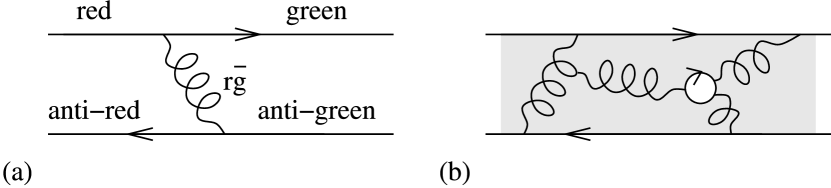
Figure 1.1: (a) An example of a gluon as a force propagator and a carrier of color charge. Directed lines are quarks and springs are gluons. (b) An exchange between two quarks involving a complicated network of gluons and a light quark/anti-quark pair. Grey shading indicates the sum of all such amplitudes.

A very successful model of the force between $b$ and $\bar{b}$ consists of a Coulomb-like potential at short distances (though about 50 times stronger) and a linear potential at large distances (which limits to a constant force of about 14 tons), as illustrated in Figure 1.2(a) [1]. At large distances, a string of self-interacting gluons, stretched between the two quarks, is responsible for the linear component. This string will generate a real quark/anti-quark pair and snap if stretched with sufficient energy. There are three $J=1$ solutions to the Schrödinger equation below this threshold: they are labeled $\Upsilon(1S)$, $\Upsilon(2S)$, and $\Upsilon(3S)$. States above this threshold have a very different pattern of decay modes and are beyond the scope of this study.

Figure 1.2: (a) Schematic of the potential energy between two quarks as a function of separation. (b) Quantitative level diagram of $J=1$ $b\bar{b}$ solutions ($\Upsilon$). The $\Upsilon(4S)$ lies just above the string-breaking threshold (dashed line).

These three mass eigenstates are the bottomonium equivalent of atomic energy levels— discrete lines of allowed mass-energies. But, just as in atomic spectra, the short lifetimes of these states imply a broadening of their spectral lines: they are not perfect time-independent solutions. The full-width of an $\Upsilon$ resonance at half-maximum, $\Gamma$, is equal to its decay rate, in analogy with excited atomic resonances. If we partition the $\Upsilon$ decays into distinguishable modes, one being $\Upsilon\to e^{+}e^{-}$, the total decay rate is a sum of those modes. Hence, $\Gamma_{ee}=\Gamma\,{\mathcal{B}}_{ee}$, where $\Gamma_{ee}$ is the di-electron width and ${\mathcal{B}}_{ee}$ is the fraction of $\Upsilon$ mesons that decay to $e^{+}e^{-}$, that is, the branching fraction to $e^{+}e^{-}$.

The $\Upsilon$ meson decays into $e^{+}e^{-}$ by $b\bar{b}$ annihilation (Figure 1.3), which is a point-like interaction. The $b$ and the $\bar{b}$ must fluctuate to the same point in space for the reaction to proceed. This probability, which is the square of the $b\bar{b}$ spatial wavefunction evaluated at the origin ($|\psi(0,0,0)|^{2}$), is therefore a factor in $\Gamma_{ee}$.

$$\Gamma_{ee}=3{Q_{b}}^{2}\,\frac{16\pi\alpha^{2}}{3}\,\frac{|\psi(0,0,0)|^{2}}{{M_{\Upsilon}}^{2}}$$ (1.1)

where $Q_{b}=1/3$, the $b$-quark electric charge, $\alpha$ is the Electromagnetic fine structure constant and $M_{\Upsilon}$ is the $\Upsilon$ mass [2]. This is a non-relativistic approximation: relativistic corrections replace the wavefunction at the origin with an integral of values very close to the origin. Because of this dependence on knowledge of the $b\bar{b}$ wavefunction, and therefore the potential, a first-principles calculation $\Gamma_{ee}$ will require non-perturbative QCD.

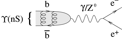
Figure 1.3: Decay diagram of $\Upsilon(nS)\to e^{+}e^{-}$. The $Z^{0}$ contribution is 0.25% of the total rate.

1.3 Lattice QCD

Feynman path integrals provide a general approach to quantum field theory that don’t rely on a perturbative expansion. In this formalism, the amplitude of a process is calculated as a weighted sum of all possible ways it can proceed. The value of every field at every point in space in the initial state is allowed to vary as an arbitrary function of time to the final state, and these paths are weighted by their action. This is a generalization of Lagrange’s method in classical physics, in which the true path is the one which minimizes action. In quantum physics, all paths which nearly minimize action contribute to the amplitude of a process (Figure 1.4(a)).

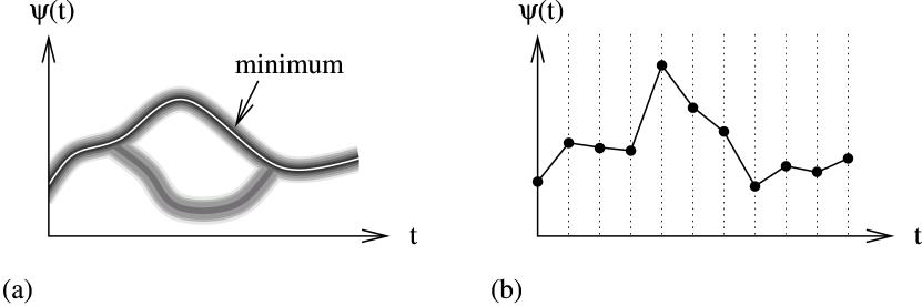
Figure 1.4: (a) Paths in field strength ($\psi$) versus time. The minimum (white) is the classical solution and the path which contributes the most to the quantum amplitude; shades of grey represent other quantum paths with smaller contributions to the total amplitude. (b) A path approximated by a discrete time sequence.

To calculate a sum over a set of arbitrary paths, one must discretize space-time into time slices and space cubes. The path of a field value in a space cube from the initial state to the final state is a sequence of values for each time slice (Figure 1.4(b)). A sequence of $N$ values is a vector in an $N$-dimensional vector space: the weighting factor is integrated over these vector spaces. To obtain a realistic result, one must afterward limit the discretization scale to zero.

In general, realistic problems like QCD, the integral will not be analytic and must be solved by numerical integration. The integral will have a fixed number of dimensions, which implies a fixed discretization of space-time that can only be lifted by extrapolating several calculations toward zero lattice size. This discretization is the lattice of Lattice QCD. Quark field values are represented on a four-dimensional lattice of space-time points with gluon field values on the edges connecting them.

This is a very computationally intensive problem, since the number of dimensions in the integral scales with the number of grid points, and one must maximize the number of grid points to extrapolate to the continuum limit. Over the past 30 years, theorists have improved the algorithms of Lattice QCD and sought approximations to make realistic calculations tractable.

The most time-consuming part of most Lattice QCD calculations is the polarization of the vacuum by light quarks. In terms of Feynman diagrams, these are interruptions of a gluon propagator by loops of $u\bar{u}$, $d\bar{d}$ and $s\bar{s}$ pairs, which can be ignored or suppressed by assuming infinite or very heavy up, down, and strange quark masses (Figure 1.5). This approximation is known as the quenched approximation, and it permits calculations with 10–20% systematic uncertainties.

Figure 1.5: Vacuum polarization by light quarks.

This situation was dramatically improved in the late 1990’s by the development of new algorithms based on the Symanzik-improved staggered-quark formalism [3]. These algorithms are by far the most efficient known, and the formalism features an exact chiral symmetry that particularly benefits simulations with small light quark masses. Realistic up and down quark masses are still out of reach, but simulations using masses three times too large can be accurately extrapolated with chiral perturbation theory. Thus, “unquenched” calculations are now possible, resulting in the accurate prediction of many masses and decay rates, as demonstrated in Figure 1.6.

Figure 1.6: Lattice QCD calculations divided by experimental measurements for nine quantities, without and with quark vacuum polarization (left and right panels, respectively). (The notation $\Upsilon(n-1S)$ refers to the mass difference between $\Upsilon(n)$ and $\Upsilon(1S)$.)

This algorithmic speed comes at a conceptual price: the staggered-quark formalism introduces four equivalent species of each quark field, called “tastes.” These are artifacts of the formalism and are unrelated to quark flavor. Each of these tastes contributes to the vacuum polarization, resulting in loop contributions which are four times too large. To correct for this, the quark determinant in the action is replaced by its fourth root, a procedure which is rigorous in the free-field theory and in perturbative QCD, but introduces violations of Lorentz symmetry at short distances in the lattice simulation. Although these non-physical effects can be removed by interpolating between the lattice points with perturbative QCD, this issue makes the new algorithms controversial, and it is one aspect that will be tested by confrontations with experiment.

The di-electron width may be determined from $\Upsilon$ simulations by extracting the $b\bar{b}$ wavefunction at the origin and applying Equation 1.1. In a path integral context, the wavefunction is the quark field amplitude. These simulations employ a non-relativistic QCD action with relativistic corrections (NRQCD), because the de Broglie wavelength of a massive $b$ quark would require impractically narrow time slices.

Simulations of the $\Upsilon$ mesons have been generated by the HPQCD collaboration, but the determination of $\Gamma_{ee}$ from them is not yet complete [4]. To properly calculate $\Gamma_{ee}$, one needs to correct the lattice wavefunction for discretization effects through a constant, $Z_{\mbox{\scriptsize match}}^{\mbox{\scriptsize vector}}$, that matches the lattice approximations of the virtual photon current to a continuum renormalization scheme. The leading term in $Z_{\mbox{\scriptsize match}}^{\mbox{\scriptsize vector}}$ is on the order of the Strong coupling constant $\alpha_{s}$, about 20%. This calculation is in progress. However, $Z_{\mbox{\scriptsize match}}^{\mbox{\scriptsize vector}}$ largely cancels in ratios of $\Gamma_{ee}$: for instance, $\Gamma_{ee}$ from the $\Upsilon(2S)$ divided by $\Gamma_{ee}$ from the $\Upsilon(1S)$ can already be extracted with a 10% uncertainty.

$$\left.\frac{\Gamma_{ee}(2S)}{\Gamma_{ee}(1S)}\right|_{\mbox{\scriptsize HPQCD}}=0.43\pm 0.04\mbox{.}$$ (1.2)

This uncertainty is primarily due to residual discretization errors, evident from the steep dependence of the result on lattice spacing size (Figure 1.7). When the discretization correction has been calculated, the uncertainty in this ratio should be only a few percent, while absolute $\Gamma_{ee}$ values should have uncertainties on the 10%-level. This is why experimentally precise ratios of $\Gamma_{ee}$ are also valuable. The ratios test the NRQCD treatment of the $b$ quarks with high precision, though they are less sensitive to the $Z_{\mbox{\scriptsize match}}^{\mbox{\scriptsize vector}}$ corrections.

Figure 1.7: HPQCD calculations of $\Gamma_{ee}(2S)/\Gamma_{ee}(1S)$ times the ratio of masses squared as a function of lattice grid size $a$. Square data points represent calculations with light quark masses close to their natural values, and triangular points are quenched (infinite light quark masses).

1.4 Relationship to Electroweak Parameter Extraction

Lattice verification of $\Gamma_{ee}$ is particularly significant for an application of the technique to Electroweak physics. Vertices in Feynman diagrams that join a top quark, a down quark, and a $W$ boson contribute an a priori unknown factor, $V_{td}$, to the amplitude (Figure 1.8). This parameter is a fundamental constant in the Standard Model and is essential for violation of charge-parity (CP) symmetry: if $V_{td}$ were zero, the Standard Model would be CP symmetric (exchanging particles for antiparticles and mirror-transforming space would preserve all observables). To determine $V_{td}$, one must resort to measurements of bound quark systems, because bare quarks do not exist in nature. The transition rates for these systems depend both on $V_{td}$ and on QCD factors related to the structure of the bound state. Lattice QCD can calculate these factors and thereby extract $V_{td}$.

Figure 1.8: The vertex joining top, down, and $W^{\pm}$.

The most sensitive probe of $V_{td}$ is $B^{0}$-$\bar{B^{0}}$ mixing. A $B^{0}$ meson is a bound state of $d$ and $\bar{b}$ quarks, and a $\bar{B^{0}}$ meson is its charge conjugate, $b\bar{d}$. These two mesons can mix, that is, a $B^{0}$ can transform into a $\bar{B^{0}}$ and vice-versa, through the diagram illustrated in Figure 1.9(a). The heavy top quark dominates in this loop and provides a factor of $V_{td}$ for each vertex with a down quark. The rate of this process is extremely well-known: 0.509 $\pm$ 0.004 ps^-1, a 1% measurement [5].

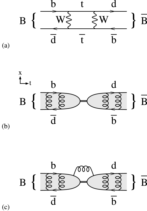
Figure 1.9: (a) One of the two diagrams dominating $B^{0}$-$\bar{B^{0}}$ mixing (the other exchanges $t\leftrightarrow W$). (b) The same diagram emphasizing the Strong force between the quarks and the relative size of the $t$-$W$ loop. (c) Diagrams that contribute to the Bag parameter, which is not a part of $f_{B}$.

Despite this precision, the $V_{td}$ extraction has 20% uncertainties from Strong interactions. To illustrate the influence of the Strong interaction on $B^{0}$-$\bar{B^{0}}$ mixing, we re-draw the Feynman diagram as a space-time diagram in Figure 1.9(b). The $W$-$t$ loop is a very short-range process ($\sim$0.001 fm). By comparison, the average distance between the $b$ and $\bar{d}$ quarks is set by the QCD potential ($\sim$fm), just as it is for $b\bar{b}$ in the $\Upsilon$ meson. Just as in $\Gamma_{ee}$, the rate of $B^{0}$-$\bar{B^{0}}$ mixing is determined by the probability that the two quarks will fluctuate to the same point in space, and this probability is characterized by the $B$ meson decay constant $f_{B}$.

$$\Gamma(B\to\bar{B})=\mbox{(known factors)}\times\bigg{|}\underbrace{{f_{B}}^{2}B_{B}}_{\mbox{\scriptsize QCD}}\times{V_{td}}^{2}\bigg{|}^{2}\mbox{.}$$ (1.3)

The $B^{0}$-$\bar{B^{0}}$ mixing amplitude depends on two factors of $f_{B}$, one from the $B^{0}$ wavefunction and the other from $\bar{B^{0}}$ (see Figure 1.9(b)). Another factor, known as the Bag parameter $B_{B}$, corrects for gluons connecting the $B^{0}$ and $\bar{B^{0}}$ (Figure 1.9(c)). Its uncertainty is more easily controlled. Our knowledge of $V_{td}$ is therefore dominated by the uncertainty in $f_{B}$.

In principle, one can measure $f_{B}$ experimentally through $B^{+}\to\mu^{+}\nu$ or $\tau^{+}\nu$, illustrated in Figure 1.10. The charged $B^{+}$ has different quark content from the neutral $B^{0}$, but its decay rate depends on $f_{B}$ because up and down quark masses are both much smaller than the bottom quark mass, and flavors do not enter the QCD calculation. Unfortunately, this process is suppressed by $V_{ub}$, to the extent that it has yet to be observed in 88.9 million $B^{\pm}$ decays at BaBar [6]. Given the low rate of this decay and the challenge of reconstruction, it will take a long time to accumulate enough data to make a statistically significant measurement of $f_{B}$.

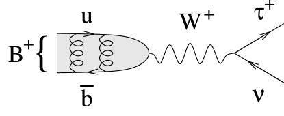
Figure 1.10: Decay diagram of $B^{+}\to\tau^{+}\nu$.

The $B$ decay constant may instead be extracted from Lattice QCD simulations of $B$ mesons in much the same way as $\Gamma_{ee}$ is from $\Upsilon$ simulations: by sampling the wavefunction at the origin. The HPQCD collaboration has found $f_{B}$ to be 216 $\pm$ 22 MeV (see Figure 1.11) [7]. Like the $\Upsilon$, the $B$ meson is modeled with NRQCD, and the discretization issues and corrections to this calculation are analogous to $\Gamma_{ee}$. The largest uncertainty in $f_{B}$ is in the $Z_{\mbox{\scriptsize match}}^{\mbox{\scriptsize axial}}$ constant that matches lattice approximations of the virtual $W^{\pm}$ current to a continuum renormalization scheme. This $Z_{\mbox{\scriptsize match}}^{\mbox{\scriptsize axial vector}}$ has been calculated to first order in $\alpha_{s}$, but uncertainty in the ${\alpha_{s}}^{2}$ term imposes a 9% uncertainty on $f_{B}$, which dominates the 10% uncertainty cited above. Finer calculations of $f_{B}$ are in progress.

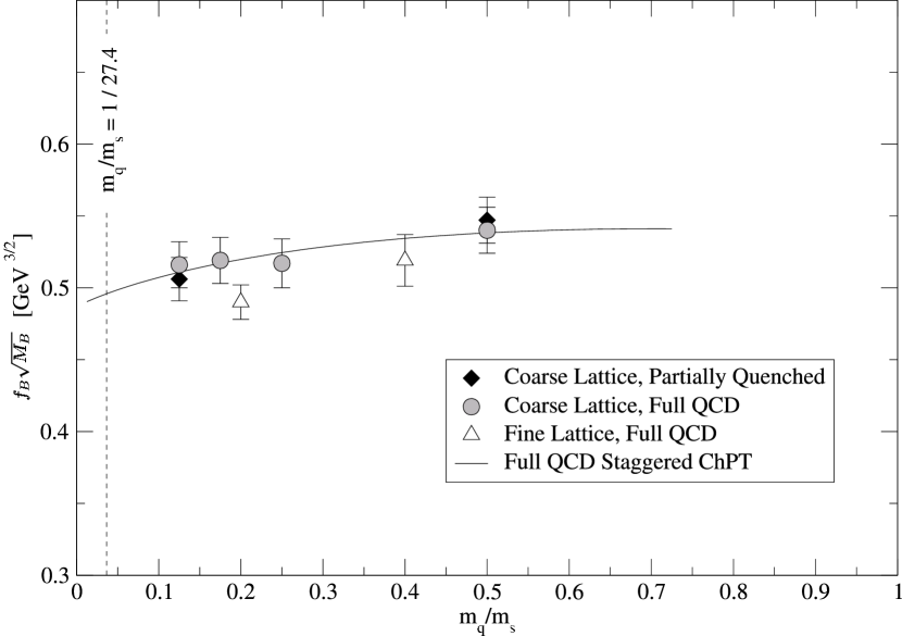
Figure 1.11: HPQCD calculations of $f_{B}\sqrt{M_{B}}$ as a function of the light quark mass used in the simulations. The solid curve extrapolates from the simulations to the natural $m_{q}/m_{s}$ of 1/27.4.

Lattice calculations of $f_{B}$ would be viewed with suspicion if calculations of $\Gamma_{ee}$ do not match experiment at a comparable level of precision. From the lattice’s perspective, the only difference between these two calculations is the mass of one of the two quarks: a bottom quark is replaced by a light quark. This is not a trivial distinction: it is also worthwhile checking the lattice calculation of the $D$ meson decay constant, in which a charm quark and a light quark annihilate, with experimental results from CLEO-c that are now becoming available [8]. The $D$ meson is a heavy/light quark combination, just like the $B$ meson, so $f_{D}$ is physically more analogous to $f_{B}$ than $\Gamma_{ee}$ is. However, the $D$ meson is a more relativistic system, the charm quark being four times lighter than bottom, so instead of simulating charm quarks with NRQCD, the $D$ meson simulations use a relativistic approximation known as the FermiLab action [3]. Thus, $\Gamma_{ee}$ tests the treatment of heavy quarks in the $f_{B}$ calculation and $f_{D}$ tests the heavy-light simulation and matching the virtual $W^{\pm}$ current to the continuum with $Z_{\mbox{\scriptsize match}}^{\mbox{\scriptsize axial}}$. Ratios of $\Gamma_{ee}$ are particularly applicable to this test, since they will be more sensitive to the treatment of heavy quarks than to $Z_{\mbox{\scriptsize match}}^{\mbox{\scriptsize vector}}$ in $\Gamma_{ee}$. Experimental verification of $\Gamma_{ee}$ and $\Gamma_{ee}$ ratio calculations are therefore key to our confidence in $f_{B}$ and the extraction of $V_{td}$.

Chapter 2 Measurement Technique

2.1 Scans of $\Upsilon$ Resonance Production

To determine the decay rate of $\Upsilon\to e^{+}e^{-}$, we use a special strategy available to $e^{+}e^{-}$ colliders: we measure the total cross-section of $e^{+}e^{-}\to\Upsilon$, the time-reversed process. This cross-section is related to the $b\bar{b}$ wavefunction at the origin for the same reason as $\Gamma_{ee}$ (Figure 2.1, an application of crossing symmetry).

$$\int\sigma(e^{+}e^{-}\to\Upsilon)\,dE_{\mbox{\scriptsize CM}}=3{Q_{b}}^{2}\,64\pi^{3}\alpha^{2}\frac{|\psi(0,0,0)|^{2}}{{M_{\Upsilon}}^{4}}$$ (2.1)

where the $dE_{\mbox{\scriptsize CM}}$ integration is performed over $e^{+}e^{-}$ center-of-mass energies [2]. To obtain $\Gamma_{ee}$ in terms of $\int\sigma(e^{+}e^{-}\to\Upsilon)\,dE_{\mbox{\scriptsize CM}}$, we combine the above with Equation 1.1.

$$\Gamma_{ee}=\frac{{M_{\Upsilon}}^{2}}{6\pi^{2}}\int\sigma(e^{+}e^{-}\to\Upsilon)\,dE_{\mbox{\scriptsize CM}}\mbox{.}$$ (2.2)

This is more general than Equations 1.1 and 2.1, which only apply in the non-relativistic limit. In the fully relativistic case, $|\psi(0,0,0)|^{2}$ must be replaced with an integral of wavefunction values near the origin, which cancels in Equation 2.2.

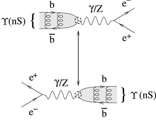
Figure 2.1: Diagrams of $\Upsilon\to e^{+}e^{-}$ and $e^{+}e^{-}\to\Upsilon$. Both feature the same $b$-$\bar{b}$-$\gamma/Z^{0}$ vertex whose rate is set by $|\psi(0,0,0)|^{2}$.

This may seem like a very indirect way of measuring $\Gamma_{ee}$. Why do we not count $\Upsilon\to e^{+}e^{-}$ decays relative to the number of $\Upsilon$ mesons produced, for instance? The reason is because such a fraction would be ${\mathcal{B}}_{ee}$, rather than the decay rate. We would need to multiply by $\Gamma$, the rest mass distribution of the $\Upsilon$ meson, to determine $\Gamma_{ee}$, and this is experimentally inaccessible: $\Gamma$ is on the order of 50 keV, which is about a hundred times narrower than the beam energy spread of an $e^{+}e^{-}$ collider and a thousand times narrower than detector resolution. Equation 2.2 provides direct access to $\Gamma_{ee}$, which, as a collateral benefit, can be combined with ${\mathcal{B}}_{ee}$ to obtain $\Gamma$.

To evaluate $\int\sigma(e^{+}e^{-}\to\Upsilon)\,dE_{\mbox{\scriptsize CM}}$, we fit a curve to the $\Upsilon$ lineshape, that is, the $\Upsilon$ production cross-section as a function of $e^{+}e^{-}$ collision energy. We then integrate this curve analytically. To construct our fit function, we begin with the natural lineshape of the $\Upsilon(1S)$, $\Upsilon(2S)$, and $\Upsilon(3S)$ resonances, a Breit-Wigner:

$$\sigma(e^{+}e^{-}\to\Upsilon)(E_{\mbox{\scriptsize CM}})=\left(\frac{6\pi^{2}}{{M_{\Upsilon}}^{2}}\,\Gamma_{ee}\right)\frac{\Gamma/2\pi^{2}}{(E_{\mbox{\scriptsize CM}}-M_{\Upsilon})^{2}+(\Gamma/2)^{2}}\mbox{.}$$ (2.3)

The observed spectrum is smeared by a unit Gaussian spread in incident beam energies ($\sim$4 MeV), as discussed above. We represent this smearing by a convolution, but the integral is unchanged.

The high-energy side of the lineshape is also distorted by initial-state radiation (ISR): $e^{+}e^{-}\to\Upsilon$ events are hard to distinguish from $e^{+}e^{-}\to\gamma\Upsilon$ for sufficiently small photon energies $E_{\gamma}$. These events add to the apparent cross-section, and contribute a high-energy tail that falls of as $1/E_{\gamma}$, causing the integral to diverge. We could introduce an artificial cut-off, but then the $\Gamma_{ee}$ we report would be a function of that cut-off. Instead, we include the ISR distortion in our fit function to match the data, but report the integral with no ISR contribution, a procedure depicted in Figure 2.2. This means that $\sigma(e^{+}e^{-}\to\Upsilon)$ in Equation 2.2 represents the $\Upsilon$ cross-section with no ISR photons at all, and the $\Gamma_{ee}$ we derive is devoid of final-state radiation ($\Upsilon\to\gamma e^{+}e^{-}$).

Figure 2.2: The anatomy of an $\Upsilon$ lineshape scan (cross-section versus center-of-mass energy), including the natural lineshape (dashed peak), beam energy spread and ISR tail (solid), and backgrounds (vertical offset).

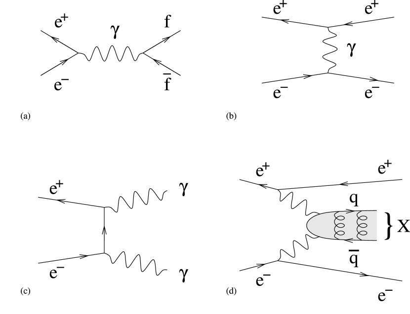
Figure 2.3: Survey of continuum backgrounds: (a) $s$-channel fermion pair production, $f\bar{f}$ may be $q\bar{q}$, $\mu^{+}\mu^{-}$, or $\tau^{+}\tau^{-}$, (b) $t$-channel exchange which dominates Bhabha ($e^{+}e^{-}$) scattering, (c) $e^{+}e^{-}$ annihilation into two real photons (the other, undrawn diagram simply exchanges the identity of the two outgoing photons), (d) fusion of two virtual photons into a low-momentum hadronic state accompanied by high-energy $e^{+}e^{-}$.

In addition to $e^{+}e^{-}\to\Upsilon$ and $\gamma\Upsilon$, electron-positron collisions in the 9.4–10.4 GeV range can also undergo the following continuum processes, which also contribute to the observed cross-section:

1. $q\bar{q}$, $\mu^{+}\mu^{-}$, and $\tau^{+}\tau^{-}$ purely through annihilation ($s$-channel, Figure 2.3(a)),

2. Bhabha $e^{+}e^{-}$ through annihilation ($s$-channel) and Coulomb scattering
   ($t$-channel, Figure 2.3(b)),

3. $\gamma\gamma$ through annihilation (Figure 2.3(c)), and

4. $e^{+}e^{-}X$ via the fusion of two virtual photons from a grazing collision (Figure 2.3(d)).

At these energies, muon- and tau-pair cross-sections are 1 nb, and $q\bar{q}$ are 4 nb, decreasing with center-of-mass energy as $1/s$ ($s={E_{\mbox{\scriptsize CM}}}^{2}$). Bhabha events are by far the most abundant; in fact, the Bhabha cross-section diverges if glancing-angle scatters are included. The $\gamma\gamma$ cross-section diverges also, but less rapidly as a function of angle. Bhabha and $\gamma\gamma$ cross-sections both decrease as $1/s$. The last process, two-photon fusion, generates low-momentum hadronic particles $X$ and two electrons ($e^{+}e^{-}$), at least one of which grazes the incident beam-line. The two-photon fusion cross-section increases with center-of-mass energy, but very slowly, as $\log s$. Some of these non-$\Upsilon$ processes can be hard to distinguish or are indistinguishable from $\Upsilon$ events, and therefore can be confused with signal. Fortunately, the continuum cross-section is a much smoother function of $E_{\mbox{\scriptsize CM}}$ than the $\Upsilon$ cross-section, so the $\Upsilon$ peak appears to stand on a flat continuum plateau, also depicted in Figure 2.2. We add terms to the fit function to accommodate these effects as well.

When a continuum final state is truly indistinguishable from an $\Upsilon$ decay, as is the case for $e^{+}e^{-}\to q\bar{q}$ and $e^{+}e^{-}\to\Upsilon\to q\bar{q}$, the cross-sections don’t simply add. The complex amplitudes for these processes add, the square of which is proportional to cross-section:

$$\sigma_{{\mbox{\scriptsize res}}+{\mbox{\scriptsize cont}}}(E_{\mbox{\scriptsize CM}})\propto\big{|}{\mathcal{A}}_{\mbox{\scriptsize res}}+{\mathcal{A}}_{\mbox{\scriptsize cont}}\big{|}^{2}=\big{|}{\mathcal{A}}_{\mbox{\scriptsize res}}\big{|}^{2}+\big{|}{\mathcal{A}}_{\mbox{\scriptsize cont}}\big{|}^{2}+2{\mathcal{R}e}({{\mathcal{A}}_{\mbox{\scriptsize res}}}^{*}{\mathcal{A}}_{\mbox{\scriptsize cont}})\mbox{,}$$ (2.4)

so we can re-write $\sigma_{{\mbox{\scriptsize res}}+{\mbox{\scriptsize cont}}}$ as

$$\sigma_{{\mbox{\scriptsize res}}+{\mbox{\scriptsize cont}}}(E_{\mbox{\scriptsize CM}})=\sigma_{\mbox{\scriptsize res}}(E_{\mbox{\scriptsize CM}})+\sigma_{\mbox{\scriptsize cont}}(E_{\mbox{\scriptsize CM}})+\tilde{\sigma}_{\mbox{\scriptsize int}}(E_{\mbox{\scriptsize CM}})$$ (2.5)

where $\sigma$ denotes cross-section and ${\mathcal{A}}$ amplitude, “res” for the resonant ($\Upsilon$) contribution and “cont” for the continuum. The interference term, $\tilde{\sigma}_{\mbox{\scriptsize int}}$, is a function of $E_{\mbox{\scriptsize CM}}$, like the familiar $\sigma_{\mbox{\scriptsize res}}$ and $\sigma_{\mbox{\scriptsize cont}}$, but it can be negative and sometimes larger than $\sigma_{\mbox{\scriptsize res}}$. That is, introducing another way for $e^{+}e^{-}$ to produce $q\bar{q}$ can actually decrease the $q\bar{q}$ cross-section! We calculate this interference term from a Breit-Wigner amplitude (Feynman propagator) of the form

$${\mathcal{A}}_{\mbox{\scriptsize res}}\propto\frac{1}{E_{\mbox{\scriptsize CM}}-M_{\Upsilon}+i\Gamma/2}$$ (2.6)

and a constant continuum with constant phase $\phi_{0}$ (resonance phase minus continuum phase at $E_{\mbox{\scriptsize CM}}\ll M_{\Upsilon}$). We find

$$\tilde{\sigma}_{\mbox{\scriptsize int}}(E_{\mbox{\scriptsize CM}}) = \alpha_{\mbox{\scriptsize int}}\,\sigma_{\mbox{\scriptsize res}}(E_{\mbox{\scriptsize CM}})\,\left(2\frac{E_{\mbox{\scriptsize CM}}-M_{\Upsilon}}{\Gamma}\cos\phi_{0}+\sin\phi_{0}\right)$$ (2.7)

$$\mbox{where }\alpha_{\mbox{\scriptsize int}} = \sqrt{\sigma_{\mbox{\scriptsize cont}}\,({M_{\Upsilon}}^{2}/3\Gamma_{ee})\,\Gamma_{f}}\mbox{.}$$ (2.8)

The magnitude of each interference correction is characterized by $\alpha_{\mbox{\scriptsize int}}$, which is a constant derived from the continuum cross-section, the resonance magnitude $\Gamma_{ee}$, and the decay rate $\Gamma_{f}$ to the given final state (in this case $q\bar{q}$). Given the continuum $q\bar{q}$ cross-section (through $R=\sigma(e^{+}e^{-}\to q\bar{q})/\sigma(e^{+}e^{-}\to\mu^{+}\mu^{-})$ [9]) and the resonance $q\bar{q}$ branching ratio $\Gamma_{q\bar{q}}/\Gamma_{ee}$ (assuming ${\mathcal{B}}_{ee}$ = ${\mathcal{B}}_{\mu\mu}$, this is $R$), we calculate $\alpha_{\mbox{\scriptsize int}}$ to be 0.0186, 0.0179, and 0.0182 for the $\Upsilon(1S)$, $\Upsilon(2S)$, and $\Upsilon(3S)$, respectively, with 3% uncertainties. Note that if $\phi_{0}=0$, $\tilde{\sigma}_{\mbox{\scriptsize int}}<0$ below $M_{\Upsilon}$ and $\tilde{\sigma}_{\mbox{\scriptsize int}}>0$ above $M_{\Upsilon}$. If, however, $\phi_{0}=\pm\pi/2$, $\tilde{\sigma}_{\mbox{\scriptsize int}}$ will have exactly the same energy dependence as $\sigma_{\mbox{\scriptsize res}}$, and thus be indistinguishable from the $\Upsilon$ cross-section itself.

Continuum Bhabhas, $\mu^{+}\mu^{-}$, $\tau^{+}\tau^{-}$, and $q\bar{q}$ all interfere with $e^{+}e^{-}\to\Upsilon\to f\bar{f}$ with phase angle $\phi_{0}=0$. We can see this by considering that all of these processes are purely QED except for the formation, propagation, and disintegration of the $\Upsilon$ resonance. The tree-level QED amplitudes are real because they all feature an even number of photon vertices (each of which contributes a factor of $i$). While $\Upsilon$ production introduces a factor of the conjugated wavefunction at the origin, $\psi(0,0,0)^{*}$, the $\Upsilon$ decay part of the diagram multiplies it by $\psi(0,0,0)$. The $\Upsilon$ propagator (Equation 2.6) is real for $E_{\mbox{\scriptsize CM}}$ $\ll$ $M_{\Upsilon}$. Therefore, $\phi_{0}=0$ or $\phi_{0}=\pi$. We see in a scan of $\Upsilon(1S)\to\mu^{+}\mu^{-}$ (Figure 2.4) that interference is destructive below resonance and constructive above, which indicates $\phi_{0}=0$.

Figure 2.4: Efficiency-corrected, background-subtracted $\mu^{+}\mu^{-}$ cross-section versus $E_{\mbox{\scriptsize CM}}$, fitted with (a) resonance, continuum, and interference normalization allowed to float independently, and (b) interference fixed with the opposite phase. The fit prefers $\phi_{0}=0$ over $\phi_{0}=\pi$ by 18.5 standard deviations.

2.2 $\Upsilon$ Final States and Hadronic Cross-section

In our $e^{+}e^{-}$ collisions, $\Upsilon$ mesons are produced nearly at rest and immediately decay. We only ever observe the $\Upsilon$ decay products. An $\Upsilon$ may decay into

1. leptonic final states: $e^{+}e^{-}$, $\mu^{+}\mu^{-}$, and $\tau^{+}\tau^{-}$, through an $s$-channel virtual photon (or $Z^{0}$, with 1.5% contribution to the rate),

2. hadronic final states via the hadronization of $q\bar{q}$, $ggg$, or $gg\gamma$,

3. lower-mass $b\bar{b}$ states, accompanied by pions or photons,

4. neutrino pairs exclusively through $Z^{0}$, and

5. possibly other, exotic, modes.

The $\mu^{+}\mu^{-}$ branching fractions, ${\mathcal{B}}_{\mu\mu}$, have been measured with 2–5% precision for the $\Upsilon(1S)$, $\Upsilon(2S)$, and $\Upsilon(3S)$ [12], and the $e^{+}e^{-}$ and $\tau^{+}\tau^{-}$ decays are expected to have the same amplitudes as $\mu^{+}\mu^{-}$. Thus, the branching fractions, ${\mathcal{B}}_{ee}$, ${\mathcal{B}}_{\mu\mu}$, and ${\mathcal{B}}_{\tau\tau}$, are nearly equal, with only a tiny correction from lepton mass, which is 0.05% for the heavy $\tau$ lepton. This assumption is called Lepton Universality.

States containing bare quarks or gluons (partons), like $q\bar{q}$, $ggg$, and $gg\gamma$, must hadronize before propagating to the detector. That is, strings of self-interacting gluons, stretched between the partons, will generate new quark/anti-quark pairs when stretched sufficiently far. These new quarks will clothe the original partons, such that a macroscopic detector will only ever observe mesons ($q\bar{q}$ bound states) and baryons ($qqq$ or $\bar{q}\bar{q}\bar{q}$). Hadronization is a random process, leading to a broad spectrum of event topologies, with as many as twenty particles in the final state. Most $\Upsilon$ mesons decay hadronically.

Only the $\Upsilon(2S)$ and the $\Upsilon(3S)$ have appreciable decay rates to other $b\bar{b}$ states. (The $\Upsilon(1S)\to\eta_{b}(1S)$ branching fraction is expected to be less than $10^{-4}$ [13].) These decays are the bottomonium equivalent of atomic transitions, but in addition to emitting monoenergetic photons in $\Delta J=1$ decays, bottomonium can emit monoenergetic $\pi\pi$ (charged or neutral) and $\gamma\gamma$ when decaying with $\Delta J=0$. Figure 2.5 plots the energy levels of the most well-known $b\bar{b}$ states and the transitions between them.

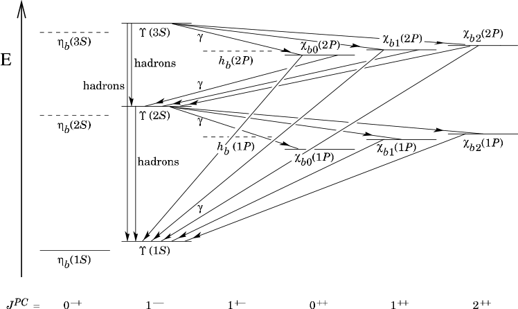
Figure 2.5: States and transitions in the $b\bar{b}$ system. Only $J=1$ $\Upsilon$ mesons are produced directly by $e^{+}e^{-}$, and of those, only $\Upsilon(2S)$ and $\Upsilon(3S)$ decay significantly into lower $b\bar{b}$ states.

The $Z^{0}$ boson at $\Upsilon$ masses is 80 GeV off-shell, while the photon is only 10 GeV off shell, so the $Z^{0}$ contributes to 1.5% of the $\Upsilon$ meson’s Electroweak decays ($e^{+}e^{-}$, $\mu^{+}\mu^{-}$, $\tau^{+}\tau^{-}$, and $q\bar{q}$). The Electroweak decays account for $(3+R){\mathcal{B}}_{\mu\mu}$ = 16% of all $\Upsilon$ decays, where $R$, the branching ratio of $q\bar{q}$ to $\mu^{+}\mu^{-}$, has a value of 3.58 $\pm$ 0.14 [9]. The $\Upsilon\to Z^{0}$ branching fraction is therefore 0.25%, and $\Upsilon\to Z^{0}\to\nu\bar{\nu}$ is 0.05%, which is negligible at our level of precision.

Finally, we do not exclude the possibility that unknown $\Upsilon$ decays exist, or that their branching fractions are larger than a few percent. These modes may resemble hadronic decays, or have exotic signatures that have been overlooked.

For the sake of this analysis, we will classify $\Upsilon$ decay modes as “leptonic,” meaning $e^{+}e^{-}$, $\mu^{+}\mu^{-}$, and $\tau^{+}\tau^{-}$ exclusively (no $\nu\bar{\nu}$), or “hadronic,” meaning everything else. By this designation, there are “hadronic” final states that contain no hadrons at all, such as the $\Upsilon(2S)\to\gamma\chi_{b1}(1P)\to\gamma\gamma\Upsilon(1S)\to\gamma\gamma e^{+}e^{-}$ chain, $\Upsilon\to\nu\bar{\nu}$, and $\Upsilon\to\mbox{\sc wimp }\overline{\mbox{\sc wimp}}$ (where wimps are cosmologically-motivated invisible particles). This classification is convenient and has been used by previous $\Gamma_{ee}$ analyses.

Experimentally, the $\Upsilon$ cross-section is the number of $e^{+}e^{-}\to\Upsilon$ events that occurred divided by the time-integrated luminosity of the $e^{+}e^{-}$ collisions. To identify $e^{+}e^{-}\to\Upsilon$ events, we select events that look like hadronic $\Upsilon$ decays, because the leptonic final states are hard to distinguish from continuum backgrounds and account for only 6–7.5% of the $\Upsilon$ decays. Thus, we count $e^{+}e^{-}\to\Upsilon\to\mbox{hadronic}$ events and our cross-section is $\sigma(e^{+}e^{-}\to\Upsilon\to\mbox{hadronic})$. This hadronic cross-section is a constant multiple of the total cross-section

$$\sigma(e^{+}e^{-}\to\Upsilon\to\mbox{hadronic})=\sigma(e^{+}e^{-}\to\Upsilon)\times\Gamma_{\mbox{\scriptsize had}}/\Gamma_{\mbox{\scriptsize tot}}$$ (2.9)

for all $E_{\mbox{\scriptsize CM}}$. We fit our lineshape function to hadronic cross-section versus $E_{\mbox{\scriptsize CM}}$ data and thereby derive $\Gamma_{ee}\Gamma_{\mbox{\scriptsize had}}/\Gamma_{\mbox{\scriptsize tot}}$. To obtain $\Gamma_{ee}$, we divide by ${\mathcal{B}}_{\mbox{\scriptsize had}}=\Gamma_{\mbox{\scriptsize had}}/\Gamma_{\mbox{\scriptsize tot}}$, which is $(1-{\mathcal{B}}_{ee}-{\mathcal{B}}_{\mu\mu}-{\mathcal{B}}_{\tau\tau})$ by definition. Applying Lepton Universality, we use

$$\Gamma_{ee}=\frac{\Gamma_{ee}\Gamma_{\mbox{\scriptsize had}}/\Gamma_{\mbox{\scriptsize tot}}}{1-3{\mathcal{B}}_{\mu\mu}}$$ (2.10)

to take advantage of the well-measured ${\mathcal{B}}_{\mu\mu}$. With $\Gamma_{ee}$, we again assume ${\mathcal{B}}_{ee}={\mathcal{B}}_{\mu\mu}$ to calculate $\Gamma=\Gamma_{ee}/{\mathcal{B}}_{\mu\mu}$.

The upcoming chapters will each present one aspect of the $\Gamma_{ee}\Gamma_{\mbox{\scriptsize had}}/\Gamma_{\mbox{\scriptsize tot}}$ measurement.

Chapter 3

will describe the $e^{+}e^{-}$ collider and particle detector that were used to generate and count $e^{+}e^{-}\to\Upsilon\to\mbox{hadronic}$ events.

Chapter 4

will define the $e^{+}e^{-}\to\Upsilon\to\mbox{hadronic}$ selection criteria and explain how background events are removed from that count.

Chapter 5

will derive the correction for hadronic $\Upsilon$ events missing from the sample, that is, the efficiency of the selection criteria.

Chapter 6

will explain how we measure integrated luminosity, thereby converting our hadronic event counts into hadronic cross-sections.

Chapter 7

will show how we use cross-section data to put an upper limit on the uncertainty in beam energy measurements.

Chapter 8

will describe the fit function and fit results in detail, and

Chapter 9

will present all $\Gamma_{ee}\Gamma_{\mbox{\scriptsize had}}/\Gamma_{\mbox{\scriptsize tot}}$, $\Gamma_{ee}$, $\Gamma$, and $|\psi(0,0,0)|^{2}$ results.

Chapter 3 Collider and Detector

In this Chapter, we present the apparatus we used to collide electrons and positrons and collect $\Upsilon$ decay products.

3.1 Cornell Electron Storage Ring

Our electron-positron pairs collided in the Cornell Electron Storage Ring (CESR), a 768 m-circumference, symmetric storage ring and collider in Ithaca, NY. This collider covers a very broad range of $e^{+}e^{-}$ energies, from the charmonium region at $E_{\mbox{\scriptsize beam}}=E_{\mbox{\scriptsize CM}}/2=$ 1.8 GeV through the excited $\Upsilon$ states at 5.5 GeV. The $\Upsilon(1S)$, $\Upsilon(2S)$, and $\Upsilon(3S)$ masses, between 4.7 and 5.2 GeV, lie in CESR’s optimal range. In fact, scans of the $\Upsilon(1S)$ through $\Upsilon(3S)$ are among the first data taken by CESR in 1979 (Figure 3.1).

Figure 3.1: Greeting card from CESR in 1979, demonstrating its success in colliding $e^{+}e^{-}$ at 10 GeV by scanning the lineshapes of the $\Upsilon(1S)$, $\Upsilon(2S)$, and $\Upsilon(3S)$ (left to right).

Copper dipole magnets confine the beams to their orbits, alternating with quadrapole and sextapole magnets for focusing. Superconducting quadruples provide the final focusing of the beams, only 30 cm from the interaction point, allowing the collisions to reach instantaneous luminosities of $10^{33}$ cm^-2 s^-1. Like all synchrotrons, the beam is pulsed to permit acceleration: beam bunches are timed to enter radio frequency (RF) standing waves just when the electric field is maximal. In CESR, nine trains of five bunches circulate in the ring at once, with 1.15$\times 10^{10}$ particles per bunch. Both the electron beam and the positron beam are enclosed in the same beam-pipe, so they need to be separated electrostatically. The resulting orbit is called a “pretzel orbit” because the beams twine around each other like twisted pair cable.

We determine the beam energy by measuring the magnetic field in two dipole magnets, outside the ring but otherwise identical to the others. The current supplied to these two test magnets is in series with the beam magnets to assure the same current, and the magnetic field is measured with nuclear magnetic resonance (NMR) probes. The naïve beam energy,

$$E_{\mbox{\scriptsize beam}}=\mbox{electron charge}\times\mbox{magnetic field}\times\mbox{CESR radius}$$ (3.1)

is then corrected for shifts in the RF frequency, steering and focusing magnet currents, and the voltage of the electrostatic separators. This full reckoning misses the true beam energy by 0.172%, which is 18 MeV in $E_{\mbox{\scriptsize CM}}$ near the $\Upsilon$ masses, but it is very stable with time and tracks beam energy differences with the same precision. Such a beam energy measurement will not improve the world knowledge of $\Upsilon$ masses, but the scale uncertainty is small enough to have negligible impact on the width, and therefore the area, of the resonance scans.

Distributions of electron and positron energies in the CESR beam are 0.057% wide at the $\Upsilon(1S)$ (this is the ratio of the standard deviation to the mean) and this width scales linearly with beam energy. The beam energy distribution is Gaussian. Our lineshape data, which is the world’s most sensitive test of $e^{+}e^{-}$ beam energy distributions near 10 GeV, show no deviations from a pure Gaussian distribution.

The beam energy spread can vary by as much as 1–2% a month, due to perturbations in the beams’ orbits from environmental conditions. We observed such a shift (Figure 3.2), coincident with large corrections to the horizontal steering magnets to compensate for the new orbit. We use records of these changes to track potential shifts in the beam energy spread, and allow shifts in the widths of the lineshapes by adding floating parameters to the fit.

Figure 3.2: Beam energy spread fit results in the center-of-mass ($\Delta E=\sqrt{2}$ single beam energy spread) divided by $E_{\mbox{\scriptsize CM}}$², which is nearly constant, as expected. The third $\Upsilon(1S)$ measurement (April 2002) is 2.4% lower than the second (March 2002).

The beam-beam interaction region is a ribbon 0.18 mm tall (out of the ring plane), 0.34 mm wide (in the ring plane but perpendicular to the beam axis), and 1.8 cm long (in the ring, along the beam axis). Electrons and positrons may collide anywhere within this constrained distribution, and its center drifts by about 4 mm along the beam-line and 1–2 mm perpendicular to it on a monthly timescale. We can easily track these changes.

In addition to $e^{+}e^{-}$ collisions, beam particles can interact with gas nuclei inside the beam-pipe and with the wall of the beam-pipe itself (2.1 cm in radius). To minimize the number of beam-gas events, the beam-pipe is kept evacuated at 2–4$\times 10^{-8}$ torr. Beam-wall events are minimized by focusing. The electron and positron currents can vary independently, so electron-induced beam-gas and beam-wall and positron-induced beam-gas and beam-wall rates are not identical. In fact, we find that positron-induced rates are typically twice electron-induced rates, suggesting a difference in cross-sections.

We collected data in eleven dedicated scans of the $\Upsilon(1S)$ and one high-energy point (100 MeV above the $\Upsilon(1S)$ mass), totalling 0.09 fb^-1, and added to this 18 fb^-1 of subsequent on-resonance peak data (adjacent in time and limited to 48 hours after the beginning of the scan). We obtained six $\Upsilon(2S)$ scans with a high-energy point (60 MeV above the $\Upsilon(2S)$ mass), totalling 0.05 fb^-1  and added 0.03 fb^-1 of subsequent peak data, and seven $\Upsilon(3S)$ scans with a high-energy point (45 MeV above the $\Upsilon(3S)$ mass), totalling 0.08 fb^-1, and added 14 fb^-1 of subsequent peak data. We present all the individual scans in Table 3.1. In addition to scan data, we used the full 0.19 fb^-1, 0.41 fb^-1, and 0.14 fb^-1 off-resonance datasets, 20 MeV below the $\Upsilon(1S)$, $\Upsilon(2S)$, and $\Upsilon(3S)$ masses, to subtract continuum backgrounds.

Table 3.1: Scans of the $\Upsilon(1S)$, including associated on-resonance peak data. “Spread” indicates groups of scans which have the same beam energy spread (same labels as in Figure 3.2). The last entry is a point taken 100 MeV above the $\Upsilon(1S)$ mass.

Scan	Int. Lum. (pb-1)	Run Range	Dates	Spread
jan16	6.7	123164–123178	Jan. 15–16, 2002	$\Upsilon(1S)_{1}$
jan30	52.7	123596–123645	Jan. 30–Feb.  1, 2002	$\Upsilon(1S)_{1}$
feb06	26.3	123781–123836	Feb.  6–8, 2002	$\Upsilon(1S)_{1}$
feb13	7.8	124080–124092	Feb. 19–20, 2002	$\Upsilon(1S)_{1}$
feb20	21.0	124102–124159	Feb. 20–22, 2002	$\Upsilon(1S)_{1}$
feb27	23.9	124279–124338	Feb. 27–Mar.  1, 2002	$\Upsilon(1S)_{2}$
mar06	19.6	124436–124495	Mar.  6–8, 2002	$\Upsilon(1S)_{2}$
mar13	25.9	124625–124681	Mar. 13–15, 2002	$\Upsilon(1S)_{2}$
apr08	7.2	125254–125262	Apr.  8–9, 2002	$\Upsilon(1S)_{3}$
apr09	5.6	125285–125295	Apr.  9–10, 2002	$\Upsilon(1S)_{3}$
apr10	42.3	125303–125358	Apr. 10–12, 2002	$\Upsilon(1S)_{3}$
+100 MeV	11.6	124960–124973	Mar. 27–28, 2002

Table 3.2: Scans of the $\Upsilon(2S)$ and $\Upsilon(3S)$, including associated on-resonance peak data. “Spread” indicates groups of scans which have the same beam energy spread (same labels as in Figure 3.2). The “+60 MeV” and “+45 MeV” entries are points taken 60 and 45 MeV above the $\Upsilon(1S)$ and $\Upsilon(3S)$ masses, respectively. The dates of the “+45 MeV” data-taking overlap the “dec26” scan, but the integrated luminosity we quote do not.

Scan	Int. Lum. (pb-1)	Run Range	Dates	Spread
may29	14.6	126449–126508	May. 29–31, 2002	$\Upsilon(2S)$
jun11	9.9	126776–126783	Jun. 11–12, 2002	$\Upsilon(2S)$
jun12	23.6	126814–126871	Jun. 12–14, 2002	$\Upsilon(2S)$
jul10	18.8	127588–127615	Jul. 10–11, 2002	$\Upsilon(2S)$
jul24	5.8	127924–127933	Jul. 23–24, 2002	$\Upsilon(2S)$
aug07	9.3	128303–128316	Aug.  7–8, 2002	$\Upsilon(2S)$
+60 MeV	4.9	127206–127219	Jun. 26–27, 2002
nov28	27.5	121884–121940	Nov. 28–30, 2001	$\Upsilon(3S)_{1}$
dec05	41.3	122069–122126	Dec.  6–8, 2001	$\Upsilon(3S)_{2}$
dec12	41.3	122245–122298	Dec. 12–14, 2001	$\Upsilon(3S)_{3}$
dec19	24.2	122409–122452	Dec. 19–22, 2001	$\Upsilon(3S)_{4}$
dec26	27.7	122535–122579	Dec. 25–26, 2001	$\Upsilon(3S)_{5}$
jan02	27.7	122766–122821	Jan.  2–4, 2002	$\Upsilon(3S)_{6}$
jan09	44.5	122993–123044	Jan.  9–11, 2002	$\Upsilon(3S)_{7}$
+45 MeV	10.8	122568–122575	Dec. 26, 2001

3.2 CLEO Detector

The CLEO detector is a general-purpose assembly of detectors built concentrically around the CESR interaction point [10] [11]. This analysis uses only three of CLEO’s detectors: the silicon vertex detector and central drift chamber for identifying charged particles, and the CsI crystal calorimeter for measuring electron and photon energies, and for simple particle identification. The CLEO-III apparatus, which is the generation of CLEO in operation in 2001–2002, is depicted in Figure 3.3.

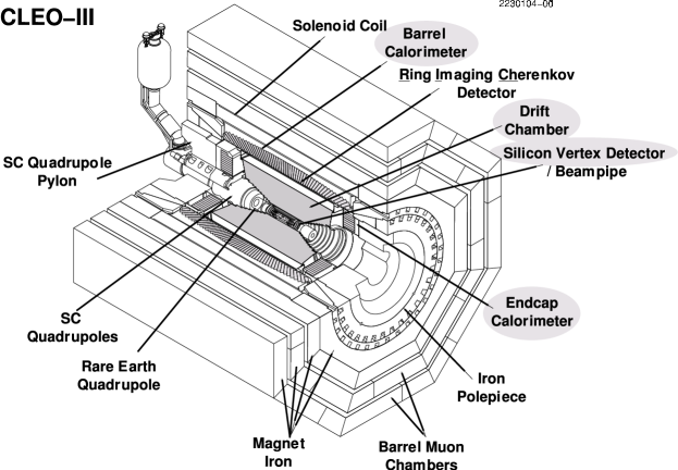
Figure 3.3: An isometric view of the CLEO-III detector, highlighting the silicon vertex detector, the drift chamber, and the CsI crystal calorimeter in gray.

We define the $z$ axis of our coordinate system to be parallel with the beam-line, pointing in the direction of the incident positron current (west). Our coordinate system is right-handed, with $y$ pointing up and $x$ pointing away from the center of the CESR ring (south). The origin of the coordinate system is at the center of the drift chamber, and lies within 1–2 mm of the beam-beam collision point. This coordinate system is illustrated in Figure 3.4. The CLEO detector has an approximate cylindrical symmetry around $z$, so we also define the polar angle $\theta$ of a particle trajectory originating at the origin to be the angle between the trajectory and the beam-line, or $\theta=\tan^{-1}\left(\sqrt{x^{2}+y^{2}}/z\right)$. We often use $\cos\theta$ and $\cot\theta$ to describe the polar angle. The azimuthal angle $\phi$ is the angle for which $\cos\phi=x/\sqrt{x^{2}+y^{2}}$ and $\sin\phi=y/\sqrt{x^{2}+y^{2}}$.

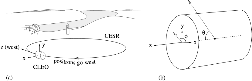
Figure 3.4: Coordinate system of the CLEO detector: (a) orientation with respect to the CESR ring and the Earth, (b) definition of $\theta$ and $\phi$.

The silicon vertex detector and the drift chamber both detect tracks left by charged particles by collecting charge left in the wake of ionizing, high-energy particles. In the vertex detector, the ionized medium is silicon, cut into strips held perpendicular to the trajectories of most particles (Figure 3.5). The charge is conducted out of the detector for amplification along traces which are parallel to the beam-line on one side of the strip and perpendicular to it on the other, so that the two-dimensional point of intersection may be reconstructed.

Figure 3.5: Silicon vertex detector geometry, projected onto the $x$-$y$ plane. The trajectories of central ($\theta\approx\pi/2$) collision products (dashed lines) are roughly perpendicular to the wafers of silicon. Triangles represent diamond rods holding the wafers in place.

In the drift chamber, high-energy charged particles ionize a helium-propane gas (60% He, 40% C₃H₈) in a strong electric field generated by wires strung across the detector volume, parallel with the $z$ axis. One quarter of these wires, called sense wires, are held at $+$2100 V, and the remaining three quarters, called field wires, are held at ground. The resulting field causes the freed electrons to drift away from the field wires toward the sense wire, which conducts the charge to amplifiers for analysis (Figure 3.6). As the electrons drift several millimeters toward the sense wire, they ionize more atoms, causing an avalanche that provides a 10⁷ amplification. We measure the time between the first ionization (estimated from bunch collision times) and charge collection on the sense wire to reconstruct the distance of closest approach of the high-energy charged particle to the sense wire, through the known electron drift speed of 28 $\mu$m/ns. This technique provides an average resolution of 88 $\mu$m in the $x$-$y$ plane. Sensitivity to $z$ position is obtained by tilting the outer wires, presented in more detail in Figure 3.7. The outer 31 layers of wires, called the stereo section, are tilteded 21–28 mrad, yielding a $z$ position resolution of 3–4 mm at each wire. The inner 16 layers, called the axial section, are untilted.

                 

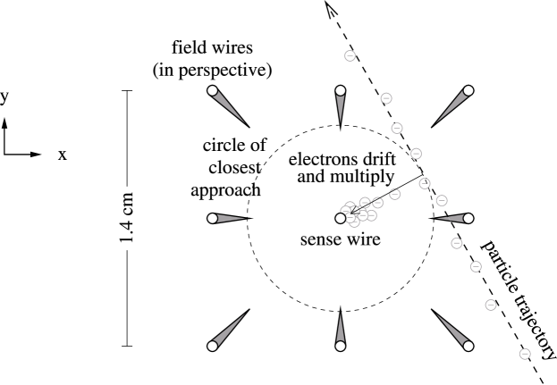
Figure 3.6: Charge collection and multiplication in the drift chamber.

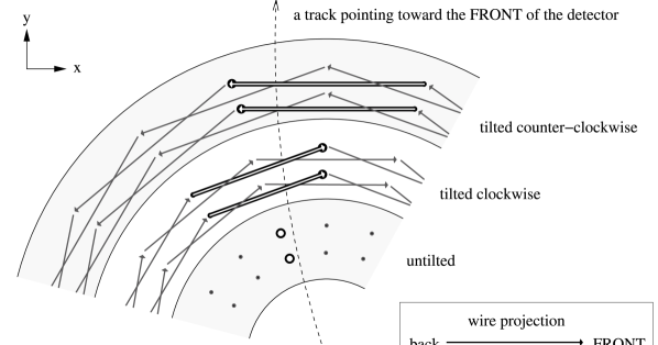
Figure 3.7: Using tilted wires to obtain $z$ information in the drift chamber. Tilted wires extrude lines in the $x$-$y$ projection; position along a tilted wire indicates the $z$ of the track helix near that wire. The closest wires to the track (in three dimensions) are highlighted.

Both tracking volumes are permeated by a 1.5 T magnetic field, pointing along the $z$ axis. Charged particle trajectories are helical in this field: projections onto the $x$-$y$ plane are circles. The polar angle $\theta$ of such a helical trajectory is a constant of the motion, but not $\phi$. We measure the charge $\times$ momentum of particles through the radii of curvature of their tracks. Only electrons, muons, pions, kaons, protons, and deuterons are sufficiently stable and abundantly produced to be observed as tracks, and all of these particles have $\pm$1 units of charge, so the radius of curvature provides access to momentum. The momentum resolution, dominated by drift chamber measurements, is 0.9% for beam-energy tracks, and position resolution near the interaction point, dominated by silicon vertex measurements, is 40 $\mu$m in $x$-$y$ and 90 $\mu$m in $z$.

The outer radius of the drift chamber is 80 cm from the interaction point, and the outer edges are $\pm$110 cm in $z$. The drift chamber’s $z$ range is more limited for smaller radii to accommodate the focusing quadrapole magnet, as shown in Figure 3.8. It will later be to useful to know that charged particles with more than 60 MeV of $z$-momentum exit the detector before completing one half-orbit in the magnetic field. Such particles cannot generate multiple tracks by spiralling inside the detector volume.

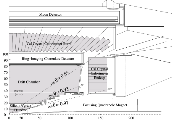
Figure 3.8: A quarter of the CLEO detector, highlighting the silicon vertex detector, the drift chamber, and the CsI crystal calorimeter in gray. Radial and $z$ distances are in centimeters; the angular reach of the calorimeter barrel, the drift chamber, and the calorimeter endcap are illustrated by dashed lines.

The CsI crystal calorimeter is sensitive to photons as well as charged particles, by presenting a transparent, high-$Z$ material for them to interact with Electromagnetically. (Our thallium-doped CsI has a radiation length of 1.83 cm.) Incident electrons and photons are destroyed by this interaction, and replaced by a shower of equal total energy in less energetic photons, electrons, and positrons. Other particles deposit only a fraction of their energy. Visible light from the shower is collected on the back of the 30 cm-long crystals, from which the incident energy is reconstructed. Electrons and photons with energies near the 5 GeV beam energy are fully reconstructed with 1.5% resolution, but the energies of other particles is underestimated. Muons, for instance, deposit only 200 MeV in the calorimeter, regardless of incident energy. Combining the energy of calorimeter showers with track momenta is sufficient to identify and distinguish $e^{+}e^{-}$, $\mu^{+}\mu^{-}$, and $\gamma\gamma$ events with negligible backgrounds.

The calorimeter geometry is composed of three parts: a barrel surrounding the tracking volume and two endcaps, beyond the tracking volume in $z$ (see Figure 3.8). The calorimeter barrel covers polar angles with $|\cos\theta|<0.85$ and the endcaps extend this range to $|\cos\theta|<0.97$. The angular limits of the tracking volume is between these two: $|\cos\theta|<0.93$.

When a threshold amount of activity is observed in the drift chamber and calorimeter, readout electronics are triggered to acquire a snapshot of the detector and record all signals as an event. This activity is quantified in terms of the number of observed tracks and the number of showers above given energy thresholds. For speed in triggering, tracks are counted using a lookup table of drift chamber hits, trained by a simulation, and showers are approximated by summing calorimeter barrel output over 2$\times$2 tiles, called clusters, and counting the number that surpass a given threshold. The number of AXIAL tracks is the number of tracks reconstructed in the axial section of the drift chamber, and STEREO is the number of tracks which can be extended into the stereo section. A CBLO cluster exceeds 150 MeV, a CBMD exceeds 750 MeV, and a CBHI exceeds 1500 MeV. Real showers can be distributed over as many as four tiles, sometimes dividing their energy such that none of the clusters reach a threshold. This is a source of trigger inefficiency for final states that rely on shower information (Figure 3.9). After the data have been recorded, we reconstruct tracks and showers with much finer precision.

Figure 3.9: The efficiencies of CBLO, CBMD, and CBHI identification as a function of fully-reconstructed shower energies for isolated showers. The efficiency curves are not symmetric around their thresholds because shower energy may be divided among tiles.

We use several triggers to accept events, all of which are minimum-thresholds: an event is never rejected for having too many tracks or clusters. All of these triggers are active, and when an event is recorded, it is tagged with the names of the triggers it satisfied. The trigger relevant for this analysis are

• two-track, which requires $\geq$2 AXIAL tracks, prescaled by a factor of 19 (5.3% of the events satisfying this criterion are accepted),

• hadron, which requires $\geq$3 AXIAL tracks and $\geq$1 CBLO,

• rad-tau, which requires $\geq$2 STEREO tracks and ($\geq$1 CBMD or $\geq$2 CBLO),

• $e^{\pm}$-track, which requires $\geq$1 AXIAL track and $\geq$1 CBLO, and

• barrel-bhabha, which requires 2 CBHI clusters on opposite sides of the calorimeter barrel.

To count hadronic $\Upsilon$ decays, we select only those events which satisfied hadron, rad-tau, or $e^{\pm}$-track, the three triggers that are efficient for hadronic decays. (This simplifies our efficiency study.) Note that a minimal condition for these three trigger is that at least one AXIAL track and one CBLO were observed. This minimal requirement is exact because STEREO tracks, being extensions of AXIAL tracks, are always less numerous than or equal in number to AXIAL tracks, and CBMD clusters are also CBLO clusters.

Electron and positron beams are circulated in CESR for about an hour before their currents are exhausted from collisions. Data collected during this time is called a run, and is given a unique, ascending 6-digit identifier. Runs are the basic unit of CLEO data samples; in lineshape scans, we generally took one run at each $E_{\mbox{\scriptsize CM}}$ point at a time.

For some studies, we must simulate our entire detector on a computer. Such Monte Carlo simulations are most important in determining the efficiency-corrected cross-section for Bhabhas in CLEO, which is needed to measure the integrated luminosity of our datasets. While the total Bhabha cross-section is infinite, the efficiency-corrected cross-section, defined by observed Bhabhas, is finite and must be calculated theoretically. This calculation has two ingredients, the differential cross-section as a function of $\theta$ and CLEO’s efficiency for Bhabhas as a function of $\theta$. The first ingredient is calculated with perturbative Quantum Electrodynamics (QED), but the second requires specific knowledge of our detector. While this efficiency may be approximated as a step function, in which CLEO observes all Bhabhas within a $\theta$ range and misses all Bhabhas outside of this range, such a simplification would be bought at a high price in accuracy. For the 1% precision demanded by this analysis, we must consider all effects: detector geometry, electron propagation and scattering in materials, sub-component response efficiency, fringe magnetic fields from the CESR magnets, et cetera. Our Monte Carlo simulation is based on the GEANT framework [14], and is carefully tuned to reproduce the real detector’s output at all levels of analysis.

Chapter 4 Backgrounds and Event Selection

To define a set of hadronic $\Upsilon$ decays, we will accept only those events which satisfy given criteria, or cuts. We want this set of events to include as many hadronic $\Upsilon$ decays as possible, to minimize the efficiency correction for lost events. We therefore only seek to reduce the backgrounds to a manageable level by cutting out regions of parameter space where the hadronic $\Upsilon$ contribution is minimal. We accomplish this with a set of four explicit cuts.

With such an approach, we cannot completely eliminate backgrounds, especially because continuum $q\bar{q}$ final states are identical to 8.9% of $\Upsilon$ decays. Instead, we estimate and subtract the backgrounds that remain after cuts, which we can do very accurately using control data. If we can accurately subtract any residual backgrounds after cuts, why cut at all? There are two reasons: large background subtractions introduce large statistical uncertainties, and the trigger itself selects events in a way which can be hard to predict, leading to systematic uncertainties. By imposing more restrictive event selections with fully-reconstructed data, we can render the trigger biases insignificant.

4.1 Suppressing Backgrounds with Event Selection

Bhabha scattering is our largest potential background before cuts, and among our largest backgrounds after cuts. We suppress Bhabhas by requiring the largest track momentum, $|\vec{p}_{\mbox{\scriptsize max}}|$, to be less than 80% of $E_{\mbox{\scriptsize beam}}$. According to Monte Carlo, this rejects 0.15% of hadronic $\Upsilon$ events, but 99.73% of $\Upsilon\to e^{+}e^{-}$ and $\mu^{+}\mu^{-}$ (Figure 4.1). We do not make a similar requirement on calorimeter shower energy, which also peaks at $E_{\mbox{\scriptsize beam}}$ for each electron in the Bhabha event, because we find track momentum measurements to be more stable in time than shower energy measurements. Unlike track momentum, which is a geometric measurement of wires in space, shower energy depends sensitively on the amplification of the calorimeter read-out. This amplification is measured with 0.02–0.06% precision, but the Bhabha spectrum is so steep that 5% of Bhabha showers move across a reasonable threshold (75% of $E_{\mbox{\scriptsize beam}}$) with these fluctuations in energy scale.

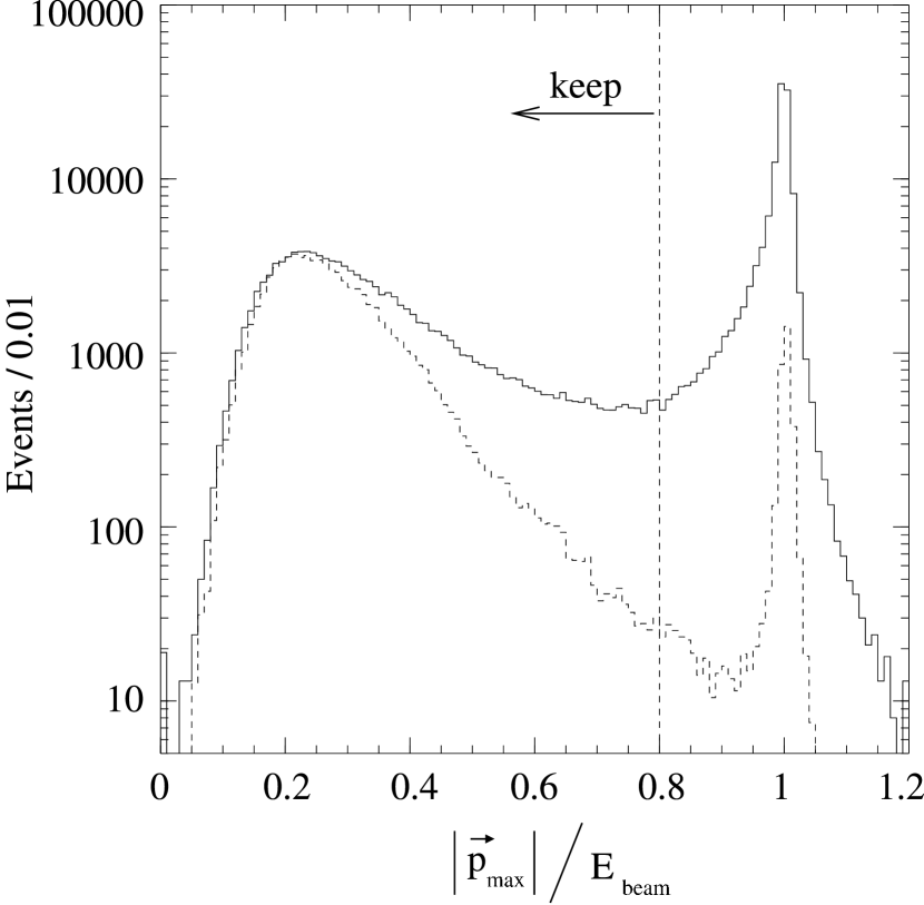
Figure 4.1: Largest track momentum ($|\vec{p}_{\mbox{\scriptsize max}}|$) in each event for data (solid histogram) and Monte Carlo $\Upsilon$ decays (dashed), with all other cuts applied. Data have large backgrounds from Bhabhas and radiative Bhabhas. Hadronic $\Upsilon$ decays peak at 20% of $E_{\mbox{\scriptsize beam}}$, while $\Upsilon\to e^{+}e^{-}$ and $\mu^{+}\mu^{-}$ peak at 100% of $E_{\mbox{\scriptsize beam}}$.

It is also common to reject Bhabhas by requiring more than two tracks in the event: according to our simulation, 98.9% of hadronic events have more than two tracks and 99.4% of Bhabhas in the observable range have exactly two. We considered this cut at an early stage in the analysis, but decided against it because we found the number of tracks distribution difficult to simulate for hadronic events. At that time, we intended to determine the cut efficiency with our Monte Carlo simulation, so this would have contributed significantly to the systematic uncertainty. Since then, we have found a way to measure hadronic efficiency without resorting to simulations, but we did not re-introduce the cut because we do not need it. The $|\vec{p}_{\mbox{\scriptsize max}}|$ cut reduces Bhabha contamination to approximately the same level as continuum $q\bar{q}$, so the Bhabha contribution to the statistical uncertainty of the background-subtracted count is not dominant. (Several of our cuts imply that an event must generate at least one track, but this does not significantly affect the Bhabha background.)

As previously mentioned, the cross-section of all continuum $e^{+}e^{-}\to f\bar{f}$ processes ($f$ is any fermion) fall off as $1/s$ while the two-photon fusion cross-section ($e^{+}e^{-}\to e^{+}e^{-}X$) increases as $\log s$. Continuum $f\bar{f}$ may therefore be estimated and subtracted collectively, while two-photon fusion must be handled separately, possibly introducing systematic error if it is large. We therefore suppress two-photon fusion events by requiring the visible energy of the event, $E_{\mbox{\scriptsize vis}}$, to be greater than 40% of $E_{\mbox{\scriptsize CM}}$. Visible energy is the sum of all track energies (determined from momentum, assuming the charged particle to have a mass of 140 MeV) and neutral shower energies (neutral showers must be at least 7 cm from all tracks). If all particles in an event are detected, $E_{\mbox{\scriptsize vis}}$ $\approx$ $E_{\mbox{\scriptsize CM}}$. As seen in Figure 4.2, hadronic $\Upsilon$ events peak in $E_{\mbox{\scriptsize vis}}$ at 80% $E_{\mbox{\scriptsize CM}}$, and there is a peak of non-$\Upsilon$ events at 15% $E_{\mbox{\scriptsize CM}}$. At least two-thirds of the events in this low-$E_{\mbox{\scriptsize vis}}$ peak are two-photon collisions, in which one incident electron has taken most of the center-of-mass energy, undetected, down the beam-pipe. We know this because two-thirds of events with less than 30% visible energy contain one low-momentum electron, whose charge and direction are correlated with the incident beams, and a highly anisotropic distribution of shower energy, presumably from the boosted hadron system $X$. Decays of $\tau^{+}\tau^{-}$ cover a broad spectrum of $E_{\mbox{\scriptsize vis}}$, due to energy lost in one or two neutrinos, extending but not peaking below our cut threshold.

Figure 4.2: Total visible energy ($E_{\mbox{\scriptsize vis}}$) in each event for data (solid histogram) and Monte Carlo $\Upsilon$ decays (dashed) with all other cuts applied. At least two-thirds of the peak at 15% of $E_{\mbox{\scriptsize CM}}$ in data are two-photon fusion events, and the peak above 50% of $E_{\mbox{\scriptsize CM}}$ are likely to be radiative Bhabhas, missing an electron. See text for a more complete discussion.

Rejecting low-$E_{\mbox{\scriptsize vis}}$ events also protects our hadron count from uncertainties associated with trigger thresholds. In our simulations, only 0.07% of hadronic events with $E_{\mbox{\scriptsize vis}}$ $>$ 40% $E_{\mbox{\scriptsize CM}}$ fail to trigger, so any fluctuations in the electronics will be on this level. The $E_{\mbox{\scriptsize vis}}$ threshold, situated in the flat minimum between the two-photon peak and the signal peak, is minimally sensitive to fluctuations in the two-photon background and the signal efficiency. Since only 0.82% of simulated hadronic $\Upsilon$ decays fail this cut, any fluctuations in this efficiency will be well under a percent.

In addition to the two-photon peak at an $E_{\mbox{\scriptsize vis}}$ of 20% $E_{\mbox{\scriptsize CM}}$, there is an excess of events with $E_{\mbox{\scriptsize vis}}$ just above 50% $E_{\mbox{\scriptsize CM}}$ (Figure 4.2). These events are likely to be radiative Bhabhas ($e^{+}e^{-}\to\gamma e^{+}e^{-}$) in which one of the two electrons is lost. They contain neutral calorimeter energy and an energetic electron whose charge and direction is correlated with the incident beams, like the two-photon fusion events. However, visible energy in two-photon collisions is expected to be much less than 50% of $E_{\mbox{\scriptsize CM}}$.

The number of background events from a continuum process is proportional to the integrated luminosity, just like the number of signal $\Upsilon$ decays. Their contribution to the apparent cross-section will therefore be purely a function of $E_{\mbox{\scriptsize CM}}$. The same cannot be said for backgrounds that are not the product of beam-beam collisions. Beam-gas and beam-wall rates are a function of the individual beam currents, the gas pressure inside the beam-pipe (for beam-gas) and the extreme tails of the bunch shape (for beam-wall). Cosmic rays are abundant in our detector, and the number of cosmic ray events is only a function of time. Integrated luminosity, integrated current, and time are approximately proportional (within a factor of two), so a continuum subtraction largely removes these effects, but not entirely.

We suppress beam-gas, beam-wall, and cosmic ray events by requiring the event to originate near the beam-beam crossing point. To select events originating near this point in an $x$-$y$ projection, we require at least one track to extrapolate within 5 mm of the beam-line. We define $d_{\mbox{\scriptsize XY}}$ as the distance of closest approach of the closest track to the beam-line, and reject events with $d_{\mbox{\scriptsize XY}}$ $>$ 5 mm. Tracks extrapolated from the tracking volume are corrected for momentum loss in the beam-pipe and silicon detector, and the location of the beam-beam crossing point is measured independently for each run, using the first 500 hadronic events. The $d_{\mbox{\scriptsize XY}}$ distribution (Figure 4.3) is much narrower than our 5 mm threshold: only 0.1% of beam-beam collision events fail this cut. This allows for $\sim$1 mm errors in the beam-beam intersection measurement, which is far larger than expected.

Figure 4.3: Distance from the closest track projection to the beam-line for data (solid histogram) and Monte Carlo $\Upsilon$ decays (dashed) with all other cuts applied. The sign is related to the orientation of the track’s curvature. The flat background in data is due to cosmic rays.

Our $d_{\mbox{\scriptsize XY}}$ cut is extremely effective at rejecting cosmic ray events. Cosmic rays rain uniformly into the detector, generating a uniform background to $d_{\mbox{\scriptsize XY}}$, which extends to 25 cm with our triggers. Only cosmic rays that pass within 5 mm of the beam-line survive. In principle, beam-wall events should also be eliminated, since they are generated in the beam-pipe, 2.1 cm from the beam-line. However, beam-wall events contain several tracks, any one of which may project into the accepted $d_{\mbox{\scriptsize XY}}$ region (Figure 4.4). By placing our requirement on the closest track, we bias this background to peak within our accepted region, diluting the effectiveness of the cut.

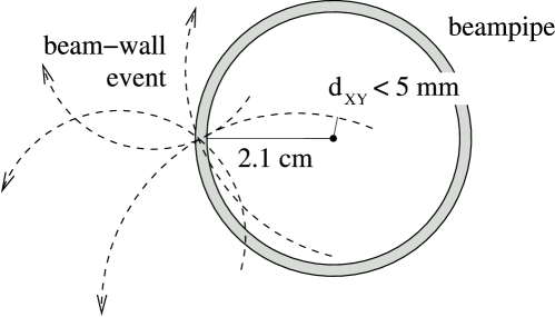
Figure 4.4: Though beam-wall events are centered at the beam-pipe, tracks may still project within 5 mm of the beam-line, thus passing the $d_{\mbox{\scriptsize XY}}$ cut.

Beam-gas and beam-wall events originate along the beam-line and beam-pipe, extending beyond beam-beam collisions in $z$. Placing a requirement on the closest track to the $z$-collision point would be ineffective for the same reason as above; beam-gas and beam-wall events both have many tracks, and the probability that one of these would project into the signal region (which is several centimeters wide) is not negligible. Instead, we reconstruct the $z$ position of the event vertex using all tracks, and call this quantity $d_{\mbox{\scriptsize Z}}$. The CLEO event vertexing algorithm is not useful because it was designed for signal reconstruction and fails to fit too many beam-gas and beam-wall events. Instead, we developed a simple algorithm of our own. Tracking resolution is such that most of the tracks from a beam-beam collision intersect within 0.1 mm of a common origin in the $x$-$y$ plane, and the number of intersections near this point grows rapidly with the number of primary tracks. Accidental track intersections far from this point grow more slowly. We can therefore determine the event vertex very accurately by averaging the $z$ positions of track-track intersections. We define the $z$ position of an $x$-$y$ intersection to be halfway between the $z$ positions of the two track helices, evaluated at the $x$-$y$ intersection point. If the intersection is a true three-dimensional vertex, the tracks’ $z$ positions will be nearly equal. We weight these intersections with uncertainties propagated from the track uncertainties, the tracks’ $z$ separation, and the $x$-$y$ distance to the beam-line added in quadrature, to prefer true intersections from the primary vertex. We plot this $d_{\mbox{\scriptsize Z}}$ distribution in Figure 4.5, and cut very loosely at 7.5 cm, to allow for errors in the beam-beam intersection measurement.

Figure 4.5: Location of the event vertex in $z$, according to our algorithm, for data (solid histogram) and Monte Carlo $\Upsilon$ decays (dashed) with all other cuts applied. Data and Monte Carlo differ in the $z$-length of the beam-beam overlap region. The flat background in data is primarily beam-gas and beam-wall, though Monte Carlo indicates that 0.5% of $\Upsilon$ decays are misreconstructed and extend beyond the cut threshold.

It is also possible to use track intersections to distinguish beam-wall events from beam-gas. The distance of the closest track-track intersection to the beam-line will be nearly zero for beam-gas events, but peak below the beam-pipe radius for beam-wall events (because selecting the closest intersection to the beam-line biases the distribution toward zero). In Figure 4.6, we plot the distribution of closest intersections for events with $d_{\mbox{\scriptsize XY}}$ $<$ 5 mm from data with only one beam in CESR. We see that the $d_{\mbox{\scriptsize XY}}$ cut reduces beam-wall to the extent that it is approximately as common as beam-gas. A more sophisticated average of intersections could help to discriminate between beam-gas and beam-wall, but as we will see in Subsection 4.3.4, the two processes combined are a small contamination, about 0.2% of the continuum for most runs. We therefore will not attempt to correct for beam-wall and beam-gas separately.

Figure 4.6: Closest track-track intersection to the beam-line in special data with one, non-colliding beam in CESR (all events are beam-gas, beam-wall, and cosmic rays). The rough peak below 0.6 cm is mostly beam-gas, and the broad peak from 1 to 2 cm is due to beam-wall events.

4.2 Data Quality Requirements

Not all data were collected under ideal conditions, so we applied some general criteria for rejecting bad runs. As the data were collected, two CLEO operators inspected the data for hardware failure. In the most serious cases, these data were eliminated from all CLEO analyses, but if the effect was limited, it was listed in a “bad runs” file (/home/dlk/Luminosity/badruns3S). We rejected any runs that were flagged with drift chamber, silicon vertex detector, or CsI calorimeter problems.

We want a robust measurement of cross-section, and cross-section is constant with time, even as the beam currents are depleted during a run. We therefore checked for variations in cross-section during each run by comparing hadronic events and $\gamma\gamma$ events in hundredths of each run. This ratio fluctuates statistically, but we found two examples in which the drift chamber lost sensitivity to tracks before the calorimeter lost sensitivity to showers in the last few minutes of the run (Figure 4.7). Most likely, the drift chamber lost high voltage just before the end of the run.

Figure 4.7: Ratio of hadronic events to $\gamma\gamma$ events as a function of time through two runs. The hadronic cross-section drops to zero in the last 3% of these runs (the dashed lines are linear fits to the data.)

To catch more instances of this kind of failure, we also compared the rate of trackless Bhabhas to total Bhabhas. We recognize the $e^{+}e^{-}$ final state by the two beam-energy showers it produces in the calorimeter, curved 0.1 radians away from perfect collinearity by the magnetic field. Twenty-five runs had high trackless Bhabha rates (above 0.3%), and all of the trackless Bhabha excesses were in the same hundredth of a run (usually the last). Ten of these (presented in Figure 4.8) were crucial to the resonance scans and therefore not rejected. Instead, we determined the cross-section from the first 99% of these runs. The twenty-seven runs with drift chamber failures are listed in Table 4.1.

Figure 4.8: Bhabha events with no observed tracks as a function of time through ten runs. In all of these cases, there is an excess in the last 1% of the run.

Table 4.1: Runs rejected for hardware/calibration reasons.

Drift chamber failed at the end of the run	121476, 121748, 121822, 121847, 122685, 123281, 123411, 123436, 123847, 123873, 124816, 124860, 124862, 125367, 126273, 126329, 127280
barrel-bhabha trigger inefficiency	121928, 121929, 121953, 127951, 127955, 130278, 121710, 121930, 121944, 121954, 123884
Overestimated track momenta	124452, 124454, 124456, 124458, 124462, 124464, 124465, 124466, 124467, 124469, 124472, 124473, 124474, 124475, 124477, 124478, 124479, 124480
Overestimated barrel shower energies	122331, 122335, 122336, 122339, 122341, 122342, 122344, 122345, 122349, 122350, 122352
Large cosmic ray/beam-gas backgrounds	122353, 126341, 129522
Large, unidentified backgrounds	121595, 122093, 122330, 126510
Too little data for tests	123013, 123014

The $\gamma\gamma$ final state, which we use for some diagnostic checks, is accepted only by the specialized barrel-bhabha trigger. We studied the efficiency of this trigger with Bhabha events and discovered eleven runs with very low efficiency, which we rejected, though these failures would only have affected our cross-checks. They are also listed in Table 4.1.

We also tested the quality of the drift chamber and calorimeter output by counting unphysically high-energy tracks and showers. In good data, less than 1% of Bhabhas will generate a track or a shower with momentum or energy above 120% $E_{\mbox{\scriptsize beam}}$. In a contiguous block of data on March 7, 2002, the fraction of high-momentum tracks abruptly increased to 3%. We see that the Bhabha peak for these runs has a high-energy tail (Figure 4.9), which suggests that the momentum in a fraction of tracks is overestimated. If this hypothesis applies to tracks with lower momenta, events may fail the $|\vec{p}_{\mbox{\scriptsize max}}|$ cut due to anomalous momentum measurements, changing the cut efficiency. We exclude these runs. On a separate occasion, December 16, 2001, the rate of high-energy showers abruptly rose to 3%. In this case, we observed that most of the unphysical showers occupy a regular block in the calorimeter barrel, indicating a read-out issue (Figure 4.10). Only our $E_{\mbox{\scriptsize vis}}$ cut depends on shower energies, and in particular, only showers that cannot be associated with any track, so the influence of calorimeter malfunctions on our hadronic efficiency is limited. However, we will use showers in the calorimeter barrel to identify Bhabhas and $\gamma\gamma$ events, so we exclude these runs as well. Another calorimeter malfunction, this time in the endcap, occured on December 25–29, 2001. The $E_{\mbox{\scriptsize vis}}$ spectrum for off-resonance runs in this time period is not distorted by excess background from a high-side tail on the two-photon fusion peak (see Figure 4.11), so we do not exclude these runs. All rejected runs are listed in Table 4.1.

Figure 4.9: The largest track momentum in off-resonance $\Upsilon(1S)$ (solid histogram) and March 7, 2002 runs (points with errorbars).

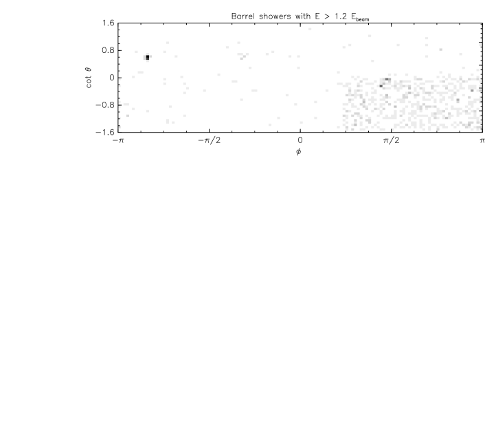
Figure 4.10: The locations of unphysical shower energies on December 16, 2001.

Figure 4.11: The visible energy spectrum in off-resonance $\Upsilon(3S)$ (solid histogram) and December 25–29, 2001 runs (points with errorbars).

We rejected a handful of runs due to high background rates. From Figure 4.19, we set a 5% upper limit on acceptable cosmic ray yields relative to the continuum yield, and an upper limit of 2% on beam-gas. Three runs failed these criteria. We also noticed that the fractions of hadronic, Bhabha, $\gamma\gamma$, and $\mu^{+}\mu^{-}$ events dropped abruptly in the middles of four runs, indicating a sudden turn-on of some large background. We rejected these, too. Finally, two runs had so little data (16,695 events total) that it was difficult to perform any of the above tests. We rejected them for convenience.

This analysis combines small “scan” datasets, taken on the $\Upsilon$ resonances but not at its maximum, with off-resonance and “peak” data taken at the maximum cross-sections. The scan data were acquired specifically for this analysis and therefore were not rejected lightly. (Only one run in Table 4.1 is a scan run: 124452.) The peak data are less valuable, and even after the selections described above, far more is available than is necessary. A measurement of the area of an $\Upsilon$ lineshape (i.e. $\Gamma_{ee}$) can be conceptually decomposed into width measurements and height measurements, in which the fractional uncertainty in the area is the sum of the fractional uncertainty in the width and in the height, in quadrature. Scan data constrain both the width and the height, while peak data constrain only the height. Adding peak data to a fit will always reduce the statistical uncertainty, though this reaches an asymptotic limit as the uncertainty comes to be dominated by the width measurements. However, as the beam energy calibration drifts with time, cross-sections slightly off the peak of the resonance may be represented as being exactly on-resonance, thereby biasing the height measurement. We accepted no more peak data than what is necessary to bring the statistical uncertainties within 5% of their limiting values. Since we are concerned with potential drifts with time, we re-expressed this limit as a time limit: we only include peak data in a lineshape fit if this data were taken less than 48 hours after the beginning of a scan. We imposed no limit on off-resonance data.

We rejected a $\Upsilon(1S)$ scan, acquired on April 3, 2002. This scan is missing key cross-section measurements on the high-energy side of the peak (Figure 4.12), which makes it difficult to assess uncertainties in the beam energy and the beam energy spread. This scan does include cross-section measurements well above the $\Upsilon$ mass, and may have been the victim of miscommunicated beam energy requests. (Requests are made relative to the $\Upsilon$ mass, and single-beam energies used by CESR differ from our center-of-mass energies by a factor of two.) Its exclusion from the $\Upsilon(1S)$ fit affects the fit result by 0.12% with no appreciable difference in uncertainty.

Figure 4.12: The April 3, 2002 lineshape scan, overlaid by a fit to all other $\Upsilon(1S)$ scans. No data significantly constrain the high-energy side of the peak.

4.3 Subtracting Residual Backgrounds

Backgrounds remaining after our cuts are summarized in Figure 4.13. We will discuss each of these, and their subtractions, in the subsections that follow.

Figure 4.13: The $\Upsilon(3S)$ lineshape in log scale, to illustrate backgrounds. The top dashed curve represents the sum of all backgrounds, which is dominated by $1/s$ continuum processes. The solid curves and data points below this are non-$1/s$ corrections included in “all backgrounds.” Dashed curves represent ISR tails from charmonium resonances which are included in the two-photon fusion curve. The overlap of ISR tail curves and non-beam-beam counts is accidental.

4.3.1 Backgrounds that Vary Slowly with Beam Energy

After our cuts, radiative Bhabhas and continuum $q\bar{q}$ dominate the background, adding a flat, 8 nb plateau below our three $\Upsilon$ peaks (18 nb, 7 nb, and 4 nb, respectively) in apparent cross-section versus $E_{\mbox{\scriptsize CM}}$. All continuum processes except for two-photon fusion evolve as $1/s$, so we include such a function in our lineshape fits. The magnitude of this term is determined independently for the $\Upsilon(1S)$, $\Upsilon(2S)$, and $\Upsilon(3S)$ by the large off-resonance samples taken only 20 MeV below each $\Upsilon$ mass. The $1/s$ curve is the dashed line near the top of Figure 4.13.

The first correction to the background curve is to add lower-energy $\Upsilon$ resonances, which have a $1/(\sqrt{s}-M_{\Upsilon})$ distribution. The magnitude of an ISR tail is set by the magnitude of the $\Upsilon$ resonance. We therefore fit $\Upsilon(1S)$, $\Upsilon(2S)$, and $\Upsilon(3S)$ in ascending order to obtain tail corrections from the previous fits. The $\Upsilon(1S)$ and $\Upsilon(2S)$ ISR tails under the $\Upsilon(3S)$ peak are labeled in Figure 4.13, and Figure 4.14 shows $\Upsilon(2S)$ and $\Upsilon(3S)$ off-resonance cross-sections with and without this tail correction.

Figure 4.14: Off-resonance cross-section measurements versus $E_{\mbox{\scriptsize CM}}$, with and without ISR tail corrections. (Corrected data are at the centers of the circles.) The solid curve is the best fit to $A/s+B\log s$, and the dashed curve is $1/s$ only, constrained to pass through the first data point.

To parameterize the $\log s$ correction for residual two-photon fusion, we fit the three off-resonance cross-sections to $A/s+B\log s$ and present this fit in Figure 4.15. We find (8.0 $\pm$ 0.5)% of the apparent cross-section at 9 GeV to be due to the $\log s$ component. To see if this is plausible, we roughly estimate the two-photon background surviving our cuts by extrapolating the two-photon peak above our cut threshold in $E_{\mbox{\scriptsize vis}}$ (see Figure 4.15), yielding a two-photon fraction of 6%. This is consistent with our $A/s+B\log s$ fit. Other effects may contribute to part of the $\log s$ term, such as $E_{\mbox{\scriptsize CM}}$ dependence in our cut efficiency for continuum events, a slow variation in the hadronic continuum cross-section, and ISR tails from charmonium resonances ($J/\psi$ and $\psi^{\prime}$, see Figure 4.13 for scale). All of these effects vary slowly with $E_{\mbox{\scriptsize CM}}$, so our parameterization for large differences in $E_{\mbox{\scriptsize CM}}$ (900 MeV from $\Upsilon(1S)$ to $\Upsilon(3S)$) applies to small differences in $E_{\mbox{\scriptsize CM}}$ as we project the $\Upsilon(1S)$, $\Upsilon(2S)$, and $\Upsilon(3S)$ off-resonance cross-sections below each peak. The difference in cross-section between a pure $1/s$ curve and the fully parameterized curve is only 0.04% at the peak.

Figure 4.15: The visible energy ($E_{\mbox{\scriptsize vis}}$) of off-resonance data, overlaid with a fit to the low-$E_{\mbox{\scriptsize vis}}$ peak. The fit is Gaussian on the low-energy side and Lorentzian on the high-energy side, and is used to roughly estimate the two-photon fusion events which survive after the 40% of $E_{\mbox{\scriptsize CM}}$ cut (dashed vertical line).

4.3.2 Continuum-Resonance Interference

As discussed in Section 2.3, resonant $\Upsilon\to q\bar{q}$ interferes with continuum $q\bar{q}$. We must therefore also add a $\tilde{\sigma}_{\mbox{\scriptsize int}}(E_{\mbox{\scriptsize CM}})$ term to our fit function (see Equation 2.8).

In this analysis, we assume that $e^{+}e^{-}\to q\bar{q}\to$ hadrons interferes with $e^{+}e^{-}\to\Upsilon\to q\bar{q}\to$ hadrons but not $e^{+}e^{-}\to\Upsilon\to ggg\to$ hadrons, though the latter may share some final states which are indistinguishable from $q\bar{q}$ decays. (Interference from $gg\gamma$ is negligible because its branching fraction is only 3% of $ggg$ and most $gg\gamma$ events have a distinctive, high-energy photon.) For interference between $q\bar{q}$ and $ggg$ decays, quantum states must remain coherent through the hadronization process. This effect has been observed in $J/\psi$ and $\psi^{\prime}\to\pi^{+}\pi^{-}$ and $K^{+}K^{-}$, but it is unclear if the effect is significant when summed over all final state amplitudes, since they may cancel. The phase difference between $q\bar{q}$ and $ggg$ for the inclusive process is also unknown, and some phase differences cannot be constrained by our lineshape fits. We will therefore only assume parton-level interference, and discuss full hadronic interference as a fitting issue in Chapter 8.

4.3.3 Backgrounds from $\Upsilon$

Since we are selecting hadronic $\Upsilon$ events, $\Upsilon\to e^{+}e^{-}$, $\mu^{+}\mu^{-}$, and $\tau^{+}\tau^{-}$ are backgrounds which peak under the hadronic $\Upsilon$ signal. We have no control sample for leptonic $\Upsilon$ modes, so we estimate these with a Monte Carlo simulation: negligible $e^{+}e^{-}$ and $\mu^{+}\mu^{-}$ survive the $|\vec{p}_{\mbox{\scriptsize max}}|$ cut (0.22% and 0.25%), even with final-state radiation ($\Upsilon\to\gamma e^{+}e^{-}$ and $\gamma\mu^{+}\mu^{-}$) modeled by PHOTOS. Our cuts and trigger are 57% efficient for $\tau^{+}\tau^{-}$, however. A tau lepton may decay into several hadrons, making it difficult to distinguish from hadronic $\Upsilon$ decays. Tau-pairs are rejected primarily by the $E_{\mbox{\scriptsize vis}}$ cut, as their visible energy spectrum is very broad due to neutrinos in the final state.

We will need to subtract $\tau^{+}\tau^{-}$ events from the hadronic $\Upsilon$ count. The $E_{\mbox{\scriptsize CM}}$ dependence of $\Upsilon\to\tau^{+}\tau^{-}$ is the same as $\Upsilon\to$ hadronic, though the magnitudes of the resonant and interference terms both differ. The resonant $\tau^{+}\tau^{-}$ contribution is a factor of ${\mathcal{B}}_{\tau\tau}/{\mathcal{B}}_{\mbox{\scriptsize had}}$ times smaller than the hadonic resonance, and the $\tau^{+}\tau^{-}$ interference term has a $\alpha_{\mbox{\scriptsize int}}$ of 0.20, 0.37, and 0.27 for the $\Upsilon(1S)$, $\Upsilon(2S)$, and $\Upsilon(3S)$, respectively. Continuum $\tau^{+}\tau^{-}$, like continuum $q\bar{q}$, is included in the $1/s$ term. When we estimate systematic uncertainties in the lineshape parameterization in Section 8.2 (page 8.2), we will note that the uncertainty in ${\mathcal{B}}_{\tau\tau}$ overwhelms the uncertainty in $\tau^{+}\tau^{-}$ efficiency and $\tau^{+}\tau^{-}$ $\alpha_{\mbox{\scriptsize int}}$, so only the branching fraction uncertainty must be propagated.

4.3.4 Beam-Gas, Beam-Wall, and Cosmic Rays

The non-beam-beam backgrounds are not a strict function of integrated luminosity, so we will need to explicitly subtract them from the hadronic $\Upsilon$ count for each run. To do this, we identify cosmic ray events, beam-gas, and beam-wall events in every run with special cuts. We then use control samples containing only cosmic rays or cosmic rays, beam-gas, and beam-wall to determine how to relate the number of non-beam-beam backgrounds that we counted to the number that survive our hadronic cuts. We then subtract this excess.

To identify cosmic rays, we require the following.

• No track may project within 5 mm of the beamspot ($|d_{\mbox{\scriptsize XY}}|$ $>$ 5 mm).

• The event must contain at least two tracks, since our track reconstruction algorithm identifies the descending-radius part of the cosmic ray as one track and the ascending-radius part as another.

• The normalized dot product of the two largest track momenta ($\vec{p}_{1}\cdot\vec{p}_{2}/|\vec{p}_{1}||\vec{p}_{2}|$) must be less than -0.999 or greater than 0.999, since the angles of these two tracks differ only due to tracking resolution (though the orientation may be confused by hits with unexpected drift times).

• The total calorimeter energy must be less than 2 GeV, consistent with two minimally-ionizing muon showers, and

• $E_{\mbox{\scriptsize vis}}$ $>$ 4% of $E_{\mbox{\scriptsize CM}}$ for less sensitivity to trigger thresholds.

These cuts are, by design, much more efficient for cosmic rays than our hadronic cuts, but the number of identified cosmic rays and the number of cosmic rays contaminating our hadron count is proportional. To determine this constant of proportionality, we apply both sets of event selection criteria to a data sample acquired with no beams in CESR. (The no-beam runs are listed in Table 4.2.) Figure 4.16 superimposes cosmic ray candidates from this no-beam sample on cosmic ray candidates from a large beam-beam sample, indicating a clear separation between cosmic rays and beam-beam collisions in $d_{\mbox{\scriptsize XY}}$. We assume that all events in the no-beam dataset which pass our hadronic cuts are cosmic rays, so the desired constant is just a ratio of the cosmic ray count to the hadronic event count in this sample. The effective cross-section of cosmic rays are plotted with uncertainties in Figure 4.13.

Table 4.2: Run numbers for beam-gas, beam-wall, and cosmic ray control datasets.

no-beam	128706 128736 128741 128748
electron single-beam	126828 126920 126922
positron single-beam	126785

Figure 4.16: Distance from the beam-line ($|d_{XY}|$ in $\log x$-scale, where 1 = one meter) with all other cosmic ray cuts applied. Data with beam-beam collisions are the solid histogram with a peak at 0.0001 (0.1 mm) from collisions and 0.01 (10 cm) from cosmic rays. Data from the no-beam sample are the points with error bars, normalized to equal numbers of cosmic rays. The dashed vertical line is the cut boundary at 5 mm. Triggers fail to accept cosmic rays beyond 25 cm.

Beam-gas and beam-wall events are hard to distinguish from one another, but they are both small backgrounds which depend on the electron and positron beam currents. This dependence is not identical, since beam-gas rates are proportional to the gas pressure inside the beam-pipe while beam-wall is not. However, the contamination from beam-gas and beam-wall combined is typically 0.2% of the continuum. Furthermore, our beam-gas and beam-wall cuts have a small background from beam-beam data, meaning that our estimate is too large. Instead of subtracting all of this estimate, we inflate our uncertainty.

To identify beam-gas and beam-wall events (which we will call beam-nucleus), we require

• $|d_{\mbox{\scriptsize XY}}|$ $<$ 5 mm, $|d_{\mbox{\scriptsize Z}}|$ $>$ 7.5 cm,

• $|\vec{p}_{1}\cdot\vec{p}_{2}|/|\vec{p}_{1}||\vec{p}_{2}|$ $<$ 0.9 to further reject cosmic rays,

• at least two tracks, and $E_{\mbox{\scriptsize vis}}$ $>$ 4% of $E_{\mbox{\scriptsize CM}}$.

To distinguish between electron-induced beam-nucleus and positron-induced beam-nucleus events, we also cut on the net $z$-momentum of all tracks ($p_{z}^{\mbox{\scriptsize tr}}$). For a positron-induced event, we require $p_{z}^{\mbox{\scriptsize tr}}$ $>$ 10% of $E_{\mbox{\scriptsize beam}}$ because incident positron momentum is in the positive $z$ direction (see Figure 3.4). Electron-induced events must have $p_{z}^{\mbox{\scriptsize tr}}$ $<$ $-$10% of $E_{\mbox{\scriptsize beam}}$.

To relate the number of identified beam-nucleus events to the number that contaminate our hadronic event count, we employ data samples acquired with only one beam in CESR (also listed in Table 4.2). To use these samples, we must first subtract the cosmic rays using the technique described above. Figure 4.17 demonstrates the separation of electron- and positron-induced beam-nucleus by their net $z$-momenta. This Figure also indicates that a small fraction, perhaps 10%, of our beam-nucleus candidates are contaminated by beam-beam events, probably two-photon fusion with a misreconstructed $d_{\mbox{\scriptsize Z}}$. The potential for contamination is also evident in Figure 4.18. Therefore, a beam-nucleus correction in analogy with the cosmic ray correction would be an over-subtraction of about 10%. The beam-nucleus estimates are typically only 0.1% of the continuum (Figure 4.19), so we subtract 50% $\pm$ 50% of the electron- and positron-induced beam-nucleus estimates. The effective cross-section of beam-nucleus estimates are plotted near the bottom of Figure 4.13. The cosmic ray and beam-nucleus estimates for every run we used to determine $\Gamma_{ee}$ are plotted in Figure 4.19.

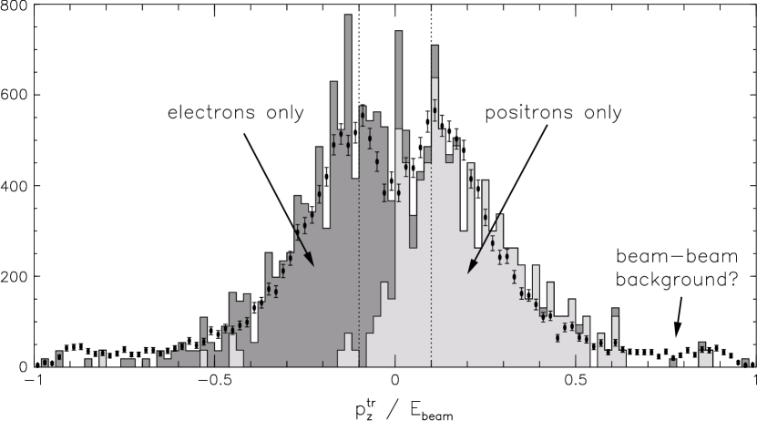
Figure 4.17: Net $z$-momentum of all tracks ($p_{z}^{\mbox{\scriptsize tr}}$) with all other beam-nucleus cuts applied. Data with only positrons in CESR are lightly-shaded, electrons-only are darkly-shaded and stacked on the positrons-only histogram, and data from collisions are represented by points with error bars. The boosts imparted by the incident beams are evident, and dotted vertical lines at $\pm$10% of $E_{\mbox{\scriptsize beam}}$ indicate cuts for electron- and positron-induced beam-nucleus events. The beam-beam data do not exactly reproduce the combined distribution, though the electrons-only and positrons-only histograms have been normalized to the same totals above and below $\pm$10% of $E_{\mbox{\scriptsize beam}}$.

Figure 4.18: Distance of the $z$ event vertex from the center of the beam-beam distribution ($|d_{Z}|$ in $\log x$-scale, where 1 = one meter). Data with beam-beam collisions are the solid histogram with a peak above the plot window at 0.01 (1 cm) from beam-beam collisions and a peak at 0.1 (10 cm) from beam-nucleus collisions. Data from the single-beam samples are the points with erorr bars, normalized to equal numbers of beam-nucleus events. Cosmic rays have been subtracted from both samples. The dashed vertical line is the cut boundary at 7.5 cm.

Figure 4.19: Total counts of non-beam-beam backgrounds as a fraction of the continuum level and a function of run number. Dashed vertical lines separate $\Upsilon(3S)$, $\Upsilon(1S)$, and $\Upsilon(2S)$ data-taking periods. Note that all three plots have different vertical scales: cosmic rays (a) are the most abundant, and the proportion of positron-induced beam-nucleus events (c) are typically twice that of electron-induced events (b).

Chapter 5 Hadronic Efficiency

5.1 Motivation for the Data-Based Approach

Inefficiency is in some sense the opposite of the problem of backgrounds: after removing the events which should not be in our hadronic $\Upsilon$ sample, we need to add in the events that are missing. In this Chapter, we will determine the probability that a hadronic $\Upsilon$ decay is included in our count, for each of the three resonances. These efficiencies are high, about 97% for each resonance.

Often, efficiencies are determined from Monte Carlo simulations. One simulates all known decay modes, and constructs an aggregate efficiency

$$\epsilon=\sum_{i}\,\epsilon_{i}\,{\mathcal{B}}_{i}\mbox{,}$$ (5.1)

where $\epsilon_{i}$ is the efficiency of each mode. We don’t directly use this method for two reasons.

1. Hadronic decays are the result of the hadronization of bare quarks and gluons. This is a non-perturbative process which is only empirically approximated by LUND/JetSet in the Monte Carlo. If we assume a non-perturbative QCD model to determine a non-perturbative QCD parameter, we would introduce a circular dependence that would have to be quantified.

2. Our definition of hadronic $\Upsilon$ decays includes potentially unknown modes whose efficiencies may be very different from the hadronic modes we simulate. For instance, it is possible that $\Upsilon$ decays into invisible wimps with zero efficiency or that unknown QCD resonances may enhance decays to $K_{L}$ or neutrons, which fail our $E_{\mbox{\scriptsize vis}}$ cut with greater probability.

Instead, we take advantage of our 1.3 fb^-1 sample of $\Upsilon(2S)$ decays to study $\Upsilon(2S)\to\pi^{+}\pi^{-}\Upsilon(1S)$ transitions. The $\Upsilon(1S)$ mesons in these decays are produced nearly at rest, and decay as they would from direct $e^{+}e^{-}\to\Upsilon(1S)$. However, the $2S\to 1S$ cascade events additionally include two charged pions which may satisfy a trigger and cause the event to be recorded, regardless of how the $\Upsilon(1S)$ decays. As an extreme example, we can use this technique to collect events featuring invisible $\Upsilon(1S)\to\nu\bar{\nu}$ or $\mbox{\sc wimp }\overline{\mbox{\sc wimp}}$ decays, which would be impossible with a direct $\Upsilon(1S)$ sample.

We exploit this broad access to $\Upsilon(1S)$ decays to measure the $\Upsilon(1S)$ efficiency. From $\Upsilon(2S)\to\pi^{+}\pi^{-}\Upsilon(1S)$ cascades, we select a subset in which the $\pi^{+}\pi^{-}$ by itself guarantees that the trigger will accept the event, so that we know that the trigger did not rely on decay products of the $\Upsilon(1S)$. Assuming that there is no correlation between the kinematics of the $\pi^{+}\pi^{-}$ and the branching fractions of the $\Upsilon(1S)$, this subset of $\pi^{+}\pi^{-}$ is accompanied by a generic set of $\Upsilon(1S)$ decays: $\Upsilon(1S)$ decay modes are represented in the data sample with the same proportions as in nature. We may then apply our cuts to the $\Upsilon(1S)$ decay products in our sample to determine the fraction which succeed. This is the efficiency.

5.2 Hadronic Efficiency of the $\Upsilon(1S)$

We have two goals for our event selection in this study, to identify $\Upsilon(2S)\to\pi^{+}\pi^{-}\Upsilon(1S)$ candidates and to choose $\pi^{+}\pi^{-}$ candidates which are sufficient to satisfy the trigger. The $\pi^{+}\pi^{-}$ in $\Upsilon(2S)\to\pi^{+}\pi^{-}\Upsilon(1S)$ are kinematically constrained by the mass difference between the $\Upsilon(2S)$ and the $\Upsilon(1S)$, so the mass of the system recoiling against the two pions,

$${m_{\mbox{\scriptsize$\pi\pi$-rec}}}^{2}=\left(M_{\Upsilon(2S)}-\sqrt{|\vec{p}_{1}|^{2}+{m_{\pi}}^{2}}-\sqrt{|\vec{p}_{2}|^{2}+{m_{\pi}}^{2}}\right)^{2}-|\vec{p}_{1}+\vec{p}_{2}|^{2}\mbox{,}$$ (5.2)

peaks at the $\Upsilon(1S)$ mass. This allows for excellent background rejection, because the peak from $\Upsilon(2S)\to\pi^{+}\pi^{-}\Upsilon(1S)$ has a 3 MeV resolution while the background spectrum is much broader (see Figure 5.1). We require $\pi^{+}\pi^{-}$ candidates to have a recoil mass ($m_{\mbox{\scriptsize$\pi\pi$-rec}}$) between 9.441 and 9.480 GeV. We further suppress background by requiring the track helices that we identify as $\pi^{+}\pi^{-}$ to intersect in the $x$-$y$ plane within 5 mm of the nominal beam-beam collision point. The track helices at this $x$-$y$ point must also be less than 2.5 cm from each other in $z$, and their average $z$ must be within 5 cm of the beam-beam collision point. The momenta used in Equation 5.2 are evaluated at the intersection point.

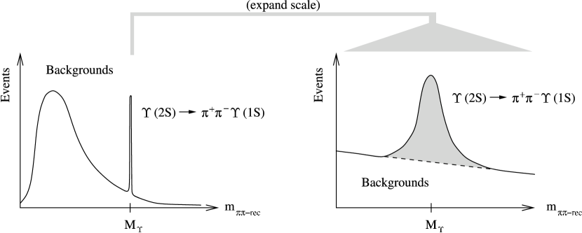
Figure 5.1: Distinguishing the recoil mass of $\pi^{+}\pi^{-}$ in kinematically-constrained $\Upsilon(2S)\to\pi^{+}\pi^{-}\Upsilon(1S)$ events from other, accidental track-track combinations (backgrounds). The background distribution is not simple, but it has no structure in the narrow region of our interest.

To satisfy the trigger, we select $\pi^{+}\pi^{-}$ track candidates with more than 150 MeV of momentum perpendicular to the $z$ axis ($p_{\perp}$), so that their trajectories reach beyond the sixteenth layer in the drift chamber and satisfy the geometric requirements for AXIAL tracks. A study of CLEO’s trigger response to hadronic tracks revealed that the probability for a track with $p_{\perp}$ $=$ 150 MeV to be detected as an AXIAL track is 99.96%, and this probability grows with $p_{\perp}$ [15]. We can therefore be at least 99.92% certain that events accepted by the two-track trigger (which requires two AXIAL tracks) with this cut on the $\pi^{+}\pi^{-}$ did not rely on $\Upsilon(1S)$ decay products to be accepted.

To simplify the process of excluding the $\pi^{+}\pi^{-}$ candidates when we apply our hadronic cuts, we additionally require each pion track to have more than 60 MeV of $z$-momentum magnitude. As discussed in Section 3.7 on page 3.7, such trajectories exit the detector before completing one half-orbit in the magnetic field. This protects our sample from events with pions which spiral in the tracking volume, potentially generating many tracks, only one of which is identified as a pion from $\Upsilon(2S)\to\pi^{+}\pi^{-}\Upsilon(1S)$. With this cut, we can assume that each pion is responsible for only one track and the calorimeter showers associated with that track.

There is occasionally more than one pair of tracks which satisfy these $\pi^{+}\pi^{-}$ criteria in a single event. In this case, we choose a $\pi^{+}\pi^{-}$ candidate randomly. If we were to choose the $\pi^{+}\pi^{-}$ candidate that best reconstructs the $\Upsilon(1S)$ mass, would bias the non-cascade background to peak under the $\Upsilon(2S)\to\pi^{+}\pi^{-}\Upsilon(1S)$ signal, complicating the background subtraction. Since the $\pi^{+}\pi^{-}$ candidate is chosen randomly, the background distribution has no structure on the scale of tens of MeV, and we can approximate it with a low-order polynomial.

Selecting $\Upsilon(2S)\to\pi^{+}\pi^{-}\Upsilon(1S)$ candidates in this manner, from events accepted by the two-track trigger, and applying our hadronic cuts to the $\Upsilon(1S)$ events in the peak, we find a hadronic $\Upsilon(1S)$ efficiency that is consistent with 100% with 3% uncertainty, which is not satisfactory for our analysis. Hadronic efficiency is a factor in $\Gamma_{ee}\Gamma_{\mbox{\scriptsize had}}/\Gamma_{\mbox{\scriptsize tot}}$, so the fractional uncertainty in hadronic efficiency adds to the $\Gamma_{ee}\Gamma_{\mbox{\scriptsize had}}/\Gamma_{\mbox{\scriptsize tot}}$ fractional uncertainty in quadrature.

The main culprit is the prescaled two-track trigger, which randomly rejects 94.7% of the events that satisfy its two AXIAL track criteria. We can circumvent this loss of data and improve the precision of our result by splitting the $\Upsilon(1S)$ hadronic efficiency into two factors. Define an $\Upsilon(1S)$ decay as “visible” if the trigger records one AXIAL track from the $\Upsilon(1S)$ decay products and one CBLO cluster from either the $\Upsilon(1S)$ decay or the $\pi^{+}\pi^{-}$. Define $\epsilon_{\mbox{\scriptsize vis}}$ to be the probability that an $\Upsilon(1S)$ decay is visible, and $\epsilon_{\mbox{\scriptsize cuts}}$ to be the probability that a visible $\Upsilon(1S)$ decay is selected by our triggers and cuts. The hadronic $\Upsilon(1S)$ efficiency is the product of $\epsilon_{\mbox{\scriptsize vis}}$ and $\epsilon_{\mbox{\scriptsize cuts}}$. We will determine $\epsilon_{\mbox{\scriptsize vis}}$, a number which is very close to 100%, using the two-track trigger, and $\epsilon_{\mbox{\scriptsize cuts}}$ using the hadron trigger, which selects visible $\Upsilon(1S)$ decays accompanied by $\pi^{+}\pi^{-}$. Since $(1-\epsilon_{\mbox{\scriptsize vis}})$ is such a small inefficiency, a large fractional uncertainty in $(1-\epsilon_{\mbox{\scriptsize vis}})$ propagates to a small fractional uncertainty in $\epsilon_{\mbox{\scriptsize vis}}$.

Our definition of “visible” is tailor-made for the hadron trigger in $\Upsilon(2S)\to\pi^{+}\pi^{-}\Upsilon(1S)$ events. The hadron trigger requires three AXIAL tracks and one CBLO cluster. We have selected $\pi^{+}\pi^{-}$ kinematics such that each pion must generate one AXIAL track, so the $\Upsilon(1S)$ decay is responsible for the third track and possibly the CBLO. Whatever the probability is that the CBLO comes from the $\pi^{+}\pi^{-}$, rather than the $\Upsilon(1S)$, it is the same while measuring $\epsilon_{\mbox{\scriptsize vis}}$ as it is while measuring $\epsilon_{\mbox{\scriptsize cuts}}$. This gives us the freedom to determine the cut efficiency with a large set of events from the hadron trigger, knowing that we can correct for the bias it introduces with $\epsilon_{\mbox{\scriptsize vis}}$.

In our article in Physical Review Letters [16], we discuss this technique more succinctly using two factors, $\epsilon_{\mbox{\scriptsize htrig}}$ and $\epsilon_{\mbox{\scriptsize cuts}}$. In that article, $\epsilon_{\mbox{\scriptsize htrig}}$ = $\epsilon_{\mbox{\scriptsize vis}}$, and $\epsilon_{\mbox{\scriptsize cuts}}$ has the same meaning in both.

5.2.1 Determination of $\epsilon_{\mbox{\scriptsize vis}}$

To determine $\epsilon_{\mbox{\scriptsize vis}}$, we apply the above procedure, replacing our full set of cuts for the “visible” condition we have just defined. The recoil mass distribution of $\pi^{+}\pi^{-}$ candidates accepted by the two-track trigger is shown in Figure 5.2(a). The real $\Upsilon(2S)\to\pi^{+}\pi^{-}\Upsilon(1S)$ events peak near the $\Upsilon(1S)$ mass of 9.46 GeV, and backgrounds are distributed linearly underneath. To measure the fraction of $\Upsilon(1S)$ decays that are “invisible,” we select from this sample events that fail the hadron trigger. These are plotted in Figure 5.2(b), revealing no significant peak. This indicates that nearly all of the $\Upsilon(1S)$ decays are visible.

Figure 5.2: Recoil mass of $\pi^{+}\pi^{-}$ candidates for (a) all events accepted by the two-track trigger, and (b) only those in which the rest of the event is “invisible.” True $\Upsilon(2S)\to\pi^{+}\pi^{-}\Upsilon(1S)$ events are contained in the peak near 9.46 GeV, which is highly suppressed in (b), indicating that very few $\Upsilon(1S)$ decays are invisible. The solid curve is a fit to the data, and the dashed curve is the linear background contribution.

To quantify this statement, we fit the data in Figures 5.2(a) and 5.2(b) to the same function and extract the ratio of $\Upsilon(2S)\to\pi^{+}\pi^{-}\Upsilon(1S)$ yields. We fit the full two-track dataset (Figure 5.2(a)) to a double Gaussian with a 1:4 ratio of areas and a linear background. When we fit the invisible-$\Upsilon(1S)$ data (Figure 5.2(b)), we fix the mean and widths, imposing the assumption that momentum resolution of the $\pi^{+}\pi^{-}$ is independent of the visibility of the $\Upsilon(1S)$. This very reasonable assumption purchases much of the statistical precision in the measurement. The ratio of fit yields, which is the probability that an $\Upsilon(1S)$ decay will be invisible, is (0.67 $\pm$ 0.62)%.

The invisible $\Upsilon\to\nu\bar{\nu}$ and $\Upsilon\to\mbox{\sc wimp}\overline{\mbox{\sc wimp}}$ we discussed earlier are included in $(1-\epsilon_{\mbox{\scriptsize vis}})$, though the 0.05% $\Upsilon\to\nu\bar{\nu}$ branching fraction is much smaller than the statistical uncertainty. This measurement does, however, place a model-independent upper bound on unknown, neutral decays of $\Upsilon(1S)$, which may be interesting for constraining models that feature new neutral particles such as wimps or large branching fractions for all-neutral hadronic events. This is a constraint on neutral decays because our definition of “visible” requires at least one track with $|\cos\theta|<0.93$ and $p_{\perp}>150$ MeV. The $\Upsilon(1S)$ branching fraction to events with no such tracks is less than 1.01% at 90% confidence level.

This ratio of fit yields represents the fraction of $\Upsilon(1S)$ decays that are invisible, including leptonic $\Upsilon(1S)$ decays. Leptonic decays, particularly $e^{+}e^{-}$ and $\mu^{+}\mu^{-}$, are more likely to be invisible than hadronic decays, since their final state consists of only two particles which are geometrically back-to-back: if one lepton disappears down the beam-pipe, the other probably will do so on the other side. We determine the probability for leptons to be invisible from leptonic Monte Carlo simulations (which include the $(1+\cos\theta)$ angular distribution for leptonic decays through a virtual photon), and this probability is (10.91 $\pm$ 0.01)%. We use Equation 5.1 to determine the hadronic visibility efficiency, $\epsilon_{\mbox{\scriptsize vis}}$, from the total visibility efficiency ($\epsilon_{\mbox{\scriptsize vis}}^{\mbox{\scriptsize tot}}=1-0.0067$) and the leptonic visibility efficiency ($\epsilon_{\mbox{\scriptsize vis}}^{\mbox{\scriptsize lep}}=1-0.1091$).

$$\epsilon_{\mbox{\scriptsize vis}}=\frac{\epsilon_{\mbox{\scriptsize vis}}^{\mbox{\scriptsize tot}}-\epsilon_{\mbox{\scriptsize vis}}^{\mbox{\scriptsize lep}}\times(3{\mathcal{B}}_{\mu\mu})}{(1-3{\mathcal{B}}_{\mu\mu})}=(100.02\pm 0.62)\%\mbox{.}$$ (5.3)

Slightly more than half of this probability distribution is above 100%, which is impossible for a real efficiency, so we truncate the part above 100% and normalize the remaining distribution to obtain an asymmetric uncertainty: $\epsilon_{\mbox{\scriptsize vis}}$ = (99.59 ${}^{+0.29}_{-0.45}$)%.

5.2.2 Determination of $\epsilon_{\mbox{\scriptsize cuts}}$

We select $\pi^{+}\pi^{-}$ candidates in the same way to determine $\epsilon_{\mbox{\scriptsize cuts}}$, except that we choose events accepted by the hadron trigger rather than the two-track trigger. Figure 5.3(a) presents the recoil mass of these $\pi^{+}\pi^{-}$ candidates, recoiling against visible $\Upsilon(1S)$ decays. We apply our hadronic cuts (but not the trigger requirements) to this sample, excluding tracks and showers associated with the $\pi^{+}\pi^{-}$, and plot the recoil mass for these in Figure 5.3(b). These “cut-failure” events have a prominent peak at the $\Upsilon(1S)$ mass due to all the visible $\Upsilon(1S)$ events which failed our cuts. (Most of them are leptonic decays.)

Figure 5.3: Recoil mass of $\pi^{+}\pi^{-}$ candidates for (a) all events accepted by the hadron trigger, and (b) only those in which the rest of the event fails our cuts (“cut-failure” events). The dotted vertical lines identify the signal region, and the dashed curve is a fit to the background, used to subtract background events from the signal region.

To obtain the ratio of cut-failure $\Upsilon(1S)$ events to all visible $\Upsilon(1S)$ events, we avoid the fit procedure because of the potential for systematic uncertainties in the fit parameterization. In the $\epsilon_{\mbox{\scriptsize vis}}$ study, the statistical uncertainty in the number of invisible events was almost as large as the number of invisible events itself, and this overwhelmed any bias introduced by the fit function shape. Here, the number of cut-failures is significantly greater than zero and ought to be measured more precisely. Instead of fitting, we count events with a recoil mass between 9.454 and 9.472 GeV and subtract the backgrounds, which have been determined by a linear fit to the sidebands (between 9.441 and 9.480 GeV, excluding the signal region). To estimate the systematic uncertainty in yield due to assuming a linear background, we repeat the procedure with the largest quadratic term allowed by the data.

The ratio of cut-failure $\Upsilon(1S)$ events to all visible $\Upsilon(1S)$ events is (92.58 $\pm$ 0.13 $\pm$ 0.02)%, where the first uncertainty is statistical and the second is due to the parameterization of the background distribution. The leptonic modes account for most of this 7% inefficiency: correcting for leptonic modes as above (Equation 5.3) yields $\epsilon_{\mbox{\scriptsize cuts}}$ = (98.32 $\pm$ 0.21)%.

The apparent $\Upsilon(1S)$ efficiency, measured in $\Upsilon(2S)\to\pi^{+}\pi^{-}\Upsilon(1S)$ cascades, may differ from the efficiency of direct $e^{+}e^{-}\to\Upsilon(1S)$ events because of the slight relativistic boost of the $\Upsilon(1S)$ ($\gamma=1.005$) or the potential for $\pi^{+}\pi^{-}$ showers to overlap $\Upsilon(1S)$ showers in cascade decays. To address these possibilities, we generate hadronic Monte Carlo for the direct and the cascade cases, applying the same procedure to determine the hadronic efficiency from the cascade simulation. We observe no significant difference: the ratio of direct efficiency to cascade efficiency is 1.0014 $\pm$ 0.0022. We apply this as a correction primarily to propagate the uncertainty in this study.

Incidentally, the cascade Monte Carlo prediction of $\epsilon_{\mbox{\scriptsize cuts}}$, (98.54 $\pm$ 0.22)%, agrees with our data-based measurement of (98.32 $\pm$ 0.21)%. We would have been correct, if not justified, if we had derived our cut efficiency directly from the Monte Carlo. We also extract $|\vec{p}_{\mbox{\scriptsize max}}|$, $E_{\mbox{\scriptsize vis}}$, $d_{\mbox{\scriptsize XY}}$, and $d_{\mbox{\scriptsize Z}}$ from our cascade data and cascade Monte Carlo, and find that they agree fairly well (Figure 5.4).

Figure 5.4: Our four cut variables, as seen in background-subtracted $\Upsilon(2S)\to\pi^{+}\pi^{-}\Upsilon(1S)$ events. Points with errorbars are data, the solid histograms are $\Upsilon(2S)\to\pi^{+}\pi^{-}\Upsilon(1S)$ Monte Carlo simulations with the same procedure applied, and the dotted vertical lines are the cut thresholds. (a) Largest track momentum ($|\vec{p}_{\mbox{\scriptsize max}}|$), divided by $M_{\Upsilon(1S)}/2$, the equivalent of $E_{\mbox{\scriptsize beam}}$ if this were a direct decay. The peak at 1 is due to $e^{+}e^{-}$ and $\mu^{+}\mu^{-}$ decays, cross-hatched in the Monte Carlo. (b) Visible energy ($E_{\mbox{\scriptsize vis}}$), divided by $M_{\Upsilon(1S)}$, the equivalent of $E_{\mbox{\scriptsize CM}}$. (c) The distance of the closest track to the beam-line ($d_{\mbox{\scriptsize XY}}$). (d) The $z$-vertex of the event ($d_{\mbox{\scriptsize Z}}$).

One correction is still missing from the $\epsilon_{\mbox{\scriptsize cuts}}$ we have derived: $\epsilon_{\mbox{\scriptsize cuts}}$ must include the trigger efficiency, but we excluded trigger requirements from our measurement. While we can remove the $\pi^{+}\pi^{-}$ tracks and showers from our fully reconstructed data, it would be impractical to apply an analogous procedure on our trigger data for technical reasons. We therefore use Monte Carlo to determine the efficiency of the trigger once our cuts have been applied, a value of 99.87%. Figure 5.5 overlays data and Monte Carlo AXIAL, STEREO, CBLO, and CBMD distributions in direct $\Upsilon(1S)$ decays, showing fairly good agreement. The predicted inefficiency of 0.13% can therefore be trusted within 100% of itself, so we conservatively assign this as the systematic uncertainty.

Figure 5.5: The four cut variables used in hadron, rad-tau, and $e^{\pm}$-track trigger decisions (defined on page • ‣ 3.2). Points with errobars are continuum-subtracted data, histograms are Monte Carlo simulations, and the dashed vertical lines are cut thresholds. Trigger selections have been applied to data and Monte Carlo, though Monte Carlo without trigger selections are overlaid as dotted histograms (barely visible).

After all of these corrections, the efficiency of visible hadronic $\Upsilon(1S)$ decays is $\epsilon_{\mbox{\scriptsize cuts}}$ = $(0.9832)(0.9987)(1.0014)$ = (98.33 $\pm$ 0.33)%. The efficiency of all hadronic $\Upsilon(1S)$ decays is $\epsilon_{\mbox{\scriptsize vis}}$ $\times$ $\epsilon_{\mbox{\scriptsize cuts}}$ = (97.93 ${}^{+0.44}_{-0.56}$)%.

5.3 Hadronic Efficiency of the $\Upsilon(2S)$ and $\Upsilon(3S)$

The $\Upsilon(3S)\to\pi^{+}\pi^{-}\Upsilon(2S)$ and $\Upsilon(4S)\to\pi^{+}\pi^{-}\Upsilon(3S)$ rates are too low to accumulate large samples to study $\Upsilon(2S)$ and $\Upsilon(3S)$ efficiencies in the same way that we did $\Upsilon(1S)$. Instead, we derive correction factors from the Monte Carlo that allow the $\Upsilon(1S)$ efficiency to be applied to the $\Upsilon(2S)$ and $\Upsilon(3S)$.

The decays of the $\Upsilon(2S)$ and $\Upsilon(3S)$ differ from those of the $\Upsilon(1S)$ in two ways. The $\Upsilon(2S)$ and $\Upsilon(3S)$ decay products are slightly more energetic, as they originate in a state of higher $E_{\mbox{\scriptsize CM}}$, and the $\Upsilon(2S)$ and $\Upsilon(3S)$ can decay via transitions to lower $b\bar{b}$ resonances. The first correction is very small because our $|\vec{p}_{\mbox{\scriptsize max}}|$ and $E_{\mbox{\scriptsize vis}}$ cut thesholds are constant fractions of $E_{\mbox{\scriptsize CM}}$, and the difference in $E_{\mbox{\scriptsize CM}}$ from $\Upsilon(1S)$ to $\Upsilon(3S)$ is only 10%. In the Monte Carlo simulation, the $\Upsilon(2S)$ and $\Upsilon(3S)$ efficiency for $ggg$, $gg\gamma$, and $q\bar{q}$ is only 0.2% lower than the $\Upsilon(1S)$ efficiency.

Most $\Upsilon(2S)$ and $\Upsilon(3S)$ transition decays have the same efficiency as $ggg$, $gg\gamma$, and $q\bar{q}$, so they have no impact on total hadronic efficiency. The exceptions are transitions that result in a lower $\Upsilon$ resonance decaying into $e^{+}e^{-}$ or $\mu^{+}\mu^{-}$. According to the Monte Carlo simulation, these “cascade-to-leptons” decays have (0.69 $\pm$ 0.22)% efficiency for $\Upsilon(2S)$ and (0.38 $\pm$ 0.19)% efficiency for the $\Upsilon(3S)$— almost zero. Therefore the efficiency correction will be approximately $(1-{\mathcal{B}}_{\mbox{\scriptsize cas}})$, where ${\mathcal{B}}_{\mbox{\scriptsize cas}}$ is the branching fraction for these modes.

We determine this branching fraction from the data by counting cascade-to-leptons events relative to $\Upsilon\to\mu\mu$ in the full $\Upsilon(2S)$ and $\Upsilon(3S)$ datasets. We select all events that have two high-momentum tracks ($|\vec{p}|>$ 70% $E_{\mbox{\scriptsize beam}}$) without associated high-energy showers ($E_{\mbox{\scriptsize max}}<$ 70% $E_{\mbox{\scriptsize beam}}$), that is, consistent with two high-energy muons accompanied by anything. We plot the invariant mass of these two muons in Figure 5.6, after subtracting continuum processes using the off-resonance data. Muon pairs from direct $\Upsilon$ decays are easily distinguished from cascade-to-leptons events. The Monte Carlo reproduces the invariant mass spectrum with only tiny errors in the calibration of the magnetic field (a horizontal shift in the plot).

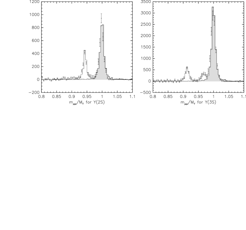
Figure 5.6: Invariant mass spectra of $\mu^{+}\mu^{-}$ in events with two energetic muons. Points with errorbars are continuum-subtracted data, and histograms are Monte Carlo simulations, with prompt $\Upsilon\to\mu^{+}\mu^{-}$ shaded. The horizontal shift in energy scale is consistent with the uncertainty in our magnetic field estimate.

We measure ${\mathcal{B}}_{\mbox{\scriptsize cas}}$ relative to ${\mathcal{B}}_{\mu\mu}$ by fitting Monte Carlo cascade-to-muon pairs and Monte Carlo direct muon pairs to the data in Figure 5.6. This fit has two free parameters, the magnitude of ${\mathcal{B}}_{\mbox{\scriptsize cas}}$ and the magnitude of ${\mathcal{B}}_{\mu\mu}$. We assign conservative 10% uncertainties to this procedure, which overwhelm ${\mathcal{B}}_{\mu\mu}$ uncertainties and yield only 0.1% uncertainties in the final efficiency determination. The resulting ${\mathcal{B}}_{\mbox{\scriptsize cas}}$ for $\Upsilon(2S)$ is (1.58 $\pm$ 0.16)% and for $\Upsilon(3S)$ is (1.34 $\pm$ 0.13)%, accounting for the factor of two from cascade-to-electron pairs.

Applying these corrections to the $\Upsilon(2S)$ and $\Upsilon(3S)$ efficiencies, we obtain (96.18 ${}^{+0.44}_{-0.56}$ $\pm$ 0.15)% and (96.41 ${}^{+0.44}_{-0.56}$ $\pm$ 0.13)% for the $\Upsilon(2S)$ and $\Upsilon(3S)$, respectively. The first uncertainty is derived from the $\Upsilon(2S)\to\pi^{+}\pi^{-}\Upsilon(1S)$ study and is common to all three resonances. The second uncertainty arises from our ${\mathcal{B}}_{\mbox{\scriptsize cas}}$ measurements and is independent for the $\Upsilon(2S)$ and $\Upsilon(3S)$. The first uncertainty therefore cancels in ratios of $\Gamma_{ee}$, while the second does not.

Chapter 6 Integrated Luminosity

Now that we can reliably count the number of hadronic $\Upsilon$ decays at every $E_{\mbox{\scriptsize CM}}$ we sampled, we need to determine the hadronic cross-section this implies by measuring the integrated luminosity of the same data. We get the integrated luminosity from a count of Bhabha events, since these are plentiful and their rate can be accurately calculated from perturbative QED. Integrated luminosity is the ratio of Bhabha events counted to the efficiency-weighted Bhabha cross-section, and the hadronic $\Upsilon$ cross-section is the ratio of hadronic $\Upsilon$ events to the integrated luminosity.

Any theoretically calculable process can be used to determine the integrated luminosity; Bhabhas were chosen primarily for their abundance, since this minimizes statistical uncertainty. A Bhabha count is complicated by the fact that $\Upsilon\to e^{+}e^{-}$ is indistinguishable from Bhabhas on an event-by-event basis, and this background peaks under the resonance. Alternatively, one could determine the integrated luminosity from $e^{+}e^{-}\to\gamma\gamma$ because $\Upsilon\not\to\gamma\gamma$ (Electromagnetic decays do not violate parity). Unfortunately, this comes at the cost of a factor of 8.6 in statistics. The $\Upsilon\to e^{+}e^{-}$ contribution can easily be controlled, and the additional statistical power is valuable when determining ratios of $\Gamma_{ee}$$(nS)$/$\Gamma_{ee}$$(mS)$, so we determine integrated luminosities from Bhabhas and use $\gamma\gamma$ events as a cross-check.

6.1 Bhabha Count and $\gamma\gamma$ count

To select Bhabha events, we require

• two or more tracks with momenta between 50% and 110% of $E_{\mbox{\scriptsize beam}}$, and an energy sum (including showers from bremsstrahlung radiation as the electrons propagate through the detector) of more than 90% $E_{\mbox{\scriptsize CM}}$.

• The larger (smaller) track $|\cos\theta|$ must be less than 0.766 (0.707), and

• each track must be associated with a calorimeter shower, with the larger (smaller) shower energy divided by track momentum ($E_{\mbox{\scriptsize shower}}/|\vec{p}_{\mbox{\scriptsize track}}|$) being greater than 80% (50%).

With these cuts, backgrounds other than $\Upsilon\to e^{+}e^{-}$ are negligible. Different thresholds are set for the larger and smaller angles and calorimeter energies to reduce sensitivity to the threshold values, and possible efficiency variation with time. See Figure 6.1 for an illustration of this kind of cut.

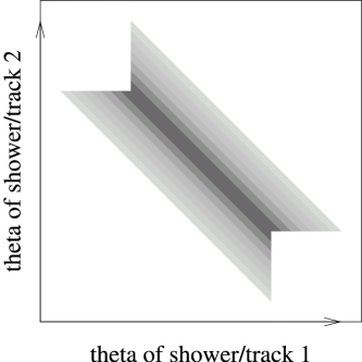
Figure 6.1: The distribution of two anti-correlated variables with an asymmetric cut (the masked square regions). Horizontal and vertical smearing around the central diagonal is independent; we cut each track or shower in a way that doesn’t imply a cut on the other.

Contamination from $\Upsilon\to e^{+}e^{-}$ at the resonance peaks is 3.8%, 1.4%, and 1.0%, respectively. This background is readily calculated for any $E_{\mbox{\scriptsize CM}}$ by multiplying the $\Upsilon$ lineshape by ${\mathcal{B}}_{ee}$ (we assume ${\mathcal{B}}_{ee}$ = ${\mathcal{B}}_{\mu\mu}$ for greater precision) and the cut efficiency for $\Upsilon\to e^{+}e^{-}$ (which has a different angular distribution than Bhabhas). Since the $\Upsilon$ lineshapes are derived from cross-section measurements, this is a circular dependence, so we applied an iterative procedure, starting with $\gamma\gamma$ luminosity. The $\Upsilon$ and continuum $e^{+}e^{-}$ interfere, so we also calculate an interference term (Equation 2.8) with $\alpha_{\mbox{\scriptsize int}}$ = 0.60, 0.87, and 0.69 for $\Upsilon(1S)$, $\Upsilon(2S)$, and $\Upsilon(3S)$, respectively. The effective cross-section for $e^{+}e^{-}$ as a function of $E_{\mbox{\scriptsize CM}}$, including the continuum and $\Upsilon$ contributions, is presented in Figure 6.2, with and without the interference term. The presence of the interference term has negligible impact on the lineshape fit results.

Figure 6.2: The influence of $\Upsilon\to e^{+}e^{-}$ on effective $e^{+}e^{-}$ cross-section, with interference (solid) and without interference (dashed). Note that the vertical axis is zero-suppressed.

To select $\gamma\gamma$ events for our cross-checks, we require

• two showers (subscripted 1 and 2) with energies higher than 70% of $E_{\mbox{\scriptsize beam}}$,

• $|\cot\theta_{1}+\cot\theta_{2}|<0.1$ (showers back-to-back in $\theta$, the polar angle), and

• $|\sin(\phi_{1}-\phi_{2})|<0.04$ (showers back-to-back in $\phi$, the azimuthal angle).

• The larger (smaller) $|\cot\theta|$ must be less than 1.28 (1.18) (this is within the calorimeter barrel),

• the larger (smaller) $|\cot\theta|$ must be greater than 0.15 (0.05) (avoiding the central region, where trigger efficiency is low), and

• there must be no tracks in the event.

When we select $\gamma\gamma$ events, we are dependent on only one trigger, barrel-bhabha, since this is the only trigger that doesn’t require any tracks. We studied the efficiency of this trigger with Bhabhas, and found calorimeter tiles whose efficiencies dropped for a significant fraction of the data-taking period. Rather than applying a run-dependent efficiency, we masked out these regions with our cuts. The largest shower on the western side of the detector must not be found in any of these regions:

• $-\frac{14}{64}\pi<\phi<\frac{9}{64}\pi$ and $|\cot\theta_{1}+\cot\theta_{2}|<1.08$,

• $-\frac{53}{64}\pi<\phi<-\frac{14}{64}\pi$ and $|\cot\theta_{1}+\cot\theta_{2}|>1.90$, and

• $-0.4<\phi<-0.3$.

Given these angular cuts, the barrel-bhabha trigger is 99.67% efficient with only statistical deviations. (The efficiency of every run is above 99.2%.)

6.2 Overall Luminosity Scale

The efficiency-weighted Bhabha cross-section is the second ingredient in the luminosity measurement. This sets the luminosity scale for all Bhabha counts. The scale factor, a number of nb^-1 per observed Bhabha, is the inverse of the efficiency-weighted Bhabha cross-section (nb).

The efficiency-weighted cross-section is the cross-section of observed Bhabhas. Expressed as an integral over a single variable for clarity,

$$\sigma_{\mbox{\scriptsize eff}}=\int_{0}^{\pi}\frac{d\sigma}{d\theta}\,\epsilon(\theta)\,d\theta$$ (6.1)

where $\epsilon(\theta)$ is our detector’s Bhabha cut efficiency at a given polar angle $\theta$. Rather than exhaustively simulating the detector’s response to Bhabhas in $\theta$ bins, we generate Bhabhas with an angular cut-off beyond the detector’s geometric acceptance (where $\epsilon(\theta)=0$), calculate the cross-section this represents ($\sigma_{0}$), and multiply it by the efficiency of these simulated events ($\epsilon_{0}$), determined by passing them through the detector simulation. Both $\sigma_{0}$ and $\epsilon_{0}$ depend on our choice of cut-off, but the product doesn’t. This product is the desired efficiency-weighted cross-section because

$$\sigma_{0}=\int_{\theta_{\mbox{\scriptsize min}}}^{\theta_{\mbox{\scriptsize max}}}\frac{d\sigma}{d\theta^{\prime}}\,d\theta^{\prime}\mbox{\hskip 14.22636pt and \hskip 14.22636pt}\epsilon_{0}=\int_{\theta_{\mbox{\scriptsize min}}}^{\theta_{\mbox{\scriptsize max}}}\frac{dP}{d\theta}\,\epsilon(\theta)\,d\theta\mbox{.}$$ (6.2)

where $dP/d\theta$ is the probability distribution of Bhabhas with polar angle $\theta$ in our simulation, which is normalized:

$$\frac{dP}{d\theta}=\left(\frac{d\sigma}{d\theta}\right)\left(\int_{\theta_{\mbox{\scriptsize min}}}^{\theta_{\mbox{\scriptsize max}}}\frac{d\sigma}{d\theta^{\prime}}\,d\theta^{\prime}\right)^{-1}_{\mbox{\normalsize.}}$$ (6.3)

Equation 6.1 may be derived from Equations 6.2 and 6.3.

We simulate Bhabhas with the Babayaga event generator, which calculates $dP/d\theta$ and $\sigma_{0}$ to fourth order in the fine structure constant [17], with an angular cut-off of $|\cos\theta_{\mbox{\scriptsize max}}|$ = 0.819. Passing these simulated events through our full detector simulation, we calculate an efficiency-weighted cross-section of 8.993 $\pm$ 0.035 nb^-1 at an $E_{\mbox{\scriptsize CM}}$ of 9.43 GeV, 7.945 $\pm$ 0.031 nb^-1 at 10.00 GeV, and 7.361 $\pm$ 0.032 nb^-1 at 10.33 GeV, which are the off-resonance $\Upsilon(1S)$, $\Upsilon(2S)$, and $\Upsilon(3S)$ energies, respectively.

The Monte Carlo reproduces data distributions well at all three energies, which is demonstrated for the 10.33 GeV data in eight relevant distributions in Figures 6.3–6.10.

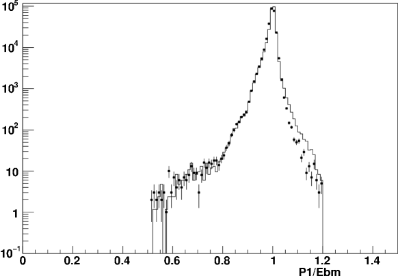
Figure 6.3: Largest track momentum divided by $E_{\mbox{\scriptsize beam}}$ in the 10.33 GeV data (points) and Monte Carlo (histogram) with other cuts applied. Data between 0.5 and 1.1 are accepted.

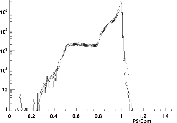
Figure 6.4: Second-largest track momentum divided by $E_{\mbox{\scriptsize beam}}$ in the 10.33 GeV data (points) and Monte Carlo (histogram) with other cuts applied. Data between 0.5 and 1.1 are accepted.

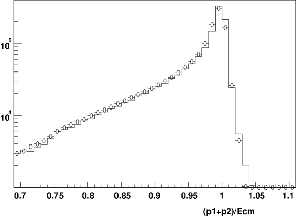
Figure 6.5: Sum of two largest-momentum track energies and associated bremsstrahlung showers divided by $E_{\mbox{\scriptsize CM}}$ in the 10.33 GeV data (points) and Monte Carlo (histogram) with other cuts applied. Data above 0.9 are accepted.

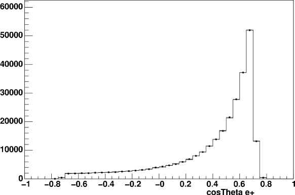
Figure 6.6: Positron $\cos\theta$ (polar angle) distribution in the 10.33 GeV data (points) and Monte Carlo (histogram) with other cuts applied. The larger (smaller) $|\cos\theta|$ of the two electrons must be below 0.766 (0.707) for acceptance.

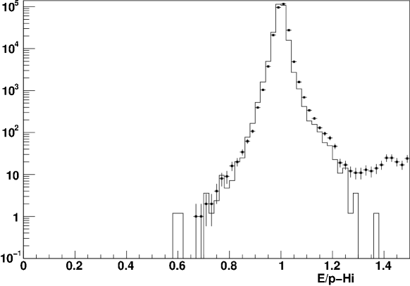
Figure 6.7: Largest $E_{\mbox{\scriptsize shower}}/|\vec{p}_{\mbox{\scriptsize track}}|$ divided by $E_{\mbox{\scriptsize beam}}$ in the 10.33 GeV data (points) and Monte Carlo (histogram) with other cuts applied. Data above 0.8 are accepted.

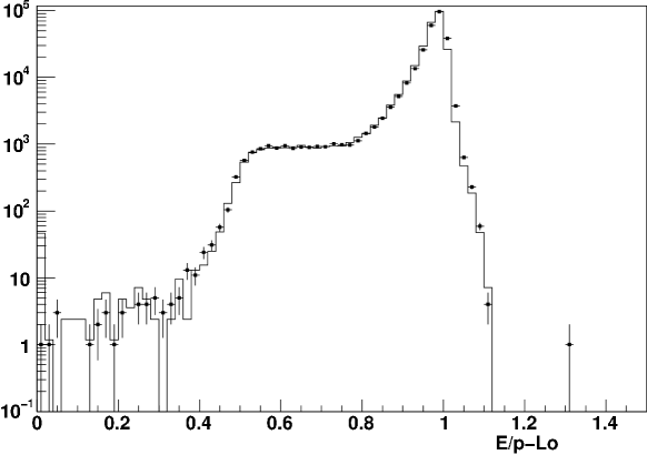
Figure 6.8: Second-largest $E_{\mbox{\scriptsize shower}}/|\vec{p}_{\mbox{\scriptsize track}}|$ divided by $E_{\mbox{\scriptsize beam}}$ in the 10.33 GeV data (points) and Monte Carlo (histogram) with other cuts applied. Data above 0.5 are accepted.

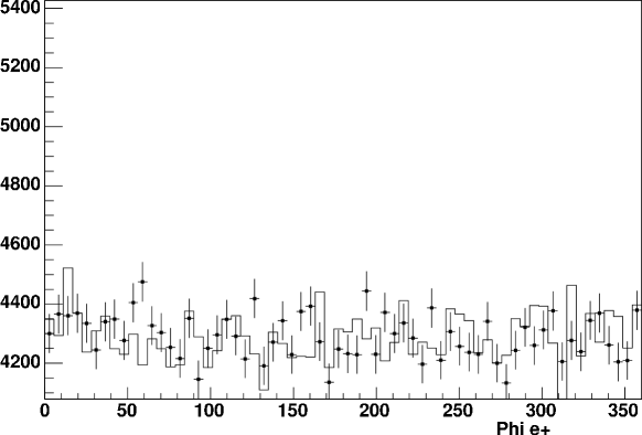
Figure 6.9: Positron $\phi$ (azimuthal angle) distribution in the 10.33 GeV data (points) and Monte Carlo (histogram) with other cuts applied. This variable is not used for cuts.

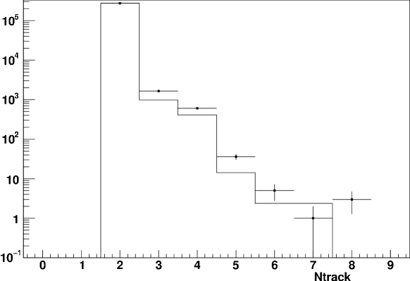
Figure 6.10: Number of charged tracks in the 10.33 GeV data (points) and Monte Carlo (histogram) with other cuts applied. This variable is not used for cuts.

The efficiency-weighted Bhabha cross-sections at 9.43, 10.00, and 10.33 GeV differ by more than $1/s$ because the Monte Carlo finds these Bhabha cuts, particularly the requirement that the energy sum of the two tracks be greater than 90% of $E_{\mbox{\scriptsize CM}}$, to be energy-dependent. We checked this claim by comparing Bhabha counts with $\gamma\gamma$ counts, and by loosening the energy sum cut. Both methods reveal the same 2% per GeV energy dependence from $\Upsilon(1S)$ to $\Upsilon(3S)$.

We additionally determine the efficiency-weighted cross-sections of $e^{+}e^{-}\to\mu^{+}\mu^{-}$ and $e^{+}e^{-}\to\gamma\gamma$ to reduce systematic uncertainties by comparing the luminosity predicted for the same dataset by different processes. We follow the method of [18] to assign 1.6% systematic uncertainties for Bhabha efficiency-weighted cross-section, 1.6% for $\mu^{+}\mu^{-}$, and 1.8% for $\gamma\gamma$. The sources of these uncertainties are tabulated in Table 6.1: $e^{+}e^{-}$ and $\mu^{+}\mu^{-}$ uncertainties are dominated by the degree of resonance interference and the track-finding efficiency, while $\gamma\gamma$ uncertainties are dominated by the photon-finding efficiency and angular resolution.

Table 6.1: Fractional systematic uncertainties in our determinations of the efficiency-weighted cross-sections of $e^{+}e^{-}$, $\mu^{+}\mu^{-}$, and $\gamma\gamma$. All values are percentages.

	$e^{+}e^{-}$	$\mu^{+}\mu^{-}$	$\gamma\gamma$
Finite Monte Carlo sample	0.4	0.5	0.6
Radiative corrections	0.5	0.5	0.5
Resonance interference	1.0	1.0
Trigger efficiency	0.1	0.1	0.7
Track-finding efficiency	1.0	1.0
Photon-finding efficiency			1.0
Dependence on cuts	0.5	0.3	1.0
Cosmic ray backgrounds		0.2
ISR tail backgrounds		0.1
Total	1.6	1.6	1.8

We can compare these as luminosity measurements by dividing the $e^{+}e^{-}$, $\mu^{+}\mu^{-}$, and $\gamma\gamma$ counts from the same sample— all available off-resonance data— by their efficiency-weighted cross-sections. We obtain the integrated luminosities plotted in Figure 6.11, which are in good agreement, considering their systematic uncertainties. The $e^{+}e^{-}$ and $\mu^{+}\mu^{-}$ modes share the same track-finding efficiency, so we draw error bars with this systematic removed in the Figure.

Figure 6.11: The integrated luminosity of all off-resonance data combined, as determined from $e^{+}e^{-}$, $\mu^{+}\mu^{-}$, and $\gamma\gamma$ counts. Outermost errorbars include all systematic uncertainties, and the second errorbars on $e^{+}e^{-}$ and $\mu^{+}\mu^{-}$ have common tracking and resonance interference systematics removed. Innermost errorbars (visible only for $\mu^{+}\mu^{-}$) are statistical-only. The weighted average and RMS of the three measurements are represented by dashed and dotted horizontal lines.

The weighted average luminosity from $e^{+}e^{-}$, $\mu^{+}\mu^{-}$, and $\gamma\gamma$ is only 0.2–0.6% higher than the $e^{+}e^{-}$ luminosity alone (depending on dataset), so we modify our luminosity determination to return the average luminosity from the three processes. The integrated luminosity is

$$0.1114\mbox{ }(E_{\mbox{\scriptsize CM}}/\mbox{9.43~{}GeV})^{2}\mbox{ nb${}^{-1}$\ per observed Bhabha event,}$$ (6.4)

$$0.1266\mbox{ }(E_{\mbox{\scriptsize CM}}/\mbox{10.00~{}GeV})^{2}\mbox{ nb${}^{-1}$\ per observed Bhabha event, and}$$ (6.5)

$$0.1361\mbox{ }(E_{\mbox{\scriptsize CM}}/\mbox{10.33~{}GeV})^{2}\mbox{ nb${}^{-1}$\ per observed Bhabha event}$$ (6.6)

in the three datasets.

Without knowing that $\mu^{+}\mu^{-}$ and $\gamma\gamma$ measurements reproduce the Bhabha result, we would have a 1.6% uncertainty common to all three luminosity scale factors. However, we can incorporate this information by assigning the $e^{+}e^{-}$, $\mu^{+}\mu^{-}$, and $\gamma\gamma$ RMS differences from the average as the common uncertainty. Thus, the luminosity scale factors have an uncertainty of 1.3%. The luminosity scale factor is a factor in $\Gamma_{ee}\Gamma_{\mbox{\scriptsize had}}/\Gamma_{\mbox{\scriptsize tot}}$, so the fractional uncertainty in this scale factor adds to the $\Gamma_{ee}\Gamma_{\mbox{\scriptsize had}}/\Gamma_{\mbox{\scriptsize tot}}$ fractional uncertainty in quadrature.

The systematic uncertainties in the three luminosity scale factors are not independently 1.3%: they will partly cancel in ratios. We can see this by considering the minimum information necessary to determine $\Gamma_{ee}(ns)/\Gamma_{ee}(mS)$. One must know the ratio of Bhabha cut efficiencies near the $\Upsilon(nS)$ and the $\Upsilon(mS)$ and the scaling of Bhabha cut efficiency with $E_{\mbox{\scriptsize CM}}$, but the conversion from the number of Bhabha events to inverse nanobarns will cancel. Thus, the dominant uncertainty in ratios of luminosity scale factors is the ratio of Bhabha cut efficiencies, determined with 0.5% uncertainty by Monte Carlo.

To blind our analysis, we determined the overall luminoisty scale factors last, after all background (Chapter 4), efficiency (Chapter 5), and beam energy studies (Chapter 7) were completed. Until that point, we only knew the ratios of luminosities of our data samples, and therefore only $\Gamma_{ee}(nS)/\Gamma_{ee}(mS)$. We incorporated these scale factors (using $\gamma\gamma$ event counts, rather than Bhabha event counts) just before presenting preliminary $\Gamma_{ee}$ results at the European Physical Society meeting in July, 2005.

6.3 Consistency of Bhabhas with $\gamma\gamma$

Above, we took advantage of the $\gamma\gamma$ luminosity measurement’s very different systematic uncertainties to check and correct the Bhabha scale factors off-resonance, but we have not yet used the fact that $\gamma\gamma$ counts are unaffected by $\Upsilon$ decays. In this Section, we will compare Bhabha and $\gamma\gamma$ rates as a function of $E_{\mbox{\scriptsize CM}}$ through the $\Upsilon$ resonances, to test the $\Upsilon\to e^{+}e^{-}$ correction. We tune the $\gamma\gamma$ luminosity measurement to yield the same results as Bhabhas off-resonance and measure the $\gamma\gamma$ and Bhabha luminosities in $\Upsilon$ data. Both methods should yield the same integrated luminosity, within statistical uncertainties.

In Figure 6.12, we plot ratios of luminosity measurements for off-resonance, scan, and peak data on the $\Upsilon(1S)$, $\Upsilon(2S)$, and $\Upsilon(3S)$, and observe a discrepancy on the $\Upsilon(1S)$ and $\Upsilon(3S)$. The $\gamma\gamma$ luminosity scale factor is tuned to reproduce Bhabha luminosity off-resonance, but not separately for the three off-resonance datasets, so the discrepancy we observe occurs only at the $\Upsilon$ resonances. It is not, therefore, linear with respect to $E_{\mbox{\scriptsize CM}}$, as would be expected if the discrepancy were due to energy-dependent cut efficiencies. (The discrepancy is also 20 times larger than the energy dependence in the Bhabha cuts, and the $\gamma\gamma$ cuts have no energy dependence on this scale.)

Figure 6.12: Ratio of Bhabha luminosity to $\gamma\gamma$ luminosity, with the weighted average continuum ratio set to unity.

The direction of this effect, and the fact that it only influences $\Upsilon$ data, could be explained if we were over-subtracting $\Upsilon\to e^{+}e^{-}$ from our Bhabha count. However, the relative magnitudes of the $\Upsilon(1S)$ and the $\Upsilon(3S)$ discrepancies cannot be accounted for. An over-subtraction error would be proportional to peak hadronic cross-section times ${\mathcal{B}}_{ee}$, which is 0.45 nb for the $\Upsilon(1S)$ and 0.096 nb for the $\Upsilon(3S)$, but the discrepancies appear to be equal. Even considering the uncertainties in these measurements, the over-subtraction hypothesis is ruled out by 8.7 standard deviations.

We do not know whether the discrepancy is due to an error in the Bhabha measurement or in the $\gamma\gamma$ measurement, so we apply half of this discrepancy as a correction and add half the discrepancy and its uncertainty in quadrature to the total uncertainty in luminosity, to cover the ambiguity. This is only a 0.4% uncertainty in the luminosity of each resonance, and therefore a small contributor to the total $\Gamma_{ee}$ uncertainty.

Chapter 7 Beam Energy Measurement

Having presented all the details necessary to properly measure the hadronic $\Upsilon$ cross-section, the vertical axis in our lineshape plot (Figure 2.2), we now consider our measurement of $E_{\mbox{\scriptsize CM}}$, the horizontal axis. In Chapter 3, we discussed the mechanism which determines the beam energy of each run. While this reckoning differs from the true beam energy by 18 MeV near the $\Upsilon$ resonances, we will show in this Chapter that measurements of beam energy differences are robust enough for the precision demands of this analysis.

The masses of the $\Upsilon$ resonances have been measured with 0.3–0.5 MeV precision at Novosibirsk [19], so we can use the $\Upsilon$ lineshapes as calibrating markers in beam energy. If we correct our $E_{\mbox{\scriptsize CM}}$ measurements by a constant shift at the $\Upsilon(1S)$, we almost reproduce the Novosibirsk $\Upsilon(2S)$ and $\Upsilon(3S)$ masses: our average $\Upsilon(2S)$ mass is 0.65 $\pm$ 0.18 MeV too low, and our average $\Upsilon(3S)$ mass is 1.60 $\pm$ 0.30 MeV too low (Figure 7.1). If this error is purely a function of beam energy and is not related to alterations in CESR’s configuration between the $\Upsilon(3S)$, $\Upsilon(1S)$, and $\Upsilon(2S)$ data-taking periods, then our beam energy measurements differ from the true beam energies by a linear transformation, which we determine with a fit to the three apparent $\Upsilon$ masses in Figure 7.1. If this tranformation applies to small changes in beam energy (scan point differences, about 10 MeV) as well as large (300 MeV between resonances), the resonance scans are too narrow, and $\Gamma_{ee}\Gamma_{\mbox{\scriptsize had}}/\Gamma_{\mbox{\scriptsize tot}}$ is too low, by only 0.2%. Because of the uncertainties noted above, we do not apply this as a correction.

Figure 7.1: Difference between the measured mass and the true mass of the $\Upsilon(1S)$, $\Upsilon(2S)$, and $\Upsilon(3S)$, where the $\Upsilon(1S)$ measurement has been shifted to the true mass. Outer errorbars represent the RMS of all scan measurements at each resonance, and inner errorbars are statistical-only. The dashed curve is a linear fit.

Potentially more worrisome are variations in the beam energy with time. The measurement of beam energy differences is sensitive to the placement of the NMR probes in the test magnets, because at the 0.05% level (corresponding to 1 MeV in $E_{\mbox{\scriptsize CM}}$), the magnetic field in the test magnets is a function of position. Every week, these probes are exposed to the possibility of movement as a consequence of CESR machine studies, since these studies may involve reconfiguring the test magnet. To protect our lineshape scans from discrete shifts in beam energy calibration, we divided our data-taking into short, independent 10-hour scans, plus 38 hours of subsequent peak running, separated by about a week. The test magnets were not disturbed during these dedicated scans or during the peak data-taking associated with each scan. Changes in the apparent $\Upsilon$ mass from one week to the next alert us to shifts in the beam energy measurement between scans, which we observe as a slow drift on the order of 0.5 MeV per month (Figure 7.2). To be insensitive to these drifts, we include the apparent $\Upsilon$ mass of each 10+38-hour scan as an independent parameter in the lineshape fit. Values of $E_{\mbox{\scriptsize CM}}$ in the lineshape fit are only relative to the apparent $\Upsilon$ mass from the week the data were taken.

Figure 7.2: Difference between the measured mass and the true mass of the $\Upsilon(1S)$, $\Upsilon(2S)$, and the $\Upsilon(3S)$ (top to bottom), for each individual scan. Dashed horizontal lines represent the weighted averages.

We are only sensitive to random changes in the beam energy calibration (true $E_{\mbox{\scriptsize beam}}$ $-$ measured $E_{\mbox{\scriptsize beam}}$), or jitter, on a 10-hour timescale. We have already ensured our insensitivity to week-by-week fluctuations. If the beam energy fluctuates on very short timescales, much less than an hour (the length of a run), then the jitter only contributes to beam energy spread. (In this sense, the beam energy fluctuates by about 4 MeV with every collision!) We reduce our sensitivity to monotonic 10-hour calibration drifts by alternating scan points above and below the $\Upsilon$ peak, so that a drift would not systematically widen or narrow the lineshape.

To check for changes in the beam energy calibration on the 10-hour timescale, we measure the cross-section at a high-derivative point on the lineshape twice, usually at the beginning and end of a scan. Since the derivative is high, significantly different cross-section results at the same reported beam energy would be an indication that the actual beam energy has shifted between the two measurements. Any cross-section difference ($\sigma_{1}-\sigma_{2}$) can be converted into a true beam energy difference ($E_{1}-E_{2}$) at a given lineshape derivative ($d\sigma/dE$) by

$$\left.E_{1}-E_{2}=\frac{\sigma_{1}-\sigma_{2}}{d\sigma/dE}\right._{\mbox{.}}$$ (7.1)

To find possible shifts in calibration, we subtract the true beam energy difference from the reported difference, and propagate uncertainties from the cross-section measurement. We call this a shift ($s_{i}\pm\delta_{s_{i}}$). The shifts (plotted in Figure 7.3) are not quite consistent with zero, as the total $\chi^{2}=\sum_{i}(s_{i}/\delta_{s_{i}})^{2}$ is 31.2 for 29 degrees of freedom (a 0.64% confidence level). This broadening of the $\{s_{i}\}$ distribution can be accomodated by a uniformly-random jitter $j$. To quantify $j$, we construct a log-likelihood function of the $\{s_{i}\}$ data, assuming them to be Gaussian-distributed with statistical and jitter components to the width.

$$L(j)=\sum_{i=1}^{29}\ln\left(\frac{1}{\sqrt{2\pi({\delta_{s_{i}}}^{2}+j^{2})}}\exp\left(\frac{-{s_{i}}^{2}}{2({\delta_{s_{i}}}^{2}+j^{2})}\right)\right)$$ (7.2)

Only jitters larger than 0.05 MeV are inconsistent with the data at the 68% confidence level (the value of $j$ necessary to lower the log-likelihood by 1/2; see Figure 7.4). Alternatively, we could have constructed an $S$-factor in analogy with the Particle Data Group’s method of calculating uncertainty from a set of mutually-inconsistent experiments:

$$\left.S(j)=\sum_{i=1}^{29}\frac{{s_{i}}^{2}}{{\delta_{s_{i}}}^{2}+j^{2}}\right._{\mbox{.}}$$ (7.3)

In this formulation, the maximally-allowed jitter is the value which reduces $S(j)$ to unity, which is $j=0.07$ MeV. Both methods yield roughly the same value, so we can be confident that the beam energy calibration jitter is approximately 0.07 MeV, which is 7 parts per million.

Figure 7.3: Beam energy shifts ($s_{i}$) determined by pairs of repeated cross-section measurements, plotted with respect to the time between the first and the second measurement. The weighted mean of $\{s_{i}\}$ is 0.02 $\pm$ 0.03 MeV, so the apparent vertical asymmetry of this distribution is an illusion.

Figure 7.4: Log-likelihood ($L(j)$) as a function of jitter ($j$) attains a maximum near $j=0$ and is reduced by 1/2 at $j=0.05$ MeV.

To learn what fluctuations of this size imply for uncertainty in $\Gamma_{ee}\Gamma_{\mbox{\scriptsize had}}/\Gamma_{\mbox{\scriptsize tot}}$, we simulated the lineshape fits with random perturbations in the measured beam energy. The nominal $E_{\mbox{\scriptsize CM}}$ and luminosity of each simulated cross-section measurement were copied from the real data sample, but the cross-sections themselves were derived from an ideal curve with statistical errors. Without perturbing the simulated beam energy measurements, the fits return our input $\Gamma_{ee}\Gamma_{\mbox{\scriptsize had}}/\Gamma_{\mbox{\scriptsize tot}}$ with perfectly-distributed fit $\chi^{2}$ values. When $E_{\mbox{\scriptsize CM}}$ is randomly perturbed with a standard deviation of 0.07 MeV, the value of $\Gamma_{ee}\Gamma_{\mbox{\scriptsize had}}/\Gamma_{\mbox{\scriptsize tot}}$ fluctuates up and down by 0.2% of itself, and the $\chi^{2}$ increases by only 5–30 units. We therefore assign a 0.2% systematic uncertainty in $\Gamma_{ee}\Gamma_{\mbox{\scriptsize had}}/\Gamma_{\mbox{\scriptsize tot}}$ and $\Gamma_{ee}$ due to beam energy measurement errors.

Chapter 8 Lineshape Fitting

We have reached the core of the analysis, the fits of the $\Upsilon$ lineshapes. All previous studies either deliver data to these fits or define the curve that the data are fit to. In this Chapter, we will review the fit function and all of its parameters, present the fit results, and discuss hadron-level interference as a fitting issue.

8.1 The Fit Function

8.1.1 Hadronic Peak

The central feature of the fit function is a Breit-Wigner curve representing the hadronic cross-section (Equation 2.3), convoluted with beam energy spread and initial-state radiation (ISR). The beam energy spread is modeled by a Gaussian with unit area, and the ISR distribution is calculated to fourth order in perturbative QED by Kuraev and Fadin [20] (Equation (28)).

Most of the floating parameters of the fit modify this contribution. The area of the Breit-Wigner is the most important floating parameter, as this is how we determine $\Gamma_{ee}\Gamma_{\mbox{\scriptsize had}}/\Gamma_{\mbox{\scriptsize tot}}$ and $\Gamma_{ee}$ (Equation 2.2). To let each 48-hour scan’s $\Upsilon$ mass float independently (Section 7.1 on page 7.1), we fix the mass in the fit function and allow the $E_{\mbox{\scriptsize CM}}$ measurements in the data to be shifted scan-by-scan. This way, when we plot the lineshape fits, a single curve represents the fit to all data. In Chapter 3, we discussed the variability of beam energy spread (Section 3.1 on page 3.1). To allow scans to have different beam energy spreads (Gaussian widths), we use different fit curves. We do not transform the data in analogy with the mass shifts because the ISR tail spoils the linearity of the transformation.

The full width $\Gamma$ is a parameter in the Breit-Wigner distribution, but we do not allow this parameter to float. Our fitted $\Gamma_{ee}\Gamma_{\mbox{\scriptsize had}}/\Gamma_{\mbox{\scriptsize tot}}$ is sensitive to $\Gamma$ only at the 0.03% level, so we fix each $\Gamma$ to its previously measured value [21].

The hadronic $\Upsilon$ efficiency is another multiplicative constant in our fit function. We multiply our fit function by efficiency rather than dividing our data by efficiency because our data includes several different components, each with a different efficiency.

We add interference with the continuum (Section 2.3 on page 2.3) to the Breit-Wigner before convolution. That is, the signal lineshape is

$$\tilde{\sigma}_{{\mbox{\scriptsize res}}+{\mbox{\scriptsize int}}}(E_{\mbox{\scriptsize CM}})=\bigg{(}\sigma_{\mbox{\scriptsize res}}(E^{\prime})+\tilde{\sigma}_{\mbox{\scriptsize int}}(E^{\prime})\bigg{)}\otimes G\otimes ISR$$ (8.1)

where $\sigma_{\mbox{\scriptsize res}}$ and $\tilde{\sigma}_{\mbox{\scriptsize int}}$ are defined in Equation 2.5 and $\otimes$ represents convolution with the beam energy spread Gaussian ($G$) and the ISR distribution ($ISR$). This $\tilde{\sigma}_{{\mbox{\scriptsize res}}+{\mbox{\scriptsize int}}}$ does not represent a physical cross-section until we add the continuum piece. (It is negative for some values of $E_{\mbox{\scriptsize CM}}$.) The interference between resonant and continuum $q\bar{q}$ decays is characterized by two constants, $\phi_{0}$ and $\alpha_{\mbox{\scriptsize int}}$ (Equation 2.8), both of which are known and do not need to float in the fit.

8.1.2 Tau-Pair Peak

The $\tau^{+}\tau^{-}$ background term has the same form as the hadronic signal term: it is the sum of a Breit-Wigner and $\tilde{\sigma}_{\mbox{\scriptsize int}}^{\tau^{+}\tau^{-}}$, convoluted by the same beam energy spread and ISR distribution. This term introduces no new floating parameters: the Breit-Wigner area for $\tau^{+}\tau^{-}$ is the Breit-Wigner area for hadronic $\Upsilon$, multiplied by a ratio of branching fractions and efficiencies

$$\frac{\mbox{area}_{\tau^{+}\tau^{-}}}{\mbox{area}_{\mbox{\scriptsize had}}}=\left.\frac{{\mathcal{B}}_{\tau^{+}\tau^{-}}}{{\mathcal{B}}_{\mbox{\scriptsize had}}}\times\frac{\epsilon_{\tau^{+}\tau^{-}}}{\epsilon_{\mbox{\scriptsize had}}}\right._{\mbox{.}}$$ (8.2)

The value of ${\mathcal{B}}_{\tau\tau}$ we use in the fit function is from [22]. We use this value to determine $\Gamma_{ee}\Gamma_{\mbox{\scriptsize had}}/\Gamma_{\mbox{\scriptsize tot}}$, but when we determine $\Gamma_{ee}$, we perform a separate fit with ${\mathcal{B}}_{\tau\tau}$ = ${\mathcal{B}}_{\mu\mu}$ and ${\mathcal{B}}_{\mu\mu}$ from [12]. This allows us to subtract $\tau^{+}\tau^{-}$ backgrounds with the same branching fraction that we use to multiply it back in, when we convert $\Gamma_{ee}\Gamma_{\mbox{\scriptsize had}}/\Gamma_{\mbox{\scriptsize tot}}$ to $\Gamma_{ee}$ (Equation 2.10).

The magnitude of interference, $\alpha_{\mbox{\scriptsize int}}^{\tau^{+}\tau^{-}}$, is also different for the $\tau^{+}\tau^{-}$ peak, because $\sigma(e^{+}e^{-}\to\tau^{+}\tau^{-})$ and $\Gamma(\Upsilon\to\tau^{+}\tau^{-})$ are not equal to $\sigma(e^{+}e^{-}\to q\bar{q})$ and $\Gamma(\Upsilon\to q\bar{q})$, respectively.

8.1.3 Background Terms

We add a single $1/s$ term to the fit function to represent continuum $q\bar{q}$, radiative Bhabhas, $\tau^{+}\tau^{-}$, and any residual Bhabha or $\mu^{+}\mu^{-}$ backgrounds. The magnitude of this term floats in the fit, though it is primarily influenced by our large off-resonance data point.

The resonance interferes with only part of the contniuum, so the magnitude of resonance interference is not tied to the fitted value of the $1/s$ term. The $q\bar{q}$ and $\tau^{+}\tau^{-}$ cross-sections that enter into $\alpha_{\mbox{\scriptsize int}}$ and $\alpha_{\mbox{\scriptsize int}}^{\tau^{+}\tau^{-}}$ are either derived from other experiments ([9] for $\alpha_{\mbox{\scriptsize int}}$) or are calculated from QED (for $\alpha_{\mbox{\scriptsize int}}^{\tau^{+}\tau^{-}}$).

This dissociation of the continuum cross-section from the interference term is artificial, since interference is only meaningful in the presence of both resonance and continuum amplitudes. It would be more natural, for instance, to include the continuum cross-section in the beam energy spread and ISR convolutions with the resonance and interference terms, since the natural lineshape includes all three terms before it is smeared by the physical beams. However, the continuum cross-section doesn’t depend on $E_{\mbox{\scriptsize CM}}$ sharply enough for this to matter.

For $\Upsilon(2S)$ and $\Upsilon(3S)$ fits, we add the fitted lineshape(s) from $\Upsilon(1S)$ and $\Upsilon(2S)$ as backgrounds, because the ISR tails from these resonances introduce 0.4–0.6% corrections. These background components do not float in the fit. (We fit the three resonances separately.)

The $\log s$ correction motivated by two-photon fusion backgrounds is tied to the overall continuum normalization through $f$ = 0.080 $\pm$ 0.005, the fraction of $\log s$ component to $1/s$ at 9 GeV, determined by a fit from Section 4.14 on page 4.14. The total continuum cross-section is therefore

$$\sigma_{\mbox{\scriptsize cont}}(E_{\mbox{\scriptsize CM}})=\sigma_{\mbox{\scriptsize cont}}^{0}\left((1-f)\frac{(\mbox{9~{}GeV})^{2}}{{E_{\mbox{\scriptsize CM}}}^{2}}+f\log\frac{{E_{\mbox{\scriptsize CM}}}^{2}}{(\mbox{9~{}GeV})^{2}}\right)$$ (8.3)

where $\sigma_{\mbox{\scriptsize cont}}^{0}$ is the floating parameter.

We allow $\sigma_{\mbox{\scriptsize cont}}^{0}$ to float independently in the $\Upsilon(1S)$, $\Upsilon(2S)$, and $\Upsilon(3S)$ fits. Since it represents the cross-section at a fixed $E_{\mbox{\scriptsize CM}}$, the three fits ought to return the same value. Instead, the $\Upsilon(1S)$, $\Upsilon(2S)$, and $\Upsilon(3S)$ fits yield 9.355 $\pm$ 0.010 nb, 9.318 $\pm$ 0.007 nb, and 9.315 $\pm$ 0.011 nb, respectively. The $\Upsilon(2S)$ and $\Upsilon(3S)$ values are consistent with each other, but the $\Upsilon(1S)$ fit has a $\sigma_{\mbox{\scriptsize cont}}^{0}$ which is 3.0 standard deviations higher than $\Upsilon(2S)$. However, this difference in $\sigma_{\mbox{\scriptsize cont}}^{0}$ values is only 0.04% of $\sigma_{\mbox{\scriptsize cont}}^{0}$ itself. It is possible that our ISR tail corrections are too large, an error which is absorbed into $\sigma_{\mbox{\scriptsize cont}}^{0}$, rather than biasing the fit for $\Gamma_{ee}\Gamma_{\mbox{\scriptsize had}}/\Gamma_{\mbox{\scriptsize tot}}$.

8.1.4 Summary of all Floating Parameters

The $\Upsilon(1S)$ fit has a total of sixteen parameters: $\Gamma_{ee}\Gamma_{\mbox{\scriptsize had}}/\Gamma_{\mbox{\scriptsize tot}}$, $M_{1},\ldots M_{11}$ for its eleven 48-hour scans, $\Delta E_{1}$, $\Delta E_{2}$, and $\Delta E_{3}$ for its three groups of scans with potentially different beam energy spreads (see Table 3.1), and $\sigma_{\mbox{\scriptsize cont}}^{0}$ for the continuum background normalization at 9 GeV.

The $\Upsilon(2S)$ fit has a total of nine floating parameters: $\Gamma_{ee}\Gamma_{\mbox{\scriptsize had}}/\Gamma_{\mbox{\scriptsize tot}}$, $M_{1},\ldots,M_{6}$ for its six 48-hour scans, a single beam energy spread $\Delta E$ (the CESR orbits were stable), and $\sigma_{\mbox{\scriptsize cont}}^{0}$.

The $\Upsilon(3S)$ fit has a total of sixteen floating parameters: $\Gamma_{ee}\Gamma_{\mbox{\scriptsize had}}/\Gamma_{\mbox{\scriptsize tot}}$, $M_{1},\ldots,M_{7}$ for its seven 48-hour scans, $\Delta E_{1},\ldots,\Delta E_{7}$, a beam energy spread for each scan, and $\sigma_{\mbox{\scriptsize cont}}^{0}$.

8.2 Systematic Uncertainties from Constants in the Fit

Each constant in the fit function may introduce systematic error, but in every case, this error is negligible. Kuraev and Fadin estimate that their ISR calculation has a 0.1% uncertainty; varying the tail normalization by this amount changes our $\Gamma_{ee}\Gamma_{\mbox{\scriptsize had}}/\Gamma_{\mbox{\scriptsize tot}}$ result by 0.05%. As previously mentioned, the uncertainty in $\Gamma$ affects our result by less than 0.03%. Uncertainty in the $q\bar{q}$ interference magnitude (from $R$) yields a 0.02% uncertainty, and the $\tau^{+}\tau^{-}$ interference magnitude (from ${\mathcal{B}}_{\tau\tau}$) yields 0.08%. Uncertainty in the two-photon fraction $f$ yields 0.002%. The sum of all of these uncertainties in quadrature is 0.10%.

We do not propagate the uncertainty in the $\tau^{+}\tau^{-}$ efficiency (first mentioned in Section 8.2 on page 8.2) because it is multiplied by ${\mathcal{B}}_{\tau\tau}$ or ${\mathcal{B}}_{\mu\mu}$ (in the $\Gamma_{ee}\Gamma_{\mbox{\scriptsize had}}/\Gamma_{\mbox{\scriptsize tot}}$ and $\Gamma_{ee}$ fits, respectively). The fractional uncertainty in the Monte Carlo modeling of $\tau^{+}\tau^{-}$ efficiency is not significantly greater than 2%, the smallest ${\mathcal{B}}_{\tau\tau}$ or ${\mathcal{B}}_{\mu\mu}$ fractional uncertainty.

The hadronic efficiency also enters the fit function as a constant, but we will treat this as a major systematic uncertainty in the next Chapter.

8.3 Fit Results

We used a C++ version (1.5.2) of MINUIT from the SEAL package [23] to perform a $\chi^{2}$ fit of our cross-section data to our fit function. The resulting best-fit values for the Breit-Wigner area used in determining $\Gamma_{ee}$ are presented in Table 8.1. The best-fit functions are plotted in Figure 8.1, and Figures 8.2–8.4, overlaying data. At the top of Figure 8.1 and in Figures 8.5, 8.6, and 8.7 are pull distributions. Pull is the ratio of residual to uncertainty, expressing the significance of deviations from the best-fit line. All data points are visible in these plots; no point has a pull greater than 3.5. Best-fit $\Upsilon$ masses and beam energy spreads are plotted in Figures 7.2 and 3.2, respectively.

Table 8.1: Best-fit Breit-Wigner area and $\chi^{2}$ significance.

	$\int\sigma(e^{+}e^{-}\to\Upsilon\to\mbox{hadronic})\,dE_{\mbox{\scriptsize CM}}$	reduced $\chi^{2}$	confidence level
$\Upsilon(1S)$	324.12 $\pm$ 0.92 MeV nb	$\displaystyle\frac{240.4}{203-16}$ = 1.29	0.51%
$\Upsilon(2S)$	133.65 $\pm$ 0.94 MeV nb	$\displaystyle\frac{107.2}{75-9}$ = 1.62	0.10%
$\Upsilon(3S)$	89.25 $\pm$ 0.88 MeV nb	$\displaystyle\frac{154.5}{175-16}$ = 0.97	58.6%

Figure 8.1: Best-fit lineshapes (solid) to the $\Upsilon(1S)$, $\Upsilon(2S)$, and $\Upsilon(3S)$ data (points), from which $\Gamma_{ee}\Gamma_{\mbox{\scriptsize had}}/\Gamma_{\mbox{\scriptsize tot}}$ is determined. Dashed curves are total background estimates, and the pull distributions above each plot indicate the statistical significance of all deviations from the best-fit line. Insets for each resonance present a tail measurement 100 MeV, 60 MeV, and 45 MeV above the $\Upsilon(1S)$, $\Upsilon(2S)$, and $\Upsilon(3S)$ masses. (Fit functions with multiple beam energy spreads are represented by their average beam energy spread.)

Figure 8.2: Best-fit $\Upsilon(1S)$ lineshape, overlaid upon data from individual scans.

Figure 8.3: Best-fit $\Upsilon(2S)$ lineshape, overlaid upon data from individual scans.

Figure 8.4: Best-fit $\Upsilon(3S)$ lineshape, overlaid upon data from individual scans.

Figure 8.5: The pull distribution of $\Upsilon(1S)$ lineshape fits (a) as a function of $E_{\mbox{\scriptsize CM}}$, (b) as a function of date, and (c), as a histogram, fitted to a Gaussian curve, which is almost two standard deviations wider than unity.

Figure 8.6: The pull distribution of $\Upsilon(2S)$ lineshape fits (a) as a function of $E_{\mbox{\scriptsize CM}}$, (b) as a function of date, and (c), as a histogram, fitted to a Gaussian curve, which is almost two standard deviations wider than unity.

Figure 8.7: The pull distribution of $\Upsilon(3S)$ lineshape fits (a) as a function of $E_{\mbox{\scriptsize CM}}$, (b) as a function of date, and (c), as a histogram, fitted to a Gaussian curve, which is statistically consistent with unity.

This fit function describes our data well: no trends are evident in pull versus energy, but the $\Upsilon(1S)$ and especially the $\Upsilon(2S)$ pull distributions are wider than would be expected from statistical fluctuations. We can also see this by noting that the $\chi^{2}$ per degree of freedom ($N_{\mbox{\scriptsize dof}}$) is improbably high (Table 8.1). In the $\Upsilon(2S)$ data, the high-energy tail is the largest deviation, contributing 9.1 units to the total $\chi^{2}$, but this is only a fifth of the excess. (Dropping this point changes the $\Upsilon(2S)$ $\Gamma_{ee}\Gamma_{\mbox{\scriptsize had}}/\Gamma_{\mbox{\scriptsize tot}}$ by 0.4%.) The simulations of fits with jittering beam energy, described at the end of Section 7.4 on page 7.4 demonstrate that uncertain beam energy measurements can increase the fit $\chi^{2}$ by 5–30 units. If the $\Upsilon(1S)$ and $\Upsilon(2S)$ $\chi^{2}$ values have both been artificially raised 30 units by jittering beam energy measurements, their natural confidence levels would be 10–15%, but there is no conclusive evidence that beam energy jitter is the cause, and assuming an increase of 30 units of $\chi^{2}$ is the most extreme hypothesis.

The larger-than-expected deviations are symmetric around the best-fit line for all $E_{\mbox{\scriptsize CM}}$ and dates, and they do not favor a particular $E_{\mbox{\scriptsize CM}}$ or date (Figures 8.5–8.7), so we treat them as though we had underestimated our statistical uncertainty ($\sigma_{\mbox{\scriptsize stat}}$). We add $\sigma_{\mbox{\scriptsize stat}}\sqrt{\chi^{2}/N_{\mbox{\scriptsize dof}}-1}$ to our systematic uncertainty in quadrature, which has the same effect on the total uncertainty as if we had multiplied $\sigma_{\mbox{\scriptsize stat}}$ by $\sqrt{\chi^{2}/N_{\mbox{\scriptsize dof}}}$.

Note that our fit does not suggest that the beam energy spread distribution is distorted from a pure Gaussian. If this were the case, we would observe trends in pull versus $E_{\mbox{\scriptsize CM}}$. Therefore, our assumption of a Gaussian beam energy spread is valid for our level of precision (statistical plus the above-mentioned systematic uncertainty, which is roughly $\pm 0.1$ nb).

8.4 Hadron-Level Interference

In our fit function, we assumed that continuum and $\Upsilon$ decays only interfere at the parton level, and not at the hadron level. That is, we assume that $e^{+}e^{-}\to q\bar{q}$ can interfere with $e^{+}e^{-}\to\Upsilon\to q\bar{q}$ but not $e^{+}e^{-}\to\Upsilon\to ggg$, even though both $q\bar{q}$ and $ggg$ hadronize into some of the same final states.

This $q\bar{q}$-only scheme optimizes the $\Upsilon(1S)$ fit, assuming no phase difference between resonance and continuum at $E_{\mbox{\scriptsize CM}}\ll M_{\Upsilon}$ ($\phi_{0}=0$). We determined this by repeatedly fitting our lineshape, assuming different interference magnitudes $\alpha_{\mbox{\scriptsize int}}$ (defined in Equation 2.8). We plot the $\chi^{2}$ of these fits in Figure 8.8. The interference magnitude $\alpha_{\mbox{\scriptsize int}}$ is proportional to the square root of the branching fraction of $\Upsilon$ to the interfering final state, which is $\sqrt{{\mathcal{B}}_{\mbox{\scriptsize int}}}=\sqrt{8.9\%}$ for $q\bar{q}$. Our fit is optimized by $\alpha_{\mbox{\scriptsize int}}=0.016\pm 0.004$, or ${\mathcal{B}}_{\mbox{\scriptsize int}}=7.8\pm 4.2$. The $\chi^{2}$ of the $\Upsilon(1S)$ fit with no interference is 15 units larger than our $q\bar{q}$-only scheme, which corresponds to 3.7 standard deviations.

Figure 8.8: A fit of the $\Upsilon(1S)$ for the magnitude of hadronic interference ($\alpha_{\mbox{\scriptsize int}}$), assuming $\phi_{0}=0$. The points are $\Upsilon(1S)$ fits with trial $\alpha_{\mbox{\scriptsize int}}$ values, the vertical axis is the $\chi^{2}$ of these fits, and the solid line is a parabola drawn through the points. Dashed and dotted lines indicate the minimum and 68% confidence level bands, and the circled point represents the $q\bar{q}$-only fit we used in this anaysis.

However, if $e^{+}e^{-}\to\Upsilon\to ggg\to$ hadrons and $e^{+}e^{-}\to q\bar{q}\to$ hadrons significantly interfere, the phase difference $\phi_{0}$ need not be zero. Strong and Electromagnetic $\Upsilon$ decays to hadrons can differ in phase, an effect which has been observed in exclusive decays of charmonium [24] [25]. This Strong minus Electromagnetic ($ggg-q\bar{q}$) phase difference is constant with respect to $E_{\mbox{\scriptsize CM}}$, which gives the resonance minus continuum phase difference a constant offset as it evolves through the resonance peak. In this case, $\phi_{0}$ need not be zero, and our fit is less well constrained.

The question of whether $ggg$ and $q\bar{q}$ interfere inclusively (in the sum over all hadronic final states) is fundamental and interesting in its own right, concerning the quantum mechanics of the hadronization process. Unfortunately, our data cannot answer this question for all phases, because if $\phi_{0}\approx\pm\pi/2$, the interference term $\tilde{\sigma}_{\mbox{\scriptsize int}}$ has the same $E_{\mbox{\scriptsize CM}}$ dependence as the resonance Breit-Wigner (Equation 2.8). It has been argued [26] that inclusive $ggg$/$q\bar{q}$ interference is a small effect because every exclusive final state may have a different $ggg$/$q\bar{q}$ phase. The sum of interference cross-terms includes cancellations and therefore grows more slowly with the number of exclusive final states than the direct cross-section terms.

Though improbable, it is possible that exclusive final states add coherently, such that the inclusive $ggg$ and $q\bar{q}$ cross-sections significantly interfere with $ggg-q\bar{q}$ phase angle $\phi_{ggg}$. The magnitude of this interference cannot be maximal, since some $ggg$ final states are distinguishable from $q\bar{q}$ decays. We define $f_{ggg}$ as the fraction of the $ggg$ amplitude which interferes with $q\bar{q}$. If $\phi_{ggg}=0$, our previous study applies (Figure 8.8) and $f_{ggg}<0.12$ at 95% confidence level. We can also put limits on $f_{ggg}$ which are independent of $\phi_{ggg}$ by considering the fact that $ggg$ and $q\bar{q}$ have different quantum numbers. One-third of the $q\bar{q}$ amplitude is $c\bar{c}$, but $\Upsilon(1S)\to ggg\to c\bar{c}$ is negligible [27]. Moreover, Strong decays preserve the $\Upsilon$ meson’s isospin of $I=0$, while Electromagnetic decays through a virtual photon have $I=0$ or $1$. At most half of the $u\bar{u}$ and $d\bar{d}$ has $I_{z}=0$, and therefore overlap with $ggg$. Adding these fractions yields

$$\begin{array}[]{c}c\bar{c}\\ \frac{2}{3}\end{array}\mbox{}\begin{array}[]{c}\\ \times\end{array}\mbox{}\begin{array}[]{c}\\ 0\end{array}\begin{array}[]{c}\\ +\end{array}\begin{array}[]{c}s\bar{s}\\ \frac{1}{3}\end{array}\mbox{}\begin{array}[]{c}\\ \times\end{array}\mbox{}\begin{array}[]{c}\\ 1\end{array}\begin{array}[]{c}\\ +\end{array}\left(\begin{array}[]{c}d\bar{d}\\ \frac{1}{3}\end{array}\begin{array}[]{c}\\ +\end{array}\begin{array}[]{c}u\bar{u}\\ \frac{2}{3}\end{array}\right)\mbox{}\begin{array}[]{c}\\ \times\end{array}\mbox{}\begin{array}[]{c}\\ 0.5\end{array}\begin{array}[]{c}\\ =\end{array}\begin{array}[]{c}\\ 42\%\end{array}$$ (8.4)

or $f_{ggg}\lesssim 0.4$.

Our $\Upsilon(1S)$ fits constrain $f_{ggg}$ as a function of $\phi_{ggg}$. Assuming $\phi_{ggg}$ values between $0$ and $2\pi$, we fit for the maximum $f_{ggg}$ consistent with the data at the 68% confidence level (the value which raises the fit $\chi^{2}$ by one unit), and plot this allowed region in Figure 8.9. For most of the $\phi_{ggg}$ range, our fit is more restrictive than the constraint we derived from flavor and isospin considerations, though within 0.2 rad of $\pm\pi/2$, our fit yields no information. Outside of this range, the minimum $\chi^{2}$ is attained within $0<f_{ggg}<0.1$.

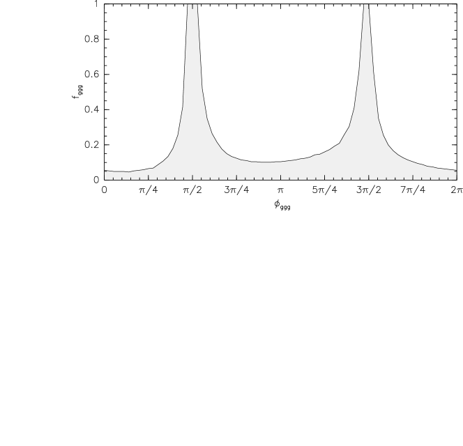
Figure 8.9: The fraction of $ggg$ amplitude allowed to interfere with continuum $q\bar{q}$ ($f_{ggg}$), according to the $\Upsilon(1S)$ fit at 68% confidence level. We have no sensitivity to this parameter if the $ggg-q\bar{q}$ phase difference in $\Upsilon$ decays ($\phi_{ggg}$) is near $\pm\pi/2$.

Hadron-level interference also affects our $\Gamma_{ee}\Gamma_{\mbox{\scriptsize had}}/\Gamma_{\mbox{\scriptsize tot}}$ result, especially for $\phi_{ggg}$ near $\pm\pi/2$. From the same fits, we derive the following relationship between the correction that must be applied to $\Gamma_{ee}\Gamma_{\mbox{\scriptsize had}}/\Gamma_{\mbox{\scriptsize tot}}$ and $f_{ggg}$ and $\phi_{ggg}$.

$$\Delta(\Gamma_{ee}\Gamma_{\mbox{\scriptsize had}}/\Gamma_{\mbox{\scriptsize tot}})=-5.42\%\bigg{(}f_{ggg}\,\sin(\phi_{ggg}+0.3)\bigg{)}+0.14\%\bigg{(}f_{ggg}+0.92\,{f_{ggg}}^{2}\bigg{)}$$ (8.5)

Applying the limits on $f_{ggg}$ shown in Figure 8.9 to Equation 8.5, we obtain the 68% confidence level upper limits on $\Upsilon(1S)$ $\Gamma_{ee}\Gamma_{\mbox{\scriptsize had}}/\Gamma_{\mbox{\scriptsize tot}}$ corrections shown in Figure 8.10. Corrections for the $\Upsilon(2S)$ are 70% as large as this and corrections for the $\Upsilon(3S)$ are 65% as large.

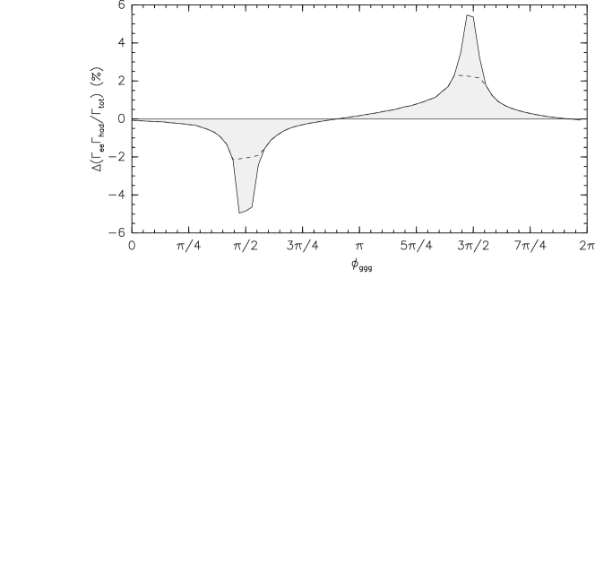
Figure 8.10: The possible correction to $\Gamma_{ee}\Gamma_{\mbox{\scriptsize had}}/\Gamma_{\mbox{\scriptsize tot}}$ implied by our ignorance of $f_{ggg}$ at 68% confidence level (gray) as a function of $\phi_{ggg}$. The dashed lines represent upper limits including isospin and flavor arguments.

Complete a priori ignorance of inclusive $ggg$/$q\bar{q}$ interference would imply a 2.0% uncertainty in $\Gamma_{ee}\Gamma_{\mbox{\scriptsize had}}/\Gamma_{\mbox{\scriptsize tot}}$ and $\Gamma_{ee}$ for the $\Upsilon(1S)$, a 1.4% uncertainty for the $\Upsilon(2S)$, and a 1.3% uncertainty for the $\Upsilon(3S)$. However, the possibility that $f_{ggg}$ is as large as 0.4 is not widely believed to be likely, nor is it clear that $\phi_{ggg}\approx\pm\pi/2$

Chapter 9 Results and Conclusions

In this Chapter, we present final results for $\Gamma_{ee}\Gamma_{\mbox{\scriptsize had}}/\Gamma_{\mbox{\scriptsize tot}}$, for $\Gamma_{ee}$, for $\Gamma_{ee}(nS)/\Gamma_{ee}(mS)$, for $\Gamma$, and for $|\psi(0,0,0)|^{2}$, all of which are derived from $\Gamma_{ee}\Gamma_{\mbox{\scriptsize had}}/\Gamma_{\mbox{\scriptsize tot}}$. But first, we review the systematic uncertainties in $\Gamma_{ee}\Gamma_{\mbox{\scriptsize had}}/\Gamma_{\mbox{\scriptsize tot}}$.

The hadronic $\Upsilon$ efficiency and integrated luminosity scale factor together determine the multiplicative scale for cross-section, so fractional uncertainties in these two factors add in quadrature to the fractional uncertainty in $\Gamma_{ee}\Gamma_{\mbox{\scriptsize had}}/\Gamma_{\mbox{\scriptsize tot}}$. Uncertainties in backgrounds contribute negligibly to systematic uncertainty (their largest effect is statistical). At the end of Chapter 7, we determined the effect of beam energy uncertainty on the lineshape fits through simulations, and in Section 8.2, we determined the uncertainty due to the parameterization of our fit function. Our data have two unexplained features: Bhabhas and $\gamma\gamma$ events do not predict the same luminosity as a function of $E_{\mbox{\scriptsize CM}}$, and the fit $\chi^{2}$ is significantly higher than the number of degrees of freedom for the $\Upsilon(1S)$ and $\Upsilon(2S)$. We have quantified both of these as systematic uncertainties. All uncertainties in $\Gamma_{ee}\Gamma_{\mbox{\scriptsize had}}/\Gamma_{\mbox{\scriptsize tot}}$ and $\Gamma_{ee}$ are listed in Table 9.1, including uncertainty from the correction for leptonic modes (Equation 2.10), which applies to $\Gamma_{ee}$ and not $\Gamma_{ee}\Gamma_{\mbox{\scriptsize had}}/\Gamma_{\mbox{\scriptsize tot}}$.

Table 9.1: All uncertainties in $\Gamma_{ee}\Gamma_{\mbox{\scriptsize had}}/\Gamma_{\mbox{\scriptsize tot}}$ and $\Gamma_{ee}$. The “correction for leptonic modes” applies to $\Gamma_{ee}$ only, and “common hadronic efficiency” and “overall luminosity scale” are common to all three resonances.

Contribution to $\Gamma_{ee}$	$\Upsilon(1S)$	$\Upsilon(2S)$	$\Upsilon(3S)$
Common hadronic efficiency (Section 5.2)	${}^{+0.4}_{-0.6}$%	${}^{+0.4}_{-0.6}$%	${}^{+0.4}_{-0.6}$%
$\Upsilon(2S)$, $\Upsilon(3S)$ efficiency corrections (Section 5.3)	0	0.15%	0.13%
Overall luminosity scale (Section 6.11)	1.3%	1.3%	1.3%
Bhabha/$\gamma\gamma$ inconsistency (Section 6.3)	0.4%	0.4%	0.4%
Beam energy measurement drift (Chapter 7)	0.2%	0.2%	0.2%
Fit function shape (Subsection 4.3.1 and Section 8.1)	0.1%	0.1%	0.1%
$\chi^{2}$ inconsistency (Section 8.7)	0.2%	0.6%	0
Correction for leptonic modes (Equation 2.10)	0.2%	0.2%	0.3%
Total systematic uncertainty	1.5%	1.6%	1.5%
Statistical uncertainty (Table 8.1)	0.3%	0.7%	1.0%
Total	1.5%	1.8%	1.8%

Our values of $\Gamma_{ee}\Gamma_{\mbox{\scriptsize had}}/\Gamma_{\mbox{\scriptsize tot}}$, quoted with statistical uncertainties first and systematic uncertainties second, are

$$(\Gamma_{ee}\Gamma_{\mbox{\scriptsize had}}/\Gamma_{\mbox{\scriptsize tot}})(1S) = 1.252\pm 0.004\pm 0.019\mbox{ keV,}$$ (9.1)

$$(\Gamma_{ee}\Gamma_{\mbox{\scriptsize had}}/\Gamma_{\mbox{\scriptsize tot}})(2S) = 0.581\pm 0.004\pm 0.009\mbox{ keV, and}$$ (9.2)

$$(\Gamma_{ee}\Gamma_{\mbox{\scriptsize had}}/\Gamma_{\mbox{\scriptsize tot}})(3S) = 0.413\pm 0.004\pm 0.006\mbox{ keV.}$$ (9.3)

Correcting for leptonic modes with a factor of $(1-3{\mathcal{B}}_{\mu\mu})$, we obtain $\Gamma_{ee}$:

$$(\Gamma_{ee})(1S) = 1.354\pm 0.004\pm 0.020\mbox{ keV,}$$ (9.4)

$$(\Gamma_{ee})(2S) = 0.619\pm 0.004\pm 0.010\mbox{ keV, and}$$ (9.5)

$$(\Gamma_{ee})(3S) = 0.446\pm 0.004\pm 0.007\mbox{ keV.}$$ (9.6)

The total uncertainties for each resonance is less than 2%. Figure 9.1 compares our $\Gamma_{ee}\Gamma_{\mbox{\scriptsize had}}/\Gamma_{\mbox{\scriptsize tot}}$ to all previous measurements: we find it to be consistent with, but more precise than, the world average.

Figure 9.1: Comparison of our $\Gamma_{ee}\Gamma_{\mbox{\scriptsize had}}/\Gamma_{\mbox{\scriptsize tot}}$ with previous measurements. The dashed and dotted lines are world averages and uncertainties, excluding our new measurements [21].

As a consequence of the measurement technique, our $\Gamma_{ee}$ values represent the rate of $\Upsilon\to e^{+}e^{-}$ decays with no photons in the final state, not even very soft photons. This is because final-state radiation in $\Gamma_{ee}$ ($\Upsilon\to\gamma e^{+}e^{-}$) corresponds to initial-state radiation in the measured cross-section ($e^{+}e^{-}\to\gamma\Upsilon$), which we excluded with our fitting technique. Our result does include Electromagnetic vacuum polarization, a few-percent effect in which the virtual photon connecting $e^{+}e^{-}$ to $\Upsilon$ is interrupted by fermion loops, because this affects the decay process and the production process equally, and we never made any correction to remove it.

This analysis represents a substantial gain in precision, but it is also more general than previous analyses in that we do not assume an $\Upsilon$ decay model to determine our efficiency. In previous analyses, efficiency was determined by selecting events from a Monte Carlo simulation, so potential errors due to modeling hadronization, unknown decay modes, or the detector simulation were not represented by their quoted efficiency uncertainties. We relax this assumption for $\Upsilon(1S)$ decays and only assume that our Monte Carlo correctly scales from $\Upsilon(1S)$ to $\Upsilon(2S)$ and $\Upsilon(3S)$. In addition, we obtain an upper limit on all-neutral $\Upsilon(1S)$ decays. The $\Upsilon(1S)$ branching fraction to events that generate zero tracks with $|\cos\theta|<0.93$ and $p_{\perp}>150$ MeV is less than 1.01% at 90% confidence level. See Section 5.2.1 on page 5.2.1 for more details.

This is the first analysis with sufficient precision to observe interference between the $\Upsilon(1S)$ resonance and the continuum. This effect was observed for the $J/\psi$ and $\psi^{\prime}$ mesons in the $\mu^{+}\mu^{-}$ channel within a year of their discovery [28] [29] because these charmonium resonances have much larger cross-sections relative to continuum. We therefore had the first opportunity to explore the nature of this interference in the $\Upsilon$ meson. We found evidence of and corrected for interference in the $q\bar{q}$ final state (Figure 8.8) and observed interference in the $\mu^{+}\mu^{-}$ final state (Figure 2.4), but not in inclusive hadrons.

These measurements provide useful constraints on the $b\bar{b}$ potential or checks on the validity of the approximation [30]. The degrees of freedom in these calculations are the $\Upsilon$ masses and widths. Our $\Gamma_{ee}$ measurements compliment the Novosibirsk measurements of the $\Upsilon$ masses [19], forming a set of six experimental inputs with better than 2% precision each. The $\Upsilon(3S)$ measurement is particularly valuable, as it is the second ever performed (Figure 9.1), increasing the world knowledge by a factor of five. Also, the $\Upsilon(3S)$ wavefunction probes more of the non-Coulomb “confinement” potential than the $\Upsilon(1S)$ or $\Upsilon(2S)$. The $\Upsilon(4S)$ wavefunction reaches further, but it is more complicated to extract $\Gamma_{ee}$ due to its vicinity to the $B^{0}\bar{B^{0}}$ threshold [31]. The full width of the $\Upsilon(4S)$ is a function of $E_{\mbox{\scriptsize CM}}$ and is non-negligible ($\Gamma\approx 20$ at the $\Upsilon(4S)$ mass), making it necessary to model a QCD process to express this function.

Finally, the $\Upsilon$ di-electron widths are valuable as a test of Lattice QCD. The ratios $\Gamma_{ee}(nS)/\Gamma_{ee}(mS)$ are especially useful, since the renormalization factor for the virtual photon current, $Z_{\mbox{\scriptsize match}}^{\mbox{\scriptsize vector}}$ cancels, which allows us to test this aspect of the calculation in isolation. Conversely, the ratios test the rest of the calculation, particularly the NRQCD treatment of $b$ quarks and the staggered-quark formalism for virtual light quarks, in isolation and with higher precision than what can be attained with the absolute $\Gamma_{ee}$ calculations. These aspects are shared with the calculation of $f_{B}$, which is used to extract $V_{td}$ from $B^{0}$-$\bar{B^{0}}$ mixing.

Our experimental values of $\Gamma_{ee}(nS)/\Gamma_{ee}(mS)$ are

$$\Gamma_{ee}(2S)/\Gamma_{ee}(1S) = 0.457\pm 0.004\pm 0.004\mbox{,}$$ (9.7)

$$\Gamma_{ee}(3S)/\Gamma_{ee}(1S) = 0.329\pm 0.003\pm 0.003\mbox{, and}$$ (9.8)

$$\Gamma_{ee}(3S)/\Gamma_{ee}(2S) = 0.720\pm 0.009\pm 0.007\mbox{,}$$ (9.9)

where we have canceled systematic uncertainties which are shared among the pairs of resonances. These shared systematics are the common hadronic efficiency and the overall luminosity scale in Table 9.1. We overlay our $\Gamma_{ee}(2S)/\Gamma_{ee}(1S)$ experimental result on the HPQCD calculation (Equation 1.2) in Figure 9.2.

Figure 9.2: HPQCD calculations of $\Gamma_{ee}(2S)/\Gamma_{ee}(1S)$ times the ratio of masses squared as a function of lattice grid size squared. The extrapolation to zero lattice size and our new measurement are overlaid.

We now use our $\Gamma_{ee}$ measurements to determine basic parameters of the $\Upsilon$ mesons: their total decay rates (lifetimes) and wavefunctions at the origin (sizes). The only known experimental access to these parameters is through $\Gamma_{ee}$. Again assuming ${\mathcal{B}}_{ee}$ = ${\mathcal{B}}_{\mu\mu}$, we find

$$\Gamma(1S) = 54.4\pm 0.2\pm 0.8\pm 1.6\mbox{ keV,}$$ (9.10)

$$\Gamma(2S) = 30.5\pm 0.2\pm 0.5\pm 1.3\mbox{ keV, and}$$ (9.11)

$$\Gamma(3S) = 18.6\pm 0.2\pm 0.3\pm 0.9\mbox{ keV.}$$ (9.12)

The first two uncertainties are statistical and systematic, and the third uncertainty is propagated from ${\mathcal{B}}_{\mu\mu}$. The $\Upsilon(2S)$ and $\Upsilon(3S)$ values are lower than the averages quoted in [21] because the 2005 measurements of ${\mathcal{B}}_{\mu\mu}$ [12] are higher than previous measurements and were not included in [21]. The above widths correspond to the following lifetimes:

$$\tau(1S) = 12.1\pm 0.0\pm 0.2\pm 0.4\mbox{ zs,}$$ (9.13)

$$\tau(2S) = 21.6\pm 0.1\pm 0.4\pm 0.9\mbox{ zs, and}$$ (9.14)

$$\tau(3S) = 35.4\pm 0.4\pm 0.6\pm 1.7\mbox{ zs,}$$ (9.15)

where 1 zs (zeptosecond) is $10^{-21}$ s. To the degree that the $\Upsilon$ system is non-relativistic, and therefore Equation 1.1 holds, the value of the $b\bar{b}$ wavefunction at the origin is

$$|\psi(0,0,0)|^{2}(1S) = 53.0\pm 0.2\pm 0.8\mbox{ fm${}^{-3}$,}$$ (9.16)

$$|\psi(0,0,0)|^{2}(2S) = 27.2\pm 0.2\pm 0.4\mbox{ fm${}^{-3}$, and}$$ (9.17)

$$|\psi(0,0,0)|^{2}(3S) = 20.9\pm 0.2\pm 0.3\mbox{ fm${}^{-3}$.}$$ (9.18)

The inverse cube roots of these values (0.27 fm, 0.33 fm, and 0.36 fm) characterize the physical sizes of the $\Upsilon$ mesons, though the form of the potential is needed to express them as the RMS of the wavefunction. These bottomonium $|\psi(0,0,0)|^{2}$ values, with ratios of 100:51:39, fall less rapidly from $1S$ to $3S$ than positronium, in which $|\psi(0,0,0)|^{2}$ have ratios of 100:35:19. We see in this the effect of the linear part of the Strong force potential: the $\Upsilon(3S)$ has more probability density at the origin than it would if its potential were purely Coulombic. In the sense that $\Gamma_{ee}$ is sensitive to the physical size and shape of the $\Upsilon$ meson, we have truly used a particle accelerator as a “giant microscope” to observe a structured object a quadrillion times smaller than a meter.

References

- [1] E. Eichten, K. Gottfried, T. Kinoshita, K. D. Lane and T. M. Yan, Phys. Rev. D 17, 3090 (1978) [Erratum-ibid. D 21, 313 (1980)].
- [2] M. E. Peskin and D. V. Schroeder. An Introduction to quantum field theory (pp. 150–3). Perseus Books Publishing, 1995.
- [3] C.T.H. Davies et al. (HPQCD Collaboration), Phys. Rev. Lett. 92, 022001 (2004).
- [4] A. Gray, I. Allison, C. T. H. Davies, E. Gulez, G. P. Lepage, J. Shigemitsu and M. Wingate, Phys. Rev. D 72, 094507 (2005).
- [5] H. F. A. Group(HFAG), arXiv:hep-ex/0505100.
- [6] B. Aubert et al. [BABAR Collaboration], Phys. Rev. Lett. 95, 041804 (2005) [arXiv:hep-ex/0407038].
- [7] A. Gray et al. [HPQCD Collaboration], Phys. Rev. Lett. 95, 212001 (2005) [arXiv:hep-lat/0507015].
- [8] M. Artuso et al. [CLEO Collaboration], Phys. Rev. Lett. 95, 251801 (2005) [arXiv:hep-ex/0508057].
- [9] A. E. Blinov et al., Z. Phys. C 70, 31 (1996).
- [10] G. Viehhauser, Nucl. Instrum. Methods A 462, 146 (2001).
- [11] D. Peterson et al., Nucl. Instrum. Methods Phys. Res., Sect. A 478, 142 (2002).
- [12] G.S. Adams et al. (CLEO Collaboration), Phys. Rev. Lett. 94, 012001 (2005).
- [13] N. Brambilla, Y. Jia and A. Vairo, arXiv:hep-ph/0512369.
- [14] R. Brun et al., Geant 3.21, CERN Program Library Long Writeup W5013 (1993), unpublished.
- [15] Inga Karliner, private communication.
- [16] J. L. Rosner et al. (CLEO Collaboration), Phys. Lett. Rev. 96, 092003 (2006).
- [17] C.M. Carloni Calame et al., Nucl. Phys. Proc. Suppl. B 131, 48 (2004).
- [18] G.D. Crawford et al. (CLEO Collaboration), Nucl. Instrum. Methods Phys. Res., Sect A 345, 429 (1994).
- [19] A. S. Artamonov et al. [OLYA Collaboration], Phys. Lett. B 474, 427 (2000) [arXiv:hep-ex/0001040].
- [20] E.A. Kuraev and V.S. Fadin, Sov. J. Nucl. Phys. 41, 466 (1985) [Yad. Fiz. 41, 733 (1985)].
- [21] S. Eidelman et al. (Particle Data Group), Phys. Lett. B 592, 1 (2004).
- [22] J. Duboscq [CLEO Collaboration], arXiv:hep-ex/0601036.
- [23] Electronic address: http://seal.web.cern.ch/seal/snapshot/work-packages/ mathlibs/minuit/index.html.
- [24] M. Suzuki, Phys. Rev. D 60, 051501 (1999) [arXiv:hep-ph/9901327].
- [25] C. Z. Yuan, P. Wang and X. H. Mo, Phys. Lett. B 567, 73 (2003) [arXiv:hep-ph/0305259].
- [26] T.-M. Yan, private communication.
- [27] Michael Watkins, private communication.
- [28] A. Boyarski et al., Phys. Rev. Lett. 34, 1357 (1975).
- [29] V. Luth et al., Phys. Rev. Lett. 35, 1124 (1975).
- [30] H. B. Thacker, C. Quigg and J. L. Rosner, Phys. Rev. D 18, 274 (1978).
- [31] H. Albrecht et al. [ARGUS Collaboration], Z. Phys. C 65, 619 (1995).