Measurements of branching fractions and $q^{2}$ distributions for $B\to\pi\ell\nu$ and $B\to\rho\ell\nu$ Decays with $B\to D^{(*)}\ell\nu$ Decay Tagging

Abstract

We report measurements of the charmless semileptonic decays $B^{0}\to\pi^{-}/\rho^{-}\ell^{+}\nu$ and $B^{+}\to\pi^{0}/\rho^{0}\ell^{+}\nu$, based on a sample of $2.75\times 10^{8}$ $B\bar{B}$ events collected at the $\Upsilon(4S)$ resonance with the Belle detector at the KEKB $e^{+}e^{-}$ asymmetric collider. In this analysis, the accompanying $B$ meson is reconstructed in the semileptonic mode $B\rightarrow D^{(*)}\ell\nu$, enabling detection of the signal modes with high purity. We measure the branching fractions ${\mathcal{B}}(B^{0}\to\pi^{-}\ell^{+}\nu)=(1.38\pm 0.19\pm 0.14\pm 0.03)\times 10^{-4}$, ${\mathcal{B}}(B^{0}\to\rho^{-}\ell^{+}\nu)=(2.17\pm 0.54\pm 0.31\pm 0.08)\times 10^{-4}$, ${\mathcal{B}}(B^{+}\to\pi^{0}\ell^{+}\nu)=(0.77\pm 0.14\pm 0.08\pm 0.00)\times 10^{-4}$ and ${\mathcal{B}}(B^{+}\to\rho^{0}\ell^{+}\nu)=(1.33\pm 0.23\pm 0.17\pm 0.05)\times 10^{-4}$, where the errors are statistical, experimental systematic, and systematic due to form-factor uncertainties, respectively. For each mode we also present the partial branching fractions in three $q^{2}$ intervals: $q^{2}<8$, $8\leq q^{2}<16$, and $q^{2}\geq 16$ GeV${}^{2}/c^{2}$. From our partial branching fractions for $B\to\pi\ell\nu$ and recent results for the form factor from unquenched Lattice QCD calculations, we obtain values of the CKM matrix element $|V_{ub}|$.

Belle Prerpint 2006-10
                                                                             KEK Preprint 2006-4

, , , , , , , , , , , , , , , , , , , , , , , , , , , , , , , , , , , , , , , , , , , , , , , , , , , , , , , , , , , , , , , , , , , , , , , , , , , , , , , , , , , , , , , , , , , , , , , , , , , , , , , , , , , , , , , , , , , , , , , , , , , , , , , , , , , , , , , , , , , , , , , , , , , , , , , , , , , , and ,

1 Introduction

Exclusive $B\to X_{u}\ell\nu$ decays proceed dominantly via a $b\to uW^{-}$ tree process and can be used to determine $|V_{ub}|$, one of the smallest and least known elements of the Cabibbo-Kobayashi-Maskawa matrix [1]. However, the need to translate the observed rate to a $|V_{ub}|$ value using model-dependent decay form-factors (FF) has resulted in large theoretical uncertainties. The recent release of FF results for $B\to\pi\ell\nu$ calculated by unquenched Lattice QCD (LQCD) [2, 3] makes possible the first model-independent determination of $|V_{ub}|$. Since LQCD results are available only in the high $q^{2}$ region ($\geq 16$ GeV${}^{2}/c^{2}$), a clean measurement of the partial $B\to\pi\ell\nu$ branching fraction in the same high $q^{2}$ region is needed.

There have been several measurements in the past by CLEO, BaBar and Belle for the $B\to\pi\ell\nu$, $\rho\ell\nu$, $\eta\ell\nu$ and $\omega\ell\nu$ modes [4, 5, 6, 7, 8, 9]. The analyses in these measurements utilize the method, originally developed by CLEO, where the $B$ decays are reconstructed by inferring the undetected neutrino mass from missing energy and momentum (“$\nu$-reconstruction method”) [4]. In the $B$-factory era, we will improve the statistical precision by simply applying the $\nu$-reconstruction method using a large amount of data. However, the poor signal-to-noise ratio will limit the systematic uncertainty of the measurement.

In this paper we present measurements of $B^{0}\to\pi^{-}/\rho^{-}\ell^{+}\nu$ and $B^{+}\to\pi^{0}/\rho^{0}\ell^{+}\nu$ decays using $B\to D^{(*)}\ell\nu$ decay tagging. We reconstruct the entire decay chain from the $\Upsilon(4S)$, $\Upsilon(4S)\to B_{\rm sig}B_{\rm tag}$, $B_{\rm sig}\to\pi/\rho\ell\nu$ and $B_{\rm tag}\to D^{(*)}\ell\bar{\nu}$ with several $D^{(*)}$ sub-modes. The back-to-back correlation of the two $B$ mesons in the $\Upsilon(4S)$ rest frame allows us to constrain the kinematics of the double semileptonic decay. The signal is reconstructed in four modes, $B^{0}\to\pi^{-}/\rho^{-}\ell^{+}\nu$ and $B^{+}\to\pi^{0}/\rho^{0}\ell^{+}\nu$. Yields and branching fractions are extracted from a simultaneous fit of the $B^{0}$ and $B^{+}$ samples in three intervals of $q^{2}$, accounting for cross-feed between modes as well as other backgrounds. We have applied this method to $B\to\pi/\rho\ell\nu$ decays for the first time, and have succeeded in reconstructing these decays with significantly improved signal-to-noise ratios compared to the $\nu$-reconstruction method. Inclusion of charge conjugate decays is implied throughout this paper.

2 Data Set and Experiment

The analysis is based on data recorded with the Belle detector at the KEKB collider operating at the center-of-mass (c.m.) energy for the $\Upsilon(4S)$ resonance [10]. The $\Upsilon(4S)$ dataset that is used corresponds to an integrated luminosity of 253 fb^-1 and contains $2.75\times 10^{8}$ $B\bar{B}$ events.

The Belle detector is a large-solid-angle magnetic spectrometer that consists of a silicon vertex detector (SVD), a 50-layer central drift chamber (CDC), an array of aerogel threshold Čerenkov counters (ACC), a barrel-like arrangement of time-of-flight scintillation counters (TOF), and an electromagnetic calorimeter comprised of CsI(Tl) crystals (ECL) located inside a super-conducting solenoid coil that provides a 1.5 T magnetic field. An iron flux-return located outside of the coil is instrumented to detect $K_{L}^{0}$ mesons and to identify muons (KLM). The detector is described in detail elsewhere [11]. Two inner detector configurations were used. A 2.0 cm beam pipe and a 3-layer silicon vertex detector was used for the first sample of $152\times 10^{6}$ $B\bar{B}$ pairs, while a 1.5 cm beam pipe, a 4-layer silicon detector, and a small-cell inner drift chamber were used to record the remaining 123 million $B\bar{B}$ pairs [12].

A detailed Monte Carlo (MC) simulation, which fully describes the detector geometry and response and is based on GEANT [13], is applied to estimate the signal detection efficiency and to study the background. To examine the FF dependence, MC samples for the $B\to\pi/\rho\ell\nu$ signal decays are generated with different form-factor models: a quark model (ISGW II  [14]), light cone sum rules (LCSR for $B\to\pi\ell\nu$  [15] and $B\to\rho\ell\nu$  [16]) and quenched lattice QCD (UKQCD  [17]). We also use unquenched lattice QCD (FNAL [2] and HPQCD [3]) for $B\to\pi\ell\nu$ and a relativistic quark model (Melikhov  [18]) for $B\to\rho\ell\nu$. To model the cross-feed from other $B\to X_{u}\ell\nu$ decays, MC samples are generated with the ISGW II model for the resonant components ($B\to\pi\ell\nu$ and $B\to\rho\ell\nu$ components are excluded in this sample) and the DeFazio-Neubert model  [19] for the non-resonant component. To model the $B\bar{B}$ and continuum backgrounds, large generic $B\bar{B}$ and $q\bar{q}$ Monte Carlo (based on Evtgen [20]) samples are used.

3 Event Reconstruction and Selection

Charged particle tracks are reconstructed from hits in the SVD and the CDC. They are required to satisfy track quality cuts based on their impact parameters relative to the measured interaction point (IP) of the two beams. Charged kaons are identified by combining information on ionization loss ($dE/dx$) in the CDC, Čherenkov light yields in the ACC and time-of-flight measured by the TOF system. For the nominal requirement, the kaon identification efficiency is approximately $88\%$ and the rate for misidentification of pions as kaons is about $8\%$. Hadron tracks that are not identified as kaons are treated as pions. Tracks satisfying the lepton identification criteria, as described below, are removed from consideration.

Neutral pions are reconstructed using $\gamma$ pairs with an invariant mass between 117 and 150 MeV/$c^{2}$. Each $\gamma$ is required to have a minimum energy of $50$ MeV. $K_{S}^{0}$ mesons are reconstructed using pairs of tracks that are consistent with having a common vertex and that have an invariant mass within $\pm 12$ MeV/$c^{2}$ of the known $K_{S}^{0}$ mass.

Electron identification is based on a combination of $dE/dx$ in the CDC, the response of the ACC, shower shape in the ECL and the ratio of energy deposit in the ECL to the momentum measured by the tracking system. Muons are identified by their signals in the KLM resistive plate counters, which are interleaved with the iron of the solenoid return yoke. The lepton identification efficiencies are estimated to be about 90% for both electrons and muons in the momentum region above 1.2 GeV/$c$, where leptons from prompt $B$ decays dominate. The hadron misidentification rate is measured using reconstructed $K_{S}^{0}\to\pi^{+}\pi^{-}$ and found to be less than 0.2% for electrons and 1.5% for muons in the same momentum region.

For the reconstruction of $B_{\rm tag}\to D^{(*)}\ell\bar{\nu}$, the lepton candidate is required to have the correct sign charge with respect to the $D$ meson flavor and a laboratory momentum ($p_{\ell}^{lab}$) greater than 1.0 GeV/$c$. The $D$ meson candidates are reconstructed by using seven decay modes of $D^{+}$: $D^{+}\to K^{-}\pi^{+}\pi^{+}$, $K^{-}\pi^{+}\pi^{+}\pi^{0}$, $K_{S}^{0}\pi^{+}$, $K_{S}^{0}\pi^{+}\pi^{0}$, $K_{S}^{0}\pi^{+}\pi^{+}\pi^{-}$, $K^{+}K_{S}^{0}$, $K^{+}K^{-}\pi^{+}$; and ten decay modes of $D^{0}$: $D^{0}\to K^{-}\pi^{+}$, $K^{-}\pi^{+}\pi^{0}$, $K^{-}\pi^{+}\pi^{+}\pi^{-}$, $K_{S}^{0}\pi^{0}$, $K_{S}^{0}\pi^{+}\pi^{-}$, $K_{S}^{0}\pi^{+}\pi^{-}\pi^{0}$, $K^{-}\pi^{+}\pi^{+}\pi^{-}\pi^{0}$, $K^{+}K^{-}$, $K_{S}^{0}K^{+}K^{-}$, $K_{S}^{0}K^{-}\pi^{+}$. The candidates are required to have an invariant mass $m_{D}$ within $\pm 2.5\sigma$ ($\sigma$ is a standard deviation) of the nominal $D$ mass, where the mass resolution $\sigma$ is dependent on the decay mode. $D^{*}$ mesons are reconstructed in the modes $D^{*+}\to D^{0}\pi^{+}$, $D^{+}\pi^{0}$ and $D^{*0}\to D^{0}\pi^{0}$ by combining a $D$ meson candidate and a charged or neutral pion. Each $D^{*}$ candidate is required to have a mass difference $\Delta m=m_{\bar{D}\pi}-m_{\bar{D}}$ within $\pm 2.5\sigma$ of the nominal values.

For the reconstruction of $B_{\rm sig}\to X_{u}\ell\nu$, the lepton candidate is required to have the right sign charge with respect to the $X_{u}$ system and $p_{\ell}^{lab}$ greater than 0.8 GeV/$c$. The $X_{u}$ system may consist of one pion or two pions ( $N_{\pi^{+}}=1$ or $N_{\pi^{+}}=N_{\pi^{0}}=1$ for a $\bar{B^{0}}$ tag and $N_{\pi^{0}}=1$ or $N_{\pi^{+}}=N_{\pi^{-}}=1$ for a $B^{-}$ tag). The event is required to have no additional charged tracks or $\pi^{0}$ candidates. We also require that the residual energy from neutral clusters be less than 0.15 GeV ($E_{\rm neut}<0.15$ GeV). The two leptons on the tag and the signal sides are required to have opposite charge. The loss of signal due to $B^{0}-\bar{B^{0}}$ mixing is estimated by MC simulation.

We then impose a constraint based on the kinematics of the double semileptonic decay in the $\Upsilon(4S)$ rest frame. In the semileptonic decay on each side, $B_{1(2)}\to Y_{1(2)}\nu$ ($Y_{1}=D^{(*)}\ell$ and $Y_{2}=X_{u}\ell$), the angle between the $B_{1(2)}$ meson and the detected $Y_{1(2)}$ system $\theta_{B_{1(2)}}$ is calculated from the relation, ${P_{\nu}^{*}}^{2}=(P_{B}^{*}-P_{Y}^{*})^{2}=0$ ($P^{*}$: 4-momentum vector) and the known $p_{B}^{*}$ (the absolute momentum of the mother $B$ meson). This means that the $B_{1(2)}$ direction is constrained on the surface of a cone defined with the angle $\theta_{B_{1(2)}}^{*}$ around the direction of the $Y_{1(2)}$ system, as shown graphically in Fig. 1. The back-to-back relation of the two $B$ meson directions then implies that the real $B$ direction is on the intersection of the two cones when one of the $B$ systems is spatially inverted. Denoting $\theta_{12}^{*}$ the angle between the $p_{Y1}^{*}$ and $-p_{Y2}^{*}$, the $B$ directional vector $\vec{n}_{B}=(x_{B},y_{B},z_{B})$ is given by, $z_{B}=\mbox{cos}\theta_{B_{1}}^{*}$, $y_{B}=(\mbox{cos}\theta_{B_{2}}^{*}-\mbox{cos}\theta_{B_{2}}^{*}\mbox{cos}\theta_{12}^{*})/\mbox{sin}\theta_{12}^{*}$, and

$${x_{B}}^{2}=1-\frac{1}{\mbox{sin}^{2}\theta_{12}^{*}}(\mbox{cos}^{2}\theta_{B_{1}}^{*}+\mbox{cos}^{2}\theta_{B_{2}}^{*}-2\mbox{cos}\theta_{B_{1}}^{*}\mbox{cos}\theta_{B_{2}}^{*}\mbox{cos}\theta_{12}^{*})$$ (1)

with the coordinate definition in Fig. 1, where the $p_{Y1}^{*}$ and $p_{Y2}^{*}$ are aligned along the $z$-axis and in the $y-z$ plane, respectively. If the hypothesis of the double semileptonic decay is correct and all the decay products are detected except for the two neutrinos, $x_{B}^{2}$ must range from 0 to 1. Events passing a rather loose cut $x_{B}^{2}>-2.0$ are used for signal extraction at a later stage of the analysis.

Figure 1: Kinematics of the double semileptonic decay.

Since the direction of the $B$ meson is not uniquely determined, we calculate, $q^{2}$ as $q^{2}=(E^{*}_{\rm beam}-E^{*}_{X_{u}})^{2}-p^{*}_{X_{u}}{{}^{2}}$, using the beam energy ($E^{*}_{\rm beam}$), energy ($E^{*}_{X_{u}}$) and momentum ($p^{*}_{X_{u}}$) of the $X_{u}$ system and neglecting the momentum of the $B$ meson in the c.m. system. The signal Monte Carlo simulation finds that the $q^{2}$ resolution depends on the reconstructed $q^{2}$ and is in the range 0.32-0.95 GeV${}^{2}/c^{2}$.

According to Monte Carlo simulation, the largest backgrounds originate from $B\to X_{c}\ell\nu$ and non-signal $B\to X_{u}\ell\nu$ decays, where some particles escape detection. There are sizable contributions from cross talk between the $\bar{B^{0}}$ and $B^{+}$ tags. The contribution from $q\bar{q}$ processes is found to be negligible.

For events selected as described above, the signal MC simulation indicates that the total detection efficiency ($\epsilon_{\rm total}$), averaged over electron and muon channels, is $1.98\times 10^{-3}$ for $B^{0}\to\pi^{-}\ell^{+}\nu$ and $0.76\times 10^{-3}$ for $B^{0}\to\rho^{-}\ell^{+}\nu$, $1.49\times 10^{-3}$ for $B^{+}\to\pi^{0}\ell^{+}\nu$ and $1.78\times 10^{-3}$ for $B^{+}\to\rho^{0}\ell^{+}\nu$ assuming the LCSR FF model. Here, $\epsilon_{\rm total}$ is defined with respect to the number of $B\bar{B}$ pairs, where one $B$ decays into the signal mode, and includes the loss of signal due to $B^{0}-\bar{B^{0}}$ mixing. Because of the loose lepton momentum cut ($p_{\ell}^{lab}$ $>0.8$ GeV/$c$), the variation of efficiency with different FF models is relatively small. Table 1 gives the matrix $\epsilon(q^{2}_{\rm rec.},q^{2}_{\rm true})$, the efficiency for a signal event generated with true $q^{2}$ in the bin $q^{2}_{\rm true}$ to be reconstructed in the bin $q^{2}_{\rm rec.}$.

Table 1: Detection efficiency matrix $\epsilon(q^{2}_{\rm rec.},q^{2}_{\rm true})$ based on the LCSR model in units of $10^{-3}$.

	$q^{2}_{\rm rec.}$(GeV${}^{2}/c^{2}$)
$q^{2}_{\rm true}$		$\pi^{-}\ell^{+}\nu$			$\rho^{-}\ell^{+}\nu$			$\pi^{0}\ell^{+}\nu$			$\rho^{0}\ell^{+}\nu$
(GeV${}^{2}/c^{2}$)	$<8$	$8-16$	$\geq 16$	$<8$	$8-16$	$\geq 16$	$<8$	$8-16$	$\geq 16$	$<8$	$8-16$	$\geq 16$
$<8$	1.71	0.21	0.00	0.59	0.03	0.00	1.27	0.07	0.00	1.50	0.08	0.00
$8-16$	0.05	1.82	0.24	0.07	0.65	0.05	0.10	1.43	0.06	0.10	1.71	0.13
$\geq 16$	0.00	0.03	1.89	0.02	0.13	0.81	0.01	0.09	1.45	0.01	0.08	1.82

To check the validity of the method, we apply the procedure described above to reconstruct $B_{\rm sig}^{0}\to D^{*-}\ell^{+}\nu$ followed by $D^{*-}\to\bar{D^{0}}\pi^{-},\bar{D^{0}}\to K^{+}\pi^{-}$ for a $\bar{B}^{0}$ tag and $B_{\rm sig}^{+}\to\bar{D}^{*0}\ell^{+}\nu$ followed by $\bar{D}^{*0}\to\bar{D^{0}}\pi^{0},\bar{D^{0}}\to K^{+}\pi^{-}$ for a $B^{-}$ tag, with the same requirement on the tagging side. Figures 2-a) and c) show the $M_{K\pi\pi}$ distributions that are obtained in data and expected from MC. As a result, we obtained $224.7\pm 15.4$ ($295.9\pm 17.6$) $\bar{B}^{0}~{}(B^{-})$ tagged events. These values are in good agreement with expected values $224.5\pm 9.5$ ($288.6\pm 11.7$) calculated from the branching fractions ${\mathcal{B}}(B^{0}\to D^{*-}\ell^{+}\nu)$, ${\mathcal{B}}(D^{*-(0)}\to\bar{D^{0}}\pi^{-(0)})$ and ${\mathcal{B}}(\bar{D^{0}}\to K^{+}\pi^{-})$ in [21] and efficiencies obtained from MC. Here, we use ${\mathcal{B}}(B^{+}\to\bar{D}^{*0}\ell^{+}\nu)$ calculated from ${\mathcal{B}}(B^{0}\to D^{*-}\ell^{+}\nu)$ and the liftime ratio [21]; ${\mathcal{B}}(B^{+}\to\bar{D}^{*0}\ell^{+}\nu)={\mathcal{B}}(B^{0}\to D^{*-}\ell^{+}\nu)\times(\tau_{B^{+}}/\tau_{B^{0}})$. The ratio of the reconstructed to expected value, $R=1.00\pm 0.08\pm 0.05~{}(1.03\pm 0.07\pm 0.05)$ where the first error is statistical error and the second is due to the uncertainty of the branching fractions from [21], is consistent with unity. Figures 2-b) and d) show a comparison of the reconstructed $x_{B}^{2}$ distribution in the above data samples with MC simulation. Data and MC are in good agreement.

Figure 2: Reconstructed $M(K\pi\pi)$ distribution (a) and $x^{2}_{B}$ distribution (b) for the $B^{0}\to D^{*-}\ell^{+}\nu$ calibration decay, (c) and (d) are for the $B^{+}\to D^{*0}\ell^{+}\nu$ decay; points with error bars are data and the histogram is the signal MC.

4 Extraction of Branching Fractions

The $B^{0}\to\pi^{-}/\rho^{-}\ell^{+}\nu$ and $B^{+}\to\pi^{0}/\rho^{0}\ell^{+}\nu$ signals are extracted using binned maximum likelihood fits to the two-dimensional $(x_{B}^{2},M_{X})$ distribution, where $M_{X}$ is the nominal pion mass for $B\to\pi\ell^{+}\nu$ candidates and the invariant mass of two pions for $B\to\rho\ell^{+}\nu$ candidates. The fit includes seven components: the four signal modes and the other $B^{0}\to X_{u}^{-}\ell^{+}\nu$ and $B^{+}\to X_{u}^{0}\ell^{+}\nu$ backgrounds, the background from $B\bar{B}$ events containing no $B\to X_{u}\ell\nu$. The PDF (probability density function) for each fit component is determined from MC simulation. The $\pi/\rho$ signal events exhibit characteristic behavior in both the $x_{B}^{2}$ and $M_{X}$ distributions; other $B\to X_{u}\ell^{+}\nu$ events exhibit a weak peaking structure in $x_{B}^{2}$ but a broad distribution in $M_{X}$; the $B\bar{B}$ background has a relatively flat distribution in $x_{B}^{2}$ and a broad structure in $M_{X}$. The PDFs in $(x_{B}^{2},M_{X})$ for each of the seven fit components are obtained from MC for both $\bar{B}^{0}$ and $B^{-}$ tag candidates. We then fit the two $(x_{B}^{2},M_{X})$ distributions for both $\bar{B}^{0}$ and $B^{-}$ tags simultaneously; The fitting is constrained so that the sum of the deduced branching fractions for $B\to\pi\ell^{+}\nu$, $B\to\rho\ell^{+}\nu$ and $B\to$ other $X_{u}\ell^{+}\nu$ is equal to the total inclusive branching fraction ${\mathcal{B}}(B\to X_{u}\ell\nu)=(0.25\pm 0.06)$% [22]. Figure 3 shows the projections on $M_{X}$ and $x_{B}^{2}$ of the fitting result for data in the entire $q^{2}$ region. The extracted yields for the signal components are $N(B^{0}\to\pi^{-}\ell^{+}\nu)=155.8\pm 20.0$, $N(B^{0}\to\rho^{-}\ell^{+}\nu)=92.9\pm 19.4$, $N(B^{+}\to\pi^{0}\ell^{+}\nu)=69.0\pm 11.4$ and $N(B^{+}\to\rho^{0}\ell^{+}\nu)=135.4\pm 24.8$, with the LCSR model used for the four signal PDFs.

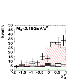
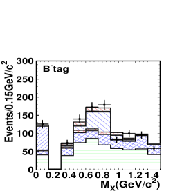
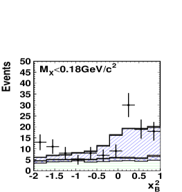
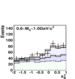
Figure 3: Projected $M_{X}$ distribution for $x_{B}^{2}>-2$ (left) and $x_{B}^{2}$ distributions for the mass region of $\pi$ ($M_{X}<0.18$GeV/$c^{2}$, middle) and $\rho$ ($0.6<M_{X}<1.0$GeV/$c^{2}$, right) in all $q^{2}$ region; points are data. Histogram components are $B^{0}\to\pi^{-}\ell^{+}\nu$ (red narrow $135^{\circ}$ hatching), $B^{0}\to\rho^{-}\ell^{+}\nu$ (red wide $45^{\circ}$ hatching), other $X_{u}\ell^{+}\nu$ from $B^{0}$ (red cross-hatching) and $B^{+}\to\pi^{0}\ell^{+}\nu$ (blue narrow $45^{\circ}$ hatching), $B^{+}\to\rho^{0}\ell^{+}\nu$ (blue wide $135^{\circ}$ hatching), other $X_{u}\ell^{+}\nu$ from $B^{+}$ (blue cross-hatching) and $B\bar{B}$ background (green horizontal hatching).

Figure 4 shows projections of the data, separated into three $q^{2}$ bins, $q^{2}<8$ GeV${}^{2}/c^{2}$, $8\leq q^{2}<16$ GeV${}^{2}/c^{2}$ and $q^{2}\geq 16$ GeV${}^{2}/c^{2}$. Here the normalizations of the other $B\to X_{u}\ell\nu$ and the $B\bar{B}$ background components are fixed to those obtained in the above fitting for the entire $q^{2}$ region. The extracted numbers of events for low/ medium/ high $q^{2}$ bins are, $N(B^{0}\to\pi^{-}\ell^{+}\nu)=64.8\pm 11.9~{}/~{}63.2\pm 12.4~{}/~{}40.6\pm 11.3$, $N(B^{0}\to\rho^{-}\ell^{+}\nu)=22.1\pm 8.0~{}/~{}53.2\pm 13.5~{}/~{}30.9\pm 16.0$, $N(B^{+}\to\pi^{0}\ell^{+}\nu)=18.1\pm 5.1~{}/~{}34.5\pm 8.3~{}/~{}18.6\pm 6.5$ and $N(B^{+}\to\rho^{0}\ell^{+}\nu)=47.2\pm 11.2~{}/~{}68.3\pm 16.5~{}/~{}32.5\pm 12.3$. Table 2 summarizes the extracted branching fractions. The branching fractions are calculated for each signal FF-model, where we take the average for cross-feed FF-models. The results are unfolded using the efficiency matrix $\epsilon(q^{2}_{\rm rec.},q^{2}_{\rm true})$ for the three $q^{2}$ intervals prepared for each signal FF-model. We calculate the total branching fraction by taking the sum of the partial branching fractions in the three $q^{2}$ intervals.

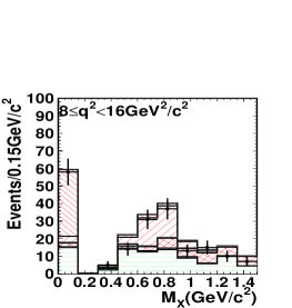
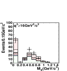
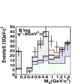
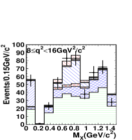
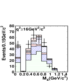
Figure 4: Projected $M_{X}$ distribution for $x_{B}^{2}>-2$ in each $q^{2}$ region; points are data. Histogram components are $B^{0}\to\pi^{-}\ell^{+}\nu$ (red narrow $135^{\circ}$ hatching), $B^{0}\to\rho^{-}\ell^{+}\nu$ (red wide $45^{\circ}$ hatching), other $X_{u}\ell^{+}\nu$ from $B^{0}$ (red cross-hatching) and $B^{+}\to\pi^{0}\ell^{+}\nu$ (blue narrow $45^{\circ}$ hatching), $B^{+}\to\rho^{0}\ell^{+}\nu$ (blue wide $135^{\circ}$ hatching), other $X_{u}\ell^{+}\nu$ from $B^{+}$ (blue cross-hatching) and $B\bar{B}$ background (green horizontal hatching).

Table 2: Extracted branching fractions for each signal mode with different FF models in units of 10^-4: the total branching fraction and the partial branching fractions in three $q^{2}$ intervals. $\chi^{2}/n$ and the associated probability for this $\chi^{2}$ indicate the quality of the fit for the FF shape to the observed $q^{2}$ distribution.

Mode	Model	${\mathcal{B}}_{\rm total}$	${\mathcal{B}}_{<8}$	${\mathcal{B}}_{8-16}$	${\mathcal{B}}_{\geq 16}$	$\chi^{2}/n$	$Prob.$
$\pi^{-}\ell^{+}\nu$	LCSR	$1.40\pm 0.19$	$0.52\pm 0.11$	$0.51\pm 0.11$	$0.36\pm 0.10$	0.4/2	0.81
	ISGW II	$1.36\pm 0.19$	$0.52\pm 0.11$	$0.48\pm 0.11$	$0.36\pm 0.10$	3.6/2	0.17
	UKQCD	$1.39\pm 0.19$	$0.53\pm 0.11$	$0.50\pm 0.11$	$0.36\pm 0.10$	0.2/2	0.89
	FNAL	$1.39\pm 0.19$	$0.52\pm 0.11$	$0.51\pm 0.11$	$0.36\pm 0.10$	0.3/2	0.86
	HPQCD	$1.39\pm 0.19$	$0.52\pm 0.11$	$0.50\pm 0.11$	$0.36\pm 0.10$	0.5/2	0.79
	Average	$1.38\pm 0.19$	$0.52\pm 0.11$	$0.50\pm 0.11$	$0.36\pm 0.10$	–	–
$\rho^{-}\ell^{+}\nu$	LCSR	$2.21\pm 0.54$	$0.48\pm 0.19$	$1.18\pm 0.33$	$0.55\pm 0.39$	2.4/2	0.43
	ISGW II	$2.09\pm 0.54$	$0.44\pm 0.17$	$1.14\pm 0.32$	$0.51\pm 0.39$	0.5/2	0.78
	UKQCD	$2.19\pm 0.54$	$0.48\pm 0.19$	$1.20\pm 0.33$	$0.51\pm 0.38$	1.7/2	0.43
	Melikhov	$2.20\pm 0.54$	$0.48\pm 0.19$	$1.22\pm 0.34$	$0.50\pm 0.37$	1.8/2	0.41
	Average	$2.17\pm 0.54$	$0.47\pm 0.19$	$1.19\pm 0.33$	$0.52\pm 0.38$	–	–
$\pi^{0}\ell^{+}\nu$	LCSR	$0.77\pm 0.14$	$0.19\pm 0.06$	$0.39\pm 0.10$	$0.20\pm 0.08$	2.9/2	0.24
	ISGW II	$0.77\pm 0.14$	$0.19\pm 0.06$	$0.39\pm 0.10$	$0.20\pm 0.08$	7.8/2	0.02
	UKQCD	$0.77\pm 0.14$	$0.19\pm 0.06$	$0.38\pm 0.10$	$0.20\pm 0.08$	2.5/2	0.28
	FNAL	$0.77\pm 0.14$	$0.19\pm 0.06$	$0.39\pm 0.10$	$0.20\pm 0.08$	2.8/2	0.25
	HPQCD	$0.77\pm 0.14$	$0.19\pm 0.06$	$0.39\pm 0.10$	$0.20\pm 0.08$	4.8/2	0.09
	Average	$0.77\pm 0.14$	$0.19\pm 0.06$	$0.39\pm 0.10$	$0.20\pm 0.08$	–	–
$\rho^{0}\ell^{+}\nu$	LCSR	$1.36\pm 0.23$	$0.43\pm 0.11$	$0.63\pm 0.16$	$0.29\pm 0.12$	0.9/2	0.64
	ISGW II	$1.29\pm 0.22$	$0.45\pm 0.11$	$0.57\pm 0.15$	$0.27\pm 0.12$	1.4/2	0.50
	UKQCD	$1.34\pm 0.23$	$0.45\pm 0.11$	$0.62\pm 0.16$	$0.28\pm 0.12$	0.2/2	0.91
	Melikhov	$1.35\pm 0.23$	$0.44\pm 0.11$	$0.63\pm 0.17$	$0.28\pm 0.12$	0.2/2	0.92
	Average	$1.33\pm 0.23$	$0.44\pm 0.11$	$0.61\pm 0.16$	$0.28\pm 0.12$	–	–

5 Systematic Errors

Tables 3 and 4 summarize the experimental systematic errors on the branching fractions. The experimental systematic errors can be categorized as originating from uncertainties in the signal reconstruction efficiency, the background estimation, and the normalization. The total experimental systematic error is the quadratic sum of all individual ones. We also consider the systematic error due to the dependence on the FF model.

The effect from the uncertainty on the signal reconstruction efficiency is evaluated based on the efficiency calibration with the $B_{\rm sig}\to D^{*}\ell^{+}\nu$ sample, discussed above. The error is taken to be that on the ratio of observed to expected number of the calibration signals (9.3% for $B^{0}\to\pi^{-}/\rho^{-}\ell^{+}\nu$, 9.2% for $B\to\pi^{0}/\rho^{0}\ell^{+}\nu$). This gives the largest contribution to the systematic error. Note that this error is dominated by the statistics of the calibration signals, as explained above. Therefore, accumulation of additional integrated luminosity in the future will help to reduce this uncertainty. We also include residual errors for the reconstruction of the signal side: 1% and 2% for the detection of each charged and neutral pion, respectively, and 2% for the charged pion selection and 2.1% for the lepton selection.

The systematic error due to the uncertainty on the inclusive branching fraction ${\mathcal{B}}(B\to X_{u}\ell\nu)$, which is used to constrain $B\to X_{u}\ell^{+}\nu$ background, is estimated by varying this parameter by its $\pm 1\sigma$ error. The uncertainty in the $B\bar{B}$ background shape after our pion multiplicity selection requirements ($N_{\pi^{+}}=1$ or $N_{\pi^{+}}=N_{\pi^{0}}=1$ for a $\bar{B^{0}}$ tag and $N_{\pi^{0}}=1$ or $N_{\pi^{+}}=N_{\pi^{-}}=1$ for a $B^{-}$ tag) is studied in the simulation by randomly removing charged tracks and $\pi^{0}$ according to the error in detection efficiency (1% for a charged track, 2% for $\pi^{0}$), and also by reassigning identified charged kaons as pions according to the uncertainty in the kaon identification efficiency (2%). The resultant changes in the extracted branching fractions are assigned as systematic errors. We find a significant uncertainty in the high $q^{2}$ region ($q^{2}>16$ GeV${}^{2}/c^{2}$) for $B\to\rho\ell^{+}\nu$ due to the poor signal-to-noise ratio. We also vary the fraction of $B\to D^{**}\ell\nu$ decays in the $B\bar{B}$ background MC by the error quoted in [21] to test the $B\to X_{c}\ell\nu$ model dependence in the $B\bar{B}$ background shape. To assess the uncertainty due to the production rate of $K_{L}^{0}$, we vary the production rate in the MC simulation by the uncertainty in the inclusive branching fraction for $B\to K^{0}~{}X$ quoted in [21].

For the normalization, we consider the uncertainty in the number of $B^{0}\bar{B^{0}}$ and $B^{+}B^{-}$ pairs: the ratio of $B^{+}B^{-}$ to $B^{0}\bar{B^{0}}$ pairs ($f_{+}/f_{0}$), $f_{+}/f_{0}=1.029\pm 0.035$  [23] , the mixing parameter ($\chi_{d}$), $\chi_{d}=0.186\pm 0.004$  [21], and the measured number of $B\bar{B}$ pairs ($N_{B\bar{B}}$, 1.1%).

Table 3: Summary of systematic errors (%) for ${\mathcal{B}}(B^{0}\to\pi^{-}/\rho^{-}\ell^{+}\nu)$.

	$B^{0}\to\pi^{-}\ell^{+}\nu$					$B^{0}\to\rho^{-}\ell^{+}\nu$
	$q^{2}$ interval (GeV${}^{2}/c^{2}$)					$q^{2}$ interval (GeV${}^{2}/c^{2}$)
Source	$q^{2}<8$	$8-16$	$\geq 16$	$<16$	all	$q^{2}<8$	$8-16$	$\geq 16$	$<16$	all
Tracking efficiency	1	1	1	1	1	1	1	1	1	1
$\pi^{0}$ reconstruction	–	–	–	–	–	2	2	2	2	2
Lepton identification	2.1	2.1	2.1	2.1	2.1	2.1	2.1	2.1	2.1	2.1
Kaon identification	2	2	2	2	2	2	2	2	2	2
$D^{*}\ell\nu$ calibration	9.3	9.3	9.3	9.3	9.3	9.3	9.3	9.3	9.3	9.3
$Br(X_{u}\ell\nu)$ in the fitting	0.8	2.4	1.8	1.6	1.4	4.8	3.9	23.8	1.9	7.1
$B\bar{B}$ background shape	1.1	2.2	2.8	1.2	1.3	3.8	2.9	17.0	3.0	6.1
$Br(D^{**}\ell\nu)$	1.0	1.5	0.2	1.2	0.9	0.5	0.3	2.5	0.3	0.8
$K_{L}^{0}$ production rate	0.1	0.3	0.4	0.2	0.3	1.0	0.7	2.9	0.8	1.3
$N_{B\overline{B}}$	1.1	1.1	1.1	1.1	1.1	1.1	1.1	1.1	1.1	1.1
$\it{f}_{+}/\it{f}_{0}$	1.7	1.7	1.7	1.7	1.7	1.7	1.7	1.7	1.7	1.7
$\chi_{d}$	2.2	2.2	2.2	2.2	2.2	2.2	2.2	2.2	2.2	2.2
exp. total	10.4	10.9	10.8	10.5	10.5	12.1	11.5	31.3	11.1	14.1
FF for signal	0.7	3.8	0.9	2.2	1.8	6.1	3.5	6.8	4.3	3.6
FF for cross-feed	1.8	2.1	1.5	1.9	1.4	0.5	0.7	2.4	0.6	1.0
FF total	1.9	4.3	1.7	2.9	2.3	6.1	3.6	7.2	4.3	3.7

Table 4: Summary of systematic errors (%) for ${\mathcal{B}}(B^{+}\to\pi^{0}/\rho^{0}\ell^{+}\nu)$.

	$B^{+}\to\pi^{0}\ell^{+}\nu$					$B^{+}\to\rho^{0}\ell^{+}\nu$
	$q^{2}$ interval (GeV${}^{2}/c^{2}$)					$q^{2}$ interval ( GeV${}^{2}/c^{2}$)
Source	$q^{2}<8$	$8-16$	$\geq 16$	$<16$	all	$q^{2}<8$	$8-16$	$\geq 16$	$<16$	all
Tracking efficiency	–	–	–	–	–	2	2	2	2	2
$\pi^{0}$ reconstruction	2	2	2	2	2	–	–	–	–	–
Lepton identification	2.1	2.1	2.1	2.1	2.1	2.1	2.1	2.1	2.1	2.1
Kaon identification	–	–	–	–	–	4	4	4	4	4
$D^{*}\ell\nu$ calibration	9.2	9.2	9.2	9.2	9.2	9.2	9.2	9.2	9.2	9.2
$Br(X_{u}\ell\nu)$ in the fitting	0.2	3.1	3.0	2.1	1.2	2.0	3.7	20.0	3.0	6.6
$B\bar{B}$ background shape	1.9	5.5	2.7	4.3	3.7	5.3	4.3	16.3	1.5	2.8
$Br(D^{**}\ell\nu)$	1.3	0.8	0.8	0.9	0.9	0.2	1.6	3.0	0.9	1.4
$K_{L}^{0}$ production rate	0.3	1.1	0.6	0.8	0.8	0.3	0.2	1.9	0.1	0.4
$N_{B\overline{B}}$	1.1	1.1	1.1	1.1	1.1	1.1	1.1	1.1	1.1	1.1
$\it{f}_{+}/\it{f}_{0}$	1.7	1.7	1.7	1.7	1.7	1.7	1.7	1.7	1.7	1.7
exp. total	10.1	11.8	10.7	11.0	10.7	12.1	12.2	28.1	11.2	12.9
FF for signal	1.2	0.5	1.3	0.3	0.2	2.1	7.1	3.9	3.7	3.5
FF for cross-feed	0.7	0.8	0.6	0.8	0.6	3.3	1.1	1.0	1.5	1.2
FF total	1.4	0.9	1.4	0.8	0.6	3.9	7.2	4.0	4.0	3.7

The dependence of the extracted branching fractions on the FF model has been studied by repeating the above fitting procedure with various FF models for the signal mode and also for the cross-feed mode ($B\to\pi\ell\nu\leftrightarrow B\to\rho\ell\nu$). We consider the models listed in Table 2. For the extracted ${\mathcal{B}}(B\to\pi^{-}\ell^{+}\nu~{}(\pi^{0}\ell^{+}\nu))$, the standard deviation among the models is $<1.7~{}(0.9)$% for $B\to\pi\ell^{+}\nu$ and $<1.9~{}(0.5)$% for $B\to\rho\ell^{+}\nu$. For ${\mathcal{B}}(B\to\rho^{-}\ell^{+}\nu~{}(\rho^{0}\ell^{+}\nu))$, the standard deviation is $<2.9~{}(3.6)$% for $B\to\rho\ell^{+}\nu$ and $<1.0~{}(1.3)$% for $B\to\pi\ell^{+}\nu$. The total error due to FF model dependence is the quadratic sum of the maximum variations with the signal and cross-feed FF models.

6 Results

Table 5 summarizes our measurements of the total and partial branching fractions for the four signal modes. Each branching fraction is obtained by taking the simple average of the values obtained from the FF models shown in Table 2. The errors shown in the table are statistical, experimental systematic, and model dependence due to form-factor uncertainties. The obtained branching fractions for $B^{0}\to\pi^{-}/\rho^{-}\ell^{+}\nu$ are consistent with the existing measurements by CLEO [6] and BaBar [9]. The overall uncertainty on our result for $B^{0}\to\pi^{-}\ell^{+}\nu$ (17%) is comparable to those on CLEO and BaBar results based on $\nu$-reconstruction. Our results for $B^{0}\to\rho^{-}\ell^{+}\nu$ have the smallest uncertainty.

Table 5: Summary of the obtained branching fractions. The errors are statistical, experimental systematic, and systematic due to form-factor uncertainties.

Modes	$q^{2}$ region (GeV${}^{2}/c^{2})$	Branching fraction ($\times 10^{-4}$)
$B^{0}\to\pi^{-}\ell^{+}\nu$	Total	$1.38\pm 0.19\pm 0.14\pm 0.03$
	$>16$	$0.36\pm 0.10\pm 0.04\pm 0.01$
	$<16$	$1.02\pm 0.16\pm 0.11\pm 0.03$
$B^{+}\to\pi^{0}\ell^{+}\nu$	Total	$0.77\pm 0.14\pm 0.08\pm 0.00$
	$>16$	$0.20\pm 0.08\pm 0.02\pm 0.00$
	$<16$	$0.57\pm 0.12\pm 0.06\pm 0.00$
$B^{0}\to\rho^{-}\ell^{+}\nu$	Total	$2.17\pm 0.54\pm 0.31\pm 0.08$
$B^{+}\to\rho^{0}\ell^{+}\nu$	Total	$1.33\pm 0.23\pm 0.17\pm 0.05$

Figure 5 presents the measured $q^{2}$ distributions for each signal mode, overlaid with the best fits of FF shapes to the data. To be self-consistent, the shape of a particular FF model is fit to the $q^{2}$ distribution extracted with the same FF model. The quality of the fit in terms of $\chi^{2}$ and the probability of $\chi^{2}$, shown in Table 2, may provide one way to discriminate among the models. From our results, the ISGW II model is disfavored for $B\to\pi\ell^{+}\nu$.

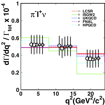
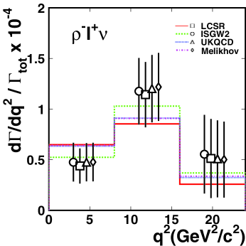
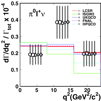
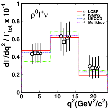
Figure 5: Extracted $q^{2}$ distribution. Data points are shown for different FF models used to estimate the detection efficiency. Lines are for the best fit of the FF shapes to the obtained $q^{2}$ distribution.

In this work, the $B^{0}\to\pi^{-}\ell^{+}\nu/B^{+}\to\pi^{0}\ell^{+}\nu$ and $B^{0}\to\rho^{-}\ell^{+}\nu/B^{+}\to\rho^{0}\ell^{+}\nu$ signals are extracted separately, which allows us to test the isospin relations. From the obtained branching fractions and the $B$ meson lifetimes in  [21], the ratios of decay rates are found to be,

$$\frac{\Gamma(B^{0}\to\pi^{-}\ell^{+}\nu)}{\Gamma(B^{+}\to\pi^{0}\ell^{+}\nu)}=(1.92\pm 0.43\pm 0.28),$$ (2)

$$\frac{\Gamma(B^{0}\to\rho^{-}\ell^{+}\nu)}{\Gamma(B^{+}\to\rho^{0}\ell^{+}\nu)}=(1.74\pm 0.53\pm 0.33),$$ (3)

where the first and second errors are statistical and systematic errors, respectively. Both ratios are found to be consistent with the isospin relations; $\Gamma(B^{0}\to\pi^{-}(\rho^{-})\ell^{+}\nu)=2\Gamma(B^{+}\to\pi^{0}(\rho^{0})\ell^{+}\nu)$.

The obtained branching fractions in Table 5 can be used to extract $|V_{ub}|$ using the relation,

$$|V_{ub}|=\sqrt{\frac{{\mathcal{B}}(B\to\pi\ell^{+}\nu)}{{\tilde{\Gamma}}_{thy}~{}\tau_{B}}},$$ (4)

where ${\tilde{\Gamma}}_{thy}$ is the form-factor normalization, predicted from theories. In Table 5, we list the partial branching fractions for $B\to\pi\ell^{+}\nu$ decays in the $q^{2}$ region above 16 GeV${}^{2}/c^{2}$, where the LQCD calculations are most reliable. The table provides also the results in the region below 16 GeV${}^{2}/c^{2}$, so that one can deduce $|V_{ub}|$ based on other approaches such as LCSR calculations [15, 16].

In this paper we calculate $|V_{ub}|$ based on the $B\to\pi\ell^{+}\nu$ data in the high $q^{2}$ region and the form factor predicted by recent unquenched LQCD calculations. Their predictions (${\tilde{\Gamma}}_{thy}$) for the $q^{2}\geq 16$ GeV${}^{2}/c^{2}$ region are ${\tilde{\Gamma}}_{thy}(B^{0}\to\pi^{-}\ell^{+}\nu)=1.83\pm 0.50$ ps^-1 (FNAL) [2] and ${\tilde{\Gamma}}_{thy}(B^{0}\to\pi^{-}\ell^{+}\nu)=1.46\pm 0.35$ ps^-1 (HPQCD) [3]. We use $\tau_{B^{0}}=1.532\pm 0.009$ ps and $\tau_{B^{+}}=1.638\pm 0.011$ ps  [21], and we use isospin symmetry to relate ${\tilde{\Gamma}}_{thy}$ for $B^{0}\to\pi^{-}$ and $B^{+}\to\pi^{0}$ transitions. The results for $B^{0}\to\pi^{-}\ell^{+}\nu$ and $B^{+}\to\pi^{0}\ell^{+}\nu$ are then averaged, weighted by their respective statistical errors.

Table 6: Summary of $|V_{ub}|$ obtained from the $B\to\pi\ell^{+}\nu$ data in the $q^{2}\geq 16$ GeV${}^{2}/c^{2}$ region. The first and second errors are experimental statistical and systematic errors, respectively. The third error stems from the error on ${\tilde{\Gamma}}_{thy}$ quoted by the LQCD authors.

Theory	${\tilde{\Gamma}}_{thy}$(ps-1)	Mode	$|V_{ub}|(\times 10^{-3})$
FNAL	$1.83\pm 0.50$	$\pi^{-}\ell^{+}\nu$	$3.59\pm 0.51\pm 0.20^{+0.62}_{-0.41}$
		$\pi^{0}\ell^{+}\nu$	$3.63\pm 0.70\pm 0.20^{+0.63}_{-0.41}$
		$\pi^{-}\ell^{+}\nu+\pi^{0}\ell^{+}\nu$	$3.60\pm 0.41\pm 0.20^{+0.62}_{-0.41}$
HPQCD	$1.46\pm 0.35$	$\pi^{-}\ell^{+}\nu$	$4.02\pm 0.57\pm 0.22^{+0.59}_{-0.41}$
		$\pi^{0}\ell^{+}\nu$	$4.06\pm 0.78\pm 0.22^{+0.60}_{-0.41}$
		$\pi^{-}\ell^{+}\nu+\pi^{0}\ell^{+}\nu$	$4.03\pm 0.46\pm 0.22^{+0.59}_{-0.41}$

Table 6 summarizes the results, where the first and second errors are the experimental statistical and systematic errors, respectively. The third error is based on the error on ${\tilde{\Gamma}}_{thy}$ quoted by the LQCD authors. These theoretical errors are asymmetric because we assign them by taking the variation in $|V_{ub}|$ when ${\tilde{\Gamma}}_{thy}$ is varied by the quoted errors. The values are in agreement with those from inclusive $B\to X_{u}\ell\nu$ decays [24].

To summarize, we have measured the branching fractions of the decays $B\to\pi\ell\nu$ and $B\to\rho\ell\nu$ in $2.75\times 10^{8}$ $B\bar{B}$ events using a method which tags one $B$ in the mode $B\to D^{(*)}\ell\nu$. Our results are consistent with previous measurements, and their precision is comparable to that of results from other experiments. The ratios of results for neutral and charged $B$ meson modes are found to be consistent with isospin. The partial rates are measured in three bins of $q^{2}$ and compared with distributions predicted by several theories. From the rate in the region $q^{2}\geq 16$ GeV${}^{2}/c^{2}$ and recent results from LQCD calculations, we extract $|V_{ub}|$:

$$|V_{ub}|_{(q^{2}\geq 16~{}{\rm GeV}^{2}/c^{2})}^{\pi^{-}\ell^{+}\nu+\pi^{0}\ell^{+}\nu} = (3.60\pm 0.41\pm 0.20^{+0.62}_{-0.41})\times 10^{-3}(\mbox{FNAL LQCD}),$$ (5)

$$|V_{ub}|_{(q^{2}\geq 16~{}{\rm GeV}^{2}/c^{2})}^{\pi^{-}\ell^{+}\nu+\pi^{0}\ell^{+}\nu} = (4.03\pm 0.46\pm 0.22^{+0.59}_{-0.41})\times 10^{-3}(\mbox{HPQCD LQCD}).$$ (6)

The experimental precision on these values is 13%, currently dominated by the statistical error of 11%. By accumulating more integrated luminosity, a measurement with errors below 10% is feasible. With improvements to unquenched LQCD calculations, the present method may provide a precise determination of $|V_{ub}|$.

We thank the KEKB group for the excellent operation of the accelerator, the KEK cryogenics group for the efficient operation of the solenoid, and the KEK computer group and the National Institute of Informatics for valuable computing and Super-SINET network support. We acknowledge support from the Ministry of Education, Culture, Sports, Science, and Technology of Japan and the Japan Society for the Promotion of Science; the Australian Research Council and the Australian Department of Education, Science and Training; the National Science Foundation of China and the Knowledge Innovation Program of Chinese Academy of Sciencies under contract No. 10575109 and IHEP-U-503; the Department of Science and Technology of India; the BK21 program of the Ministry of Education of Korea, and the CHEP SRC program and Basic Research program (grant No. R01-2005-000-10089-0) of the Korea Science and Engineering Foundation; the Polish State Committee for Scientific Research under contract No. 2P03B 01324; the Ministry of Science and Technology of the Russian Federation; the Slovenian Research Agency; the Swiss National Science Foundation; the National Science Council and the Ministry of Education of Taiwan; and the U.S. Department of Energy.

References

[1]
N. Cabibbo, Phys. Rev. Lett. 10, 531 (1963); M. Kobayashi and T. Maskawa, Prog. Theor. Phys. 49, 652 (1973).
[2]
M. Okamoto et al., Nucl.Phys.Proc.Suppl.140, 461 (2005).
[3]
E. Gulez et al. (HPQCD Collaboration), hep-lat/0601021 (2006).
[4]
J. P. Alexander et al. (CLEO Collaboration),
Phys. Rev. Lett. 77, 5000 (1996).
[5]
J. P. Alexander et al. (CLEO Collaboration),
Phys. Rev. D61, 052001 (2000).
[6]
S. B. Athar et al. (CLEO Collaboration),
Phys. Rev. D 68, 072003 (2003).
[7]
B. Aubert et al. (BaBar Collaboration),
Phys. Rev. Lett. 90, 181801 (2003).
[8]
C. Schwanda et al. (Belle Collaboration),
Phys. Rev. Lett. 93, 131803 (2004).
[9]
B. Aubert et al. (BaBar Collaboration),
Phys. Rev. D 72, 051102 (2005).
[10]
S. Kurokawa and E. Kikutani,
Nucl. Instr. and Meth. A 499, 1 (2003), and other papers included in
this volume.
[11]
A. Abashian et al. (Belle Collaboration),
Nucl. Instr. and Meth. A 479, 117 (2002).
[12] Y. Ushiroda (Belle SVD2 Group),
Nucl. Instr. and Meth.A 511 6 (2003).
[13]
R. Brun et al., GEANT3.21, CERN Report DD/EE/84-1 (1984).
[14]
D. Scora and N. Isgur, Phys. Rev. D 52, 2783 (1995).
[15]
P. Ball and R. Zwicky, Phys. Rev. D 71, 014015 (2005).
[16]
P. Ball and R. Zwicky, Phys. Rev. D 71, 014029 (2005).
[17]
L. Del Debbio, J. M. Flynn, L. Lellouch, and J. Nieves (UKQCD Collaboration),
Phys. Lett. B 416, 392 (1998).
[18]
D. Melikhov and B. Stech, Phys. Rev. D 62, 014006 (2000).
[19]
F. De Fazio and M. Neubert, JHEP 9906, 017 (1999).
[21]
S. Eidelman et al., Phys. Lett. B 592, 1 (2004) and 2005 partial
update for the 2006 edition available on the PDG WWW pages (URL: http://pdg.lbl.gov/).
[22]
H. Kakuno et al. (Belle Collaboration),
Phys. Rev. Lett 92, 071802 (2004);
the inclusive branching fraction used in the fitting is based on the
partial branching fraction GeV/ GeV) and a calculation of
shown in hep-ex/0408115.
[23]
Heavy Flavor Averaging Group, hep-ex/0505100
[24]
Heavy Flavor Averaging Group (HFAG), E. Barberio et al., hep-ex/0603003
and online update at http://www.slac.stanford.edu/xorg/hfag