CERN–PH-EP/2004-046

18 December 2003

DELPHI Collaboration

Abstract

The exclusive and semi-exclusive branching ratios of the $\tau$ lepton hadronic decay modes ( $h^{-}\nu_{\tau}$, $h^{-}\pi^{0}\nu_{\tau}$, $h^{-}\pi^{0}\pi^{0}\nu_{\tau}$, $h^{-}\geq\!2\pi^{0}\nu_{\tau}$, $h^{-}\geq\!3\pi^{0}\nu_{\tau}$, $2h^{-}h^{+}\nu_{\tau}$, $2h^{-}h^{+}\pi^{0}\nu_{\tau}$, $2h^{-}h^{+}\geq\!2\pi^{0}\nu_{\tau}$, $3h^{-}2h^{+}\nu_{\tau}$ and $3h^{-}2h^{+}\geq 1\pi^{0}\nu_{\tau}$) were measured with data from the DELPHI detector at LEP.

( Accepted by Euro. Phys. Journ. C. )

J.Abdallah${}^{\ref{LPNHE}}$, P.Abreu${}^{\ref{LIP}}$, W.Adam${}^{\ref{VIENNA}}$, P.Adzic${}^{\ref{DEMOKRITOS}}$, T.Albrecht${}^{\ref{KARLSRUHE}}$, T.Alderweireld${}^{\ref{AIM}}$, R.Alemany-Fernandez${}^{\ref{CERN}}$, T.Allmendinger${}^{\ref{KARLSRUHE}}$, P.P.Allport${}^{\ref{LIVERPOOL}}$, U.Amaldi${}^{\ref{MILANO2}}$, N.Amapane${}^{\ref{TORINO}}$, S.Amato${}^{\ref{UFRJ}}$, E.Anashkin${}^{\ref{PADOVA}}$, A.Andreazza${}^{\ref{MILANO}}$, S.Andringa${}^{\ref{LIP}}$, N.Anjos${}^{\ref{LIP}}$, P.Antilogus${}^{\ref{LPNHE}}$, W-D.Apel${}^{\ref{KARLSRUHE}}$, Y.Arnoud${}^{\ref{GRENOBLE}}$, S.Ask${}^{\ref{LUND}}$, B.Asman${}^{\ref{STOCKHOLM}}$, J.E.Augustin${}^{\ref{LPNHE}}$, A.Augustinus${}^{\ref{CERN}}$, P.Baillon${}^{\ref{CERN}}$, A.Ballestrero${}^{\ref{TORINOTH}}$, P.Bambade${}^{\ref{LAL}}$, R.Barbier${}^{\ref{LYON}}$, D.Bardin${}^{\ref{JINR}}$, G.J.Barker${}^{\ref{KARLSRUHE}}$, A.Baroncelli${}^{\ref{ROMA3}}$, M.Battaglia${}^{\ref{CERN}}$, M.Baubillier${}^{\ref{LPNHE}}$, K-H.Becks${}^{\ref{WUPPERTAL}}$, M.Begalli${}^{\ref{BRASIL}}$, A.Behrmann${}^{\ref{WUPPERTAL}}$, E.Ben-Haim${}^{\ref{LAL}}$, N.Benekos${}^{\ref{NTU-ATHENS}}$, A.Benvenuti${}^{\ref{BOLOGNA}}$, C.Berat${}^{\ref{GRENOBLE}}$, M.Berggren${}^{\ref{LPNHE}}$, L.Berntzon${}^{\ref{STOCKHOLM}}$, D.Bertrand${}^{\ref{AIM}}$, M.Besancon${}^{\ref{SACLAY}}$, N.Besson${}^{\ref{SACLAY}}$, D.Bloch${}^{\ref{CRN}}$, M.Blom${}^{\ref{NIKHEF}}$, M.Bluj${}^{\ref{WARSZAWA}}$, M.Bonesini${}^{\ref{MILANO2}}$, M.Boonekamp${}^{\ref{SACLAY}}$, P.S.L.Booth${}^{\ref{LIVERPOOL}}$, G.Borisov${}^{\ref{LANCASTER}}$, O.Botner${}^{\ref{UPPSALA}}$, B.Bouquet${}^{\ref{LAL}}$, T.J.V.Bowcock${}^{\ref{LIVERPOOL}}$, I.Boyko${}^{\ref{JINR}}$, M.Bracko${}^{\ref{SLOVENIJA}}$, R.Brenner${}^{\ref{UPPSALA}}$, E.Brodet${}^{\ref{OXFORD}}$, P.Bruckman${}^{\ref{KRAKOW1}}$, J.M.Brunet${}^{\ref{CDF}}$, L.Bugge${}^{\ref{OSLO}}$, P.Buschmann${}^{\ref{WUPPERTAL}}$, M.Calvi${}^{\ref{MILANO2}}$, T.Camporesi${}^{\ref{CERN}}$, V.Canale${}^{\ref{ROMA2}}$, F.Carena${}^{\ref{CERN}}$, N.Castro${}^{\ref{LIP}}$, F.Cavallo${}^{\ref{BOLOGNA}}$, M.Chapkin${}^{\ref{SERPUKHOV}}$, Ph.Charpentier${}^{\ref{CERN}}$, P.Checchia${}^{\ref{PADOVA}}$, R.Chierici${}^{\ref{CERN}}$, P.Chliapnikov${}^{\ref{SERPUKHOV}}$, J.Chudoba${}^{\ref{CERN}}$, S.U.Chung${}^{\ref{CERN}}$, K.Cieslik${}^{\ref{KRAKOW1}}$, P.Collins${}^{\ref{CERN}}$, R.Contri${}^{\ref{GENOVA}}$, G.Cosme${}^{\ref{LAL}}$, F.Cossutti${}^{\ref{TU}}$, M.J.Costa${}^{\ref{VALENCIA}}$, D.Crennell${}^{\ref{RAL}}$, J.Cuevas${}^{\ref{OVIEDO}}$, J.D’Hondt${}^{\ref{AIM}}$, J.Dalmau${}^{\ref{STOCKHOLM}}$, T.da Silva${}^{\ref{UFRJ}}$, W.Da Silva${}^{\ref{LPNHE}}$, G.Della Ricca${}^{\ref{TU}}$, A.De Angelis${}^{\ref{TU}}$, W.De Boer${}^{\ref{KARLSRUHE}}$, C.De Clercq${}^{\ref{AIM}}$, B.De Lotto${}^{\ref{TU}}$, N.De Maria${}^{\ref{TORINO}}$, A.De Min${}^{\ref{PADOVA}}$, L.de Paula${}^{\ref{UFRJ}}$, L.Di Ciaccio${}^{\ref{ROMA2}}$, A.Di Simone${}^{\ref{ROMA3}}$, K.Doroba${}^{\ref{WARSZAWA}}$, J.Drees${}^{\ref{WUPPERTAL},\ref{CERN}}$, M.Dris${}^{\ref{NTU-ATHENS}}$, G.Eigen${}^{\ref{BERGEN}}$, T.Ekelof${}^{\ref{UPPSALA}}$, M.Ellert${}^{\ref{UPPSALA}}$, M.Elsing${}^{\ref{CERN}}$, M.C.Espirito Santo${}^{\ref{LIP}}$, G.Fanourakis${}^{\ref{DEMOKRITOS}}$, D.Fassouliotis${}^{\ref{DEMOKRITOS},\ref{ATHENS}}$, M.Feindt${}^{\ref{KARLSRUHE}}$, J.Fernandez${}^{\ref{SANTANDER}}$, A.Ferrer${}^{\ref{VALENCIA}}$, F.Ferro${}^{\ref{GENOVA}}$, U.Flagmeyer${}^{\ref{WUPPERTAL}}$, H.Foeth${}^{\ref{CERN}}$, E.Fokitis${}^{\ref{NTU-ATHENS}}$, F.Fulda-Quenzer${}^{\ref{LAL}}$, J.Fuster${}^{\ref{VALENCIA}}$, M.Gandelman${}^{\ref{UFRJ}}$, C.Garcia${}^{\ref{VALENCIA}}$, Ph.Gavillet${}^{\ref{CERN}}$, E.Gazis${}^{\ref{NTU-ATHENS}}$, R.Gokieli${}^{\ref{CERN},\ref{WARSZAWA}}$, B.Golob${}^{\ref{SLOVENIJA}}$, G.Gomez-Ceballos${}^{\ref{SANTANDER}}$, P.Goncalves${}^{\ref{LIP}}$, E.Graziani${}^{\ref{ROMA3}}$, G.Grosdidier${}^{\ref{LAL}}$, K.Grzelak${}^{\ref{WARSZAWA}}$, J.Guy${}^{\ref{RAL}}$, C.Haag${}^{\ref{KARLSRUHE}}$, A.Hallgren${}^{\ref{UPPSALA}}$, K.Hamacher${}^{\ref{WUPPERTAL}}$, K.Hamilton${}^{\ref{OXFORD}}$, S.Haug${}^{\ref{OSLO}}$, F.Hauler${}^{\ref{KARLSRUHE}}$, V.Hedberg${}^{\ref{LUND}}$, M.Hennecke${}^{\ref{KARLSRUHE}}$, H.Herr${}^{\ref{CERN}}$, J.Hoffman${}^{\ref{WARSZAWA}}$, S-O.Holmgren${}^{\ref{STOCKHOLM}}$, P.J.Holt${}^{\ref{CERN}}$, M.A.Houlden${}^{\ref{LIVERPOOL}}$, K.Hultqvist${}^{\ref{STOCKHOLM}}$, J.N.Jackson${}^{\ref{LIVERPOOL}}$, G.Jarlskog${}^{\ref{LUND}}$, P.Jarry${}^{\ref{SACLAY}}$, D.Jeans${}^{\ref{OXFORD}}$, E.K.Johansson${}^{\ref{STOCKHOLM}}$, P.D.Johansson${}^{\ref{STOCKHOLM}}$, P.Jonsson${}^{\ref{LYON}}$, C.Joram${}^{\ref{CERN}}$, L.Jungermann${}^{\ref{KARLSRUHE}}$, F.Kapusta${}^{\ref{LPNHE}}$, S.Katsanevas${}^{\ref{LYON}}$, E.Katsoufis${}^{\ref{NTU-ATHENS}}$, G.Kernel${}^{\ref{SLOVENIJA}}$, B.P.Kersevan${}^{\ref{CERN},\ref{SLOVENIJA}}$, U.Kerzel${}^{\ref{KARLSRUHE}}$, A.Kiiskinen${}^{\ref{HELSINKI}}$, B.T.King${}^{\ref{LIVERPOOL}}$, N.J.Kjaer${}^{\ref{CERN}}$, P.Kluit${}^{\ref{NIKHEF}}$, P.Kokkinias${}^{\ref{DEMOKRITOS}}$, C.Kourkoumelis${}^{\ref{ATHENS}}$, O.Kouznetsov${}^{\ref{JINR}}$, Z.Krumstein${}^{\ref{JINR}}$, M.Kucharczyk${}^{\ref{KRAKOW1}}$, J.Lamsa${}^{\ref{AMES}}$, G.Leder${}^{\ref{VIENNA}}$, F.Ledroit${}^{\ref{GRENOBLE}}$, L.Leinonen${}^{\ref{STOCKHOLM}}$, R.Leitner${}^{\ref{NC}}$, J.Lemonne${}^{\ref{AIM}}$, V.Lepeltier${}^{\ref{LAL}}$, T.Lesiak${}^{\ref{KRAKOW1}}$, W.Liebig${}^{\ref{WUPPERTAL}}$, D.Liko${}^{\ref{VIENNA}}$, A.Lipniacka${}^{\ref{STOCKHOLM}}$, J.H.Lopes${}^{\ref{UFRJ}}$, J.M.Lopez${}^{\ref{OVIEDO}}$, D.Loukas${}^{\ref{DEMOKRITOS}}$, P.Lutz${}^{\ref{SACLAY}}$, L.Lyons${}^{\ref{OXFORD}}$, J.MacNaughton${}^{\ref{VIENNA}}$, A.Malek${}^{\ref{WUPPERTAL}}$, S.Maltezos${}^{\ref{NTU-ATHENS}}$, F.Mandl${}^{\ref{VIENNA}}$, J.Marco${}^{\ref{SANTANDER}}$, R.Marco${}^{\ref{SANTANDER}}$, B.Marechal${}^{\ref{UFRJ}}$, M.Margoni${}^{\ref{PADOVA}}$, J-C.Marin${}^{\ref{CERN}}$, C.Mariotti${}^{\ref{CERN}}$, A.Markou${}^{\ref{DEMOKRITOS}}$, C.Martinez-Rivero${}^{\ref{SANTANDER}}$, J.Masik${}^{\ref{FZU}}$, N.Mastroyiannopoulos${}^{\ref{DEMOKRITOS}}$, F.Matorras${}^{\ref{SANTANDER}}$, C.Matteuzzi${}^{\ref{MILANO2}}$, F.Mazzucato${}^{\ref{PADOVA}}$, M.Mazzucato${}^{\ref{PADOVA}}$, R.Mc Nulty${}^{\ref{LIVERPOOL}}$, C.Meroni${}^{\ref{MILANO}}$, E.Migliore${}^{\ref{TORINO}}$, W.Mitaroff${}^{\ref{VIENNA}}$, U.Mjoernmark${}^{\ref{LUND}}$, T.Moa${}^{\ref{STOCKHOLM}}$, M.Moch${}^{\ref{KARLSRUHE}}$, K.Moenig${}^{\ref{CERN},\ref{DESY}}$, R.Monge${}^{\ref{GENOVA}}$, J.Montenegro${}^{\ref{NIKHEF}}$, D.Moraes${}^{\ref{UFRJ}}$, S.Moreno${}^{\ref{LIP}}$, P.Morettini${}^{\ref{GENOVA}}$, U.Mueller${}^{\ref{WUPPERTAL}}$, K.Muenich${}^{\ref{WUPPERTAL}}$, M.Mulders${}^{\ref{NIKHEF}}$, L.Mundim${}^{\ref{BRASIL}}$, W.Murray${}^{\ref{RAL}}$, B.Muryn${}^{\ref{KRAKOW2}}$, G.Myatt${}^{\ref{OXFORD}}$, T.Myklebust${}^{\ref{OSLO}}$, M.Nassiakou${}^{\ref{DEMOKRITOS}}$, F.Navarria${}^{\ref{BOLOGNA}}$, K.Nawrocki${}^{\ref{WARSZAWA}}$, R.Nicolaidou${}^{\ref{SACLAY}}$, M.Nikolenko${}^{\ref{JINR},\ref{CRN}}$, A.Oblakowska-Mucha${}^{\ref{KRAKOW2}}$, V.Obraztsov${}^{\ref{SERPUKHOV}}$, A.Olshevski${}^{\ref{JINR}}$, A.Onofre${}^{\ref{LIP}}$, R.Orava${}^{\ref{HELSINKI}}$, K.Osterberg${}^{\ref{HELSINKI}}$, A.Ouraou${}^{\ref{SACLAY}}$, A.Oyanguren${}^{\ref{VALENCIA}}$, M.Paganoni${}^{\ref{MILANO2}}$, S.Paiano${}^{\ref{BOLOGNA}}$, J.P.Palacios${}^{\ref{LIVERPOOL}}$, H.Palka${}^{\ref{KRAKOW1}}$, Th.D.Papadopoulou${}^{\ref{NTU-ATHENS}}$, L.Pape${}^{\ref{CERN}}$, C.Parkes${}^{\ref{GLASGOW}}$, F.Parodi${}^{\ref{GENOVA}}$, U.Parzefall${}^{\ref{CERN}}$, A.Passeri${}^{\ref{ROMA3}}$, O.Passon${}^{\ref{WUPPERTAL}}$, L.Peralta${}^{\ref{LIP}}$, V.Perepelitsa${}^{\ref{VALENCIA}}$, A.Perrotta${}^{\ref{BOLOGNA}}$, A.Petrolini${}^{\ref{GENOVA}}$, J.Piedra${}^{\ref{SANTANDER}}$, L.Pieri${}^{\ref{ROMA3}}$, F.Pierre${}^{\ref{SACLAY}}$, M.Pimenta${}^{\ref{LIP}}$, E.Piotto${}^{\ref{CERN}}$, T.Podobnik${}^{\ref{SLOVENIJA}}$, V.Poireau${}^{\ref{CERN}}$, M.E.Pol${}^{\ref{BRASIL}}$, G.Polok${}^{\ref{KRAKOW1}}$, V.Pozdniakov${}^{\ref{JINR}}$, N.Pukhaeva${}^{\ref{AIM},\ref{JINR}}$, A.Pullia${}^{\ref{MILANO2}}$, J.Rames${}^{\ref{FZU}}$, A.Read${}^{\ref{OSLO}}$, P.Rebecchi${}^{\ref{CERN}}$, J.Rehn${}^{\ref{KARLSRUHE}}$, D.Reid${}^{\ref{NIKHEF}}$, R.Reinhardt${}^{\ref{WUPPERTAL}}$, P.Renton${}^{\ref{OXFORD}}$, F.Richard${}^{\ref{LAL}}$, J.Ridky${}^{\ref{FZU}}$, M.Rivero${}^{\ref{SANTANDER}}$, D.Rodriguez${}^{\ref{SANTANDER}}$, A.Romero${}^{\ref{TORINO}}$, P.Ronchese${}^{\ref{PADOVA}}$, P.Roudeau${}^{\ref{LAL}}$, T.Rovelli${}^{\ref{BOLOGNA}}$, V.Ruhlmann-Kleider${}^{\ref{SACLAY}}$, D.Ryabtchikov${}^{\ref{SERPUKHOV}}$, A.Sadovsky${}^{\ref{JINR}}$, L.Salmi${}^{\ref{HELSINKI}}$, J.Salt${}^{\ref{VALENCIA}}$, C.Sander${}^{\ref{KARLSRUHE}}$, A.Savoy-Navarro${}^{\ref{LPNHE}}$, U.Schwickerath${}^{\ref{CERN}}$, A.Segar${}^{\ref{OXFORD}}$, R.Sekulin${}^{\ref{RAL}}$, M.Siebel${}^{\ref{WUPPERTAL}}$, A.Sisakian${}^{\ref{JINR}}$, G.Smadja${}^{\ref{LYON}}$, O.Smirnova${}^{\ref{LUND}}$, A.Sokolov${}^{\ref{SERPUKHOV}}$, A.Sopczak${}^{\ref{LANCASTER}}$, R.Sosnowski${}^{\ref{WARSZAWA}}$, T.Spassov${}^{\ref{CERN}}$, M.Stanitzki${}^{\ref{KARLSRUHE}}$, A.Stocchi${}^{\ref{LAL}}$, J.Strauss${}^{\ref{VIENNA}}$, B.Stugu${}^{\ref{BERGEN}}$, M.Szczekowski${}^{\ref{WARSZAWA}}$, M.Szeptycka${}^{\ref{WARSZAWA}}$, T.Szumlak${}^{\ref{KRAKOW2}}$, T.Tabarelli${}^{\ref{MILANO2}}$, A.C.Taffard${}^{\ref{LIVERPOOL}}$, F.Tegenfeldt${}^{\ref{UPPSALA}}$, J.Timmermans${}^{\ref{NIKHEF}}$, L.Tkatchev${}^{\ref{JINR}}$, M.Tobin${}^{\ref{LIVERPOOL}}$, S.Todorovova${}^{\ref{FZU}}$, B.Tome${}^{\ref{LIP}}$, A.Tonazzo${}^{\ref{MILANO2}}$, P.Tortosa${}^{\ref{VALENCIA}}$, P.Travnicek${}^{\ref{FZU}}$, D.Treille${}^{\ref{CERN}}$, G.Tristram${}^{\ref{CDF}}$, M.Trochimczuk${}^{\ref{WARSZAWA}}$, C.Troncon${}^{\ref{MILANO}}$, M-L.Turluer${}^{\ref{SACLAY}}$, I.A.Tyapkin${}^{\ref{JINR}}$, P.Tyapkin${}^{\ref{JINR}}$, S.Tzamarias${}^{\ref{DEMOKRITOS}}$, V.Uvarov${}^{\ref{SERPUKHOV}}$, G.Valenti${}^{\ref{BOLOGNA}}$, P.Van Dam${}^{\ref{NIKHEF}}$, J.Van Eldik${}^{\ref{CERN}}$, A.Van Lysebetten${}^{\ref{AIM}}$, N.van Remortel${}^{\ref{AIM}}$, I.Van Vulpen${}^{\ref{CERN}}$, G.Vegni${}^{\ref{MILANO}}$, F.Veloso${}^{\ref{LIP}}$, W.Venus${}^{\ref{RAL}}$, P.Verdier${}^{\ref{LYON}}$, V.Verzi${}^{\ref{ROMA2}}$, D.Vilanova${}^{\ref{SACLAY}}$, L.Vitale${}^{\ref{TU}}$, V.Vrba${}^{\ref{FZU}}$, H.Wahlen${}^{\ref{WUPPERTAL}}$, A.J.Washbrook${}^{\ref{LIVERPOOL}}$, C.Weiser${}^{\ref{KARLSRUHE}}$, D.Wicke${}^{\ref{CERN}}$, J.Wickens${}^{\ref{AIM}}$, G.Wilkinson${}^{\ref{OXFORD}}$, M.Winter${}^{\ref{CRN}}$, M.Witek${}^{\ref{KRAKOW1}}$, O.Yushchenko${}^{\ref{SERPUKHOV}}$, A.Zalewska${}^{\ref{KRAKOW1}}$, P.Zalewski${}^{\ref{WARSZAWA}}$, D.Zavrtanik${}^{\ref{SLOVENIJA}}$, V.Zhuravlov${}^{\ref{JINR}}$, N.I.Zimin${}^{\ref{JINR}}$, A.Zintchenko${}^{\ref{JINR}}$, M.Zupan${}^{\ref{DEMOKRITOS}}$

1 Introduction

The $\tau$ lepton, discovered in 1975 [1], is the only lepton which is sufficiently heavy to decay to final states containing hadrons. Predictions for the properties of such a heavy lepton have been made well in advance of its discovery [2]. The taus produce intermediate and final-state hadrons with lower backgrounds than most other low energy processes.

This paper describes a measurement of the decay rates of the $\tau$ lepton to the different hadronic final states as a function of both the charged-hadron and neutral-pion multiplicities, with no particle identification performed on the charged hadrons. Samples of different $\tau$-decay final states have been selected using both “sequential cuts” methods and neural networks. These analyses were complementary, allowing cross-checks of the results and their uncertainties.

The DELPHI detector and data sample are described in Section 2. The method used to determine the branching ratios is described in section 3. The techniques used to separate charged leptons from hadrons are outlined in Section 4.1. Section 4.2 describes the reconstruction of photons and neutral pions. The selection of ${\rm e}^{+}{\rm e}^{-}\rightarrow\tau^{+}\tau^{-}$ events is outlined in Section 5 and the isolated $\tau$-decays are classified according to their charged-particle multiplicity in Section 6. The selection of $\tau$-decays as a function of the neutral pion multiplicity is described in Section 7 and the associated systematic uncertainties on the measured branching ratios are discussed in Section 8. Section 9 presents the results and conclusions are drawn in Section 10.

DELPHI has previously published results on some of the decay modes measured here using the 1990 data sample [3]. This paper replaces those low-statistics results. Similar analyses performed by other LEP experiments can be found in  [4].

2 The DELPHI Detector and data sample

The DELPHI detector and its performance are described in detail in [5, 6]. The components relevant to this analysis are summarised below. Unless specified otherwise, they covered the full solid angle of the barrel region used in this analysis ($43^{\circ}<\theta<137^{\circ}$) and lay in a 1.2 Tesla solenoidal magnetic field parallel to the beam.

The charged-particle track reconstruction was based on four different detector components. The principal track reconstruction device was the Time Projection Chamber (TPC), a large drift chamber covering the radial region 35 cm $<$ r $<$ 111 cm. To enhance the precision of the TPC measurement, track reconstruction was supplemented by a three-layer silicon Vertex Detector (VD) at radii between 6 and 12 cm, an Inner Detector (ID) between 12 and 28 cm and the Outer Detector (OD) at radii between 197 and 206 cm from the z-axis. The TPC also provided up to 192 ionisation measurements per charged particle track, useful for electron/hadron separation. It had boundary regions between read-out sectors every $60^{\circ}$ in $\phi$ which were about $1^{\circ}$ wide and which were covered by the VD, ID, and OD.

The main device for $\gamma$ and $\pi^{0}$ reconstruction and electron/hadron separation, the High density Projection Chamber (HPC) lay between radii of 208 cm and 260 cm. It consisted of 40 layers of 3 mm thick lead interspersed with 8 mm thick layers of gas sampling volume, amounting to a minimum of about 18 radiation lengths. In the gas layers the ionising particles in a shower produced electrons which drifted in an electric field into wire chambers. In these wire chambers the induced signal on cathode pads gave a measurement of the deposited charge with sampling granularity of 10 mrad $\times$ 2 mrad $\times$ 1.0 $X_{0}$ in $\phi$ $\times$ $\theta$ $\times$ r in the inner 4 radiation lengths and provided up to nine longitudinal samplings of the energy deposition in a shower. The spatial precision for the starting point of an electromagnetic shower was 1 mrad in $\theta$ and 2 mrad in $\phi$. The energy resolution was $\Delta E/E=0.31/E^{0.44}\oplus 0.027$.

The Hadron Calorimeter (HCAL) was the instrumented flux return of the magnet. It was longitudinally segmented into 20 layers of iron and limited streamer tubes. The tubes were grouped to give four longitudinal segments in the readout, with a granularity of $3.75^{\circ}$ $\times$ $2.96^{\circ}$ in $\phi$$\times$$\theta$. Between the 18th and 19th HCAL layers and also outside the whole calorimeter, there were drift chambers for detecting the muons which were expected to penetrate the whole HCAL. The barrel muon chambers (MUB) covered the range $|\cos\!\theta|\!<\!0.602$ while most azimuthal zones in the range $0.602\!<\!|\cos\!\theta|$ were covered by forward muon chambers (MUF).

The Ring-Imaging Cherenkov detector (RICH), although not used in this analysis, had an important effect on the performance of the calorimetry as it contained the majority of the material in the DELPHI barrel region. Lying between the TPC and OD in radius, it covered the complete polar angle region of this analysis. The amount of material for particles of perpendicular incidence was equivalent to 0.6 radiation lengths and 0.15 nuclear interaction lengths.

The data were collected in the years 1992 to 1995, at centre-of-mass energies $\sqrt{s}$ between 89 and 93 GeV on or near to the Z resonance. It was required that the VD, TPC, HPC, MUB and HCAL subdetectors be fully operational. The integrated luminosity of the data sample was 135 pb^-1 of which about 100 pb^-1 was taken at $\sqrt{s}\approx$ 91.3 GeV, near the maximum of the Z production cross-section.

Selection requirements were studied on simulated event samples after a detailed simulation of the detector response [6] and reconstruction by the same program as the real data. Samples were simulated for the different detector conditions and centre-of-mass energies in every year of data taking and amounted to about 16 times the recorded luminosities. The Monte Carlo event generators used were: KORALZ 4.0 [7] for ${\rm e}^{+}{\rm e}^{-}\rightarrow\tau^{+}\tau^{-}$ events; DYMU3 [8] for ${\rm e}^{+}{\rm e}^{-}\rightarrow\mu^{+}\mu^{-}$ events; BABAMC [9] and BHWIDE [10] for ${\rm e}^{+}{\rm e}^{-}\rightarrow{\rm e}^{+}{\rm e}^{-}$ events; JETSET 7.3 [11] for ${\rm e}^{+}{\rm e}^{-}\rightarrow{\rm q}\bar{\rm q}$ events; BDK [12] for four-lepton final states; TWOGAM [13] for ${\rm e}^{+}{\rm e}^{-}\to{\rm e}^{+}{\rm e}^{-}{\rm q}\bar{\rm q}$ events. The KORALZ generator incorporated the TAUOLA2.5 [14] package for modelling $\tau$-decays.

3 Method

In an initial step, $\tau$-decays were selected according to their charged-particle multiplicity from a high-purity Z$\to\tau^{+}\tau^{-}$ event sample. In decays containing only one charged particle, this particle can be either an electron, muon or hadron. In higher charged-particle multiplicity decays the initial charged particles are hadrons.

After rejection of one-prong decays containing muons and electrons the following exclusive and semi-exclusive $\tau$ decay modes have been isolated and their branching ratios measured:

• Charged multiplicity one:
  $h^{-}\nu_{\tau}$,    $h^{-}\pi^{0}\nu_{\tau}$,    $h^{-}2\pi^{0}\nu_{\tau}$,     $h^{-}\geq 3\pi^{0}\nu_{\tau}$;

• Charged multiplicity three:
  $2h^{-}h^{+}\nu_{\tau}$,     $2h^{-}h^{+}\pi^{0}\nu_{\tau}$,     $2h^{-}h^{+}\geq 2\pi^{0}\nu_{\tau}$;

• Charged multiplicity five:
  $3h^{-}2h^{+}\nu_{\tau}$,     $3h^{-}2h^{+}\geq 1\pi^{0}\nu_{\tau}$.

where $h$ is either a $\pi$ or $K$ meson. The charge conjugate decays were also included.

The $\pi^{0}$ mesons were detected and reconstructed via the photons produced in the decay $\pi^{0}\to\gamma\gamma$. This $\pi^{0}$ decay mode has a branching ratio of (98.798$\pm$0.032)%, the remainder decaying through the Dalitz process $\pi^{0}\to\gamma{\rm e}^{+}{\rm e}^{-}$. Most of these were also correctly identified with the conversion rejection algorithm, and the fraction lost was a contribution to the inefficiency.

In the definition of these channels the presence of neutral kaons (reconstructed or not) was not considered. For example the decay $h^{-}\nu_{\tau}$, included channels with one charged hadron and none, one or more neutral kaons. The presence of neutral kaons did not significantly affect the selection efficiency, but was accounted for in the analysis.

Two complementary analyses were performed on each of the samples of charged multiplicity one and three $\tau$-decays. One analysis was based on sequential cuts and the other on neural networks. The $\tau$-decays were classified as a function of the $\pi^{0}$ multiplicity and the branching ratios were obtained taking into account statistical and systematic correlations. Only a sequential cuts analysis was performed for $\tau$-decays with charged multiplicity of five.

The branching ratios were measured simultaneously with the following procedure. Candidate $\tau$-decays can be classified using an estimator such as the maximum output neuron from a neural network or the set of cuts of the sequential analysis. On real data all decays are assigned to the different classes, providing the total number of events in each class: $N_{i,obs}$. On simulated data, a selection-probability matrix $M_{ij}$ can be obtained, representing the probability for decay mode $j$ to be classified as decay mode $i$. This matrix could be diagonal, but in fact most of the off-diagonal terms are non-zero. To obtain the Branching Ratios $B_{j}$, a maximum-likelihood fit can then be performed to constrain the predicted number, $N_{i,pred}$, of decays in class $i$ to $N_{i,obs}$ . $N_{i,pred}$ is given by:

$$N_{i,pred}=N_{\tau}\sum_{j=1}^{n_{c}}M_{ij}\epsilon_{j}B_{j}+N_{i,bkg}~{},$$ (1)

where $N_{\tau}$ is the total number of produced $\tau$ particles, which is left as a free parameter in the fit, $\epsilon_{j}$ is the efficiency for decay mode $j$ of the $\tau^{+}\tau^{-}$ selection, $N_{i,bkg}$ is the estimated background in class $i$ due to non-$\tau^{+}\tau^{-}$ events, and $n_{c}$ is the number of classes, synonymous with the number of decay modes if all decays are classified. In this analysis not all candidate $\tau$-decays were classified as a minimum level was required on the maximum output neuron of the neural network. Taking into account the track multiplicity, this led to three additional classes, corresponding to those decays which were unclassified. Having three classes instead of just one for all the unclassified modes, does not improve the precision on the measurement, but gives additional information on the comparison of topological and exclusive branching ratios.

If we do not take into account these three extra classes, the problem is undetermined, since there are $n_{c}+1$ unknowns (the $n_{c}$ branching ratios and $N_{\tau}$) and only $n_{c}$ measurements. The inclusion of these three classes, corresponding to the events not assigned to any given class, does not help, because, despite having three additional measurements, the equations are nearly degenerate (the matrix is almost singular) and the resulting fit is highly unstable. We avoid the problem by setting an additional constraint that all the branching ratios add to 1. In many previous measurements an alternative procedure is proposed, which is not correct in the case of multiple branching ratios. Here $N_{\tau}$ is obtained from the selected $\tau$ events, together with the expected efficiency ($\epsilon_{\tau\tau}$) and background ($b$), with the expression $N_{\tau}=2\cdot\frac{N_{\tau\tau}}{\epsilon_{\tau\tau}}\cdot(1-b)$. However, this expression needs to assume a priori the branching ratios to estimate the $\tau\tau$ selection efficiency and nevertheless also makes an implicit assumption on the sum of branching ratios when computing that efficiency. With the method described here, unexpected decays could affect the goodness of the fit through its $\chi^{2}$ and in particular, with an excess in the extra classes mentioned above.

4 Particle identification and detector calibration

The detector response was studied using simulation together with test samples of real data where the identity and momentum of the particles was unambiguously known. Examples of such samples consisted of ${\rm e}^{+}{\rm e}^{-}\rightarrow{\rm e}^{+}{\rm e}^{-}$ and ${\rm e}^{+}{\rm e}^{-}\rightarrow\mu^{+}\mu^{-}$ events, the radiative processes ${\rm e}^{+}{\rm e}^{-}\rightarrow{\rm e}^{+}{\rm e}^{-}\gamma$ and ${\rm e}^{+}{\rm e}^{-}\rightarrow\mu^{+}\mu^{-}\gamma$ and Compton events selected using kinematic constraints. Tau-decay test samples, which were selected taking advantage of the redundancy of the detector, were also used. An example is $\tau\rightarrow h({\mathrm{n}}\pi^{0})\nu$, (n$>$0), selected by tagging the $\pi^{0}$ decay in the HPC. This gave a pure sample of charged hadrons to test the response of the calorimetry, muon chambers, and ionisation loss in the TPC. The decays $\tau\rightarrow\mu\nu\nu$ selected with the calorimeters checked the muon chambers response and the TPC ionisation loss. Various test samples were used to calibrate the response of the model of the detector in the simulation program and where necessary to correct observed discrepancies.

Further details of electron, muon and charged-hadron separation in $\tau$-decays can be found in the analysis of the $\tau$ leptonic branching ratios [15].

4.1 Charged particles

4.1.1 Tracking

The precision on the component of the momentum transverse to the beam direction, $p_{t}$, obtained with the DELPHI tracking detectors was $\Delta(1/p_{t})=0.0008\rm{(GeV/\mathrm{c})^{-1}}$ for particles with momentum close to 45 GeV/c. Calibration of the momentum measurement was performed with ${\rm e}^{+}{\rm e}^{-}\rightarrow\mu^{+}\mu^{-}$ events. For lower momenta the masses of the $K^{0}_{s}$ and $\Lambda$ were reconstructed. For intermediate momenta three body decays (${\rm e}^{+}{\rm e}^{-}\rightarrow\mu^{+}\mu^{-}\gamma$ and ${\rm e}^{+}{\rm e}^{-}\rightarrow{\rm e}^{+}{\rm e}^{-}\gamma$) were used. In these cases, the true energy of the particles can be calculated to a good precision from energy and momentum conservation, using the accurate measurement of the particle direction only. The combination of all these methods gives an absolute momentum scale to a precision of 0.2% over the full momentum range.

Some 3% of hadrons reinteract inelastically with the detector material before the TPC. These were reconstructed with an algorithm which was designed to find secondary reinteraction vertices using the tracks from outgoing charged particles produced in nuclear interactions. This is described in detail in the DELPHI analysis of the $\tau$ topological Branching Ratios [16], where the efficiency of the algorithm, as well as the amount of material in the detector in terms of nuclear interaction lengths, were studied. The efficiency in the data was found to agree well with the simulation prediction while there was an overestimate by about 10% in the simulation of the number of nuclear interaction lengths before the TPC gas volume. The correction factors obtained have been applied via reweighting techniques.

4.1.2 TPC ionisation measurement

The energy loss per unit path length due to ionisation, $dE/dx$, of a charged particle traveling through the TPC gave good separation between electrons and charged pions, particularly in the low momentum range. The $dE/dx$ pull variable, $\prod^{j}_{dE/dx}$, for a particular particle hypothesis ($j$ = e,$\pi$,K,p) is defined as

$${\textstyle\prod^{j}_{dE/dx}}=\frac{{dE/dx}_{meas}-{dE/dx}_{exp}(j)}{\sigma(dE/dx)}~{}~{},$$ (2)

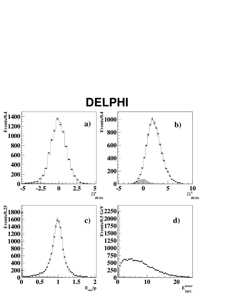
Figure 1: Distributions for electron test samples in $\tau$-decays : a) the variable $\Pi_{dE/dx}^{\rm e}$ ; b) the variable $\Pi_{dE/dx}^{\pi}$ ; c) the variable $\frac{E_{ass}}{P}$ ; d) the energy deposited in the innermost four layers of the HPC. Data are shown as dots and simulation by a solid line. The shaded region represents the simulated background including other $\tau$-decays.

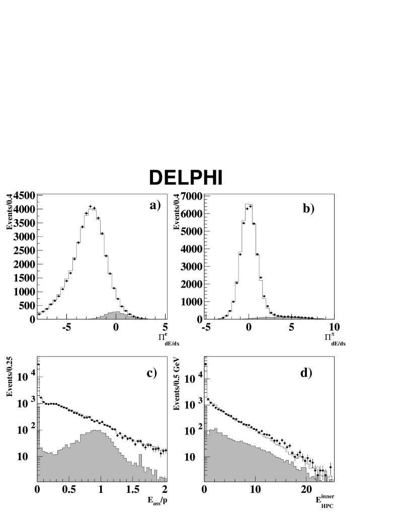
Figure 2: Distributions for hadron test samples in $\tau$-decays of electron-hadron separation variables: a) the variable $\Pi_{dE/dx}^{\rm e}$ ; b) the variable $\Pi_{dE/dx}^{\pi}$ ; c) the variable $\frac{E_{ass}}{P}$ ; d) the energy deposited in the innermost four layers of the HPC. Data are shown as dots and simulation by a solid line. The shaded region represents the simulated background including other $\tau$-decays.

where ${dE/dx}_{meas}$ is the measured value, ${dE/dx}_{exp}(j)$ is the expected momentum dependent value for a hypothesis $j$ and $\sigma(dE/dx)$ is the resolution of the measurement. It was required that there be at least 38 anode sense wires used in the measurement. The $dE/dx$ was calibrated as a function of particle velocity, polar and azimuthal angle. The distributions in simulation were tuned to agree with test samples of real data. The relative precision obtained was  6.2%. Fig. 1 shows the distribution of $\Pi_{dE/dx}^{\mathrm{e}}$ and of $\Pi_{dE/dx}^{\pi}$ in an electron test sample selected using calorimetric cuts. Fig. 2 shows the same distributions for a hadron test sample selected from $\tau$-decays.

4.1.3 Electromagnetic calorimetry

The calibration of the HPC for the energy range from 0.5 GeV to 46 GeV used test samples of electrons in Compton events, both radiative and non-radiative Bhabha events, and electrons tagged by the TPC $dE/dx$ measurement. Since no difference was found in the response for electrons or photons, $\gamma$ samples were also used for the calibration. This will be described in section 4.2.4.

For electrons, the associated energy deposited in the HPC (in GeV), $E_{ass}$, should be equal to the measured value of the momentum (in GeV/c), within experimental errors. For hadrons the energy should be lower than the measured momentum as hadrons typically traverse the HPC leaving only a small fraction of their energy. Muons deposit only a small amount of energy in the HPC.

The ratio of the energy deposition in the HPC to the reconstructed momentum, $p$, has a peak at unity for electrons and a distribution rising towards zero for hadrons. This is shown in Fig. 1 for samples of electrons and Fig. 2 for samples of hadrons. It was also observed [15] that the energy deposition for hadronic showers starting before or inside the HPC had to be downscaled by about 10% in the simulation to get good agreement with data. This is due to an underestimate of the nuclear interaction length of the material in some of the subdetectors.

Electron rejection with high hadron selection efficiency was performed using the associated energy deposition in only the first four layers of the HPC (corresponding to 6$X_{0}$ for perpendicular incidence) in which electrons deposited a significant amount of energy, while hadrons had a small interaction probability. This is shown in Figs. 1 and  2 for electron and hadron test samples from $\tau$-decays.

4.1.4 Hadron calorimetry and muon identification

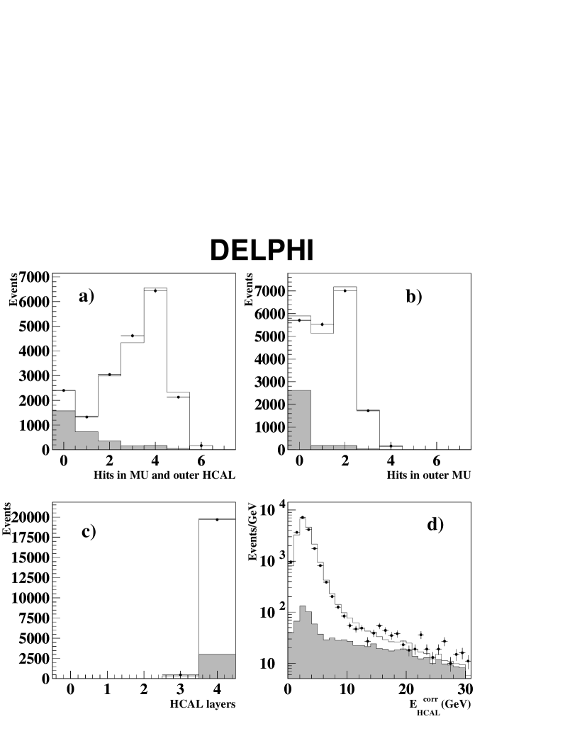
Figure 3: Muon-identification variables for muon test samples in $\tau$-decays: a) number of muon chamber hits including the outer HCAL layer; b) number of muon chamber hits in the outer muon chambers; c) number of layers in the HCAL; d) corrected deposited energy in the HCAL. Data are shown as dots and simulation after the corrections described in the text, by a solid line. The shaded area represents the non-muon background.

The signature of a muon passing through the HCAL was that of a minimum-ionising particle, leaving a roughly constant signal corresponding to an energy deposition of approximately 0.5 GeV in each of the four layers, and penetrating through into the muon chambers. Hadrons, on the other hand, typically deposited most or all of their energy late in the HPC, the superconducting coil, or the first layers of the HCAL, rarely penetrating through to the muon chambers. The response of the HCAL to hadrons depended on the energy of the hadron and where in the detector it interacted. Studies of the HCAL response to muons showed good agreement between data and simulation. For hadrons the total energy deposited in the HCAL was simulated well. However the depth profile of the hadronic showers was not simulated well. This is attributed to cut-offs in the modelling of the tails of hadronic showers in the simulation program. These had a negligible effect on the total deposited energy but a significant effect on the depth profile of the shower. This effect was corrected for by artificially adding an extra layer hit in simulated hadronic showers according to the results obtained from a data sample of charged hadrons produced from a tightly-selected sample of $\tau^{-}\rightarrow\rho^{-}\nu_{\tau}$ decays. An additional HCAL layer with a very low energy deposition was added in $(25.5\pm 0.5)$% of hadronic $\tau$ decays. This fraction and uncertainty were obtained from a fit of the simulation shower depth profile to the data test sample. The distribution after this correction is shown in Figs. 3c) and  4c).

A number of different HCAL quantities gave hadron-muon separation, such as the energy deposition in the outermost HCAL layer, or the total energy in the HCAL, $E_{hcal}$. The total associated HCAL energy, shown in Figs. 3d) and  4d), was corrected, as a function of the number of modules and the amount of material crossed by the particle, in such a way that the response for muons became independent of the polar angle.

The muon chambers typically had between two and five layers hit by a penetrating muon (of momentum greater than 2.5 GeV/$c$.) The response to muons was calibrated using dimuon events. The simulation gave the same muon identification efficiency as the data. Most hadrons and their resultant shower did not penetrate through to the muon chambers, especially the external muon chambers which lay completely outside the magnet yoke. However, because of the poor modelling of the tails of hadronic showers in the simulation program, the probability that a hadron of a given momentum would leave a signal in the muon chambers was higher in the data than in the simulation. This was studied using the same data sample of hadrons in tightly-tagged $\tau^{-}\rightarrow\rho^{-}\nu_{\tau}$ events and in three-prong $\tau$-decays with very low muon contamination. Corrections were applied to the simulation for both the inner and outer layers of muon chambers. These were obtained by adding extra muon chamber hits for hadrons penetrating deeply into the HCAL so as to obtain good agreement between data and simulation. The fraction of extra hits was obtained from a fit of the muon chamber hit distribution in simulation to that for the data test sample. Correlations with the corrections made to the number of HCAL layers hit were taken into account. Figs. 3 and  4, show the response of these detectors for muon and hadron test samples.

4.2 Photons and neutral pions

The reconstruction of photons and hence of $\pi^{0}$ mesons was based principally on the HPC. Electromagnetic showers were reconstructed using only the HPC information without any prior knowledge of charged particles reconstructed in the tracking subdetectors and predicted to enter the HPC. Cuts based on the shower profile in the HPC were applied to photon candidates to reduce the rate of fake photons from the interactions of hadrons in the HPC. An algorithm [17, 6] was applied to individual HPC clusters to see if they were compatible with having been produced by a single $\pi^{0}$ decaying to two photons where the showers due to the two photons overlapped significantly. In addition, photons which had converted to ${\rm e}^{+}{\rm e}^{-}$ pairs in the detector material before the start of the HPC were reconstructed using track segments from the tracking subdetectors.

4.2.1 HPC shower reconstruction

The HPC gave up to nine longitudinal energy samples on a shower. In each sample the energy deposition was measured with a granularity of 2 cm in r-$\phi$ and 3.5 mm in z. The shower pattern recognition proceeded as follows. All samplings in all nine layers were projected on to a cylindrical grid of granularity 3.4 mm $\times$ 1.6 mrad in z $\times$ $\phi$. Neighbouring bins were then added together into a coarser grid of granularity $0.5^{\circ}$ by $0.5^{\circ}$ in $\theta$ and $\phi$. A local maximum search was performed and contiguous areas were separated if a significant minimum was found between two local maxima. All bins connected together after this were grouped together into one cluster. A fit was performed to the cluster transverse profiles to estimate the position of the interacting particle, together with the direction vector of the shower within the HPC. After the shower reconstruction, charged-particle tracks reconstructed in the tracking system were extrapolated to the HPC and associated to a cluster if it was compatible with having been produced by that particle. To increase the efficiency for minimum-ionising particles, additional low-energy clusters could be reconstructed along the track extrapolation.

The substructure of each individual HPC cluster with energy greater than 5 GeV was then studied to ascertain if it was compatible with arising from a (typically high energy) neutral pion where the two photons from the decay produced overlapping showers.

The high granularity of the HPC allowed a measurement of the lateral dimensions of a cluster. For a cluster arising from two photons entering the HPC the angular separation of the two photons is about $m_{\pi^{0}}/E_{\pi^{0}}$ for symmetric pair production (the most difficult case). This is about 7 mrad for $E_{\pi^{0}}=20$ GeV, similar to the granularity of the detector. To search for cluster substructure the energy deposition inside a cluster was plotted on the $\phi-\theta$ plane with each depth layer of the cluster weighted, giving the greatest weights to the more central layers, which had the most spatial-separation power. This two-dimensional distribution of weighted charge deposition was then fitted to a dipole function, projected on to the main axis, and two Gaussian distributions fitted to the projected distribution. The invariant mass was then calculated using the estimated energy deposition in each Gaussian and the opening angle calculated from the fit. Some corrections estimated from simulation were made to account for detector binning effects and biases in the fitting procedure. The main background came from photons converting just before the HPC and which were missed by the photon conversion reconstruction algorithm. This could give rise to a fake $\pi^{0}$ signal or a triple peak substructure in the cluster which was not properly handled by the algorithm. Since the magnetic field deflected charged particles only in $\phi$, this problem was mostly confined to clusters with the dipole axis lying within 100 mrad of the line with constant $\theta$ passing through the cluster barycentre. To optimise the $\pi^{0}-\gamma$ separation with a single variable, a neural network was used which had as inputs the estimated $\pi^{0}$ mass, the fraction of energy in the most energetic of the two photons and the angle of the dipole axis in the cluster. The network had a single output neuron and was trained with a sample of isolated photons in simulated $\mu^{+}\mu^{-}\gamma$ final states to give a target output of zero and on tightly tagged $\pi^{0}$ candidates in simulated $\tau^{-}\rightarrow\rho^{-}\nu_{\tau}$ decays to give a target output of unity.

Fig. 5 shows the invariant-mass distribution and neural network output for single-cluster candidate $\pi^{0}$’s selected from a tightly-tagged $\rho$ sample in two energy ranges ($8<E<12$ GeV and $E>12$ GeV). This Figure also shows the same quantities for an isolated-$\gamma$ test sample from $\mu^{+}\mu^{-}\gamma$.

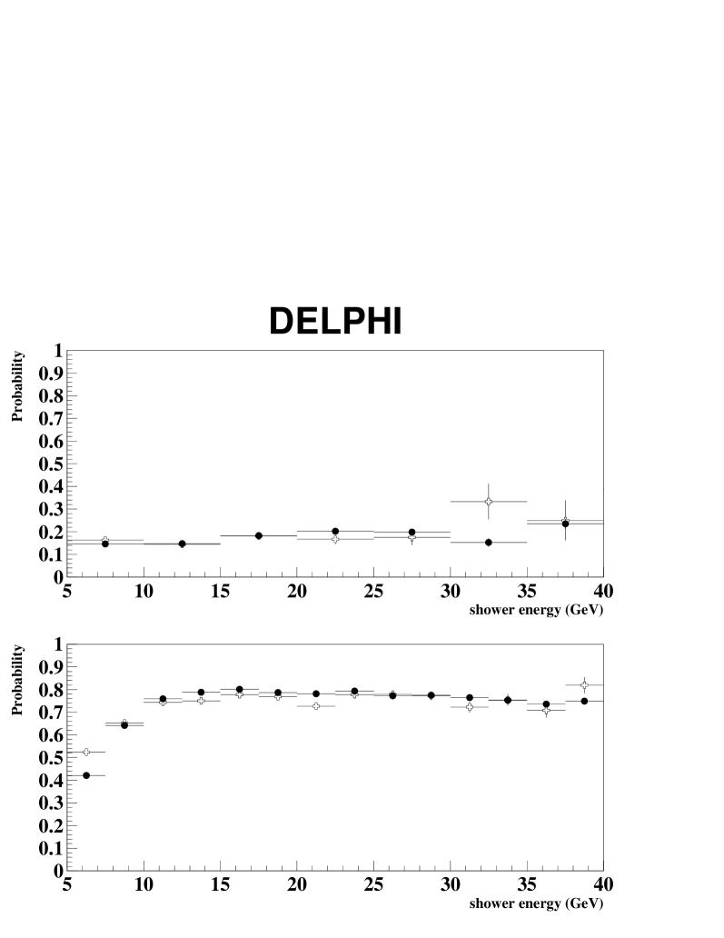
Figure 6: $\pi^{0}$-identification probability in a single shower as a function of the shower energy, obtained from isolated-$\gamma$ samples (a) and $\pi^{0}$ sample in tightly-tagged $\rho$ decays (b). Data are represented by crosses and simulation by filled circles.

The HPC reconstruction was studied using isolated photons in $\mu^{+}\mu^{-}\gamma$ and ${\rm e}^{+}{\rm e}^{-}\gamma$ final states. The probability to identify a single photon as $\pi^{0}$ is shown as a function of the reconstructed HPC cluster energy in Fig. 6a); on average it was $(16.8\pm 0.6)$% on data and $(15.8\pm 0.2)$% in simulation. The efficiency of the algorithm was studied in tightly-tagged $\tau$-decays containing one charged hadron and a single energetic neutral HPC cluster with a combined mass compatible with that of a $\rho$. Simulation studies indicate that such a sample of HPC clusters constituted a $90.5$% pure sample of $\pi^{0}\to\gamma\gamma$ decays. The probability to identify a $\pi^{0}$ is also shown in Fig. 6b) as a function of the reconstructed $\pi^{0}$ energy; on average it was $(69.7\pm 0.5)$% in data and $(69.1\pm 0.1)$% in simulation.

The probability for a photon to be reconstructed as two HPC clusters was found to be a factor $1.15\pm 0.02$ larger in the data, showing an excess of unreconstructed conversions in the material in front of the HPC. The simulation was corrected according to this factor, following the reweighting technique described in [16], and a corresponding systematic uncertainty was assigned.

4.2.2 Converted photons

Photons converting in the material before the HPC fell into two classes, depending on whether the conversion took place before or after the TPC sensitive volume.

About 7% of photons interacted in the material before the TPC gas volume giving an ${\rm e}^{+}{\rm e}^{-}$ pair detected in some of the tracking chambers. These were reconstructed using the tracks observed in the TPC. A detailed study and description of the algorithm and its performance can be found in [16]. In simulation the efficiency to reconstruct a converted photon was found to be $(68.1\pm 0.2)$% in one-prong $\tau$-decays and $(59.8\pm 0.4)$% in three-prong $\tau$-decays. Good agreement between efficiencies in data and simulation was observed, while the simulation program underestimated by about 10% the material before the TPC in terms of radiation lengths. The photons obtained with this kinematic algorithm were in general measured more precisely than those observed in the HPC.

A further 35%/$\sin\theta$ of photons converted in the outer wall of the TPC, the material of the RICH inner wall, liquid radiator, drift tube walls, mirrors, and outer walls, or in the OD. These constituted a problem for the HPC pattern recognition as there was a more limited possibility to reconstruct these conversions with the tracking system as only the OD lay outside this region. Such conversion pairs were split in the DELPHI magnetic field before interacting in the HPC to produce electromagnetic depositions. This created a two-fold problem for the neutral particle pattern recognition: a single photon could produce two showers in the HPC, one from each particle of the ${\rm e}^{+}{\rm e}^{-}$ pair. These were reconstructed as either one or two clusters by the HPC pattern recognition, depending on the spatial separation of the showers. Potentially, both cases could be misidentified as a $\pi^{0}\rightarrow\gamma\gamma$ candidate. Thus the number of reconstructed photons was incorrect. In particular this splitting effect was important for conversions in the outer wall of the TPC or the inner regions of the RICH, far from the first sensitive plane of the HPC.

An algorithm reconstructed these converted photons from the track segments in the OD. The OD consisted of five layers of streamer tubes with a high efficiency for observing a charged particle. An OD track element direction had a resolution in azimuthal angle of about 1 mrad and thus gave an unambiguous determination of the sign of the charge of a particle up to the beam momentum, if this particle originated at radii smaller than 150 cm. If there were two such track elements of different sign of charge in the OD, unassociated to reconstructed charged particles in the TPC, an algorithm which assumed that both track elements were produced by an ${\rm e}^{+}{\rm e}^{-}$ pair from a common conversion point was run. If this common conversion point was compatible with the material structure in the TPC and the RICH and the OD track elements were compatible in polar angle, then this was regarded as a photon. If there were HPC clusters behind the OD track elements these clusters had to have energies which were compatible with the estimated e⁺ and e^- energies derived from the algorithm, in which case the clusters were ignored for further analysis. This algorithm was typically about 25% efficient. Studies of efficiency using radiative dimuon and dielectron events, showed the ratio of post-TPC conversion reconstruction efficiency in data compared with simulation was $0.95\pm 0.07$, consistent with unity.

4.2.3 Hadronic shower rejection

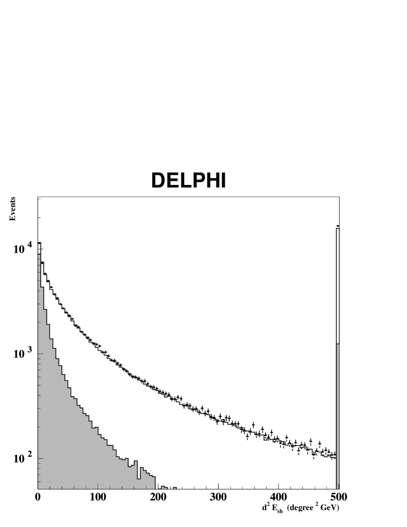
Figure 8: Distributions of the quantity $d^{2}_{sh-ch}E_{sh}$ used for rejection of hadronic showers in the HPC for the inclusive $\tau$ sample of photons with all identification requirements applied except the cut on this variable. Data are shown as dots and simulation by a solid line. The shaded area shows the contribution from showers induced by charged hadrons. The last bin shows the overflows.

The granularity of the HPC was used to remove many clusters of a non-electromagnetic origin, such as hadronic showers occurring in the HPC or before (in the RICH or OD). These have different profiles in the detector due to the difference between the nuclear interaction length and radiation length of lead, and the difference in the sampling efficiency for the different processes through which their energy is absorbed. To be accepted as a photon shower a cluster had to have both longitudinal and transverse profiles consistent with those expected for an electromagnetic deposition [6]. This requirement rejected most showers from hadronic interactions. In Fig. 7, the distributions of two quantities related to the cluster profile in the HPC, namely the number of layers and the fraction of energy deposited in the first four layers, are shown for candidate photons selected after this pattern recognition. A good agreement between data and simulation is observed. Because of the high momentum of the charged hadron and the proximity to the $\pi^{0}$’s, features typical of $\tau$-decays, additional criteria were applied to reduce further the contamination from hadronic showers. Many hadronic showers were rejected by accepting only those clusters for which the reconstructed energy, $E_{sh}$, was greater than 500 MeV. The quantity $d^{2}_{sh-ch}E_{sh}$ had to be greater than $10\deg^{2}$GeV, where $d_{sh-ch}$ was the opening angle between the cluster and the track extrapolation at the HPC inner surface. This variable tends to be strongly peaked at low values for fake showers originating from splits of hadronic showers in the HPC, because they were typically of low energy and close to the track entry point in the HPC, in contrast to those originating from a photon produced in a $\tau$ decay. The distribution of this quantity is shown in Fig. 8, showing good agreement between data and simulation. No hadronic rejection criteria were applied to HPC clusters which were identified as candidate $\pi^{0}$ mesons with the single-shower $\pi^{0}$ algorithm, as such clusters benefited from a low background.

In Fig. 9 the energy spectra for selected HPC clusters are shown for the maximum- and minimum-energy photon in a $\tau$ decay hemisphere, for different numbers of reconstructed clusters in that hemisphere. The agreement between data and simulation is good in all cases for both the low-energy region and the high-energy region.

The full photon reconstruction efficiency was studied in two steps. First, electron samples where the track had left a signal in the OD, with a small probability of having interacted before reaching the HPC, were used to estimate the shower reconstruction efficiency. Isolated $\gamma$ samples from radiative $ee$ and $\mu\mu$ were used to check the shower profile cuts. The efficiency in the data was found to be $(0.3\pm 0.2)$% less than in the simulation.

The production of fake photons from hadronic interactions was estimated from the data and simulation agreement in the distribution shown in Fig. 8, for small values of the variable, where the fake photons rate is comparable to that of the real photons. The simulation was found to reproduce correctly the data to a relative $3$%.

4.2.4 Energy scale

In addition to the previously measured electron samples, the HPC energy scale was studied using isolated photons in $\mu^{+}\mu^{-}\gamma$ and ${\rm e}^{+}{\rm e}^{-}\gamma$ final states and $e\gamma$ compton scattering events. In these three cases the direction is well defined and the particle energy can be inferred with a very good precision using kinematic constraints, independently from the energy measurement in the calorimeter. This allowed the HPC energy response to be calibrated as a function of energy. A precision of 0.5% or better was obtained on the energy scale throughout the entire energy spectrum. The measured energy resolution was $\sigma(E)/E=0.31\times E^{-0.44}\oplus 0.027$.

4.2.5 Spatial resolution

The efficiency to reconstruct electromagnetic showers close to charged hadron tracks and showers in the HPC is important in $\tau$-decays where the $\tau$-decay products are tightly collimated. To illustrate this, Fig. 10 shows the minimum angular distance between different types of HPC clusters: neutral clusters fulfilling the photon requirements, those failing them and those associated to a charged particle. The good agreement of data and simulation in the region of very small opening angles demonstrates that all these effects are simulated correctly.

4.2.6 Neutral pions

Fig 11 shows, as a function of $\pi^{0}$ energy, the probability, in a simulated $\rho$ sample from $\tau$-decays, for a $\pi^{0}$ to produce a given number of HPC or converted photons. The efficiency to observe one or more photons from one $\pi^{0}$ in the angular acceptance of the HPC is high, dropping below 85% only in the region below 3 GeV.

Reconstructed neutral pions fell into four different categories. The first class (I) consisted of $\pi^{0}$ candidates identified with the single cluster algorithm described in Section 4.2.1. The second class (II) contained $\pi^{0}$ candidates reconstructed from pairs of photons identified as separate HPC clusters, while the third class (III) contained $\pi^{0}$ candidates reconstructed from pairs of photons, of which at least one was a reconstructed converted photon. The $\gamma\gamma$ invariant-mass distributions for classes II and III of candidate $\pi^{0}$ are shown in Fig. 12. Class I dominated for the high-energy region, the class II contributed significantly in the region below 10 GeV, while the class III had a rather flat energy dependence.

The fourth class (IV) recuperated photons in single-prong $\tau$-decays where a photon was accidentally associated to a charged-hadron track. For $\tau$-decay hemispheres where the HPC cluster associated to the track satisfied the photon-candidate requirements in all other respects, and where there was an additional photon candidate, the HPC cluster was disassociated from the track, provided that the invariant mass $m_{\gamma\gamma}$ of the $\gamma\gamma$ system was greater than 70 MeV/$c^{2}$. Simulation studies indicated that such decays were predominantly due to the $\pi^{\pm}\pi^{0}\nu_{\tau}$ decay mode. The $m_{\gamma\gamma}$ distribution for this class of $\pi^{0}$ is also shown in Fig. 12, before the mass cut.

Fig 13 shows the total identification efficiency as well as the probability to classify a $\pi^{0}$ in each of the four categories discussed above as a function of the $\pi^{0}$ energy for simulated $\rho$ decays.

It is important to note that many of the high energy showers, despite not being resolved as $\pi^{0}$, are nevertheless most likely to come from a merged $\pi^{0}$. This accounted for in the analyses in such a way that, depending on other variables, a single shower not identified as $\pi^{0}$ by any of the above criteria could be considered as a $\pi^{0}$.

5 Selection of ${\rm e}^{+}{\rm e}^{-}\rightarrow\tau^{+}\tau^{-}$ events

The selection of the ${\rm e}^{+}{\rm e}^{-}\rightarrow Z\rightarrow\tau^{+}\tau^{-}$ event sample is identical to that used in [16]. Only a summary is given here.

In the ${\rm e}^{+}{\rm e}^{-}\rightarrow Z\rightarrow\tau^{+}\tau^{-}$ reaction at $\sqrt{s}=M_{Z}$ , neglecting radiative effects, the $\tau^{+}$ and $\tau^{-}$ are produced back-to-back. The $\tau$’s each decay to one, three or five charged and one or more neutral particles in a tightly collimated jet. Thus a $\tau^{+}\tau^{-}$ event is characterised by two low-multiplicity jets which appear back-to-back in the laboratory frame. Because each $\tau$ emits at least one undetectable neutrino or anti-neutrino, the full event energy is not observed in the detector.

Background events have various signatures which enable them to be separated from the signal. For the ${\rm e}^{+}{\rm e}^{-}\rightarrow{\rm q}\bar{\rm q}$ channel, the typical charged-particle multiplicity is about 20, and quark fragmentation produces less-collimated jets. The ${\rm e}^{+}{\rm e}^{-}\rightarrow{\rm e}^{+}{\rm e}^{-}$ and ${\rm e}^{+}{\rm e}^{-}\rightarrow\mu^{+}\mu^{-}$ processes give a 1 versus 1 charged-particle topology, no neutral electromagnetic showers, and contain the full event energy measured in the detector due to the absence of final-state neutrinos. Two-photon events tend to have low energy visible in the detector due to the loss of the ${\rm e}^{+}{\rm e}^{-}$ pair in the beam-pipe. Cosmic rays can be removed using cuts on the distance of closest approach to the interaction region.

The data were passed through the photon conversion algorithm outlined in Section 4.2 to give an improved estimate of the numbers of charged and neutral particles in an event. To ensure that the $\tau$ products lay in the acceptance of the relevant subdetectors it was demanded that the thrust axis of the event lie within the polar-angle region defined by $|\cos\theta|<0.732$ and that there be at least one charged particle in the polar-angle region defined by $|\cos\theta|>0.035$. The event was split into two hemispheres, each associated to a candidate $\tau$ decay, by a plane perpendicular to the thrust axis and passing through the centre of the interaction region. It was required that there be at least one charged particle in each hemisphere.

Hadronic decays of the Z were suppressed by requiring that there be a maximum of eight charged particles in an event. Background from four-fermion events was reduced, together with a further suppression of Z hadronic decays, by requiring that the event isolation angle be greater than $160^{\circ}$. The isolation angle was defined as the minimum angle between any pair of charged particles which were associated to opposite $\tau$-decay hemispheres. Backgrounds from $\mu^{+}\mu^{-}$ and ${\rm e}^{+}{\rm e}^{-}$ final states and cosmic rays were reduced by requiring that the isolation angle be less than $179.5^{\circ}$ for events with only two charged particles.

The $\mu^{+}\mu^{-}$ and ${\rm e}^{+}{\rm e}^{-}$ contamination was reduced further by requiring that both $p_{rad}=\sqrt{\frac{|\vec{p}_{1}|^{2}}{{p_{1}^{\prime}}^{2}}+\frac{|\vec{p}_{2}|^{2}}{{p_{2}^{\prime}}^{2}}}$ and $E_{rad}=\sqrt{\frac{E_{1}^{2}}{{E_{1}^{\prime}}^{2}}+\frac{E_{2}^{2}}{{E_{2}^{\prime}}^{2}}}$ be less than unity. The variables $\vec{p}_{1}$ and $\vec{p}_{2}$ are the momenta of the highest-momentum charged particles in hemispheres 1 and 2 respectively. The quantity $p_{1}^{\prime}$ was obtained from the formula $p_{1}^{\prime}=\sqrt{s}\sin\theta_{2}/(\sin\theta_{1}+\sin\theta_{2}+|\sin(\theta_{1}+\theta_{2})|)$, and $p_{2}^{\prime}$ by analogy with the indices 1 and 2 interchanged. The angles $\theta_{1}$ and $\theta_{2}$ are the polar angles of the highest-momentum charged particle in hemispheres 1 and 2 respectively. The variables $E_{1}$ and $E_{2}$ are the total electromagnetic energies deposited in cones of half-angle $30^{\circ}$ about the momentum vectors $\vec{p}_{1}$ and $\vec{p}_{2}$ respectively, while $E_{j}^{\prime}=cp_{j}^{\prime}$, for $j=1,2$. Much of the remaining background from the dileptonic channels came from events containing hard radiation lying far from the beam. These events should lie in a plane. Where two charged particles and a photon were visible in the detector, such events were removed when the sum of the angles between the three particles was greater than $359.8^{\circ}$.

Further reduction of the four-fermion contamination was achieved by requiring that there be a minimum visible energy of $0.09\times\sqrt{s}$ in the event. Energy deposits recorded by the luminometers (the SAT or STIC) at angles of less than $12^{\circ}$ from the beam axis were excluded from this quantity. For events with only two charged particles, the additional condition that the vectorial sum of the components of the charged-particle momenta transverse to the beam be greater than 0.4 GeV/$c$ was applied. Two-photon events typically have very low values of total transverse momentum compared with $\tau^{+}\tau^{-}$ events.

Most cosmic rays were removed by the cut on isolation angle. Further rejection was carried out by requiring that at least one charged particle in the event have a perigee with respect to the interaction region of less than 0.3 cm in the r-$\phi$ plane and that both event hemispheres have a charged particle whose perigee point lay within 4.5 cm of the interaction region in z and 1.5 cm in r-$\phi$.

In a final step, a neural network was used to reduce the background from hadronic Z decays [16].

The efficiency of the selection was estimated from simulation to be $(51.74\pm 0.04)$%. Within the angular acceptance it was about 85%. A total of 80337 candidate ${\rm e}^{+}{\rm e}^{-}\rightarrow\tau^{+}\tau^{-}$ events was selected.

The background levels were estimated from the data themselves by fitting a normalisation factor to the background contribution in variables sensitive to a particular background, assuming that the shape of the background was that given by simulation, and where possible using particle identification to isolate particular backgrounds. The total background was estimated to be $(1.51\pm 0.10)$%. The different contributions are shown in Table. 1. The backgrounds from $\mu^{+}\mu^{-}\mu^{+}\mu^{-}$, $\mu^{+}\mu^{-}\tau^{+}\tau^{-}$ and $\tau^{+}\tau^{-}\tau^{+}\tau^{-}$ final states were negligible.

Source of	$\tau^{+}\tau^{-}$
Background	selection
$\mu^{+}\mu^{-}$	0.11$\pm$	0.01
${\rm e}^{+}{\rm e}^{-}$	0.40$\pm$	0.07
${\rm q}\bar{\rm q}$	0.29$\pm$	0.01
${\rm e}^{+}{\rm e}^{-}{\rm e}^{+}{\rm e}^{-}$	0.27$\pm$	0.03
${\rm e}^{+}{\rm e}^{-}\mu^{+}\mu^{-}$	0.10$\pm$	0.01
${\rm e}^{+}{\rm e}^{-}\tau^{+}\tau^{-}$	0.27$\pm$	0.03
${\rm e}^{+}{\rm e}^{-}{\rm q}\bar{\rm q}$	0.02$\pm$	0.01
cosmic rays	0.05$\pm$	0.01

Table 1: Selected non-$\tau^{+}\tau^{-}$ backgrounds, in percent, in the total sample.

6 Charged-particle multiplicity selection

The selection of $\tau$-decays according to the charged-particle multiplicity was identical to that carried out for the categories 1, 3 and 5 in the DELPHI measurement [16] of the $\tau$ topological branching ratios and only a brief description is given here. In the following a “good” track is defined as a track with associated hits in either the TPC or OD. The VD-ID tracks include not only tracks reconstructed in the VD and ID without TPC or OD but also particles reconstructed from the decay products of nuclear interactions in the detector material.

A one-prong $\tau$-decay was defined as a $\tau$-decay hemisphere satisfying any of the following criteria:

• only one good track with at least one associated VD hit, and no other tracks with associated VD hits;

• only one good track, without VD or ID hits, and one VD-ID track;

• no good tracks, and only one VD-ID track.

three-prong $\tau$-decays were isolated by demanding $\tau$-decay hemispheres satisfying at least one of the following sets of criteria:

• three, four or five good tracks, of which either two or three had associated VD hits;

• two good tracks with associated VD hits, plus one VD-ID track;

• one good track with associated VD hits, plus one or two VD-ID tracks pointing within $3^{\circ}$ in azimuth to a TPC sector boundary.

Candidate five-prong $\tau$-decays were selected if they satisfied at least one of the following topological criteria:

• five good tracks of which at least four had two or more associated VD hits;

• four good tracks with associated VD hits, and one other VD-ID track.

Additional criteria were applied in the selection of five-prong $\tau$-decays due to the large potential background from hadronic Z decays and misreconstructed three-prong $\tau$-decays. The background originating from $3h^{\pm}\geq 1\pi^{0}\nu_{\tau}$ final states with a Dalitz decay was expected to occur at a similar level to the signal. Electron-rejection criteria based on $E_{ass}/P$ and $dE/dx$ described in Section 4.1 reduced this background by about 70%, and it was further suppressed by requiring that all good tracks had a reconstructed momentum greater than 1 GeV/$c$. To reject Z$\to{\rm q}\bar{\rm q}$ events it was required that the total momentum of the the five-prong system be greater than 20 GeV/$c$. Only good tracks were included in the calculation of this quantity.

Table 2 contains the efficiencies of these selection requirements for the different exclusive $\tau$-decay modes and the charged particle multiplicity selections, as obtained from simulation and after corrections for observed discrepancies between data and simulation in the rate and reconstruction efficiency of material reinteractions.

true $\tau$	$\tau^{+}\tau^{-}$		Charged Multiplicity Classification
decay mode	selection		1		3		5
$\rm e^{-}\nu_{\tau}\bar{\nu}_{\mathrm{e}}$	50.60$\pm$	0.07	99.95$\pm$	0.00	0.00$\pm$	0.00	0.00$\pm$	0.00
$\mu^{-}\nu_{\tau}\bar{\nu}_{\mu}$	53.31$\pm$	0.07	99.96$\pm$	0.00	0.00$\pm$	0.00	0.00$\pm$	0.00
$\pi^{-}\nu_{\tau}$	49.69$\pm$	0.09	99.88$\pm$	0.01	0.04$\pm$	0.01	0.00$\pm$	0.00
$K^{-}\nu_{\tau}$	49.43$\pm$	0.36	99.90$\pm$	0.03	0.02$\pm$	0.02	0.00$\pm$	0.00
$\pi^{-}K^{0}_{\!\mathrm{L}}\nu_{\tau}$	53.10$\pm$	0.48	99.79$\pm$	0.06	0.07$\pm$	0.03	0.00$\pm$	0.00
$K^{-}K^{0}_{\!\mathrm{L}}\nu_{\tau}$	54.60$\pm$	0.87	99.78$\pm$	0.11	0.11$\pm$	0.08	0.00$\pm$	0.00
$\pi^{-}K^{0}_{\!\mathrm{S}}\nu_{\tau}$	52.17$\pm$	0.48	94.48$\pm$	0.30	4.30$\pm$	0.27	0.00$\pm$	0.00
$K^{-}K^{0}_{\!\mathrm{S}}\nu_{\tau}$	52.38$\pm$	0.86	94.50$\pm$	0.54	4.42$\pm$	0.49	0.00$\pm$	0.00
$\pi^{-}K^{0}_{\!\mathrm{L}}K^{0}\nu_{\tau}$	52.82$\pm$	1.04	95.12$\pm$	0.62	3.72$\pm$	0.54	0.00$\pm$	0.00
$\pi^{-}2K^{0}_{\!\mathrm{S}}\nu_{\tau}$	46.34$\pm$	1.80	86.72$\pm$	1.80	10.45$\pm$	1.63	0.00$\pm$	0.00
$\pi^{-}\pi^{0}\nu_{\tau}$	51.77$\pm$	0.06	97.87$\pm$	0.03	0.60$\pm$	0.01	0.00$\pm$	0.00
$K^{-}\pi^{0}\nu_{\tau}$	51.40$\pm$	0.47	97.66$\pm$	0.20	0.85$\pm$	0.12	0.00$\pm$	0.00
$\pi^{-}\pi^{0}K^{0}_{\!\mathrm{L}}\nu_{\tau}$	51.85$\pm$	0.73	97.32$\pm$	0.33	0.78$\pm$	0.18	0.00$\pm$	0.00
$K^{-}\pi^{0}K^{0}_{\!\mathrm{L}}\nu_{\tau}$	52.66$\pm$	1.24	96.71$\pm$	0.61	0.94$\pm$	0.33	0.00$\pm$	0.00
$\pi^{-}\pi^{0}K^{0}_{\!\mathrm{S}}\nu_{\tau}$	50.78$\pm$	0.73	92.64$\pm$	0.54	4.65$\pm$	0.43	0.00$\pm$	0.00
$K^{-}\pi^{0}K^{0}_{\!\mathrm{S}}\nu_{\tau}$	51.32$\pm$	1.32	92.56$\pm$	0.97	5.01$\pm$	0.80	0.00$\pm$	0.00
$\pi^{-}2\pi^{0}\nu_{\tau}$	51.07$\pm$	0.11	95.88$\pm$	0.06	1.25$\pm$	0.03	0.00$\pm$	0.00
$K^{-}2\pi^{0}\nu_{\tau}$	50.42$\pm$	1.12	94.65$\pm$	0.71	2.28$\pm$	0.47	0.00$\pm$	0.00
$\pi^{-}3\pi^{0}\nu_{\tau}$	48.89$\pm$	0.25	94.36$\pm$	0.16	1.68$\pm$	0.09	0.00$\pm$	0.00
$2\pi^{-}\pi^{+}\nu_{\tau}$	54.71$\pm$	0.11	0.90$\pm$	0.03	90.26$\pm$	0.09	0.01$\pm$	0.00
$K^{-}\pi^{-}\pi^{+}\nu_{\tau}$	54.64$\pm$	0.56	1.03$\pm$	0.15	90.35$\pm$	0.45	0.00$\pm$	0.00
$K^{-}K^{+}\pi^{+}\nu_{\tau}$	53.87$\pm$	0.90	2.08$\pm$	0.35	87.23$\pm$	0.82	0.00$\pm$	0.00
$2\pi^{-}\pi^{+}\pi^{0}\nu_{\tau}$	53.88$\pm$	0.13	1.26$\pm$	0.04	86.39$\pm$	0.12	0.10$\pm$	0.01
$3\pi^{\pm}2\pi^{0}\nu_{\tau}$	53.14$\pm$	0.46	1.37$\pm$	0.15	83.64$\pm$	0.46	0.22$\pm$	0.06
$3\pi^{\pm}3\pi^{0}\nu_{\tau}$	52.13$\pm$	1.06	1.46$\pm$	0.35	78.73$\pm$	1.20	0.17$\pm$	0.12
$3\pi^{-}2\pi^{+}\nu_{\tau}$	49.63$\pm$	1.19	0.11$\pm$	0.11	12.63$\pm$	1.13	57.52$\pm$	1.67
$3\pi^{-}2\pi^{+}\pi^{0}\nu_{\tau}$	48.91$\pm$	2.23	0.00$\pm$	0.00	15.04$\pm$	2.28	52.85$\pm$	3.18

Table 2: Estimates of the $\tau^{+}\tau^{-}$ selection- and topology-classification efficiencies, in percent, for different exclusive decay modes, as obtained from simulation. The efficiencies are corrected for observed discrepancies between data and simulation in the rate and reconstruction efficiency of material reinteractions. The quoted uncertainties are from the simulation statistics only. When no events are classified in a given class the Poissonian upper bound is taken as error. Numbers smaller than 0.005% are represented in the table as 0.00.

In this analysis the quality of reconstruction of the charged particle tracks, especially their momentum and precision of the extrapolation to the calorimeters, was important for identification pourposes. Thus an additional requirement was made that candidate one-prong $\tau$-decays should contain a “good” track. This rejected candidate $\tau$-decays reconstructed with only a VD-ID track or with the inelastic nuclear interaction reconstruction algorithm. These have been extensively studied in [16] and the necessary corrections for any data/simulation discrepancies were applied, and the related uncertainties estimated.

The data sample of $\tau$-decays contained 134421 candidate one-prong decays, 23847 candidate three-prong decays and 112 candidate five-prong decays.

7 Selection of (semi-)exclusive $\tau$-decay modes

Analyses using sequential cuts and neural networks identified the different decay modes. In both cases, the different channel selections were applied simultaneously to take into account statistical and systematic correlations.

The following decay modes were selected using sequential cuts (where $h=\pi$ or $K$): $h^{-}\nu_{\tau}$, $h^{-}\pi^{0}\nu_{\tau}$, $h^{-}\geq\!2\pi^{0}\nu_{\tau}$, $2h^{-}h^{+}\nu_{\tau}$, $2h^{-}h^{+}\geq 1\pi^{0}\nu_{\tau}$, $3h^{-}2h^{+}\nu_{\tau}$ and $3h^{-}2h^{+}\pi^{0}\nu_{\tau}$. The neural-network analysis was only performed for the one- and three-prong decays and included the following additional modes: $h^{-}2\pi^{0}\nu_{\tau}$, $h^{-}\geq\!3\pi^{0}\nu_{\tau}$, $2h^{-}h^{+}\pi^{0}\nu_{\tau}$ and $2h^{-}h^{+}\geq 2\pi^{0}\nu_{\tau}$. It also included a measurement of the electronic and muonic branching ratios. Although no dedicated selection is present, we also quote the branching ratio for the inclusive channel $h^{-}\geq\!1\pi^{0}\nu_{\tau}$, obtained by adding all the modes with at least one $\pi^{0}$.

In this analysis there is no explicit $K^{0}$ rejection or identification and the selection efficiencies were, to first order, independent of the presence of neutral kaons. These decays were therefore included in the equivalent class without $K^{0}$. This was done regardless of the $K^{0}$ decay (even for the decay mode $\tau^{-}\rightarrow h^{-}K^{0}\nu_{\tau}\to h^{-}\pi^{0}\pi^{0}\nu_{\tau}$) or of their interaction in the detector. For other mesons, the decays were classified according to the number of charged pions, charged kaons and neutral pions except for the decay modes containing $\eta$ with subsequent decay to $\gamma\gamma$ or $\pi^{+}\pi^{-}\gamma$ and $\omega$ with subsequent decay to $\pi^{0}\gamma$. These decay modes are difficult to isolate from the decay modes measured in this analysis, but are treated as background. Their total branching ratio was [18] $(0.289\pm 0.027)$%, $(0.266\pm 0.027)$% in one-prong decays and $(0.023\pm 0.003)$% for three-prongs. The branching ratios have been corrected for these backgrounds.

7.1 Sequential-Cuts Analysis

The various hadronic decay modes were selected with the cuts described below. The selection efficiencies and cross-talk between channels are given in Table 3 for the one- and three-prong modes, together with the backgrounds from non-$\tau^{+}\tau^{-}$ sources. Table 4 contains the analogous information for the five-prong decay modes. The analysis for leptonic decays is described in [15].

true $\tau$	Sequential cuts decay classification
decay mode	$h^{-}\nu_{\tau}$		$h^{-}\pi^{0}\nu_{\tau}$		$h^{-}\geq 2\pi^{0}\nu_{\tau}$		$3h^{\pm}\nu_{\tau}$		$3h^{\pm}\!\!\geq\!\!1\pi^{0}\nu_{\tau}$
$\rm e^{-}\nu_{\tau}\bar{\nu}_{\mathrm{e}}$	0.11$\pm$	0.01	0.89$\pm$	0.02	0.03$\pm$	0.00	0.00$\pm$	0.00	0.00$\pm$	0.00
$\mu^{-}\nu_{\tau}\bar{\nu}_{\mu}$	1.62$\pm$	0.03	0.22$\pm$	0.01	0.00$\pm$	0.00	0.00$\pm$	0.00	0.00$\pm$	0.00
$\pi^{-}\nu_{\tau}$	49.69$\pm$	0.13	1.44$\pm$	0.03	0.20$\pm$	0.01	0.03$\pm$	0.01	0.01$\pm$	0.00
$K^{-}\nu_{\tau}$	50.82$\pm$	0.53	1.18$\pm$	0.12	0.21$\pm$	0.05	0.05$\pm$	0.02	0.01$\pm$	0.01
$\pi^{-}K^{0}_{\!\mathrm{L}}\nu_{\tau}$	28.45$\pm$	0.61	7.86$\pm$	0.37	0.70$\pm$	0.11	0.05$\pm$	0.03	0.02$\pm$	0.02
$K^{-}K^{0}_{\!\mathrm{L}}\nu_{\tau}$	29.73$\pm$	1.40	7.20$\pm$	0.79	0.48$\pm$	0.21	0.00$\pm$	0.09	0.13$\pm$	0.11
$\pi^{-}K^{0}_{\!\mathrm{S}}\nu_{\tau}$	5.30$\pm$	0.31	13.92$\pm$	0.48	2.23$\pm$	0.20	3.37$\pm$	0.25	0.51$\pm$	0.10
$K^{-}K^{0}_{\!\mathrm{S}}\nu_{\tau}$	6.88$\pm$	0.78	11.77$\pm$	0.99	3.06$\pm$	0.53	3.48$\pm$	0.56	0.55$\pm$	0.23
$\pi^{-}K^{0}_{\!\mathrm{L}}K^{0}\nu_{\tau}$	7.64$\pm$	0.79	13.23$\pm$	1.00	3.96$\pm$	0.58	0.09$\pm$	0.06	1.05$\pm$	0.21
$\pi^{-}2K^{0}_{\!\mathrm{S}}\nu_{\tau}$	0.43$\pm$	0.34	14.33$\pm$	1.81	9.40$\pm$	1.51	5.89$\pm$	1.22	5.22$\pm$	1.15
$\pi^{-}\pi^{0}\nu_{\tau}$	1.37$\pm$	0.02	44.08$\pm$	0.09	3.03$\pm$	0.03	0.21$\pm$	0.01	0.36$\pm$	0.01
$K^{-}\pi^{0}\nu_{\tau}$	1.22$\pm$	0.13	30.79$\pm$	0.56	2.33$\pm$	0.18	0.25$\pm$	0.06	0.40$\pm$	0.08
$\pi^{-}\pi^{0}K^{0}_{\!\mathrm{L}}\nu_{\tau}$	0.89$\pm$	0.19	39.13$\pm$	0.98	8.23$\pm$	0.55	0.09$\pm$	0.06	1.05$\pm$	0.21
$K^{-}\pi^{0}K^{0}_{\!\mathrm{L}}\nu_{\tau}$	0.43$\pm$	0.22	13.45$\pm$	1.13	4.70$\pm$	0.70	0.34$\pm$	0.19	1.19$\pm$	0.36
$\pi^{-}\pi^{0}K^{0}_{\!\mathrm{S}}\nu_{\tau}$	0.08$\pm$	0.06	26.10$\pm$	0.90	16.08$\pm$	0.75	0.45$\pm$	0.14	3.96$\pm$	0.40
$K^{-}\pi^{0}K^{0}_{\!\mathrm{S}}\nu_{\tau}$	0.22$\pm$	0.17	15.07$\pm$	1.29	8.45$\pm$	1.00	1.26$\pm$	0.40	3.43$\pm$	0.65
$\pi^{-}2\pi^{0}\nu_{\tau}$	0.05$\pm$	0.01	19.30$\pm$	0.10	25.50$\pm$	0.12	0.12$\pm$	0.01	1.81$\pm$	0.04
$K^{-}2\pi^{0}\nu_{\tau}$	0.00$\pm$	0.10	17.26$\pm$	1.18	23.08$\pm$	1.31	0.00$\pm$	0.10	2.20$\pm$	0.46
$\pi^{-}3\pi^{0}\nu_{\tau}$	0.02$\pm$	0.01	10.65$\pm$	0.25	41.23$\pm$	0.40	0.05$\pm$	0.02	2.16$\pm$	0.12
$2\pi^{-}\pi^{+}\nu_{\tau}$	0.02$\pm$	0.00	1.82$\pm$	0.03	0.13$\pm$	0.01	71.82$\pm$	0.10	6.72$\pm$	0.05
$K^{-}\pi^{-}\pi^{+}\nu_{\tau}$	0.00$\pm$	0.02	1.55$\pm$	0.19	0.09$\pm$	0.05	73.05$\pm$	0.68	7.31$\pm$	0.40
$K^{-}K^{+}\pi^{+}\nu_{\tau}$	0.00$\pm$	0.02	1.58$\pm$	0.19	0.05$\pm$	0.05	73.58$\pm$	0.81	7.65$\pm$	0.49
$2\pi^{-}\pi^{+}\pi^{0}\nu_{\tau}$	0.00$\pm$	0.00	1.14$\pm$	0.04	0.90$\pm$	0.04	18.71$\pm$	0.16	45.79$\pm$	0.21
$3\pi^{\pm}2\pi^{0}\nu_{\tau}$	0.00$\pm$	0.01	0.38$\pm$	0.07	1.98$\pm$	0.16	6.26$\pm$	0.28	61.84$\pm$	0.56
$3\pi^{\pm}3\pi^{0}\nu_{\tau}$	0.00$\pm$	0.08	0.08$\pm$	0.08	2.94$\pm$	0.48	2.33$\pm$	0.43	64.63$\pm$	1.37
$3\pi^{-}2\pi^{+}\nu_{\tau}$	0.00$\pm$	0.21	0.16$\pm$	0.21	0.20$\pm$	0.21	13.67$\pm$	1.56	14.40$\pm$	1.59
$3\pi^{-}2\pi^{+}\pi^{0}\nu_{\tau}$	0.00$\pm$	0.83	1.00$\pm$	0.91	0.00$\pm$	0.83	1.89$\pm$	1.24	21.66$\pm$	3.76
Source	Non-$\tau^{+}\tau^{-}$ backgrounds
$\mu^{+}\mu^{-}$	0.02$\pm$	0.01	0.06$\pm$	0.01	0.02$\pm$	0.01	0.00$\pm$	0.00	0.00$\pm$	0.00
${\rm e}^{+}{\rm e}^{-}$	0.05$\pm$	0.02	0.10$\pm$	0.02	0.03$\pm$	0.02	0.00$\pm$	0.00	0.00$\pm$	0.00
${\rm q}\bar{\rm q}$	0.15$\pm$	0.03	0.09$\pm$	0.02	0.17$\pm$	0.04	0.29$\pm$	0.03	1.20$\pm$	0.12
$4f$	0.39$\pm$	0.07	0.31$\pm$	0.04	0.23$\pm$	0.06	0.14$\pm$	0.03	0.11$\pm$	0.05

Table 3: For the sequential-cuts analysis, classification efficiencies, in percent, for different exclusive one- and three-prong decay modes, as obtained from simulation after correction for the data/simulation discrepancies discussed in the text. The bottom part shows the backgrounds in percent in each class from non-$\tau^{+}\tau^{-}$ sources. The quoted uncertainties are from the simulation statistics only. When no events are classified in a given class the Poissonian upper bound is taken as error. Numbers smaller than 0.005% are represented in the table as 0.00.

true $\tau$	Decay classification
decay mode	$5h^{\pm}\nu_{\tau}$		$5h^{\pm}\!\!\geq\!\!1\pi^{0}\nu_{\tau}$
$2\pi^{-}\pi^{+}\nu_{\tau}$	0.00$\pm$	0.00	0.00$\pm$	0.00
$K^{-}\pi^{-}\pi^{+}\nu_{\tau}$	0.00$\pm$	0.02	0.00$\pm$	0.02
$K^{-}K^{+}\pi^{+}\nu_{\tau}$	0.00$\pm$	0.02	0.00$\pm$	0.02
$2\pi^{-}\pi^{+}\pi^{0}\nu_{\tau}$	0.11$\pm$	0.01	0.01$\pm$	0.00
$3\pi^{\pm}2\pi^{0}\nu_{\tau}$	0.10$\pm$	0.04	0.05$\pm$	0.03
$3\pi^{\pm}3\pi^{0}\nu_{\tau}$	0.00$\pm$	0.08	0.17$\pm$	0.12
$3\pi^{-}2\pi^{+}\nu_{\tau}$	55.26$\pm$	2.25	3.63$\pm$	0.85
$3\pi^{-}2\pi^{+}\pi^{0}\nu_{\tau}$	35.60$\pm$	4.37	17.68$\pm$	3.48
Source	Non-$\tau^{+}\tau^{-}$ backgrounds
$\mu^{+}\mu^{-}$	0.00$\pm$	0.00	0.00$\pm$	0.00
${\rm e}^{+}{\rm e}^{-}$	0.00$\pm$	0.00	0.00$\pm$	0.00
${\rm q}\bar{\rm q}$	4.55$\pm$	2.63	0.00$\pm$	0.00
$4f$	0.00$\pm$	0.00	0.00$\pm$	0.00

Table 4: For the sequential cuts analysis, the top part contains estimates of classification efficiencies, in percent, for different exclusive five-prong decay modes, as obtained from simulation after correction for the data/simulation discrepancies discussed in the text. The bottom part shows backgrounds from non-$\tau^{+}\tau^{-}$ sources. The quoted uncertainties are from the simulation statistics only.

7.1.1 One-prong decays

In the selection of $\tau^{-}\rightarrow h^{-}\nu_{\tau}$ decays, the separation of a single hadron from electrons and muons requires the use of most of the components of the DELPHI detector. The detector quantities used have been discussed in Section 4.1. The main background arises from $\tau^{-}\rightarrow h^{-}\pi^{0}\nu_{\tau}$ decays where the $\pi^{0}$ remains undetected, due to threshold effects or dead regions in the calorimeter.

It was required that the charged particle have a momentum exceeding $0.05\times p_{beam}$. The mean energy per layer deposited in the HCAL, $E_{hcal}$, was used to classify the charged-particle tracks into candidate and non-candidate minimum-ionising particles (MIP). For particles consistent with a MIP, $E_{hcal}<8$ GeV, a strong muon veto was applied, excluding all particles which were observed in the muon chambers or the outer layer of the HCAL. For the non-MIP region, $E_{hcal}\geq 8$ GeV, with less muon contamination, a muon veto was applied by excluding particles only if they were observed in the outer layers of the muon chambers.

For electron rejection it was required that the electromagnetic energy deposited by the charged particle in the first four HPC layers did not exceed 350 MeV, and that the $dE/dx$ did not exceed the expected signal of a pion by more than two standard deviations: $\Pi_{dE/dx}^{\pi}<2$. (This $dE/dx$ requirement was tightened for charged particles near to the azimuthal boundaries between HPC modules, where the HPC criterion gave poor rejection.) It was also required that the charged particle was either observed in the HCAL or deposited at least 500 MeV in the last five layers of the HPC.

Hadronic $\tau$-decays containing $\pi^{0}$’s were rejected by insisting that there be no candidate photon, reconstructed as described in Section 4.2, in a cone of half angle $18^{\circ}$ about the charged particle.

The $\tau$-decay to $h^{-}\pi^{0}\nu_{\tau}$ was selected by requesting an isolated charged particle with an accompanying $\pi^{0}$ candidate. The charged particle had to have a reconstructed momentum greater than 0.5 GeV/$c$ and to be incompatible with the electron hypothesis using the loose cut of $\Pi_{dE/dx}^{\pi}<3.5$. Candidate $\pi^{0}$’s were subdivided into three different classes, described below:

1. two photons, where each photon was measured as a separate electromagnetic cluster in the HPC or was a reconstructed conversion. The photons had to be separated by less than 10^∘ and the reconstructed $\pi^{0}$ candidate had to have a reconstructed mass in the range 0.04 GeV/$c^{2}$ to 0.3 GeV/$c^{2}$;

2. one shower with energy greater than 6 GeV and passing the criteria described in Section 4.2. This may happen either when a very energetic $\pi^{0}$ is not recognised as such by the $\pi^{0}$ reconstruction algorithms or when one of the photons enters a dead region of the calorimeter or is of too low energy to be observed in the calorimeter. The energy of the shower was taken as the energy of the $\pi^{0}$;

3. An identified $\pi^{0}$ as described in Section 4.2.6.

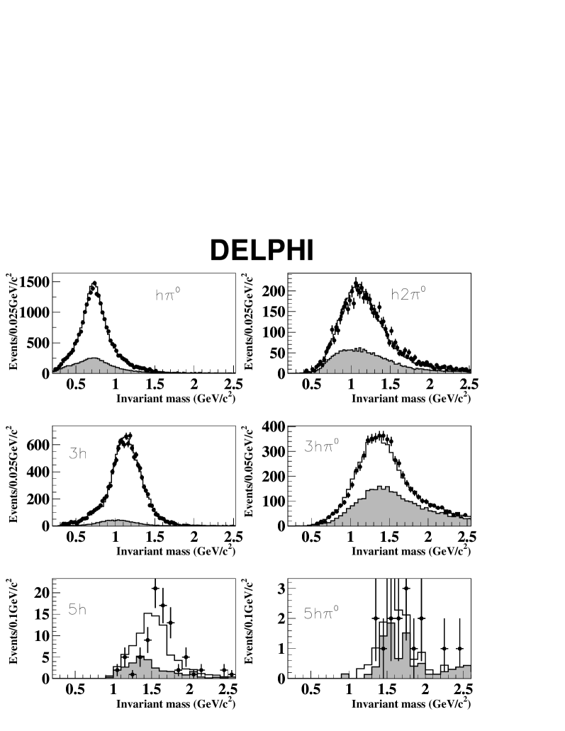
Figure 14: Invariant-mass distributions for the decays selected with sequential cuts, excluding the cuts directly related to this variable. Data are shown as dots, simulation by a solid line. The shaded area shows the background prediction from simulation.

The $h^{-}\pi^{0}$ invariant-mass distribution, calculated assuming the pion mass for the charged particle, is shown in Fig. 14. To reduce background it was required that the reconstructed $h^{-}\pi^{0}$ invariant mass lie in the range $0.48~{}$GeV$/c^{2}$ to $1.20~{}$GeV$/c^{2}$ and that the angle between the charged-particle direction and the $\pi^{0}$ direction be less than 20^∘.

The $\tau$-decay to $h^{-}\geq\!2\pi^{0}\nu_{\tau}$ was selected by requiring an isolated charged particle with two or more accompanying $\pi^{0}$ candidates. The charged particle had to have a reconstructed momentum greater than 0.5 GeV/$c$. The candidate $\pi^{0}$’s were reconstructed as described in Section 4.2.6. Furthermore, decays with only one reconstructed $\pi^{0}$ candidate were accepted if there was at least one well-reconstructed photon candidate (as described in Section 4.2) which was not used in the reconstruction of a $\pi^{0}$.

This semi-exclusive mode had little background from non-$\tau$ sources or from $\tau$-decay modes containing electrons and muons. The background was dominated by the $h^{-}\pi^{0}\nu_{\tau}$ decay mode. Further rejection of the background was performed by requiring that the invariant mass of the $h^{-}\pi^{0}\pi^{0}$ system be greater than 0.8 GeV/$c^{2}$ and that the total reconstructed energy be greater than 10 GeV. The pion mass was assumed for the charged particle and the $\pi^{0}$ mass for the $\pi^{0}$ candidate(s).

7.1.2 Three-prong decays

The signature of the decay $\tau^{-}\rightarrow 2h^{-}h^{+}\nu_{\tau}$ is of three charged particles with no accompanying electromagnetic showers. A candidate $2h^{-}h^{+}\nu_{\tau}$ decay had to have three charged-particle tracks in a hemisphere. The vector sum of the three charged-particle momenta had to have a magnitude greater than $0.166\times\sqrt{s}$. It was required that there be no reconstructed photon of energy greater than 1.5 GeV within $10^{\circ}$ of the three-charged-particle system momentum vector and that the total neutral electromagnetic energy in a cone of half-angle 10^∘ around the three-charged-particle system be less than 0.3 times the momentum of the three-charged-particle system. To reject cases where a photon or $\pi^{0}$ was associated to a charged-particle track extrapolation in the HPC it was required that the total energy associated to the three tracks in the first five layers of the HPC be less than 0.3 times the momentum of the three-charged-particle system.

The $\tau$-decay to $2h^{-}h^{+}\geq 1\pi^{0}\nu_{\tau}$ was selected by requesting three charged-particle tracks together with a $\pi^{0}$ candidate. The $\pi^{0}$ candidate had to lie in the barrel region, $|\cos\theta|<0.732$, within a cone of half-angle $30^{\circ}$ about the highest-momentum charged particle.

7.1.3 Five-prong decays

The exclusive decays $\tau^{-}\rightarrow 3h^{-}2h^{+}\nu_{\tau}$ and $\tau^{-}\rightarrow 3h^{-}2h^{+}\pi^{0}\nu_{\tau}$ were selected from the inclusive five-prong sample.

Decays with a total momentum greater than 40 GeV/$c$, an invariant mass of the five-charged-particle system greater than 1.5 GeV/$c^{2}$ or in which all photons had an energy less than 1.5 GeV were considered as $\tau^{-}\rightarrow 3h^{-}2h^{+}\nu_{\tau}$ decays. Otherwise the decay was classified as $\tau^{-}\rightarrow 3h^{-}2h^{+}\pi^{0}\nu_{\tau}$.

7.1.4 Results of the sequential-cuts analysis

The branching ratios were extracted from the data with a maximum-likelihood fit as described in Section 3.

The numbers of candidate $\tau$-decays in each class are given in Table 5, together with the branching ratio obtained. The uncertainties quoted are statistical and take into account correlations between different channels.

decay mode	Number	branching ratio (%)
$h^{-}\nu_{\tau}$	9727	12.765$\pm$	0.129
$h^{-}\pi^{0}\nu_{\tau}$	21098	26.243$\pm$	0.227
$h^{-}\!\!\geq\!\!2\pi^{0}\nu_{\tau}$	6187	10.928$\pm$	0.193
$3h^{\pm}\nu_{\tau}$	12761	9.352$\pm$	0.097
$3h^{\pm}\!\!\geq\!\!1\pi^{0}\nu_{\tau}$	5363	5.162$\pm$	0.091
$5h^{\pm}\nu_{\tau}$	96	0.097$\pm$	0.015
$5h^{\pm}\!\!\geq\!\!1\pi^{0}\nu_{\tau}$	13	0.016$\pm$	0.012

Table 5: For the sequential-cuts analysis, the numbers of selected events in each class and branching ratios obtained. The quoted uncertainties are statistical only.

The invariant-mass distributions of the different classes of selected decays are shown in Fig. 14 for all cuts applied except those directly related to the mass.

7.2 Neural-Net Analysis

The decay modes were also selected with the help of neural networks. Two different neural networks were designed, one for one-prong decays and another for three-prongs. They are described in this section. The events were initially separated according to their track multiplicity and then the selection with the corresponding neural net was applied. For five-prongs the sequential-cut analysis described in Sec.7.1.3 was applied.

7.2.1 One-prong decays

For the one-prong decay modes, a total of 43 input variables that could help the identification were studied: general variables (such as neutral multiplicities, invariant masses, and number of identified $\pi^{0}$), charged-particle variables (such as momentum, $dE/dx$, and calorimetric energies) or neutral-particle quantities (such as energy, and shower-profile variables). This number was reduced first using a principal-component analysis, removing linearly-redundant variables after testing that they did not affect the performance. Then, the network was trained and tested with and without variables which appeared to be less significant; they were removed if the results were not degraded. Finally, 15 variables were used as input. These variables were:

• the total invariant mass including charged and neutral particles;

• the number of reconstructed photons;

• the number of reconstructed $\pi^{0}$;

• the number of reconstructed photons not linked to any $\pi^{0}$;

• the magnitude of the momentum of the charged particle;

• the polar angle of the charged particle;

• the azimuthal angle, modulo 15^∘, of the extrapolation of the charged-particle track to the HPC;

• the pion hypothesis $dE/dx$ pull variable, $\Pi_{dE/dx}^{\pi}$;

• the number of muon chamber layers with hits associated to the charged particle;

• the number of muon chamber outer layers with hits associated to the charged particle;

• the total electromagnetic energy deposited in a cone of half-angle 30^∘ around the charged-particle track;

• the energy in the HPC associated to the charged particle;

• the energy in the inner four layers of the HPC associated to the charged particle;

• the total hadron calorimetric energy associated to the charged particle;

• the number of layers in the HCAL associated to the charged particle.

A feed-forward neural network [19] with one input layer, one hidden layer and one output layer was used. The input layer had 15 neurons, each one corresponding to one of the variables listed above. All the input variables were normalised to the range $[-1,1]$. Several structures were tested. Finally a net with one hidden layer of 40 neurons was used as the optimum in terms of efficiency and simplicity. The output layer consisted of six neurons. The assigned target value of these neurons was +1 for the corresponding class and $-1$ for the rest. Each neuron corresponded to one of the following decay modes: $\rm e^{-}\nu_{\tau}\bar{\nu}_{\mathrm{e}}$; $\mu^{-}\nu_{\tau}\bar{\nu}_{\mu}$; $h^{-}\nu_{\tau}$; $h^{-}\pi^{0}\nu_{\tau}$; $h^{-}\pi^{0}\pi^{0}\nu_{\tau}$; $h^{-}\geq\!3\pi^{0}\nu_{\tau}$.

A training procedure was performed on about 3000 simulated events for each of the classes, optimising the network parameters to give an answer in the output layer as close as possible to $+1$ in the neuron corresponding to the generated class and $-1$ in all others.

The total sample of simulated events, excluding those used for the training, was used to evaluate the probabilities that a given decay be identified in a given class. The selection efficiencies of the different classes and the misidentification probabilities are shown in Table 6.

true $\tau$	Neural network decay classification
decay mode	$\rm e^{-}\nu_{\tau}\bar{\nu}_{\mathrm{e}}$		$\mu^{-}\nu_{\tau}\bar{\nu}_{\mu}$		$h^{-}\nu_{\tau}$		$h^{-}\pi^{0}\nu_{\tau}$		$h^{-}2\pi^{0}\nu_{\tau}$		$h^{-}\!\!\geq\!\!3\pi^{0}\nu_{\tau}$
$\rm e^{-}\nu_{\tau}\bar{\nu}_{\mathrm{e}}$	89.86$\pm$	0.06	0.02$\pm$	0.00	1.32$\pm$	0.02	0.51$\pm$	0.01	0.16$\pm$	0.01	0.01$\pm$	0.00
$\mu^{-}\nu_{\tau}\bar{\nu}_{\mu}$	0.10$\pm$	0.01	88.02$\pm$	0.07	2.50$\pm$	0.03	0.41$\pm$	0.01	0.01$\pm$	0.00	0.00$\pm$	0.00
$\pi^{-}\nu_{\tau}$	2.07$\pm$	0.04	1.80$\pm$	0.04	78.59$\pm$	0.11	5.15$\pm$	0.06	0.22$\pm$	0.01	0.02$\pm$	0.00
$K^{-}\nu_{\tau}$	0.46$\pm$	0.07	3.33$\pm$	0.19	82.95$\pm$	0.40	5.84$\pm$	0.25	0.27$\pm$	0.06	0.04$\pm$	0.02
$\pi^{-}K^{0}_{\!\mathrm{L}}\nu_{\tau}$	1.32$\pm$	0.16	1.80$\pm$	0.18	68.45$\pm$	0.67	14.60$\pm$	0.59	1.46$\pm$	0.16	0.14$\pm$	0.05
$K^{-}K^{0}_{\!\mathrm{L}}\nu_{\tau}$	0.57$\pm$	0.23	1.85$\pm$	0.41	74.51$\pm$	1.46	11.83$\pm$	1.26	1.44$\pm$	0.36	0.00$\pm$	0.09
$\pi^{-}K^{0}_{\!\mathrm{S}}\nu_{\tau}$	5.49$\pm$	0.31	1.43$\pm$	0.16	38.08$\pm$	0.62	20.92$\pm$	0.64	6.57$\pm$	0.34	0.40$\pm$	0.09
$K^{-}K^{0}_{\!\mathrm{S}}\nu_{\tau}$	4.68$\pm$	0.65	3.77$\pm$	0.58	36.16$\pm$	1.35	20.84$\pm$	1.42	6.41$\pm$	0.75	0.59$\pm$	0.23
$\pi^{-}K^{0}_{\!\mathrm{L}}K^{0}\nu_{\tau}$	3.29$\pm$	0.53	1.10$\pm$	0.31	38.84$\pm$	1.34	25.56$\pm$	1.41	6.40$\pm$	0.72	1.86$\pm$	0.40
$\pi^{-}2K^{0}_{\!\mathrm{S}}\nu_{\tau}$	6.36$\pm$	1.26	0.72$\pm$	0.44	17.37$\pm$	1.35	22.23$\pm$	2.42	10.35$\pm$	1.57	2.28$\pm$	0.77
$\pi^{-}\pi^{0}\nu_{\tau}$	1.18$\pm$	0.02	0.43$\pm$	0.01	7.40$\pm$	0.05	68.51$\pm$	0.08	7.04$\pm$	0.05	0.20$\pm$	0.01
$K^{-}\pi^{0}\nu_{\tau}$	0.94$\pm$	0.12	1.09$\pm$	0.13	11.18$\pm$	0.38	66.57$\pm$	0.57	5.63$\pm$	0.28	0.25$\pm$	0.06
$\pi^{-}\pi^{0}K^{0}_{\!\mathrm{L}}\nu_{\tau}$	0.61$\pm$	0.16	0.21$\pm$	0.09	5.19$\pm$	0.45	64.99$\pm$	0.96	13.57$\pm$	0.69	1.19$\pm$	0.22
$K^{-}\pi^{0}K^{0}_{\!\mathrm{L}}\nu_{\tau}$	0.55$\pm$	0.25	0.45$\pm$	0.22	13.48$\pm$	1.13	57.61$\pm$	1.64	9.49$\pm$	0.97	0.73$\pm$	0.28
$\pi^{-}\pi^{0}K^{0}_{\!\mathrm{S}}\nu_{\tau}$	2.12$\pm$	0.29	0.72$\pm$	0.17	4.38$\pm$	0.42	40.91$\pm$	1.00	21.23$\pm$	0.84	3.41$\pm$	0.37
$K^{-}\pi^{0}K^{0}_{\!\mathrm{S}}\nu_{\tau}$	3.56$\pm$	0.67	2.57$\pm$	0.57	7.06$\pm$	0.92	41.17$\pm$	1.77	13.52$\pm$	1.23	3.32$\pm$	0.64
$\pi^{-}2\pi^{0}\nu_{\tau}$	0.84$\pm$	0.02	0.15$\pm$	0.01	1.39$\pm$	0.03	33.92$\pm$	0.13	38.33$\pm$	0.13	4.22$\pm$	0.05
$K^{-}2\pi^{0}\nu_{\tau}$	0.84$\pm$	0.29	0.42$\pm$	0.20	1.35$\pm$	0.36	35.18$\pm$	1.49	35.45$\pm$	1.49	3.92$\pm$	0.60
$\pi^{-}3\pi^{0}\nu_{\tau}$	0.62$\pm$	0.06	0.07$\pm$	0.02	0.69$\pm$	0.07	18.76$\pm$	0.32	42.33$\pm$	0.41	15.97$\pm$	0.30
$2\pi^{-}\pi^{+}\nu_{\tau}$	0.08$\pm$	0.01	0.03$\pm$	0.00	0.29$\pm$	0.01	2.03$\pm$	0.03	0.26$\pm$	0.01	0.02$\pm$	0.00
$K^{-}\pi^{-}\pi^{+}\nu_{\tau}$	0.13$\pm$	0.05	0.03$\pm$	0.03	0.33$\pm$	0.09	1.79$\pm$	0.20	0.18$\pm$	0.07	0.02$\pm$	0.02
$K^{-}K^{+}\pi^{+}\nu_{\tau}$	0.17$\pm$	0.08	0.05$\pm$	0.04	0.31$\pm$	0.10	1.64$\pm$	0.23	0.17$\pm$	0.08	0.00$\pm$	0.03
$2\pi^{-}\pi^{+}\pi^{0}\nu_{\tau}$	0.09$\pm$	0.01	0.01$\pm$	0.00	0.10$\pm$	0.01	1.70$\pm$	0.05	1.60$\pm$	0.05	0.20$\pm$	0.02
$3\pi^{\pm}2\pi^{0}\nu_{\tau}$	0.06$\pm$	0.03	0.02$\pm$	0.02	0.03$\pm$	0.02	1.08$\pm$	0.12	2.13$\pm$	0.17	1.09$\pm$	0.12
$3\pi^{\pm}3\pi^{0}\nu_{\tau}$	0.00$\pm$	0.08	0.00$\pm$	0.08	0.08$\pm$	0.08	0.23$\pm$	0.14	2.30$\pm$	0.43	2.75$\pm$	0.47
$3\pi^{-}2\pi^{+}\nu_{\tau}$	0.00$\pm$	0.21	0.00$\pm$	0.21	0.00$\pm$	0.21	0.32$\pm$	0.26	0.12$\pm$	0.21	0.00$\pm$	0.21
$3\pi^{-}2\pi^{+}\pi^{0}\nu_{\tau}$	0.00$\pm$	0.83	0.00$\pm$	0.83	0.00$\pm$	0.83	1.00$\pm$	0.91	0.00$\pm$	0.83	0.00$\pm$	0.83
Source	Non-$\tau^{+}\tau^{-}$ backgrounds
$\mu^{+}\mu^{-}$	0.03$\pm$	0.01	0.39$\pm$	0.02	0.02$\pm$	0.00	0.06$\pm$	0.01	0.05$\pm$	0.01	0.00$\pm$	0.00
${\rm e}^{+}{\rm e}^{-}$	1.27$\pm$	0.19	0.01$\pm$	0.01	0.16$\pm$	0.03	0.06$\pm$	0.01	0.05$\pm$	0.02	0.08$\pm$	0.08
${\rm q}\bar{\rm q}$	0.02$\pm$	0.01	0.07$\pm$	0.01	0.09$\pm$	0.02	0.15$\pm$	0.02	0.11$\pm$	0.03	0.26$\pm$	0.13
4f	1.91$\pm$	0.19	0.84$\pm$	0.08	0.37$\pm$	0.05	0.44$\pm$	0.04	0.25$\pm$	0.05	0.18$\pm$	0.13

Table 6: For the neural-networks analysis, the top part contains estimates of classification efficiencies, in percent, for different exclusive one-prong decay modes, as obtained from simulation after correction for the data/simulation discrepancies discussed in the text. The bottom part shows backgrounds from non-$\tau^{+}\tau^{-}$ sources. The quoted uncertainties are from the simulation statistics only. When no events are classified in a given class the Poissonian upper bound is taken as error. Numbers smaller than 0.005% are represented in the table as 0.00.

Each of the preselected one-prong decays was processed through the neural network and the decay was identified as belonging to the class whose corresponding output was largest. Events with no output neuron above zero were not classified. The number of events with two or more output neurons above zero was negligible.

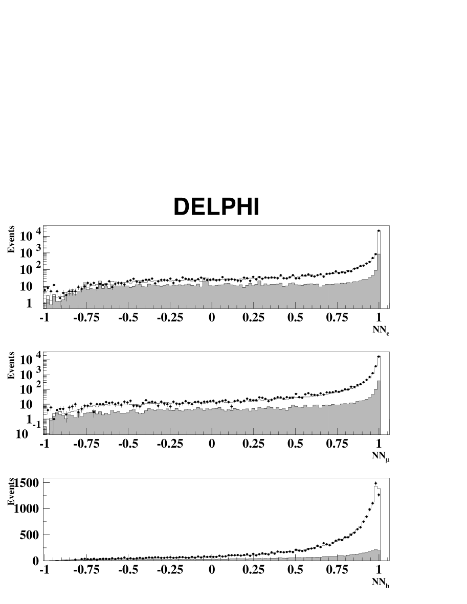
Figure 15: Maximum-output neuron value in one-prong analyses. For each event the output of the class whose output neuron is maximum is represented. Data are shown as dots and simulation by a solid line. The shaded area represents the background events.

The distributions of the maximum value of the output neuron for each decay mode for all decays are shown in Figs. 15 and  16. In most cases, this shows satisfactory agreement between data and simulation.

7.2.2 Three-prong decays

The three-prong $\tau$-decay candidates selected were divided into three classes: $2h^{-}h^{+}\nu_{\tau}$, $2h^{-}h^{+}\pi^{0}\nu_{\tau}$ and $2h^{-}h^{+}\geq 2\pi^{0}\nu_{\tau}$.

A simpler network was used in this case, with all the electron/muon/hadron-identification variables removed and the remaining variables kept, giving a total of seven variables:

• the total momentum of the charged-particle system;

• the total electromagnetic energy associated to the charged-particle tracks;

• the total electromagnetic energy deposited in a cone of half-angle 15^∘ around the momentum vector of the charged-particle system including that associated to the charged-particle tracks;

• the number of reconstructed photons;

• the number of reconstructed $\pi^{0}$;

• the number of reconstructed photons not used in a reconstructed $\pi^{0}$;

• the total invariant mass.

The photons and $\pi^{0}$ had to lie in a cone of half-angle 30^∘ about the highest-momentum charged particle. The hidden layer had 15 neurons and three output neurons were used. The network was trained with 3000 events of each of the signal classes optimising the network as for the one-prongs, to give outputs close to $+1$ in the neuron corresponding to the generated class and $-1$ in the others. Here, to reduce the background from other decays, the network was also trained with 3000 one-prong events that fulfilled the three-prong selection requirements, to give answers as close to $-1$ in all the output neurons.

The event classification from the output neuron values was performed in an equivalent way to the one-prong case. The efficiencies and background levels for the different decay classes are given in Table 7.

true $\tau$	Neural network decay classification
decay mode	$3h^{\pm}\nu_{\tau}$		$3h^{\pm}\pi^{0}\nu_{\tau}$		$3h^{\pm}\!\!\geq\!\!2\pi^{0}\nu_{\tau}$		Unclassified
$\rm e^{-}\nu_{\tau}\bar{\nu}_{\mathrm{e}}$	0.01$\pm$	0.00	0.01$\pm$	0.00	0.00$\pm$	0.00	8.11$\pm$	0.06
$\mu^{-}\nu_{\tau}\bar{\nu}_{\mu}$	0.03$\pm$	0.00	0.00$\pm$	0.00	0.00$\pm$	0.00	8.92$\pm$	0.06
$\pi^{-}\nu_{\tau}$	0.08$\pm$	0.01	0.03$\pm$	0.00	0.00$\pm$	0.00	12.04$\pm$	0.09
$K^{-}\nu_{\tau}$	0.07$\pm$	0.03	0.01$\pm$	0.01	0.00$\pm$	0.01	7.03$\pm$	0.27
$\pi^{-}K^{0}_{\!\mathrm{L}}\nu_{\tau}$	0.12$\pm$	0.05	0.06$\pm$	0.03	0.00$\pm$	0.02	12.05$\pm$	0.44
$K^{-}K^{0}_{\!\mathrm{L}}\nu_{\tau}$	0.05$\pm$	0.09	0.13$\pm$	0.11	0.04$\pm$	0.09	9.56$\pm$	0.90
$\pi^{-}K^{0}_{\!\mathrm{S}}\nu_{\tau}$	4.03$\pm$	0.27	1.07$\pm$	0.14	0.00$\pm$	0.02	21.99$\pm$	0.57
$K^{-}K^{0}_{\!\mathrm{S}}\nu_{\tau}$	3.90$\pm$	0.59	1.01$\pm$	0.31	0.14$\pm$	0.12	22.50$\pm$	1.28
$\pi^{-}K^{0}_{\!\mathrm{L}}K^{0}\nu_{\tau}$	2.24$\pm$	0.44	1.30$\pm$	0.33	0.49$\pm$	0.21	18.92$\pm$	1.16
$\pi^{-}2K^{0}_{\!\mathrm{S}}\nu_{\tau}$	6.41$\pm$	1.27	6.47$\pm$	1.27	0.77$\pm$	0.45	27.05$\pm$	2.30
$\pi^{-}\pi^{0}\nu_{\tau}$	0.41$\pm$	0.01	0.73$\pm$	0.02	0.07$\pm$	0.00	14.01$\pm$	0.06
$K^{-}\pi^{0}\nu_{\tau}$	0.44$\pm$	0.08	0.92$\pm$	0.12	0.12$\pm$	0.04	12.84$\pm$	0.41
$\pi^{-}\pi^{0}K^{0}_{\!\mathrm{L}}\nu_{\tau}$	0.22$\pm$	0.10	1.15$\pm$	0.21	0.15$\pm$	0.08	12.71$\pm$	0.67
$K^{-}\pi^{0}K^{0}_{\!\mathrm{L}}\nu_{\tau}$	0.79$\pm$	0.29	1.46$\pm$	0.40	0.11$\pm$	0.11	15.34$\pm$	1.20
$\pi^{-}\pi^{0}K^{0}_{\!\mathrm{S}}\nu_{\tau}$	0.39$\pm$	0.13	5.45$\pm$	0.46	0.41$\pm$	0.13	20.98$\pm$	0.83
$K^{-}\pi^{0}K^{0}_{\!\mathrm{S}}\nu_{\tau}$	1.29$\pm$	0.41	5.00$\pm$	0.78	0.15$\pm$	0.14	22.37$\pm$	1.50
$\pi^{-}2\pi^{0}\nu_{\tau}$	0.27$\pm$	0.01	2.20$\pm$	0.04	0.75$\pm$	0.02	17.93$\pm$	0.10
$K^{-}2\pi^{0}\nu_{\tau}$	0.22$\pm$	0.15	2.38$\pm$	0.48	0.62$\pm$	0.24	19.62$\pm$	1.24
$\pi^{-}3\pi^{0}\nu_{\tau}$	0.10$\pm$	0.03	2.05$\pm$	0.12	1.73$\pm$	0.11	17.69$\pm$	0.31
$2\pi^{-}\pi^{+}\nu_{\tau}$	78.11$\pm$	0.09	14.10$\pm$	0.08	0.24$\pm$	0.01	4.84$\pm$	0.05
$K^{-}\pi^{-}\pi^{+}\nu_{\tau}$	77.79$\pm$	0.64	14.21$\pm$	0.54	0.18$\pm$	0.07	5.34$\pm$	0.35
$K^{-}K^{+}\pi^{+}\nu_{\tau}$	74.53$\pm$	0.80	15.72$\pm$	0.67	0.26$\pm$	0.09	7.17$\pm$	0.48
$2\pi^{-}\pi^{+}\pi^{0}\nu_{\tau}$	16.51$\pm$	0.16	69.06$\pm$	0.19	3.62$\pm$	0.08	6.99$\pm$	0.11
$3\pi^{\pm}2\pi^{0}\nu_{\tau}$	4.31$\pm$	0.24	59.12$\pm$	0.57	24.80$\pm$	0.50	7.22$\pm$	0.30
$3\pi^{\pm}3\pi^{0}\nu_{\tau}$	1.63$\pm$	0.36	40.66$\pm$	1.41	46.68$\pm$	1.43	5.51$\pm$	0.65
$3\pi^{-}2\pi^{+}\nu_{\tau}$	18.47$\pm$	1.76	19.64$\pm$	1.80	0.51$\pm$	0.32	2.05$\pm$	0.64
$3\pi^{-}2\pi^{+}\pi^{0}\nu_{\tau}$	4.68$\pm$	1.93	30.12$\pm$	4.19	3.21$\pm$	1.61	7.72$\pm$	2.44
Source	Non-$\tau^{+}\tau^{-}$ backgrounds
$\mu^{+}\mu^{-}$	0.00$\pm$	0.00	0.00$\pm$	0.00	0.00$\pm$	0.00	0.24$\pm$	0.02
${\rm e}^{+}{\rm e}^{-}$	0.00$\pm$	0.00	0.00$\pm$	0.00	0.00$\pm$	0.00	0.60$\pm$	0.09
${\rm q}\bar{\rm q}$	0.75$\pm$	0.05	1.89$\pm$	0.12	5.11$\pm$	0.67	1.07$\pm$	0.11
4f	0.26$\pm$	0.04	0.22$\pm$	0.05	0.82$\pm$	0.33	0.53$\pm$	0.04

Table 7: For the neural-networks analysis, classification efficiencies, in percent, for different exclusive three-prong decay modes, as obtained from simulation after correction for the data/simulation discrepancies discussed in the text. The last column represents the percentage of events not classified in any of the classes by the neural network, including the sequential-cuts selection of five-prong modes. The bottom part shows backgrounds in percent in each class from non-$\tau^{+}\tau^{-}$ sources. The quoted uncertainties are from the simulation statistics only. When no events are classified in a given class the Poissonian upper bound is taken as error. Numbers smaller than 0.005% are represented in the table as 0.00.

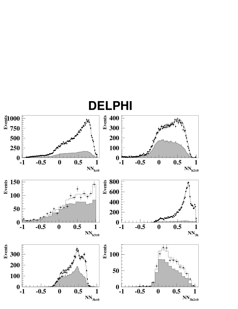
Figure 16: Maximum-output neuron value in one-prong and three-prong neural-net analyses. For each event the output of the class whose output neuron is maximum is represented. Data are shown as dots and simulation by a solid line. The shaded area represents the background events.

The distributions of the largest value of the output neurons in each decay are shown in Fig. 16, showing in most cases good agreement in shape between data and simulation.

7.2.3 Results of the neural-network analysis

As explained in Section 3, a simultaneous fit for the branching ratios was performed by fitting the predicted number of candidate $\tau$-decays in each class to the observed number. In this case, the information of the neural-net output was also used in the fit, where the sum over classes was extended to run over classes and bins in the neural-net output. Only positive values of this output were taken into account for the quoted results. The minimum value used in the fit was varied through the full range from $-1$ to $\mathrm{𝟎}$ without any variation on the branching ratio obtained, beyond that expected from statistical fluctuations. For the five-prong case the sequential-cuts analysis was used. The numbers of selected candidate $\tau$-decays in each class are given in Table 8, together with the branching ratio obtained. The uncertainties quoted are statistical and take into account correlations between different channels. Despite the fact that the fit was not minimizing a $\chi^{2}$, it was a maximum-likelihood fit, a $\chi^{2}$ is calculated to estimate of the goodness of the fit. Accounting only for statistical errors, a $\chi^{2}=808$ for 490 $d.o.f.$ was obtained, with the contribution from each channel presented in Table 8. The effect of systematic errors on the $\chi^{2}$ will be discussed in Section 8.10.

decay mode	Number	branching ratio		$\chi^{2}$ (bins)
$e^{-}\nu_{\tau}\nu_{\rm e}$	25529	17.803$\pm$	0.108	54.9 (	55 )
$\mu^{-}\nu_{\tau}\nu_{\mu}$	25860	17.350$\pm$	0.104	160.1 (	55 )
$h^{-}\nu_{\tau}$	19212	12.780$\pm$	0.120	68.6 (	55 )
$h^{-}\pi^{0}\nu_{\tau}$	34675	26.291$\pm$	0.201	85.1 (	55 )
$h^{-}2\pi^{0}\nu_{\tau}$	9504	9.524$\pm$	0.320	59.0 (	55 )
$h^{-}\!\!\geq\!\!3\pi^{0}\nu_{\tau}$	1083	1.403$\pm$	0.214	92.1 (	55 )
$3h^{\pm}\nu_{\tau}$	12176	9.340$\pm$	0.090	152.5 (	55 )
$3h^{\pm}\pi^{0}\nu_{\tau}$	8909	4.545$\pm$	0.106	77.8 (	55 )
$3h^{\pm}\!\!\geq\!\!2\pi^{0}\nu_{\tau}$	1272	0.561$\pm$	0.068	51.1 (	55 )
$5h^{\pm}\nu_{\tau}$	96	0.097$\pm$	0.015	0.0 (	1 )
$5h^{\pm}\!\!\geq\!\!1\pi^{0}\nu_{\tau}$	13	0.016$\pm$	0.012	1.7 (	1 )

unclassified	Number	expected		$\chi^{2}$ (bins)
1-prong	18558	18857.7		2.2 (	1 )
3-prong	1517	1455.1		1.6 (	1 )
5-prong	3	5.2		1.6 (	1 )

Table 8: For the neural-networks analysis, numbers of selected events in each class and branching ratios obtained. The quoted uncertainties are statistical only. The last column shows the contribution of each to the total $\chi^{2}$, computed with statistical errors only. In parenthesis is shown the number of data points used in each case. The last three lines compare the measured number of unclassified events with the expectation after the fit.

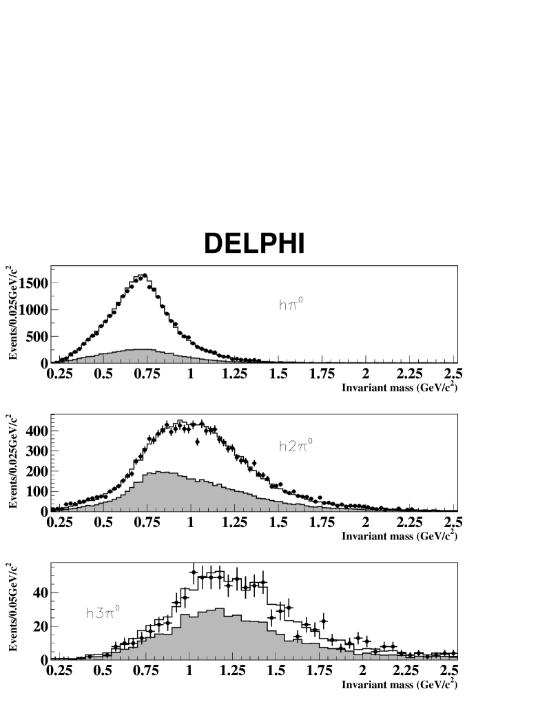
Figure 17: Invariant-mass distributions for the one-prong decays selected with the neural network. Data are shown as dots, simulation by a solid line. The shaded area shows the background prediction from simulation.

The invariant-mass distributions of the different classes of selected decays are shown in Figs. 17 and  18.

8 Systematics

The systematic uncertainties due to any specific source were estimated simultaneously for all measured decay modes in the neural-network and sequential-cuts analyses. This was also the case for inclusive branching ratios, where the calculated systematic errors accounted for the existing cancellations between the errors of the different channels involved, leading in many cases to smaller errors.

The systematic errors were evaluated using test samples of events as discussed in Sections 4.1 and 4.2. Where appropriate the relevant input variables were varied by the observed uncertainty and the selection and fit were repeated. The variation in the results was taken as an estimate of the systematic effect on the branching ratios. The effects of the external background and the preselection efficiency were also checked. The potential sources of systematic uncertainties are discussed below and summarised in Table 9.

8.1 $\tau^{+}\tau^{-}$ selection and non-$\tau^{+}\tau^{-}$ backgrounds

The background levels from channels other than $\tau^{+}\tau^{-}$ were varied by the uncertainties given in Section 5 and the fit was repeated. The observed changes on the results for the variation in each of the background types were added in quadrature to obtain the estimate of the systematic error.

The probability of identifying a hemisphere from a background event in a given class was checked with the electron and muon test samples described in Section 4. The ${\rm q}\bar{\rm q}$ background was checked with low-multiplicity ${\rm q}\bar{\rm q}$ test samples selected applying the $\tau^{+}\tau^{-}$ selection, except the isolation cut, which was changed to $120^{\circ}<\theta_{iso}<150^{\circ}$. The classification rates were compared between real and simulated data and the systematic error was estimated conservatively as the largest of the statistical error and the difference between both.

8.2 Charged-particle reconstruction

The sources of systematic uncertainty associated with the charged-particle multiplicity selection have been studied in [16]. For track reconstruction, the sources investigated include: the efficiencies of the different tracking subdetectors to be included on a reconstructed track, both for isolated tracks and for tracks in higher track density topologies; effects of the TPC inter-sector boundary regions; the two-track resolution of the tracking system and the efficiency to reconstruct a multi-prong $\tau$-decay as a function of the minimum opening angle between any two particles; the candidate $\tau$ charge reconstruction.

8.3 Material reinteractions

Uncertainties from the photon conversion reconstruction were particularly important for those decay modes containing $\pi^{0}$’s. The effect on the branching ratios was estimated by varying by their uncertainties the correction factors for the reconstructed and unreconstructed conversions given in Table 1 of [16], which were obtained from data test samples of radiative dilepton events. The resultant uncertainties are dominated by the contribution from the unreconstructed conversions. A similar approach was taken for the nuclear interactions, with the correction factors given by Table 2 in [16].

8.4 Relative efficiency of exclusive modes

Due to mass effects and decay dynamics the momentum distributions of $\pi^{\pm}$ and $K^{\pm}$ are different even for otherwise identical final states.

To estimate the size of these effects the proportions of charged pions and kaons in a given decay mode were varied by an amount consistent with the uncertainties quoted in the Particle Data Listings [18], the selection efficiency for that class recalculated and the fit repeated. The change in the measured branching ratio was taken as the systematic uncertainty.

Within many classes there were a number of exclusive decay modes which differ in $K^{0}$ multiplicity, and which may not have the same selection efficiency. To estimate the uncertainty on the measured branching ratios, the exclusive branching ratios in a given class were varied within the uncertainties quoted in the Particle Data Listings [18]. The uncertainty on the three-prong modes also included a contribution due to the decay modes $K^{-}\pi^{-}\pi^{+}\pi^{0}\nu_{\tau}$ and $K^{-}K^{+}\pi^{-}\pi^{0}\nu_{\tau}$ which were not included in the simulation.

Similarly, the decays containing $\eta$ and $\omega$ mesons were varied by the uncertainties on the world average to obtain systematic uncertainties on the measured branching ratios.

8.5 Decay modelling

The uncertainties associated with the modelling of the decays involving several pions or kaons were estimated by correcting the efficiencies taking into account differences between data and simulated invariant-mass distributions. In addition, the hadronic structure of the $3\pi$ final state was varied between the default TAUOLA [14] model and that obtained in the DELPHI analysis of the $3\pi$ structure in $\tau$-decays [20]. For the $3\pi\pi^{0}$ structure the parameterisation of Model 1 of [21] was used and, as a cross-check, the parameterisation of $3\pi\pi^{0}$ used in [20] was used to reweight the distributions of the minimum opening angle.

The charged particle(s) produced in the various $\tau$-decay modes have different momentum spectra for the different helicity states. This leads to differences in acceptance as a function of the $\tau$ polarisation due to cuts in the $\tau^{+}\tau^{-}$ selection. This is especially the case for $\tau\to\pi\nu_{\tau},K\nu_{\tau}$ where the momentum spectra differ most between the two helicity states. The analysis used the result and uncertainty from the DELPHI analysis on $\tau$ polarisation [22].

8.6 Trigger

The trigger efficiency for $\tau^{+}\tau^{-}$ final states was $(99.98\pm 0.01)$% for events within the polar-angle acceptance. Studies indicated that this inefficiency was due to events where both $\tau$’s decayed via the $\tau\to\mu\nu\nu$ mode. This can be extrapolated to an inefficiency of $(6\pm 3)\times 10^{-4}$ for the channel $\tau^{-}\rightarrow\mu^{-}\nu_{\tau}\bar{\nu}_{\mu}$. The associated systematic uncertainty was obtained by varying the inefficiency by its error.

8.7 Energy and momentum scale and resolution

The HPC energy scale was altered in the simulation by the uncertainty described in Section 4.2.4 and the complete analysis re-performed. The changes in the obtained branching ratios were taken as the uncertainty. In a similar manner the simulation energy was smeared and the branching ratios re-estimated. This took into account, with the correct correlation, different effects related to the electromagnetic calorimetry: ${\rm e}^{+}{\rm e}^{-}$ rejection, $\tau^{-}\rightarrow\rm e^{-}\nu_{\tau}\bar{\nu}_{\mathrm{e}}$ identification and rejection through $E_{ass}$, $\pi^{0}$ identification and total invariant masses. The same procedure was followed with the momentum scale and resolution as given in Section 4.1.1.

8.8 HCAL, muon chambers and dE/dx

The correction in simulation to the tails of hadronic showers in the HCAL and muon chambers was modified by the uncertainties derived in Section 4.1. The analysis was repeated, and the observed variations in the branching ratios obtained were taken as uncertainties.

The fraction of extra layers added in the simulation to give better data/simulation agreement was varied by the uncertainty obtained in Section 4.1 and the analysis repeated. The uncertainties were taken from the variations in the branching ratios obtained. For the tails of showers penetrating into the muon chambers, the efficiency was varied by the uncertainty observed in the test samples for both muons and hadrons.

In a similar way, the response of the HCAL and muon chambers for muons was varied within the uncertainties obtained in 4.1 with muon test samples.

The $dE/dx$ was varied in simulation for each particle according to the errors in the tuning described in 4.1 and the analysis re-performed. The uncertainties were taken from the changes in the branching ratios obtained. This affected mostly the $\tau^{-}\rightarrow\rm e^{-}\nu_{\tau}\bar{\nu}_{\mathrm{e}}$ and $\tau^{-}\rightarrow h^{-}\nu_{\tau}$ branching ratios whose separation depended most on $dE/dx$.

8.9 Photon and neutral-pion reconstruction

The photon efficiency, the probability to split one photon into two, the probability to create fake photons from a hadron, as well as the $\pi^{0}$ reconstruction efficiency and fake probability were checked with different test samples, as described in Section 4.2. The different errors were propagated to the efficiency tables and the fits were repeated. The observed difference was taken as systematic error.

8.10 Summary of systematic uncertainties

A contribution to the systematic uncertainty was included for the statistical uncertainty on the components of the selection-efficiency matrices due to the finite simulation sample size.

The systematic uncertainty associated with each source and for each measured decay mode is shown for the neural network analysis in Table 9. The total systematic error was calculated as the quadratic sum of these contributions, since they were essentially independent. The errors for the sequential-cuts analysis were similar, but slightly larger in general.

An attempt to estimate the effect of systematic errors on the goodness of the fit was made under the following procedure. The systematic errors were estimated bin by bin as the observed difference in the simulated distributions when the previously discussed systematic effects were varied within their uncertainties. A $\chi^{2}=397$ for 490 $d.o.f.$ was thus evaluated, neglecting the bin to bin correlations (which slightly underestimates the $\chi^{2}$). The major contributions to the $\chi^{2}$ reported in Table 8 came from distortions of the neural network output in regions far from the cut, and where the signal and background separation was very clear and therefore did not affect the results significantly compared to the quoted systematic errors. In particular, the largest contribution, arising from the $\tau^{-}\rightarrow\mu^{-}\nu_{\tau}\bar{\nu}_{\mu}$ channel is due to the slight widening of the sharp peak on the neural network output distribution (Fig. 15) caused by the HCAL and muon chamber response systematics, with a migration of a small fraction of events from values close to 1 to the region from 0.5 to 1. This has a large impact on the $\chi^{2}$, but very small one on the results, since they are nevertheless identified clearly. Similar arguments apply to the second largest contribution, from the $\tau^{-}\rightarrow 2h^{-}h^{+}\nu_{\tau}$, but in this case the neural network peak (Fig. 15) is narrower in data.

	1-prong decay mode
Source of systematic	$\rm e^{-}\nu_{\tau}\bar{\nu}_{\mathrm{e}}$	$\mu^{-}\nu_{\tau}\bar{\nu}_{\mu}$	$h^{-}\nu_{\tau}$	$h^{-}\pi^{0}\nu_{\tau}$	$h^{-}2\pi^{0}\nu_{\tau}$	$h^{-}\!\!\geq\!\!1\pi^{0}\nu_{\tau}$	$h^{-}\!\!\geq\!\!2\pi^{0}\nu_{\tau}$	$h^{-}\!\!\geq\!\!3\pi^{0}\nu_{\tau}$
Non-$\tau$ background scale	26	8	2	7	6	11	4	2
Non-$\tau$ background classification	9	3	3	8	2	8	2	5
Tracking and VD efficiency	10	3	15	33	121	70	50	93
Material reinteractions	16	12	13	38	28	25	48	28
Exclusive BRs	13	13	38	41	28	47	24	7
Decay modelling	1	2	1	17	22	8	13	10
Trigger	4	30	3	7	3	10	3	$<$1
Energy and momentum calibration	90	10	13	81	193	33	63	155
HCAL and muon chamber response	1	70	70	7	4	2	4	8
$dE/dx$ calibration	54	14	42	2	12	30	13	37
Photon and $\pi^{0}$ reconstruction	23	7	32	49	116	37	34	109
Simulation statistics	28	27	31	57	88	39	51	58
Total systematic	116	85	103	130	274	116	116	224

	3- or 5-prong decay mode
Source of systematic	$3h^{\pm}\nu_{\tau}$	$3h^{\pm}\pi^{0}\nu_{\tau}$	$3h^{\pm}\!\!\geq\!\!2\pi^{0}\nu_{\tau}$	$3h^{\pm}\!\!\geq\!\!1\pi^{0}\nu_{\tau}$	$5h^{\pm}\nu_{\tau}$	$5h^{\pm}\!\!\geq\!\!1\pi^{0}\nu_{\tau}$
Non-$\tau$ background scale	5	2	3	5	0	0
Non-$\tau$ background classification	4	18	40	40	0	0
Tracking and VD efficiency	15	30	29	70	2.3	5.1
material reinteractions	27	8	19	22	1.5	1.1
Exclusive BRs	11	39	30	23	0.0	0.0
Decay modelling	3	5	1	6	1.0	1.0
Trigger	3	2	0	2	0.0	0.0
Energy and momentum calibration	17	37	27	10	0.3	0.3
HCAL and muon chamber response	1	3	2	1	0.0	0.0
$dE/dx$ calibration	17	0	10	23	0.0	0.0
Photon and $\pi^{0}$ reconstruction	62	70	60	44	0.8	0.8
Simulation statistics	27	38	28	24	4.4	3.5
Total systematic	79	103	95	103	5.4	6.4

Table 9: Contributions in units of ${\mathit{10^{-5}}}$ to the systematic uncertainties on the branching ratios.

9 Results

The neural-network analysis gave for all hadronic channels better precision both in statistics and systematics, and included more channels. Therefore the results from this analysis were taken as the basic measurement, while the sequential analysis (except for the five-prong channels) was kept only as a cross-check. However, the performance for the leptonic decays is slightly worse than in [15] and therefore those results are not updated. Taking into account the statistical and systematic correlation of the channels with one or several $\pi^{0}$ some inclusive branching ratios were also derived.

The results are shown in Table 10.

Decay mode	Branching Ratio(%)
$\tau^{-}\to h^{-}\geq 0K^{0}\nu_{\tau}$	$12.780\pm 0.120\pm 0.103$
$\tau^{-}\to h^{-}\pi^{0}\geq 0K^{0}\nu_{\tau}$	$26.291\pm 0.201\pm 0.130$
$\tau^{-}\to h^{-}2\pi^{0}\geq 0K^{0}\nu_{\tau}$	$9.524\pm 0.320\pm 0.274$
$\tau^{-}\to h^{-}\geq 1\pi^{0}\geq 0K^{0}\nu_{\tau}$	$37.218\pm 0.155\pm 0.116$
$\tau^{-}\to h^{-}\geq 2\pi^{0}\geq 0K^{0}\nu_{\tau}$	$10.927\pm 0.173\pm 0.116$
$\tau^{-}\to h^{-}\geq 3\pi^{0}\geq 0K^{0}\nu_{\tau}$	$1.403\pm 0.214\pm 0.224$
$\tau^{-}\to 3h^{\pm}\geq 0K^{0}\nu_{\tau}$	$9.340\pm 0.090\pm 0.079$
$\tau^{-}\to 3h^{\pm}\pi^{0}\geq 0K^{0}\nu_{\tau}$	$4.545\pm 0.106\pm 0.103$
$\tau^{-}\to 3h^{\pm}\!\!\geq\!\!1\pi^{0}\geq 0K^{0}\nu_{\tau}$	$5.106\pm 0.083\pm 0.103$
$\tau^{-}\to 3h^{\pm}\!\!\geq\!\!2\pi^{0}\geq 0K^{0}\nu_{\tau}$	$0.561\pm 0.068\pm 0.095$
$\tau^{-}\to 5h^{\pm}\geq 0K^{0}\nu_{\tau}$	$0.097\pm 0.015\pm 0.005$
$\tau^{-}\to 5h^{\pm}\!\!\geq\!\!1\pi^{0}\geq 0K^{0}\nu_{\tau}$	$0.016\pm 0.012\pm 0.006$

Table 10: Measured branching ratios in percent. The uncertainties are statistical followed by systematic.

The correlation matrix for the combined statistical and systematic uncertainties is shown in Table 11.

	$h^{-}\nu_{\tau}$	$h^{-}\pi^{0}\nu_{\tau}$	$h^{-}\!\!\geq\!\!1\pi^{0}\nu_{\tau}$	$h^{-}2\pi^{0}\nu_{\tau}$	$h^{-}\!\!\geq\!\!2\pi^{0}\nu_{\tau}$	$h^{-}\!\!\geq\!\!3\pi^{0}\nu_{\tau}$	$3h^{\pm}\nu_{\tau}$	$3h^{\pm}\pi^{0}\nu_{\tau}$	$3h^{\pm}\!\!\geq\!\!1\pi^{0}\nu_{\tau}$	$3h^{\pm}\!\!\geq\!\!2\pi^{0}\nu_{\tau}$	$5h^{\pm}\nu_{\tau}$	$5h^{\pm}\!\!\geq\!\!1\pi^{0}\nu_{\tau}$
$h^{-}\pi^{0}\nu_{\tau}$	$-$0.34
$h^{-}\!\!\geq\!\!1\pi^{0}\nu_{\tau}$	$-$0.47	0.56
$h^{-}2\pi^{0}\nu_{\tau}$	0.06	$-$0.66	0.15
$h^{-}\!\!\geq\!\!2\pi^{0}\nu_{\tau}$	$-$0.03	$-$0.74	0.15	0.81
$h^{-}\!\!\geq\!\!3\pi^{0}\nu_{\tau}$	$-$0.06	0.38	0.11	$-$0.86	$-$0.36
$3h^{\pm}\nu_{\tau}$	$-$0.07	$-$0.08	0.15	0.00	$-$0.03	$-$0.02
$3h^{\pm}\pi^{0}\nu_{\tau}$	$-$0.02	$-$0.01	$-$0.05	$-$0.03	$-$0.02	0.03	$-$0.53
$3h^{\pm}\!\!\geq\!\!1\pi^{0}\nu_{\tau}$	$-$0.04	$-$0.04	$-$0.13	$-$0.04	$-$0.06	$-$0.02	$-$0.56	0.75
$3h^{\pm}\!\!\geq\!\!2\pi^{0}\nu_{\tau}$	$-$0.01	$-$0.01	$-$0.04	0.03	$-$0.02	$-$0.06	0.26	$-$0.78	$-$0.16
$5h^{\pm}\nu_{\tau}$	$-$0.01	$-$0.01	0.01	0.00	0.00	0.00	$-$0.02	$-$0.03	$-$0.01	0.03
$5h^{\pm}\!\!\geq\!\!1\pi^{0}\nu_{\tau}$	0.00	0.00	0.00	0.00	0.00	0.00	0.01	0.00	$-$0.05	$-$0.05	$-$0.57
$B_{1}$	0.09	0.10	0.26	0.04	0.11	0.03	$-$0.50	$-$0.25	$-$0.39	$-$ 0.06	$-$ 0.03	0.00
$B_{3}$	$-$0.09	$-$0.10	$-$0.26	$-$0.04	$-$0.11	$-$0.03	0.50	0.25	0.39	0.06	0.03	0.00
$B_{5}$	$-$0.02	0.00	0.00	0.00	0.00	0.00	$-$0.03	0.03	0.00	0.00	0.72	0.40

Table 11: Correlation matrix of the combined statistical and systematic uncertainties. The last three rows show the correlation with the topological branching ratios presented in [16].

Using the world averages [18] for the channels involving $K^{0}$ and neglecting this contribution for channels with more than three charged pions or kaons, we can derive the branching ratios shown in Table 12. In this subtraction, the total error on the world average was added in quadrature to the systematic error of these measurements.

Decay mode	Branching Ratio(%)
$\tau^{-}\to h^{-}\nu_{\tau}$	$(11.571\pm 0.120\pm 0.114)$
$\tau^{-}\to h^{-}\pi^{0}\nu_{\tau}$	$(25.740\pm 0.201\pm 0.138)$
$\tau^{-}\to h^{-}2\pi^{0}\nu_{\tau}$	$(9.498\pm 0.320\pm 0.275)$
$\tau^{-}\to h^{-}\geq 1\pi^{0}\nu_{\tau}$	$(36.641\pm 0.155\pm 0.127)$
$\tau^{-}\to h^{-}\geq 2\pi^{0}\nu_{\tau}$	$(10.901\pm 0.173\pm 0.118)$
$\tau^{-}\to h^{-}\geq 3\pi^{0}\nu_{\tau}$	$(1.403\pm 0.214\pm 0.224)$
$\tau^{-}\to 3h^{\pm}\nu_{\tau}$	$(9.317\pm 0.090\pm 0.082)$
$\tau^{-}\to 3h^{\pm}\pi^{0}\nu_{\tau}$	$(4.545\pm 0.106\pm 0.103)$
$\tau^{-}\to 3h^{\pm}\!\!\geq\!\!1\pi^{0}\nu_{\tau}$	$(5.106\pm 0.083\pm 0.103)$
$\tau^{-}\to 3h^{\pm}\!\!\geq\!\!2\pi^{0}\nu_{\tau}$	$(0.561\pm 0.068\pm 0.095)$
$\tau^{-}\to 5h^{\pm}\nu_{\tau}$	$(0.097\pm 0.015\pm 0.005)$
$\tau^{-}\to 5h^{\pm}\!\!\geq\!\!1\pi^{0}\nu_{\tau}$	$(0.016\pm 0.012\pm 0.006)$

Table 12: Measured branching ratios in percent after subtraction of the contributions of channels including $K^{0}$. The uncertainties are statistical followed by systematic.

The sum of the branching ratios of channels giving one-prong topologies, taking into account correlations and after correcting for the decay modes not included in the analysis,$(0.266\pm 0.027)$% [18], was $(85.417\pm 0.094\pm 0.075)$%, consistent with the DELPHI topological one-prong branching ratio measurement [16] $B_{1}=(85.316\pm 0.093\pm 0.049)$%. Accounting for the strong correlation (0.80) arising from the fact that the classification is very efficient and few events remain unclassified, these two numbers agree to 1.3 standard deviations.

These results are in good agreement with the current world averages [18].

10 Conclusions

The measurement of $\tau$ exclusive branching ratio to final states containing up to five hadrons has been performed with the DELPHI detector, with identification of neutral pions. Different semi-exclusive branching ratios, with only a lower bound on the number of $\pi^{0}$, were also measured for final states containing up to six hadrons. A total of 134421 one-prong, 23847 three-prong and 112 five-prong candidate $\tau$-decays were identified. Both sequential-cuts methods and neural networks have been used in the selection of exclusive decay modes with different neutral pion multiplicity, giving compatible results. The sum of the one-prong exclusive modes is consistent with our previous topological measurement. The good agreement in the number of observed and expected events that are unclassified by the neural network shows no evidence of unexpected decays.

The branching ratios obtained are summarised in Table 10. Using the world-average measurements for channels involving neutral kaons, this contribution was subtracted. The results are summarised in Table 12.

All the results are in good agreement with the current world averages [18] and have similar errors to the most precise single measurements.

Acknowledgements

We are greatly indebted to our technical collaborators, to the members of the CERN-SL Division for the excellent performance of the LEP collider, and to the funding agencies for their support in building and operating the DELPHI detector.
We acknowledge in particular the support of
Austrian Federal Ministry of Education, Science and Culture, GZ 616.364/2-III/2a/98,
FNRS–FWO, Flanders Institute to encourage scientific and technological research in the industry (IWT), Belgium,
FINEP, CNPq, CAPES, FUJB and FAPERJ, Brazil,
Czech Ministry of Industry and Trade, GA CR 202/99/1362,
Commission of the European Communities (DG XII),
Direction des Sciences de la Mati$\grave{\mbox{\rm e}}$re, CEA, France,
Bundesministerium f$\ddot{\mbox{\rm u}}$r Bildung, Wissenschaft, Forschung und Technologie, Germany,
General Secretariat for Research and Technology, Greece,
National Science Foundation (NWO) and Foundation for Research on Matter (FOM), The Netherlands,
Norwegian Research Council,
State Committee for Scientific Research, Poland, SPUB-M/CERN/PO3/DZ296/2000, SPUB-M/CERN/PO3/DZ297/2000, 2P03B 104 19 and 2P03B 69 23(2002-2004)
FCT - Fundação para a Ciência e Tecnologia, Portugal,
Vedecka grantova agentura MS SR, Slovakia, Nr. 95/5195/134,
Ministry of Science and Technology of the Republic of Slovenia,
CICYT, Spain, AEN99-0950 and AEN99-0761,
The Swedish Natural Science Research Council,
Particle Physics and Astronomy Research Council, UK,
Department of Energy, USA, DE-FG02-01ER41155.
EEC RTN contract HPRN-CT-00292-2002.

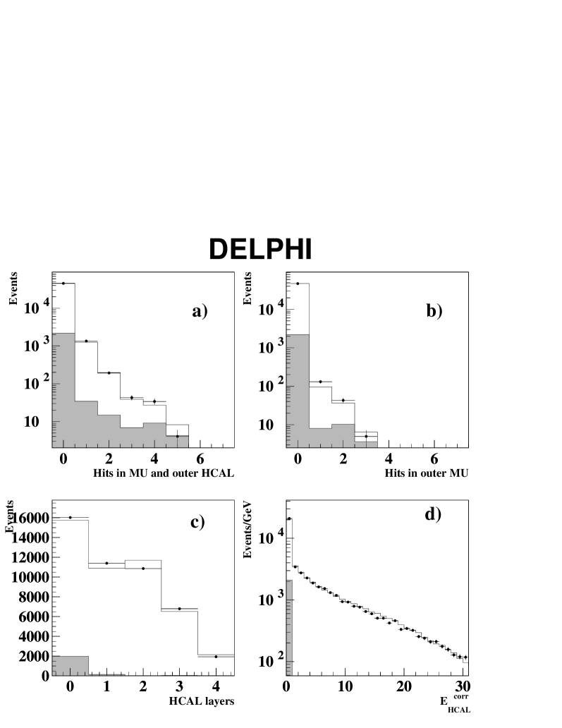
Figure 4: Muon-identification variables for hadron test samples in $\tau$-decays: a) number of muon chamber hits including the outer HCAL layer; b) number of muon chamber hits in the outer muon chambers; c) number of layers in the HCAL; d) corrected deposited energy in the HCAL. Data are shown as dots and simulation after the corrections described in the text, by a solid line. The shaded area represents the non-hadron background.

Figure 5: Distribution of reconstructed invariant mass in GeV/$c^{2}$ (left) and neural-network output (right) reconstructed with the single-cluster algorithm for showers from the tight $\rho$ sample at different energies and for showers from the isolated-$\gamma$ sample from $\mu^{+}\mu^{-}\gamma$. Data are shown as dots and simulation by a solid line.

Figure 7: Distribution for candidate photon clusters for the inclusive sample of $\tau$-decays: Number of HPC layers hit (a); fraction of energy deposited in the four innermost layers (b). Data are shown as dots and simulation by a solid line. The dashed line shows in arbitrary normalization the distributions for showers produced from charged hadrons.

Figure 9: Energy distributions of identified photons in the HPC for $\tau$-decays containing 1, 2, 3 or 4 such clusters. The figures on the left represent the most energetic cluster in the decay and those on the right the least energetic. Data are shown as dots and simulation by a solid line.

Figure 10: Distribution of opening angle between different types of showers: a) a neutral shower fulfilling the $\gamma$ identification with a shower associated to a track b) two neutral showers fulfilling the $\gamma$ identification, c) a neutral shower failing the $\gamma$ identification with a shower associated to a track c) a neutral shower fulfilling the $\gamma$ identification with another one failing it. Data are shown as dots and simulation by a solid line.

Figure 11: The fraction events, as a function of $\pi^{0}$ energy with: (top) 0,1,2, or more than 2, photons reconstructed; (bottom) a reconstructed conversion before or after the TPC, for a sample of simulated non-radiative $\rho$-decays.

Figure 12: Distribution of $\gamma$$\gamma$ invariant mass for $\pi^{0}$ candidates for two neutral showers (top), neutral shower-converted photon (middle) and charged-neutral shower (bottom) . Data are shown as dots and simulation by a solid line.

Figure 13: Total $\pi^{0}$ reconstruction efficiency (top) and probability to reconstruct a $\pi^{0}$ in any of the classes described in the text (bottom) as a function of the $\pi^{0}$ energy for simulated $\rho$ decays.

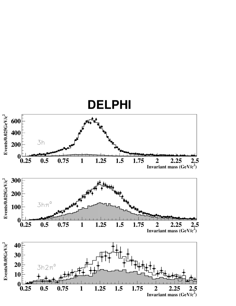
Figure 18: Invariant-mass distributions for the three-prong decays selected with the neural network. Data are shown as dots, simulation by a solid line. The shaded area shows the background prediction from simulation.

References

- [1] M.L. Perl et al., Phys. Rev. Lett. 35 (1975) 1489.
- [2] Y.-S. Tsai, Phys. Rev. D4 (1971) 2821; erratum Phys. Rev. D13 (1976) 771.
- [3] DELPHI Collab., P. Abreu et al., Zeit. Phys. C55 (1992) 555.
-
[4]
ALEPH Collab., D. Buskulic et al., Zeit. Phys., C70 (1996) 579
L3 Collab., M. Acciarri et al.,Phys. Lett. B345 (1995) 93.
OPAL Collab., K. Ackerstaff et al.,Eur. Phys. J. C8 (1999) 183
OPAL Collab., K. Ackerstaff et al.,Eur. Phys. J. C4 (1998) 193
OPAL Collab., R. Akers et al., Zeit. Phys., C68 (1995) 555 - [5] DELPHI Collab., P. Aarnio et al., Nucl. Instr. and Meth. A303 (1991) 233.
- [6] DELPHI Collab., P. Abreu et al., Nucl. Instr. and Meth. A378 (1996) 57.
- [7] S. Jadach, B.F.L. Ward and Z. Was, Comp. Phys. Comm. 79 (1994) 503.
- [8] J.E. Campagne and R. Zitoun, Zeit. Phys. C43 (1989) 469.
- [9] F.A. Berends, R. Kleiss and W. Hollik, Nucl. Phys. B304 (1988) 712.
- [10] S. Jadach, W. Placzek and B.F.L. Ward, Phys. Lett. B390 (1997) 298.
- [11] T. Sjöstrand, Comp. Phys. Comm. 82 (1994) 74.
-
[12]
F.A. Berends, P.H. Daverveldt and R. Kleiss,
Phys. Lett. B148 (1984) 489;
Comp. Phys. Comm. 40 (1986) 271. - [13] T. Alderweireld et al., CERN Report CERN-2000-009 (2000) 219.
- [14] S. Jadach et al., Comp. Phys. Comm. 76 (1993) 361.
- [15] DELPHI Collab., P. Abreu et al., Eur. Phys. J. C10 (1999) 201.
- [16] DELPHI Collab., P. Abreu et al., Eur. Phys. J. C20 (2001) 617.
- [17] DELPHI Collab., W. Adam et al., Zeit. Phys. C69 (1996) 561.
- [18] Particle Data Group, K. Hagiwara et al., Phys. Rev. D 66 (2002) 010001
- [19] R. Odorico, Comp. Phys. Comm., 96 (1996) 314.
- [20] DELPHI Collab., P. Abreu et al., Phys. Lett. B426 (1998) 411.
- [21] CLEO Collab., K.W. Edwards et al., Phys. Rev. D61 (2000) 072003.
- [22] DELPHI Collab., P. Abreu et al., Eur. Phys. J. C14 (2000) 585.