Heavy Flavours and CP violation

Abstract:

Recent results on Heavy Flavours and CP violation are presented. After a short introduction a taste of K and D results is given. In a third part results on $|V_{td}|$ and $|V_{ts}|$ are summaryzed including $B\kern 1.79993pt\overline{\kern-1.79993ptB}{}$ mixing results and $B_{d}$ radiative decays. A summary of $|V_{cb}|$ and $|V_{ub}|$ measurements is presented in the fourth part. In the next section CP violation measurements in the $B_{d}$ sector are shown. Finally in the last part the overall status of the determination of the CKM matrix is presented both in the context of the Standard Model and in the context of New Physics.

PoS(HEP2005)410

1 Introduction

Accurate studies of charm and beauty hadrons allow to test the Standard Model in the fermionic sector in particular for tests of the CP violation mechanism in the B sector, provide information on non perturbative QCD parameters which can be compared with lattice QCD calculations and open a window for searching for New Physics through loop processes.

In the Standard Model, weak interactions among quarks are encoded in a 3 $\times$ 3 unitary matrix: the CKM matrix. The existence of this matrix conveys the fact that quarks, in weak interactions, act as linear combinations of mass eigenstates [1, 2]. The general form of the CKM matrix is :

$$V=\left(\begin{array}[]{ccc}V_{ud}~{}~{}V_{us}~{}~{}V_{ub}\\ V_{cd}~{}~{}V_{cs}~{}~{}V_{cb}\\ V_{td}~{}~{}V_{ts}~{}~{}V_{tb}\end{array}\right).$$ (1)

The CKM matrix can be parametrised in terms of four free parameters which are measured in several physics processes. In the Wolfenstein approximation, these parameters are named: $\lambda$, A, $\rho$ and $\eta$ and the CKM matrix can be parametrised as :

$$\begin{array}[]{cccc}V_{CKM}=&\left(\begin{array}[]{ccc}1-\frac{\lambda^{2}}{2}&\lambda&A\lambda^{3}(\rho-i\eta)\\ -\lambda&1-\frac{\lambda^{2}}{2}&A\lambda^{2}\\ A\lambda^{3}(1-\overline{\rho}-i\overline{\eta})&-A\lambda^{2}&1\end{array}\right)&+O(\lambda^{4}).\end{array}$$ (2)

with $\overline{\rho}=\rho(1-\frac{\lambda^{2}}{2})~{}~{}~{};~{}~{}~{}\overline{\eta}=\eta(1-\frac{\lambda^{2}}{2})$[3]. It is worthwhile noting that the expressions for $|V_{us}|$ and $|V_{cb}|$ are valid up to order $\lambda^{7}$ and $\lambda^{8}$ respectively. CP violation is accommodated in the CKM matrix with a single parameter and its existence is related to $\overline{\eta}\neq 0$.
From the unitarity of the CKM matrix ($VV^{{\dagger}}=V^{{\dagger}}V=1$), non diagonal elements of the matrix products, corresponding to six equations relating its elements, can be written. In particular, in transitions involving $b$ quarks, the scalar product of the third column with the complex conjugate of the first row must vanish:

$$V_{ud}^{\ast}V_{ub}~{}+~{}V_{cd}^{\ast}V_{cb}~{}+~{}V_{td}^{\ast}V_{tb}~{}=~{}0$$ (3)

This equation can be visualised as a triangle in the ($\overline{\rho},\overline{\eta}$) plane (Figure 1).

Figure 1: The Unitarity Triangle.

The angles $\beta$ and $\gamma$ of the unitarity triangle are related directly to the complex phases of the CKM-elements $V_{td}$ and $V_{ub}$ respectively, through

$$V_{td}=|V_{td}|e^{-i\beta},\qquad V_{ub}=|V_{ub}|e^{-i\gamma}.$$ (4)

Each of the angles is the relative phase of two adjacent sides :

$$\beta= arg(\frac{V_{td}V_{tb}^{*}}{V_{cd}V_{cb}^{*}})$$ (5)

$$\gamma= arg(\frac{V_{ud}V_{ub}^{*}}{V_{cd}V_{cb}^{*}})$$ (6)

The angle $\alpha$ can be obtained through the relation $\alpha+\beta+\gamma=180^{\circ}$ expressing the unitarity of the CKM-matrix .

The triangle shown in Figure 1 -which depends on two parameters ($\overline{\rho},~{}\overline{\eta}$)-, plus $|V_{us}|$ and $|V_{cb}|$ give the full description of the CKM matrix.

The Standard Model, with three families of quarks and leptons, predicts that all measurements have to be consistent with the point A($\overline{\rho},~{}\overline{\eta}$). Extensions of the Standard Model can provide different predictions for the position of the apex of the triangle, given by the $\overline{\rho}$ and $\overline{\eta}$ coordinates.
The most precise determination of these parameters is obtained using B decays, $B^{0}$ - $\kern 1.79993pt\overline{\kern-1.79993ptB}{}^{0}$ oscillations and CP asymmetry in the B and in the K sectors. Many additional measurements of B meson properties (mass, branching fractions, lifetimes…) are necessary to constrain the Heavy Quark theories [Operator Product Expansion (OPE) /Heavy Quark Effective Theory (HQET) /Lattice QCD (LQCD)] to allow for precise extraction of the CKM parameters.

In principle Heavy Flavours deals with strange, charm and beauty hadrons. Due to lack of time, only a taste of K and D physics results will be given, emphasis will be put on B physics. Apologies to those whose work I did not have time to mention.

2 A taste of K and D results

In this section emphasis will be given to new results related to CP violation.

2.1 Some K decays

The very rare decays $K\rightarrow\pi\nu{\overline{\nu}}$ (with branching fractions of the order of $10^{-10}$ to $10^{-11}$) provide clean constraints on the CKM parameters but they are experimentally very challenging. Only, the charged decay $K^{\pm}\rightarrow\pi^{\pm}\nu{\overline{\nu}}$ has been observed [4], for the corresponding neutral one ($K^{0}_{\scriptscriptstyle L}\rightarrow\pi^{0}\nu{\overline{\nu}}$) only upper limits are available. The Feynmann diagram for the decay and the selection plot for $K^{\pm}\rightarrow\pi^{\pm}\nu{\overline{\nu}}$ are shown on Figure 2. Other modes such as $K\rightarrow\pi^{0}\ell^{+}\ell^{-}$ have been searched for, but only upper limits are available at present. The current status is summarised in Table 1.

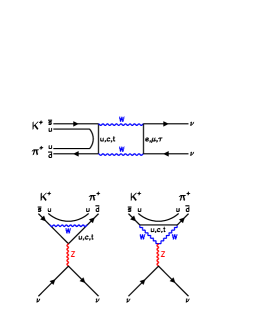
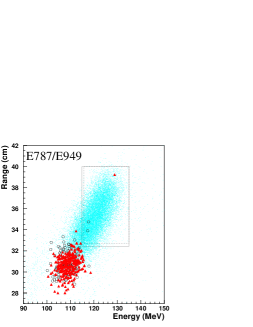
Figure 2: Left : the Feynman diagrams corresponding to the $K\rightarrow\pi\nu{\overline{\nu}}$ decay. Right : final plot of the E787/E949 experiments. The empty circles represent E787 data and the triangles E949 data. The dots are signal Monte Carlo events. The solid (dashed) line box represents the signal region for E949 (E747).

Mode	SM prediction	Exp. results	CKM parameter
$K^{\pm}\rightarrow\pi^{\pm}\nu{\overline{\nu}}$	$(8.0\pm 1.0)\ 10^{-11}$	$1.47^{+1.30}_{-0.89}\ 10^{-10}$ [4] E787/E949	$||V_{ts}|^{*}|V_{td}||$
$K^{0}_{\scriptscriptstyle L}\rightarrow\pi^{0}\nu{\overline{\nu}}$	$(3.0\pm 0.6)\ 10^{-11}$	$<2.9\ 10^{-7}$ [5] E391a	Im$(|V_{ts}|^{*}|V_{td}|)\sim\eta$
$K^{0}_{\scriptscriptstyle L}\rightarrow\pi^{0}e^{+}e^{-}$	$(3.7\pm 1.1)\ 10^{-11}$	$<2.8\ 10^{-10}$ [6] KTeV	Im$(|V_{ts}|^{*}|V_{td}|)\sim\eta$
$K^{0}_{\scriptscriptstyle L}\rightarrow\pi^{0}\mu^{+}\mu^{-}$	$(1.5\pm 0.5)\ 10^{-11}$	$<3.8\ 10^{-10}$ [7] KTeV	Im$(|V_{ts}|^{*}|V_{td}|)\sim\eta$

Table 1: Summary of the current status for $K\rightarrow\pi\nu{\overline{\nu}}$ and $K\rightarrow\pi^{0}\ell^{+}\ell^{-}$ decays. For the $K\rightarrow\pi^{0}\ell^{+}\ell^{-}$ decay modes, improvements on the theoretical uncertainty are expected. New Physics effects can be different for the electron and the muon channels. The upper limits are given at 90 % CL.

The branching fraction of the CP violating decay $K^{0}_{\scriptscriptstyle S}\rightarrow\pi^{0}\pi^{0}\pi^{0}$ is expected to be of the order of $1.9\ 10^{-9}$ in the Standard Model. The best limits obtained are summarised in Table 2.

Experiment	Method	limit at 90 % CL
NA48 [8]	$K^{0}$ beam : interference	$<7.4\ 10^{-7}$
KLOE [9]	direct search (tagged $K^{0}_{\scriptscriptstyle S}$ from $\phi$ decay)	$<1.2\ 10^{-7}$

Table 2: Summary of the current status for the search of the CP violating decay $K^{0}_{\scriptscriptstyle S}\rightarrow\pi^{0}\pi^{0}\pi^{0}$.

Direct CP violation in the decay $K^{\pm}\rightarrow\pi^{\pm}\pi^{\pm}\pi^{\mp}$ has been searched for using asymmetry in the comparison of the $K^{+}$ and the $K^{-}$ Dalitz plot. Standard Model expectations vary between $10^{-6}$ and few $10^{-5}$, the NA48/2 collaboration has obtained a preliminary result consistent with no CP violation : $(0.5\pm 3.8)\ 10^{-4}$ [10], improving by one order of magnitude previous results.

2.2 Leptonic and semi-leptonic charm decays

The leptonic decay $D\rightarrow\ell\nu$ width depends on few parameters :

$$\Gamma(D\rightarrow\ell\nu)=\frac{1}{8\pi}G_{F}^{2}f_{D}^{2}m_{\ell}^{2}M_{D}\left(1-\frac{m_{\ell}^{2}}{M_{D}^{2}}\right)^{2}|V_{cd}|^{2}$$ (7)

Since the CKM matrix element $|V_{cd}|$ is precisely known the measurement of this partial width is equivalent to a measurement of $f_{D}$ the pseudo-scalar constant which translate the quarks wave functions overlap. It can be compared with theoretical predictions from non perturbative QCD calculations. The latest result has been obtained by the CLEO-c experiment which runs at the $\Psi^{{}^{\prime\prime}}(3770)$ resonance decaying into a correlated $D\bar{D}$ pair. One charged $D$ is fully reconstructed (the tagging $D$), a muon of charge opposite to the tagging D charge is searched for in the remaining tracks, requiring no additional activity in the calorimeters. The discriminating variable is the missing mass squared which should be compatible with 0 in case of signal (Figure 3). Using an integrated luminosity of 281 $\mbox{\,pb}^{-1}$, a branching fraction of $(4.45\pm 0.67^{+0.29}_{-0.36})\ 10^{-4}$ is obtained [11]. It can be translated into : $f_{D}=(223\pm 16^{+7}_{-9})$ MeV, this result is compared with previous results and the latest LQCD computation (Figure 3).

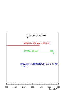
Figure 3: Left : the missing mass squared variable for the events passing all the selection cuts. The insert is a zoom on the signal region, the arrows indicate the cuts. There are 50 events in the signal region with a background of $2.93\pm 0.50$ events. Right : comparison of the CLEO-c result for $f_{D}$ with previous experimental values and LQCD computation.

Using the tagging D technique, various semi-leptonic decays of both $D^{\pm}$ and $D^{0}$ have been reconstructed by CLEO-c. They are compared with the present PDG values in Table 3.

$D^{+}\rightarrow$	CLEO-c (BF %)	PDG (BF%)	$D^{0}\rightarrow$	CLEO-c (BF %)	PDG (BF%)
$\kern 1.99997pt\overline{\kern-1.99997ptK}{}^{0}e^{+}\nu_{e}$	$8.71\pm 0.38\pm 0.37$	$6.7\pm 0.9$	$K^{-}e^{+}\nu_{e}$	$3.44\pm 0.10\pm 0.10$	$3.58\pm 0.18$
$\pi^{0}e^{+}\nu_{e}$	$0.44\pm 0.06\pm 0.03$	$0.31\pm 0.15$	$\pi^{-}e^{+}\nu_{e}$	$0.262\pm 0.025\pm 0.008$	$0.36\pm 0.06$
$\kern 1.99997pt\overline{\kern-1.99997ptK}{}^{*0}e^{+}\nu_{e}$	$5.56\pm 0.27\pm 0.23$	$5.5\pm 0.7$	$K^{*-}e^{+}\nu_{e}$	$2.16\pm 0.15\pm 0.08$	$\--$
$\rho^{0}e^{+}\nu_{e}$	$0.21\pm 0.04\pm 0.01$	$0.25\pm 0.10$	$\rho^{-}e^{+}\nu_{e}$	$0.194\pm 0.039\pm 0.013$	$\--$
$\omega e^{+}\nu_{e}$	$0.16^{+0.07}_{-0.06}\pm 0.01$	$\--$

Table 3: Summary of the semileptonic decays modes branching fractions as measured by CLEO-c.

Since $|V_{cd}|$ is very well known, these measurements can be used to extract the D form factors, which can, in turn, be used in several ways as for example :

• The form factor of the mode $D\rightarrow K\ell\nu$ provide validation of LQCD computations.

• The form factors from $D\rightarrow\rho/\pi\ell\nu$ modes can be related to the B form factor for similar charmless decay modes, which helps reducing the theoretical uncertainty on the $|V_{ub}|$ extraction.

3 $|V_{td}|$ and $|V_{ts}|$ measurements

The CKM matrix elements $|V_{td}|$ and $|V_{ts}|$ can be measured in the B physics sector through processes described by loop or box diagrams involving top quark contributions. The presence of such diagrams allows also to search for New Physics since new particles may appear as well in the loops.

3.1 $B\kern 1.79993pt\overline{\kern-1.79993ptB}{}$ mixing

The probability that a meson $B^{0}$ produced at time $t=0$ transforms into a $\kern 1.79993pt\overline{\kern-1.79993ptB}{}^{0}$ (or stays as a $B^{0}$) at time $t$ is given by :

$$Prob(B^{0}(t=0)\rightarrow B^{0}(t)(\kern 1.79993pt\overline{\kern-1.79993ptB}{}^{0}(t)))=\frac{1}{2}e^{-\Gamma t}(1+(-)cos\Delta mt)$$ (8)

In the Standard Model, $B^{0}{\kern-1.60004pt\kern 1.79993pt\overline{\kern-1.79993ptB}{}^{0}}$ oscillations occur through a second-order process -a box diagram- with a loop that contains W and up-type quarks. The box diagram with the exchange of a $top$ quark gives the dominant contribution. The oscillation probability is given in eq. (8) and the time oscillation frequency, which can be related to the mass difference between the light and heavy mass eigenstates of the $B_{d}$ or $B_{s}$ meson system, is expressed in the SM, as :

$${\rm\Delta}m_{q}\ =\frac{G_{F}^{2}}{6\pi^{2}}|V_{tb}|^{2}|V_{tq}|^{2}M_{W}^{2}M_{B_{q}}\eta_{b}S(x_{t})f_{B_{q}}^{2}\hat{B}_{B_{q}}$$ (9)

where $S(x_{t})$ is the Inami-Lim function [12] and $x_{t}=m_{t}^{2}/M^{2}_{W}$, $m_{t}$ is the $\overline{MS}$ top quark mass, and $\eta_{b}$ is the perturbative QCD short-distance NLO correction. The remaining factor, $f_{B_{q}}^{2}\hat{B}_{B_{q}}$, encodes the information of non-perturbative QCD. Apart for the CKM matrix elements, the most uncertain parameter in this expression is $f_{B_{q}}\sqrt{\hat{B}_{B_{q}}}$.

Experimentally the parameter ${\rm\Delta}m_{d}$ is now very precisely measured [13] : ${\rm\Delta}m_{d}=0.509\pm 0.004\mbox{\,ps}^{-1}$ ; the accuracy of the order of 1 %, is dominated by the B factories results.

Due to the relative size of the CKM matrix elements the $B_{s}$ meson is expected to oscillate much faster than the $B_{d}$ meson and has not been measured yet. The method used to set a limit on $\Delta{m}_{s}$ consists in modifying Equation 8 in the following way [14]:

$$1\pm\cos{({\rm\Delta}m_{s}t)}\rightarrow 1\pm{\cal A}\cos{({\rm\Delta}m_{s}t)}.$$ (10)

${\cal A}$ and its error, $\sigma_{{\cal A}}$, are measured at fixed values of ${\rm\Delta}m_{s}$, instead of ${\rm\Delta}m_{s}$ itself. In case of a clear oscillation signal, at a given frequency, the amplitude should be compatible with ${\cal A}=1$ at this frequency. With this method it is easy to set a limit. The values of ${\rm\Delta}m_{s}$ excluded at 95% C.L. are those satisfying the condition ${\cal A}({\rm\Delta}m_{s})+1.645\sigma_{{\cal A}({\rm\Delta}m_{s})}<1$. With this method, it is easy also to combine results from different experiments and to treat systematic uncertainties in the usual way since, for each value of ${\rm\Delta}m_{s}$, a value for $\cal A$ with a Gaussian error $\sigma_{\cal A}$, is measured. Furthermore, the sensitivity of a given analysis can be defined as the value of ${\rm\Delta}m_{s}$ corresponding to 1.645 $\sigma_{\cal A}({\rm\Delta}m_{s})=1$ (using ${\cal A}({\rm\Delta}m_{s})=0$), namely supposing that the “true” value of ${\rm\Delta}m_{s}$ is well above the measurable value. Combining, with this amplitude method, the LEP and Tevatron results [13] one gets : ${\rm\Delta}m_{s}>14.4\ \mbox{\,ps}^{-1}$ at 95 % C. L. with a sensitivity ${\rm\Delta}m_{s}=18.8~{}\mbox{\,ps}^{-1}.$ The averaged amplitudes are shown in Figure 4.

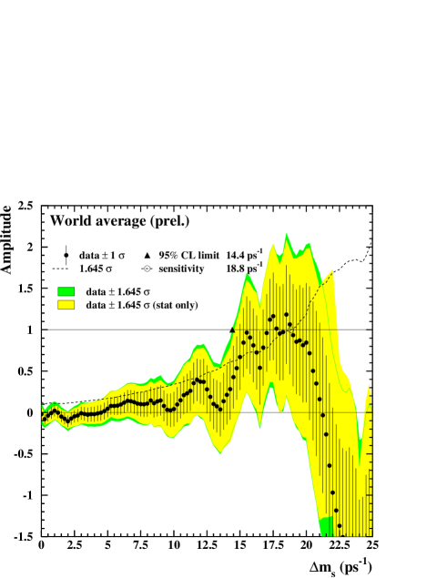
Figure 4: The plot [13] gives combined $\Delta{m}_{s}$ results from LEP/SLD/CDF analyses shown as an amplitude versus ${\rm\Delta}m_{s}$ plot. The points with error bars are the data; the lines show the 95% C.L. curves (darker regions correspond to the inclusion of systematics). The dotted curve corresponds to the sensitivity.

The only two running experiments which can study $B_{s}{\kern-1.60004pt\kern 1.79993pt\overline{\kern-1.79993ptB}{}_{s}}$ mixing today are D0 and CDF at Tevatron. Their current limits are summarised in Table 4.

Experiment	Sensitivity	95 % CL limit
CDF 355 $\mbox{\,pb}^{-1}$ ($D_{s}\ell\nu$ and $D_{s}\pi$) [15]	8.4 $\mbox{\,ps}^{-1}$	7.9 $\mbox{\,ps}^{-1}$
D0 610 $\mbox{\,pb}^{-1}$ ($D_{s}\ell\nu$ ) [16]	9.5 $\mbox{\,ps}^{-1}$	7.3 $\mbox{\,ps}^{-1}$

Table 4: Summary of the Tevatron results on ${\rm\Delta}m_{s}$.

The experiments CDF and D0 have performed prospect studies, taking into account their current performances and foreseen experimental improvements [17]. Each experiment, with an integrated luminosity of about 4 $\mbox{\,fb}^{-1}$ (about 4 times the current one), should be able to push the ${\rm\Delta}m_{s}$ limit up to about 20 $\mbox{\,ps}^{-1}$.

3.2 Radiative B decays

Radiative B decays occur via penguins diagrams. Due to the difference in magnitude between the CKM matrix element $|V_{ts}|$ and $|V_{td}|$, the $b\rightarrow s\gamma$ type decays are much more copiously produced than the $b\rightarrow d\gamma$ type decays. The study of the inclusive $\gamma$ energy spectrum in $b\rightarrow s\gamma$ type decays gives information on the $b$ quark motion inside the $B$ meson and helps reducing the theoretical uncertainties in the $|V_{cb}|$ and $|V_{ub}|$ extraction using semi-leptonic $B$ decays. Two main types of analyses for the $b\rightarrow s\gamma$ modes are performed [18] : fully inclusive ones where the photon energy spectrum is measured without reconstructing the $X_{s}$ system, and the backgrounds are suppressed using information from the rest of the event. The second method, the semi-inclusive one, uses a sum of exclusive final states in which possible $X_{s}$ system (about 55% of the modes are reconstructed) are combined with the photon and kinematic constraints of the $\Upsilon(4S)$ reconstruction are used to suppress the background. The ratio of the $b\rightarrow s\gamma$ and $b\rightarrow d\gamma$ branching fractions could, in principle, provide information similar to the $B^{0}{\kern-1.60004pt\kern 1.79993pt\overline{\kern-1.79993ptB}{}^{0}}$ mixing analysis. The theoretical uncertainties are smaller for the inclusive measurements, but this cannot be achieved for the $b\rightarrow d\gamma$ decay due to the huge background. Only exclusive reconstruction can be performed for the time being. In that case the theoretical uncertainties are more difficult to control. The first observation at $5.5\sigma$ for these $b\rightarrow d\gamma$ type decays has been shown by BELLE. The results are summarised in Table 5.

Experiment	BF($B\rightarrow\rho/\omega\gamma$)
BABAR (211 $10^{6}$ $B\kern 1.79993pt\overline{\kern-1.79993ptB}{}$ pairs)  [19]	$<1.2\ 10^{-6}$ at 90 % CL
BELLE (386 $10^{6}$ $B\kern 1.79993pt\overline{\kern-1.79993ptB}{}$ pairs) [20]	$(1.34^{+0.34\ +0.14}_{-0.31\ -0.10})10^{-6}$

Table 5: Summary of the BABAR and BELLE results for the $b\to d\gamma$ analyses.

The selection plots for the BELLE analysis are shown in Figure 5.

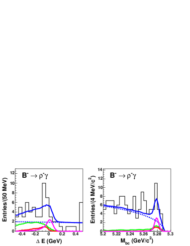
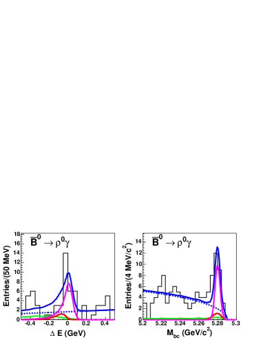
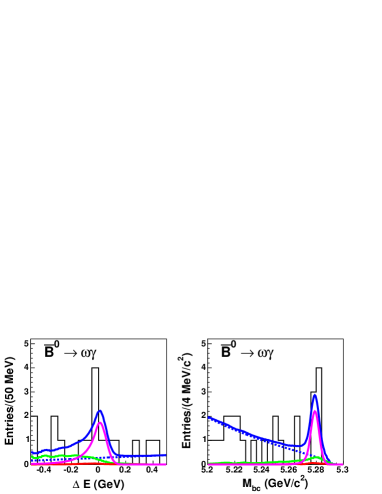
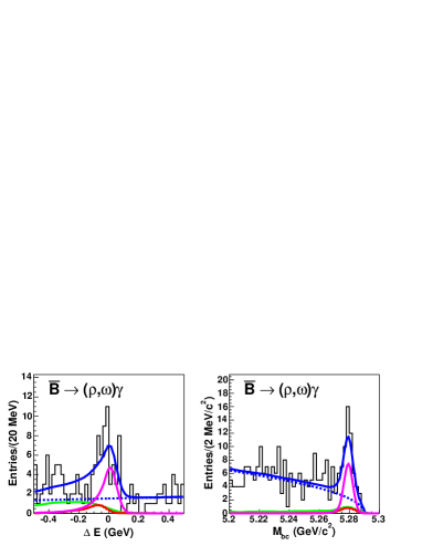
Figure 5: Projections of the fit results [20] on the B mass and $\Delta E$ for the individual modes. Lines represent the signal (magenta), continuum (blue-dashed), $B\rightarrow K^{*}\gamma$ (red), other $B$ decays background components (green) and the total fit result (blue-solid). The $\overline{B}$ symbol represent the sum for neutral and charged $B$ mesons decays.

4 $|V_{cb}|$ and $|V_{ub}|$ measurements

4.1 Semileptonic B decays

The weak semi-leptonic decay of a free quark can be simply expressed :

$$\Gamma_{0}\equiv\Gamma(b\rightarrow q\ell{\overline{\nu}})=\frac{G_{F}^{2}|V_{tq}|^{2}}{192\pi^{3}}m_{b}^{5}.$$ (11)

However at the hadron level the expression gets more complicated due to the hadronization process [21]:

$$\frac{\partial^{3}\Gamma}{\partial E_{\ell}\partial q^{2}\partial m_{X}}=\Gamma_{0}\times f(E_{\ell},q^{2},m_{X})\times\left(1+\sum_{n}C_{n}\left(\frac{\Lambda_{QCD}}{m_{b}}\right)^{n}\right)$$ (12)

The term in parenthesis contains the perturbative and non-perturbative corrections to the semi-leptonic width. In exclusive decays it depends on QCD form factors which can be for example obtained from LQCD computations. In inclusive decays one uses Heavy Quarks symmetry and the OPE machinery. The OPE parameters can be obtained from data using the spectra and moments from $b\rightarrow s\gamma$ and $b\rightarrow c\ell{\overline{\nu}}$ distributions. In principle it works both for $b\rightarrow c\ell{\overline{\nu}}$ and $b\rightarrow u\ell{\overline{\nu}}$ decays, however because of the very different values of the CKM matrix element one has to deal with $\Gamma(b\rightarrow u\ell{\overline{\nu}})/\Gamma(b\rightarrow c\ell{\overline{\nu}})\sim 50$. Kinematical cuts have to be applied to reject this huge background, the measurements of the partial branching fractions will be performed in restricted phase space regions. As a consequence, the theoretical uncertainties will be more difficult to evaluate.

4.1.1 Extract of $|V_{ub}|$ using inclusive semi-leptonic decays

By using kinematical and topological variables, it is possible to select samples enriched in $b\rightarrow u\ell^{-}{\overline{\nu}}$ transitions. There are, schematically, three main regions in the semi-leptonic decay phase space to be considered : the lepton energy end-point region where $E_{\ell}>\frac{M^{2}_{B}-M^{2}_{D}}{2M_{B}}$ (which was at the origin for the first evidence of $b\rightarrow u$ transitions), the second region is the low hadronic mass region: $M_{X}<M_{D}$ and the last one is the high $q^{2}$ region: $M^{2}_{\ell\nu}=q^{2}>(M_{B}-M_{D})^{2}$ in which the background from $b\rightarrow c\ell^{-}\overline{\nu_{\ell}}$ decays is small. In addition, in some cases one reconstructs (tags) the other B in order to improve the purity of the sample and to add additional kinematical constraints. A summary of the various analyses [22] is given in Table 6 and the HFAG [13] average is shown on the right plot of Figure 6.

Method	Signal/Background	Main points	$|V_{ub}|$ $\times 10^{-3}$
Untagged	0.05 $\rightarrow$ 0.2	High statistics	$4.23\pm 0.27_{\rm{exp}}\pm 0.31_{\rm{theo}}$[23]
$\ell$ spectrum end point		Delicate background	$4.82\pm 0.45_{\rm{exp}}\pm 0.31_{\rm{theo}}$[24]
$E_{\ell}>1.9GeV$		subtraction
Untagged	$\sim 0.5$	High statistics	$4.06\pm 0.27_{\rm{exp}}\pm 0.36_{\rm{theo}}$[25]
$\nu$ reconstruction		Lower syst. on SF
Uses $M_{X}$		Delicate background
Tagged	$\sim 2$	Low background	$4.76\pm 0.34_{\rm{exp}}\pm 0.32_{\rm{theo}}$[26]
$M_{X}$ versus $q^{2}$ analyses		Small syst. on SF	$4.08\pm 0.27_{\rm{exp}}\pm 0.25_{\rm{theo}}$[27]
		Small statistics

Table 6: Summary of the inclusive analyses for the $|V_{ub}|$ measurement.

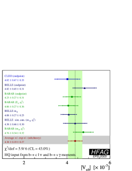
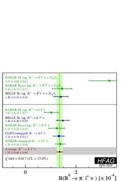
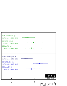
Figure 6: Left plot : summary of the $|V_{ub}|$ values obtained from inclusive analyses. Middle plot : summary of the $B\rightarrow\pi\ell{\overline{\nu}}$ branching fraction measurements. Right plot : the $|V_{ub}|$ values for different FF computations.

4.1.2 Extract of $|V_{ub}|$ using exclusive semi-leptonic decays

The second method to determine $|V_{ub}|$ consists in the reconstruction of charmless semileptonic B decays: $B\rightarrow\pi(\rho)\ell{\overline{\nu}}$.
The probability that the final state quarks form a given meson is described by form factors and, to extract $|V_{ub}|$ from actual measurements, the main problem rests in the determination of these hadronic form factors. Several theoretical approaches are used to compute these hadronic form factors. Experimentally one starts to be able to extract the signal rates in three independent regions of $q^{2}$. In this way it is possible to discriminate between models. An example is given in Figure 7 which shows that the ISGW II model is only marginally compatible with the data. This approach could be used, in future, to reduce the importance of theoretical errors, considering that the ISGW  II gave, at present, the further apart $|V_{ub}|$ determination.

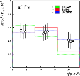
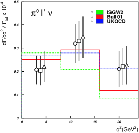
Figure 7: Extracted $q^{2}$ distribution for the $B\rightarrow\pi\ell{\overline{\nu}}$ modes [28]. Data points are shown for different Form Factor models used to estimate the detection efficiency. Lines are for the best fit of the Form factors shapes to the obtained $q^{2}$ distribution.

The summary of the $B\rightarrow\pi\ell{\overline{\nu}}$ branching fraction measurements [13] is given in the middle plot of Figure 6 and can be translated into a $|V_{ub}|$ measurement. There exist several theoretical computations of the Form Factors leading to different $|V_{ub}|$ values, as can be seen from the right plot of Figure 6. Despite this precise measurement (of the order of 8 %) the uncertainty on $|V_{ub}|$ is still of the order of 20%, dominated by theoretical uncertainty.

The determination of $|V_{ub}|$ from inclusive and exclusive semi-leptonic B decays are in agreement. The inclusive determination is the most precise one.

4.1.3 $|V_{cb}|$ determination

No new experimental results on $|V_{cb}|$ extraction were presented at this conference. The average for the inclusive determination is equal to $(41.58\pm 0.45\pm 0.58_{\Gamma_{SL}})\ 10^{-3}$ [29] and the average for the exclusive method is : $|V_{cb}|=(41.3\pm 1.0\pm 1.8)\ 10^{-3}$ [13]. The two determinations are in good agreement.

4.2 $B\rightarrow\tau\nu$

The partial width of the $B\rightarrow\tau{\overline{\nu}}$ decay depends on few parameters :

$$\Gamma(B\rightarrow\tau\nu)=\frac{1}{8\pi}G_{F}^{2}f_{B}^{2}m_{\tau}^{2}M_{B}\left(1-\frac{m_{\tau}^{2}}{M_{D}^{2}}\right)^{2}|V_{ub}|^{2}$$ (13)

A measurement of this partial width is thus equivalent, in the Standard Model, to a measurement of $f_{B}|V_{ub}|$. Using the value of $|V_{ub}|$ from semi-leptonic decays and assuming the Standard Model, this could be translated into a $f_{B}$ measurement which could be compared with LQCD computations. In case of New Physics , there could be additional diagram with a charged Higgs, such an analysis provides constraints on New Physics. Experimentally, in order to reduce the very large background, one B is fully reconstructed and the decay of interest is searched in the rest of the event. It is characterised by the presence of two neutrinos. The current results are summarised in Table 7. The present limits are getting close to the Standard Model expected value ($8.2^{+1.7}_{-1.3})\ 10^{-5}$ predicted by [30],[31].

Experiment	BF($B\rightarrow\tau\nu$) limit at 90 % CL )
BABAR (232 $10^{6}$ $B\kern 1.79993pt\overline{\kern-1.79993ptB}{}$ pairs)) [32]	$2.6\ 10^{-4}$
BELLE (275 $10^{6}$ $B\kern 1.79993pt\overline{\kern-1.79993ptB}{}$ pairs) [33]	$1.8\ 10^{-4}$

Table 7: Summary of BF($B\rightarrow\tau\nu$) 90 % CL limits.

5 CP violation in B decays

Following [34], CP violation can be categorised into three types :

CP violation in the decay

: it is the case where ${\cal A}(B\rightarrow f)\neq{\cal A}(\overline{B}\rightarrow\overline{f})$. There should exist two amplitudes with different weak and strong phases to reach the final state $f$. This type of CP violation can be seen both in charged and neutral $B$ decays.

CP violation in the mixing

: it is the case where ${\cal A}(B^{0}\rightarrow\kern 1.79993pt\overline{\kern-1.79993ptB}{}^{0})\neq{\cal A}(\kern 1.79993pt\overline{\kern-1.79993ptB}{}^{0}\rightarrow B^{0})$. This type of CP violation is due to the fact that the CP eigenstates are not the mass eigenstates.

CP violation in the interference between mixing and decay

: it is due to the interference between a decay without mixing, $B^{0}\rightarrow f$ and a decay with mixing $B^{0}\rightarrow\kern 1.79993pt\overline{\kern-1.79993ptB}{}^{0}\rightarrow f$ (such an effect occurs only in decays where $f$ is common to $B^{0}$ and $\kern 1.79993pt\overline{\kern-1.79993ptB}{}^{0}$). The most famous example is ${\cal A}(B^{0}\rightarrow J/\Psi K^{0}_{\scriptscriptstyle S})\neq{\cal A}(\kern 1.79993pt\overline{\kern-1.79993ptB}{}^{0}\rightarrow J/\Psi K^{0}_{\scriptscriptstyle S})$.

CP violation has been first observed in the neutral Kaon system as the effect of CP violation in mixing. This type of CP violation is expected to be small ($10^{-3}$ to $10^{-4}$) in the $B^{0}$ meson system. A large violation is possible in the Standard Model both as direct CP violation and as time-dependent CP violation in the interference between mixing and decay. The time evolution of $B^{0}$, taking into account CP violation can be written as :

$$Prob(B^{0}(t=0)\rightarrow B^{0}(t)(\kern 1.79993pt\overline{\kern-1.79993ptB}{}^{0}(t)))=\frac{1}{4\tau}e^{-t/\tau}(1+(-)C\cos({\rm\Delta}m_{d}t)-(+)S\sin({\rm\Delta}m_{d}t))$$ (14)

The parameter $S$ is non-zero if there is mixing induced CP violation, while a non-zero value for $C$ would indicate direct CP violation.

5.1 $B\rightarrow$ charmonium : $\beta$ or $\phi_{1}$

For this type of decay the dominant penguin contribution has the same weak phase, so no direct CP violation is expected to be seen. The only diagram with a different weak phase is suppressed by a factor $\lambda^{2}$ and by OZI. For these $B^{0}\rightarrow(c\overline{c})K^{0}$ decays one should measure : $C=0$ and $S=\eta\sin\!2\beta$ with ($\eta=+1$ for $K^{0}_{\scriptscriptstyle S}$ and $\eta=-1$ for $K^{0}_{\scriptscriptstyle L}$). The measurements of $\sin\!2\beta$ [35] are summarised in Table 8. The overall average is $\sin\!2\beta=0.685\pm 0.032$ [13], a 5 % precision measurement. This precise value is in good agreement with the predicted one from fits using constraints only from sides of the Unitarity Triangle [30],[31]. This indicates a coherent description of CP violation within the Standard Model and that Standard Model is the dominant source of CP violation in the B meson sector.

Experiment	BABAR (227 $10^{6}$ $B\kern 1.79993pt\overline{\kern-1.79993ptB}{}$ pairs) [36]	BELLE (386 $10^{6}$ $B\kern 1.79993pt\overline{\kern-1.79993ptB}{}$ pairs) [37]
$\sin\!2\beta$ from $c\overline{c}$ $K^{0}_{\scriptscriptstyle S}$	$0.75\pm 0.04_{\rm{stat}}$	$0.668\pm 0.047_{\rm{stat}}$
$\sin\!2\beta$ from $c\overline{c}$ $K^{0}_{\scriptscriptstyle L}$	$0.57\pm 0.09_{\rm{stat}}$	$0.619\pm 0.069_{\rm{stat}}$
All charmonium	$0.722\pm 0.040_{\rm{stat}}\pm 0.023_{\rm{syst}}$	$0.652\pm 0.039_{\rm{stat}}\pm 0.020_{\rm{syst}}$

Table 8: Summary of the $\sin\!2\beta$ measurements.

5.2 $B^{-}\rightarrow D^{(*)0}K^{(*)-}$: $\gamma$ or $\phi_{3}$ , $\beta$ or $\phi_{1}$

Different approaches have been used to measure the angle $\gamma$ (or $\phi_{3}$) of the Unitarity Triangle. They exploit the interference between $b\rightarrow c$ and $b\rightarrow u$ transitions. Practically, this is achieved using decays of type $B^{-}\rightarrow D^{(*)0}K^{(*)-},\overline{D}^{(*)0}K^{(*)-}$ with subsequent decays into final states accessible to both charmed meson and anti-meson. They are classified in three main types :

The GLW method

[38] : the $D^{0}$ meson decays into a CP final state

The ADS method

[39] : the $D^{0}$ meson is reconstructed into the $K\pi$ final state, for the $b\rightarrow c$ (resp. $b\rightarrow u$) transitions the $D^{0}$ decay mode will be the Cabbibo suppressed : $D^{0}\rightarrow K^{+}\pi^{-}$ (resp. Cabbibo allowed : $D^{0}\rightarrow K^{-}\pi^{+}$) modes. In this way the magnitude of the two interfering amplitudes will not be too different.

The GGSZ method

[40] : the $D^{0}$ final state is $K^{0}_{\scriptscriptstyle S}\pi\pi$ which is accessible to both $D^{0}$ and $\kern 1.79993pt\overline{\kern-1.79993ptD}{}^{0}$. This requires analysis of the $D^{0}$ Dalitz plot, it can be seen as a mixture of the two previous ones, depending on the position in the Dalitz plot.

In all cases the involved diagrams are tree diagrams, so all methods should provide measurements of $\gamma$ independent of the possible existence of New Physics. One of the main problem from the experimental point of view, is that the size of the CP asymmetries involved depend on the ratio of the favoured and the $|V_{ub}|$ and colour suppressed decays : $r_{B}^{(*)}=|\frac{{\cal A}(B^{-}\rightarrow\overline{D}^{(*)0}K^{-}}{B^{-}\rightarrow D^{(*)0}K^{(*)-}}|,$ which is, taking into account CKM matrix elements and colour suppression factors, expected to be of the order 0.1. An other experimental aspect is that the effective branching ratio is of the order of $10^{-7}$ in the case of the GLW and ADS methods. The situation is more favourable in the case of the GGSZ technique but this one is complicated by the necessity to model the complex Dalitz plot of the $D^{0}\rightarrow K^{0}_{\scriptscriptstyle S}\pi\pi$ decay. Due to the very limited effective statistics and to the smallness of the $r_{B}$ parameter, the GLW and ADS methods are not yet able to measure $\gamma$ [41]. The results on $\gamma$ are summarised in Table 9. The large difference on the $\gamma$ statistical uncertainty between the BELLE and BABAR experiments cannot be attributed to the different sample sizes. It is rather due to different central values obtained for the various $r_{B}$ by the two experiments.

Exp	Mode	$r_{B}$	$\gamma$
BABAR[42]	$DK$	$0.118\pm 0.079\pm 0.034^{+0.036}_{-0.034}$
(227 $10^{6}$ $B\kern 1.79993pt\overline{\kern-1.79993ptB}{}$ pairs)	$D^{*}K$	$0.169\pm 0.096^{+0.030+0.029}_{-0.028-0.026}$
	$DK^{*}$	$0.05\pm 0.11\pm 0.05$
	Combined		$67\pm 28\pm 13\pm 11^{\circ}$
BELLE[43]	$DK$	$0.21\pm 0.08\pm 0.03\pm 0.04$
(275 $10^{6}$ $B\kern 1.79993pt\overline{\kern-1.79993ptB}{}$ pairs)	$D^{*}K$	$0.12\pm^{+0.16}_{-0.11}\pm 0.02\pm 0.04$
	Combined		$68^{+14}_{-15}\pm 13\pm 11^{\circ}$
	$DK^{*}$	$0.25^{+0.17}_{-0.18}\pm 0.09\pm 0.09$	$112\pm 35\pm 9\pm 11\pm 8^{\circ}$

Table 9: Summary of $r_{B}$ and $\gamma$ results. The last uncertainty is due to the $D^{0}$ Dalitz model parametrisation.

Despite the fact that the GLW and ADS analyses do not measure $\gamma$, they provide information on the $r_{B}$ parameters. All this information can be combined [30], [31]. The overall results from [31] are given in Table 10. From these numbers, it is clear that the $r_{B}$ parameters are rather on the low side so that the angle $\gamma$ will require large data samples to be measured.

$r_{B}(DK)=0.081\pm 0.029$	$r_{B}(DK)=0.15\pm 0.09$
$r_{B}(D^{*}K)=0.088\pm 0.042$	${\bf\gamma=66\pm 17^{\circ}}$

Table 10: Summary of $r_{B}$ and $\gamma$ results given by [31] and taking into account BABAR and BELLE results from GLW, ADS and GGSZ methods.

The analysis using the decay $B^{0}\rightarrow D^{(*)0}\pi^{0}/\eta/\omega$ with $D^{0}\rightarrow K^{0}_{\scriptscriptstyle S}\pi\pi$ mode, which is similar to the GGSZ technique except that it requires a time dependent fit of the $D^{0}$ Dalitz plot density, provides information on the angle $\beta$ [44]. This is important since with the $B^{0}\rightarrow(c\overline{c})K^{0}$ decays one only measures $\sin\!2\beta$ and an intrinsic ambiguity $2\beta\leftrightarrow\pi-2\beta$ remains. The BELLE collaboration has performed such an analysis and finds $\phi_{1}/\beta=(16\pm 21\pm 12)^{\circ}$ [45] which coincides with the Standard Model value of $\beta$ extracted from the $\sin\!2\beta$ measurement. This is in agreement also with the result of [46] which, using $B^{0}\rightarrow J/\Psi K^{*0}$ decays, shows that the solution $\cos(2\beta)<0$ is strongly disfavoured.

5.3 Charmless B decays : $\alpha$ or $\phi_{2}$ ,$\beta$ or $\phi_{1}$

5.3.1 The $b\rightarrow u\overline{u}d$ type transitions

The decays of concern are $B^{0}\rightarrow\pi\pi$, $\rho\pi$ and $\rho\rho$ and follow the time dependence evolution of the $B^{0}$ meson of Equation 14. Such decays suffer from the pollution of penguin contributions that, unlike the case of charmonium modes, do not have the same weak phase as the tree diagrams. If these penguins were negligible one would get $S=\sin\!2\alpha$ and $C=0$. Since this is not the case one has $S=\sqrt{(1-C)}\sin 2\alpha_{\rm{eff}}$ and the $C$ term is proportional to the relative penguin strong phase with respect to the tree amplitude. In order to extract $\alpha$ from $\alpha_{\rm{eff}}$ one will have to use theoretical arguments such as SU(2)-isospin. The $B^{0}\rightarrow\pi\pi$ results [47] are summarised in Table 11, which shows that the discrepancy observed sometimes ago between BELLE and BABAR tends to disappear. In order to extract $\alpha$ from these measurements one need the isospin related channel $B^{\pm}\rightarrow\pi^{\pm}\pi^{0}$ and $B^{0}\rightarrow\pi^{0}\pi^{0}$. Unfortunately, it turns out that the $\pi^{0}\pi^{0}$ branching fraction is too small for a full isospin analysis but still visible, which is the sign that the penguin diagrams cannot safely be neglected.

	$C_{\pi\pi}$	$S_{\pi\pi}$
BELLE	$-0.56\pm 0.12\pm 0.06$	$-0.67\pm 0.16\pm 0.06$
BABAR	$-0.09\pm 0.15\pm 0.04$	$-0.30\pm 0.17\pm 0.03$
Average (HFAG)	$-0.37\pm 0.10$	$-0.50\pm 0.12$

Table 11: Summary of the BELLE and BABAR results for $C_{\pi\pi}$ and $S_{\pi\pi}$ from  [13].

A most favourable situation has been found with the mode $B^{0}\rightarrow\rho\rho$. In principle this channel requires an angular analysis of the final state, however it turns out that this decay is fully longitudinally polarised [48] and corresponds to a pure CP even state. The measured values for $C$ and $S$ are summarised in Table 12. Contrary to the $\pi\pi$ mode, the $B^{0}\rightarrow\rho^{0}\rho^{0}$ decay has not been observed which indicates a low penguin contamination. A useful bound on $|\alpha-\alpha_{\rm{eff}}|<11^{\circ}$ can be obtained [30] which leads to : $\alpha=96\pm 13^{\circ}$.

	$C_{\rho\rho}$	$S_{\rho\rho}$
BELLE	$0.00\pm 0.30^{+0.09}_{-0.10}$	$0.09\pm 0.42\pm 0.08$
BABAR	$-0.03\pm 0.18\pm 0.09$	$-0.33\pm 0.24^{+0.08}_{-014}$
Average (HFAG)	$-0.030\pm 0.17$	$-0.21\pm 0.22$

Table 12: Summary of the BELLE and BABAR results for $C_{\rho\rho}$ and $S_{\rho\rho}$ from  [13].

Adding the additional constraints from the time dependent CP analysis of the $B^{0}\rightarrow\rho\pi$ decay mode (which helps in disfavouring the mirror solution at $\alpha+\pi/2$), one gets a rather precise measurement : $\alpha=99^{+12\ \circ}_{-9}$ [30],[31].

Charmless B decays is also an active field of search for direct CP violation signals [49]. Despite important number of channels analysed, it is only seen with a significance greater than $4\sigma$ in the $K\pi$ channel for two-body modes. For the three-body modes it has only been seen at $3.9\sigma$ in the $K^{\pm}\pi^{\pm}\pi^{\mp}$ channel by the BELLE collaboration [50]. In this last case a full Dalitz analysis is performed and direct CP violation is seen in the $K\rho^{0}$ channel. The results are summarised in Table 13.

Experiment	A($K^{\pm}\pi^{\mp}$)	A($K^{\pm}\rho^{0}$)
BABAR	$-0.133\pm 0.030\pm 0.009$  [51]	$0.34\pm 0.13_{\rm{stat}}\pm 0.06_{\rm{syst}}\ ^{+0.15}{}_{-0.20\rm{model}}$ [52]
(227 $10^{6}$ $B\kern 1.79993pt\overline{\kern-1.79993ptB}{}$ pairs)
BELLE	$-0.113\pm 0.022\pm 0.008$ [53]	$0.30\pm 0.11_{\rm{stat}}\ ^{+0.11}{}_{-0.04\rm{syst+model}}$ [50]
(386 $10^{6}$ $B\kern 1.79993pt\overline{\kern-1.79993ptB}{}$ pairs)

Table 13: Summary of the direct CP asymmetries observed in the $K^{\pm}\pi^{\mp}$ and $K^{\pm}\pi^{\pm}\pi^{\mp}$ modes.

5.3.2 The $b\rightarrow s\overline{s}s$-type transitions

Example of such decays are $B^{0}\rightarrow\Phi K^{0}_{\scriptscriptstyle S},\eta^{\prime}K^{0}_{\scriptscriptstyle S},K^{+}K^{-}K^{0}_{\scriptscriptstyle S}$ …These decays are due to loop diagrams and as such are sensitive to New Physics : additional diagrams with heavy particles in the loop and new CP violating phases may contribute to the decay amplitudes. The measurement of CP violation in these channels and the comparison with the reference value from charmonium modes is thus a sensitive probe of New Physics. Indeed, if no New Physics diagrams are present the $S$ coefficient in $b\rightarrow s\overline{s}s$-type transitions should be close to $\sin\!2\beta$ obtained from charmonium channels. Unfortunately, depending on the modes it is not exactly equal to $\sin\!2\beta$ and the corrections are often difficult to compute. The cleanest (theoretically) mode $\phi K^{0}_{\scriptscriptstyle S}$ should lead to a $S$ parameter equal to $\sin\!2\beta$ at the 5 % level. Experimentally these modes are more challenging than the charmonium ones due to smaller branching fractions and higher backgrounds. Many modes have been studied, BELLE and BABAR results are getting more accurate and in better agreement [54]. The results are summarised in Figure 8. Several points are worthwhile to emphasise :

• All modes (except $\eta^{\prime}K^{0}_{\scriptscriptstyle S}$ and $\pi^{0}\pi^{0}K^{0}_{\scriptscriptstyle S}$) are less than $1.5\sigma$ away from the charmonium value.

• All the values for $\sin\!2\beta_{\rm{eff}}$ modes are systematically below the $\sin\!2\beta$ value from the charmonium modes

• Recent QCD factorisations estimates [55] point to $\sin\!2\beta_{\rm{eff}}>\sin\!2\beta$ and thus cannot explain the previous point.

• More statistics is needed in order to be able to conclude on this subject.

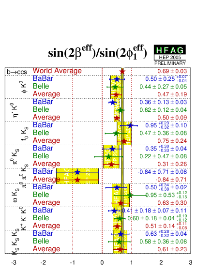
Figure 8: Summary [13] of the BELLE and BABAR results for $\sin\!2\beta_{\rm{eff}}$ obtained from $b\rightarrow s\overline{s}s$-type transitions. The average value obtained for $\sin\!2\beta$ from charmonium modes is also indicated.

6 Overall status

Global fits of the four CKM parameters taking into account the measurements of the three angles $\alpha,\beta$ and $\gamma$, $|V_{ub}|$ and $|V_{cb}|$ CKM matrix elements, ${\rm\Delta}m_{d}$ and ${\rm\Delta}m_{s}$ mixing frequencies and the direct CP violation parameter in the Kaon sector $\epsilon_{K}$) are performed [30], [31]. Besides slightly different theoretical inputs and different statistical treatments both fitters agrees on the $\overline{\rho}$ and $\overline{\eta}$ values :

$$\overline{\rho} \overline{\eta}$$

$$\rm{CKMFitter} 0.208^{+0.038}_{-0.043} 0.337^{+0.024}_{-0.022}$$

$$\rm{UTfit} 0.216\pm 0.036 0.342\pm 0.022$$

An example of a fit output is shown in Figure 9. The fact that all measurements are compatible indicates that the Standard Model provides a coherent picture of the CP violation mechanism and that New Physics should appear as a correction to this framework.

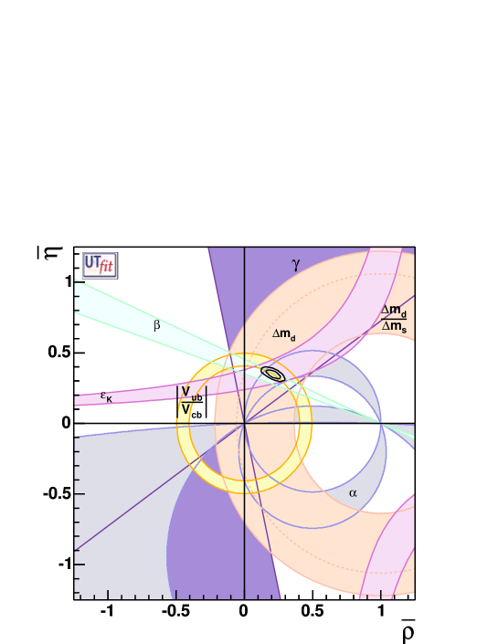
Figure 9: Allowed regions for $\overline{\rho}$ and $\overline{\eta}$ obtained by [31]. The closed contours at 68 % and 95 % probability are shown. The full lines correspond to 95 % probability regions for the individual constraints, given by the measurements of $|V_{ub}|$/$|V_{cb}|$, $\varepsilon_{K}$, ${\rm\Delta}m_{d}$, ${\rm\Delta}m_{s}$, $\alpha,\beta,\gamma$. The dotted curve corresponds to the 95 % upper limit obtained from the experimental study of ${\rm\Delta}m_{s}$.

A simple way to test for the presence of New Physics in the $B_{d}$ mixing in a model independent way is the following :

• Perform a CKM parameters determination using quantities which are involving only tree diagrams, so that they can be considered as “New Physics free”. These quantities are $|V_{ub}|/|V_{cb}|$ and the information on the angle $\gamma$ as obtained from the $B^{-}\rightarrow D^{(*)0}K^{(*)-}$ modes [31].

• parametrise the presence of New Physics by adding two new parameters $r_{d}$ and $\theta_{d}$ : ${\rm\Delta}m_{d}^{\rm{Exp}}=r_{d}^{2}{\rm\Delta}m_{d}^{\rm{SM}}$ and ${\cal A}(J/\Psi K^{0})=\sin(2\beta+2\theta_{d})$, $\alpha^{\rm{Exp}}=\alpha^{\rm{SM}}-\theta_{d}$

• Perform the Unitarity Triangle fit [30], [31] with these extra parameters using all available measurements 

An example of the resulting constraints on $r_{d}$ and $\theta_{d}$ is shown in Figure 10. The large theoretical uncertainty on the non perturbative QCD parameter $f_{B_{d}}\sqrt{\hat{B}_{B_{d}}}$ which is entering in the extraction of the CKM matrix element from the ${\rm\Delta}m_{d}$ measurement explains the fact that despite precise measurements $r_{d}$ is only poorly constrained. The situation is quite different for $\theta_{d}$ : the fit selects $\theta_{d}\sim 0$ which indicates that New Physics CP violating phase should be close to the Standard Model one.

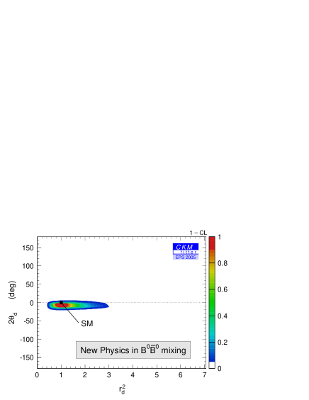
Figure 10: Confidence level obtained on the New Physics parameters $r_{d}$ and $\theta_{d}$. The preferred region is centred on the value corresponding to the Standard Model value ($r_{d}=1$ and $\theta_{d}=0$).

7 Conclusion

Charm and beauty physics are entering the precision era. The non perturbative QCD parameter $f_{D}$ is now precisely measured by CLEO-c and is found to be in good agreement with the latest LQCD computations. The $B\rightarrow\tau\nu$ decay should be measured within the next years, providing a measurement of $f_{B}$. For the first time $b\rightarrow d\gamma$ type decays have been observed, the measurements are not yet precise enough but in the forthcoming years , the ratio of $B\rightarrow\rho\gamma$ to $B\rightarrow K^{*}\gamma$ may provide constraints on $|V_{td}|/|V_{ts}|$ complementary to the mixing measurements. One of the missing measurements is the $B_{s}$ mixing frequency parameter ${\rm\Delta}m_{s}$, if it is not achieved at the Tevatron this will be done at the LHC. The $|V_{ub}|$ measurement using semi-leptonic $B$ decays is now getting quite precise. The inclusive method has reached a precision of 8%, the exclusive one is at the limit of being able to distinguish between theoretical models. CP violation is measured at 5% in the charmonium modes, unfortunately one is not yet able to conclude on the presence or not of New Physics in the $b\rightarrow s\overline{s}s$-type decays, more statistics are needed. The angle $\alpha$ is now measured with a precision of about 10 % using the $B^{0}\rightarrow\rho\rho$ decay. A precision measurement of the angle $\gamma$ will require more data due to the rather small value of the $r_{B}$ parameter. All these measurements tell us that the Standard Model is an excellent description of CP violating and FCNC processes. New Physics in the $B_{d}$ mixing seems to have a CP violation phase close to the Standard Model one. The $B_{s}$ window on new Physics has still to be looked at, this will be one of the most important task of the LHCb experiment at CERN.

8 Acknowledgements

I would like to thank the organisers of this very interesting conference for their invitation in Lisboa. I would also like to thank my BABAR colleagues for their support and help in preparing this talk. Many thanks to the “UT-Fitter” Maurizio Pierini and the “CKM-Fitter” Heiko Lacker for providing me all the results of their programs. I am really indebted to Achille Stocchi for the enlighting discussions we had while preparing this talk and for his continuous support.

References

- [1] N. Cabibbo, Phys. ReV. Lett. 10 (1963) 351.
- [2] M. Kobayashi and T. Maskawa,Prog. Theor. Phys. 49 (1973) 652.
- [3] A.J. Buras, M.E. Lautenbacher and G. Ostermaier, Phys. ReV. D50 (1994) 3433.
- [4] V. V. Anisimovsky, E949 Collaboration, Phys. Rev. Lett. 93, 031801 (2004)
- [5] K. Sakashita, E391a, Kaon 2005 International Workshop, June 2005.
- [6] KTeV, Phys. Rev. Lett. 93, 021805 (2004)
- [7] KTeV, Phys. Rev. Lett. 84, 5279 (2000)
- [8] NA48 Phys. Lett. B 610 (,) 165 (2005).
- [9] KLOE, hep-ex/0505012
- [10] NA48/2, M. Sozzi, Rencontres de Physique de la Vallee d’Aoste 2005, Feb 27-Mar 5 2005
- [11] CLEO-c, CLEO-CONF 05-5
- [12] T.Inami and C.S.Lim, Prog.Theor.Phys. 65 (1981) 297; ibid. 65 (1981) 1772.
- [13] http://www.slac.stanford.edu/xorg/hfag/
- [14] H.G. Moser and A. Roussarie, Nucl. Instum. Meth. A384 (1997) 491.
- [15] CDF-Note 05-03-10, http://www-cdf.fnal.gov/physics/new/bottom/bottom.html
- [16] D0-Note 4881, D0-Note 4878 , http://www-d0.fnal.gov/Run2Physics/WWW/results/b.htm
- [17] N. Leonardo (CDF) and J. Stark (D0), this conference and references therein.
- [18] C. Jessop (BABAR) and D Mohapatra (BELLE), this conference and references therein.
- [19] BABAR Collaboration Phys. Rev. Lett. 94, 011801 (2005)
- [20] BELLE Collaboration hep-ex/0506079
- [21] Proceedings of the CERN workshop on “The CKM matrix and the Unitarity Triangle”, CERN-2003-002-corr and hep-ph/0304132 and references therein.
- [22] A. Limosani (BELLE), G, Della Ricca (BABAR), this conference and references therein.
- [23] BABAR Collaboration hep-ex/0408075
- [24] BELLE Collaboration Phys. Lett. B 621 (,) 28 (2005).
- [25] BABAR Collaboration hep-ex/0506036
- [26] BABAR Collaboration hep-ex/0507017
- [27] BELLE Collaboration hep-ex/0505088
- [28] BELLE Collaboration hep-ex/0508018
- [29] O. Buchmuller and H. Flacher, hep-ph/0507253
- [30] CKMFitter group http://ckmfitter.in2p3.fr, J. Charles et al. Eur. Phys. J. C 41 (,) 1-131,2005.
- [31] UTFit group, http://www.utfit.org, M Bona et al. JHEP 0507 (2005)028, hep-ph/0501199, hep-ph/0509219.
- [32] BABAR Collaboration hep-ex/0507069 hep-ex/0407038
- [33] BELLE Collaboration hep-ex/0507034
- [34] S. Eidelman et al. Phys. Lett. B 592 (,) 1 (2004).
- [35] P. Grenier (BABAR) and O. Tajima (BELLE) this conference and references therein.
- [36] BABAR Collaboration, Phys. Rev. Lett. 94, 161803 (2005)
- [37] BELLE Collaboration hep-ex/0507037
- [38] M. Gronau and D. London, Phys. Lett. B 253 (,) 483 (1991), M. Gronau and D. Wyler, Phys. Lett. B 265 (,) 172 (1991).
- [39] D. Atwood, I. Dunietz and A. Soni, Phys. Rev. Lett. 78, 3257 (1997), M. Gronau Phys. Lett. B 557 (,) 198 (2003).
- [40] A. Giri, Y. Grossman, A. Soffer and J. Zupan, Phys. Rev. D 68, 054018 (2003).
- [41] T. Gershon (BELLE) and V. Tisserand (BABAR), this conference and references therein.
- [42] BABAR Collaboration, hep-ex/0504039 and hep-ex/0507002.
- [43] BELLE Collaboration, Phys. Rev. D 70, 072003 (2004), hep-ex/0411049 and hep-ex/0504013.
- [44] A. Bondar, T. Gershon and P.Krokovny hep-ph/0503174.
- [45] BELLE Collaboration hep-ex/0507065.
- [46] BABAR Collaboration, Phys. Rev. D 71, 032005 (2005), BELLE Collaboration hep-ex/0504030.
- [47] A. Somov (BELLE) and L. M. Mir (BABAR), this conference and references therein.
- [48] C. Yeche (BABAR) and A. Somov (BELLE) this conference and references therein.
- [49] L. M. Mir (BABAR) and J. Dragic (BELLE) this conference and references therein.
- [50] BELLE Collaboration, BELLE-CONF-0528
- [51] BABAR Collaboration, Phys. Rev. Lett. 93, 131801 (2004).
- [52] BABAR Collaboration, hep-ex/0507004
- [53] BELLE Collaboration, hep-ex/0507045
- [54] D. Djumic (BABAR) and K. Trabelsi (BELLE), this conference and references therein.
- [55] M. Beneke, hep-ph/0505075, H. Y. Cheng, C. K. Chua and A. Soni hep-ph/0506268.