Tests of Quantum Chromo Dynamics at $\mathrm{e^{+}e^{-}}$ Colliders

Abstract

The current status of tests of the theory of strong interactions, Quantum Chromo Dynamics (QCD), with data from hadron production in $\mathrm{e^{+}e^{-}}$ annihilation experiments is reviewed. The LEP experiments ALEPH, DELPHI, L3 and OPAL have published many analyses with data recorded on the $\mathrm{Z^{0}}$ resonance at $\sqrt{s}=91.2$ GeV and above up to $\sqrt{s}>200$ GeV. There are also results from SLD at $\sqrt{s}=91.2$ GeV and from reanalysis of data recorded by the JADE experiment at $14\leq\sqrt{s}\leq 44$ GeV. The results of studies of jet and event shape observables, of particle production and of quark gluon jet differences are compared with predictions by perturbative QCD calculations. Determinations of the strong coupling constant $\alpha_{\mathrm{S}}(m_{\mathrm{Z^{0}}})$ from jet and event shape observables, scaling violation and fragmentation functions, inclusive observables from $\mathrm{Z^{0}}$ decays, hadronic $\tau$ decays and hadron production in low energy $\mathrm{e^{+}e^{-}}$ annihilation are discussed. Updates of the measurements are performed where new data or improved calculations have become available. The best value of $\alpha_{\mathrm{S}}(m_{\mathrm{Z^{0}}})$ is obtained from an average of measurements using inclusive observables calculated in NNLO QCD:

$$\alpha_{\mathrm{S}}(m_{\mathrm{Z^{0}}})=0.1211\pm 0.0021$$

where the error is dominated by theoretical systematic uncertainties. The other measurements of $\alpha_{\mathrm{S}}(m_{\mathrm{Z^{0}}})$ are in good agreement with this value. Finally, investigations of the gauge structure of QCD are summarised and the best values for the colour factors are determined:

$$C_{A} = 2.89\pm 0.21$$

$$C_{F} = 1.30\pm 0.09$$

with errors dominated by systematic uncertainties and in good agreement with the expectation from QCD with the SU(3) gauge symmetry.

1 Introduction

The interactions between the constituents of matter are successfully described by the four forces: the weak, electromagnetic and strong forces and the gravitational force. The weak and the strong interactions occur at small atomic to subatomic distances, the electromagnetic interaction is observed at subatomic to macroscopic distances while effects of Gravitation only play a role at macroscopic distances.

The strong interaction, the main focus of this review, is responsible for the existence of all composite elementary particles (hadrons) by providing the binding force between the constituents and also for most of the short lived hadron decays. Furthermore, the binding of protons and neutrons in nuclei may be explained in analogy to chemical binding of molecules based on the strong interaction of the proton and neutron constituents.

The constituents of hadrons are known as partons or quarks. The known spectrum of hadrons can be explained as composites of five (out of a total of six) quark flavours, where each flavour occurs in three variants distinguished by the so-called colour. In table 1 the basic properties of the six known quarks are shown.

Table 1: Basic properties of the six quarks in the standard model

• Generation	1st	2nd	3rd	Charge
  up-type	u (up)	c (charm)	t (top)	+2/3
  down-type	d (down)	s (strange)	b (bottom)	$-$1/3

A dynamic theory of strong interactions at the constituent level, Quantum Chromo Dynamics (QCD), is constructed as a renormalised field theory in close analogy to Quantum Electro Dynamics (QED), the quantum field theory of the electromagnetic interaction, see e.g. [1, 2, 3, 4, 5, 6]. The quarks are viewed as carriers of three different strong charges, referred to as colours. Interactions between colour charged quarks are mediated by gluons, in analogy to the exchange of photons in QED. The theory is constructed to remain invariant under exchange of the three colour charges, i.e. local gauge transformations in the colour space with the SU(3) symmetry. From the requirement of local gauge invariance under SU(3) the special properties of the gluons are derived: there are eight gluons each carrying a colour charge and anti-charge and thus the gluons can directly interact with each other. The gluon-gluon interactions of QCD are not present in QED; QCD is referred to as a non-abelian gauge theory while QED is an example of an abelian gauge theory. For massless quarks the strong coupling constant $\alpha_{\mathrm{S}}$ is the only free parameter of the theory.

Qualitatively, some important properties of QCD already follow from the possibility of direct gluon-gluon interactions. In QED, the scale dependence of the coupling constant $\alpha$, the so-called running, may be seen as a consequence of screening of the bare electric charge due to vacuum polarisation. At small momentum scales, the exchanged photon resolves only a large volume around the bare charge and thus is exposed to stronger charge screening. At large momentum scales a smaller volume is resolved and less charge screening occurs leading to a rising value of the coupling constant. In QCD the effect has the opposite direction, because a cloud of virtual colour charged gluons around a bare colour charge effectively spreads the colour charge over a volume around the quark carrying the bare colour charge. Thus at small momentum scales exchanged gluons interact with an apparently stronger colour charge while at large momentum scales a correspondingly smaller fraction of the colour charge is resolved. In the limit of infinite momentum scales the resolved charge would vanish, leading to the prediction of asymptotic freedom for quarks. At very small momentum scales the resolved colour charge becomes so large that quarks are tightly bound into hadrons; this explains the observation that quarks are confined into hadrons and cannot be observed as free particles in an experiment.

The process of electron positron annihilation into hadrons, $\mathrm{e^{+}e^{-}}\rightarrow\mathrm{hadrons}$, is an ideal laboratory for studies of strong interaction phenomena at the parton, i.e. quark and gluon level, for several reasons:

• There is no interference between the initial and the final state with the consequence that interpretation of the hadronic final state in terms of QCD processes is simplified.

• The four-momentum of the initial state is, in the absence of significant QED initial state radiation (ISR), fully transferred to the final state. In most experiments the electron and positron beams have equal energies such that the centre of mass system (cms) of the final state coincides with the laboratory frame.

• The experimental conditions in $\mathrm{e^{+}e^{-}}$ annihilation are usually rather clean, because in past and existing colliders there were no multiple interactions in a given bunch crossing and backgrounds coming directly from the accelerator like lost beam particles or synchrotron radiation were kept at a low level in the experiments.

• The presently available $\mathrm{e^{+}e^{-}}$ annihilation data allow detailed studies of QCD in a large range of cms energies covering more than an order of magnitude from 12 GeV to 209 GeV. This unique collection of data forms in particular the basis of tests of the energy scale dependence of QCD predictions.

Figure 1 presents an overview of our current understanding of the process $\mathrm{e^{+}e^{-}}\rightarrow\mathrm{hadrons}$. The incoming electron and electron annihilate into an intermediate vector boson, shown as $(\mathrm{Z^{0}}/\gamma)^{*}$, possibly after initial state radiation. The quark pair produced in the vector boson decay will start to radiate gluons which in turn radiate gluons or turn into quark pairs themselves. In this way a so-called parton shower develops until all parton interactions happen at low energy scales of about 1 GeV where confinement and thus hadron formation sets in. The parton shower occupies a volume with radius $\sim 10^{-1}$ fm, according to the uncertainty principle.

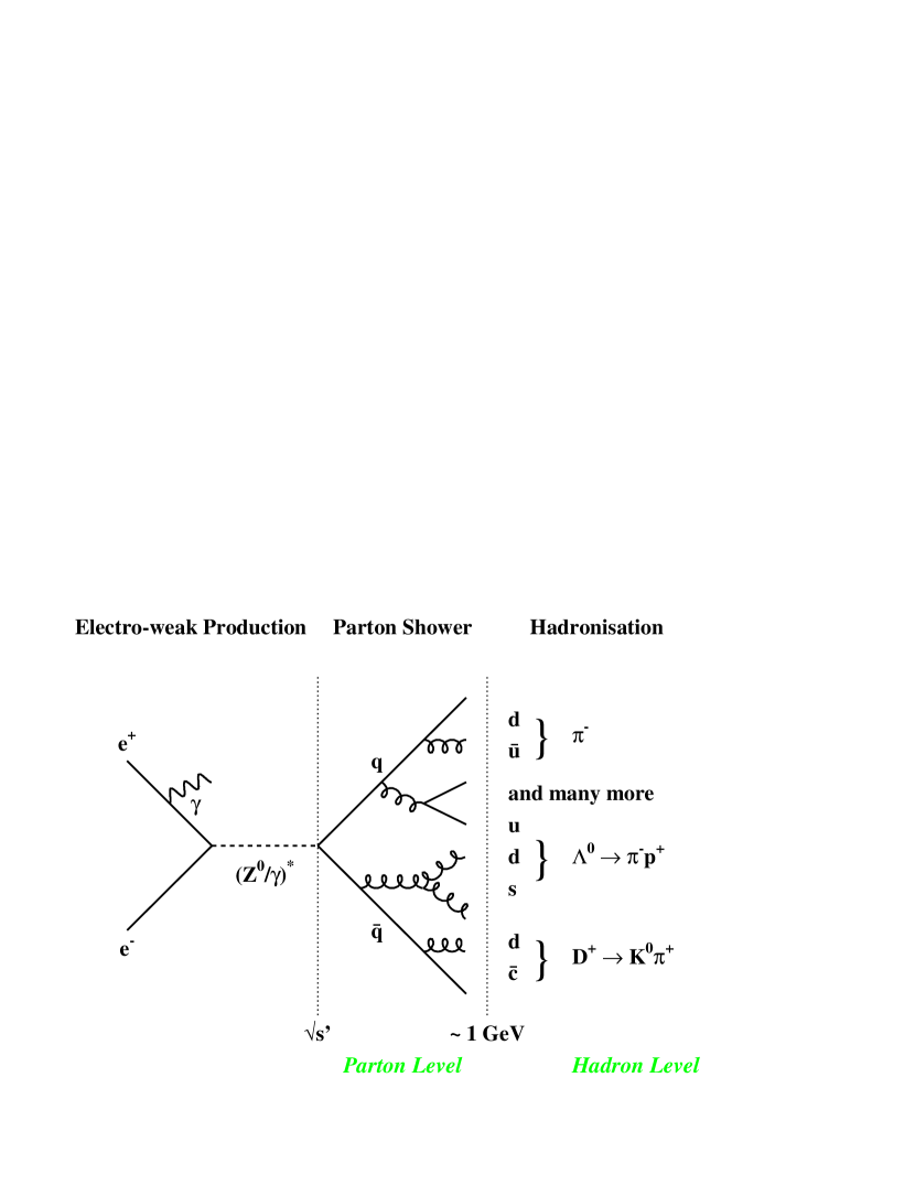
Figure 1: Schematic view of a $\mathrm{e^{+}e^{-}}\rightarrow\mathrm{hadrons}$ event; $\sqrt{s^{\prime}}$ denotes the invariant mass of the hadronic system, usually close the nominal cms energy $\sqrt{s}$ of the experiment.

This review will begin in section 2 with a brief introduction into fundamentals of QCD predictions and section 3 gives a short overview of milestones in the history of QCD tests in $\mathrm{e^{+}e^{-}}$ annihilation together with a summary of the $\mathrm{e^{+}e^{-}}$ colliders and experiments which produced the currently available data. The following section 4 discusses studies based on jet reconstruction algorithms and event shape observables. The subject of section 5 is inclusive particle production and section 6 presents results from inclusive observables. A summary of determinations of the strong coupling $\alpha_{\mathrm{S}}$ is given in section 7 while the properties of jets originating from quarks or gluons are discussed in section 8 Studies of the gauge structure of QCD are reviewed in section 9, followed by conclusions and outlook in section 10.

2 Basics of QCD and hadron production

We collect here the important predictions of QCD which can be studied with data from hadron production in $\mathrm{e^{+}e^{-}}$ annihilation. In QCD with the SU(3) gauge symmetry the following fundamental processes are possible [6, 5]:

Gluon radiation from quarks

This process is the analog of photon bremsstrahlung and occurs with relative strength $C_{F}=4/3$.

Quark pair production

This process is the analog of e.g. $\mathrm{e^{+}e^{-}}$ pair production from a photon and has a relative strength $T_{F}=1/2$. However, it is possible to create quark pairs of all kinematically accessible quark flavours $n_{f}$ and thus the contribution of this process is effectively $T_{F}n_{f}$.

Triple gluon vertex

This process is unique to QCD because the gluons are themselves colour charged, the relative strength is $C_{A}=3$.

There is in addition the quartic gluon vertex which is at least ${\cal O}(\alpha_{\mathrm{S}}^{3})$ in $\mathrm{e^{+}e^{-}}$ annihilation and known to be a negligible contribution to radiative corrections to lower order processes [7]. Figure 2 shows the Feynman diagrams of the three fundamental processes.

Figure 2: Feynman diagrams of the three fundamental QCD processes.

The overall strength of the strong coupling is given by a constant of nature, the strong coupling constant $\alpha_{\mathrm{S}}$. This constant is the only free parameter of the theory when quarks are treated as massless. Therefore many studies of QCD can be formulated as measurements of the strong coupling constant and comparisons of the results for $\alpha_{\mathrm{S}}$ of different analyses give insight into the consistency of the theory.

2.1 Everything runs

2.1.1 Renormalisation scale dependence

The predictions of QCD are finite, because the theory has been renormalised in order to remove divergent terms. The renormalisation introduces a dependence of QCD predictions on the energy scale $\mu$, at which the renormalisation is performed. The renormalisation scale $\mu$ is arbitrary and physical results should be independent of $\mu$. Several prescriptions for renormalisation exist, the so-called renormalisation schemes, and in this report we use the widely adopted $\overline{\mathrm{MS}}$ renormalisation scheme [6, 5] throughout.

A QCD prediction of an observable quantity $R$ measured in $\mathrm{e^{+}e^{-}}$ annihilation, e.g. a differential cross section, can be written as:

$$R=\sum_{n=0}^{\infty}R_{n}\alpha_{\mathrm{S}}^{n}\;\;,$$ (1)

where the $R_{n}$ are the coefficients in $n$th order of the perturbation series. The quantity $R$ depends on $\alpha_{\mathrm{S}}$ and the ratio $x_{\mu}=Q/\mu$ of the physical scale $Q$ of the process and the renormalisation scale $\mu$, for reasons of consistency of the dimension of $R$. In the limit $n\rightarrow\infty$ this dependence on the renormalisation scale is expected to vanish; however, for truncated perturbative calculations a residual dependence will remain. The requirement of renormalisation scale independence is formally expressed as the renormalisation group equation (RGE), also known as Callan-Symanzik equation [8, 9], see e.g. [5]:

$$\mu^{2}\frac{\mathrm{d}}{\mathrm{d}\mu^{2}}R\left(x_{\mu}^{2},\alpha_{\mathrm{S}}\right)=\mu^{2}\left(\frac{\partial}{\partial\mu^{2}}+\frac{\partial\alpha_{\mathrm{S}}}{\partial\mu^{2}}\frac{\partial}{\partial\alpha_{\mathrm{S}}}\right)R=0\;\;.$$ (2)

The renormalisation scale dependence of the coefficients $R_{n}$ will be compensated by a renormalisation scale dependence of the coupling constant $\alpha_{\mathrm{S}}(\mu)$:

$$\mu^{2}\frac{\partial\alpha_{\mathrm{S}}}{\partial\mu^{2}}=\beta(\alpha_{\mathrm{S}}(\mu^{2}))=-\beta_{0}\alpha_{\mathrm{S}}^{2}(\mu^{2})-\beta_{1}\alpha_{\mathrm{S}}^{3}(\mu^{2})-\beta_{2}\alpha_{\mathrm{S}}^{4}(\mu^{2})+\mbox{${\cal O}(\alpha_{\mathrm{S}}^{5})$}\;\;.$$ (3)

Equation (3) introduces the $\beta$-function of QCD, with coefficients [5]

$$\beta_{0} = \frac{11C_{A}-4T_{F}n_{f}}{12\pi}\;\;,$$ (4)

$$\beta_{1} = \frac{17C_{A}^{2}-5C_{A}n_{f}-3C_{F}n_{f}}{24\pi^{2}}\;\;\mathrm{and}$$

$$\beta_{2} = \frac{2857C_{A}^{3}+(54C_{F}^{2}-615C_{F}C_{A}-1415C_{A}^{2})n_{f}+(66C_{F}+79C_{A})n_{f}^{2}}{3456\pi^{3}}\;\;.$$

The coefficient $\beta_{2}$ depends on the renormalisation scheme and is shown here for the $\overline{\mathrm{MS}}$ scheme. The variable $n_{f}$ specifies the number of active quark flavours which are considered in the calculation and thus from kinematics it depends on the energy scale of the process. At low energies below the thresholds for heavy quark production direct contributions as well as contributions to radiative corrections are suppressed resulting in $n_{f}=3$. When with increasing energy scale a heavy quark production threshold is crossed $n_{f}$ must be increased by one unit, see section 2.1.4 below.

Combining equations (1), (2) and (3) results in

$$0 = \mu^{2}\frac{\partial R_{0}}{\partial\mu^{2}}+\alpha_{\mathrm{S}}(\mu^{2})\mu^{2}\frac{\partial R_{1}}{\partial\mu^{2}}+\alpha_{\mathrm{S}}^{2}(\mu^{2})\left(\mu^{2}\frac{\partial R_{2}}{\partial\mu^{2}}-R_{1}\beta_{0}\right)+$$

$$\alpha_{\mathrm{S}}^{3}(\mu^{2})\left(\mu^{2}\frac{\partial R_{3}}{\partial\mu^{2}}-(R_{1}\beta_{1}+2R_{2}\beta_{0})\right)+\ldots\;\;.$$

A solution for equation (2.1.1) can be found by demanding that the coefficients of $\alpha_{\mathrm{S}}^{n}$ vanish for all orders $n$. After integration from a specific choice of renormalisation scale $\mu_{\mathrm{R}}^{2}$ to another scale $Q^{2}$ the coefficients can be written as

$$R_{0} = const.\;\;,$$ (6)

$$R_{1} = const.\;\;,$$

$$R_{2}(x_{\mu}^{2}) = R_{2}(1)+\beta_{0}R_{1}\ln x_{\mu}^{2}\;\;\mathrm{and}$$

$$R_{3}(x_{\mu}^{2}) = R_{3}(1)+(2R_{2}(1)\beta_{0}+R_{1}\beta_{1})\ln x_{\mu}^{2}+R_{1}\beta_{0}^{2}\ln^{2}x_{\mu}^{2}$$

with $x_{\mu}=Q/\mu_{\mathrm{R}}$. The $R_{i}(1)$ are the coefficients evaluated at the renormalisation scale $\mu_{\mathrm{R}}$. We note that all coefficients $R_{n},n\geq 2$ depend explicitly on the renormalisation scale parameter $x_{\mu}$. However, the coefficients $R_{n}(x_{\mu})$ only depend on $x_{\mu}$ via terms containing $\ln x_{\mu}^{2}$. This observation has the important consequence that QCD predictions for physical observables at any scale given by $x_{\mu}$ can be computed in terms of constant coefficients derived using the renormalisation scale given at $x_{\mu}=1$. The scale dependence of the prediction then enters only through the scale dependent strong coupling constant $\alpha_{\mathrm{S}}(Q^{2})$.

The choice of the renormalisation scheme (RS) is arbitrary and usually dictated by convenience to perform a calculation. It is also evident that a result of a QCD prediction for a physical observable like a cross section should in principle not depend on the choice of RS. In practice with perturbative predictions truncated at e.g. 2nd or 3rd order there are significant dependences on the RS which may be interpreted as indications of the size of missing higher order terms.

This problem and attempts to provide solutions have already been discussed more than 20 years ago when the first next-to-leading (NLO) QCD calculations became available [10, 11, 12, 13, 14]. Three different ways to choose an “optimal” renormalisation scheme or scale for sufficiently inclusive observables depending on a single energy scale were devised, see e.g. [15] for a review. Examples for such observables are mean values (or higher moments) of event shape distributions or $R_{\mathrm{e^{+}e^{-}}}$. It is important to note that at NLO a variation of the renormalisation scale is equivalent to a variation of the RS yielding the same results [16]. The three methods for choosing an optimal renormalisation scheme are the following:

Principle of minimum sensitivity (PMS)

The principle of minimum sensitivity is based on the observation that at a given order all possible RSs can be labelled by their renormalisation point (scale) $x_{\mu}$ and the coefficients of their $\beta$-functions [12]. Now one may find the RS for which a QCD prediction $R(\alpha_{\mathrm{S}})$ for a physical observable has minimal sensitivity w.r.t. choosing a RS. This corresponds to a stationary point of the function $R(\alpha_{\mathrm{S}},l_{i})$ with the RS labels $l_{i}$. At NLO finding a stationary point of $R(\alpha_{\mathrm{S}},x_{\mu})$ is sufficient, since at this order the coefficients of the $\beta$-function are universal.

Method of effective charges (ECH)

Using the freedom to choose the RS the perturbative expansion is rearranged such that higher order terms vanish. The running coupling absorbs all scale dependent effects and becomes a process dependent so-called effective charge which satisfies a generalised $\beta$-function [10, 11]. This method is also referred to as “fastest apparent convergence” or FAC. At NLO a convenient way to find the FAC scheme is to find the value of $x_{\mu}$ for which the complete $\mathcal{O}(\alpha_{\mathrm{S}}^{2})$ term vanishes.

Brodsky-Lepage-Mackenzie method (BLM)

The BLM method proposes to adjust the renormalisation point (scale) $x_{\mu}$ for a given RS such that the dependence of the NLO term on the number of quark flavours $n_{f}$ is cancelled [13, 17]. This prescription implies that vacuum polarisation corrections due to fermion pairs are absorbed by the running coupling $\alpha_{\mathrm{S}}(\mu)$.

2.1.2 The running strong coupling constant

The scale dependence or running of the strong coupling constant can be derived by integrating equation (3) to obtain an expression relating values of $\alpha_{\mathrm{S}}$ at two different scales $Q$ and $\mu_{\mathrm{R}}$. Since the choice of renormalisation scale is arbitrary the expressions can be used to relate values of $\alpha_{\mathrm{S}}$ at any two scales. Solutions differ according to how many orders (often referred to as the number of loops) in perturbation theory have been considered in the calculation of the $\beta$-function. The first term corresponds to one order (loop), the second to two orders (loops), etc. The solutions valid for one and two loops are:

$$\alpha_{\mathrm{S}}(Q^{2})=\frac{\alpha_{\mathrm{S}}(\mu_{\mathrm{R}}^{2})}{1+\alpha_{\mathrm{S}}(\mu_{\mathrm{R}}^{2})\beta_{0}\ln x_{\mu}^{2}}\;\;\mathrm{and}$$ (7)

$$\beta_{0}\ln x_{\mu}^{2}=\frac{1}{\alpha_{\mathrm{S}}(Q^{2})}-\frac{1}{\alpha_{\mathrm{S}}(\mu_{\mathrm{R}}^{2})}+\frac{\beta_{1}}{\beta_{0}}\ln\left(\frac{\alpha_{\mathrm{S}}(Q^{2})}{\alpha_{\mathrm{S}}(\mu_{\mathrm{R}}^{2})}\cdot\frac{\beta_{0}+\beta_{1}\alpha_{\mathrm{S}}(\mu_{\mathrm{R}}^{2})}{\beta_{0}+\beta_{1}\alpha_{\mathrm{S}}(Q^{2})}\right)\;\;.$$ (8)

The 2-loop solution shown in equation (8) may be solved numerically for $\alpha_{\mathrm{S}}(Q^{2})$. The solution for a 3-loop $\beta$-function is also found directly by integrating equation (3):

$$\beta_{0}\ln x_{\mu}^{2}=F(\alpha_{\mathrm{S}}(Q))-F(\alpha_{\mathrm{S}}(\mu_{\mathrm{R}}))\;\;.$$ (9)

The function $F(\alpha_{\mathrm{S}})=\beta_{0}\int-1/(\beta_{0}\alpha_{\mathrm{S}}^{2}+\beta_{1}\alpha_{\mathrm{S}}^{3}+\beta_{2}\alpha_{\mathrm{S}}^{4})\,\mathrm{d}\alpha_{\mathrm{S}}$ is for $n_{f}\leq 5$, i.e. $\beta_{2}>0$, given by

$$F(\alpha_{\mathrm{S}}) = \frac{1}{\alpha_{\mathrm{S}}}-\frac{\beta_{1}^{2}-2\beta_{0}\beta_{2}}{\beta_{0}\sqrt{-\beta_{1}^{2}+4\beta_{0}\beta_{2}}}\arctan\left(\frac{\beta_{1}+2\beta_{2}\alpha_{\mathrm{S}}}{\sqrt{-\beta_{1}^{2}+4\beta_{0}\beta_{2}}}\right)$$

$$+\frac{\beta_{1}\log(\alpha_{\mathrm{S}})}{\beta_{0}}-\frac{\beta_{1}\log(\beta_{0}+\beta_{1}\alpha_{\mathrm{S}}+\beta_{2}\alpha_{\mathrm{S}}^{2})}{2\beta_{0}}\;\;.$$

As before equation (9) may be solved numerically for $\alpha_{\mathrm{S}}(Q)$. For the case $n_{f}\geq 6$ we have $\beta_{2}<0$ and the second term of the RHS of equation (2.1.2) is rewritten to contain only real terms with $z=(\beta_{1}+2\beta_{2}\alpha_{\mathrm{S}})/\sqrt{\beta_{1}^{2}-4\beta_{0}\beta_{2}}$:

$$-\frac{\beta_{1}^{2}-2\beta_{0}\beta_{2}}{\beta_{0}\sqrt{\beta_{1}^{2}-4\beta_{0}\beta_{2}}}\frac{1}{2}\log\frac{1+z}{1-z}\;\;.$$ (11)

The case $n_{f}=6$ becomes relevant when an evolution of $\alpha_{\mathrm{S}}$ to energy scales above the threshold for t quark production is performed.

The perturbative running of the strong coupling constant breaks down at sufficiently small scales $Q$ such that e.g. in LO $\alpha_{\mathrm{S}}(\mu_{\mathrm{R}}^{2})\beta_{0}\ln x_{\mu}^{2}=-1$. At such low scales values of the strong coupling are $\alpha_{\mathrm{S}}>1$ and thus perturbative expansions in $\alpha_{\mathrm{S}}$ will fail to converge. The value of $Q=\Lambda_{\mathrm{QCD}}$ where this breakdown of perturbative QCD occurs is known as the Landau pole. Since typical light hadron masses are ${\cal O}(100)$ MeV one might expect that $\Lambda_{\mathrm{QCD}}$ has similar values. Using the LO equation (7) this yields $\alpha_{\mathrm{S}}(m_{\mathrm{Z^{0}}})\approx 0.1$ and $\alpha_{\mathrm{S}}(1~{}\mathrm{GeV}^{2})\approx 0.2$ which sets a rough lower limit for the applicability of perturbative QCD.

2.1.3 Running quark masses

QCD predictions discussed so far are valid for massless quarks. However, it is well known that quarks have masses ranging from ${\cal O}(1)$ MeV for the light u and d quarks to about 174 GeV for the t quark [18]. Mass effects are incorporated into the theory via mass terms in the Lagrangian which are subject to renormalisation like the coupling constant. The requirement of independence of QCD predictions from the renormalisation scale introduces in the presence of a quark mass a new term into the RGE equation (2):

$$\mu^{2}\left(\frac{\partial}{\partial\mu^{2}}+\frac{\partial\alpha_{\mathrm{S}}}{\partial\mu^{2}}\frac{\partial}{\partial\alpha_{\mathrm{S}}}+\frac{\partial m}{\partial\mu^{2}}\frac{\partial}{\partial m}\right)R=0$$ (12)

with

$$\mu^{2}\frac{\partial m}{\partial\mu^{2}}=-\gamma_{m}(\mu^{2})m(\mu^{2})$$ (13)

where $\gamma_{m}(\mu^{2})$ is the so-called mass anomalous dimension. The mass anomalous dimension $\gamma_{m}$ has been calculated as a power series in the strong coupling constant, $\gamma_{m}(\alpha_{\mathrm{S}})=\gamma_{0}\alpha_{\mathrm{S}}+\gamma_{1}\alpha_{\mathrm{S}}^{2}+\mbox{${\cal O}(\alpha_{\mathrm{S}}^{3})$}$, with coefficients $\gamma_{0}=1/\pi$ and $\gamma_{1}=(303-10n_{f})/(72\pi^{2})$ in the $\overline{\mathrm{MS}}$ renormalisation scheme [19].

Integrating equation (13) and substituting $\alpha_{\mathrm{S}}(\mu_{\mathrm{R}}^{2})$ for $\mu_{\mathrm{R}}^{2}$ gives an equation for the running quark mass:

$$m(Q^{2})=m(\mu_{\mathrm{R}}^{2})\exp\left(\int_{\alpha_{\mathrm{S}}(\mu_{\mathrm{R}}^{2})}^{\alpha_{\mathrm{S}}(Q^{2})}\frac{\gamma_{m}(\alpha_{\mathrm{S}})}{\beta(\alpha_{\mathrm{S}})}\mathrm{d}\alpha_{\mathrm{S}}\right)\;\;.$$ (14)

Solutions to equation (14) in the $\overline{\mathrm{MS}}$ renormalisation scheme are e.g. given in [19].

2.1.4 Heavy quark thresholds

The evolution of the strong coupling constant, equation (3), and the quark masses, equation (14), depends on the number of active quark flavours $n_{f}$ through the coefficients of the QCD $\beta$-function and mass anomalous dimension, respectively. When an evolution of e.g. $\alpha_{\mathrm{S}}(\mu^{2})$ across the excitation threshold $\mu_{\mathrm{q}}$ for production of heavy quark pairs is attempted an explicit treatment of the changing number of flavours, $n_{f}\rightarrow n_{f}+1$, is necessary.

One requires that the theory at scales below the heavy quark threshold $\mu_{\mathrm{q}}$ with $n_{f}$ active quark flavours is consistent with the theory at scales above $\mu_{\mathrm{q}}$ with $n_{f}+1$ active quark flavours [20]. This results in matching conditions for the strong coupling constant at the heavy quark threshold; these are $\alpha_{\mathrm{S}}(n_{f})=\alpha_{\mathrm{S}}(n_{f}+1)$ in LO (leading order) and NLO. At the next order the matching involves a discontinuity of the value of the strong coupling constant at the heavy quark threshold $\mu_{\mathrm{q}}$:

$$\alpha_{\mathrm{S}}(n_{f},\mu_{\mathrm{q}})=\alpha_{\mathrm{S}}(n_{f}+1,\mu_{\mathrm{q}})+\alpha_{\mathrm{S}}^{3}(n_{f}+1,\mu_{\mathrm{q}})c_{2}\;\;,$$ (15)

where the value of the coefficient $c_{2}$ depends on the definition of the heavy quark mass. For the running $\overline{\mathrm{MS}}$ mass, i.e. $\mu_{\mathrm{q}}=m_{\mathrm{q},\overline{\mathrm{MS}}}(m_{\mathrm{q},\overline{\mathrm{MS}}})$, one has $c_{2}=11/(72\pi^{2})$ while for the pole mass $M_{\mathrm{q}}$ with $\mu_{\mathrm{q}}=M_{\mathrm{q}}$ one has $c_{2}=-7/(24\pi^{2})$ [20].

In this report we use 3-loop running of the strong coupling constant as explained in section 2.1.2 together with matching at heavy quark thresholds using equation (15) and $\overline{\mathrm{MS}}$ masses $m_{c,\overline{\mathrm{MS}}}(m_{c,\overline{\mathrm{MS}}})=1.25$ GeV and $m_{b,\overline{\mathrm{MS}}}(m_{b,\overline{\mathrm{MS}}})=4.25$ GeV [18] when a value of $\alpha_{\mathrm{S}}$ is evolved from an energy scale $Q_{1}$ to another scale $Q_{2}$.

2.2 Perturbative QCD

Predictions of perturbative QCD are possible for observables which fulfil the Sterman-Weinberg criteria of infrared and collinear safety [21]: an observable is infrared and collinear safe when its value is not affected by the emission of low-momentum partons or by the replacement of a parton by collinear partons with the same total 4-momentum. For such observables predictions as power series in the strong coupling $\alpha_{\mathrm{S}}$ may be performed.

The observables typically used in studies of $\mathrm{e^{+}e^{-}}$ annihilation to hadrons may be classified as follows:

exclusive

Exclusive observables derived from jet clustering algorithms or based on event shape definitions (see section 4 for details) classify the hadronic final states according to their topology. Measurements of differential cross sections for such observables may be compared with corresponding QCD predictions.

semi-inclusive

With semi-inclusive observables all hadronic final states are considered and average properties of the produced hadrons such as particle multiplicity or momentum spectra are studied.

inclusive

The inclusive observables are simply based on counting of hadronic final states. Examples are the hadronic widths of the $\mathrm{Z^{0}}$ boson or the $\tau$ lepton or the total cross section for hadron production in $\mathrm{e^{+}e^{-}}$ annihilation.

Most exclusive observables used in hadron production from $\mathrm{e^{+}e^{-}}$ annihilation are sensitive to the non-collinear emission of a single energetic (or hard) gluon. The corresponding final state is expected to consist of three separated bundles of particles referred to as jets and originating from the quarks and gluon produced in the $\mathrm{e^{+}e^{-}}$ interaction. These observables will be referred to as 3-jet observables. Some observables are defined such that they are only sensitive to 4-jet final states, i.e. those involving one gluon emission and one of the fundamental QCD processes listed above, and will be referred to 4-jet observables.

2.2.1 Fixed order predictions

The basic prediction in NLO for the normalised differential distribution of a 3-jet observable $y$ is given by a power series in $\hat{\alpha}_{\mathrm{S}}(Q)=\alpha_{\mathrm{S}}(Q)/(2\pi)$:

$$\frac{1}{\sigma_{\mathrm{tot}}}\frac{\mathrm{d}\sigma}{\mathrm{d}y}=\frac{\mathrm{d}A}{\mathrm{d}y}\hat{\alpha}_{\mathrm{S}}(Q)+\left(\left(2\pi\beta_{0}\ln(x_{\mu}^{2})-2\right)\frac{\mathrm{d}A}{\mathrm{d}y}+\frac{\mathrm{d}B}{\mathrm{d}y}\right)\hat{\alpha}_{\mathrm{S}}^{2}(Q)\;\;.$$ (16)

The energy scale $Q$ at which the strong coupling is evaluated is generally identified with the physical hard scale of the process such as the cms energy of the $\mathrm{e^{+}e^{-}}$ annihilation. The coefficient functions $\mathrm{d}A/\mathrm{d}y$ and $\mathrm{d}B/\mathrm{d}y$ correspond to the coefficients $R_{1}$ and $R_{2}$ of equation (1) and their renormalisation scale dependence is given by equation (6) after replacing $\alpha_{\mathrm{S}}$ by $\hat{\alpha}_{\mathrm{S}}$ and absorbing $(2\pi)^{n}$ in the coefficient $R_{n}$. The normalisation to the total hadronic cross section $\sigma_{\mathrm{tot}}$ has been accounted for by the relation $\sigma_{\mathrm{tot}}=\sigma_{\mathrm{0}}(1+2\hat{\alpha}_{\mathrm{S}})$ [22]. The coefficient functions $\mathrm{d}A/\mathrm{d}y$ and $\mathrm{d}B/\mathrm{d}y$ may be derived numerically for any suitable observable [23, 24]. The derivation is done by Monte Carlo integration of the NLO QCD matrix elements for the production of up to four partons [22] over contours in phase space given by the definition of the observable $y$. In some cases the LO terms $\mathrm{d}A/\mathrm{d}y$ have been obtained analytically, see e.g. [5].

A third order term $\sim\mathrm{d}C/\mathrm{d}y\hat{\alpha}_{\mathrm{S}}^{3}$ can be added to equation (16) once a numerical integration of the corresponding next-to-next-to-leading order (NNLO) QCD matrix elements is available to generate the NNLO coefficient function $\mathrm{d}C/\mathrm{d}y$ [25, 26]. The renormalisation scale dependence will be expressed as in equation (6) while the normalisation to the total hadronic cross section must now consider $\sigma_{\mathrm{tot}}=\sigma_{\mathrm{0}}(1+2\hat{\alpha}_{\mathrm{S}}+5.6368\hat{\alpha}_{\mathrm{S}}^{2})$ [27]. The complete result for the NNLO term is

$$\left(\frac{\mathrm{d}C}{\mathrm{d}y}+\left(4\pi\beta_{0}\frac{\mathrm{d}B}{\mathrm{d}y}+(2\pi)^{2}\beta_{1}\frac{\mathrm{d}A}{\mathrm{d}y}\right)\ln x_{\mu}^{2}+\left(2\pi\beta_{0}\ln x_{\mu}^{2}\right)^{2}\frac{\mathrm{d}A}{\mathrm{d}y}\right.$$ (17)

$$\left.-2\left(\frac{\mathrm{d}B}{\mathrm{d}y}+2\pi\beta_{0}\ln x_{\mu}^{2}\frac{\mathrm{d}A}{\mathrm{d}y}\right)-1.6368\frac{\mathrm{d}A}{\mathrm{d}y}\right)\hat{\alpha}_{\mathrm{S}}^{3}(Q)\;\;.$$

For 4-jet observables NLO fixed order predictions are also available [28, 29]. Their form is derived from equations (16) and (17) by setting $\mathrm{d}A/\mathrm{d}y=0$:

$$\frac{1}{\sigma_{\mathrm{tot}}}\frac{\mathrm{d}\sigma}{\mathrm{d}y}=\frac{\mathrm{d}B}{\mathrm{d}y}\hat{\alpha}_{\mathrm{S}}^{2}(Q)+\left(\left(4\pi\beta_{0}\ln(x_{\mu}^{2})-2\right)\frac{\mathrm{d}B}{\mathrm{d}y}+\frac{\mathrm{d}C}{\mathrm{d}y}\right)\hat{\alpha}_{\mathrm{S}}^{3}(Q)\;\;.$$ (18)

2.2.2 NLLA predictions

The NLO predictions described above work well in regions of phase space where radiation of a single hard gluon dominates. For configurations with soft or collinear gluon radiation from the initial quark-antiquark pair the Sterman-Weinberg criteria may not be fulfilled anymore and consequently new divergent terms appear. For observables $y$ defined to vanish when no gluon radiation occurred, i.e. in the 2-jet limit, the typical leading behaviour of the cumulative cross section $R(y)=\int_{0}^{y}1/\sigma\mathrm{d}\sigma/\mathrm{d}y^{\prime}\,\mathrm{d}y^{\prime}$ is:

$$R(y)\sim\alpha_{\mathrm{S}}^{n}\ln^{2n}\frac{1}{y}=\alpha_{\mathrm{S}}^{n}L^{2n}\;\;,$$ (19)

for each order $n$ of the expansion in $\alpha_{\mathrm{S}}$ with $\ln(1/y)=L$ [30]. For $y\rightarrow 0$ the simple NLO prediction will be unreliable as $\alpha_{\mathrm{S}}L^{2}\ll 1$ will not hold anymore. A systematic analytic resummation of the leading logarithmic terms $\sim L^{2n}$ and the next-to-leading logarithmic terms $\sim L^{2n-1}$ to all orders in $\alpha_{\mathrm{S}}$ has been performed for a special class of observables [30]. Such observables exponentiate, which means that $\ln R(y)\approx Lg_{1}(\alpha_{\mathrm{S}}L)$ and $g_{1}$ has a power series expansion in $\alpha_{\mathrm{S}}L$ [30]. For the cumulative cross section the following representation is possible:

$$R(y) = C(\alpha_{\mathrm{S}})\Sigma(y,\alpha_{\mathrm{S}})+D(y,\alpha_{\mathrm{S}})$$ (20)

$$C(\alpha_{\mathrm{S}}) = 1+\sum_{n=1}^{\infty}C_{n}\hat{\alpha}_{\mathrm{S}}^{n}$$

$$\ln\Sigma(y,\alpha_{\mathrm{S}}) = \sum_{n=1}^{\infty}\sum_{m=1}^{n+1}G_{nm}\hat{\alpha}_{\mathrm{S}}^{n}L^{m}$$

$$= Lg_{1}(\alpha_{\mathrm{S}}L)+g_{2}(\alpha_{\mathrm{S}}L)+\ldots$$

where $\lim_{y\rightarrow 0}D(y,\alpha_{\mathrm{S}})=0$. The function $g_{1}$ contains the resummation of all leading terms $\sim\alpha_{\mathrm{S}}^{n}L^{n+1}$ (LL) while $g_{2}$ resums all next-to-leading terms $\sim\alpha_{\mathrm{S}}^{n}L^{n}$ (NLL). The description of equation (20) is expected to be valid in the region $\alpha_{\mathrm{S}}L<1$ which goes further into the 2-jet region at small values of $y$ than the NLO prediction bounded by $\alpha_{\mathrm{S}}L^{2}\ll 1$.

A general numerical method for performing the resummation for a large class of event shape observables has been presented in [31]. This makes resummation possible in cases where a purely analytical calculation is impossible or too difficult.

2.2.3 Matched NLLA and fixed order predictions

The NLO and NLLA predictions described above can be combined to yield a prediction which is valid in the 2- and 3-jet regions. In order to avoid double counting of terms $\sim\alpha_{\mathrm{S}}$ and $\sim\alpha_{\mathrm{S}}^{2}$ present in both NLO and NLLA predictions one has to identify and remove such terms from the NLLA prediction. Table 2 presents a comparison of the fixed order with the NLLA prediction for the quantity $\ln R(y)$.

Table 2: Comparison of NLLA and fixed order calculations. The dependence of the coefficient functions A, B, and C on $y$ has been suppressed.

• LL	NLL	subleading	non-log	fixed order
  $G_{12}\hat{\alpha}_{\mathrm{S}}L^{2}$	$G_{11}\hat{\alpha}_{\mathrm{S}}L$		$\sim\alpha_{\mathrm{S}}$	$=A\hat{\alpha}_{\mathrm{S}}$
  $G_{23}\hat{\alpha}_{\mathrm{S}}^{2}L^{3}$	$G_{22}\hat{\alpha}_{\mathrm{S}}^{2}L^{2}$	$G_{21}\hat{\alpha}_{\mathrm{S}}^{2}L$	$\sim\alpha_{\mathrm{S}}^{2}$	$=(B-\frac{1}{2}A^{2})\hat{\alpha}_{\mathrm{S}}^{2}$
  $G_{34}\hat{\alpha}_{\mathrm{S}}^{3}L^{4}$	$G_{33}\hat{\alpha}_{\mathrm{S}}^{3}L^{3}$	$G_{32}\hat{\alpha}_{\mathrm{S}}^{3}L^{2}+G_{31}\hat{\alpha}_{\mathrm{S}}^{3}L$	$\sim\alpha_{\mathrm{S}}^{3}$	$=(C-AB+\frac{1}{3}A^{3})\hat{\alpha}_{\mathrm{S}}^{3}$
  ⋮	⋮	⋮	⋮	⋮
  $Lg_{1}(\alpha_{\mathrm{S}}L)$	$g_{2}(\alpha_{\mathrm{S}}L)$	$+\ldots$	$+\ldots$	$=\ln R(y)$

The first two columns represent the resummation of leading and next-to-leading logarithmic terms while the equalities in the last column refer to summing each corresponding row. The coefficient functions $A(y)$, $B(y)$ and $C(y)$ correspond to the cumulative cross sections, e.g. $A(y)=\int_{0}^{y}\mathrm{d}A/\mathrm{d}y^{\prime}\mathrm{d}y^{\prime}$ and analogously for $B(y)$ and $C(y)$. The normalisation of the coefficient functions is such that $A(y_{\mathrm{max}})=B(y_{\mathrm{max}})=C(y_{\mathrm{max}})=0$ where $y_{\mathrm{max}}$ is the maximum kinematically possible value of the observable. This normalisation generates all terms needed to account for the normalisation of the prediction to the total hadronic cross section $\sigma_{\mathrm{tot}}$. The $G_{nm}$ coefficients in the first two rows are determined by expanding the functions $g_{1}$ and $g_{2}$ in terms of $\alpha_{\mathrm{S}}$ while subleading logarithmic terms can be determined numerically [30, 32, 33].

The resulting matched prediction is for the cumulative cross section:

$$\ln R(y) = A(y)\hat{\alpha}_{\mathrm{S}}+(B(y)-\frac{1}{2}A^{2}(y))\hat{\alpha}_{\mathrm{S}}^{2}$$

$$+Lg_{1}(\alpha_{\mathrm{S}}L)+g_{2}(\alpha_{\mathrm{S}}L)$$

$$-(G_{12}L^{2}+G_{11}L)\hat{\alpha}_{\mathrm{S}}-(G_{32}L^{2}+G_{22}L)\hat{\alpha}_{\mathrm{S}}^{2}\;\;.$$

Renormalisation scale dependence and normalisation to the total hadronic cross section can be inserted into equation (2.2.3) by making the replacements $B(y)\rightarrow B(y)+2A(y)(\pi\beta_{0}\ln x_{\mu}^{2}-1)$ and $G_{22}\rightarrow G_{22}+G_{12}2\pi\beta_{0}\ln x_{\mu}^{2}$ as well as modifying $g_{2}$ according to [30], equation (8). This form of matching is referred to as $\ln(R)$-matching. Other forms of matching are possible with small differences in the treatment of higher order terms [30, 34, 35]. An important difference between the $\ln(R)$-matching and other matching schemes is that in the other schemes the coefficients $C_{1}$ and $C_{2}$ and in some cases $G_{21}$ must be known explicitly.

In order to force the NLLA terms to vanish at the upper kinematic limit $y_{\mathrm{max}}$ of an observable $y$ the so-called modified matching is used [30, 35]. The modified matching consists of replacing $L=\ln(1/y)$ by $L^{\prime}=\ln(1+1/y-1/y_{\mathrm{max}})$.

A possible NNLO term in the fixed order prediction as discussed above can be taken into account in the $\ln(R)$-matching scheme by adding the following term to the right-hand-side (RHS) of equation (2.2.3):

$$\left(C(y)-A(y)B(y)+\frac{1}{3}A^{3}(y)-G_{34}L^{4}-G_{33}L^{3}\right)\hat{\alpha}_{\mathrm{S}}^{3}\;\;.$$ (22)

Renormalisation scale dependence and normalisation to the total hadronic cross section can be considered by replacing $C(y)=\int_{0}^{y}\mathrm{d}C/\mathrm{d}y^{\prime}\mathrm{d}y^{\prime}$ by the correspondingly integrated equation (17) and by the replacement $G_{33}\rightarrow G_{33}+G_{23}4\pi\beta_{0}\ln x_{\mu}^{2}$. For matching schemes other than the $\ln(R)$-matching the coefficients $C_{i},i=1,2,3$, $G_{21}$ and in some cases $G_{3i},i=2,1$ must be available.

2.3 Inclusive observables

In the definition of inclusive observables no requirements on the structure of the hadronic events are made, instead the cross sections or branching ratios for the production of hadronic final states are considered. The objects of interest are QCD induced corrections to electro-weak processes with hadronic final states.

The total hadronic cross section in $\mathrm{e^{+}e^{-}}$ annihilation $\sigma_{\mathrm{0}}$ including $\gamma-\mathrm{Z^{0}}$ interference but without QCD corrections can be written as follows (see e.g. [5]):

$$\sigma_{\mathrm{0}}(s)=\frac{4\pi\alpha^{2}}{3s}\left[Q_{f}^{2}-2Q_{f}V_{e}V_{f}\chi_{1}(s)+(A_{e}^{2}+V_{e}^{2})(A_{f}^{2}+V_{f}^{2})\chi_{2}(s)\right]\;\;,$$ (23)

where $\alpha$ is the QED coupling, $Q_{f}$ is the fermion charge and the $A_{f}$ and $V_{f}$ are the axial and vector couplings of fermions to the $\mathrm{Z^{0}}$. These are given by $A_{f}=T_{f,3}$ and $V_{f}=T_{f,3}-2Q_{f}\sin^{2}\Theta_{W}$ with $T_{f,3}=+1/2$ for neutral leptons and up-type quarks and $T_{f,3}=-1/2$ for charged leptons and down-type quarks with the electro-weak mixing angle $\Theta_{W}$. The functions $\chi_{1}=\kappa s(s-m_{\mathrm{Z^{0}}}^{2})/((s-m_{\mathrm{Z^{0}}}^{2})^{2}+\Gamma_{\mathrm{Z^{0}}}^{2}m_{\mathrm{Z^{0}}}^{2})$ and $\chi_{2}=\kappa^{2}s^{2}/((s-m_{\mathrm{Z^{0}}}^{2})^{2}+\Gamma_{\mathrm{Z^{0}}}^{2}m_{\mathrm{Z^{0}}}^{2})$, $\kappa=\sqrt{2}G_{F}m_{\mathrm{Z^{0}}}^{2}/(16\pi\alpha)$, take into account $\mathrm{Z^{0}}$ exchange and its interference with photon exchange, respectively.

The quantity $R_{\mathrm{e^{+}e^{-}}}=\sigma(\mathrm{e^{+}e^{-}}\rightarrow\mathrm{hadrons})/\sigma(\mathrm{e^{+}e^{-}}\rightarrow\mu^{+}\mu^{-})$ is introduced to study the QCD corrections with suppressed electroweak effects. At values of the cms energy $\sqrt{s}$ far below the $\mathrm{Z^{0}}$ resonance we have $R_{\mathrm{e^{+}e^{-}}}=N_{C}\sum_{q}Q_{q}^{2}$ while for the hadronic partial decay width of the $\mathrm{Z^{0}}$ one gets $R_{\mathrm{Z}}=N_{C}\sum_{q}(A_{q}^{2}+V_{q}^{2})/(A_{\mu}^{2}+V_{\mu}^{2})$ with the number of quark colours $N_{C}=3$.

The QCD induced corrections to $R_{\mathrm{e^{+}e^{-}}}$ can be factorised such that one gets for $\sqrt{s}<m_{\mathrm{Z^{0}}}$ [36, 27, 37]:

$$R_{\mathrm{e^{+}e^{-}}}\rightarrow R_{\mathrm{e^{+}e^{-}}}(1+2\hat{\alpha}_{\mathrm{S}}+5.6368\hat{\alpha}_{\mathrm{S}}^{2}-102.44\hat{\alpha}_{\mathrm{S}}^{3})\;\;.$$ (24)

For the case of hadronic decays of $\tau$ leptons produced in $\mathrm{e^{+}e^{-}}$ annihilation the quantity $R_{\tau}=\Gamma(\tau^{-}\rightarrow\mathrm{hadrons})/\Gamma(\tau^{-}\rightarrow\nu_{\tau}\bar{\nu}_{e}e^{-})$ is considered. The QCD corrections lead to the following expression for $R_{\tau}$ [27]:

$$R_{\tau}=3(1+2\hat{\alpha}_{\mathrm{S}}+20.809\hat{\alpha}_{\mathrm{S}}^{2}+210.9\hat{\alpha}_{\mathrm{S}}^{3})\;\;.$$ (25)

Section 6.2 gives more details about the QCD description of hadronic decays.

2.4 Monte Carlo models

Important tools for the analysis of hadronic $\mathrm{e^{+}e^{-}}$ annihilation events are event generation programs based on the Monte Carlo method [38]. These programs simulate the production and development of individual hadronic events according to probability densities derived from the theory for the parton shower. In addition models are used to describe the transition from the parton to the hadron state, the so-called hadronisation. Brief reviews of the various programs can be found in [39, 40] while reviews of the underlying theoretical methods are e.g.[41, 5]. Figure 1 gives an overview of the various steps needed to simulate the production of an hadronic event.

QCD calculations in the leading logarithmic approximation (LLA) form the basis of the parton shower simulation. The probability $P_{bc}$ in the LLA for a parton $a=\mathrm{q,g}$ to branch to two partons $bc=\mathrm{qg,gg,qq}$ depends on the strong coupling $\alpha_{\mathrm{S}}(Q)$ evaluated at the energy scale $Q$ of the branching and the kinematics of the branching process. The differential DGLAP equation [42, 43, 44] specifies how $P_{bc}$ depends on the energy scale of the branching through the running of the strong coupling $\alpha_{\mathrm{S}}$:

$$\frac{\mathrm{d}P_{bc}}{\mathrm{d}t}=C_{F}\hat{\alpha}_{\mathrm{S}}(Q^{2})\int p_{bc}(z)dz$$ (26)

with $t=2\ln(Q/\Lambda_{\mathrm{QCD}})$ and $z=E_{b}/E_{a},1-z=E_{c}/E_{a}$ where $E_{i}$ is the energy of parton $i$. Since the branching is understood to be a part of a tree-like Feynman graph the partons $a$, $b$ and $c$ will be virtual, i.e. off their mass shell. The splitting functions $p_{bc}(z)$ take into account the different kinematics of the three possible branching processes $q\rightarrow qg,g\rightarrow gg$ and $g\rightarrow\mathrm{q\mathrm{\overline{q}}}$ in the LLA.

The task of a Monte Carlo parton shower algorithm is to first choose for a given parton at which value of the so-called evolution variable $t$ the branching should take place and then to select a value of the energy fraction $z$. The branching probability $P_{bc}$ given by equation (26) is used to write the probability $P_{n.e.}(t_{max},t)$ that no emission takes place as the product of constant no-emission probabilities valid in small $t$ intervals $\Delta t$. These intervals range from the maximum possible $t$ value $t_{max}$ given by the process which produced parton $a$ to the value $t$ of interest:

$$\ln P_{n.e.}(t_{max},t) = \sum_{i=1}^{N}\ln(1-\frac{\mathrm{d}P_{bc}(t_{i})}{\mathrm{d}t}\Delta t)\simeq\sum_{i=1}^{N}-\frac{\mathrm{d}P_{bc}(t_{i})}{\mathrm{d}t}\Delta t$$

$$= -\int_{t}^{t_{max}}\frac{\mathrm{d}P_{bc}}{\mathrm{d}t^{\prime}}{\mathrm{d}t^{\prime}}$$

in the limit $\Delta t\rightarrow 0,N\rightarrow\infty$. Equation (2.4) can be used to pick a value of $t$ from a random number $R$ distributed evenly between 0 and 1 with $R=P_{n.e.}(t_{max},t)$. When the chosen value of $t$ falls below a pre-defined value $t_{min}$ corresponding to a cut on $Q$ called $Q_{0}$ the parton cannot branch and is put on its mass-shell. This step will eventually stop the parton shower evolution when all remaining partons cannot branch anymore.

Once a value of $t$ is known the kinematics of the branching is determined by choosing values of $z$ using the splitting functions $p_{bc}(z)$. The azimuthal angle of the branching must be chosen as well to complete the configuration [5]. The exact definition of the energy scale $Q$ of the branching has not been given yet, since the existing parton shower algorithms use different approaches, e.g. $Q^{2}=m_{a}^{2}$ or $Q^{2}=p_{t}^{2}$ [41].

The Monte Carlo parton shower simulation based on LLA QCD calculations shown so far does not include interference between soft but acolinear gluons produced in different branchings (colour coherence) [41, 39, 5]. It turns out that soft gluon interference can be treated in the LLA including subleading corrections by the introduction of angular ordering where the opening angles of successive branchings are required to decrease in addition to the values of $t$ which decrease by construction. The destructive soft gluon interference is the QCD analogue to the Chudakov effect [45], where $\mathrm{e^{+}e^{-}}$ pairs produced at high energy are observed to generate less ionisation in the region where the two tracks of the $\mathrm{e^{+}e^{-}}$ pair are close together. The intermediate photons involved in the ionisation processes cannot resolve the two individual charges of the nearby tracks thus leading to a suppressed ionisation rate. In the parton branching $a\rightarrow bc$ a subsequent soft but acolinear gluon cannot resolve the daughters $bc$ and thus it can be viewed as emitted by parton $a$. This can be implemented in the parton shower algorithm by the introduction of the angular ordering requirement.

The parton shower algorithm, in particular with the angular ordering requirement, is not expected to describe effects of hard emissions well, since it is based on the LLA valid for soft and collinear emissions. It is possible to correct the algorithms using the LO QCD matrix element for the hard emission process [46, 47, 48, 49]. For theoretical consistency it is necessary to apply the correction to all branchings up to the hardest in the shower [47]. An alternative parton shower formulation based on the colour dipole approach [50] does not need such corrections since it uses the LO QCD matrix elements already at each branching.

Further corrections using NLO QCD matrix elements to obtain a better description of multi-jet final states with hard and well separated jets are actively developed [51, 52, 53, 54, 55].

In the hadronisation phase hadrons are built from quarks and gluons left after the end of the parton shower by algorithms based on hadronisation models. In the hadronisation model it has to be specified how much of the energy and momentum of a parton is taken over by the hadron built from it.

The so-called string model [56, 48] is based on the colour field line configuration between a separating quark and antiquark. Naively, the colour field lines should look similar to electric field lines but the self interaction of gluons causes a contraction of the colour field lines into a narrow tube or string. As the quark and the antiquark move apart energy is stored in the stretching colour flux tube which can be expressed by a linear term in the potential $V_{\mathrm{QCD}}(r)\sim\frac{a}{r}+b\cdot r$ between the quark and the antiquark. In this picture the colour flux tube or string is stretched until the potential energy suffices to create a new quark antiquark pair causing the string to break in two. This process is repeated as long as the partons have enough energy to support it. A gluon created in the parton shower will have strings attached to it following the colour flow and stretching to both the quark and the antiquark and will thus appear as a kink in the string.

At the end of the string fragmentation quarks and antiquarks connected by strings are treated as mesons. Production of baryons is included by the possibility to produce pairs of diquarks qq or $\mathrm{\bar{q}\bar{q}}$ when a string breaks or by the popcorn mechanism [57] where the baryons are made up from successively produced quarks or antiquarks. The detailed behaviour of the hadronisation is controlled by fragmentation functions and the parameter $Q_{0}$ specifying the parton energy at which the parton shower is terminated. A typical value for $Q_{0}$ is about 1 GeV safely above the Landau pole where perturbative QCD must fail. The fragmentation functions are probability densities $f(z)$ for the fraction $z$ of energy and longitudinal momentum ($E+p_{l}$) the newly created hadron $\mathrm{q_{1}\bar{q}_{2}}$ takes after a string connected to the quark $\mathrm{q_{1}}$ broke to create a pair $\mathrm{q_{2}\bar{q}_{2}}$. Usually a fragmentation function

$$f(z)\sim\frac{(1-z)^{a}}{z}e^{(bm_{t}^{2}/z)}$$ (28)

with $m_{t}^{2}=m^{2}+p_{t}^{2}$ and $a$ and $b$ free parameters is used. Alternatively a fragmentation function as proposed by Peterson et al. [58]

$$f(z)\sim\left(z\left(1-\frac{1}{z}-\frac{\epsilon_{q}}{1-z}\right)^{2}\right)^{-1}$$ (29)

may be used for the hadronisation of heavy quarks, i.e. b- and c-quarks. The parameter $\epsilon_{q}$ is expected to scale like $1/m_{q}^{2}$ but has to be adjusted for each heavy quark flavour separately by comparison with experimental data. The momentum transverse to the string direction is given by a Gaussian distribution with the free parameter $\sigma_{Q}$ to adjust the width.

The cluster hadronisation model [59, 60, 61, 62, 49] is based on the so-called preconfinement of colour in QCD [63, 64], i.e. that partons in a shower build clusters of colour singlets with masses ${\cal O}(Q_{0})$. The cluster model assumes that hadronisation is a local process and does not need fragmentation functions to describe hadronisation. In the model after the end of the parton shower gluons are split into $\mathrm{q\mathrm{\overline{q}}}$ pairs and quarks close in phase space are combined into colour singlet objects called clusters [60]. The masses of the clusters are ${\cal O}(Q_{0})$ and are approximately independent of the hard scale $Q$. Clusters exceeding an upper limit on mass are further split into lighter clusters. The clusters are intermediate states in the hadronisation algorithm allowed to decay isotropically into two hadrons, or only one hadron when the cluster is too light. Production of mesons and baryons is handled by creating either a quark pair $\mathrm{q\mathrm{\overline{q}}}$ or by creating a pair of diquarks $\mathrm{qq\bar{q}\bar{q}}$. The cluster decay products are then randomly identified with hadrons fitting the quark contents with probabilities proportional to the spin degeneracy of the hadrons and the available phase space for the decay, i.e. the density of states. Only kinematically allowed decays are accepted and in the case of rejection the cluster decay algorithm starts again for the cluster in question until an allowed decay is found.

After the hadronisation is finished the unstable hadrons are allowed to decay according to measured branching ratios and decay rates where known. Especially for hadronic decays of hadrons containing heavy quarks this information is not always available. In this case the heavy quark is allowed to decay weakly into quarks and the hadrons are created by the same hadronisation mechanisms as described above [65, 49, 48].

The next subsections summarise some of the most popular programs currently in use and briefly discuss the optimisation of the description of the data by the models.

2.4.1 PYTHIA

The PYTHIA program [48] implements a parton shower algorithm essentially as described above with the invariant mass of the parton (virtuality) as the ordering parameter and angular ordering as additional constraint. The parton shower is combined with the string fragmentation model.

2.4.2 HERWIG

The HERWIG program [49] provides a parton shower similar to our description, but with the ordering variable replaced by the opening angle of the branching. This feature allows the inclusion of angular ordering in a clean way. Correlations between azimuthal angles of subsequent parton branchings due to gluon polarisation effects are also taken into account. The parton shower is terminated by setting minimal values for the invariant masses of quarks and the gluon. The hadronisation follows the cluster model including splitting of gluons into $\mathrm{q\mathrm{\overline{q}}}$ pairs after the parton shower stopped. In HERWIG clusters containing quarks produced in the parton shower decay such that the hadron carrying the quark flavour travels in the direction of the quark. Hadronisation of $\mathrm{b\overline{b}}$ events can be controlled with additional parameters to take account of their special properties.

2.4.3 ARIADNE

The ARIADNE program [66] has a parton shower algorithm based on the colour dipole model [50] and with the relative momentum $p_{\perp}^{2}$ of the branching as the ordering variable. The branchings are strictly ordered with $p_{\perp,1}>p_{\perp,2}>p_{\perp,3}>\ldots$ such that the angular ordering requirement is fulfilled. The parton shower terminates when all $p_{\perp}^{2}$ are below a minimum value and the events are further processed by the string fragmentation model as in PYTHIA.

2.4.4 COJETS

The parton shower in the COJETS Monte Carlo program [67, 68] is formulated using the LLA in a way so that a shower for each of the initial quarks or antiquarks can be evolved separately. The first branching is constrained to the $\mathcal{O}(\alpha_{\mathrm{S}})$ QCD matrix element for hard gluon radiation. There is no imposition of angular ordering in the parton shower, thereby neglecting the soft gluon interference effects. A limit on the energy of partons generated in the shower is used to stop the parton shower. The running strong coupling $\alpha_{\mathrm{S}}$ is implemented using the one-loop expression.

The hadronisation algorithm in COJETS is based on the Field-Feynman model [69]. In this model each parton left after the parton shower has stopped is fragmented independently using an iterative algorithm. A quark $\mathrm{q_{1}}$ is paired with an antiquark $\mathrm{\bar{q}_{2}}$ from a newly created $\mathrm{q\mathrm{\overline{q}}}$ pair to build a hadron. The remaining quark $\mathrm{q_{2}}$ is then fragmented by the same procedure. After the fragmentation is finished some extra particles are added to ensure flavour conservation. The sharing of energy and momentum is specified by a fragmentation function with the Field-Feynman parametrisation $f(z)=1-a+3a(1-z)^{2}$ where $a$ is a free parameter and $z$ is the ratio of energy and momentum from the hadron and the quark $\mathrm{q_{1}}$. The models for the parton shower and hadronisation are more simple than those of the other programs; the COJETS program is now often used to study the effects of using more simple models.

2.4.5 Tuning of Monte Carlo Models

The free parameters of the models can be varied in order to achieve an optimal description of the data. The important free parameters to influence the behaviour of the parton shower are the value of the strong coupling constant $\alpha_{\mathrm{S}}$ and the parameter to control termination of the shower.

The string hadronisation is controlled by the parameters of the fragmentation functions for light or heavy quarks, see equations (28) and (29), and by the parameter setting the width of the Gaussian distribution of transverse momentum. Additional parameters regulate the production of baryons and strange hadrons. The cluster hadronisation model has free parameters to control splitting of heavy clusters into light clusters before these clusters are allowed to decay into hadrons.

The LEP collaborations have studied the Monte Carlo models in detail and derived sets of parameters which optimise description of their data. The data consist of event shape observables, jet production rates, charged particle multiplicities and production rates of identified particles measured with the large event samples produced on the peak of the $\mathrm{Z^{0}}$ resonance. The latest values of the model tuning parameters are given for ALEPH in [70], for DELPHI in [71], for L3 in [72], for OPAL in [73, 74] and for SLD in [75].

2.5 Power corrections

At energy scales $Q\approx\Lambda_{\mathrm{QCD}}$ perturbative evolution of $\alpha_{\mathrm{S}}(Q)$ breaks down completely due to the Landau pole at $\Lambda_{\mathrm{QCD}}$. It is therefore impossible to attempt pQCD calculations of soft processes at low values of $Q$ without further assumptions. In the preceding sections Monte Carlo event generators were discussed which successfully model hadronisation effects. However, it is interesting to attempt to treat hadronisation in a more direct way.

In order to clarify which assumptions are needed a phenomenological model of hadronisation is considered. The longitudinal phase space model or tube model goes back to Feynman [76]. One considers a $\mathrm{q\mathrm{\overline{q}}}$ system produced e.g. in $\mathrm{e^{+}e^{-}}$ annihilation in the cms system. The two primary partons move apart with velocity $v/c\simeq 1$. In such a situation the production of soft gluons will be approximately independent of their (pseudo-) rapidity $\eta^{\prime}=-\log(\tan(\Theta_{i}/2))$, see figure 3.

Figure 3: Sketch of a $\mathrm{q\mathrm{\overline{q}}}$ system in $\eta^{\prime}-k_{\mathrm{t}}$ space.

The change to e.g. the observable Thrust $1-T$ due to the production of a soft gluon at angle $\Theta_{i}$ with transverse momentum $k_{\mathrm{t},i}$ is $\Delta(1-T)_{i}\simeq k_{\mathrm{t},i}/Qe^{-|\eta^{\prime}_{i}|}$. This observation is generalised to write the soft or non-perturbative contribution to the mean value of the $1-T$ distribution as follows:

$$\mbox{$\langle 1-T\rangle$}_{\mathrm{NP}}=\int\frac{k_{\mathrm{t}}}{Q}\Phi(k_{\mathrm{t}})\frac{\mathrm{d}k_{\mathrm{t}}}{k_{\mathrm{t}}}\cdot\int e^{-|\eta^{\prime}|}d\eta^{\prime}$$ (30)

The function $\Phi(k_{\mathrm{t}})\sim\alpha_{\mathrm{S}}(k_{\mathrm{t}})$ is the distribution of soft particles in $k_{\mathrm{t}}$. The first integral in equation (30) is summarised as $\alpha_{0}/Q$ independent of the observable and the second as a constant $c_{1-T}$ dependent on the observable. The quantity $\alpha_{0}\sim\int\alpha_{\mathrm{S}}(k_{\mathrm{t}})\mathrm{d}k_{\mathrm{t}}$ can only exist when $\alpha_{\mathrm{S}}(k_{\mathrm{t}})$ is identified with a non-perturbative strong coupling $\alpha_{\mathrm{S}}^{\mathrm{NP}}(k_{\mathrm{t}})$ which is assumed to be finite at low $k_{\mathrm{t}}$ around and below the Landau pole.

A more formal approach to the origin of soft contributions is the study of infrared renormalons, i.e. the divergence of asymptotic pQCD predictions due to the integration of low momenta in quark loops in gluon lines [77]. The infrared renormalon divergence of the $\mathcal{O}(\alpha_{\mathrm{S}}^{n})$ term in a pQCD prediction is factorial in $n$: $r_{n}\alpha_{S}^{n+1}\sim(2\beta_{0}/p)^{n}n!\alpha_{S}^{n+1}$. With Stirlings formula to replace $n!$ one finds $r_{n}\alpha_{S}^{n+1}\sim(2\beta_{0}\alpha_{\mathrm{S}}/p)^{n}n^{n}e^{-n}\alpha_{\mathrm{S}}$. The convergence of the series is optimal for $n=p/(2\beta_{0}\alpha_{\mathrm{S}})$. Based on this relation one finds

$$r_{n}\alpha_{S}^{n+1}\sim\left(\frac{\Lambda_{\mathrm{QCD}}}{Q}\right)^{p}$$ (31)

where the first order relation between $\alpha_{\mathrm{S}}$ and $\Lambda_{\mathrm{QCD}}$ has been used. The result shows that infrared renormalon contributions to pQCD predictions scale like $Q^{-p}$ similar to the soft contribution studied in the tube model, see equation (30).

The power correction model of Dokshitzer, Marchesini and Webber (DMW) extracts the structure of power correction terms from analysis of infrared renormalon contributions [78]. The model assumes that a non-perturbative strong coupling exists around and below the Landau pole and that the quantity $\alpha_{0}(\mu_{\mathrm{I}})=1/\mu_{\mathrm{I}}\int_{0}^{\mu_{\mathrm{I}}}\alpha_{\mathrm{S}}^{\mathrm{NP}}(k_{\mathrm{t}})\mathrm{d}k_{\mathrm{t}}$ can be defined. The value of $\mu_{\mathrm{I}}$ is chosen to be safely within the perturbative region, usually $\mu_{\mathrm{I}}=2$ GeV. A study of the branching ratio of hadronic to leptonic $\tau$ lepton decays as a function of the invariant mass of the hadronic final state supports the assumption that the physical strong coupling is finite and thus integrable at very low energy scales [79].

The main result for the effects of power corrections on distributions $F(y)$ of the event shape observables $1-T$, $M_{H}$ and $C$ is that the perturbative prediction $F_{\mathrm{PT}}(y)$ is shifted [80, 81, 82]:

$$F(y)=F_{\mathrm{PT}}(y-c_{\mathrm{y}}P)$$ (32)

where $c_{\mathrm{y}}$ is an observable dependent constant and $P\sim M\mu_{\mathrm{I}}/Q(\alpha_{0}(\mu_{\mathrm{I}})-\alpha_{\mathrm{S}})$ is universal, i.e. independent of the observable [81]. The factor $P$ contains the $1/Q$ scaling and the so-called Milan-factor $M$ which takes two-loop effects into account. The non-perturbative parameter $\alpha_{0}$ is explicitly matched with the perturbative strong coupling $\alpha_{\mathrm{S}}$. For the event shape observables $B_{T}$ and $B_{W}$ the predictions are more involved and the shape of the pQCD prediction is modified in addition to the shift [82]. For mean values of $1-T$, $M_{H}$ and $C$ the prediction is:

$$\mbox{$\langle y\rangle$}=\mbox{$\langle y\rangle$}_{\mathrm{PT}}+c_{\mathrm{y}}P$$ (33)

For $\langle B_{T}\rangle$ and $\langle B_{W}\rangle$ the predictions are also more involved due to the modification of the shape of the distributions.

3 QCD in $\mathrm{e^{+}e^{-}}$ annihilation

Studies of QCD in $\mathrm{e^{+}e^{-}}$ annihilation have been carried out for more than 30 years now. The earliest experiments were located at small colliders operating in the $\sqrt{s}$ range of about $1-2$ GeV, ADONE, ACO and VEPP-2. A comprehensive review of the early experiments and results may be found in [83].

3.1 Accelerators and experiments

The development of storage rings with colliding beams of electrons and positrons was the foundation for the wealth of results we have today not only about QCD but also about many other aspects of the Standard Model of particle physics. Table 3 collects the $\mathrm{e^{+}e^{-}}$ storage rings and their experiments. The centre-of-mass energies available to the experiments in the laboratory system were increased by 2 orders of magnitude.

Table 3: $\mathrm{e^{+}e^{-}}$ colliders and experiments.

Facility	Location	$\sqrt{s}\;[\mathrm{GeV}]$	Experiments
ACO [84]	LAL Orsay	$\approx 1$	M3N [85, 86]
ADONE [87]	INFN Frascati	$1-3$	Boson [88], $\mu\pi$ [89], $\gamma\gamma$ [90],
			$\gamma\gamma 2$ [91], MEA [92]
VEPP-2 [93]	Novosibirsk	$1-1.5$	VEPP-2 [93]
CEA [94]	Cambridge, MA	4	BOLD [95]
SPEAR [96]	SLAC Stanford	$2-8$	SLAC-LBL [97, 98],
			MARK I [99], MARK II [100]
PEP [101]	SLAC Stanford	29	MARK II [102], HRS [103],
			TPC/$2\gamma$ [104, 105], MAC [106]
DORIS [107, 108]	DESY Hamburg	$3-11$	PLUTO [109], DASP [110, 111],
			LENA [112], DH(HM) [113, 114]
CESR [115]	Cornell, Ithaka	$10-11$	CLEO [116, 117],
			CUSB [118, 119]
PETRA [120]	DESY Hamburg	$12-47$	CELLO [121], JADE [122],
			MARK J [123], PLUTO [109],
			TASSO [110, 124]
TRISTAN [125]	KEK Tsukuba	$50-64$	TOPAZ [126], VENUS [127],
			AMY [128]
SLC [129]	SLAC Stanford	$\approx 91$	MARK II [102], SLD [130]
LEP [131]	CERN Geneva	$88-209$	ALEPH [132, 133],
			DELPHI [134, 135],
			L3 [136], OPAL [137]

The integrated luminosities of the corresponding data samples range from ${\cal O}(1-100)$/nb of the early experiments to ${\cal O}(10-100)$/pb at PETRA, PEP and TRISTAN. The experiments at the only recently decommissioned colliders SLC and LEP collected data samples corresponding to several hundred 1/pb on the $\mathrm{Z^{0}}$ peak and, in the case of LEP, above the $\mathrm{Z^{0}}$ peak up to cms energies of 209 GeV.

The sizes of the data samples vary from ${\cal O}(100)$ events to ${\cal O}(10\,000)$ events per cms energy in experiments running at the colliders with cms energies below or above the $\mathrm{Z^{0}}$ peak. On the $\mathrm{Z^{0}}$ peak the LEP experiments accumulated about $5\cdot 10^{6}$ hadronic events each while the SLC experiment SLD collected ${\cal O}(100\,000)$ hadronic $\mathrm{Z^{0}}$ decays.

3.2 Highlights of QCD before the LEP aera

The first experimental studies of hadron production in $\mathrm{e^{+}e^{-}}$ annihilation where done in the early 1970s when evidence in support of the quark-parton model [138, 139] had come from deep-inelastic scattering experiments.

A simple prediction of the quark-parton model was that the cross section for $\mathrm{e^{+}e^{-}}\rightarrow\mathrm{hadrons}$ should be large compared to the cross section for $\mathrm{e^{+}e^{-}}\rightarrow\mu^{+}\mu^{-}$, because of the additional colour degree of freedom, see section 2.3. Early measurements of $R=\sigma(\mathrm{e^{+}e^{-}}\rightarrow\mathrm{hadrons})/\sigma(\mathrm{e^{+}e^{-}}\rightarrow\mu^{+}\mu^{-})$ at $\sqrt{s}\simeq 1-3$ GeV indeed observed $R\approx 2$ as predicted by the quark-parton model for u, d and s quarks [99]. However, the measurements were difficult to interpret quantitatively due to the presence of resonances.

The quark-parton model also predicts that hadron production in $\mathrm{e^{+}e^{-}}$ annihilation at sufficiently high energy should show a pattern of two jets of hadrons recoiling against each other. The direction of the hadron jets is given by the direction of the produced quarks and should thus follow the expected distribution of the angle $\Theta$ between the quark and the beam direction for the production of two particles with spin $1/2$ [140, 141, 142]:

$$\frac{\mathrm{d}\sigma}{\mathrm{d}\cos\Theta}\sim 1+\cos^{2}\Theta\;\;.$$ (34)

The first evidence for jet structure was reported 1975 in [143] using data recorded at $\sqrt{s}=6.2$ and 7.4 GeV by the SLAC-LBL magnetic detector at the $\mathrm{e^{+}e^{-}}$ storage ring SPEAR. Hadronic events were analysed with the event shape observable Sphericity [141]. Distributions of Sphericity values and angular distributions of jet directions given by the Sphericity axis were compared with jet model and phase space Monte Carlo simulations. This evidence was further supported in [144, 145, 146].

QCD as the field theory of quark interactions predicts the existence of gluons as intermediate gauge bosons analogous to the photons of QED. It was crucial for the acceptance of QCD that effects directly connected with gluon activity could be observed in hadronic $\mathrm{e^{+}e^{-}}$ annihilation events.

The first indirect evidence of the existence of gluons came from so-called direct decays of the Y(1S) resonance into hadrons. In [147] the PLUTO collaboration using data recorded on and off the Y(1S) at the DORIS storage ring at DESY studied event shape observables like the Thrust (see section 4.2). In direct decays of the Y(1S) the Thrust distribution was found to agree with Monte Carlo simulations based on Y(1S) decays mediated by three gluons while simple phase space models were ruled out. A study of the angular distribution of the Thrust axis w.r.t. the beam direction provided evidence that the gluons are vector particles, i.e. have spin 1.

The first direct evidence for the existence of gluons was provided by the observation of planar hadronic events with a clear 3-jet structure by the experiments at the PETRA $\mathrm{e^{+}e^{-}}$ collider at DESY [148, 149, 150, 151]. The cms energies of the collisions ranged from 17 to 32 GeV. In these studies events were classified as deviating from a 2-jet configuration based on the event shape observables Sphericity, Thrust or Oblateness. Examination of the energy flow in the event plane [148, 149, 150] showed a pattern consistent with LO QCD based Monte Carlo models including gluon radiation. Distributions of event shape observables Oblateness, Thrust or Planarity were measured in [149, 151] and were found to be reproduced by Monte Carlo models including gluon radiation at leading order. In [151, 152, 153] the angular and energy distribution of the lowest energy jet are found to agree with the expected behaviour for radiation of energetic vector gluons.

The first measurements of the strong coupling constant $\alpha_{\mathrm{S}}$ were based on Monte Carlo simulations based on LO QCD and data from the PETRA experiments recorded at $\sqrt{s}\approx 30$ GeV [152, 154, 155, 151, 156]. The simulations generated $\mathrm{q\mathrm{\overline{q}}}\mathrm{g}$ final states according to LO QCD matrix elements and employed a simple Field-Feynman fragmentation model. The value of $\alpha_{\mathrm{S}}$ together with parameters to adjust the fragmentation model was varied until the description of event shape observable distributions or 3-jet production rates was optimised. The results were $\alpha_{\mathrm{S}}(30\mathrm{GeV})=0.19\pm 0.04$ corresponding to $\alpha_{\mathrm{S}}(m_{\mathrm{Z^{0}}})=0.15_{-0.03}^{+0.05}$.

Improved determinations of $\alpha_{\mathrm{S}}$ using NLO QCD calculations turned out to be difficult to achieve [122]. For event shape or jet observables the early NLO calculations gave differing results and the dependence on the fragmentation models resulted in large errors. For inclusive quantities like the R-ratio $R_{\mathrm{e^{+}e^{-}}}$ the sensitivity was limited by uncertainties of the available data. Global averages shortly before the start of LEP were $\alpha_{\mathrm{S}}(m_{\mathrm{Z^{0}}})=0.11\pm 0.01$ [157] based on most available measurements and $\alpha_{\mathrm{S}}(m_{\mathrm{Z^{0}}})=0.112\pm 0.015$ from event shape and jet observables alone [158]. These determinations had a relative uncertainty of about 10% where the dominating uncertainties came from the use of fragmentation models and missing higher orders in the perturbative QCD calculations.

The non-abelian nature of QCD becomes manifest in its property of asymptotic freedom and in the existence of the triple gluon vertex (TGV). The first evidence for 4-jet structure was found by studying event shape observables constructed to be sensitive to non-planar multi-jet events [159]. The first experimental evidence for the running of the strong coupling $\alpha_{\mathrm{S}}$, i.e. for asymptotic freedom, was based on comparing data from PETRA runs at several cms energies between 22 and 47 GeV in terms of 3-jet fractions determined with the JADE recombination jet algorithm [160, 161]. The 3-jet fractions were shown to correspond closely to the underlying parton structure assumed in QCD with unimportant dependence on fragmentation models and thus to reflect the running strong coupling. In [162] the evidence was confirmed and in addition angular distributions measured with 4-jet events were found to prefer a Monte Carlo model based on $\mathcal{O}(\alpha_{\mathrm{S}}^{2})$ QCD including the TGV over an abelian model.

Dedicated studies of properties of hadronic $\mathrm{e^{+}e^{-}}$ events showed that fragmentation models using independent fragmentation of the hard partons could not describe the data completely, in particular the production of soft particles between jets, the so-called string-effect, see e.g. [163, 164, 122]. This reduced the set of models to those which used the Lund string model or the cluster hadronisation model [165]. It was shown that the string effect can be explained in QCD by coherent emission of soft gluons [166]. In addition it was found that production rates of multi-jet events were better reproduced by models using a parton shower algorithm [167] based on QCD in the LLA, with further improvements when the parton shower is matched to the $\mathcal{O}(\alpha_{\mathrm{S}})$ QCD matrix element [46, 161].

To summarise, the quark-parton model had been established by the earliest $\mathrm{e^{+}e^{-}}$ annihilation experiments. Fundamental predictions of QCD, the field theory of strong quark interactions, such as the existence of gluons and their properties, had been successfully tested. However, the limited precision of calculations and the lack of fundamental understanding of the fragmentation process did not allow experimental tests of the theory with uncertainties better than about 10% as reflected in the errors of the combined values of $\alpha_{\mathrm{S}}(m_{\mathrm{Z^{0}}})$ shown above. In particular the final experimental proof of asymptotic freedom had not yet been demonstrated although there was already good positive evidence. Many detailed studies of the properties of the hadronic final states in $\mathrm{e^{+}e^{-}}$ annihilation had shown that fragmentation models implementing a parton shower with coherence effects together with the Lund string or the cluster hadronisation model could describe the data most successfully.

4 Jets and event shapes

One of the most prominent and important features of hadronic final states produced in $\mathrm{e^{+}e^{-}}$ annihilation is the jet structure, i.e. the presence of a small number of collimated groups of particles recoiling against each other, see also section 3. Quantifying the structure of hadronic final states allows for direct comparison of experimental data with predictions by QCD and thus for detailed and stringent tests of the theory. Many attempts have been made to quantify the jet structure; these schemes fall in two categories: jet clustering algorithms and event shape observables. The jet algorithms and prescriptions to calculate event shape observables must be infrared and collinear safe in order for perturbative QCD predictions to be possible, see section 2.2 [21].

The following sections discuss commonly used jet clustering algorithms and event shape observable definitions. Experimental results will be presented and compared to model predictions. Direct tests of asymptotic freedom in QCD and measurements of $\alpha_{\mathrm{S}}$ using jet or event shape observables will be discussed in separate sections.

4.1 Jet observables

In jet clustering algorithms one tries to group the particles of the hadronic final state such that the jet structure, which is often clearly visible, is replicated. A popular algorithm was introduced by the JADE collaboration [167, 160], often referred to as the JADE algorithm.

The first ingredient of the clustering algorithm is the definition of the distance $y_{ij}$ in phase space between any two particles $i,j$ in the hadronic final state. The distance measure is defined as

$$y_{ij}=\left(\frac{M_{ij}}{E_{\mathrm{vis}}}\right)^{2}$$ (35)

where $M_{ij}$ is the invariant mass between two particles $i,j$ and $E_{\mathrm{vis}}=\sum_{i}E_{i}$ is the total visible energy of all particles in the hadronic final state. The second ingredient is the prescription for the combination of two particles $i,j$ into a cluster or jet $k$; in the case of the JADE algorithm this is done by adding the 4-momenta $p$: $p_{k}=p_{i}+p_{j}$. The algorithm proceeds recursively by combining the pair of particles with the smallest $y_{ij}$, removing the particles $i,j$ from and adding the jet $k$ to the event until $y_{i,j}>y_{\mathrm{cut}}$ for all remaining $y_{ij}$. The remaining jets are the result of the clustering algorithm.

Many variations of this scheme exist differing in the calculation of $y_{ij}$ and the combination prescription, see e.g. [168]. The original JADE algorithm (JADE E0) defines $M_{ij}^{2}=2E_{i}E_{j}(1-\cos\theta_{ij})$ taking all particles as massless. The Durham algorithm [169] defines $y_{ij}=2\min(E_{i}^{2},E_{j}^{2})(1-\cos\theta_{ij})/E_{\mathrm{vis}}^{2}$, i.e. the distance is given by the relative transverse momentum between one of the particles w.r.t. the other.

The JADE E0 and Durham algorithms were shown to be preferable, because i) they have little dependence on hadronisation models compared to other algorithms and ii) they were found to have comparatively small theoretical uncertainties [170, 168]. The Durham and JADE E0 algorithms have hadronisation corrections of about 5 % at $\sqrt{s}=m_{\mathrm{Z^{0}}}$ [168]. The Cambridge algorithm [171] is a variant of the Durham algorithm where some soft particles or jets are excluded from further jet clustering in order to reduce hadronisation effects. However, in [172] it was shown that hadronisation effects for 2-, 3- and 4-jet fractions are actually larger for the Cambridge than for the Durham algorithm in large regions of $y_{\mathrm{cut}}$, but that these effects cancel for the more inclusive observable given by the average multiplicity of jets per event.

The events are usually analysed by studying the fraction of e.g. 3- or 4-jet events as a function of the jet resolution parameter $y_{\mathrm{cut}}$. Alternatively, the values of $y_{\mathrm{cut}}$ at which the number of jets in the events change e.g. from 2 to 3 are used to compute differential distributions [173]. In this case the observable is analogous to the event shape observables discussed below.

A large number of results on jet production in $\mathrm{e^{+}e^{-}}$ annihilation has been published; reviews of earlier work can be found in [174, 175, 176]. Recent and comprehensive studies of jet production may be found in [177, 72, 178, 179].

Figure 4 shows the fractions of 2-, 3-, 4- and 5-jet events using the Durham (left) and JADE (right) algorithms measured by L3 using the highest energy LEP 2 data at an average $\sqrt{s}=206$ GeV [72]. The data are compared with predictions by Monte Carlo models and reasonable agreement is found.

Figure 4: Jet production rates with the Durham (left) and JADE (right) algorithms measured at various values of $y_{\mathrm{cut}}$ by L3 [72]. The 2-, 3-, 4- and 5-jet production rates corrected for experimental effects are shown as points with error bars; the lines indicate the corresponding Monte Carlo model predictions as indicated on the figures.

Figure 5 displays in (b) the 3- and in (c) the 4-jet fraction determined with the Durham algorithm at $\sqrt{s}=35$, 91 and 189 GeV [177]. The 35 GeV data stem from a reanalysis of data from the JADE experiment while the 91 and 189 GeV data are from OPAL. These figures show that the same jet fractions are found for smaller values of $y_{\mathrm{cut}}$ at increasing $\sqrt{s}$. In the regions of large $y_{\mathrm{cut}}$ w.r.t. the peaks this effect is a consequence of the running of $\alpha_{\mathrm{S}}$. The small decrease in the maximum 3-jet and 4-jet fractions with increasing $\sqrt{s}$ is also due to the running of $\alpha_{\mathrm{S}}$. The data are compared to various Monte Carlo models tuned to OPAL data at $\sqrt{s}\simeq m_{\mathrm{Z^{0}}}$. Good agreement is found for all models except COJETS which fails to describe the data at high energy.

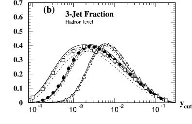
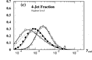
Figure 5: 3- and 4-jet production rates with the Durham algorithm measured by JADE at $\sqrt{s}=35$ GeV (triangles) and OPAL at $\sqrt{s}=91$ GeV (points) and 189 GeV (squares) [177]. The data are corrected for experimental effects. The predictions by Monte Carlo models are indicated by the lines for PYTHIA (solid), HERWIG (dashed), ARIADNE (dotted) and COJETS (dash-dotted).

While the jet production rates are generally well described by the usual Monte Carlo event generators it has been observed that the detailed kinematics of 4-jet events are not always successfully modelled [180, 181, 182]. The kinematics of 4-jet events are studied using angular correlations between the jets, e.g. the Bengtsson-Zerwas angle [183] $\chi_{\mathrm{BZ}}=\angle([\vec{p}_{1}\times\vec{p}_{2}],[\vec{p}_{3}\times\vec{p}_{4}])$, where the $\vec{p}_{i}$, $i=1\ldots 4$ are the momentum vectors of the four jets after energy ordering. Comparing LEP 1 data with simulations showed deviations of up to about 20% while the data can be well described by LO ($\mathcal{O}(\alpha_{\mathrm{S}}^{2})$) or NLO ($\mathcal{O}(\alpha_{\mathrm{S}}^{3})$) calculations corrected for hadronisation effects [184, 180, 185, 181].

The jet structure of hadronic events in $\mathrm{e^{+}e^{-}}$ annihilation has also been studied using a cone based algorithm as commonly used at hadron colliders [186, 177]. An advantage of this study is that the properties of the jets may be compared more directly to results from hadron collider experiments.

4.2 Event shape observables

The event shape observables avoid direct association of particles to jets and calculate instead a single number which classifies the event according to its jet topology. Generally the observables are constructed such that a value of zero corresponds to an ideal 2-jet event consisting of only two back-to-back particles, a small value corresponds to a realistic 2-jet event while increasingly larger values indicate the presence of one or more additional jets. A large number of event shape observables have been proposed and studied. We will concentrate here on observables which are infrared and collinear safe and which have the most complete QCD predictions including contributions from resummed NLLA calculations.

Thrust $T$, Thrust major and minor $T_{\mathrm{maj.}}$ and $T_{\mathrm{min.}}$:

These observables are defined by the expression [187, 188]

$$T=\max_{\vec{n}}\left(\frac{\sum_{i}|\vec{p}_{i}\cdot\vec{n}|}{\sum_{i}|\vec{p}_{i}|}\right)\;\;\;.$$ (36)

where $\vec{p}_{i}$ is the momentum of particle $i$ in an event. The thrust axis $\vec{n}_{T}$ is the vector $\vec{n}$ which maximizes the expression in parentheses. A plane through the origin and perpendicular to $\vec{n}_{T}$ divides the event into two hemispheres $H_{1}$ and $H_{2}$. A value of $T=1$ corresponds to an ideal 2-jet event; therefore the thrust observable is often used in the form $1-T$. Based on the thrust axis $\vec{n}_{T}$ the thrust major $T_{\mathrm{maj.}}$ and the thrust major axis $\vec{n}_{T_{\mathrm{maj.}}}$ are defined by equation (36) with the constraint $\vec{n}_{T}\cdot\vec{n}=0$. The thrust minor $T_{\mathrm{min.}}$ and the thrust minor axis $\vec{n}_{T_{\mathrm{min.}}}$ are defined by the expression in parenthesis of equation (36) with the constraint $[\vec{n}_{T}\times\vec{n}_{T_{\mathrm{maj.}}}]=\vec{n}_{T_{\mathrm{min.}}}$.

Heavy and Light Jet Mass $M_{H}$ and $M_{L}$:

The hemisphere invariant masses are calculated using the particles in the two hemispheres $H_{1}$ and $H_{2}$. We define $M_{H}$ [189, 190] as the heavier mass and $M_{L}$ as the lighter mass, both normalised to $\sqrt{s}$.

C- and D-parameter $C$ and $D$:

The linearised momentum tensor $\Theta^{\alpha\beta}$ is defined by

$$\Theta^{\alpha\beta}=\frac{\sum_{i}(p_{i}^{\alpha}p_{i}^{\beta})/|\vec{p}_{i}|}{\sum_{i}|\vec{p}_{i}|}\;\;\;,\;\;\;\alpha,\beta=1,2,3\;\;\;.$$

The three eigenvalues $\lambda_{j}$ of this tensor define $C$ [22] through

$$C=3(\lambda_{1}\lambda_{2}+\lambda_{2}\lambda_{3}+\lambda_{3}\lambda_{1})\;\;.$$

An equivalent and numerically more convenient form is [35]

$$C=\frac{3}{2}\frac{\sum_{ij}|\vec{p}_{i}||\vec{p}_{j}|\sin^{2}\theta_{ij}}{(\sum_{i}|\vec{p}_{i}|)^{2}}$$

where $\theta_{ij}$ is the angle between particles $i$ and $j$. The D-parameter is defined by

$$D=27\lambda_{1}\lambda_{2}\lambda_{3}\;\;\;.$$

Jet Broadening observables $B_{T}$, $B_{W}$ and $B_{N}$:

These are defined by computing the quantity

$$B_{k}=\left(\frac{\sum_{i\in H_{k}}|\vec{p}_{i}\times\vec{n}_{T}|}{2\sum_{i}|\vec{p}_{i}|}\right)$$

for each of the two event hemispheres, $H_{k}$, defined above. The three observables [191] are defined by

$$B_{T}=B_{1}+B_{2},\;\;\;B_{W}=\max(B_{1},B_{2})\;\;\;\mathrm{and}\;\;\;B_{N}=\min(B_{1},B_{2})$$

where $B_{T}$ is the total, $B_{W}$ is the wide and $B_{N}$ is the narrow jet broadening.

Transition value between 2 and 3 jets $y_{23}^{\mathrm{D}}$:

The Durham jet algorithm (see section 4.1) is applied to cluster the particles of an hadronic event into two or three jets. The value of $y_{\mathrm{cut}}$ at which for an event the transition between a 2-jet and a 3-jet assignment occurs is called $y_{23}^{\mathrm{D}}$ [173].

We will refer to event shape observables in general by the symbol $y$. The observables $T_{\mathrm{min.}}$, $M_{L}$, $D$ and $B_{N}$ belong to the class of 4-jet observables, because for these we have in the cms $y>0$ only for events with at least four partons in the final state. We also note that some of the observables take the whole event into account while others depend only on one selected hemisphere of the event; the observables $M_{H}$, $M_{L}$, $B_{W}$, $B_{N}$ and $y_{23}^{\mathrm{D}}$ fall into the latter category.

Figure 6 presents measurements by OPAL at average $\sqrt{s}=91,133,177$ and 197 GeV of the event shape observables $y_{23}^{\mathrm{D}}$ (left) and $D$ (right) representing 3- and 4-jet observables [182]. The data are corrected for experimental effects and compared to predictions by Monte Carlo models. One finds that the data for $y_{23}^{\mathrm{D}}$ are well described by the models at all energies. The data for $D$ are also well described by the models at high energies $\sqrt{s}>m_{\mathrm{Z^{0}}}$ where the statistical and experimental errors are comparatively large. However, at $\sqrt{s}=91$ GeV and large values of $D$ significant deviations between models and data occur; for HERWIG there are also discrepancies at $D\approx 10^{-2}$. This observation could be related to the unsuccessful modelling of the kinematics of 4-jet events discussed above.

Figure 6: Distributions of event shape observables $y_{23}^{\mathrm{D}}$ (left) and $D$ (right) measured by OPAL [182]. The data are corrected for experimental effects. The high energy LEP 2 data collected at several energy points are combined into two samples at average $\sqrt{s}=177$ and 197 GeV. The data sets are separated vertically by multiplicative factors as indicated for clarity. The lines show the predictions of Monte Carlo models as indicated on the figures. The lower parts of the figures present the deviations between data and Monte Carlo model predictions at $\sqrt{s}=91$ and 197 GeV.

Another way of studying the structure of hadronic events in $\mathrm{e^{+}e^{-}}$ annihilation is to calculate moments of the event shape observable distributions:

$$\mbox{$\langle y^{n}\rangle$}=\int_{0}^{y_{\mathrm{max}}}y^{n}\frac{1}{\sigma}\frac{\mathrm{d}\sigma}{\mathrm{d}y}\mathrm{d}y\;,$$

where $y_{\mathrm{max}}$ is the maximal kinematically allowed value of the observable. The moments always sample all of the available phase space with a different weighting depending on the value of $n$; moments with small values of $n$ are dominated by 2- and 3-jet events while for larger values of $n$ multi-jet events become more important. Figure 7 (left) shows the first five moments of the observables $1-T$, $M_{H}$ and $C$ measured by OPAL [182] at $\sqrt{s}=91$ to 197 GeV. The data are compared to predictions by Monte Carlo models and good agreement is found, except for HERWIG which shows deviations from the moments of $1-T$ and $C$ increasing with $n$.

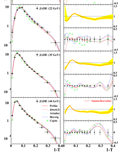
Figure 7: (left) Moments $n=1,\ldots,5$ of event shape observables $1-T$, $M_{H}$ and $C$ measured by OPAL [182]. The data are corrected for experimental effects. The lines show the predictions by Monte Carlo models as indicated. The lower parts of the figure present the deviations between data and Monte Carlo models at $\sqrt{s}=91$ and 197 GeV. (right) Distributions of $1-T$ measured using JADE data and corrected for experimental effects at $\sqrt{s}$=14 to 44 GeV [192, 193]. The lines or crosses show predictions by Monte Carlo models as indicated. The set of figures on the RHS present the correction factors $K_{i}$ (lines) and their uncertainties (shaded bands), and the differences $\delta_{i}$ between data and Monte Carlo model predictions together with the errors of the data.

The reanalysis of data from the JADE experiment made it possible to compare data for event shape observables at $\sqrt{s}<m_{\mathrm{Z^{0}}}$ with the predictions of current Monte Carlo models [192, 193]. Figure 7 (right) presents as an example measurements of distributions of $1-T$ at $\sqrt{s}=14$, 22, 35 and 44 GeV. The data from the JADE experiment are corrected for experimental effects and the presence of $\mathrm{e^{+}e^{-}}\rightarrow\mathrm{b\overline{b}}$ events corresponding to about 9% of the event samples. The predictions of Monte Carlo models tuned by OPAL to LEP 1 data are superimposed and found to agree well with the data; the exception is COJETS which deviates from the data in particular at low $\sqrt{s}$.

4.3 Experimental tests of asymptotic freedom

Jet rates and event shape observables are well suited to investigate experimentally one of the most important predictions of QCD, namely asymptotic freedom of the strong coupling, see sections 2 and 3. The large range in cms energies $\sqrt{s}$ provided by the LEP data and also the earlier data from previous $\mathrm{e^{+}e^{-}}$ colliders gives direct access to effects caused by the running strong coupling constant.

Following earlier studies [160, 161] the L3 collaboration measured the fraction of 3-jet events using the JADE E0 algorithm at $y_{\mathrm{cut}}=0.08$ [72]. This measurement is especially suited to study asymptotic freedom, since the hadronisation corrections as predicted by Monte Carlo models are known to be small (less than 10%) and fairly model independent [170, 168]. The L3 data and results from other experiments spanning the range $\sqrt{s}=22$ to 206 GeV are shown in figure 8 (left) and compared with the $\mathcal{O}(\alpha_{\mathrm{S}}^{2})$ perturbative QCD expectation with $\alpha_{\mathrm{S}}(m_{\mathrm{Z^{0}}})=0.12$. The prediction clearly agrees with the data.

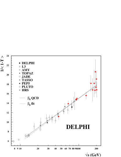
Figure 8: 3-jet fraction $f_{3}$ with the JADE E0 algorithm at $y_{\mathrm{cut}}=0.08$ (left) and $1/\mbox{$\langle 1-T\rangle$}$ (right) measured as a function of the cms energy [72, 194]. The data are compared with predictions by QCD shown by the solid lines.

Figure 8 (right) presents the results of a similar analysis by DELPHI [194] using the mean values $\langle 1-T\rangle$ of the $1-T$ distributions measured at energies ranging from below 10 GeV to 202 GeV. The figure shows the quantity $1/\mbox{$\langle 1-T\rangle$}$ vs. $\sqrt{s}$ on a logarithmic scale, because from equations (7) and (16) a logarithmic dependence in LO is predicted. This prediction is well confirmed by the data. The solid line shows the QCD prediction in NLO in a special formulation independent of a particular renormalisation scheme [14, 195] (see section 4.5.2) which is also seen to suppress non-perturbative effects.

4.4 Measurements of $\alpha_{\mathrm{S}}$

4.4.1 3-jet observables

Early measurements of $\alpha_{\mathrm{S}}$ before the start of LEP using event shape or jet observables were briefly summarised in section 3. The first analyses by the LEP collaborations used $\mathcal{O}(\alpha_{\mathrm{S}}^{2})$ QCD calculations and already a set of Monte Carlo event generators including QCD coherence effects and tuned to the precise LEP data, see e.g. [175] for a review. An average value of $\alpha_{\mathrm{S}}(m_{\mathrm{Z^{0}}})=0.120\pm 0.006$ was determined, where the error is dominated by theoretical uncertainties estimated by variation of the renormalisation scale in the QCD calculations. Compared to the earlier determinations of $\alpha_{\mathrm{S}}(m_{\mathrm{Z^{0}}})$ the error of the combined LEP measurements was reduced by a factor of more than two. This improvement was mostly due to the use of consistent hadronisation models as well as reliable $\mathcal{O}(\alpha_{\mathrm{S}}^{2})$ QCD calculations [23]. The error was also seen to be consistent with the scatter of results from individual observables; this is an important cross-check of the methods for estimating the errors. A reanalysis of low energy data at $\sqrt{s}=35$ GeV from the JADE experiment using the methods developed for LEP obtained $\alpha_{\mathrm{S}}(m_{\mathrm{Z^{0}}})=0.122^{+0.008}_{-0.005}$ consistent with the LEP result [196].

A significant improvement in the determinations of $\alpha_{\mathrm{S}}$ based on event shape or jet observables was the introduction of resummed calculations matched to the fixed order predictions ($\mathcal{O}(\alpha_{\mathrm{S}}^{2})$+NLLA) discussed in section 2. These calculations allow the data to be described over larger regions of phase space in the 2-jet region and have generally a weaker dependence on the renormalisation scale [34]. A combination of values of $\alpha_{\mathrm{S}}(m_{\mathrm{Z^{0}}})$ obtained from analyses at $\sqrt{s}\approx m_{\mathrm{Z^{0}}}$ using $\mathcal{O}(\alpha_{\mathrm{S}}^{2})$+NLLA calculations was given in [197] as $\alpha_{\mathrm{S}}(m_{\mathrm{Z^{0}}})=0.121\pm 0.006$. Thus the total error was not improved compared to $\mathcal{O}(\alpha_{\mathrm{S}}^{2})$ based analyses but the result is considered to be more reliable theoretically due to the reduced dependence on the renormalisation scale.

Recently the LEP experiments have published their final results on determinations of $\alpha_{\mathrm{S}}$ based on data at $\sqrt{s}=m_{\mathrm{Z^{0}}}$ up to the highest LEP 2 energies [178, 198, 72, 182]. These analyses use a consistent set of observables: $1-T$, $M_{H}$, $B_{T}$, $B_{W}$ and $C$ and in addition $y_{23}^{\mathrm{D}}$ by ALEPH and OPAL. All analyses employ the most recent calculations for the resummed NLLA calculations [30, 32, 33, 31] and the modified $\ln(R)$-matching scheme and thus the results may be compared directly.

Figure 9 (left) shows as a representative example the results of the analysis by ALEPH using the observable $B_{T}$ at $\sqrt{s}=91.2$ to 206 GeV [178]. The data are corrected for experimental effects and the curves present the $\mathcal{O}(\alpha_{\mathrm{S}}^{2})$+NLLA QCD prediction using the modified $\ln(R)$-matching corrected for hadronisation. The fits have been performed over ranges indicated by the solid lines while the dashed lines are an extrapolation of the theory using the fitted results. The agreement between the theory including hadronisation corrections and the data is good in the fitted regions and becomes worse in the extreme 2-jet and multijet regions where the theory is not expected to be able to completely describe the data.

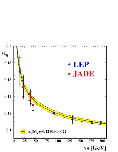
Figure 9: (left) Distributions of $B_{T}$ measured by ALEPH at several energy points as indicated [178]. Superimposed are fits of the QCD prediction corrected for hadronisation effects. The fits have been performed in the ranges shown by the solid lines while the dashed lines show an extrapolation of the fitted predictions. (right) Combined values of $\alpha_{\mathrm{S}}$ based on the analyses by the LEP experiments or using JADE data (see text) are shown. The total (inner) errors bars show total (experimental) uncertainties. The lines and shaded band show the evolution of $\alpha_{\mathrm{S}}$ based on the value of $\alpha_{\mathrm{S}}(m_{\mathrm{Z^{0}}})$ given on the figure.

In order to study asymptotic freedom the individual results on $\alpha_{\mathrm{S}}$ from the most recent LEP analyses [178, 198, 72, 182] are combined using a common method, see e.g. [178, 182, 199, 200]. The values of $\alpha_{\mathrm{S}}$ to be combined are evolved to the common scale of the combination if necessary. Then the average value $\bar{\alpha}_{\mathrm{S}}$ is computed by minimising

$$\chi^{2}=(\vec{\alpha}-\bar{\alpha}_{\mathrm{S}})\cdot V^{-1}\cdot(\vec{\alpha}-\bar{\alpha}_{\mathrm{S}})^{T}$$ (37)

w.r.t. to $\bar{\alpha}_{\mathrm{S}}$. The individual measurements ${\alpha_{\mathrm{S}}}_{,i}$ are collected in the vector $\vec{\alpha}$ and $V$ is the covariance matrix of the measurements. The final expression for the average value is

$$\bar{\alpha}_{\mathrm{S}}=\sum_{i}w_{i}{\alpha_{\mathrm{S}}}_{,i}\,,\;w_{i}=\frac{\sum_{j}(V^{-1})_{ij}}{\sum_{j,k}(V^{-1})_{jk}}\;\;.$$ (38)

The correlations between experimental, hadronisation and theoretical uncertainties are generally not well known, in particular between different experiments, and thus models for the correlations have to be constructed. In these models three levels of correlation $\rho_{ij}$ between the errors $\sigma_{i}$ and $\sigma_{j}$ of two measurements $i$ and $j$ may be assumed: i) no correlations $\rho_{ij}=0$, ii) partial correlation $\rho_{ij}=\min(\sigma_{i},\sigma_{j})^{2}/(\sigma_{i}\sigma_{j})$ or iii) full correlation $\rho_{ij}=1$. The treatment of the different systematic uncertainties is as follows:

Experimental uncertainties

These are added to the diagonal and off-diagonal elements of $V$ using one of the three possible models for their correlation.

Hadronisation uncertainties

These are added only to the diagonal elements of $V$. The hadronisation uncertainty is evaluated by repeating the combination with individual ${\alpha_{\mathrm{S}}}_{,i}$ values obtained with different hadronisation models.

Theoretical uncertainties

These are also added only to the diagonal elements of $V$. The theoretical uncertainty is evaluated by varying all individual values ${\alpha_{\mathrm{S}}}_{,i}$ simultaneously within their theoretical uncertainties and repeating the combination.

This procedure suppresses the presence of negative weights $w_{i}$ which otherwise appear when large off-diagonal terms are included in $V$ [200]. Such negative weights are mathematically correct but difficult to interpret as a physical result. We therefore choose a treatment of the correlations of the generally large hadronisation and theoretical uncertainties which avoids negative weights as in [178, 182].

In a first step the individual results for each observable and experiment are combined in the energy ranges $130\leq\sqrt{s}\leq 136$ GeV, $161\leq\sqrt{s}\leq 183$ GeV and $189\leq\sqrt{s}\leq 207$ GeV corresponding to average centre-of-mass energies $\sqrt{s}=133,177$ and 197 GeV. In these combinations the statistical errors are taken as uncorrelated and the experimental errors as partially correlated. OPAL publishes results directly at $\sqrt{s}=177$ and 197 GeV and also at points from smaller energy ranges. Our averages reproduce the OPAL results within 1% and with consistent uncertainties. The single DELPHI result from $\sqrt{s}=183$ GeV is simply evolved to 177 GeV.

The sets of results for each observable and experiment are further combined within each experiment. The statistical correlations between observables as obtained by ALEPH and OPAL at $\sqrt{s}=206$ GeV are taken from [200]. The experimental uncertainties are again taken as partially correlated. Our values for $\alpha_{\mathrm{S}}$ are shown in table 4. The corresponding combined results from OPAL have been calculated using the same method except for a more detailed treatment of hadronisation uncertainties. Our combined results again reproduce the OPAL results within 1% with consistent errors.

Table 4: Results for average values of $\alpha_{\mathrm{S}}$ from LEP experiments [178, 198, 72, 182]. The columns show the results for $\alpha_{\mathrm{S}}(\sqrt{s})$, the statistical (stat.), experimental (exp.), hadronisation (had.) and theoretical (theo.) uncertainties. The last two rows give average values of $\alpha_{\mathrm{S}}(m_{\mathrm{Z^{0}}})$ of all LEP 2 data from $\sqrt{s}=133$ to 197 GeV and of all LEP data.

• 	$\alpha_{\mathrm{S}}(m_{\mathrm{Z^{0}}})$ $\pm$	stat. $\pm$	exp. $\pm$	had. $\pm$	theo.
  ALEPH	0.1201 $\pm$	0.0002 $\pm$	0.0007 $\pm$	0.0020 $\pm$	0.0050
  DELPHI	0.1216 $\pm$	0.0002 $\pm$	0.0021 $\pm$	0.0024 $\pm$	0.0056
  L3	0.1211 $\pm$	0.0008 $\pm$	0.0014 $\pm$	0.0035 $\pm$	0.0050
  OPAL	0.1193 $\pm$	0.0002 $\pm$	0.0007 $\pm$	0.0024 $\pm$	0.0047
  LEP	0.1204 $\pm$	0.0002 $\pm$	0.0006 $\pm$	0.0025 $\pm$	0.0051
  	$\alpha_{\mathrm{S}}$(133 GeV) $\pm$	stat. $\pm$	exp. $\pm$	had. $\pm$	theo.
  ALEPH	0.1156 $\pm$	0.0028 $\pm$	0.0008 $\pm$	0.0014 $\pm$	0.0048
  L3	0.1133 $\pm$	0.0023 $\pm$	0.0018 $\pm$	0.0024 $\pm$	0.0048
  OPAL	0.1091 $\pm$	0.0033 $\pm$	0.0033 $\pm$	0.0016 $\pm$	0.0036
  LEP	0.1124 $\pm$	0.0017 $\pm$	0.0011 $\pm$	0.0018 $\pm$	0.0043
  	$\alpha_{\mathrm{S}}$(177 GeV) $\pm$	stat. $\pm$	exp. $\pm$	had. $\pm$	theo.
  ALEPH	0.1106 $\pm$	0.0024 $\pm$	0.0008 $\pm$	0.0010 $\pm$	0.0040
  DELPHI	0.1093 $\pm$	0.0035 $\pm$	0.0020 $\pm$	0.0017 $\pm$	0.0043
  L3	0.1077 $\pm$	0.0020 $\pm$	0.0014 $\pm$	0.0018 $\pm$	0.0045
  OPAL	0.1074 $\pm$	0.0010 $\pm$	0.0011 $\pm$	0.0009 $\pm$	0.0032
  LEP	0.1081 $\pm$	0.0013 $\pm$	0.0009 $\pm$	0.0013 $\pm$	0.0040
  	$\alpha_{\mathrm{S}}$(197 GeV) $\pm$	stat. $\pm$	exp. $\pm$	had. $\pm$	theo.
  ALEPH	0.1075 $\pm$	0.0012 $\pm$	0.0009 $\pm$	0.0008 $\pm$	0.0036
  DELPHI	0.1083 $\pm$	0.0013 $\pm$	0.0021 $\pm$	0.0017 $\pm$	0.0042
  L3	0.1124 $\pm$	0.0007 $\pm$	0.0013 $\pm$	0.0014 $\pm$	0.0046
  OPAL	0.1074 $\pm$	0.0010 $\pm$	0.0011 $\pm$	0.0009 $\pm$	0.0032
  LEP	0.1085 $\pm$	0.0006 $\pm$	0.0007 $\pm$	0.0011 $\pm$	0.0038
  	$\alpha_{\mathrm{S}}(m_{\mathrm{Z^{0}}})$ $\pm$	stat. $\pm$	exp. $\pm$	had. $\pm$	theo.
  LEP 2	0.1200 $\pm$	0.0007 $\pm$	0.0010 $\pm$	0.0016 $\pm$	0.0048
  LEP all	0.1201 $\pm$	0.0005 $\pm$	0.0008 $\pm$	0.0019 $\pm$	0.0049

Applying the same procedure to the reanalysed data from the JADE experiment collected at $\sqrt{s}=14$ to 44 GeV [201] yields the results shown in table 5. The analysis of the JADE data was performed using the same event shape observables, QCD calculations and essentially the same Monte Carlo programs to calculate the hadronisation corrections as for the LEP analyses and therefore the results may be compared directly.

Table 5: Results for average values of $\alpha_{\mathrm{S}}$ from JADE. The last row gives the average value of $\alpha_{\mathrm{S}}(m_{\mathrm{Z^{0}}})$ from all JADE data.

• $\sqrt{s}$	$\alpha_{\mathrm{S}}(\sqrt{s})$ $\pm$	stat. $\pm$	exp. $\pm$	had. $\pm$	theo.
  14	0.1704 $\pm$	0.0044 $\pm$	0.0041 $\pm$	0.0148 $\pm$	0.0117
  22	0.1514 $\pm$	0.0040 $\pm$	0.0030 $\pm$	0.0106 $\pm$	0.0084
  35	0.1430 $\pm$	0.0010 $\pm$	0.0022 $\pm$	0.0076 $\pm$	0.0079
  38	0.1388 $\pm$	0.0035 $\pm$	0.0030 $\pm$	0.0056 $\pm$	0.0070
  44	0.1299 $\pm$	0.0020 $\pm$	0.0031 $\pm$	0.0057 $\pm$	0.0057
  	$\alpha_{\mathrm{S}}(m_{\mathrm{Z^{0}}})$ $\pm$	stat. $\pm$	exp. $\pm$	had. $\pm$	theo.
  JADE	0.1203 $\pm$	0.0007 $\pm$	0.0017 $\pm$	0.0053 $\pm$	0.0050

The average values of $\alpha_{\mathrm{S}}$ determined at each $\sqrt{s}$ as shown in tables 4 and 5 are presented in figure 9 (right). The data are compared with the QCD prediction for the running of $\alpha_{\mathrm{S}}$ calculated in NNLO based on the average value $\alpha_{\mathrm{S}}(m_{\mathrm{Z^{0}}})=0.1211\pm 0.0021$ (see section 7) which has been determined using only NNLO QCD calculations. The agreement with the data is excellent and provides strong evidence for asymptotic freedom.

Measurements of the first five moments of the six event shape observables discussed above and as shown partially in figure 7 (left) have been used by OPAL to determine the strong coupling constant using only NLO ($\mathcal{O}(\alpha_{\mathrm{S}}^{2})$) QCD predictions [182]. The NLLA predictions break down at very small values of the observables $y\ll 1$ and also become unreliable close to the kinematic limits $y_{\mathrm{max}}$ and thus cannot be used to derive moments. The divergences of the NLO predictions for $y\rightarrow 0$ are not a problem, since these are integrable and stable predictions for the moments are obtained. After demanding that the ratio of the NLO to the LO terms in the perturbative QCD predictions be less than 0.5 results from 17 observables are considered: $\langle 1-T\rangle$, $\langle C\rangle$, $\langle B_{T}\rangle$, $\langle B_{W}^{n}\rangle$ and $\langle y_{23}^{n}\rangle$ with $n=1,\ldots,5$, and $\langle M_{H}^{n}\rangle$ with $n=2,\ldots,5$. The final combined result is $\alpha_{\mathrm{S}}(m_{\mathrm{Z^{0}}})=0.1223\pm 0.0005\mathrm{(stat.)}\pm 0.0014\mathrm{(exp.)}\pm 0.0016\mathrm{(had.)}^{+0.0054}_{-0.0036}\mathrm{(theo.)}$ in good agreement with the results from distributions discussed above. This analysis constitutes a valuable cross check of the determination of $\alpha_{\mathrm{S}}$ from 3-jet observables, since with moments the complete phase space is used.

4.4.2 4-jet observables

The study of 4-jet observables for measurements of $\alpha_{\mathrm{S}}(m_{\mathrm{Z^{0}}})$ is promising, because the sensitivity of these observables to the strong coupling is doubled compared to 3-jet observables. The relative change in $\alpha_{\mathrm{S}}$ induced by a change of a 3-jet observable $O_{3}\sim\alpha_{\mathrm{S}}$ is given by $\Delta\alpha_{\mathrm{S}}/\alpha_{\mathrm{S}}=\Delta O_{3}/O_{3}$ while for a 4-jet observable $O_{4}\sim\alpha_{\mathrm{S}}^{2}$ we have $\Delta\alpha_{\mathrm{S}}/\alpha_{\mathrm{S}}=\Delta O_{4}/(2O_{4})$.

The ALEPH collaboration has performed a measurement of $\alpha_{\mathrm{S}}(m_{\mathrm{Z^{0}}})$ using the fraction of 4-jet events $\mathrm{R}_{4}$ determined using the Durham algorithm in hadronic $\mathrm{Z^{0}}$ decays [181]. The QCD prediction is known in $\mathcal{O}(\alpha_{\mathrm{S}}^{3})$, i.e.  LO is $\mathcal{O}(\alpha_{\mathrm{S}}^{2})$ and NLO radiative corrections are $\mathcal{O}(\alpha_{\mathrm{S}}^{3})$ [202, 28]. These calculations are matched with existing NLLA calculations.

The measurement of $\alpha_{\mathrm{S}}(m_{\mathrm{Z^{0}}})$ based on these predictions is presented in figure 10 [181]. The uncorrected data for $\mathrm{R}_{4}$ measured with $2.5\cdot 10^{6}$ hadronic $\mathrm{Z^{0}}$ decays using the Durham algorithm are shown as a function of the jet resolution parameter $y_{\mathrm{cut}}$. The line shows the fit of the $\mathcal{O}(\alpha_{\mathrm{S}}^{3})$+NLLA (R-matching) theory corrected for hadronisation and detector effects. The fit is performed using only the bins within the fit range as indicated where the total correction factors deviate from unity by less than 10%. The result of the fit for fixed renormalisation scale parameter $x_{\mu}=1$ is $\alpha_{\mathrm{S}}(m_{\mathrm{Z^{0}}})=0.1170\pm 0.0001\mathrm{(stat.)}\pm 0.0022\mathrm{(syst.)}$ using the conservatively estimated systematic uncertainty from [181]. The systematic error has contributions from experimental ($\pm 0.0009$), hadronisation ($\pm 0.0010$) and theoretical ($\pm 0.0017$) uncertainties and the fit is seen to describe the precise data fairly well.

A similar analysis by DELPHI [203] uses only the $\mathcal{O}(\alpha_{\mathrm{S}}^{3})$ (NLO) calculations with experimentally optimised renormalisation scale and finds $\alpha_{\mathrm{S}}(m_{\mathrm{Z^{0}}})=0.1175\pm 0.0005\mathrm{(stat.)}\pm 0.0010\mathrm{(exp.)}\pm 0.0027\mathrm{(had.)}\pm 0.0007\mathrm{(theo.)}$ with $x_{\mu}=0.042$ for the closely related Cambridge algorithm [171] and $\alpha_{\mathrm{S}}(m_{\mathrm{Z^{0}}})=0.1178\pm 0.0036$ with $x_{\mu}=0.015$ for the Durham algorithm. A study from OPAL using $\mathrm{R}_{4}$ measured with LEP 1 and LEP 2 data found $\alpha_{\mathrm{S}}(m_{\mathrm{Z^{0}}})=0.1182\pm 0.0003\mathrm{(stat.)}\pm 0.0015\mathrm{(exp.)}\pm 0.0011\mathrm{(had.)}\pm 0.0018\mathrm{(theo.)}$ [204]. Measurements of $\mathrm{R}_{4}$ with JADE data at $\sqrt{s}$ between 14 and 44 GeV found as a preliminary result $\alpha_{\mathrm{S}}(m_{\mathrm{Z^{0}}})=0.1169\pm 0.0004\mathrm{(stat.)}\pm 0.0012\mathrm{(exp.)}\pm 0.0021\mathrm{(had.)}\pm 0.0007\mathrm{(theo.)}$ [205]. The various measurements are in good agreement with each other. All measurements using $\mathrm{R}_{4}$ discussed in this section have comparatively small uncertainties and belong to the group of the most precise determinations of $\alpha_{\mathrm{S}}$.

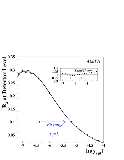
Figure 10: The 4-jet fraction $\mathrm{R}_{4}$ determined using the Durham algorithm is shown as a function of $y_{\mathrm{cut}}$ without corrections. Superimposed is a fit of $\mathcal{O}(\alpha_{\mathrm{S}}^{3})$+NLLA QCD (solid line) corrected for hadronisation and detector effects [181].

4.5 Alternative approaches to soft and hard QCD

4.5.1 Tests of power corrections

Distributions and mean values of event shape observables measured in $\mathrm{e^{+}e^{-}}$ annihilation at many cms energy points between around 14 and more than 200 GeV have been used recently by several groups to study power corrections [206, 194, 198, 178, 72]. In all of these studies pQCD predictions in $\mathcal{O}(\alpha_{\mathrm{S}}^{2})$+NLLA are used for event shape distributions. For the mean values only NLO ($\mathcal{O}(\alpha_{\mathrm{S}}^{2})$) predictions are employed as explained in section 4.4.1. The pQCD predictions are added together in both cases with the power correction predictions. The resulting expressions are functions of the strong coupling $\alpha_{\mathrm{S}}(m_{\mathrm{Z^{0}}})$ and of the non-perturbative parameter $\alpha_{0}$. The complete predictions are compared with data for event shape distributions or mean values corrected for experimental effects. For the mean value of the 4-jet observable D-parameter power correction predictions have been tested as well [72].

Figure 11: (left) Distributions of $1-T$. The vertical axis has arbitrary units and the data points have been scaled for clarity. The solid lines show the result of the fit of the combined pQCD and power correction prediction. The dotted lines represent an extrapolation of the result [206]. (right) Cms energy dependence of the mean values of several event shape observables. The solid lines show the result of the fit of combined $\mathcal{O}(\alpha_{\mathrm{S}}^{2})$ QCD calculations with power corrections while the dashed lines indicate results obtained with Monte Carlo based corrections [178].

Figure 11 (left) shows the results of fitting the data for $1-T$ distributions measured at cms energies from 14 to 189 GeV. The data from experiments at $\sqrt{s}<m_{\mathrm{Z^{0}}}$ are corrected for the effects of $\mathrm{e^{+}e^{-}}\rightarrow\mathrm{b\overline{b}}$ events [206]. The data in the fitted regions are well reproduced by the theory (solid lines). The dotted lines present extrapolations outside of the fitted regions using the fit results for $\alpha_{\mathrm{S}}(m_{\mathrm{Z^{0}}})$ and $\alpha_{0}(2~{}\mathrm{GeV})$ which describe the data reasonably well. The agreement between theory and experiment is similar for other observables.

Figure 11 (right) presents as solid lines the results of fits to measurements of mean values of various event shape observables at $\sqrt{s}=12$ to 206 GeV [178]. The data are well described by the fitted theory. The dotted lines show the results of fits where the power corrections have been replaced by corrections derived from Monte Carlo simulations. The Monte Carlo corrections lead to slighty different theoretical predictions.

Table 6 collects averaged results for $\alpha_{\mathrm{S}}(m_{\mathrm{Z^{0}}})$ and $\alpha_{0}(2~{}\mathrm{GeV})$ from the various analyses [206, 178, 194, 72]. The averages are as given by the authors and are based upon differing sets of observables, definitions of systematic uncertainties and averaging methods. It is therefore not useful to compute global averages from these results. There is good agreement between the various analyses of mean values or distributions of event shape observables.

Table 6: Results of power correction analysis using the DMW model.

• 		ALEPH [178]	DELPHI [194]	L3 [72]	[206]
  	$\alpha_{\mathrm{S}}(m_{\mathrm{Z^{0}}})$	0.111	0.108	–	0.111
  distri-		$\pm$0.005	$\pm$0.002		$\pm$0.004
  butions	$\alpha_{0}(2~{}\mathrm{GeV})$	0.50	0.55	–	0.58
  		$\pm$0.10	$\pm$0.03		$\pm$0.09
  	$\alpha_{\mathrm{S}}(m_{\mathrm{Z^{0}}})$	–	0.121	0.113	0.119
  mean			$\pm$0.006	$\pm$0.006	$\pm$0.003
  values	$\alpha_{0}(2~{}\mathrm{GeV})$	–	0.47	0.48	0.49
  			$\pm$0.08	$\pm$0.06	$\pm$0.06

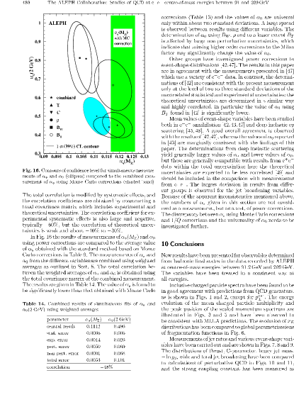
Figure 12: Summaries of results for $\alpha_{\mathrm{S}}(m_{\mathrm{Z^{0}}})$ and $\alpha_{0}(2~{}\mathrm{GeV})$ for distributions (left) [178] and mean values (right) [72]. The error ellipses show one standard deviation uncertainties (39% CL). The shaded band on the left plot gives the combined result for $\alpha_{\mathrm{S}}(m_{\mathrm{Z^{0}}})$ using Monte Carlo based corrections from the same analysis. The bands on the right plot give the unweighted averages of $\alpha_{\mathrm{S}}(m_{\mathrm{Z^{0}}})$ and $\alpha_{0}(2~{}\mathrm{GeV})$ shown in this figure.

Figures 12 (left) and (right) give an overview over results from the analysis of distributions [178] (left) and mean values [72] (right). The results are shown as points with one-standard-deviation error ellipses. The results for $\alpha_{\mathrm{S}}(m_{\mathrm{Z^{0}}})$ of fits to distributions are found to be smaller compared to the results of fits to the same data using Monte Carlo based hadronisation corrections; $\alpha_{\mathrm{S}}(m_{\mathrm{Z^{0}}})\simeq 0.111$ compared to $\alpha_{\mathrm{S}}(m_{\mathrm{Z^{0}}})\simeq 0.120$. There are systematic differences between the DMW power correction model and the hadronisation corrections derived from Monte Carlo models leading to differences in the values of $\alpha_{\mathrm{S}}(m_{\mathrm{Z^{0}}})$ of $\Delta\alpha_{\mathrm{S}}(m_{\mathrm{Z^{0}}})\simeq 0.009$ which are significantly larger than the hadronisation uncertainties quoted in section 4.4.1 as derived from the published results. In the analysis by ALEPH [178] a direct comparison is made using the same data and a consistent average relative difference $\Delta\alpha_{\mathrm{S}}(m_{\mathrm{Z^{0}}})/\alpha_{\mathrm{S}}(m_{\mathrm{Z^{0}}})\simeq 10$% is found. The results for $\alpha_{0}(2~{}\mathrm{GeV})$ from $\rho=M_{H}^{2}$, $B_{W}$ and $B_{T}$ are fairly large compared to the averages. For the observable $M_{H}$ this effect stems from neglecting particle masses [76, 194].

Figure 13: The figure shows a summary of results for $\alpha_{\mathrm{S}}(m_{\mathrm{Z^{0}}})$ and $\alpha_{0}(2~{}\mathrm{GeV})$ from power correction studies [206, 72, 194, 178]. The results labelled PPTSL are from [206].

Figure 13 shows a summary of results for $\alpha_{\mathrm{S}}(m_{\mathrm{Z^{0}}})$ and $\alpha_{0}(2~{}\mathrm{GeV})$ [206, 72, 194, 178]. One observes reasonable agreement between the individual measurements. The non-perturbative parameter $\alpha_{0}$ appears universal within about 20% as expected [81] while the values for $\alpha_{\mathrm{S}}(m_{\mathrm{Z^{0}}})$ are compatible with world averages, e.g. [207] $\alpha_{\mathrm{S}}(m_{\mathrm{Z^{0}}})=0.1184\pm 0.0027$.

4.5.2 Studies of renormalisation schemes

The ideas about choosing optimal renormalisation schemes (RS) discussed in section 2.1.1 have been tested experimentally. In [197] the predictions for $x_{\mu}$ from the three methods for the hadronic width of the $\mathrm{Z^{0}}$ $R_{\mathrm{Z}}=\Gamma(\mathrm{Z^{0}}\rightarrow\mathrm{hadrons})/\Gamma(\mathrm{Z^{0}}\rightarrow\mathrm{leptons})$ were obtained for NLO QCD. Since for $R_{\mathrm{Z}}$ the QCD prediction is known in NNLO the resulting values of $\alpha_{\mathrm{S}}(m_{\mathrm{Z^{0}}})$ from scale optimized NLO QCD may be compared with the corresponding result from NNLO QCD. It is found that for this observable the three methods agree well, but the resulting value of $\alpha_{\mathrm{S}}(m_{\mathrm{Z^{0}}})$ is significantly lower by $\Delta\alpha_{\mathrm{S}}(m_{\mathrm{Z^{0}}})\simeq 0.003$ compared to the values determined with the NNLO calculations.

In [208] the DELPHI collaboration measured many event shape observables using precise LEP data from the $\mathrm{Z^{0}}$ peak and compared the data to NLO QCD predictions; a similar analysis is discussed in [209]. In fits where the renormalisation scale parameter $x_{\mu}$ and thus effectively the RS was allowed to vary in addition to $\alpha_{\mathrm{S}}(m_{\mathrm{Z^{0}}})$ consistent results within the errors for $\alpha_{\mathrm{S}}(m_{\mathrm{Z^{0}}})$ were found resulting in an unweighted average of $\alpha_{\mathrm{S}}(m_{\mathrm{Z^{0}}})=0.1170\pm 0.0025$ where the error is given by the variance of the set of measurements. Within the fitted ranges of the distributions no evidence for a dependence of $x_{\mu}$ on the observable was found, implying that a single value of $x_{\mu}$ is indeed sufficient. As a comparison the corresponding fits with $x_{\mu}=1$ yielded an unweighted average and variance of $\alpha_{\mathrm{S}}(m_{\mathrm{Z^{0}}})=0.123\pm 0.015$; i.e. not using experimentally optimised scaled results in a significantly increased variance. Similar observations were made in [210]. However, these results are not supported by the findings of [209] where for a similar set of observables as in [208, 210] $\alpha_{\mathrm{S}}(m_{\mathrm{Z^{0}}})=0.127\pm 0.008$ for fits with $x_{\mu}=1$ and $\alpha_{\mathrm{S}}(m_{\mathrm{Z^{0}}})=0.117\pm 0.007$ for fits with $x_{\mu}$ free was observed.

Applying the scale or RS setting methods to fits of limited ranges of distributions is in principle problematic, because more than one energy scale is involved. However, since it is known experimentally that a single value of $x_{\mu}$ is sufficient to describe the data the effects of the additional energy scales introduced by the observable values may be assumed to be small. In [208] the ECH and PMS methods generally lead to similar results for $\alpha_{\mathrm{S}}(m_{\mathrm{Z^{0}}})$, consistent with the theoretical observation that their predictions for the optimal scale are closely related, see e.g. [15]. The resulting values of $\alpha_{\mathrm{S}}(m_{\mathrm{Z^{0}}})$ are also consistent with each other. The weighted averages of the set of observables with the PMS or ECH methods are $\alpha_{\mathrm{S}}(m_{\mathrm{Z^{0}}})=0.115\pm 0.004$ with $\chi^{2}/\mathrm{d.o.f.}\simeq 1$. For the BLM method $\chi^{2}/\mathrm{d.o.f.}=29/13$ is found indicating less consistency among the results. The observation that values of $\alpha_{\mathrm{S}}(m_{\mathrm{Z^{0}}})$ obtained from theoretically optimised RS tend to be smaller than purely experimental values may be explained by noticing that in the PMS method (which is close to the ECH method) a stationary point and usually a minimum of $\alpha_{\mathrm{S}}(m_{\mathrm{Z^{0}}},x_{\mu})$ is chosen as the optimum.

By extending the ECH method it turns out to be possible to relate QCD predictions for different physical observables to each other without explicit dependence on the RS [14, 17, 211]. The QCD prediction for an inclusive observable $R(Q)$ depending on only one energy scale $Q$ is given by the generalised $\beta$-function:

$$Q\frac{\mathrm{d}R}{\mathrm{d}Q}=-bR^{2}(1+\rho_{1}R+\rho_{2}R^{2}+\ldots)=b\rho(R)\;\;.$$ (39)

with $b=2\pi\beta_{0}$. The $\rho_{i}$ are RS independent but can be derived from the corresponding RS dependent coefficients. Equation (39) may be solved analogously to the $\beta$-function of $\alpha_{\mathrm{S}}$ in terms of a process dependent scale parameter $\Lambda_{R}$. Thanks to the Celmaster-Gonsalves relation [212] such parameters for different observables may be related to each other or e.g. to the scale parameter $\Lambda_{\overline{\mathrm{MS}}}$ of the running strong coupling $\alpha_{\mathrm{S}}(\mu)$ in the $\overline{\mathrm{MS}}$ renormalisation scheme:

$$\frac{\Lambda_{R}}{\Lambda_{\overline{\mathrm{MS}}}}=e^{r_{1}/b}\left(\frac{2c_{1}}{b}\right)^{-c_{1}/b}\;\;.$$ (40)

The variables are $c_{1}=2\pi\beta_{1}/\beta_{0}$ and $r_{1}=B_{R}/(2A_{R})$ where $A_{R}$ and $B_{R}$ are the LO and NLO coefficients for the observable calculated in the $\overline{\mathrm{MS}}$ scheme. This procedure may be referred to as renormalisation group improved perturbative QCD (RGI QCD) [10]. Non-perturbative effects scaling like $1/Q$ for most observables may be included with an additional free parameter $K_{0}$ [213].

The DELPHI collaboration has studied mean values of several event shape observables and in addition distributions of the event shape observables EEC and JCEF using the RGI QCD method as explained above [194]. The analysis also uses data from lower energy experiments to cover values of $\sqrt{s}$ from 22 GeV to 200 GeV. The results for $\alpha_{\mathrm{S}}(m_{\mathrm{Z^{0}}})$ from 12 observables are consistent with each other within their uncertainties, as shown in figure 14 (left). The variance of the individual values of $\alpha_{\mathrm{S}}(m_{\mathrm{Z^{0}}})$ is about $\Delta\alpha_{\mathrm{S}}(m_{\mathrm{Z^{0}}})\simeq 0.002$ while the variance of $\alpha_{\mathrm{S}}(m_{\mathrm{Z^{0}}})$ results of corresponding fits based on standard NLO QCD combined with power corrections is observed to be about twice as large. The values of the power correction parameter $K_{0}$ are found to be small and consistent with zero within their uncertainties. Figure 14 (right) shows as examples the results of RGI QCD fits without power corrections, i.e. $K_{0}=0$, for the mean values of $T_{\mathrm{maj.}}$, $1-T$ and $C$.

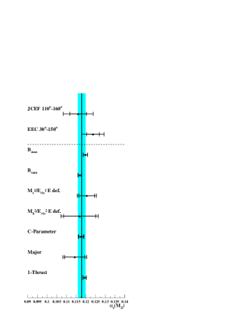
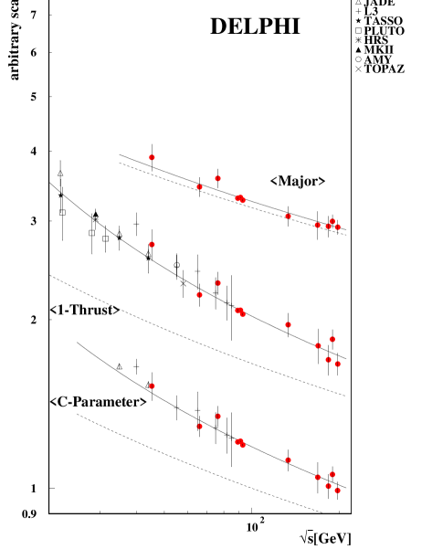
Figure 14: (left) The figure summarises results for $\alpha_{\mathrm{S}}(m_{\mathrm{Z^{0}}})$ from RGI QCD fits with power corrections. The error bars include statistical and experimental systematic uncertainties. The solid lines and grey bands indicate the unweighted mean and variance based on mean values of event shape observables. (right) The figure shows fits of RGI QCD without non-perturbative corrections to mean values of $T_{\mathrm{maj.}}$, $1-T$ and $C$ as functions of $\sqrt{s}$ (full lines). As a comparison the dashed lines present the corresponding prediction in the $\overline{\mathrm{MS}}$ RS [194].

The results of the RGI QCD fits are interpreted to imply that a dominating part of the power corrections or hadronisation corrections in standard NLO QCD fits in the $\overline{\mathrm{MS}}$ RS can be absorbed in the RGI QCD. In [194] a systematic shift in $\alpha_{\mathrm{S}}(m_{\mathrm{Z^{0}}})$ of about 2% between fits of RGI QCD with and without power corrections was observed and this shift is conjectured to be an estimate of the true size of missing higher order contributions or power corrections.

In [214] the RGI QCD method is applied to extract a value for $\alpha_{\mathrm{S}}(m_{\mathrm{Z^{0}}})$ from the branching ratio of hadronic to leptonic decays of $\tau$ leptons. The result turns out to be in good agreement with the current world average. See section 6.3 for a discussion of the extraction of $\alpha_{\mathrm{S}}$ from hadronic $\tau$ decays.

4.6 Running b quark mass

The QCD analyses discussed so far have been made assuming massless partons in the QCD predictions. The effects of massive quarks on the perturbative QCD predictions are known in $\mathcal{O}(\alpha_{\mathrm{S}}^{2})$ as well [215, 216, 217] (and also in NLLA [218]). The mass of the heavy quark $m_{\mathrm{b}}$ identified with the b quark at LEP energies becomes an additional parameter of the theory and is subject to renormalisation analogously to the strong coupling constant. As a result the heavy quark mass $m_{\mathrm{b}}$ will depend on the scale of the hard process in which the heavy quark participates. In leading order in the $\overline{\mathrm{MS}}$ renormalisation scheme the running b-quark mass is $m_{\mathrm{b}}(Q)=M_{\mathrm{b}}(\alpha_{\mathrm{S}}(Q)/\pi)^{12/23}$, where $M_{\mathrm{b}}$ is the so-called pole mass defined by the pole of the renormalised heavy quark propagator (see section 2.1.3). The running $m_{\mathrm{b}}$ is known to four-loop accuracy [19]. Using low energy measurements of $m_{\mathrm{b}}(m_{\mathrm{b}})$ one finds that $m_{\mathrm{b}}(m_{\mathrm{Z^{0}}})\simeq 3$ GeV.

The mass of the b quark $m_{\mathrm{b}}$ is experimentally accessible in hadronic $\mathrm{Z^{0}}$ decays, because i) about 21% of the decays are $\mathrm{Z^{0}}\rightarrow\mathrm{b\overline{b}}$ and these events can be identified with high efficiency and purity, ii) event samples of ${\cal O}(10^{6})$ events are available and iii) observables like the 3-jet rate $\mathrm{R}_{3}(y_{\mathrm{cut}})$ in the JADE or Durham algorithm can have enhanced mass effects going like $m_{\mathrm{b}}^{2}/m_{\mathrm{Z^{0}}}^{2}/y_{\mathrm{cut}}$ [219]. In the experimental analyses [220, 221, 222, 223, 224] the ratio $\mathrm{B}_{3}=\mathrm{R^{b}}_{3}/\mathrm{R^{l}}_{3}$, $\mathrm{R^{b}}_{3}$($\mathrm{R^{l}}_{3}$) are the 3-jet rates in b quark (light quark) events, is studied which reduces the influence of common systematics.

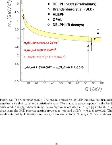
Figure 15: (left) Distributions of $\mathrm{B}_{3}$ determined using the Durham or JADE E0 jet finding algorithms before and after all corrections. The solid lines in the lower row of figures give the uncertainties on $\mathrm{B}_{3}$. The vertical dashed lines indicate the values of $y_{\mathrm{cut}}$ where the QCD predictions are calculated [221]. (right) Measurements of $m_{\mathrm{b}}(Q)$ at low and high energies $Q$ compared with the QCD expectation for the running of $m_{\mathrm{b}}(Q)$ [224].

Figure 15 (left) shows $\mathrm{B}_{3}(y_{\mathrm{cut}})$ measured by OPAL [221] before and after detector and hadronisation corrections for the JADE E0 and the Durham algorithm. One observes that the effect of the b quark mass is about 5% on $\mathrm{B}_{3}$ with reasonable uncertainties as indicated by the bands. The effect goes in opposite directions for JADE E0 and the Durham algorithm, because in the JADE type algorithms based on invariant mass to cluster jets the large b quark mass causes an enhancement of $\mathrm{B}_{3}$ while in the Durham algorithm the reduced phase space for hard gluon emission dominates thus reducing $\mathrm{B}_{3}$ [222].

Table 7: Values of $m_{\mathrm{b}}(m_{\mathrm{Z^{0}}})$ in units of GeV from various experiments with symmetrised systematic uncertainties. The last row shows the average determined as described in the text.

• Experiment	$m_{\mathrm{b}}(m_{\mathrm{Z^{0}}})$$\pm$	stat. $\pm$	syst. $\pm$	had. $\pm$	theo.
  ALEPH [223]	3.27$\pm$	0.22 $\pm$	0.22 $\pm$	0.38 $\pm$	0.16
  DELPHI [224]	2.96$\pm$	0.18 $\pm$	0.14 $\pm$	0.19 $\pm$	0.12
  OPAL [221]	2.67$\pm$	0.03 $\pm$	0.22 $\pm$	0.25 $\pm$	0.19
  SLD [222]	2.56$\pm$	0.27 $\pm$	0.33 $\pm$	0.84 $\pm$	0.44
  average	2.90$\pm$	0.12 $\pm$	0.29 $\pm$	0.20 $\pm$	0.14

Figure 15 (right) gives an overview over presently available measurements of $m_{\mathrm{b}}(m_{\mathrm{Z^{0}}})$ [224]. These are compared with low energy measurements and the QCD prediction for the running of $m_{\mathrm{b}}(Q)$. The predicted range of $m_{\mathrm{b}}(m_{\mathrm{Z^{0}}})$ is in good agreement with the measurements. The measurements of $m_{\mathrm{b}}(m_{\mathrm{Z^{0}}})$ of [221, 222, 223, 224] are averaged using the same method as for averaging values of $\alpha_{\mathrm{S}}$ (see section 4.4.1). The individual results are shown with symmetrised systematic uncertainties in table 7. The systematic uncertainty of the OPAL result was split into an experimental and a hadronisation uncertainty according to the average ratio of these uncertainties obtained from the individual jet algorithms. We assume the statistical errors to be uncorrelated and the experimental and hadronisation uncertainties to be partially correlated. The theory uncertainties are evaluated by simultaneous variation of the input values within their theory uncertainties. The average is shown in the last column of table 7. Combining all errors we find $m_{\mathrm{b}}(m_{\mathrm{Z^{0}}})=(2.90\pm 0.31)$ GeV, which may be compared with the average of low energy measurements $m_{\mathrm{b}}(m_{\mathrm{b}})=(4.24\pm 0.11)$ GeV [225]. The difference becomes $m_{\mathrm{b}}(m_{\mathrm{Z^{0}}})-m_{\mathrm{b}}(m_{\mathrm{b}})=(1.34\pm 0.33)$ GeV which is non-zero by four standard deviations thus providing strong experimental evidence for the running heavy quark mass in QCD.

5 Particle production

The direct observation of hadron production in $\mathrm{e^{+}e^{-}}$ annihilation offers unique ways to test predictions of QCD. The subject of multiplicities of hadrons is covered in detail in [226].

5.1 Low energy particles

Figure 16 (left) shows the production rates for inclusive and for identified charged hadrons ($\pi^{\pm}$, $K^{\pm}$, p) or hadrons decaying to final states with charged particles ($K^{0}$, $\phi$, $\Lambda$) as a function the particles scaled momentum fraction $x=2p/\sqrt{s}$ where $p$ is the particle momentum [227]. The momentum spectra of the various particles are fairly similar but their production rates are strongly suppressed with particle mass. The production rates for many particle species are summarised in [18].

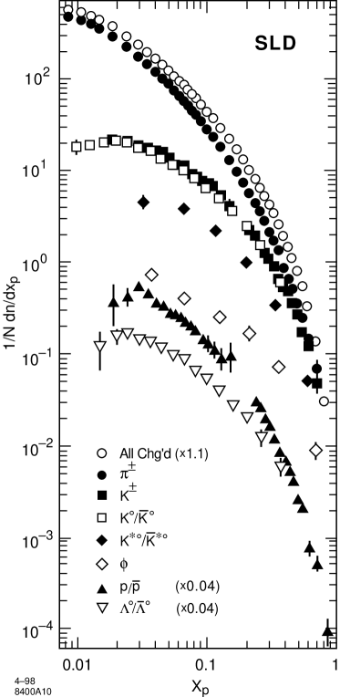
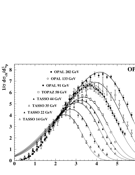
Figure 16: (left) Spectra of scaled momentum $x$ for identified particles as indicated and for all charged particles measured by SLD on the $\mathrm{Z^{0}}$ peak [227]. (right) Spectra of $\xi=\log(1/x)$ measured by OPAL using LEP 1 and LEP 2 data as well as lower energy data from TASSO [228]. The curves show fits of a NLLA QCD prediction [229] to the data.

The study of the observable $\xi=\ln(1/x)$, where $x$ is the scaled momentum or energy fraction defined above, allows to focus on the production mechanisms of low-momentum particles corresponding to large values of $\xi$. Figure 16 (right) shows the $\xi$ distributions measured by OPAL using all LEP 1 and LEP 2 data together with data from previous experiments [228]. A similar analysis is shown in [230]. Figure 17 (left) presents recent measurements by BES of $\xi$ at $\sqrt{s}=2.2$ to 4.8 GeV [231].

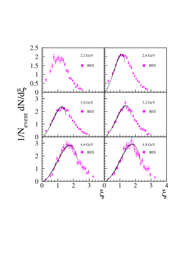
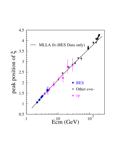
Figure 17: (left) Measurements of $\xi=\log(1/x)$ spectra at $2.2\leq\sqrt{s}\leq 4.8$ GeV by BES [231]. (right) Measurements of the peak position of $\xi$ distributions [231].

On both figures the typical hump-backed plateau [232] of the distributions is clearly visible. The distribution vanishes for small values of $\xi$ corresponding to large $x$ for kinematic reasons while the fall for large $\xi$ (small $x$) is due to destructive interference of coherent gluon radiation. Essentially, low energy gluons cannot resolve individual coloured partons anymore and are thus suppressed since an $\mathrm{e^{+}e^{-}}$ annihilation event is colourless. This explanation in the framework of perturbative QCD rests on the assumption that hadronisation is on average a local process. This assumption is referred to as local parton hadron duality (LPHD) [64, 232]. Assuming LPHD predicted spectra calculated for partons may be directly compared with measured spectra derived from the observed hadrons where only the relative normalisation is determined by experiment. The calculation in the modified leading-log approximation (MLLA) [233, 234, 235] is shown as solid lines in figure 17 (left) while the related NLLA QCD prediction [229] is shown as lines in figure 16 (right).

The position of the peaks $\xi^{*}$ of the $\xi$ distributions is seen to depend on the cms energy. This effect is predicted by MLLA QCD [235] and shown as the line on figure 17 (right). The fit was performed using only the low energy BES data and the result agrees well with the data up to LEP 1 energies.

Measurements of $\xi$ and $\xi^{*}$ have also been made for identified hadrons ($\pi^{\pm}$, K^±,0, p, $\Lambda$) as well as for identified quark flavours [130] and dependence on hadron mass and quark flavour has been observed. Distributions of $\xi$ at different $\sqrt{s}$ may be related directly via perturbative evolution equations in the MLLA [236].

5.2 High momentum particles and scaling violation

The fragmentation of partons produced in the hard interaction $\mathrm{e^{+}e^{-}}\rightarrow\mathrm{q\mathrm{\overline{q}}}(g)$ into hadrons is investigated using the scaled momentum of hadrons $x$. In the quark parton model, i.e. without strong interactions, one expects the distributions of $x$ measured at different cms energies to be identical. This prediction of a scaling behaviour is similar to the situation in deep inelastic scattering (DIS) of leptons on hadrons where $x_{Bj}=Q^{2}/(2m(E-E^{\prime}))$ with transferred 4-momentum $Q$, parton mass $m$, and lepton energies $E$ and $E^{\prime}$ before and after the scattering. Distributions of $x_{Bj}$ are independent of $Q^{2}$ in the quark parton model.

The scaling behaviour is modified or broken by strong interaction processes [237]. The probability for radiation of gluons from quarks depends on the energy scale of the quark and therefore due to the running of $\alpha_{\mathrm{S}}$ fewer hard gluons are produced at high energy. The scaled momentum $x$ spectra are expected to be softer at high energies. This is formally described by the theory with the Dokshitzer-Gribov-Lipatov-Altarelli-Parisi (DGLAP) evolution equations, see [238] and references therein. The normalised distribution of $x$ is described as the differential cross section $\sigma^{h}$ for production of a hadron with scaled momentum $x$:

$$\frac{1}{\sigma_{\mathrm{h}}}\frac{\mathrm{d}\sigma^{h}}{\mathrm{d}x}=\int_{x}^{1}\sum_{f\in\{udscbg\}}C_{f}(z,\alpha_{\mathrm{S}}(\mu_{\mathrm{R}}),x_{\mu})D_{f}(\frac{x}{z},\mu_{\mathrm{R}})\frac{\mathrm{d}z}{z}\;\;.$$ (41)

The coefficient functions $C_{f}(x,\alpha_{\mathrm{S}}(\mu_{\mathrm{R}}),x_{\mu})$ correspond to the probability to obtain a parton $f$ with scaled momentum $x$, where $f$ is either one of the five active quark flavours u, d, s, c, or b or a gluon g. The parameter $x_{\mu}=\mu_{\mathrm{R}}/Q$, with $Q=\sqrt{s}$, gives the renormalisation scale $\mu_{\mathrm{R}}$ where the coefficient and fragmentation functions are evaluated.

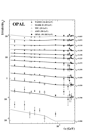
Figure 18: (left) Ratio of the inclusive charged particle $x$ spectra $1/sigmah\mathrm{d}\sigma^{h}/\mathrm{d}x$ measured by ALEPH at $\sqrt{s}\simeq 91$ GeV to data from TASSO measured at $\sqrt{s}=22$ GeV [239]. The lines present the result of a fit of the NLO QCD prediction (see text); the dashed shows the prediction with constant quark flavour composition. (right) Measurements of the normalised cross section for charged particle production in bins of $x$ as a function of $\sqrt{s}$ [228]. The solid lines show the result of a fit of the NLO QCD prediction (see text) while the dashed show an extrapolation of the fit result.

The fragmentation functions $D_{f}(x,\mu)$ correspond to the probability to obtain a hadron with momentum fraction $x$ from a parton $f$ at the momentum scale of the hard interaction $\mu$. The coefficient functions are known in NLO [240, 241]. The fragmentation functions are non-perturbative and thus cannot be calculated; they are the $\mathrm{e^{+}e^{-}}$ analog of parton density functions in DIS. However, the rate of change (evolution) of the $D_{f}(x,\mu)$ with changing hard scale $\mu$ is predicted by the DGLAP equations:

$$\frac{\mathrm{d}D_{f}(x,\mu)}{\mathrm{d}\ln\mu^{2}}=\sum_{i\in\{udscbg\}}\int_{x}^{1}P_{if}(z,\alpha_{\mathrm{S}}(\mu_{\mathrm{R}}),x_{\mu})D_{i}(\frac{x}{z},\mu)\frac{\mathrm{d}z}{z}$$ (42)

where the splitting functions $P_{ij}$ are also known in NLO QCD, see [238] and references therein. With these predictions one measurement at a reference scale $Q_{0}$ may be used to predict the $x$ distribution at another scale $Q$ with the strong coupling constant $\alpha_{\mathrm{S}}$ as a free parameter.

Figure 18 (left) shows the ratio of $x$ distributions measured by ALEPH at $\sqrt{s}=m_{\mathrm{Z^{0}}}$ and by TASSO at $\sqrt{s}=22$ GeV [239]. The smaller (larger) fraction of hadrons at large (small) $x$ at LEP 1 energies compared to $\sqrt{s}=22$ GeV is clearly visible. The solid line indicates the result of a fit of the NLO QCD prediction for this observable to several measurements of $x$ distributions at different energy scales. Figure 18 (right) presents the measurements by OPAL using LEP 1 and LEP 2 data together with measurements by previous experiments [228]. The solid lines show the QCD fit as explained above with $\alpha_{\mathrm{S}}=0.1182$ fixed and variable parametrisations of the fragmentation functions. The description of the data by the fit is adequate within the uncertainties. The result of a fit with $\alpha_{\mathrm{S}}(m_{\mathrm{Z^{0}}})$ as an additional free parameter is shown in table 8.

Table 8: Values of $\alpha_{\mathrm{S}}(m_{\mathrm{Z^{0}}})$ determined from analyses of scaling violation of $x$ spectra in $\mathrm{e^{+}e^{-}}$ annihilation. Experimental errors also include statistical uncertainties and uncertainties from parametrisation of non-perturbative fragmentation functions. The calculation of the average value is explained in the text.

• Experiment	$\alpha_{\mathrm{S}}(m_{\mathrm{Z^{0}}})$ $\pm$	expt. $\pm$	theo.
  ALEPH [239]	0.126 $\pm$	0.007 $\pm$	0.006
  DELPHI [242]	0.124 $\pm$	0.007 $\pm$	0.009
  OPAL [228]	0.113 $\pm$	0.005 $\pm$	0.007
  average	0.1192 $\pm$	0.0056 $\pm$	0.0070

Table 8 collects results for $\alpha_{\mathrm{S}}(m_{\mathrm{Z^{0}}})$ from analysis of scaling violation in $x$ spectra from $\mathrm{e^{+}e^{-}}$ annihilation to hadrons. All analyses are based on the same NLO QCD calculations for the coefficient and splitting functions and thus the results may be compared directly. We observe good agreement between the three values of $\alpha_{\mathrm{S}}(m_{\mathrm{Z^{0}}})$ within the experimental uncertainties. The average value of $\alpha_{\mathrm{S}}(m_{\mathrm{Z^{0}}})$ from analyses of scaling violation in $\mathrm{e^{+}e^{-}}$ annihilation is derived assuming the experimental uncertainties to be partially correlated while the theoretical uncertainties are accounted for by varying the input values simultanously within their theoretical errors. The result is shown in the last row of table 8 and is in good agreement with other determinations of $\alpha_{\mathrm{S}}(m_{\mathrm{Z^{0}}})$ discussed in this report. The weights of the individual results in the average are 0.35 (ALEPH), 0.15 (DELPHI) and 0.50 (OPAL). This determination of $\alpha_{\mathrm{S}}(m_{\mathrm{Z^{0}}})$ does not have explicit hadronisation uncertainties, because the inclusive measurement of hadron production results in a supression of non-perturbative effects with $1/Q^{2}$ [243]. Remaining hadronisation uncertainties enter as uncertainties of the parametrisation of the fragmentation functions $D_{f}$ and are thus part of the experimental errors.

Measurements of $x$ distributions for identified hadrons [227] have also been studied in global QCD analyses using perturbative evolution [244, 245] and good agreement between data and theory was found. The scaling violations of identified light and heavy (b) quark and gluon jets using LEP 1 and LEP 2 data has been measured and compared to NLO QCD predictions in [246]. The QCD predictions for $x$ spectra have been observed to be generally in good agreement with the data.

5.3 Longitudinal and transverse cross section

The measurement of the polar angle dependence of hadron production provides insight into the spin structure of the process $\mathrm{e^{+}e^{-}}\rightarrow\mathrm{hadrons}$ [238]. The normalised double differential cross section for hadron production in the process $\mathrm{e^{+}e^{-}}\rightarrow h+X$ is written as

$$\frac{1}{\sigma_{\mathrm{tot}}}\frac{\mathrm{d}^{2}\sigma^{h}}{\mathrm{d}x\mathrm{d}\cos\theta}=F_{T}(x)\frac{3}{8}(1+\cos^{2}\theta)+F_{L}(x)\frac{3}{4}\sin^{2}\theta+F_{A}(x)\frac{3}{4}\cos\theta$$ (43)

where $\sigma^{h}$ is the cross section for producing a hadron $h$, $x$ is the scaled momentum fraction of the hadron and $\theta$ is the angle between the hadron and electron beam directions. The fragmentation functions (FFs) are given by $F_{P}(x)=1/\sigma_{\mathrm{tot}}\mathrm{d}\sigma^{h}_{P}/\mathrm{d}x$, $P=T,L,A$. The first two terms stem from the polarisation states (transverse or longitudinal) of the intermediate vector boson ($\gamma$ or $\mathrm{Z^{0}}$) while the third term comes from parity violation of the electroweak interaction.

After integrating out the $\theta$ dependence only the $F_{T}(x)$ and $F_{L}(x)$ terms remain. As a result of energy conservation the integral

$$\frac{1}{2}\int_{0}^{1}x\frac{1}{\sigma_{\mathrm{tot}}}\frac{\mathrm{d}\sigma^{h}}{\mathrm{d}x}dx=\frac{1}{2}\mbox{$\langle x\rangle$}\mbox{$\langle n\rangle$}=1=\frac{\sigma_{\mathrm{T}}}{\sigma_{\mathrm{tot}}}+\frac{\sigma_{\mathrm{L}}}{\sigma_{\mathrm{tot}}}$$ (44)

where $\langle n\rangle$ is the average hadron multiplicity and $1/2\int xF_{P}(x)dx=\sigma_{P}$, $P=T,L$. The transverse and longitudinal cross sections $\sigma_{\mathrm{T}}$ and $\sigma_{\mathrm{L}}$ fulfil $\sigma_{\mathrm{T}}+\sigma_{\mathrm{L}}=\sigma_{\mathrm{tot}}$.

Measurements of the FFs $F_{P}(x)$, $P=T,L,A$ for charged hadrons have been performed by ALEPH, DELPHI and OPAL using large samples of hadronic $\mathrm{Z^{0}}$ decays [247, 239, 248]. The associated cross section ratios $\sigma_{\mathrm{T}}/\sigma_{\mathrm{tot}}$ and $\sigma_{\mathrm{L}}/\sigma_{\mathrm{tot}}$ for all hadrons are derived from the $F_{P}$ for charged hadrons assuming that the ratio of charged to neutral hadrons is identical for $\sigma_{\mathrm{T}}$ and $\sigma_{\mathrm{L}}$. This assumption is supported by studies of simulated events [247, 248]. A re-analysis of JADE data gave results for $\sigma_{\mathrm{T}}$ and $\sigma_{\mathrm{L}}$ at $\sqrt{s}=36.6$ GeV [249].

Figure 19 (left) shows the FFs determined by DELPHI and OPAL [248]. The analyses agree well with each other and a Monte Carlo model prediction (JETSET) is also found to agree with the data. The longitudinal FF $F_{L}$ is suppressed w.r.t. to the transverse FF $F_{T}$ reflecting the preferred polarisation of the intermediate gauge bosons. The presence of $F_{L}$ is understood as due to the possible presence of gluons in the final state. The results for $\sigma_{\mathrm{L}}$ are shown in figure 19 (right) [249] and compared with the JETSET Monte Carlo model prediction for partons and hadrons. The difference between the two lines for partons and hadrons indicates the presence of non-perturbative corrections. These power corrections have been calculated [250, 243] and were found to agree with the data [249].

Figure 19: (left) Fragmentation functions $F_{T}$ and $F_{L}$ measured by DELPHI and OPAL [248]. The lines show the prediction of the JETSET Monte Carlo model. (right) Measurements of $\sigma_{\mathrm{L}}/\sigma_{\mathrm{tot}}$ by DELPHI, OPAL and JADE compared with parton- and hadron-level predictions by the JETSET Monte Carlo model and a NLO QCD prediction [249] (see text for details).

The extraction of $\alpha_{\mathrm{S}}(m_{\mathrm{Z^{0}}})$ from the data can be done using the NLO prediction for the observable $\sigma_{\mathrm{L}}/\sigma_{\mathrm{tot}}$ [240, 248]. In order to obtain the best possible measurement we average the results for $\sigma_{\mathrm{L}}/\sigma_{\mathrm{tot}}$ from ALEPH, DELPHI and OPAL. The ALEPH measurements of $F_{L}(x)$ and $F_{T}(x)$ [239] are used to extract a value for $\sigma_{\mathrm{L}}/\sigma_{\mathrm{tot}}$ after estimating the missing contributions at $0<x<0.008$ using the ALEPH measurement of $\mbox{$\langle n_{\mathrm{ch.}}\rangle$}=21.91\pm 0.22$ [251] and the DELPHI measurement of $F_{L}(x)/(F_{L}(x)+F_{T}(x))=0.286\pm 0.021$ for $0<x<0.01$ [248]. The estimate uses the relation $\int_{0}^{1}F_{L}(x)+F_{T}(x)dx=\mbox{$\langle n_{\mathrm{ch.}}\rangle$}$. The result is $(\sigma_{\mathrm{L}}/\sigma_{\mathrm{tot}})_{\mathrm{ALEPH}}=0.0561\pm 0.0003\mathrm{(stat.)}\pm 0.0023\mathrm{(syst.)}$. The average of the ALEPH, DELPHI and OPAL results is computed assuming the experimental uncertainties to be uncorrelated with the result $\sigma_{\mathrm{L}}/\sigma_{\mathrm{tot}}=0.0558\pm 0.0021$. The value of $\alpha_{\mathrm{S}}(m_{\mathrm{Z^{0}}})$ is extracted based on the NLO QCD prediction [240, 248] combined with a hadronisation correction using JETSET derived from [247]. We find

$$\alpha_{\mathrm{S}}(m_{\mathrm{Z^{0}}})=0.1169\pm 0.0035\mathrm{(exp.)}\pm 0.0018\mathrm{(had.)}\pm 0.0072\mathrm{(theo.)}\;\;.$$ (45)

The hadronisation uncertainty is given by the difference of values for $\alpha_{\mathrm{S}}(m_{\mathrm{Z^{0}}})$ when HERWIG instead of JETSET is used to derive the hadronisation correction [247]. The theoretical uncertainty is evaluated by varying the renormalisation scale parameter in the range $0.5<x_{\mu}<2.0$ according to equation (6) and is consistent with [248].

The connection of the asymmetric FF $F_{A}(x)$ with parity violation in the electroweak interaction involving quarks has been investigated in [252]. A precise measurement of $F_{A}(x)$ could be converted into a measurement of the electroweak mixing angle $\sin\theta_{W}$ assuming that hadrons at high $x$ are likely to carry a quark produced in the $\mathrm{e^{+}e^{-}}$ annihilation. This prediction has been found to agree with data in [247, 248] but the precision of the measurements was insufficient to extract a value for $\sin\theta_{W}$.

5.4 Fragmentation of b quarks

The fragmentation process with heavy quarks is of special interest, because the large mass of the heavy quark provides a natural cutoff in perturbative QCD calculations (see e.g. [253, 254]). As a consequence reliable predictions of the perturbative part of the fragmentation process become possible. Assuming the b quark fragmentation process to be universal, precise measurements of the fragmentation of b quarks into b-flavoured hadrons with $\mathrm{e^{+}e^{-}}$ annihilation data can have consequences for the interpretation of hadron collider data for B meson production [255].

Figure 20 (left) presents as a representative example the measurement by SLD of the $x$ spectrum of B hadrons produced in $\mathrm{e^{+}e^{-}}$ annihilation at $\sqrt{s}\simeq m_{\mathrm{Z^{0}}}$ [256]. The variable $x=x_{B}=2E_{B}/\sqrt{s}$ corresponds to the scaled momentum variable discussed above, but due to the large B hadron masses the B hadron energy $E_{B}$ is used. Other recent measurements are [257, 258].

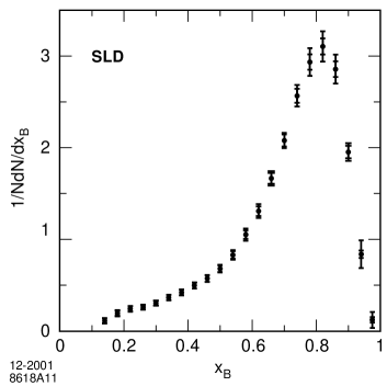
Figure 20: (left) Normalised $x$ spectrum of B hadrons produced in $\mathrm{e^{+}e^{-}}$ annihilation on the $\mathrm{Z^{0}}$ peak [256]. (right) Difference of charged particle multiplicity between light and b quark events $\delta_{\mathrm{bl}}$ measured by OPAL and other experiments at various cms energies [258]. The data are compared with several predictions as explained in the text.

The measurement of the $x$ spectrum of B hadrons is model dependent, because correcting the measured B hadron energies for experimental effects uses Monte Carlo simulations with models for the b quark fragmentation. The first step in Monte Carlo simulations is the parton shower which corresponds to a description of the perturbative part of the transition of a heavy quark into a observable heavy hadron. After the parton shower has stopped hadronisation models such as the Lund string model describe the formation of hadrons from the remaining quarks and gluons of the parton shower. The heavy quark fragmentation models specify how the energy of the heavy quark is transferred to a heavy hadron within the hadronisation process.

All recent measurements studied the consistency of various models for b quark fragmentation to B hadrons [257, 258, 256]. The best description of the observed $x$ spectra of B hadrons is obtained with the Bowler and with the Lund symmetric models implemented within the JETSET Monte Carlo event generator [258, 256, 259] (see the references for details on the fragmentation models). In particular the commonly used Peterson heavy quark fragmentation model is found to be disfavoured by the data.

This result is confirmed in a theoretical study [260] which unfolds the perturbative and the non-perturbative part of the description of the $x$ spectrum of B hadrons using the Mellin transform technique. Essentially, moments of the distribution are calculated and the unfolding is performed in moment space where it simplifies to a simple multiplication. The perturbative component is taken from JETSET or from a NLL perturbative QCD calculation. In both cases the Lund and the Bowler fragmentation functions are found to agree reasonably well with the extracted non-perturbative component while other fragmentation functions are disfavoured.

The radiation of soft gluons from heavy quarks with mass $m$ and energy $E$ is predicted to be suppressed within a cone around the heavy quark flight direction of opening angle $\alpha=m/E$ if $E>>M>>\Lambda_{\mathrm{QCD}}$. Assuming direct correspondence of parton and hadron distributions (LPHD as discussed above) allows to make predictions in MLLA QCD e.g. for the difference in charged particle multiplicities of light and heavy quark events, $\delta_{\mathrm{bl}}$ [45, 235, 261]. The MLLA QCD prediction is independent of cms energy and its latest value is $\delta_{\mathrm{bl}}=4.4\pm 0.4$ [261]. In contrast, the so-called naive prediction for $\delta_{\mathrm{bl}}$ considers only the reduction in phase space due to the heavy quark mass. Thus the observable $\delta_{\mathrm{bl}}$ becomes energy dependent and decreases with $\sqrt{s}$.

Figure 20 (right) shows a summary of measurements of $\delta_{\mathrm{bl}}$ at various cms energies [262]. The bands indicate the predictions from perturbative QCD and the naive model. The predictions become significantly different at high energies. The recent measurements using LEP 2 data by DELPHI [263] and OPAL allow to discriminate between the predictions and the naive model is clearly disfavoured by the data. The dash-dotted line presents an average of all measurements assuming energy independence: $\delta_{\mathrm{bl}}=3.05\pm 0.19$ which is significantly lower than the MLLA QCD prediction. This apparent discrepancy is of the order of important corrections beyond the MLLA [261].

5.5 Gluon splitting into heavy quarks

The gluon may split into a quark-antiquark pair; the process $\mathrm{g}\rightarrow\mathrm{q\mathrm{\overline{q}}}$ is one of the fundamental processes of QCD. When the virtual mass of the gluon is sufficiently large the splitting process can produce a pair of heavy (charm or bottom) quarks. In $\mathrm{e^{+}e^{-}}$ annihilation this process is rare, because it occurs only at $\mathcal{O}(\alpha_{\mathrm{S}}^{2})$. Neglecting quark masses one expects as a rough estimate at $\sqrt{s}=m_{\mathrm{Z^{0}}}$ a rate per hadronic $\mathrm{Z^{0}}$ decay $g_{\mathrm{q\mathrm{\overline{q}}}}\approx 1$ % where $q=b,c$.

The study of gluon splitting to heavy quarks is interesting for several reasons. The quark masses provide a natural infrared cutoff in a QCD calculation thus avoiding a usually present source of divergence and allowing for reliable predictions. The rates of gluon splitting into $\mathrm{b\overline{b}}$, $g_{\mathrm{b\overline{b}}}$, and into $\mathrm{c\overline{c}}$, $g_{\mathrm{c\overline{c}}}$, are an important source of uncertainty in the measurement of the partial widths for $\mathrm{Z^{0}}\rightarrow\mathrm{b\overline{b}}$ or $\mathrm{Z^{0}}\rightarrow\mathrm{c\overline{c}}$ decays. In particular the $\mathrm{Z^{0}}\rightarrow\mathrm{b\overline{b}}$ vertex is sensitive to possible effects of new physics coupling to the b-quark [264]. At high energy hadron colliders a large fraction of the observed B hadrons are thought to stem from gluon radiation via $\mathrm{g}\rightarrow\mathrm{b\overline{b}}$. Such processes are a major background to many searches for new particles decaying to heavy quarks like e.g. the Standard Model Higgs boson. In order to have precise predictions for the production rates of b-flavoured jets from QCD processes at hadron colliders the value of $g_{\mathrm{b\overline{b}}}$ must be known well. The most complete calculation [265] includes resummation of soft gluon contributions and predicts $g_{\mathrm{c\overline{c}}}=2.0$% and $g_{\mathrm{b\overline{b}}}=0.18$% for $\alpha_{\mathrm{S}}(m_{\mathrm{Z^{0}}})=0.118$, $m_{c}=1.2$ GeV and $m_{b}=5.0$ GeV.

For the measurement of $g_{\mathrm{c\overline{c}}}$ the ALEPH collaboration [266] classifies hadronic $\mathrm{Z^{0}}$ decays tagged by the presence of a $\mathrm{D}^{*}$ meson using the observable $\Delta M_{H}=M_{H}-M_{L}$, the difference between the scaled invariant masses of the heavy ($M_{H}$) and light ($M_{L}$) hemispheres of an event. It is expected that events containing the process $\mathrm{g}\rightarrow\mathrm{c\overline{c}}$ tend to have a larger $\Delta M_{H}$ due to the necessary presence of an energetic gluon jet. Figure 21 shows the $\Delta M_{H}$ spectrum of events where the $\mathrm{D}^{*}$ was found in the heavy hemisphere after subtraction of the measured contribution from primary charm production. There is clear evidence for the process $\mathrm{g}\rightarrow\mathrm{c\overline{c}}$ consistent with expectations. The other analyses from L3 [267] and OPAL [268] use the JADE jet clustering algorithm to find 3-jet events. The gluon jet is identified as the lowest energy jet or alternatively by OPAL also as the jet which splits into two at the largest value of $y_{\mathrm{cut}}$ using the JADE algorithm. Events with a charm tag in the gluon jet are counted as $\mathrm{g}\rightarrow\mathrm{c\overline{c}}$. The results are summarised in table 9.

Figure 21: Distribution of $\Delta M_{H}$ of events with a $\mathrm{D}^{*}$ in the heavy hemisphere after subtraction of the measured contribution from primary quarks [266]. The histogram shows the Monte Carlo prediction for the process $\mathrm{g}\rightarrow\mathrm{c\overline{c}}$.

The measurements of $g_{\mathrm{b\overline{b}}}$ of ALEPH [269], OPAL [270] and SLD [271] select 4-jet events in hadronic $\mathrm{Z^{0}}$ decays using the Durham algorithm; between about 10% to 15% of the events are selected. The jets are searched for the presence of displaced secondary vertices indicating B-hadron decays. Events with two such b-tags in two jets lying closely together in angle are considered as candidates originating from $\mathrm{g}\rightarrow\mathrm{b\overline{b}}$. The DELPHI analysis [272] measures the rate of $\mathrm{b\overline{b}}$$\mathrm{b\overline{b}}$ events in hadronic $\mathrm{Z^{0}}$ decays and the value of $g_{\mathrm{b\overline{b}}}$ is extracted using a theoretical calculation of $BR(\mathrm{Z^{0}}\rightarrow\mathrm{q\mathrm{\overline{q}}g},g\rightarrow\mathrm{b\overline{b}})/BR(\mathrm{Z^{0}}\rightarrow\mathrm{b\overline{b}}\mathrm{b\overline{b}})$. All results are shown in table 9.

Table 9: Results from various experiments for $g_{\mathrm{c\overline{c}}}$ and $g_{\mathrm{b\overline{b}}}$ with statistical errors and the uncorrelated and correlated systematic uncertainties as extracted from the references. The weights found in calculating the averages are also shown.

• 	$g_{\mathrm{c\overline{c}}}$	$\pm$stat.	$\pm$syst.	$\pm$syst.	weight
  	$\cdot 10^{-2}$		(uncorr.)	(corr.)
  ALEPH [266]	3.23	$\pm$0.48	$\pm$0.36	$\pm$0.39	0.12
  L3 [267]	2.45	$\pm$0.29	$\pm$0.32	$\pm$0.43	0.20
  OPAL [268]	3.20	$\pm$0.21	$\pm$0.18	$\pm$0.35	0.68
  average	3.05	$\pm$0.16	$\pm$0.14	$\pm$0.36
  	$g_{\mathrm{b\overline{b}}}$	$\pm$stat.	$\pm$syst.	$\pm$syst.	weight
  	$\cdot 10^{-3}$		(uncorr.)	(corr.)
  ALEPH [269]	2.77	$\pm$0.42	$\pm$0.28	$\pm$0.49	0.38
  DELPHI [272]	3.30	$\pm$1.00	$\pm$0.41	$\pm$0.67	0.06
  OPAL [270]	3.07	$\pm$0.53	$\pm$0.41	$\pm$0.88	0.09
  SLD [271]	2.44	$\pm$0.59	$\pm$0.13	$\pm$0.32	0.47
  average	2.67	$\pm$0.33	$\pm$0.13	$\pm$0.38

The averages are calculated based on uncorrelated and correlated systematic errors [273] extracted from the references given in table 9. The off-diagonal elements of the covariance matrix $V$ for the average are calculated from the correlated errors $\sigma_{i}$ and $\sigma_{j}$ of experiments $i$ and $j$ as $V_{ij,i\neq j}=\min(\sigma_{i},\sigma_{j})^{2}$. The resulting weights of the individual measurements in the averages are shown in the last column of table 9. The results shown here are consistent with those given in [274] but have slightly larger errors. The averages $g_{\mathrm{c\overline{c}}}=3.05\pm 0.42$% and $g_{\mathrm{b\overline{b}}}=0.267\pm 0.052$% are larger by two to three standard deviations than the theoretical predictions given above.

6 Inclusive observables

Inclusive observables are independent of the topology of the hadronic events. Prominent examples are $R_{\mathrm{e^{+}e^{-}}}=\sigma(\mathrm{e^{+}e^{-}}\rightarrow\mathrm{hadrons})/\sigma(\mathrm{e^{+}e^{-}}\rightarrow\mu^{+}\mu^{-})$, the analogous observable for Z-decays $R_{\mathrm{Z}}=\Gamma(\mathrm{Z^{0}}\rightarrow\mathrm{hadrons})/\Gamma(\mathrm{Z^{0}}\rightarrow\mathrm{leptons})$ or the hadronic branching ratio in $\tau$-decays $R_{\tau}=\Gamma(\tau\rightarrow\mathrm{hadrons})/\Gamma(\tau\rightarrow\mathrm{leptons})$. Inclusive observables depend on only one energy scale and are effectively QCD corrections to processes predicted by the electroweak theory involving quarks. The three observables $R_{\mathrm{e^{+}e^{-}}}$, $R_{\mathrm{Z}}$ and $R_{\tau}$ describe the QCD corrections to inclusive hadronic final states produced in decays of all electroweak gauge bosons $\gamma$, $\mathrm{Z^{0}}$ and $\mathrm{W^{\pm}}$. A comparison of the QCD corrections for these three different electroweak gauge boson decays to hadrons is an important consistency test of the theory of strong interactions.

Since QCD corrections to electroweak decays to hadrons generally scale in LO like $(1+\alpha_{\mathrm{S}}/\pi)$ at high energies careful measurements with uncertainties below ${\cal O}(1\%)$ are needed. The LEP experiments now provide precise measurements of electroweak observables such as cross sections from the line shape of the $\mathrm{Z^{0}}$ resonance or the decay widths of the $\mathrm{Z^{0}}$ boson. Another important set of results from LEP are precise measurements of hadronic and leptonic $\tau$ decays which form the basis for detailed studies of the large QCD corrections to the electroweak $\tau$ decay. Data for precision studies of $R_{\mathrm{e^{+}e^{-}}}$ come from the low energy experiments [275, 276].

6.1 $\mathrm{Z^{0}}$ properties

The LEP experiments have published their final results on electroweak observables and a consistent combination of the data is available [264]. The line shape of the $\mathrm{Z^{0}}$ resonance assuming lepton universality is described by the mass of the $\mathrm{Z^{0}}$ boson $m_{\mathrm{Z^{0}}}$, its total decay width $\Gamma_{\mathrm{Z}}$, the total hadronic cross section $\sigma_{\mathrm{h}}$, the ratio of hadronic and leptonic decay width of the $\mathrm{Z^{0}}$ boson $R_{\mathrm{Z}}$ and the leptonic pole forward-backward asymmetry $A_{\mathrm{FB}}^{\ell}$. In addition the partial decay widths to leptons, hadrons and invisible particles (neutrinos) $\Gamma_{\ell}$, $\Gamma_{\mathrm{h}}$ and $\Gamma_{\mathrm{inv}}$ are measured.

The results of the combination are preliminary but since the input values and the combination procedure [277] are final the results are not expected to change. The important QCD corrections to the electroweak observables derived from the $\mathrm{Z^{0}}$ resonance are known in NNLO QCD and rather precise determinations of the strong coupling $\alpha_{\mathrm{S}}(m_{\mathrm{Z^{0}}})$ become possible.

We concentrate here on a derived set of four electroweak observables with high sensitivity to QCD corrections [264]. These are $\Gamma_{\mathrm{h}}$, $R_{\mathrm{Z}}$ and the total cross sections for lepton and hadron production in $\mathrm{e^{+}e^{-}}$ annihilation $\sigma_{\ell}$ and $\sigma_{\mathrm{h}}$ on the peak of the $\mathrm{Z^{0}}$ resonance. These observables are related to $m_{\mathrm{Z^{0}}}$ and the partial and total decay widths:

$$R_{\mathrm{Z}}=\frac{\Gamma_{\mathrm{h}}}{\Gamma_{\ell}}\;,\;\;\sigma_{\mathrm{h}}=\frac{12\pi}{m_{\mathrm{Z^{0}}}^{2}}\cdot\frac{\Gamma_{\ell}\Gamma_{\mathrm{h}}}{\Gamma_{\mathrm{Z}}^{2}}\;\;\mathrm{and}\;\;\sigma_{\ell}=\frac{12\pi}{m_{\mathrm{Z^{0}}}^{2}}\cdot\frac{\Gamma_{\ell}^{2}}{\Gamma_{\mathrm{Z}}^{2}}\;\;.$$ (46)

Results for the partial decay widths are known with correlations [264] while correlations to $m_{\mathrm{Z^{0}}}$ are neglected. Using this information we derive the correlations between $\Gamma_{\mathrm{h}}$, $R_{\mathrm{Z}}$, $\sigma_{\mathrm{h}}$ and $\sigma_{\ell}$ as shown in table 10.

Table 10: Electroweak observables with high sensitivity to QCD corrections. The correlations were derived from correlations for the partial decay width of the $\mathrm{Z^{0}}$ assuming lepton universality [264].

• 			correlations
  Observable	Result		$\Gamma_{\mathrm{h}}$	$R_{\mathrm{Z}}$	$\sigma_{\mathrm{h}}$	$\sigma_{\ell}$
  $\Gamma_{\mathrm{h}}$[MeV]	1744.4 $\pm$	1.5	1.0
  $R_{\mathrm{Z}}$	20.767 $\pm$	0.025	0.62	1.0
  $\sigma_{\mathrm{h}}$[nb]	41.540 $\pm$	0.037	0.24	0.18	1.0
  $\sigma_{\ell}$[nb]	2.0003 $\pm$	0.0027	-0.40	-0.77	0.48	1.0

In order to extract values of $\alpha_{\mathrm{S}}(m_{\mathrm{Z^{0}}})$ from measurements of the electroweak observables we compare with the complete predictions including electroweak and QCD radiative corrections calculated with the electroweak library ZFITTER 6.41 [278]. The important QCD corrections are known to $\mathcal{O}(\alpha_{\mathrm{S}}^{3})$, e.g. for $\Gamma_{\mathrm{h}}$ [279, 280]. The value of $\alpha_{\mathrm{S}}(m_{\mathrm{Z^{0}}})$ is varied between 0.091 and 0.14 and the resulting predictions are interpolated until the experimental value is matched. The mass of the Higgs boson is taken to be $m_{\mathrm{H}}=114^{+69}_{-45}$ GeV [264]. Theoretical uncertainties are estimated by a consistent variation of the renormalisation scale [281] in the range $0.5<x_{\mu}<2$. In addition $m_{\mathrm{H}}$ is varied within its uncertainties. The four results for $\alpha_{\mathrm{S}}(m_{\mathrm{Z^{0}}})$ are shown in table 11 with experimental, theoretical and $m_{\mathrm{H}}$ uncertainties and their experimental correlations.

The theoretical uncertainties for $\Gamma_{\mathrm{h}}$ are consistent with an estimate based on the difference between the standard approach and an improved theoretical treatment which takes so-called $\pi^{2}$-terms into account [282]. An earlier estimate of the theoretical uncertainties when using $R_{\mathrm{Z}}$ is also consistent with our observed theoretical uncertainty [283].

A combined value of $\alpha_{\mathrm{S}}(m_{\mathrm{Z^{0}}})$ is derived from the individual values as a weighted average using the experimental covariance matrix with the theoretical and $m_{\mathrm{H}}$ errors added to the diagonal. The experimental error of the combined result is obtained from the experimental covariance matrix while the theoretical and $m_{\mathrm{H}}$ uncertainties are found by varying simultanously the renormalisation scale or $m_{\mathrm{H}}$ and repeating the combination. The combined result is shown in the last row of table 11. The individual values of $\alpha_{\mathrm{S}}(m_{\mathrm{Z^{0}}})$ are consistent within their experimental uncertainties with the average and the combination yields a value of $\chi^{2}/\mathrm{d.o.f.}=1.1$. The weights of the combination are 0.29 for $\Gamma_{\mathrm{h}}$, 0.25 for $R_{\mathrm{Z}}$, 0.17 for $\sigma_{\mathrm{h}}$ and 0.29 for $\sigma_{\ell}$. Changing the combination procedure to use only the experimental covariance matrix or including fully correlated theoretical and $m_{\mathrm{H}}$ uncertainties also in the off-diagonal elements of the covariance matrix yields deviations of the average smaller than 1%. The average value is in agreement with the final result for $\alpha_{\mathrm{S}}(m_{\mathrm{Z^{0}}})$ from jet and event shape observables discussed in section 4 and also with current world averages.

Table 11: Results for $\alpha_{\mathrm{S}}(m_{\mathrm{Z^{0}}})$ from electroweak observables with high sensitivity to QCD corrections. In each row the first error is experimental, the second is from variation of $x_{\mu}$ and the third is from variation of $m_{\mathrm{H}}$. The measurements are correlated as shown in table 10. The average value was obtained as described in the text.

• Observable	$\alpha_{\mathrm{S}}(m_{\mathrm{Z^{0}}})$ $\pm$	exp. $\pm$	scale $\pm$	$m_{\mathrm{H}}$
  $\Gamma_{\mathrm{h}}$	0.1221 $\pm$	0.0037 $\pm$	0.0020 $\pm$	0.0015
  $R_{\mathrm{Z}}$	0.1231 $\pm$	0.0037 $\pm$	0.0013 $\pm$	0.0005
  $\sigma_{\mathrm{h}}$	0.1075 $\pm$	0.0069 $\pm$	0.0006 $\pm$	0.0001
  $\sigma_{\ell}$	0.1187 $\pm$	0.0030 $\pm$	0.0011 $\pm$	0.0004
  average	0.1189 $\pm$	0.0027 $\pm$	0.0013 $\pm$	0.0007

This result may be viewed as one of the most reliable measurements of $\alpha_{\mathrm{S}}(m_{\mathrm{Z^{0}}})$, because the theoretical uncertainties are small due to the underlying NNLO QCD calculations and the inclusive nature of the observables. Uncertainties from measurements of the luminosity used to obtain cross sections are included in the experimental uncertainties. Uncertainties from non-perturbative contributions are expected to be negligible compared to the experimental errors as e.g. the leading power correction to the closely related observable $R_{\mathrm{e^{+}e^{-}}}$ was shown to scale like $1/Q^{6}$ where $Q=m_{\mathrm{Z^{0}}}$ is the hard scale of the process [78]. The uncertainty due to the unknown $m_{\mathrm{H}}$ may be as large as $\Delta\alpha_{\mathrm{S}}(m_{\mathrm{Z^{0}}})\simeq 0.003$ if ranges of $m_{\mathrm{H}}$ up to 1 TeV are considered [207]. However, such large Higgs boson masses would have consequences for the formulation of the electroweak theory and the whole procedure of extracting a precise value of $\alpha_{\mathrm{S}}(m_{\mathrm{Z^{0}}})$ would have to be reevaluated.

6.2 Decay of the $\tau$ lepton

Hadronic decays of the $\tau$ lepton offer unique possibilities to study the physics of strong interactions at low energy scales given by the mass of the $\tau$ lepton $m_{\tau}=1.777$ GeV. The interplay between perturbative and non-perturbative QCD effects is expected to play an important rôle. The ratio of decay widths of the $\tau$ lepton to hadronic and purely leptonic final states $R_{\tau}=\Gamma(\tau\rightarrow\mathrm{hadrons}\,\nu_{\tau})/\Gamma(\tau\rightarrow\ell\nu_{\ell})$ is an observable like $R_{\mathrm{e^{+}e^{-}}}$ and $R_{\mathrm{Z}}$. Leading electroweak effects cancel in the ratio and only QCD and rather small electroweak corrections remain.

A particularity of $\tau$ decays is the presence of a W boson in the weak decay instead of a $\mathrm{Z^{0}}$ or $\gamma$ in the case of $R_{\mathrm{Z}}$ or $R_{\mathrm{e^{+}e^{-}}}$. This leads to the possibility of hadronic final states with even or odd number of pions connected to vector (V) or axial-vector (A) currents which has interesting consequences for the size of non-perturbative contributions as discussed below. The contributions from perturbative and non-perturbative processes may be separated by studying the spectrum of invariant masses of the hadronic final states [284].

The LEP experiments ALEPH and OPAL have analysed hadronic final states from $\tau$ decays using large samples of $\mathrm{Z^{0}}$ decays produced on resonance [285, 286]. In the ALEPH (OPAL) analysis 124k (150k) $\tau$ pair candidate events are used. Figure 22 (upper row) shows the spectral functions $v(s)=\mathrm{d}R_{\tau,v}/\mathrm{d}s$ and $a(s)=\mathrm{d}R_{\tau,a}/\mathrm{d}s$ with $R_{\tau,v/a}(s)=\Gamma(\tau\rightarrow\mathrm{pions}\,\nu_{\tau})/\Gamma(\tau\rightarrow\rme\nu_{e}\nu_{\tau})$ of hadronic $\tau$ decays into final states with an even or odd number of pions. The variable $s$ denotes the invariant mass of the hadronic final state. In the figures the small corrections based on Monte Carlo simulation for unobserved final states are also indicated. In the lower row the sum and the difference of the vector and axial vector spectral functions $v(s)$ and $a(s)$ are shown.

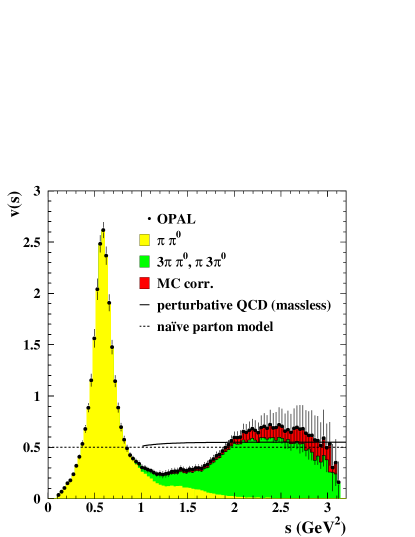
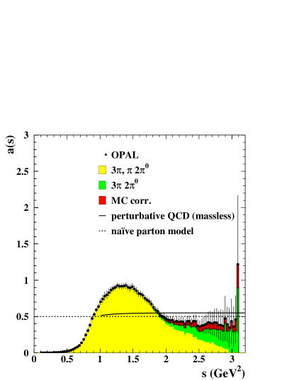
Figure 22: (upper row) Spectral functions for hadronic $\tau$ decays to final states with even (v(s)) or odd (a(s)) number of pions. The shaded areas show contributions from hadronic final states as indicated and the Monte Carlo (MC) based correction for unobserved final states. (lower row) Sum or difference of the spectral functions. The lines show predictions as indicated on the figures. All figures from [286].

The dashed and solid lines in figure 22 show the predictions by the naive parton model and perturbative QCD with massless partons and $\alpha_{\mathrm{S}}(m_{\mathrm{Z^{0}}})=0.122$. The pQCD predictions are seen to agree well with the inclusive $v(s)+a(s)$ spectral function while for $v(s)$ and $a(s)$ the prediction lies below or above the data. This observation already indicates that there are significant non-perturbative contributions to $v(s)$ and $a(s)$ which, however, largely cancel in the sum $v(s)+a(s)$.

For the detailed analysis moments of the spectral functions are determined [284]:

$$R_{\tau,v/a}^{kl}(s_{0})=\int_{0}^{s_{0}}\left(1-\frac{s}{s_{0}}\right)^{k}\left(\frac{s}{m_{\tau}^{2}}\right)^{l}\frac{\mathrm{d}R_{\tau,v/a}}{\mathrm{d}s}ds$$ (47)

for $kl=00,10,11,12,13$. These moments are constructed such that they are theoretically and experimentally well under control. The moment $R_{\tau,v/a}^{00}(s_{0}=m_{\tau}^{2})=R_{\tau}$ corresponds to the usual hadronic branching ratio in $\tau$ decays.

The theoretical prediction is formulated as a sum of perturbative and non-perturbative QCD contributions:

$$R_{\tau,v/a}^{kl}(s_{0})=\frac{3}{2}S_{EW}|V_{ud}|^{2}\left(1+\delta_{EW}^{kl}+\delta_{\mathrm{pert}}^{kl}+\delta_{\mathrm{non-pert},v/a}^{kl}\right)$$ (48)

where $S_{EW}=1.0194$, $V_{ud}=0.9745\pm 0.0004$ [18] and $\delta_{EW}^{00}=0.001$. The term $\delta_{pert}^{kl}$ contains the perturbative QCD part known to $\mathcal{O}(\alpha_{\mathrm{S}}^{3})$ [27, 287, 288]. The original calculation of [288] has been improved in [289] by a more accurate treatment of the running strong coupling in the calculation using the full $\beta$-function instead of an approximation. A third calculation includes a resummation of the effects of renormalon chains [290]. The non-perturbative contribution can be analysed in the framework of the Operator Product Expansion (OPE) as a power series in terms of $1/m_{\tau}^{2}$ [288]

$$\delta_{\mathrm{non-pert},v/a}^{kl}=\sum_{D=2,4,6,\ldots}\delta_{v/a}^{D,kl}\;\;\;.$$ (49)

The first term ($D=2$) in equation (49) is a correction for finite parton masses and can be calculated perturbatively. The $D=4,6,8$ terms are studied as non-perturbative corrections in the analyses.

As already indicated by figure 22 the non-perturbative corrections turn out to be consistent with zero when moments of the inclusive spectral function $v(s)+a(s)$ are analysed. The correction terms are found to be of roughly the same size but opposite sign when moments of $v(s)$ and $a(s)$ are studied individually [285, 286].

The analysis of the perturbative term $\delta_{pert}^{kl}$ allows a precise determination of the strong coupling constant at energy scales given by the mass of the $\tau$ lepton $m_{\tau}=1777.0\pm 0.3$ GeV [18] essentially free of non-perturbative uncertainties.

Following [285, 286] the determination of $\alpha_{\mathrm{S}}$ from hadronic $\tau$ decays using $R_{\tau}=R_{\tau}^{00}$ is updated for recent values of the $\tau$ lifetime $\tau_{\tau}=290.6\pm 1.1$ ps and the branching ratio $B_{\mu}=B(\tau\rightarrow\mu\nu_{\mu}\nu_{\tau})=0.1736\pm 0.0006$ [18]. The contribution of strange hadronic $\tau$ decays is subtracted using $R_{\tau,S}=0.1677\pm 0.005$ [291]. We find for the non-strange branching ratio $R_{\tau}=3.468\pm 0.011$. A similar study [292] using preliminary ALEPH data [293] finds $R_{\tau}=3.471\pm 0.011$ in agreement with our result. The improved calculation of [289] is chosen to extract a value for $\alpha_{\mathrm{S}}$. The ${\cal O}(\alpha_{\mathrm{S}}^{4})$ term is set to zero, because for consistency with other determinations of $\alpha_{\mathrm{S}}$ discussed in this report we prefer to extract a value of $\alpha_{\mathrm{S}}$ without the additional assumptions needed to estimate the ${\cal O}(\alpha_{\mathrm{S}}^{4})$ term [294] . We find

$$\alpha_{\mathrm{S}}(m_{\tau})=0.347\pm 0.005\mathrm{(exp.)}\pm 0.003\mathrm{(non-pert.)}\pm 0.018\mathrm{(theo.)}$$ (50)

The non-perturbative correction was set to $\delta_{\mathrm{non-pert},v+a}=-0.0024\pm 0.0025$ [286] (consistent with $\delta_{\mathrm{non-pert},v+a}=-0.0048\pm 0.0017$ [293]) and varied within its errors in order to obtain the uncertainty due to non-perturbative effects. The theoretical error was determined by a variation of the renormalisation scale in the range $0.5<x_{\mu}<2.0$. We take the larger variation from changing $x_{\mu}$ to define the theoretical uncertainty. We did not consider a variation of the renormalisation scheme as done in [286] in order to be consistent with other determinations of $\alpha_{\mathrm{S}}$ discussed in this report. After evolving to the $\mathrm{Z^{0}}$ mass scale using the 3-loop $\beta$-function and 2-loop matching at the crossing of heavy quark thresholds [20] we find

$$\alpha_{\mathrm{S}}(m_{\mathrm{Z^{0}}})=0.1221 \pm 0.0006\mathrm{(exp.)}\pm 0.0004\mathrm{(non-pert.)}$$

$$\pm 0.0019\mathrm{(theo.)}\pm 0.0003\mathrm{(evol.)}\;\;.$$

The last error $\mathrm{(evol.)}$ is due to uncertainties in the evolution procedure. The evolution of $\alpha_{\mathrm{S}}(m_{\tau})$ to $\alpha_{\mathrm{S}}(m_{\mathrm{Z^{0}}})$ takes the crossing of the charm and bottom quark threshold into account by setting the charm quark mass to $m_{c}=1.778$ GeV. The uncertainty due to the evolution procedure is evaluated following [295] by setting the matching thresholds to $m_{c}=4$ GeV or $m_{b}=20$ GeV and by changing the absolute quark masses within their uncertainties [18].

The analogous determination of $\alpha_{\mathrm{S}}(m_{\tau})$ and $\alpha_{\mathrm{S}}(m_{\mathrm{Z^{0}}})$ using the calculation of [290] results in $\alpha_{\mathrm{S}}(m_{\tau})=0.303\pm 0.003\mathrm{(exp.)}\pm 0.002\mathrm{(non-pert.)}\pm 0.011\mathrm{(theo.)}$ and $\alpha_{\mathrm{S}}(m_{\mathrm{Z^{0}}})=0.1166\pm 0.0004\mathrm{(exp.)}\pm 0.0003\mathrm{(non-pert.)}\pm 0.0015\mathrm{(theo.)}\pm 0.0003\mathrm{(evol.)}$. The difference between the result in equation (6.2) and this result is $\Delta\alpha_{\mathrm{S}}(m_{\mathrm{Z^{0}}})=0.0055$ which corresponds to less than three standard deviations of the total errors. However, since the calculation of [290] is rather different compared to e.g. [289] such discrepancies might be expected. In [214] the strong coupling constant is extracted using the ALEPH data [285] and a renormalisation group invariant formulation of the perturbative QCD prediction. Their result is $\alpha_{\mathrm{S}}(m_{\mathrm{Z^{0}}})=0.1184\pm 0.0007\mathrm{(exp.)}\pm 0.0019\mathrm{(theo.)}\pm 0.0006\mathrm{(evol.)}$ which is in fair agreement with (6.2). A similar result was found in [296]. The difference between using the calculation of [288] and the improved calculation of [289] is $\Delta\alpha_{\mathrm{S}}(m_{\mathrm{Z^{0}}})\simeq 0.003$ [286]. Using the prediction of [289] including the estimate of the ${\cal O}(\alpha_{\mathrm{S}}^{4})$ term as in [286] we find $\Delta\alpha_{\mathrm{S}}(m_{\mathrm{Z^{0}}})=-0.0006$.

This measurement of $\alpha_{\mathrm{S}}(m_{\mathrm{Z^{0}}})$ shown in equation (6.2) has comparable uncertainties to and is consistent with the measurement using the $\mathrm{Z^{0}}$ line shape observables discussed in section 6.1. Even though the difference between different methods of extracting $\alpha_{\mathrm{S}}(m_{\mathrm{Z^{0}}})$ from the hadronic $\tau$ data appears large it corresponds to about three times the total uncertainties. We conclude that the determination of $\alpha_{\mathrm{S}}(m_{\mathrm{Z^{0}}})$ from hadronic $\tau$ decays is reliable within the reasonably well estimated total errors.

6.3 $\mathrm{e^{+}e^{-}}$ annihilation at low energies

In the $\mathrm{e^{+}e^{-}}$ annihilation to hadrons at low energies the intermediate gauge boson is predominantly a photon thus giving access to the process $\gamma\rightarrow\mathrm{q\mathrm{\overline{q}}}$. The quantity of interest is $R_{\mathrm{e^{+}e^{-}}}=\sigma(\mathrm{e^{+}e^{-}}\rightarrow\mathrm{hadrons})/\sigma(\mathrm{e^{+}e^{-}}\rightarrow\mu^{+}\mu^{-})$, because many experimental and theoretical uncertainties introduced by selection efficiency corrections or radiative corrections are reduced in the ratio. Many measurements exist and have been summarised in other reviews, see e.g. [197, 297, 18]. Theoretical predictions for this observable exist in $\mathcal{O}(\alpha_{\mathrm{S}}^{3})$ [27, 36].

In [197] a consistent analysis of $R_{\mathrm{e^{+}e^{-}}}$ using TRISTAN and PETRA data [298] is used to extract the strong coupling constant in $\mathcal{O}(\alpha_{\mathrm{S}}^{3})$ with the result $\alpha_{\mathrm{S}}(42.4~{}\mathrm{GeV})=0.175\pm 0.028$ or $\alpha_{\mathrm{S}}(m_{\mathrm{Z^{0}}})=0.126\pm 0.022$. The measurements of $R_{\mathrm{e^{+}e^{-}}}$ take account of the $\mathrm{Z^{0}}$ mass measured at LEP and also include improved electroweak radiative corrections.

The CLEO collaboration has measured $R_{\mathrm{e^{+}e^{-}}}$ at $\sqrt{s}=10.52$ GeV, i.e. just below the Y(4S) resonance. A QCD prediction including heavy quark masses and corrected for QED radiation is used to extract $\alpha_{\mathrm{S}}(10.52~{}\mathrm{GeV})=0.20\pm 0.01\mathrm{(stat.)}\pm 0.06\mathrm{(syst.)}$. For the evolution to the $\mathrm{Z^{0}}$ mass scale we use a b quark threshold of 10.53 GeV such that the value $\alpha_{\mathrm{S}}(10.52~{}\mathrm{GeV})=0.20$ is interpreted as the strong coupling in a regime with four active quark flavours. The result is

$$\alpha_{\mathrm{S}}(m_{\mathrm{Z^{0}}})=0.130\pm 0.004\mathrm{(stat.)}\pm 0.025\mathrm{(syst.)}$$ (52)

in good agreement with previous results. The dependence of this result on the actual value of the b quark threshold and the b quark mass $m_{b}=4.25\pm 0.15$ GeV [18] in the $\overline{\mathrm{MS}}$ scheme is negligible.

The behaviour of $R_{\mathrm{e^{+}e^{-}}}(s)$ at low values of $s$ in the region of hadronic resonances may be described by perturbative QCD in the same way as the spectral functions from hadronic $\tau$ decays [275]. The perturbative prediction for $R_{\mathrm{e^{+}e^{-}}}$ is written in terms of a the so-called Adler D-function:

$$R_{\mathrm{e^{+}e^{-}}}(s_{0})=\frac{1}{2\pi i}\oint_{s=s_{o}}\frac{D(s)}{s}ds$$ (53)

where the D-function $D(s)$ is known in $\mathcal{O}(\alpha_{\mathrm{S}}^{3})$ [27, 36]. Non-perturbative effects are treated by applying the OPE to moments of $R_{\mathrm{e^{+}e^{-}}}(s)$:

$$R_{\mathrm{e^{+}e^{-}}}^{kl}(s_{0})=\int_{4m_{\pi}^{2}}^{s_{0}}\left(1-\frac{s}{s_{0}}\right)^{k}\left(\frac{s}{s_{0}}\right)^{l}\frac{R_{\mathrm{e^{+}e^{-}}}(s)}{s_{0}}ds\;\;\;.$$ (54)

Similar to the case of hadronic $\tau$ decays the complete prediction for $D(s)$ is a sum of perturbative and non-perturbative terms. The non-perturbative part of $D(s)$ in the OPE is a power series in terms of $1/s^{n}$ starting at $n=3$.

In [276] the same data as in [275] are used to determine the moments $R_{\mathrm{e^{+}e^{-}}}^{kl}(4~{}\mathrm{GeV}^{2}),kl=20,30,31,32,33$. A simultaneous fit of the QCD prediction for these moments with $\alpha_{\mathrm{S}}(2~{}\mathrm{GeV})$, the strange quark mass and the first two non-perturbative terms proportional to $1/s^{3}$ and $1/s^{4}$ gives a good description of the data. The result for the strong coupling constant is $\alpha_{\mathrm{S}}(2~{}\mathrm{GeV})=0.286\pm 0.031\mathrm{(exp.)}\pm 0.015\mathrm{(theo.)}$ corresponding to

$$\alpha_{\mathrm{S}}(m_{\mathrm{Z^{0}}})=0.117\pm 0.005\mathrm{(exp.)}\pm 0.002\mathrm{(theo.)}\;\;\;.$$ (55)

Compared to the result from hadronic $\tau$ decays shown in equation (6.2) the theoretical uncertainties are similar while the experimental errors are larger. Within the uncertainties the measurements from hadronic $\tau$ and $\mathrm{Z^{0}}$ decays and from hadron production in $\mathrm{e^{+}e^{-}}$ annihilation are consistent. New measurements of hadron production in $\mathrm{e^{+}e^{-}}$ annihilation at low $\sqrt{s}$ promise to allow reduced experimental uncertainties in the future [299] such that this measurement should have competitive uncertainties.

7 Summary of $\alpha_{\mathrm{S}}$ determinations

In this section we collect and systematically compare all significant measurements of the strong coupling constant $\alpha_{\mathrm{S}}(m_{\mathrm{Z^{0}}})$ discussed in this report. We concentrate on reliable measurements with comparatively small uncertainties in order to probe the consistency of the theory in the best possible way.

Table 12 presents the results selected from various sections of this report. The first two rows of the table contain the results based on $\mathcal{O}(\alpha_{\mathrm{S}}^{2})$+NLLA QCD with hadronisation correction performed using Monte Carlo simulation. As discussed in section 4.4.1 the analyses from JADE and LEP use the same set of 3-jet event shape observables sensitive to $\alpha_{\mathrm{S}}$ in $\mathcal{O}(\alpha_{\mathrm{S}})$. The ALEPH, DELPHI and OPAL analysis (see section 4.4.2) based on the 4-jet fraction $\mathrm{R}_{4}$ are sensitive to $\alpha_{\mathrm{S}}$ in $\mathcal{O}(\alpha_{\mathrm{S}}^{2})$. ALEPH and OPAL use NLO+NLLA calculations and the Durham algorithm while DELPHI uses NLO calculations with experimentally optimised renormalisation scale and the Cambridge algorithm.

A direct comparison of the results from JADE and LEP shows very good agreement. As the set of observables is identical and the analysis procedures are rather similar the good agreement shows that a consistent analysis of 3-jet event shape observables is possible from the lowest PETRA/JADE cms energies of 14 GeV to the highest LEP 2 cms energies of about 200 GeV. The results from analysis of $\mathrm{R}_{4}$ are consistent with the other NLO values within the uncertainties. This confirms that the calculation of radiative corrections within perturbative QCD is consistent within this set of rather different observables.

Table 12: Summary of determinations of $\alpha_{\mathrm{S}}(m_{\mathrm{Z^{0}}})$ based on observables, theoretical calculations and experiments as indicated. The experimental errors (exp.) also include statistical errors. Numbers covering two columns represent combined errors. The observables $\mathrm{R_{4}(D)}$ and $\mathrm{R_{4}(C)}$ refer to $\mathrm{R}_{4}$ using the Durham or Cambridge jet finding algorithm.

		Experiments
Observable	Theory	(Q [GeV])	$\alpha_{\mathrm{S}}(m_{\mathrm{Z^{0}}})$	$\pm$exp.	$\pm$had.	$\pm$theo.
3-jet shp.	NLO+NLLA	JADE (14-44)	0.1203	0.0018	0.0053	0.0050
3-jet shp.	NLO+NLLA	LEP (91-207)	0.1201	0.0009	0.0019	0.0049
$\mathrm{R_{4}(D)}$	NLO+NLLA	ALEPH (91)	0.1170	0.0009	0.0010	0.0017
$\mathrm{R_{4}(D)}$	NLO+NLLA	OPAL (91-207)	0.1182	0.0015	0.0011	0.0018
$\mathrm{R_{4}(C)}$	NLO	DELPHI (91)	0.1175	0.0011	0.0027	0.0007
sc. viol.	NLO	LEP (14-207)	0.1192	0.0056	0.0070
$\sigma_{\mathrm{L}}/\sigma_{\mathrm{tot}}$	NLO	LEP (91)	0.1169	0.0035	0.0018	0.0072
$\Gamma_{\mathrm{h}}$, $R_{\mathrm{Z}}$, $\sigma_{\mathrm{h}}$, $\sigma_{\ell}$	NNLO	LEP/SLD (91)	0.1189	0.0027	-	0.0015
$R_{\tau}$	NNLO	$\mathrm{e^{+}e^{-}}$ (1.777)	0.1221	0.0006	0.0004	0.0019
$R_{\mathrm{e^{+}e^{-}}}$	NNLO	$\mathrm{e^{+}e^{-}}$ (2)	0.117	0.005	0.002

Having observed good consistency between the 3-jet results we construct an average value of the results from JADE and LEP assuming that statistical errors are uncorrelated and experimental and hadronisation errors are partially correlated. Theoretical errors are treated as in the combinations of $\alpha_{\mathrm{S}}$ in section 4.4.1. The result for $\alpha_{\mathrm{S}}(m_{\mathrm{Z^{0}}})$ from 3-jet event shapes using NLO+NLLA QCD predictions is

$$\alpha_{\mathrm{S}}(m_{\mathrm{Z^{0}}})=0.1202 \pm 0.0004\mathrm{(stat.)}\pm 0.0009\mathrm{(exp.)}$$

$$\pm 0.0025\mathrm{(had.)}\pm 0.0049\mathrm{(theo.)}\;\;.$$

The weights are 0.32 for the JADE result and 0.68 for the LEP result. The determination of $\alpha_{\mathrm{S}}(m_{\mathrm{Z^{0}}})$ in $\mathcal{O}(\alpha_{\mathrm{S}}^{2})$+NLLA from 3-jet event shape observables has a fairly large theoretical uncertainty compared with some other measurements. This uncertainty might be reduced substantially when complete NNLO calculations for 3-jet production in $\mathrm{e^{+}e^{-}}$ annihilation will become available [25, 26].

The measurements of $\alpha_{\mathrm{S}}(m_{\mathrm{Z^{0}}})$ from $\mathrm{R}_{4}$ discussed in section 4.4.2 have small uncertainties. However, since no other comparable measurements based on different 4-jet observables exist consistency checks were not possible. For the purpose of presentation we combine the ALEPH and OPAL measurements based on $\mathrm{R_{4}(D)}$ using the Durham algorithm and NLO+NLLA theory and the DELPHI measurement based on $\mathrm{R_{4}(C)}$ using the Cambridge algorithm and NLO theory. Experimental errors are assumed as partially correlated while hadronisation and theoretical uncertainties are treated by simultaneous variation of the input values within their individual errors. The result from analyses of 4-jet fractions $\mathrm{R}_{4}$ becomes $\alpha_{\mathrm{S}}(m_{\mathrm{Z^{0}}})=0.1175\pm 0.0002\mathrm{(stat.)}\pm 0.0010\mathrm{(exp.)}\pm 0.0014\mathrm{(had.)}\pm 0.0015\mathrm{(theo.)}$.

The result from the NLO analyses of scaling violation (sc. viol.) in $\mathrm{e^{+}e^{-}}$ annihilation to hadrons is discussed in section 5.2. The method is inclusive and thus has negligible hadronisation uncertainties. There is good agreement with the results from other observables. However, since the QCD calculations are limited to NLO a direct comparison and combination with other inclusive measurements of $\alpha_{\mathrm{S}}(m_{\mathrm{Z^{0}}})$ based on NNLO QCD discussed below is not attempted.

The seventh row of table 12 gives the result of the NLO analysis of the ratio of longitudinal to total cross section $\sigma_{\mathrm{L}}/\sigma_{\mathrm{tot}}$ from section 5.3. Combining all available measurements of this observable and using the hadronisation corrections derived from [247] yields a consistent measurement of $\alpha_{\mathrm{S}}(m_{\mathrm{Z^{0}}})$ with a significantly reduced experimental error compared with [248]. This measurement is combined with the determination of $\alpha_{\mathrm{S}}(m_{\mathrm{Z^{0}}})$ from scaling violations assuming experimental errors as partially correlated while hadronisation and theory errors are treated by simultaneous variation of the input values within their hadronisation or theoretical uncertainties. We find for $\alpha_{\mathrm{S}}(m_{\mathrm{Z^{0}}})$ from analysis of fragmentation in $\mathrm{e^{+}e^{-}}$ annihilation to hadrons:

$$\alpha_{\mathrm{S}}(m_{\mathrm{Z^{0}}})=0.1179\pm 0.0040\mathrm{(exp.)}\pm 0.0010\mathrm{(had.)}\pm 0.0071\mathrm{(theo.)}\;\;.$$ (57)

The lower three rows of table 12 present results from the inclusive observables discussed in section 6 derived using $\mathcal{O}(\alpha_{\mathrm{S}}^{3})$ (NNLO) QCD calculations. The inclusive nature of the observables allows the calculation in $\mathcal{O}(\alpha_{\mathrm{S}}^{3})$ containing two-loop radiative corrections and reduces uncertainties from non-perturbative effects. The results for $\alpha_{\mathrm{S}}(m_{\mathrm{Z^{0}}})$ from the $\mathrm{Z^{0}}$ line shape observables $\Gamma_{\mathrm{h}}$, $R_{\mathrm{Z}}$, $\sigma_{\mathrm{h}}$ and $\sigma_{\ell}$ and from analysis of $R_{\tau}$ are in agreement within less than two standard deviations of their total uncertainties. The good agreement of the precise values of $\alpha_{\mathrm{S}}(m_{\mathrm{Z^{0}}})$ from the $\mathrm{Z^{0}}$ line shape observables and $R_{\tau}$ at the level of $\Delta\alpha_{\mathrm{S}}(m_{\mathrm{Z^{0}}})=0.0032\pm 0.0032$ may be viewed as a strong test of asymptotic freedom, since two measurements obtained at energy scales differing by a factor of ${\cal O}(100)$ are compared. In the calculation of the error of $\Delta\alpha_{\mathrm{S}}(m_{\mathrm{Z^{0}}})$ only the smaller of the theoretical uncertainties was considered.

We derive an average value of the NNLO results assuming statistical errors as uncorrelated and experimental errors to be partially correlated. Hadronisation and theoretical uncertainties are treated by simultaneous variation of the input values within their uncertainties. The result for $\alpha_{\mathrm{S}}(m_{\mathrm{Z^{0}}})$ from inclusive observables in NNLO QCD is

$$\alpha_{\mathrm{S}}(m_{\mathrm{Z^{0}}})=0.1211\pm 0.0010\mathrm{(exp.)}\pm 0.0018\mathrm{(theo.)}$$ (58)

where statistical errors have been included in the experimental error and hadronisation uncertainties are included in the theory error. The weights are 0.27 for the $\mathrm{Z^{0}}$ line shape observables, 0.70 for $R_{\tau}$ and 0.03 for $R_{\mathrm{e^{+}e^{-}}}$ with $\chi^{2}/\mathrm{d.o.f.}=1.05/2$. The consistency between the three results is impressive as indicated by the $\chi^{2}/\mathrm{d.o.f.}$ value. This result is considered to be the most reliable determination of the strong coupling constant $\alpha_{\mathrm{S}}(m_{\mathrm{Z^{0}}})$ discussed in this report, because it is based on NNLO QCD calculations and has only small uncertainties from modelling of non-perturbative effects. Further improvements of this determination of $\alpha_{\mathrm{S}}(m_{\mathrm{Z^{0}}})$ may be expected from new measurements of $R_{\mathrm{e^{+}e^{-}}}$ in the low energy region leading to a reduction of the experimental uncertainties [299].

Figure 23 summarises the high precision measurements of $\alpha_{\mathrm{S}}$ discussed in this section. The data are compared with our average of NNLO QCD based determinations of $\alpha_{\mathrm{S}}(m_{\mathrm{Z^{0}}})$ given in equation (58) shown as lines and grey band. The value of $\alpha_{\mathrm{S}}(m_{\mathrm{Z^{0}}})$ is evolved in NNLO to other cms energies $\sqrt{s}$ as explained in section 2.1. The consistency between the predicted behaviour of $\alpha_{\mathrm{S}}(\sqrt{s})$ using only the NNLO observables with the other measurements is good; this shows that QCD successfully describes many important features of hadron production in $\mathrm{e^{+}e^{-}}$ annihilation at scales covering two orders of magnitude from $m_{\tau}$ to the highest LEP 2 energies of about 200 GeV. The most significant difference is $\Delta\alpha_{\mathrm{S}}(m_{\mathrm{Z^{0}}})=0.0035\pm 0.0021$ between the combined results from $\mathrm{R}_{4}$ and from inclusive observables in NNLO. Both errors are combined taking experimental and hadronisation uncertainties as uncorrelated and theoretical errors as fully correlated. Since $\mathrm{R}_{4}$ is an exclusive observable based on 4-jet final states in contrast to the fully inclusive observables assuming experimental and hadronisation uncertainties to be uncorrelated seems reasonable.

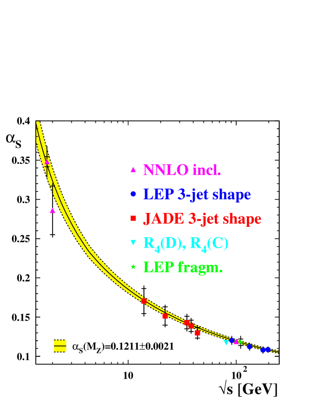
Figure 23: Values of $\alpha_{\mathrm{S}}$ determined at cms energy $\sqrt{s}$ from various processes as indicated. The NNLO incl. data are from $R_{\tau}$($m_{\tau}$), $R_{\mathrm{e^{+}e^{-}}}$(2 GeV) and the $\mathrm{Z^{0}}$ line shape observables. The error bars give experimental and total uncertainties. Invisible error bars are smaller than the symbols. The measurements at $\sqrt{s}\simeq m_{\mathrm{Z^{0}}}$ have been separated horizontally for clarity. The lines and shaded band show the running of the strong coupling based on the average value shown in equation (58).

8 Quark and gluon jets

Differences between the properties of jets originating from quarks or gluons are a basic consequence of QCD. The quarks and gluons can be viewed as carriers of colour charges given by their colour factors which are $C_{F}=4/3$ for quarks and $C_{A}=3$ for gluons. Predictions for e.g. the ratio of parton multiplicities

$$\frac{\mbox{$\langle n\rangle$}_{g}}{\mbox{$\langle n\rangle$}_{q}}=\frac{C_{A}}{C_{F}}$$ (59)

in jets originating from hard gluons or quarks [300, 301] can be related to observed quantities like charged hadron multiplicities measured in experimentally identified quark or gluon jets by assuming local parton hadron duality [64]. One therefore expects the particle multiplicities in gluon jets to be larger than in comparable quark jets.

With the relations $\mbox{$\langle x\rangle$}_{p}\mbox{$\langle n\rangle$}_{p}=1,p=q,g$, where $x=p_{\mathrm{parton}}/p_{\mathrm{jet}}$ is the scaled momentum of a parton produced in a quark or gluon jet and $\mbox{$\langle n\rangle$}_{p}$ is the parton multiplicity in the jet, one gets $\mbox{$\langle x\rangle$}_{q}/\mbox{$\langle x\rangle$}_{g}=C_{A}/C_{F}$. Thus gluon jets can be expected to have a softer scaled hadron momentum spectrum (fragmentation function) compared to quark jets of the same energy [301]. The tails at large $x\simeq 1$ of the fragmentation functions in gluon or quark jets can be predicted to have a ratio $\sim(1-x)/\ln(1-x)$ [301]. This implies that the gluon jet fragmentation function is expected to be softer by a factor of approximately $1-x$.

In experimental studies of differences between jets stemming from hard quarks or gluons the main difficulty lies in achieving a clear and unambiguous identification of the original parton. Due to the confinement property of QCD free partons are not observed but instead they form more or less collimated showers of softer partons and in turn of hadrons. This may cause a loss of the close correspondence between the hadronic final state and the underlying hard parton state. In addition the correlated colour flow between the quarks and gluons leads to effects of colour coherence with the consequence that the properties of gluon jets depend on the topology of the state in which they were produced, see e.g. [302].

Most theoretical predictions of differences between e.g. the average multiplicity of charged hadrons $\langle n_{\mathrm{ch.}}\rangle$ in quark or gluon jets don’t take experimental definitions of jets into account [303]. The jets are simply defined as $\mathrm{q\mathrm{\overline{q}}}$ or gg systems produced from a colour singlet point source. Hadronic final states in $\mathrm{e^{+}e^{-}}$ annihilation are a source of $\mathrm{q\mathrm{\overline{q}}}$ systems but gg systems from a colour singlet point source rarely occur in nature, the decay Y(3S)$\rightarrow\gamma\chi(2P)_{b,J=0,2}$, $\chi(2P)_{b,J=0,2}\rightarrow$gg [304] or production via 2-photon interactions [305] being examples. This prevents a clean interpretation of the experimental results based on jet finding algorithms to define jets and thus experimental techniques matching the theory more closely had to be found.

The next sections describe results obtained using exclusively defined jets employing jet finding algorithms and results based on inclusive jet definitions without involvement of jet finding algorithms.

8.1 Exclusive jets in 3-jet events

The first analysis showing significant differences between quark and gluon jets used LEP data from the $\mathrm{Z^{0}}$ peak and a novel technique to obtain clean samples of quark and gluon jets of the same energies [306]. The method [307] employs lepton tagging of quark jets in one-fold symmetric 3-jet events, so-called Y-events. The selection demands the angles between the highest energy jet and the other two jets to be within $150^{\mathrm{o}}\pm 10^{\mathrm{o}}$ yielding jet energies of about 24 GeV for the lower energy jets. The presence of a high momentum lepton (electron or muon) is required in one of the two lower energy jets. Since most such leptons stem from weak heavy quark decays the corresponding jet is identified as a quark jet. The production of heavy quark pairs from gluons of the perturbative cascade contributes ($3.1\pm 0.4$)% to c and ($0.27\pm 0.05$)% to b production and is thus a small effect (see section 5.5). The most energetic jet is also a quark jet with high probability due to the bremsstrahlung nature of hard gluon radiation and thus the remaining jet is likely to be a gluon jet. The selection of a second event sample requiring the same selection criteria except the lepton tagging allows to correct measurements of quark jet properties for a possible lepton tagging bias. The gluon jets are assumed to be unbiased.

Figure 24: (left) (a) Scaled energy spectrum of particles from quark (points) or gluon (line) jet cores. The solid points are corrected for the tagging bias. (b) Ratio of gluon to corrected quark jet data of (a). The lines in (b) are predictions from JETSET 7.2. (right) (a) and (c) Multiplicity spectrum as a function of the angle in the event plane $\psi$ for quark (points) and gluon (line) jets on a linear or logarithmic scale. The solid points are corrected for the tagging bias. The angle $\psi$ runs for points on the quark jet side and for the line on the gluon jet side. (b) Gluon/quark jet ratio of the data in (a) and (c). All figures from [306].

The main results of the analysis are summarised in figure 24. On the left in (a) the scaled energy spectrum of particles in the cores of the quark or gluon jets is shown where the open (solid) points represent the data after lepton tagging (after lepton tagging and bias correction). The line displays the result for gluon jets. The jet cores are defined as the angular region $135^{\mathrm{o}}<\psi<165^{\mathrm{o}}$ where $\psi$ is the angle in the event plane w.r.t. the highest energy jet. In left (b) the ratio of the bias corrected quark to the gluon jet data is given. The plots show convincing evidence for a softer scaled energy spectrum in gluon jets, as predicted. On the right in (a) and (c) the multiplicity spectrum obtained in quark (points) and gluon (line) jets is presented as a function of the angle $\psi$. The open and solid points are defined as above. The angle $\psi$ runs on the quark jet side of the event plane for points and on the gluon jet side for the line. Figure (b) on the right shows the gluon/quark jet ratio for $112.5^{\mathrm{o}}<\psi<180^{\mathrm{o}}$. The figures show evidence for a broader particle distribution in gluon jets compared to quark jets. The discrepancy visible in (c) in the region between jets is a manifestation of the string effect, see e.g. [308].

In a similar analysis using the same technique of lepton tagging of quark jets in 3-jet events the OPAL collaboration studied distributions of electric charge in quark and gluon jets [309]. The electric charge of a jet is defined by the sum $Q$ of charges of all charged particles assigned to the jet. The distributions of $Q$ filled separately for events with a positive or negative lepton tag are observed to have mean values significantly different from zero for the tagged and the highest energy jet. The $Q$ distribution for gluon jets has a mean value consistent with zero. The signs of the quark jet $Q$ distribution mean values correspond to the expected charge of the primary quark or antiquark. This observation constitutes experimental evidence based on $\mathrm{e^{+}e^{-}}$ data that gluons don’t have electric charge.

These analyses have been refined in several ways. The use of vertex instead of lepton tagging of heavy quarks employs that the decay vertex of heavy hadrons can be reconstructed using micro-vertex detectors. The technique uses a larger fraction of heavy hadron decays and allows better efficiencies and purities. The use of alternative jet finding algorithms like the cone [186] or the JADE algorithm quantified the influence of the jet reconstruction method on the results [310, 311], in particular the ratio of average charged particle multiplicities in quark and gluon jets at 24 GeV jet energy was found to be biased by about 10%. A different correction method ($\mathrm{q\mathrm{\overline{q}}}$g/$\gamma$) uses hadronic events consisting of two jets and one isolated and energetic photon as a pure sample of quark jets [311]. This method allows analysis of quark and gluon jets at varying energies finding e.g. that the ratio of charged particle multiplicities in gluon and quark jets depends on the jet energy.

A direct comparison of quark jets originating from light (u, d or s) or b quarks with gluon jets was performed by tagging the high energy jets of the one-fold symmetric samples [73, 312]. Vertex tagging is used to select b jets while the absence of charged particle tracks with large positive impact parameter indicates light quarks. Comparing the gluon jet tagged sample (vertex tag in a lower energy jet) with the light or b tagged sample (impact parameter or vertex tag in the high energy jet) allows to extract the properties of pure gluon, light or b jets at jet energies of about 24 GeV. Some results for the ratios of charged particle multiplicities are shown in table 13.

Table 13: Ratios of charged particle multiplicities of gluon and inclusive quarks ($R_{\mathrm{g/q}}$), gluon and light quarks ($R_{\mathrm{g/uds}}$) or gluon and b quark jets ($R_{\mathrm{g/b}}$) at $\sim 24$ GeV jet energy based on the Durham, JADE or the Cone algorithm. The methods “Y” and “$\mathrm{q\mathrm{\overline{q}}}$g/$\gamma$” refer to the analysis methods based on one-fold symmetric Y-events or $\mathrm{q\mathrm{\overline{q}}}$g and $\mathrm{q\mathrm{\overline{q}}}$$\gamma$ events to obtain results for pure quark and gluon jet samples from the data.

• Jet alg.	$y_{\mathrm{cut}}$	method	refs.	$R_{\mathrm{g/q}}$	$R_{\mathrm{g/uds}}$	$R_{\mathrm{g/b}}$
  Durham	0.01	Y	[312]	$1.19\pm 0.03$	$1.25\pm 0.09$	$1.06\pm 0.05$
  Durham	0.02	Y	[310, 73]	$1.25\pm 0.04$	$1.39\pm 0.05$	$1.09\pm 0.03$
  Durham	0.015	Y	[311]	$1.25\pm 0.04$	–	–
  Durham	0.01	$\mathrm{q\mathrm{\overline{q}}}$g/$\gamma$	[311]	$1.24\pm 0.06$	–	–
  JADE	0.04	$\mathrm{q\mathrm{\overline{q}}}$g/$\gamma$	[311]	$1.35\pm 0.08$	–	–
  Cone	–	Y	[310, 73]	$1.10\pm 0.03$	$1.14\pm 0.04$	$0.92\pm 0.04$

The multiplicity ratios $R_{\mathrm{g/q}}$ and $R_{\mathrm{g/uds}}$ are significantly larger than one in all cases proving that the charged particle multiplicity is greater in gluon than in quark jets. However, the difference between the ratios $R_{\mathrm{g/q}}$ and $R_{\mathrm{g/uds}}$ based on the different jet finding algorithms (Durham, JADE or Cone) implies that the results cannot be compared directly to QCD predictions [303, 73]. The values of $R_{\mathrm{g/b}}$ show that at jet energies of $\sim 24$ GeV the multiplicities of gluon and b jets are comparable.

Figure 25 (left) [73] shows the differential energy profile $\phi_{E}(r/R)=\Delta E/\Delta(r/R)$ where $\Delta E$ is the energy contained in an annulus of width $\Delta(r/R)$ at half angle $r$ aligned with the axis of the Cone jet with half angle $R$. A broader energy profile of gluon compared to light quark jets is clearly visible. The energy profile of b jets at $\sim 24$ GeV jet energy turns out be comparable to the gluon jet profile. Figure 25 (right) [73] presents the fragmentation function (FF) of charged particles. The gluon FF is clearly softer than the light quark (uds) FF, but the b quark FF is again observed to be similar to the gluon jet FF at jet energies of about 24 GeV.

Figure 25: (left) Comparison of b, uds and inclusive quark jets and gluon jets using the cone jet algorithm for the differential energy profile $\phi_{E}(r/R$, see text. (right) Comparison of the same b, uds and inclusive quark jets and gluon jets for the charged particle fragmentation function. All error bars show statistical uncertainties. Both figures from [73].

All studies discussed so far did not take into account the topology dependence of jet properties, see e.g. [45], because with symmetric 3-jet events the effects of topology dependence are suppressed. The topology dependence of particle multiplicity in jets in 3-jet configurations has been studied theoretically in detail, see e.g. [313] and references therein.

In the MLLA the total particle multiplicity of 3-jet events $N_{\mathrm{q\mathrm{\overline{q}}g}}(s,p_{\perp})$ produced at cms energies $\sqrt{s}$ also depends on the transverse momentum $p_{\perp}$ of the gluon jet, due to colour coherence [314, 45]. The quantity $N_{\mathrm{q\mathrm{\overline{q}}g}}$ is expressed as a sum of particle multiplicities in biased $\mathrm{q\mathrm{\overline{q}}}$ events $\hat{N}_{\mathrm{q\mathrm{\overline{q}}}}(s,p_{\perp})$ and in ideal and unbiased gg events $N_{\mathrm{gg}}(p_{\perp})$ taken at appropriate scales [315, 313]:

$$N_{\mathrm{q\mathrm{\overline{q}}g}}(s)=\hat{N}_{\mathrm{q\mathrm{\overline{q}}}}(L,p_{\perp,Lu})+\frac{1}{2}N_{gg}(p_{\perp,Lu})$$ (60)

with $L=\ln(s/\Lambda_{\mathrm{QCD}}^{2})$. The contribution $\hat{N}_{\mathrm{q\mathrm{\overline{q}}}}(L,p_{\perp})$ carries an explicit dependence on the gluon jet scale $p_{\perp}$ which relates it to the unbiased particle multiplicity $N_{\mathrm{q\mathrm{\overline{q}}}}$ measured without jet requirements [315]:

$$\hat{N}_{\mathrm{q\mathrm{\overline{q}}}}(L,p_{\perp})=N_{\mathrm{q\mathrm{\overline{q}}}}(L^{\prime})+(L-L^{\prime})\frac{\mathrm{d}N_{\mathrm{q\mathrm{\overline{q}}}}(L^{\prime})}{\mathrm{d}L}\;\;,$$ (61)

with $L^{\prime}=2\ln(p_{\perp}/\Lambda_{\mathrm{QCD}})+3/2)$. The transverse momentum of the gluon jet is defined by $p_{\perp,Lu}=\sqrt{s_{\mathrm{qg}}s_{\mathrm{\overline{q}}g}/s}$ with $s_{\mathrm{qg}}$ and $s_{\mathrm{\overline{q}}\mathrm{g}}$ the invariant masses in the qg and $\mathrm{\overline{q}}$g systems. In an alternative expression for $N_{\mathrm{q\mathrm{\overline{q}}g}}$ the variable $L$ is replaced by $L_{\mathrm{q\mathrm{\overline{q}}}}=\ln(s_{\mathrm{q\mathrm{\overline{q}}}}/\Lambda_{\mathrm{QCD}}^{2})$ and $p_{\perp,Lu}$ is replaced by $p_{\perp,Le}=\sqrt{s_{\mathrm{qg}}s_{\mathrm{\overline{q}}g}/s_{\mathrm{q\mathrm{\overline{q}}}}}$ [314, 45].

These predictions are only valid for 3-jet events selected without a cut on a fixed value of the jet resolution parameter $y_{\mathrm{cut}}$, since such a cut introduces an upper limit on the transverse momenta of any subjets. In contrast, when three jets are reconstructed in all events and the events are classified by the $p_{\perp}$ of the third jet the only remaining bias is given by the limitation of subjet transverse momenta. This bias is taken into account by the quantity $\hat{N}_{\mathrm{q\mathrm{\overline{q}}}}$ discussed above. Also, the jet reconstruction should be done using a jet resolution definition based on transverse momentum, e.g. the Durham, Cambridge or LUCLUS/PYCLUS algorithms.

For 3-fold symmetric 3-jet events with all three angles between the jets $\simeq 120$^o, so called Mercedes events, the alternative expression discussed above for the transverse momentum of the gluon jet simplifies [314, 45]:

$$p_{\perp,Le}=\sqrt{\frac{s_{\mathrm{qg}}s_{\mathrm{\overline{q}}\mathrm{g}}}{s_{\mathrm{q\mathrm{\overline{q}}}}}}\sim\frac{\sqrt{s}}{3}\sin\frac{\Theta}{2}\;\;.$$ (62)

This has been used as a motivation in experimental studies to use gluon and quark jet scales $Q_{\mathrm{jet}}=E_{\mathrm{jet}}\sin(\Theta/2)$ where $\Theta$ is the angle to the closest jet and thus takes the event topology into account [316, 317, 318, 319]. The study [316] showed that using $Q_{\mathrm{jet}}$ for quark jets and $\overline{Q}_{\mathrm{jet}}=\sqrt{Q_{\mathrm{qg}}Q_{\mathrm{\overline{q}}\mathrm{g}}}$ removes biases in the jet multiplicities which appear when jets with similar energies $E_{\mathrm{jet}}$ but at different angles $\Theta$ are compared.

The theoretical description of multiplicity in 3-jet events of equations (60) and (61) has been tested. In [320] the charged particle multiplicity in 2-jet events selected with the Durham jet algorithm with fixed vales of $y_{\mathrm{cut}}$ has been measured. The measurements have been compared with equation (61) using the relation $p_{\perp}=E_{\mathrm{vis}}\sqrt{y_{\mathrm{cut}}}$ and reasonable agreement within the total uncertainties of the data has been observed. Based on this result the charged particle multiplicity in unbiased gg events has been extracted as a function of the jet energy scale $Q$. The results are shown in figures 26 (a) and (b). In figure 26 (a) the measured $\hat{N}_{\mathrm{q\mathrm{\overline{q}}}}(L,p_{\perp})$ have been used to extract $N_{\mathrm{gg}}$ shown by the solid points at $Q=p_{\perp}$. The measurement of $N_{\mathrm{gg}}$ is compared with a pQCD prediction [321] which has been fitted to the data (solid line) and predictions by Monte Carlo simulations (dashed and dash-dotted lines) of artificial gg events. The predictions are found to agree well with the data including other measurements from inclusively defined gluon jets shown by solid triangles (see below). In figure 26 (b) the $\hat{N}_{\mathrm{q\mathrm{\overline{q}}}}(J,p_{\perp})$ have been calculated using equation (61) using both definitions of $p_{\perp}$; stars correspond to $p_{\perp,Lu}$ and $J=L$ and open points to $p_{\perp,Le}$ and $J=L_{\mathrm{q\mathrm{\overline{q}}}}$. The Monte Carlo predictions and inclusive gluon jet data are the same as in figure 26 (a). The results based on $p_{\perp,Lu}$ are in better agreement with the inclusive gluon jet data at lower and higher $Q$ than the results employing $p_{\perp,Le}$ as the jet energy scale.

Figure 26: (a) Results for $N_{\mathrm{gg}}$ shown by solid points as function of the jet energy scale $Q$ based on measured $\hat{N}_{\mathrm{q\mathrm{\overline{q}}}}(L^{\prime},p_{\perp})$ [320]. The error bars indicate total uncertainties. (b) Results for $N_{\mathrm{gg}}$ based on calculated $\hat{N}_{\mathrm{q\mathrm{\overline{q}}}}(L^{\prime},p_{\perp})$ using $p_{\perp,Lu}$ (stars) or $p_{\perp,Le}$ (open points). Both figures show by the solid and dashed or dash-dotted lines the same predictions from pQCD and Monte Carlo simulations and by the solid triangles other measurements based on inclusive gluon jets [320].

The quantities $N_{\mathrm{gg}}$ for gluon jets and $N_{\mathrm{q\mathrm{\overline{q}}}}$ for quark jets in two-parton systems are related by $\mathrm{d}N_{\mathrm{gg}}(L^{\prime})/\mathrm{d}L=C_{A}/C_{F}(1-\alpha_{0}c_{r}/L)\mathrm{d}N_{\mathrm{q\mathrm{\overline{q}}}}(L)/\mathrm{d}L$ with $\alpha_{0}=6C_{A}/(11C_{A}-2n_{f})$ and $c_{r}=10\pi^{2}/27-3/2$ [315]. The measurements of $N_{\mathrm{gg}}$ together with measured $N_{\mathrm{\mathrm{q\mathrm{\overline{q}}}}}$ thus allow a precise determination of ratio of colour factors $C_{A}/C_{F}$ [320]:

$$C_{A}/C_{F}=2.23\pm 0.01\mathrm{(stat.)}\pm 0.14\mathrm{(syst.)}$$ (63)

The data in figure 26 (a) above $Q=7$ GeV have been used in the fit and the fit result corresponds to the solid line. In[318] a similar measurement has been performed for the first time using slightly different predictions [235] and involving an additional non-perturbative correction. The result was $C_{A}/C_{F}=2.25\pm 0.06\mathrm{(stat.)}\pm 0.12\mathrm{(syst.)}$. Both results for $C_{A}/C_{F}$ agree well with the QCD expectation of $C_{A}/C_{F}=2.25$ and have small systematic uncertainties compared to other measurements of this quantity. A compilation of other measurements of $C_{A}/C_{F}$ is shown in section 9.

The FFs of quark and gluon jets in mirror symmetric Y-events and completely symmetric Mercedes events were studied as function of the scaled jet energy $Q_{\mathrm{jet}}$ [317]. The comparison of the gluon FF in Y and Mercedes events found evidence for scaling violations in the gluon FF. The scaling violation of the gluon jet FF was seen to be stronger than the comparable quark jet FF consistent with the QCD expectation motivated by the larger colour charge of gluons compared to quarks. This observation was confirmed by a study of subjets in quark and gluon jets. To find subjets the jet finding algorithm is run only on the particles associated with the gluon or quark jet [317]. The fraction of events without subjet production was found to be smaller in the quark jet sample in agreement with the expectation and an NLLA QCD calculation.

Other subjects of study have been the production rates of identified particles in quark and gluon jets. In several analyses the production of $\pi^{0}$ and $\eta$ [322, 319], of $\mathrm{K_{S}^{0}}$ [323, 324, 325, 319], $\mathrm{K^{+}}$ and p [324], and $\Lambda^{0}$ [325, 324, 323] was investigated. In [322] the production of $\pi^{0}$ and $\eta$ was measured in 2- and 3-jet events and $\eta$ production was found to increase stronger than $\pi^{0}$ production in 3-jet events. This observation was not confirmed in [319] where production rates of $\pi^{0}$, $\eta$ and $\mathrm{K_{S}^{0}}$ in gluon jets were found to be larger than in quark jets by the same factor as for the increase of the inclusive charged particle multiplicity. In [324] it was observed that the momentum spectra of $\mathrm{K_{S}^{0}}$, $\mathrm{K^{+}}$, p and $\Lambda^{0}$ were softer in gluon compared to quark jets with a higher total particle multiplicity.

8.2 Inclusive jets

In the definition of inclusive gluon and quark jets no jet finding algorithm is directly involved. This removes systematic uncertainties connected with the assignment of particles to jets, as discussed in the previous section. Studies using inclusive gluon jets are based on i) particle decays to hadronic final states via gluons only [304, 326] or ii) $\mathrm{e^{+}e^{-}}\rightarrow\mathrm{q\mathrm{\overline{q}}g}$ events at high energy in the rare kinematic configuration where a hard gluon g recoils against the $\mathrm{q\mathrm{\overline{q}}}$ system [303].

The first study using inclusive gluon jets was [304] using the decays Y(3S)$\rightarrow\gamma\chi_{b}(2P)$, Y(1S)$\rightarrow$ggg, and $\mathrm{q\mathrm{\overline{q}}}$ events produced in the continuum at $\sqrt{s}=10.55$ GeV. The $\chi_{b}(2P)$ states with $J=0,2$ can decay to gg while the $\chi_{b}(2P),J=1$ state decays to $\mathrm{q\mathrm{\overline{q}}g}$. The three different $\chi_{b}(2P),J=0,1,2$ states are disentangled employing their slightly differing invariant masses. The distributions of the event shape observable $R_{2}$ derived from $\chi_{b}(2P),J=0,2$ decays or continuum events evolved to the $\chi_{b}(2P),J=1$ scale show clear differences.

In a similar study [326] events of the type $\mathrm{Y(1S)}\rightarrow\mathrm{gg}\gamma$ are compared with $\mathrm{e^{+}e^{-}}\rightarrow\mathrm{q\mathrm{\overline{q}}}\gamma$ events produced in the continuum. The mean charged particle multiplicity is measured in both samples as a function of the recoil mass of the photon. The ratio of multiplicities in gg and $\mathrm{q\mathrm{\overline{q}}}$ systems for recoil masses below 7 GeV is found to be compatible with unity. The gluon multiplicities are also shown in figures 26 (a) and (b).

A method to obtain inclusive gluon jets at high energy has been proposed in [303]. The inclusive gluon jet definition is achieved experimentally by selecting hadronic $\mathrm{Z^{0}}$ decays were both q and $\mathrm{\overline{q}}$ are detected in the same hemisphere of the event. The quarks are identified via tagging of heavy quark decays and the gluon jet is identified with the other hemisphere of the event. In two studies the mean charged particle multiplicity [328] and the charged particle multiplicity distributions [329] were measured in inclusive gluon and quark jets. The multiplicity distribution was analysed in terms of higher moments and agreement with a NNLO QCD calculation was found for gluon and quark jets. The latest result for the ratio of mean charged particle multiplicities in inclusive quark and gluon jets of $E_{\mathrm{jet}}=40.1$ GeV is $r_{ch}=1.51\pm 0.02\mathrm{(stat.)}\pm 0.03\mathrm{(syst.)}$ [330]. This is only in qualitative agreement with results from exclusive jets discussed in the previous section.

Figure 27: Ratio of scaled momentum distributions of charged particles measured in inclusive gluon and quark jets at $E_{\mathrm{jet}}=40.1$ GeV. Superimposed are fits of the form $(1-x)/\ln(1-x)$ as predicted in [301]. The DELPHI data points are horizontally displaced for clarity. Data from [317, 330, 331].

In [330] many properties of inclusive gluon and quark jets at high jet energies were studied. The measurement of the distributions of charged particle energy fractions $x_{E}$ allows to test some of the predictions discussed above. From the data for $x_{E}$ in table 2 of [330] one can extract $\mbox{$\langle x_{E}\rangle$}_{g}=0.044\pm 0.002$, $\mbox{$\langle x_{E}\rangle$}_{q}=0.0635\pm 0.0003$. The ratio is found as

$$r_{\mbox{$\langle x\rangle$}}=\mbox{$\langle x_{E}\rangle$}_{q}/\mbox{$\langle x_{E}\rangle$}_{g}=1.44\pm 0.07\;\;,$$ (64)

where the error contains an additional contribution of 3% to cover the energy difference between the inclusive gluon jets at 40.1 GeV and the quark jets at 45.6 GeV. The result for $r_{\mbox{$\langle x\rangle$}}$ is consistent with the result for $r_{ch}$ shown above. The prediction of [301] discussed above for the behaviour of the ratio of $x_{E}$ distributions can be tested by fitting a function $a(1-x)/\ln(1-x)+b$, where $a$ and $b$ free parameters, to the data for $x_{E}>0.2$. Figure 27 presents the results of such fits using the data of [317, 330, 331]. The fits based on the total errors agree with the data; the results are shown in table 14. The fit to OPAL data was performed with $b=0.0$ fixed since the fitted value of $b$ was consistent with zero.

Table 14: Results of fits of $a(1-x)/\ln(1-x)+b$ as explained in the text to data for ratios of FFs from gluon and quark jets.

• 	a	b	$\chi^{2}/\mathrm{d.o.f.}$
  ALEPH $y_{\mathrm{cut}}=0.1$	$0.176\pm 0.064$	$0.36\pm 0.11$	0.03/1
  DELPHI Merc.	$0.267\pm 0.033$	$0.067\pm 0.057$	4.3/4
  DELPHI Y	$0.306\pm 0.010$	$0.124\pm 0.014$	25/5
  OPAL $g_{incl}$	$0.218\pm 0.035$	0.0 (fixed)	1.3/6

The results for $a$ can be averaged yielding $\bar{a}=0.295\pm 0.009$ with a $\chi^{2}/\mathrm{d.o.f.}=10/3$. The data qualitatively support the prediction of [301]. However, there are significant differences between the fit results indicating substantial systematic differences between the different data sets, which have been obtained using different experimental techniques.

9 QCD gauge structure

QCD as the gauge theory of strong interactions assumes that quarks carry one out of three strong charges, referred to as colour. The requirement of local gauge symmetry under SU(3) transformations in the colour space generates the gauge bosons of QCD: an octet of gluons each carrying colour charge and anti-charge, see e.g. [5]. The gluons can thus interact with themselves; it is due to this property of the QCD gauge bosons that the theory explains confinement and asymptotic freedom via the running of the strong coupling $\alpha_{\mathrm{S}}$.

In perturbative QCD at NLO three fundamental vertices contribute: i) the quark-gluon vertex with colour factor $C_{F}$, ii) the gluon-gluon vertex with colour factor $C_{A}$ and iii) the $\mathrm{q\mathrm{\overline{q}}}$ production from a gluon with colour factor $T_{F}n_{f}$, see e.g. [332]. The colour factors are $C_{F}=4/3$, $C_{A}=3$ and $T_{F}n_{f}=1/2\cdot 5$ in QCD with SU(3) gauge symmetry and specify the relative contribution of the corresponding vertex to observables. In NLO QCD the prediction for an observable $R$ is $R=A\alpha_{\mathrm{S}}+(B_{C_{F}}C_{F}+B_{C_{A}}C_{A}+B_{T_{F}}T_{F}n_{f})C_{F}\alpha_{\mathrm{S}}^{2}$; NLLA predictions e.g. for event shapes or jet rates decompose in a similar way. For NLO predictions for 4-jet observables an analogous decomposition in terms of the six possible products of two out of the three colour factors holds [7]; a seventh term is negligible and left out.

Experimental investigations of the gauge structure of QCD are possible because of the different angular momenta in the initial and final states of the fundamental vertices. It is an important test of QCD to probe the gauge structure in experiments. Several techniques with rather different experimental and theoretical uncertainties have been developed; we will discuss here some recent results.

9.1 Four-jet events

The LEP experiments ALEPH [181] and OPAL [185] have analysed 4-jet final states from hadronic $\mathrm{Z^{0}}$ decays using the recent QCD NLO predictions (see e.g. [7] and references therein). The 4-jet final states are selected by clustering events using the Durham algorithm [169] with $y_{\mathrm{cut}}=0.008$ and demanding four jets. At this value of $y_{\mathrm{cut}}$ the 4-jet fraction is relatively large ($\mathrm{R}_{4}\simeq 7$%) and the four jets are well separated.

The energy-ordered 4-momenta $p_{i},i=1,\ldots,4$ of the jets are used to calculate the angular correlation observables (see [181, 185] for details). As an example, the Bengtsson-Zerwas angle $\chi_{\mathrm{BZ}}$ is defined by [183] $\chi_{\mathrm{BZ}}=\angle([\vec{p}_{1}\times\vec{p}_{2}],[\vec{p}_{3}\times\vec{p}_{4}])$, i.e. the angle between the two planes spanned by the momentum vector pairs $(\vec{p}_{1},\vec{p}_{2})$ and $(\vec{p}_{3},\vec{p}_{4})$. Assuming that energy ordering selected the primary quarks from the $\mathrm{Z^{0}}$ decay as $(p_{1},p_{2})$ the observable $\chi_{\mathrm{BZ}}$ is sensitive to the decay of an intermediate gluon to gluons (vertex ii)) or quarks (vertex iii)) and the competing process of radiation of a second gluon from a primary quark (vertex i)).

Figure 28 (left) presents the uncorrected distribution of $\cos(\chi_{\mathrm{BZ}})$ measured by ALEPH [181]. Superimposed on the data points is the result of a simultaneous fit of the NLO QCD predictions to four angular correlations including $\chi_{\mathrm{BZ}}$ and the distribution of the 4-jet rate $\mathrm{R}_{4}$. From the fit values for $\alpha_{\mathrm{S}}(m_{\mathrm{Z^{0}}})$ and the colour factors $C_{A}$ and $C_{F}$ are extracted. The results from ALEPH are $\alpha_{\mathrm{S}}(m_{\mathrm{Z^{0}}})=0.119\pm 0.027$, $C_{A}=2.93\pm 0.60$ and $C_{F}=1.35\pm 0.27$; from OPAL we have $\alpha_{\mathrm{S}}(m_{\mathrm{Z^{0}}})=0.120\pm 0.023$, $C_{A}=3.02\pm 0.55$ and $C_{F}=1.34\pm 0.26$. The systematic errors are dominated by uncertainties from the hadronisation corrections and theoretical errors from estimating missing higher order contributions. The hadronisation corrections are implemented using Monte Carlo models with standard values for the colour factors. Both analyses use an unconventional method of estimating systematic uncertainties. A more conservative evaluation based on the information available in [181, 185] leads to total errors for $\alpha_{\mathrm{S}}(m_{\mathrm{Z^{0}}})$, $C_{A}$ and $C_{F}$ of $\pm 0.048$, $\pm 1.06$ and $\pm 0.46$ for ALEPH and $\pm 0.049$, $\pm 1.07$ and $\pm 0.47$ for OPAL; i.e. the errors turn out to be approximately twice as large.

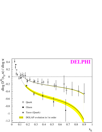
Figure 28: (left) Distribution of $|\cos\chi_{\mathrm{BZ}}|$ before corrections (solid points). Superimposed is a fit of NLO QCD (solid lines) [181]. (right) Measurements of $\mathrm{d}D^{H}(x_{\mathrm{E}},\kappa_{\mathrm{H}})/\mathrm{d}\log(\kappa_{\mathrm{H}})$ for gluon (solid points) and quark jets (open circles and solid triangles). The lines represent a fit of the LO QCD prediction [333].

9.2 Scaling violation in gluon and quark jets

Jets originating from quarks or gluons should have different properties due to the different colour charge carried by quarks or gluons, see section 8. In an analysis by DELPHI [333] the scaling violation of the fragmentation function (FF) in gluon and quark jets at different energies is compared. From a sample of $3.7\cdot 10^{6}$ hadronic $\mathrm{Z^{0}}$ decays planar 3-jet events with well reconstructed jets are selected using the Durham or Cambridge algorithms, but without imposing a fixed value of $y_{\mathrm{cut}}$ in order to reduce biases [315] (see section 8.1) . In events with the two angles between the most energetic jet and the other jets in the range between 100^o and 170^o a b-tagging procedure is applied to the jets. Gluon jets are identified indirectly as the jets without a successful b-tag. Jets originating from light (udsc) quarks are taken from events which failed the b-tagging. A correction procedure based on efficiencies and purities determined by Monte Carlo simulation yields results for pure gluon or quark jets.

The jet energy scale is calculated according to $\kappa_{\mathrm{H}}=E_{\mathrm{jet}}\sin(\theta/2)$, where $\theta$ is the angle w.r.t. to the closest jet. This definition takes colour coherence effects into account [302]. The FF in a jet $D^{H}(x_{\mathrm{E}},\kappa_{\mathrm{H}})$ is given by the distribution of $x_{\mathrm{E}}=E_{\mathrm{hadron}}/\kappa_{\mathrm{H}}$ for the hadrons assigned to the jet. The evolution of the FFs of gluon and quark jets with jet energy scale $\kappa_{\mathrm{H}}$ is studied in intervals of $x_{\mathrm{E}}$. Figure 28 (right) presents the quantity $\mathrm{d}D^{H}(x_{\mathrm{E}},\kappa_{\mathrm{H}})/\mathrm{d}\log(\kappa_{\mathrm{H}})$, i.e. the slopes of the scaling violation for a given interval of $x_{\mathrm{E}}$, for quark and gluon jets. The steeper slopes corresponding to stronger scaling violations of gluon compared to quark jets are clearly visible. A fit of the scaling violations based on the LO QCD prediction (DGLAP equation) allows to extract the ratio $C_{A}/C_{F}$ resulting in $C_{A}/C_{F}=2.26\pm 0.16$.

9.3 Event shape fits

In this analysis [334] the decomposition of the $\mathcal{O}(\alpha_{\mathrm{S}}^{2})$+NLLA QCD predictions for event shape observables into terms proportional to the colour factors is used. Since the sensitivity of event shape distributions measured at LEP 1 alone is not sufficient [335] data from $\sqrt{s}=14$ to 189 GeV are used. In this way the colour structure of the running of the strong coupling contributes as well. Hadronisation corrections are implemented using power corrections, see section 4.5.1. The advantage of using power corrections instead of Monte Carlo model based hadronisation corrections is that the colour structure of the power corrections is known and can be varied in the fit.

In the analysis simultaneous fits of $\alpha_{\mathrm{S}}(m_{\mathrm{Z^{0}}})$, $C_{A}$ and $C_{F}$ to data for the event shape observables $1-T$ at $\sqrt{s}=14$ to 189 GeV and $C$ at $\sqrt{s}=35$ to 189 GeV are performed. The data for $1-T$ and $C$ are analysed separately and the results are combined. The results are $\alpha_{\mathrm{S}}(m_{\mathrm{Z^{0}}})=0.119\pm 0.010$, $C_{A}=2.84\pm 0.24$ and $C_{F}=1.29\pm 0.18$ and are shown on figure 29 below. The errors are dominated by uncertainties from the hadronisation correction and from experimental effects.

9.4 Colour factor averages

The measurements of the colour factors $C_{A}$ and $C_{F}$ or of $x=C_{A}/C_{F}$ discussed above or in section 8 can be combined into average values of $C_{A}$ and $C_{F}$ taking into account correlations between $C_{A}$ and $C_{F}$ as well as between different experiments. The variables $x$ and $y=T_{F}/C_{F}$ are used to define the $\chi^{2}$ function

$$\chi^{2} = \sum_{i}(x_{i}-\bar{x})v^{(xy)}_{i}(y_{i}-\bar{y})+$$

$$\sum_{ij}(x_{i}-\bar{x})v^{(x)}_{ij}(x_{j}-\bar{x})+$$

$$\sum_{ij}(y_{i}-\bar{y})v^{(y)}_{ij}(y_{j}-\bar{y})\;\;,$$

where $\bar{x}$ and $\bar{y}$ are the averages, the indices $i$ and $j$ count experiments, $v^{(xy)}_{i}$, $v^{(x)}_{ij}$ and $v^{(y)}_{ij}$ are elements of the inverses of the corresponding covariance matrices for the $x_{i}$ and $y_{i}$ within experiment $i$ and for the $x_{i}$ and $y_{i}$ between experiments. The averages $\bar{x}$ and $\bar{y}$ are converted to the average values $\overline{C}_{A}$ and $\overline{C}_{F}$ after the fit is performed. The input data for $x$ and $y$ are directly taken from [181, 185, 333, 320] while the results from [334] have to be converted.

The covariance matrices between experiments are constructed as follows: the ALEPH and OPAL 4-jet analyses have experimental and hadronisation errors partially and theory errors fully correlated, the 4-jet analyses and the event shape analysis have hadronisation errors partially and theory errors fully correlated, and the 4-jet and event shape analyses and the DELPHI FF and the OPAL $N^{\mathrm{ch.}}_{\mathrm{gg}}$ analyses have their theory errors partially correlated.

The averaging fit is done using only the first term of equation (9.4) to determine the averages $\overline{C}_{A}$ and $\overline{C}_{F}$ avoiding possible biases from our assumptions on correlations of systematic uncertainties between different sets of measurements. The fit is repeated using only statistical correlations in the first term to determine the statistical errors and using the full covariance matrix to determine the total errors. The final results are

$$\overline{C}_{A} = 2.89\pm 0.03\mathrm{(stat.)}\pm 0.21\mathrm{(syst.)}$$ (66)

$$\overline{C}_{F} = 1.30\pm 0.01\mathrm{(stat.)}\pm 0.09\mathrm{(syst.)}$$

with correlation coefficient $\rho=0.82$. The relative total uncertainties are about 8% for both $\overline{C}_{A}$ and $\overline{C}_{F}$. The fit using the full covariance matrix yields $\overline{C}_{A}=2.83$ and $\overline{C}_{F}=1.29$ in good agreement with our main results.

Figure 29 presents the results of the individual analysis in a $C_{F}$ vs. $C_{A}$ plane together with the combined result and the expectations of QCD based on the SU(3) gauge symmetry and various other gauge symmetries. The correlation coefficients for [181, 185] were calculated from the references with the results $\rho=0.97$ (ALEPH) and $\rho=0.93$ (OPAL). The error ellipses refer to 90% CL. The combined result is in good agreement with the individual analyses and with standard SU(3) QCD while the total uncertainties are substantially reduced. The other possibilities for gauge symmetries shown on the figure are clearly ruled out.

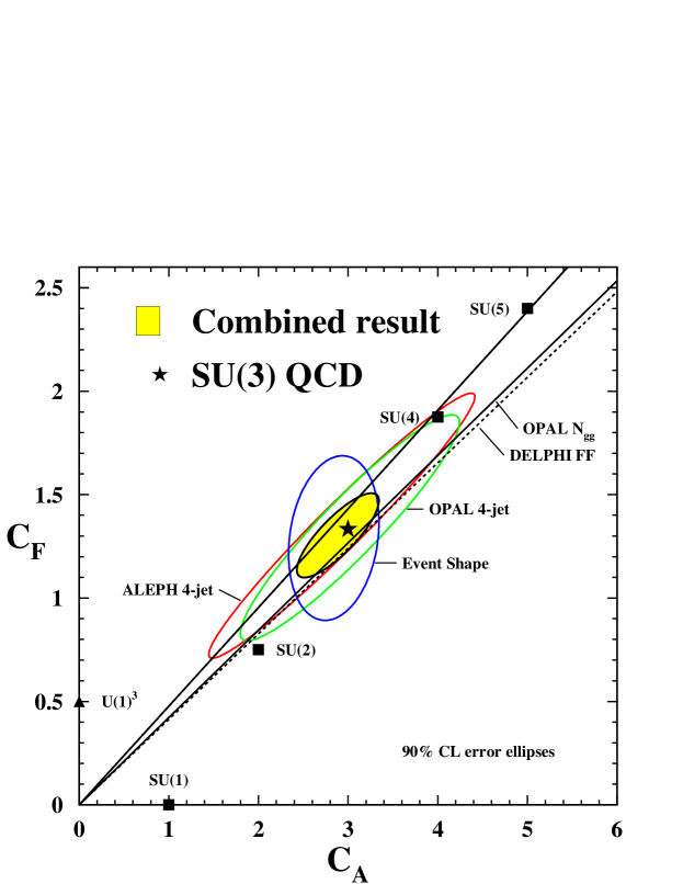
Figure 29: Measurements of the colour factors $C_{A}$ and $C_{F}$ discussed in this report. The ellipses show the correlated measurements using 4-jet events [181, 185] or event shape distributions [334] while the lines represent the results of determinations of $C_{A}/C_{F}$ from DELPHI [333] (dashed) and OPAL [320] (solid). The upper solid and dashed lines overlap. The grey filled ellipsis displays the combined result for $\overline{C}_{A}$ and $\overline{C}_{F}$ (see text). The solid triangle and squares show the expectations for various assumptions for the gauge symmetry of QCD as indicated on the figure.

10 Conclusions and outlook

We have shown in this report that hadron production in $\mathrm{e^{+}e^{-}}$ annihilation is a useful and fruitful environment to test the theory of strong interactions, QCD. The absence of interference between initial and final states and the large range of cms energies probed by the experiments make many stringent tests of the theory possible. The early results from hadron production in $\mathrm{e^{+}e^{-}}$ annihilation at low energies were crucial to establish QCD as the theory of strong interactions and thus as an integral part of the standard model of high energy physics.

Studies of differences between quark and gluon jets reveal many properties of the gauge bosons of QCD, the gluons, which are correctly predicted by the theory. The measurements of jet production rates and event shape observables using theoretically and experimentally well behaved observables allow direct tests of advanced perturbative QCD predictions and precise determinations of the value of the strong coupling constant $\alpha_{\mathrm{S}}$. A fundamental prediction by QCD is asymptotic freedom of the coupling at high energies and this has been verified directly using data over a large range of cms energies. More indirect tests of asymptotic freedom stem from successful comparison of precision determinations of $\alpha_{\mathrm{S}}$ at different energy scales.

The most reliable and precise determinations of $\alpha_{\mathrm{S}}$ in $\mathrm{e^{+}e^{-}}$ annihilation to hadrons employ inclusive observables such as the hadronic branching ratios of the gauge bosons of the electroweak theory, $\gamma$, $\mathrm{Z^{0}}$ and $\mathrm{W^{\pm}}$. The inclusive observables are mostly unaffected by hadronisation corrections and they are accessible to NNLO perturbative QCD calculations with 2-loop radiative corrections. The final result for $\alpha_{\mathrm{S}}(m_{\mathrm{Z^{0}}})$ from inclusive observables calculated in NNLO perturbative QCD is

$$\alpha_{\mathrm{S}}(m_{\mathrm{Z^{0}}})=0.1211\pm 0.0010\mathrm{(exp.)}\pm 0.0018\mathrm{(theo.)}\;\;.$$

This result is in good agreement with recent world averages of measurements of the strong coupling constant $\alpha_{\mathrm{S}}(m_{\mathrm{Z^{0}}})=0.1184\pm 0.0027$ [207] or $\alpha_{\mathrm{S}}(m_{\mathrm{Z^{0}}})=0.1187\pm 0.0020$ [18] which are based on all available analyses. The best measurements of $\alpha_{\mathrm{S}}(m_{\mathrm{Z^{0}}})$ including ours shown above yield errors of about 2%. The other determinations of $\alpha_{\mathrm{S}}$ discussed in this report are found to be in good agreement with our main result and we note that the results from analyses of the 4-jet rate using the Durham or Cambridge algorithms are of similar precision. Further improvements in the near future may be expected from NNLO calculations for 3-jet observables which are expected to reduce the otherwise dominating theoretical uncertainties and might allow total uncertainties of 1% [336].

Studies of the gauge structure of QCD using angular correlations in 4-jet final states, 3-jet observables at different energy scales and quark and gluon jet differences were discussed. The results for the colour factors $C_{A}$ and $C_{F}$ were observed to be in good agreement and combined values were calculated. The results are

$$C_{A} = 2.89\pm 0.03\mathrm{(stat.)}\pm 0.21\mathrm{(syst.)}$$

$$C_{F} = 1.30\pm 0.01\mathrm{(stat.)}\pm 0.09\mathrm{(syst.)}$$

with correlation $\rho=0.82$. These results are in good agreement with expectations from QCD with the SU(3) gauge symmetry $C_{A}=3$ and $C_{F}=4/3$.

In summary, $\mathrm{e^{+}e^{-}}$ annihilation to hadrons has been and still is indispensable to stringently probe the theory of strong interactions. QCD has been established as a part of the standard model of high energy physics and has been tested to a precision of 2% with some well suited observables. This impressive result has been achieved by the LEP experiments, SLD, the re-analysis of JADE data and the parallel theoretical work stimulated by the availability of precise data. Future high energy physics programmes such as the LHC or the ILC will benefit greatly from this achievement, because precise and reliable QCD predictions will be essential for disentangling possible new physics signals from standard processes.

11 References

References

- [1] Fritzsch H, Gell-Mann M and Leutwyler H 1973 Phys. Lett. B 47 365–368
- [2] Gross D J and Wilczek F 1973 Phys. Rev. Lett. 30 1343–1346
- [3] Gross D J and Wilczek F 1973 Phys. Rev. D 8 3633–3652
- [4] Politzer H D 1973 Phys. Rev. Lett. 30 1346–1349
- [5] Ellis R, Stirling W and Webber B 1996 QCD and Collider Physics vol 8 of Cambridge Monographs on Particle Physics, Nuclear Physics and Cosmology (Cambridge University Press)
- [6] Muta T 1987 Foundations of Quantum Chromo Dynamics vol 5 of World Scientific Lecture Notes in Physics (World Scientific)
- [7] Nagy Z and Trocsanyi Z 1998 Phys. Rev. D 57 5793–5802
- [8] Callan, Curtis G. J 1970 Phys. Rev. D 2 1541–1547
- [9] Symanzik K 1970 Commun. Math. Phys. 18 227–246
- [10] Grunberg G 1980 Phys. Lett. B 95 70
- [11] Grunberg G 1984 Phys. Rev. D 29 2315
- [12] Stevenson P M 1981 Phys. Rev. D 23 2916
- [13] Brodsky S J, Lepage G P and Mackenzie P B 1983 Phys. Rev. D 28 228
- [14] Dhar A and Gupta V 1984 Phys. Rev. D 29 2822
- [15] Chyla J and Kataev A L 1995 in Reports of the working group on precision calculations for the Z resonance ed Bardin Y, Passarino G and Hollik W (CERN 95-13) hep-ph/9502383
- [16] Stevenson P 1982 Nucl. Phys. B 203 472
- [17] Brodsky S J and Lu H J 1995 Phys. Rev. D 51 3652–3668
- [18] Particle Data Group Coll. Eidelman S et al 2004 Phys. Lett. B 592 1
- [19] Vermaseren J A M, Larin S A and van Ritbergen T 1997 Phys. Lett. B 405 327–333
- [20] Chetyrkin K G, Kniehl B A and Steinhauser M 1997 Phys. Rev. Lett. 79 2184–2187
- [21] Sterman G and Weinberg S 1977 Phys. Rev. Lett. 39 1436
- [22] Ellis R, Ross D and Terrano A 1981 Nucl. Phys. B 178 421
- [23] Kunszt Z and Nason P 1989 in Z physics at LEP 1 ed Altarelli G, Kleiss R and Verzegnassi C vol 1 (CERN 89-08)
- [24] Catani S and Seymour M 1996 Phys. Lett. B 378 287–301
- [25] Gehrmann-De Ridder A, Gehrmann T and Glover E W N 2004 Nucl. Phys. Proc. Suppl. 135 97–101
- [26] Ridder A G D, Gehrmann T and Glover E W N 2005 ZU-TH-07-05 hep-ph/0505111
- [27] Gorishnii S G, Kataev A L and Larin S A 1991 Phys. Lett. B 259 144–150
- [28] Nagy Z and Trocsanyi Z 1998 Phys. Rev. D 59 014020 Erratum-ibid.D62:099902,2000
- [29] Campbell J M, Cullen M A and Glover E W N 1999 Eur. Phys. J. C 9 245–265
- [30] Catani S, Trentadue L, Turnock G and Webber B R 1993 Nucl. Phys. B 407 3
- [31] Banfi A, Salam G P and Zanderighi G 2002 J. High Energy Phys. 01 018
- [32] Dokshitzer Y L, Lucenti A, Marchesini G and Salam G P 1998 J. High Energy Phys. 1 011
- [33] Catani S and Webber B R 1998 Phys. Lett. B 427 377–384
- [34] OPAL Coll. Acton P D et al 1993 Z. Phys. C 59 1–19
- [35] Dasgupta M and Salam G P 2004 J. Phys. G 30 R143
- [36] Surguladze L R and Samuel M A 1991 Phys. Rev. Lett. 66 560–563 erratum ibid. 2416
- [37] Chetyrkin K G 1997 Phys. Lett. B 391 402–412
- [38] James F 1980 Rept. Prog. Phys. 43 1145
- [39] Sjöstrand T 1989 in Z physics at LEP 1 ed Altarelli G, Kleiss R and Verzegnassi C vol 3 (CERN 89-08)
- [40] Knowles I and Sjöstrand T 1996 in Physics at LEP 2 ed Altarelli G, Sjöstrand T and Zwirner F vol 2 (CERN 96-01)
- [41] Webber B R 1986 Annu. Rev. Nucl. Part. Sci. 36 253
- [42] Gribov V N and Lipatov L N 1972 Sov. J. Nucl. Phys. 15 438–450
- [43] Altarelli G and Parisi G 1977 Nucl. Phys. B 126 298
- [44] Dokshitzer Y L 1977 Sov. Phys. JETP 46 641–653
- [45] Dokshitzer Y L, Khoze V A, Mueller A H and Troyan S I 1991 Basics of perturbative qcd (Editions Frontieres)
- [46] Bengtsson M and Sjöstrand T 1987 Phys. Lett. B 185 435
- [47] Seymour M H 1995 Comput. Phys. Commun. 90 95–101
- [48] Sjöstrand T, Lönnblad L and Mrenna S 2001 LU-TP-01-21 hep-ph/0108264
- [49] Corcella G et al 2001 J. High Energy Phys. 01 010
- [50] Gustafson G and Pettersson U 1988 Nucl. Phys. B 306 746
- [51] Andre J and Sjöstrand T 1998 Phys. Rev. D 57 5767–5772
- [52] Lonnblad L 2002 J. High Energy Phys. 05 046
- [53] Catani S, Krauss F, Kuhn R and Webber B R 2001 J. High Energy Phys. 11 063
- [54] Frixione S and Webber B R 2002 J. High Energy Phys. 06 029
- [55] Kurihara Y et al 2002 KEK-CP-121 hep-ph/0212216
- [56] Andersson B, Gustavson G, Ingelman G and Sjöstrand T 1983 Phys. Rep. 97 31
- [57] Andersson B, Gustafson G and Sjöstrand T 1985 Phys. Scripta 32 574
- [58] Peterson C, Schlatter D, Schmitt I and Zerwas P 1983 Phys. Rev. D 27 105
- [59] Gottschalk T D 1983 Nucl. Phys. B 214 201
- [60] Field R D and Wolfram S 1983 Nucl. Phys. B 213 65
- [61] Webber B R 1984 Nucl. Phys. B 238 492
- [62] Marchesini G and Webber B R 1988 Nucl. Phys. B 310 461
- [63] Amati D and Veneziano G 1979 Phys. Lett. B 83 87
- [64] Azimov Y I, Dokshitzer Y L, Khoze V A and Troian S I 1985 Z. Phys. C 27 65–72
- [65] Marchesini G and Webber B R 1990 Nucl. Phys. B 330 261
- [66] Lönnblad L 1992 Comput. Phys. Commun. 71 15–31
- [67] Odorico R 1984 Comput. Phys. Commun. 32 139
- [68] Mazzanti P and Odorico R 1993 Nucl. Phys. B 394 267
- [69] Field R D and Feynman R P 1978 Nucl. Phys. B 136 1
- [70] ALEPH Coll. Barate R et al 1998 Phys. Rep. 294 1
- [71] DELPHI Coll. Abreu P et al 1996 Z. Phys. C 73 11–60
- [72] L3 Coll. Achard P et al 2004 Phys. Rep. 399 71–174
- [73] OPAL Coll. Alexander G et al 1996 Z. Phys. C 69 543–560
- [74] OPAL Coll. Abbiendi G et al 2004 Eur. Phys. J. C 35 293–312
- [75] SLD Coll. Abe K et al 1997 Phys. Rev. Lett. 79 590–596
- [76] Salam G P and Wicke D 2001 J. High Energy Phys. 05 061
- [77] Beneke M and Braun V M 2001 in At the Frontier of Particle Physics/Handbook of QCD vol 3 pages 1719–1773 (World Scientific) hep-ph/0010208
- [78] Dokshitzer Y, Marchesini G and Webber B 1996 Nucl. Phys. B 469 93–142
- [79] Brodsky S J, Menke S, Merino C and Rathsman J 2003 Phys. Rev. D 67 055008
- [80] Dokshitzer Y L and Webber B R 1997 Phys. Lett. B 404 321–327
- [81] Dokshitzer Y L, Lucenti A, Marchesini G and Salam G P 1998 J. High Energy Phys. 5 003
- [82] Dokshitzer Y L, Marchesini G and Salam G P 1999 Eur. Phys. J. direct C 3 1–45
- [83] Perez-Y-Jorba J P and Renard F M 1977 Phys. Rep. 31 1–157
- [84] Potaux D 1971 in Proceedings of the 8th international conference on high energy accelerators ed Blewett M H pages 127–131 CERN
- [85] Cosme G, Jean-Marie B, Jullian S and Lefrancois J 1971 Nucl. Instrum. Methods 99 599–607
- [86] Cosme G et al 1976 Phys. Lett. B 63 349–351
- [87] Placidi M 1971 in Proceedings of the 8th international conference on high energy accelerators ed Blewett M H pages 132–137 CERN
- [88] Bartoli B et al 1972 Phys. Rev. D 6 2374–2404
- [89] Ceradini F et al 1973 Phys. Lett. B 47 80–84
- [90] Bacci C et al 1973 Phys. Lett. B 44 533–536
- [91] Bacci C et al 1979 Phys. Lett. B 86 234
- [92] Ash W W et al 1978 Nucl. Instrum. Methods 148 431
- [93] Kurdadze L M, Onuchin A P, Serednyakov S I, Sidorov V A and Eidelman S I 1972 Phys. Lett. B 42 515–518
- [94] Voss G A 1971 in Proceedings of the 8th international conference on high energy accelerators ed Blewett M H pages 140–144 CERN
- [95] Litke A et al 1973 Phys. Rev. Lett. 30 1189–1192
- [96] Rees J 1971 in Proceedings of the 8th international conference on high energy accelerators ed Blewett M H pages 145–149 CERN
- [97] Augustin J E et al 1975 Phys. Rev. Lett. 34 233
- [98] Augustin J E et al 1975 Phys. Rev. Lett. 34 764
- [99] Siegrist J et al 1982 Phys. Rev. D 26 969
- [100] Schindler R H et al 1981 Phys. Rev. D 24 78
- [101] Paterson J M 1980 in 11th international conference on high energy accelerators ed Newman W S vol 40 of Experientia Supplementum pages 7–15 (Birkhäuser Verlag)
- [102] MARK-II Coll. Von Zanthier C et al 1991 Phys. Rev. D 43 34–45
- [103] Bender D et al 1984 Phys. Rev. D 30 515
- [104] TPC/ Coll. Aihara H et al 1988 Phys. Rev. Lett. 61 1263
- [105] TPC/ Coll. Aihara H et al LBL-23737
- [106] Allaby J V et al 1989 Nucl. Instrum. Methods A 281 291
- [107] DORIS Storage Ring Group 1977 in Xth international conference on high energy accelerators ed Antipova A A, Ejela N V and Folomeshkina M L vol 1 pages 458–463 (IHEP Protvino)
- [108] Nesemann H, Susta J, Wedtstein F and Wille K 1980 in 11th international conference on high energy accelerators ed Newman W S vol 40 of Experientia Supplementum pages 315–319 (Birkhäuser Verlag)
- [109] Criegee L and Knies G 1982 Phys. Rep. 83 151
- [110] DASP Coll. Brandelik R et al 1979 Nucl. Phys. B 148 189
- [111] Albrecht H et al 1982 Phys. Lett. B 116 383
- [112] LENA Coll. Niczyporuk B et al 1982 Z. Phys. C 15 299
- [113] Bartel W et al 1976 Phys. Lett. B 64 483
- [114] Bartel W et al 1978 Phys. Lett. B 77 331
- [115] Billing M et al 1980 in 11th international conference on high energy accelerators ed Newman W S vol 40 of Experientia Supplementum pages 315–319 (Birkhäuser Verlag)
- [116] CLEO Coll. Andrews D et al 1983 Nucl. Instrum. Methods 211 47
- [117] CLEO Coll. Kubota Y et al 1992 Nucl. Instrum. Methods A 320 66–113
- [118] CUSB Coll. Bohringer T et al 1980 Phys. Rev. Lett. 44 1111–1114
- [119] Finocchiaro G et al 1980 Phys. Rev. Lett. 45 222
- [120] Degele D 1980 in 11th international conference on high energy accelerators ed Newman W S vol 40 of Experientia Supplementum pages 16–25 (Birkhäuser Verlag)
- [121] Behrend H J 1981 Phys. Scripta 23 610
- [122] Naroska B 1987 Phys. Rep. 148 67–215
- [123] MARK-J Coll. Adeva B et al 1984 Phys. Rep. 109 131
- [124] TASSO Coll. Brandelik R et al 1980 Z. Phys. C 4 87
- [125] Kamada S 1992 in Proceedings of the 2nd KEK topical conference on collision physics ed Matsui T pages 47–54 (KEK)
- [126] TOPAZ Coll. Inoue Y et al 2000 Eur. Phys. J. C 18 273–282
- [127] VENUS Coll. Abe K et al 1987 J. Phys. Soc. Jap. 56 3763–3766
- [128] AMY Coll. Sagawa H et al 1988 Phys. Rev. Lett. 60 93
- [129] Seeman J T 1991 Annu. Rev. Nucl. Part. Sci. 41 389–428
- [130] SLD Coll. Abe K et al 2004 Phys. Rev. D 69 072003
- [131] Burkhardt H et al 1996 in Epac 96: Fifth european particle accelerator conference ed Meyers S, Pacheco A, Pascual R, Petit-Jean-Genaz C and Poole J page 286 (IOP Publishing)
- [132] ALEPH Coll. Decamp D et al 1990 Nucl. Instrum. Methods A 294 121–178
- [133] ALEPH Coll. Buskulic D et al 1995 Nucl. Instrum. Methods A 360 481–506
- [134] DELPHI Coll. Aarnio P et al 1991 Nucl. Instrum. Methods A 303 233–276
- [135] DELPHI Coll. Abreu P et al 1996 Nucl. Instrum. Methods A 378 57–100
- [136] L3 Coll. Adeva B et al 1990 Nucl. Instrum. Methods A 289 35
- [137] OPAL Coll. Ahmet K et al 1991 Nucl. Instrum. Methods A 305 275–319
- [138] Drell S D, Levy D J and Yan T M 1969 Phys. Rev. 187 2159–2171
- [139] Drell S D, Levy D J and Yan T M 1970 Phys. Rev. D 1 1617–1639
- [140] Cabibbo N, Parisi G and Testa M 1970 Lett. Nuovo Cim. 4 35–39
- [141] Bjorken J D and Brodsky S J 1970 Phys. Rev. D 1 1416–1420
- [142] Feynman R P 1972 Photon-hadron interactions (W. A. Benjamin)
- [143] Hanson G et al 1975 Phys. Rev. Lett. 35 1609–1612
- [144] PLUTO Coll. Berger C et al 1978 Phys. Lett. B 78 176
- [145] TASSO Coll. Brandelik R et al 1979 Phys. Lett. B 83 261
- [146] Hanson G et al 1982 Phys. Rev. D 26 991
- [147] PLUTO Coll. Berger C et al 1979 Phys. Lett. B 82 449
- [148] TASSO Coll. Brandelik R et al 1979 Phys. Lett. B 86 243
- [149] MARK-J Coll. Barber D P et al 1979 Phys. Rev. Lett. 43 830
- [150] PLUTO Coll. Berger C et al 1979 Phys. Lett. B 86 418
- [151] JADE Coll. Bartel W et al 1980 Phys. Lett. B 91 142
- [152] PLUTO Coll. Berger C et al 1980 Phys. Lett. B 97 459
- [153] TASSO Coll. Brandelik R et al 1980 Phys. Lett. B 97 453
- [154] TASSO Coll. Brandelik R et al 1980 Phys. Lett. B 94 437
- [155] MARK-J Coll. Barber D P et al 1979 Phys. Lett. B 89 139
- [156] CELLO Coll. Behrend H J et al 1982 Phys. Lett. B 110 329
- [157] Altarelli G 1989 Annu. Rev. Nucl. Part. Sci. 39 357–406
- [158] Ali A and Barreiro F 1988 in High energy electron-positron physics ed Ali A and Söding P vol 1 of Advanced Series on Directions in High Energy Physics (World Scientific)
- [159] JADE Coll. Bartel W et al 1982 Phys. Lett. B 115 338
- [160] JADE Coll. Bethke S et al 1988 Phys. Lett. B 213 235
- [161] TASSO Coll. Braunschweig W et al 1988 Phys. Lett. B 214 286
- [162] AMY Coll. Park I H et al 1989 Phys. Rev. Lett. 62 1713
- [163] JADE Coll. Bartel W et al 1981 Phys. Lett. B 101 129
- [164] JADE Coll. Bartel W et al 1985 Phys. Lett. B 157 340
- [165] Saxon D H 1988 in High energy electron-positron physics ed Ali A and Söding P vol 1 of Advanced Series on Directions in High Energy Physics (World Scientific)
- [166] Azimov Y I, Dokshitzer Y L, Khoze V A and Troian S I 1985 Phys. Lett. B 165 147–150
- [167] JADE Coll. Bartel W et al 1986 Z. Phys. C 33 23
- [168] Bethke S, Kunszt Z, Soper D and Stirling W 1992 Nucl. Phys. B 370 310–334
- [169] Catani S et al 1991 Phys. Lett. B 269 432
- [170] OPAL Coll. Akrawy M Z et al 1991 Z. Phys. C 49 375–384
- [171] Dokshitzer Y L, Leder G D, Moretti S and Webber B R 1997 J. High Energy Phys. 8 001
- [172] Bentvelsen S and Meyer I 1998 Eur. Phys. J. C 4 623–629
- [173] MARK II Coll. Komamiya S et al 1990 Phys. Rev. Lett. 64 987
- [174] Mättig P 1989 Phys. Rep. 177 141
- [175] Bethke S and Pilcher J 1992 Annu. Rev. Nucl. Part. Sci. 42 251
- [176] Schmelling M 1995 Phys. Scripta 51 683–713 CERN-PPE/94-184
- [177] JADE and OPAL Coll. Pfeifenschneider P et al 2000 Eur. Phys. J. C 17 19–51
- [178] ALEPH Coll. Heister A et al 2004 Eur. Phys. J. C 35 457–486
- [179] DELPHI Coll. Abreu P et al 1999 Phys. Lett. B 456 322–340
- [180] ALEPH Coll. Barate R et al 1997 Z. Phys. C 76 1–14
- [181] ALEPH Coll. Heister A et al 2003 Eur. Phys. J. C 27 1–17
- [182] OPAL Coll. Abbiendi G et al 2005 Eur. Phys. J. C 40 287–316
- [183] Bengtsson M and Zerwas P M 1988 Phys. Lett. B 208 306
- [184] DELPHI Coll. Abreu P et al 1993 Z. Phys. C 59 357–368
- [185] OPAL Coll. Abbiendi G et al 2001 Eur. Phys. J. C 20 601–615
- [186] OPAL Coll. Akers R et al 1994 Z. Phys. C 63 197–212
- [187] Brandt S, Peyrou C, Sosnowski R and Wroblewski A 1964 Phys. Lett. 12 57–61
- [188] Fahri E 1977 Phys. Rev. Lett. 39 1587–1588
- [189] Chandramohan T and Clavelli L 1981 Nucl. Phys. B 184 365–380
- [190] Clavelli L and Wyler D 1981 Phys. Lett. B 103 383
- [191] Catani S, Turnock G and Webber B 1992 Phys. Lett. B 295 269
- [192] Movilla Fernández P A 2002 MPI-PhE/2002-08 hep-ex/0205014 Contributed to 37th Rencontre de Moriond, QCD and Hadronic Interactions, Les Arcs 1800, France, 16-23 March 2002
- [193] Kluth S 2003 in 2003 QCD and High Energy Hadronic Interactions ed Augé E and Vân J T T pages 25–30 (The Gioi Publishers, Vietnam) Contributed to XXXVIIIth Recontre de Moriond, QCD and High Energy Hadronic Interactions, Les Arcs, France, March 22–29, 2003
- [194] DELPHI Coll. Abdallah J et al 2003 Eur. Phys. J. C 29 285–312
- [195] Korner J G, Krajewski F and Pivovarov A A 2001 Phys. Rev. D 63 036001
- [196] JADE Coll. Movilla Fernández P A, Biebel O, Bethke S, Kluth S, Pfeifenschneider P et al 1998 Eur. Phys. J. C 1 461–478
- [197] Bethke S 2000 J. Phys. G 26 R27
- [198] DELPHI Coll. Abdallah J et al 2004 Eur. Phys. J. C 37 1–23
- [199] Cowan G 1998 Statistical data analysis (Clarendon Press)
- [200] Ford M T: Ph.D. thesis Cambridge University 2004 hep-ex/0405054
- [201] Movilla Fernández P A: Ph.D. thesis RWTH Aachen 2003 PITHA 03/01
- [202] Dixon L J and Signer A 1997 Phys. Rev. D 56 4031–4038
- [203] DELPHI Coll. Abdallah J et al 2005 Eur. Phys. J. C 38 413–426
- [204] OPAL Coll. Abbiendi G 2006 CERN-PH-EP/2005-057 hep-ex/0601048 Sub. to Eur. Phys. J.C
- [205] Kluth S 2004 MPP-2004-112 hep-ex/0409018 Contributed to 32nd International Conference on High-Energy Physics (ICHEP 04), Beijing, China, August 16-22, 2004
- [206] Movilla Fernández P A, Bethke S, Biebel O and Kluth S 2001 Eur. Phys. J. C 22 1–15
- [207] Bethke S 2004 Nucl. Phys. Proc. Suppl. 135 345–352
- [208] DELPHI Coll. Abreu P et al 2000 Eur. Phys. J. C 14 557
- [209] Burrows P N, Masuda H, Muller D and Ohnishi Y 1996 Phys. Lett. B 382 157–164
- [210] OPAL Coll. Acton P D et al 1992 Z. Phys. C 55 1–24
- [211] Barclay D T, Maxwell C J and Reader M T 1994 Phys. Rev. D 49 3480–3498
- [212] Celmaster W and Gonsalves R J 1979 Phys. Rev. D 20 1420
- [213] Campbell J M, Glover E W N and Maxwell C J 1998 Phys. Rev. Lett. 81 1568–1571
- [214] Körner J G, Krajewski F and Pivovarov A A 2001 Phys. Rev. D 63 036001
- [215] Rodrigo G, Santamaria A and Bilenky M 1997 Phys. Rev. Lett. 79 193–196
- [216] Bernreuther W, a. Brandenburg and Uwer P 1997 Phys. Rev. Lett. 79 189–192
- [217] Nason P and Oleari C 1998 Nucl. Phys. B 521 237–273
- [218] Krauss F and Rodrigo G 2003 Phys. Lett. B 576 135–142
- [219] Bilenky M S, Rodrigo G and Santamaria A 1995 Nucl. Phys. B 439 505–535
- [220] DELPHI Coll. Abreu P et al 1998 Phys. Lett. B 418 430
- [221] OPAL Coll. Abbiendi G et al 2001 Eur. Phys. J. C 21 411–422
- [222] Brandenburg A, Burrows P N, Muller D, Oishi N and Uwer P 1999 Phys. Lett. B 468 168–177
- [223] ALEPH Coll. Barate R et al 2000 Eur. Phys. J. C 18 1–13
- [224] DELPHI Coll. Bambade P et al 2003 DELPHI 2003-024 CONF 644 unpublished
- [225] El-Khadra A X and Luke M 2002 Annu. Rev. Nucl. Part. Sci. 52 201–251
- [226] Dremin I M and Gary J W 2001 Phys. Rep. 349 301–393
- [227] SLD Coll. Abe K et al 1999 Phys. Rev. D 59 052001
- [228] OPAL Coll. Abbiendi G et al 2003 Eur. Phys. J. C 27 467–481
- [229] Fong C and Webber B 1991 Nucl. Phys. B 355 54–81
- [230] DELPHI Coll. Abreu P et al 1999 Phys. Lett. B 459 397
- [231] BES Coll. Dunwoodie W et al 2004 Phys. Rev. D 69 072002
- [232] Azimov Y I, Dokshitzer Y L, Khoze V A and Troian S I 1986 Z. Phys. C 31 213–218
- [233] Dokshitzer Y L, Khoze V A and Troian S I 1992 Int. J. Mod. Phys. A 7 1875–1906
- [234] Dokshitzer Y L, Khoze V A and Troian S I 1992 Z. Phys. C 55 107–114
- [235] Khoze V A and Ochs W 1997 Int. J. Mod. Phys. A 12 2949–3120
- [236] Albino S, Kniehl B A, Kramer G and Ochs W 2004 Eur. Phys. J. C 36 49–56
- [237] Callan, Curtis G. J and Goldberger M L 1975 Phys. Rev. D 11 1542
- [238] Nason P and Webber B 1994 Nucl. Phys. B 421 473
- [239] ALEPH Coll. Buskulic D et al 1995 Phys. Lett. B 357 487–499
- [240] Rijken P J and van Neerven W L 1996 Phys. Lett. B 386 422–428
- [241] Rijken P J and van Neerven W L 1997 Nucl. Phys. B 487 233–282
- [242] DELPHI Coll. Abreu P et al 1997 Phys. Lett. B 398 194
- [243] Dasgupta M and Webber B R 1997 Nucl. Phys. B 484 247–264
- [244] Kniehl B A, Kramer G and Potter B 2000 Nucl. Phys. B 582 514–536
- [245] Kretzer S 2000 Phys. Rev. D 62 054001
- [246] OPAL Coll. Abbiendi G et al 2004 Eur. Phys. J. C 37 25–47
- [247] OPAL Coll. Akers R et al 1995 Z. Phys. C 68 203–213
- [248] DELPHI Coll. Abreu P et al 1999 Eur. Phys. J. C 6 19
- [249] JADE Coll. Blumenstengel M et al 2001 Phys. Lett. B 517 37–46
- [250] Dokshitzer Y L and Webber B R 1995 Phys. Lett. B 352 451–455
- [251] ALEPH Coll. Buskulic D et al 1995 Z. Phys. C 69 15–26
- [252] Nason P and Webber B 1994 Phys. Lett. B 332 405
- [253] Mele B and Nason P 1991 Nucl. Phys. B 361 626–644
- [254] Cacciari M and Gardi E 2003 Nucl. Phys. B 664 299–340
- [255] Cacciari M and Nason P 2002 Phys. Rev. Lett. 89 122003
- [256] SLD Coll. Abe K et al 2002 Phys. Rev. D 65 092006
- [257] ALEPH Coll. Heister A et al 2001 Phys. Lett. B 512 30–48
- [258] OPAL Coll. Abbiendi G et al 2003 Eur. Phys. J. C 29 463–478
- [259] Sjöstrand T 1994 Comput. Phys. Commun. 82 74
- [260] Ben-Haim E, Bambade P, Roudeau P, Savoy-Navarro A and Stocchi A 2004 Phys. Lett. B 580 108–118
- [261] Dokshitzer Y L, Fabbri F, Khoze V A and Ochs W 2006 Eur. Phys. J. C 45 387–400
- [262] OPAL Coll. Abbiendi G et al 2002 Phys. Lett. B 550 33–46
- [263] DELPHI Coll. Abreu P et al 2000 Phys. Lett. B 479 118
- [264] The LEP Collaborations ALEPH, DELPHI, L3, OPAL, the LEP Electroweak Working Group, the SLD Electroweak and Heavy Flavour Groups 2004 CERN-PH-EP/2004-069 hep-ex/0412015
- [265] Miller D J and Seymour M H 1998 Phys. Lett. B 435 213–220
- [266] ALEPH Coll. Barate R et al 2000 Eur. Phys. J. C 16 597–611
- [267] L3 Coll. Acciarri M et al 2000 Phys. Lett. B 476 243
- [268] OPAL Coll. Abbiendi G et al 2000 Eur. Phys. J. C 13 1–13
- [269] ALEPH Coll. Barate R et al 1998 Phys. Lett. B 434 437–450
- [270] OPAL Coll. Abbiendi G et al 2001 Eur. Phys. J. C 18 447–460
- [271] SLD Coll. Abe K et al 2001 Phys. Lett. B 507 61–69
- [272] DELPHI Coll. Abreu P et al 1999 Phys. Lett. B 462 425
- [273] ALEPH, DELPHI, L3 and OPAL Collaborations 1996 Nucl. Instrum. Methods A 378 101–115
- [274] ALEPH, DELPHI, L3 and OPAL Collaborations 2001 LEPHF/2001-01, SLD PHYSICS NOTE 270
- [275] Davier M and Höcker A 1998 Phys. Lett. B 419 419–431
- [276] Menke S 2001 in Stanford 2001, physics at intermediate energies ed Bettoni D pages 22–30 SLAC (SLAC-R-573)
- [277] The LEP collaborations ALEPH, DELPHI, L3 and OPAL and the line shape subgroup of the LEP electroweak working group 2000 CERN-EP/2000-153 hep-ex/0101027
- [278] Bardin D Y et al 2001 Comput. Phys. Commun. 133 229–395
- [279] Larin S A, van Ritbergen T and Vermaseren J A M 1994 Phys. Lett. B 320 159–164
- [280] Chetyrkin K G and Tarasov O V 1994 Phys. Lett. B 327 114–122
- [281] Stenzel H 2005 J. High Energy Phys. 07 0132
- [282] Soper D E and Surguladze L R 1996 Phys. Rev. D 54 4566–4577
- [283] Hebbeker T, Martinez M, Passarino G and Quast G 1994 Phys. Lett. B 331 165–170
- [284] Le Diberder F and Pich A 1992 Phys. Lett. B 289 165–175
- [285] ALEPH Coll. Barate R et al 1998 Eur. Phys. J. C 4 409
- [286] OPAL Coll. Ackerstaff K et al 1999 Eur. Phys. J. C 7 571
- [287] Samuel M A and Surguladze L R 1991 Phys. Rev. D 44 1602–1603
- [288] Braaten E, Narison S and Pich A 1992 Nucl. Phys. B 373 581–612
- [289] Le Diberder F and Pich A 1992 Phys. Lett. B 286 147–152
- [290] Neubert M 1996 Nucl. Phys. B 463 511–546
- [291] OPAL Coll. Abbiendi G et al 2004 Eur. Phys. J. C 35 437–455
- [292] Davier M, Höcker A and Zhang Z 2005 LAL-05-37 hep-ph/0507078
- [293] ALEPH Coll. Schael S et al hep-ex/0506072 Sub. to Phys. Rep.
- [294] Baikov P A, Chetyrkin K G and Kuhn J H 2003 Phys. Rev. D 67 074026
- [295] Rodrigo G, Pich A and Santamaria A 1998 Phys. Lett. B 424 367–374
- [296] Raczka P A and Szymacha A 1996 Z. Phys. C 70 125–132
- [297] Hinchliffe I and Manohar A V 2000 Annu. Rev. Nucl. Part. Sci. 50 643–678
- [298] Haidt D 1995 in Precision tests of the standard electroweak model ed Langacker P vol 14 of Advanced Series on Directions in High Energy Physics (World Scientific)
- [299] KLOE Coll. Aloisio A et al 2005 Phys. Lett. B 606 12–24
- [300] Brodsky S J and Gunion J F 1976 Phys. Rev. Lett. 37 402–405
- [301] Konishi K, Ukawa A and Veneziano G 1978 Phys. Lett. B 78 243
- [302] Dokshitzer Y, Khoze V, Mueller A and Troyan S 1991 Basics of perturbative QCD (Editions Frontieres)
- [303] Gary J 1994 Phys. Rev. D 49 4503–4509
- [304] CLEO Coll. Alam M S et al 1992 Phys. Rev. D 46 4822–4827
- [305] Khoze V A 1992 in Proceedings of the workshop physics and experiments with linear colliders, Saariselkä, Finland, 1991 ed Orava R, Eerola P and Nordberg M (World Scientific)
- [306] OPAL Coll. Alexander G et al 1991 Phys. Lett. B 265 462–474
- [307] Nilles H P and Streng K H 1981 Phys. Rev. D 23 1944
- [308] Opal Collaboration Coll. Akrawy M Z et al 1991 Phys. Lett. B 261 334–346
- [309] OPAL Coll. Acton P D et al 1993 Phys. Lett. B 302 523–532
- [310] OPAL Coll. Akers R et al 1995 Z. Phys. C 68 179–202
- [311] DELPHI Coll. Abreu P et al 1996 Z. Phys. C 70 179–196
- [312] ALEPH Coll. Buskulic D et al 1996 Phys. Lett. B 384 353–364
- [313] Eden P, Gustafson G and Khoze V A 1999 Eur. Phys. J. C 11 345–350
- [314] Dokshitzer Y L, Troian S I and Khoze V A 1988 Sov. J. Nucl. Phys. 47 881–888
- [315] Eden P 1998 J. High Energy Phys. 9 15
- [316] ALEPH Coll. Barate R et al 1997 Z. Phys. C 76 191
- [317] DELPHI Coll. Abreu P et al 1998 Eur. Phys. J. C 4 1
- [318] DELPHI Coll. Abreu P et al 1999 Phys. Lett. B 449 383
- [319] OPAL Coll. Abbiendi G et al 2000 Eur. Phys. J. C 17 373–387
- [320] OPAL Coll. Abbiendi G et al 2002 Eur. Phys. J. C 23 597–613
- [321] Capella A, Dremin I M, Gary J W, Nechitailo V A and Tran Thanh Van J 2000 Phys. Rev. D 61 074009
- [322] L3 Coll. Acciarri M et al 1996 Phys. Lett. B 371 126–136
- [323] OPAL Coll. Ackerstaff K et al 1999 Eur. Phys. J. C 8 241
- [324] DELPHI Coll. Abreu P et al 1997 Phys. Lett. B 401 118
- [325] L3 Coll. Acciarri M et al 1997 Phys. Lett. B 407 389–401
- [326] CLEO Coll. Alam M S et al 1997 Phys. Rev. D 56 17–22
- [327] Fox G C and Wolfram S 1978 Phys. Rev. Lett. 41 1581
- [328] OPAL Coll. Alexander G et al 1996 Phys. Lett. B 388 659–672
- [329] OPAL Coll. Ackerstaff K et al 1998 Eur. Phys. J. C 1 479
- [330] OPAL Coll. Abbiendi G et al 1999 Eur. Phys. J. C 11 217–238
- [331] ALEPH Coll. Barate R et al 2000 Eur. Phys. J. C 17 1–18
- [332] Magnoli N, Nason P and Rattazzi R 1990 Phys. Lett. B 252 271–281
- [333] DELPHI Coll. Abreu P et al 2000 Eur. Phys. J. C 13 573
- [334] Kluth S et al 2001 Eur. Phys. J. C 21 199–210
- [335] OPAL Coll. Akers R et al 1995 Z. Phys. C 68 519–530
- [336] Burrows P N et al 1996 in New direction for high-energy physics ed D.G. Cassel, L. Trindle Gennari R S pages 1096–1108 SLAC (SLAC-R-732)