Time-Domain Measurement of Broadband Coherent Cherenkov Radiation

Abstract

We report on further analysis of coherent microwave Cherenkov impulses emitted via the Askaryan mechanism from high-energy electromagnetic showers produced at the Stanford Linear Accelerator Center (SLAC). In this report, the time-domain based analysis of the measurements made with a broadband (nominally 1-18 GHz) log periodic dipole array antenna is described. The theory of a transmit-receive antenna system based on time-dependent effective height operator is summarized and applied to fully characterize the measurement antenna system and to reconstruct the electric field induced via the Askaryan process. The observed radiation intensity and phase as functions of frequency were found to agree with expectations from 0.75–11.5 GHz within experimental errors on the normalized electric field magnitude and the relative phase; $\sigma_{R|E|}=0.039\;\mu\text{V/MHz/TeV}$ and $\sigma_{\phi}=17^{\circ}$. This is the first time this agreement has been observed over such a broad bandwidth, and the first measurement of the relative phase variation of an Askaryan pulse. The importance of validation of the Askaryan mechanism is significant since it is viewed as the most promising way to detect cosmogenic neutrino fluxes at $E_{\nu}\gtrsim 10^{15}$ eV.

I Introduction

G. Askaryan proposed in 1962 that the charge excess in a compact particle shower in a dielectric medium will produce a coherent radio Cherenkov emission askaryan . Subsequent theoretical work supported this prediction zhs ; am ; razz . The experimental verification came in 2001 slac01 , with follow up measurements confirming the frequency and the polarization properties of the emitted radiation slac05 .

The interest in the characterization of the Askaryan process comes from the idea that it can be used to detect ultra-high-energy astrophysical neutrinos ($E_{\nu}\gtrsim 10^{15}$ eV) interacting in radio transparent dielectric media, e.g., ice rice ; forte ; anita-lite ; anita , salt slac05 , or Moon’s regolith dag ; glue . Considering the increasing experimental effort to observe such neutrinos, it is of importance to understand the properties of coherent Cherenkov radiation by verification of theoretical models. Furthermore, it is of practical value to provide the time-domain characterization of coherent Cherenkov radiation since the experimental triggering and, to large extent, the data analysis will be based on time-domain properties of the signal.

The emission of a coherent radio signal comes from the charge asymmetry in particle shower development. The asymmetry is due to combined effects of positron annihilation and Compton scattering on atomic electrons. There is $\sim$20% excess of electrons over positrons in a particle shower, which moves as a compact bunch, a few cm wide and $\sim$1 cm thick, at a velocity above the speed of light in the medium. The frequency dependence of Cherenkov radiation emitted is $dP\propto\nu d\nu$. For radiation with wavelength $\lambda\gg l$, where $l$ is the length scale of the particle bunch, the radiated electric field will add coherently and thus be proportional to the shower energy. A radio signal emitted by a particle shower in a dielectric material such as ice or salt is coherent up to a few GHz, is linearly polarized, and lasts less than a nanosecond. A shower with energy of $10^{19}$ eV interacting in the ice will produce a radio pulse with peak strength of $\sim 1$ mV/m/MHz at the distance of 1 km.

This report describes the analysis of measurements of of Askaryan pulses recorded with a log periodic dipole array (LPDA) antenna in an experiment (SLAC T460) performed at the Final Focus Test Beam (FFTB) facility at SLAC in June 2002 slac05 . The data taking is described first, followed by the discussion of a time-domain based description of the antenna system response to transient radiation, and the description of system calibration. In the last two sections, the reconstruction of the electric field induced by the particle shower is presented and compared to the theoretical work.

II Measurements

The experimental setup is illustrated in Fig. 1, which shows top and side views of the salt-block target, receiving antenna locations, and the incoming beam.

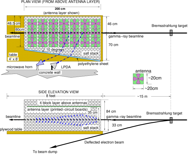
Figure 1: Geometry of salt-block target and receiving antennas in SLAC T460 experiment, from Ref. slac05 .

The particle showers in the salt target were induced by bremsstrahlung gamma-ray photon bunches emanating from an aluminum radiator plate placed in the path of the electron beam. The electron beam itself was deflected to pass below the salt target. The electrons in the beam were accelerated to $\sim$28.5 GeV and the energy of secondary bremsstrahlung photons followed $E^{-1}$ distribution up to $\sim$28.5 GeV. The total energy of photons in each bunch varied with the electron beam intensity and the thickness of the radiator plate.

The salt target was constructed from salt bricks, with a total mass of about 4 metric tons. The detailed description of the target construction can be found in Gorham et al. slac05 . The radio pulses arising from photon induced particle showers were collected by bowtie antenna array embedded in the salt and by a C/X-band horn antenna and an LPDA antenna outside the salt. The bowtie antennas were located in a plane parallel and about 35 cm above the shower axis. The horn and LPDA antennas were placed in the plane of the shower, with LPDA pointing approximately at the expected shower maximum, as indicated in the Fig. 1. The side of salt target facing the external antennas was angled at $10^{\circ}$ in order to allow transmission of Cherenkov radiation which would otherwise have been totally internally reflected. The antennas were read out using digital oscilloscopes, and to improve signal-to-noise ratio (SNR), the recorded waveforms were averaged over many pulses, using an ultra-stable microwave transition-radiation trigger from an upstream location.

The majority of data collected in the experiment was analyzed and published in Ref. slac05 . In order to further test theoretical models of the coherent Cherenkov radiation, this work will concentrate on the analysis of the data collected with the LPDA in two runs, 35 and 109, in which no microwave filters were placed between the LPDA and the oscilloscope, providing the broadest bandwidth data. The total photon bunch energies in these runs were estimated to be 0.48 and 1.1 EeV, respectively, with an uncertainty on the order of 20% due to the beam intensity and the electron bunch energy distribution fluctuations.

The LPDA is an antenna constructed by arranging multiple dipoles in a geometry that provides high signal gain over a large frequency bandwidth kraus . The LPDA antenna used was Electro-Metrics model EM-6952 with nominal bandwidth from 1–18 GHz. The antenna was connected by two pieces of 75–foot heliax cable, Andrew LDF4–50A, and by three pieces of 12–inch semi-rigid Haverhill cable, to a CSA8000 sampling oscilloscope with 20 GHz bandwidth and up to 1000 GSa/s sampling rate.

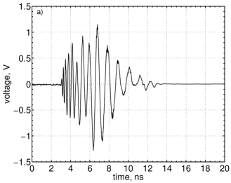
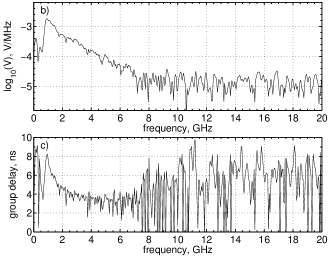
Figure 2: (a) Raw voltage recorded with the LPDA in run 109, and its (b) magnitude and (c) group delay as functions of frequency.

The raw signal recorded in run 109 is shown in Fig. 2, along with its amplitude and group delay, defined as $\tau_{g}(\nu)=(2\pi)^{-1}\frac{d\phi(\nu)}{d\nu}$, where $\phi(\nu)$ is the relative phase of the voltage frequency component, $\phi=\omega t$. It can be seen that the signal is present from $\sim$0.75 GHz (where the LPDA loses sensitivity) to $\sim$7.5 GHz, where the signal strength drops down to the intrinsic oscilloscope noise level. Run 35 signal looks identical except for the increased bandwidth (up to $\sim$11.5 GHz) since no attenuator was used. Fig. 3 shows spectrograms of the recorded signals, with the curvature indicating variations in the delay of voltage frequency components due to the LPDA and the transmission line.

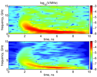
Figure 3: (Color online) Spectrograms of signals recorded in runs 109 and 35 (top and bottom). The color indicates the logarithm of the square root of the signal power per unit frequency.

III System Characterization

In order to reconstruct the electromagnetic radiation pulse incident onto the LPDA (or any other antenna), the signal distorting effects of the antenna and the transmission line have to be corrected. The procedure outlined here is general and applicable to reconstruction of any observation of impulsive radio signals. The antenna equations and the required RF parameters are described in the appendix A.

III.1 Antenna system calibration

The measurement of the LPDA effective height was performed in an anechoic chamber at University of Hawaii by a reciprocal S21 method. Two identical antennas were mounted about 60-in apart facing each other, which ensured they were in each other’s far-field region. For an LPDA, the far-field requirement reduces to $d\geq\lambda/4$, where $d$ is the distance from the point at the LPDA where radiation of wavelength $\lambda$ preferentially couples, i.e., the phase center. The transmitting antenna was stimulated by a 200–mV step impulse generated by an HP 54121A logging head. The received signal was amplified by an Agilent 83017A broadband amplifier and recorded by an HP 54120B digitizing oscilloscope with a 20 GHz bandwidth at 100 GSa/s. The presence of an amplifier introduces a transfer function to the system, so that the expression for the recorded signal $V_{rec}$, combining Eqs. 23 and 24, is

$$V_{rec}(t)=\frac{1}{2\pi rc}H_{amp}(t)\circ h_{N}(t)\circ h_{N}(t)\circ\frac{dV_{src}(t)}{dt},$$ (1)

where $r$ is the antenna separation, $c$ is the speed of light, $V_{src}$ is the voltage stimulating the transmitting antenna, $h_{N}$ is the normalized effective height vector of the antennas, and $H_{amp}$ is the transfer function correction accounting for cables and the amplifier. The scalar product (see Eq. 23) is omitted since the effective height vectors were parallel. The quantity $H_{amp}$ was measured by the same setup, but excluding the antennas from the circuit. Similarly, the heliax cable used in the SLAC measurement was stimulated on one side by a 200–mV step and the resulting pulse was recorded at the other end with the digitizing oscilloscope. The semi-rigid Haverhill cable was unavailable for time-domain transfer function calibration, so only the attenuation was measured as a function of frequency with a network analyzer. Its phase response was ignored, but due to the relatively short length of that cable this omission will have a very small effect on the final result.

III.2 Mathematical operations

In order to calculate the LPDA effective height from calibration measurements, it is conceptually easiest to take a Fourier transform of Eq. 1 and re-arrange it so that

$$\tilde{h}_{N}(\nu)=\sqrt{\frac{rc}{i\nu}\frac{\tilde{V}_{rec}(\nu)}{\tilde{H}_{amp}(\nu)\tilde{V}_{src}(\nu)}},$$ (2)

where $\tilde{f}(\nu)=\int f(t)e^{2\pi i\nu t}dt$. Also, from Eq. 24, $\tilde{H}_{amp}(\nu)=\tilde{V}_{out}(\nu)/\tilde{V}_{in}(\nu)$. The same expression is also applied to calculate the transfer function of heliax cable. All operations, including the square root, are performed using complex quantities. Special care should be taken when taking a complex square root in order to properly account for phase wrapping.

While straightforward, this frequency-domain based approach will give poor time-domain results if the frequency bandwidth of a measured signal is substantially narrower than the Nyquist limit of the sampling oscilloscope. The time-domain result of a complex division operation in the frequency-domain will be dominated by frequency components where the signal is absent, i.e., where a division of two small noise values can produce an arbitrarily large artificial result. Digital signal processing tools can be applied to filter out such artificial “out-of-band” noise, but they will in all cases produce an unacceptable level of signal distortion. In order to circumvent this issue, a time-domain deconvolution algorithm with noise reduction can be applied in place of every complex division operation. In this work, the Wiener algorithm was chosen wiener , and the level of the noise-to-signal power ratio required by the algorithm was chosen such to maximize out-of-band noise rejection while preserving the fidelity of the in-band signal (see Fig. 5b).

The resulting time-domain response of the LPDA-cable system as used in the experiment can be expressed as $\bm{h}_{sys}(t)=H_{cable}(t)\circ\bm{h}_{N,LPDA}(t)$ and is shown in Fig. 4.

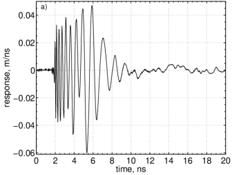
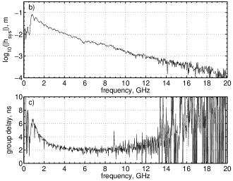
Figure 4: (a) Time-domain response, and (b) attenuation and (c) group delay as functions of frequency for the LPDA-cable system used in the measurements. The phase coherence of calibration pulses extends to $\sim$13 GHz, which exceeds the usable bandwidth of experimental data. The feature visible in group delay plot at $\sim$8.9 GHz is due to reflections at the amplifier input and it was not possible to calibrate it out. However, it does not create any appreciable effect in the final result.

IV Analysis

The voltages recorded in the experiment can be expressed as (see Eqs. 19–21)

$$V_{rec}(t)=\sqrt{\frac{Z_{L}}{Z_{0}}}\bm{h}_{sys}(t)\star\bm{E}_{ant}(t),$$ (3)

where $\bm{E}_{ant}$ is the electric field at the antenna due to the particle shower. During the measurements, the LPDA was aligned such that the polarization of electric field was parallel to the effective height vector, so that the spatial scalar product drops out of the equation. Thus, in the frequency domain, the electric field at the antenna is given by

$$\tilde{E}_{ant}(\nu)=\sqrt{\frac{Z_{0}}{Z_{L}}}\frac{\tilde{V}_{rec}(\nu)}{\tilde{h}_{sys}(\nu)},$$ (4)

with $Z_{L}=50\Omega$. The resulting electric field is shown in Fig. 5.

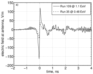
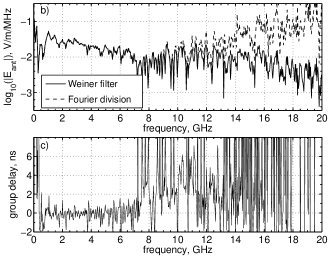
Figure 5: The electric fields at the antenna in two runs (a), and the magnitude (b) and the group delay (c) as functions of frequency (for run 109 only). In (b), the dashed line shows the magnitude obtained by straight frequency-domain division. The signal is dominated by artificial noise at frequencies outside of the signal bandwidth (0.75–7.5 GHz). It is clear that the use of the Wiener deconvolution algorithm is justified since it preserves the signal “in-band” while suppressing the “out-of-band” noise.

Before the measured electric fields can be compared with the theoretical expectation, several corrections have to be applied. The theory was derived for a pulse detected at a very large distance from a shower initiated by a single particle, i.e., where the shower can be considered a point source emitter and the radiation emitted is coherent over the full length of the shower. Additionally, the detection is also assumed to be in the same medium as the emission. In the experimental setup this is not the case. Aside from accounting for the electric field divergence as it crosses from salt to air, the portion of the particle shower generating a coherent pulse at the antenna scales with the frequency of observation. Finally, the number of particles at the shower maximum, $N_{max}$, due to the superposition of many low-GeV electromagnetic showers will be larger than $N_{max}$ due to a shower initiated by a single particle of the equivalent energy. Since the intensity of the radiation emitted is proportional to $N_{max}$, this difference has to be taken into account.

IV.1 Coherence zone correction

The standard radiation coherence requirement is that phases of rays emerging from two ends of a coherence zone do not differ by more than one cycle ($2\pi$) at any given frequency. The geometry of this requirement in the present case is sketched in Fig. 6a.

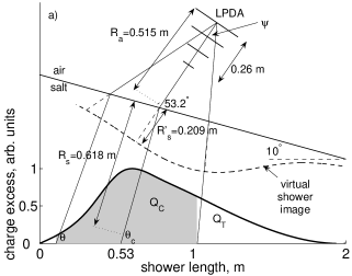
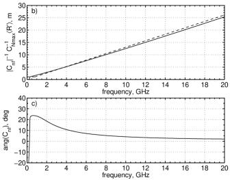
Figure 6: a) A sketch of the experimental geometry, including the coherence zone (shaded) and the charge excess distribution as measured by the embedded bowtie antennas slac05 . The dashed line, labeled virtual shower image, indicates the non-trivial path along which the shower appears to develop due to the salt/air interface, as seen by an observer located at the LPDA feedpoint. b) The correction factor magnitude and c) phase as functions of frequency (see text). The dashed line in b) is the ad-hoc correction factor used in Ref. slac05 .

Thus, the zone of coherence about a point on the shower axis that the antenna is pointed at ($z_{C}$), can be defined for $z$’s satisfying the condition

$$\Delta\phi(z;\nu)=\left|R^{\prime\prime}_{s}(z;\nu)-R^{\prime\prime}_{s}(z_{C};\nu)+\frac{z-z_{C}}{n}\right|\frac{2\pi}{\lambda}\leq\pi,$$ (5)

where $z_{C}=0.53$ m, $n=2.44$ is the index of refraction of salt, radiation wavelength $\lambda=\frac{c}{n\nu}$, and $R^{\prime\prime}_{s}(z;\nu)$ is the apparent distance from a point on the shower axis to the phase center of the antenna for the given frequency as if the entire path was in salt, i.e., the number of actual phase cycles, $N$, is preserved and $R^{\prime\prime}_{s}=N\lambda$. Eq. 5 is simply a restatement of the difference in phase factors of an electric field due to a moving charge without making a Fraunhofer zone approximation jackson . For the phase center of the LPDA, a simple model is assumed where the phase center moves linearly along the antenna axis, such that the 1–GHz phase center is at the feed-point and the 20–GHz phase center is at the tip of the antenna, about 26 cm from the feed-point. While not exact, this model is sufficiently accurate not to contribute strongly to systematic errors. As an example, the coherence zones at 1 GHz and 5 GHz were found to be $z=[0,1.05]$ m and $z=[0.45,0.77]$ m, respectively.

With the coherence zone defined, a correction to the electric field at the antenna with respect to the electric field at infinity can be made. From Refs. zhs ; am ; forte , the electric field due to coherent Cherenkov radiation at a given angle is proportional to the integral over the current distribution in the particle shower, $J(z)=c\;q(z)$, and to geometric factors relative to emission and observation points,

$$E(\nu,\theta)\propto\int e^{ik(R\cos{\theta}+z/n)}q(z)dz,$$ (6)

where $k=\frac{2\pi}{\lambda}$, $R$ is the distance from an emission point to the observation point, $\theta$ is the angle of emission, and the integral is taken over the full length of the shower. Taking into consideration the geometry of the experiment, a near-field correction factor relative to observation made at infinity along the Cherenkov angle can be defined as

$$C_{nf}(\nu)=\frac{\int_{z_{1}(\nu)}^{z_{2}(\nu)}e^{i\Delta\phi}q(z)\;T\;G\;\frac{\sin{\theta}}{\sin{\theta_{C}}}e^{-\frac{1}{2}\left(\frac{\theta-\theta_{C}}{\Delta\theta(\nu)}\right)^{2}}dz}{\int_{0}^{2}q(z)dz},$$ (7)

where $[z_{1}(\nu),z_{2}(\nu)]$ defines the coherence zone at a given frequency, $T\equiv T(z;\nu)$ is the transmission coefficient through the salt/polyethylene/air interface, $G\equiv G(z;\nu)$ is the relative gain of the LPDA away from the antenna boresight, and $\theta\equiv\theta(z;\nu)$. The last two terms of the integrand in the numerator account for the drop in the electric field magnitude away from Cherenkov angle, with $\Delta\theta=4.65^{\circ}\left[\frac{1\;\text{GHz}}{\nu}\right]$ am .

The transmission coefficient is given by the Fresnel equation for the E-field parallel to the plane of incidence jackson ,

$$T=\frac{E^{\prime}_{||}}{E_{||}}=\frac{2n\cos{i}}{n\cos{r}+n^{\prime}\cos{i}},$$

where $i$ and $r$ are incident and refracted angles related by Snell’s law, and $n$ and $n^{\prime}$ are indices of refraction in the two media. In calculating the transmission coefficient, the presence of the 2.5 cm thick polyethylene sheet ($n_{poly}=2.25$) is ignored at frequencies below 2.5 GHz (half-wavelength thickness) and its effect is gradually turned on to full strength above 10 GHz (two-wavelength thickness). The relative gain of the LPDA as a function of frequency was not measured, but was modeled based on the manufacturer’s specification of $70^{\circ}$ average beam-width in the antenna E-plane and the standard LPDA expectation of first null at twice the beam-width, to be $G(\psi)\approx\sqrt{\cos({\frac{90^{\circ}}{70^{\circ}}\psi})}$, with $\psi$ being the angle relative to the antenna boresight.

When presenting the preliminary results of this analysis in Ref. slac05 , it has been argued that the coherence zone extends over the full shower at frequencies below 800 MHz, and that at higher frequencies the near-field correction is proportional to $\nu$. In Fig. 6b, it can be seen that this simplification was reasonable as it produced an adequate near-field correction.

IV.2 Field divergence at the salt/air interface

The $1/R$ attenuation in the electric field has to be modified for the field divergence at the salt/air interface. The field divergence factor for a spherical wave incident on a planar interface can be calculated by considering an area element $dA$ of the surface,

$$dA=\frac{R_{s}^{2}d\Omega}{\cos{i}}=\frac{{R^{\prime}_{s}}^{2}d\Omega^{\prime}}{\cos{r}},$$ (8)

where $d\Omega$ is the solid angle element subtending $dA$ as seen from the emission point, $d\Omega^{\prime}$ is the solid angle element subtending field lines exiting through $dA$, $R_{s}$ is the distance from the emission point to the salt/air interface, $R^{\prime}_{s}$ is the distance from the virtual emission point as seen from the outside, and $i$ and $r$ are incident and refracted angles as determined by Snell’s law. The field divergence factor is given by the ratio of true and virtual distances forte ,

$$\frac{R_{s}}{R^{\prime}_{s}}=\frac{n\cos{i}}{\cos{r}}.$$ (9)

The effective distance from an emission point to the LPDA is then given by,

$$R^{\prime}(z;\nu)=R_{a}(z;\nu)\frac{n\cos{i(z;\nu)}}{\cos{r(z;\nu)}}+R_{s}(z;\nu),$$ (10)

where $R_{a}$ is the distance from the salt/air interface to the LPDA. The reader can easily convince oneself that the presence of the polyethylene sheet cancels out when considering the field divergence in the experimental setup. The mean LPDA to shower distance at any given frequency is then

$$\langle R^{\prime}(\nu)\rangle=\frac{\int_{z_{1}}^{z_{2}}R^{\prime}(z;\nu)dz}{\int_{z_{1}}^{z_{2}}dz}.$$ (11)

IV.3 $N_{max}$ correction

The energy of photons initiating particle showers in the SLAC experiment was from $\sim$1–28500 MeV, with a $1/E$ bremsstrahlung distribution. The theoretical work on coherent Cherenkov radiation is based on simulations of electromagnetic showers initiated by primaries with energies of 1 TeV and above zhs ; am . While $N_{max}$, the number of particles at the shower maximum, scales nearly linearly with the energy of the primary at $E_{p}\gtrsim 10$ TeV, this is not the case for the lower energy primaries. The EGS4 simulation shows that a bremsstrahlung photon bunch with the total energy of 20.7 TeV hitting the salt target will produce $N_{max}\approx 55000$. However, the 20.7–TeV electron primary, interacting in the salt, gives rise to a shower whose peak is deeper and broader, and hence has only $\sim$19500 particles at the shower maximum gaisser .Thus, $C_{Nmax}=2.82$ can be defined as a correction factor to be used when comparing to theoretical results.

Putting all these corrections together, the measured electric field can be compared to the one which would have been expected from an equivalent shower observed in salt in the far-field region at Cherenkov angle,

$$R|E(\nu,\theta_{C})|=\frac{\langle R^{\prime}(\nu)\rangle E_{ant}(\nu)}{C_{nf}C_{Nmax}}.$$ (12)

The corrections will be applied only in the frequency range where the coherent signals are present in order not to amplify the thermal noise background.

V Discussion

The far-field corrected pulses, and their magnitudes and phases, are shown in Fig. 7.

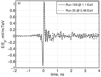
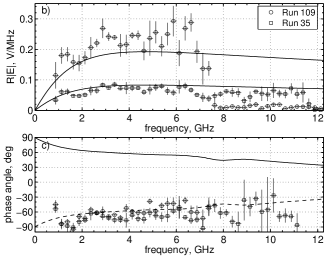
Figure 7: (a) Electric field due to Askaryan pulses from two runs renormalized to 1 TeV primary energy; (b) electric field magnitudes as functions of frequency compared to the expectations; (c) electric field phases as functions of frequency, calculated relative to the zero-crossing point, compared to the expectation for an Askaryan pulse in salt (solid line) zhs . The dashed line places the theoretical phase expectation in the fourth quadrant, see text.

The magnitude and phase information have been binned in 250 MHz bins for clarity, and error bars indicate the RMS variation within each bin. The expectation for the magnitude of the electric field is given by am ; slac05

$$R|E|=A_{0}f_{d}\left[\frac{E_{p}}{1\text{TeV}}\right]\left[\frac{\nu}{\nu_{0}}\right]\left[\frac{1}{1+(\nu/\nu_{1})^{1.44}}\right],$$ (13)

where $A_{0}=2.53\times 10^{-7}$ V/MHz, $f_{d}=0.52$, $\nu_{0}=1.15$ GHz, and $\nu_{1}=2.86$ GHz. The standard Fourier transform of the measured electric field was multiplied by a factor of 2 in order to agree with the definition of Eq. 8 in Ref. zhs adopted in Refs. am ; slac05 .

The only published electric field phase expectation has been calculated for an Askaryan pulse in ice zhs , but there is no reason to expect any significant deviation in the case of salt. However, there are two ambiguities that have to be resolved before a meaningful comparison of measured and expected phases can be made. The first is the actual quadrant of the phase. In the early theoretical calculations, the signs of the real and imaginary parts of the Fourier transform of the electric field were not kept shahid , and thus the complete phase information was unavailable. Newer calculations indicate that the phase is expected to lie in the fourth quadrant shahid , and the dashed line in Fig. 7c indicates such a choice, which will be considered as correct in the remainder of this discussion. The second ambiguity is in the choice of the reference time about which to calculate the phase angle. No convention has been put forward, but one could expect that a natural choice would be the time of arrival of radiation from the shower maximum in the direction of the Cherenkov angle. Unfortunately, in the present experiment the relative oscilloscope trigger time with respect to the beam pulse was not recorded. The best guess would be to take the zero-crossing time in the middle of the pulse as was done in Fig. 7c. A choice of a different reference time introduces an artificial phase slew, which can obscure the real physical features related to the phase, like the current distribution in the shower.

A few features of the recorded pulses should be noted. The signals were recorded from 0.75–11.5 GHz in run 35 and 0.75–7.5 GHz in run 109. This is indicated by the loss of both the phase coherence and the SNR above these frequencies due to attenuation in the antenna system, which increases with the frequency. As noted before, a 20 dB attenuator was present in run 109, causing the additional bandwidth loss. A clear way to present an impulsive, coherent, broadband signal expected from coherent Cherenkov radiation is with a spectrogram (Fig. 8). The pulse arrival is seen at zero time, with some low level reflections trickling in at the later times.

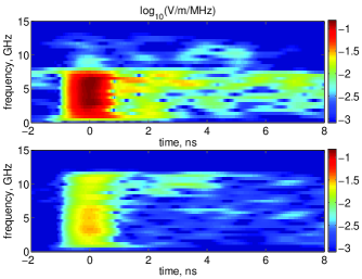
Figure 8: (Color online) Spectrograms of electric fields due to Askaryan pulse recorded in runs 109 and 35 (top and bottom), where the color indicates the logarithm of the square root of electric field power per unit frequency. The reconstructed impulses are coherent and unresolved at all frequencies.

The effect of deconvolving system response, Eq. 4, and applying corrections, Eq. 12, can be seen by comparing to Fig. 3.

Figure 9: Distributions of bin-by-bin differences in expected and measured magnitudes and phases of electric fields, over signal bandwidths noted in the text. The magnitudes have been renormalized to 1 TeV shower energy. The fits are Gaussian.

Although deviations from theoretical expectations in Figs. 7b and 7c appear to be systematic since they are correlated between the runs, they are actually due to noise in the calibration data. This can be clearly seen in Fig. 9 which histograms bin-by-bin differences between expectation and measurements over the signal bandwidth. The full frequency resolution of 50 MHz per bin was used. The deviations from expectation are Gaussian in nature, implying random noise. The offsets in the means of difference in magnitude can be attributed to systematic errors in the energy calibration of the runs, while the offset in the means of difference in phase, can be attributed to the choice of phase reference time. Changing the reference time by 8(1) ps for run 35(109) shifts the mean to 0^∘ while preserving the width of the distribution. Considering that the digitization time resolution is 10(20) ps, this indicates a shift of less than one timing bin in both cases. Also, one could chose to use the predicted intensity of Cherenkov radiation in order to calibrate the total energy of showers in two runs. Minimizing the mean of the difference in magnitude, the shower energies are found to be 0.38 EeV and 1.36 EeV, respectively. Combining the distributions from two runs, the fitted deviations are $\Delta(R|E|/E_{p})=-0.005\pm 0.039\text{(stat)}\pm 0.045\text{(sys)}\;\mu\text{V/MHz/TeV}$ and $\Delta\phi=-9^{\circ}\pm 17^{\circ}\text{(stat)}\pm 22^{\circ}\text{(sys)}$. Thus, it can be concluded that the theoretical expectations for magnitude and phase of the electric field zhs ; slac05 due to coherent Cherenkov radiation in salt in the frequency range from 0.75–11.5 GHz have been confirmed within experimental uncertainty.

In this work, the procedure for the time-domain based analysis of antenna measurements and calibrations has been described and successfully applied to measurements of coherent Cherenkov radiation made at the FFTB facility at SLAC. The time-domain signal analysis preserves both magnitude and phase information of the original pulse, allowing for more accurate validation of theoretical models. The most precise validation of electric field intensity and the first validation of electric field phase of the theoretical model has been performed.

*

Appendix A Antenna equations

The voltage at the antenna port delivered to the transmission line of characteristic impedance $Z_{L}$ by the antenna with impedance $Z_{a,Rx}$ can be defined as shliv ; baum1 ,

$$V_{L}(t)=\tau_{Rx}\;\bm{h}_{e,Rx}(t)\star\bm{E}(t),$$ (14)

with

$$\tau_{Rx}=\frac{2Z_{L}}{Z_{a,Rx}+Z_{L}},$$

where $\star$ is the operator combining temporal convolution and spatial scalar product, $\bm{E}$ is the incident electric field and $\bm{h}_{e,Rx}$ is the time-dependent effective height of the antenna for reception. The time-dependent effective height is the time-domain representation of the antenna complex impedance, and is equivalent to the antenna response to a delta-like impulse.

At this point it is useful to also write down the equation for the electric field at some distance from the antenna transmitting an impulsive signal driven through the transmission line of characteristic impedance $Z_{L}$ by a voltage source $V_{src}$,

$$\bm{E}(t)=\frac{1}{4\pi rc}f_{Tx}\;\tau_{Tx}\;\bm{h}_{e,Tx}(t)\circ V_{src}(t),\\$$ (15)

with

$$f_{Tx} = \frac{Z_{0}}{Z_{a,Tx}},$$

$$\tau_{Tx} = \frac{2Z_{a,Tx}}{Z_{L}+Z_{a,Tx}},$$

where $\circ$ is the convolution operator, $Z_{a,Tx}$ is the transmitting antenna impedance, $Z_{0}$ is the impedance of free space ($377\Omega$), and $\bm{h}_{e,Tx}$ is the time-dependent effective height of the antenna for transmission. The voltage $V_{src}$ as used here is the voltage that would have been read by an oscilloscope if it were connected to the voltage source instead of an antenna and matched to the transmission line. Eq. 15 can be rewritten using the relation between transmission and reception effective heights of an antenna derived from self-reciprocity arguments shliv ,

$$\bm{h}_{e,Tx}(t)=2\partial_{t}\bm{h}_{e,Rx}(t).$$ (16)

Substituting Eq. 16 into Eq. 15 and noting that time derivation and convolution commute, the transmission equation can be written as,

$$\bm{E}(t)=\frac{1}{2\pi rc}f_{Tx}\;\tau_{Tx}\;\bm{h}_{e,Rx}(t)\circ\frac{dV_{src}(t)}{dt}.$$ (17)

Both antenna transmission and reception are now defined using the same effective height quantity.

The form of the preceding equations assumes that both the antenna and the transmission line have purely resistive impedance. The equations can be simplified and the complex antenna impedance can be reintroduced by absorbing the voltage transmission coefficient into the definition of effective height and renormalizing voltages and electric fields as suggested by Farr and Baum farr . Using the following variable substitutions,

$$\bm{h}_{N}(t) = \frac{2\sqrt{Z_{0}Z_{L}}}{Z_{a}+Z_{L}}\bm{h}_{e,Rx}(t),$$ (18)

$$V_{N}(t) = \frac{V(t)}{\sqrt{Z_{L}}},$$ (19)

$$\bm{E}_{N}(t) = \frac{\bm{E}(t)}{\sqrt{Z_{0}}},$$ (20)

where $Z_{a}$, $V$, and $\bm{E}$ stand for both transmission and reception cases, the antenna equations become

$$V_{N,L}(t) = \bm{h}_{N}(t)\star\bm{E}_{N}(t),$$ (21)

$$\bm{E}_{N}(t) = \frac{1}{2\pi rc}\bm{h}_{N}(t)\circ\frac{dV_{N,src}(t)}{dt}.$$ (22)

Finally, if two identical antennas separated by distance $r$ are used to transmit and receive, and transmission lines with the same impedance are used at both ends, the voltage observed on the port of the receiving antenna is given by

$$V_{L}(t)=\frac{1}{2\pi rc}\bm{h}_{N}(t)\star\bm{h}_{N}(t)\circ\frac{dV_{src}(t)}{dt}.$$ (23)

The transmission line complex impedance can be handled by introducing a transfer function correction, $H$, which accounts for phase and amplitude distortions of a broadband signal traveling through the transmission line. In the time-domain based description, this correction is expressed as

$$V_{out}(t)=H(t)\circ V_{in}(t).$$ (24)

All of the antenna equations above need to include transmission line transfer function corrections at appropriate places, depending on the actual system setup. One should keep in mind that convolution operators commute, so that contributions from several transmission line segments (even ones at the opposite transmission/reception ends of the system) can be combined into a single transfer function.

- (1) G. A. Askaryan, JETP 14, 441 (1962); JETP 21, 658 (1965).
- (2) E. Zas, F. Halzen, and T. Stanev, Phys. Rev. D45, 362 (1992).
- (3) J. Alvarez-Muñiz, R. A. Vázquez, and E. Zas, Phys. Rev. D62 063001 (2000).
- (4) S. Razzaque et al., Phys. Rev. D65, 103002 (2002); errata Phys. Rev. D69, 047101 (2004).
- (5) D. Saltzberg et al., Phys. Rev. Lett. 86, 2802 (2001).
- (6) P. Gorham et al., Phys. Rev. D72, 023002 (2005).
- (7) N. G. Lehtinen, P. W. Gorham, A. R. Jacobson, and R. A. Roussel-Dupre, Phys. Rev. D69 013008 (2004).
- (8) I. Kravchenko et al., Phys. Rev. D73 082002 (2006).
- (9) S. W. Barwick et al., Phys. Rev. Lett. 96, 171101 (2006).
- (10) P. Miočinović et al., astro-ph/0503304; A. Silvestri et al., astro-ph/0411007
- (11) R. D. Dagkesamanskii and I. M. Zheleznyk, JETP 50, 233 (1989).
- (12) P. W. Gorham et al., Phys. Rev. Lett. 93, 041101 (2004).
- (13) J. D. Kraus, Antennas, 2 ed. (McGraw-Hill, New York, 1988).
- (14) N. Wiener, Extrapolation, Interpolation, and Smoothing of Stationary Time Series, (Wiley, New York, 1949).
- (15) J. D. Jackson, Classical Electrodynamics, 2 ed. (John Wiley & Sons, New York, 1975).
- (16) T. K. Gaisser, Cosmic Rays and Particle Physics, (Cambridge University Press, Cambridge, 1990).
- (17) S. Hussain, private communication
- (18) A. Shlivinski, E. Heyman, and R. Kastner, IEEE T. Antenn. Propag. 45 1140 (1997).
- (19) C. E. Baum, IEEE T. Electromagn. C. 44, 18 (2002).
- (20) E. G. Farr and C. E. Baum, Sensor and Simulation Note 426 (1998); http://www-e.uni-magdeburg.de/notes