Theoretical and experimental status of magnetic monopoles

Abstract

The Tevatron has inspired new interest in the subject of magnetic monopoles. First there was the 1998 D0 limit on the virtual production of monopoles, based on the theory of Ginzburg and collaborators. In 2000 and 2004 results from an experiment (Fermilab E882) searching for real magnetically charged particles bound to elements from the CDF and D0 detectors were reported. The strongest direct experimental limits, from the CDF collaboration, have been reported in 2005. Less strong, but complementary, limits from the H1 collaboration at HERA were reported in the same year. Interpretation of these experiments also require new developments in theory. Earlier experimental and observational constraints on point-like (Dirac) and non-Abelian monopoles were given from the 1970s through the 1990s, with occasional short-lived positive evidence for such exotic particles reported. The status of the experimental limits on monopole masses will be reported, as well as the limitation of the theory of magnetic charge at present.

1 Introduction

The origin of the concept of magnetic charge, if not the name, goes back to antiquity. Certain stones in Magnesia, in Anatolia (Asia Minor), were found to exhibit an attractive force on iron particles, and thus was discovered magnetism. (Actually there is an ancient confusion about the origin of the name, for it may refer to Magnesia, a prefecture in Thessaly, Greece, from whence came the settlers (“Magnets”) of the city (or the ruins of another city) which is now in Turkey. For a recent discussion on the etymology see [1].) Electricity likewise was apparent to the ancients, but without any evident connection to magnetism. Franklin eventually posited that there were two kinds of electricity, positive and negative poles or charge; there were likewise two types of magnetism, north and south poles, but experience showed that those poles were necessarily always associated in pairs. Cutting a magnet, a dipole, in two did not isolate a single pole, but resulted in two dipoles with parallel orientation; the north and south poles so created were bound to the opposite poles already existing [2]. This eventually was formalized in Ampère’s hypothesis (1820): Magnetism has its source in the motion of electric charge. That is, there are no intrinsic magnetic poles, but rather magnetic dipoles are created by circulating electrical currents, macroscopically or at the atomic level.

Evidently, the latter realization built upon the emerging recognition of the connection between electricity and magnetism. Some notable landmarks along the way were Oersted’s discovery (1819) that an electrical current produced magnetic forces in its vicinity; Faraday’s visualization of lines of force as a physical picture of electric and magnetic fields; his discovery that a changing magnetic field produces a electric field (Faraday’s law of magnetic induction, 1831); and Maxwell’s crowning achievement in recognizing that a changing electric field must produce a magnetic field, which permitted him to write his equations describing electromagnetism (1873). The latter accomplishment, built on the work of many others, was the most important development in the 19th Century. It is most remarkable that Maxwell’s equations, written down in a less than succinct form in 1873, have withstood the revolutions of the 20th Century, relativity and quantum mechanics, and they still hold forth unchanged as the governing field equations of quantum electrodynamics, by far the most successful physical theory ever discovered.

The symmetry of Maxwell’s equations was spoiled, however, by the absence of magnetic charge, and it was obvious to many, including Poincaré [3] and Thomson [4, 5], the discoverer of the electron, that the concept of magnetic charge had utility, and its introduction into the theory results in significant simplifications. (Faraday [6] had already demonstrated the heuristic value of magnetic charge.) But at that time, the consensus was clearly that magnetic charge had no independent reality, and its introduction into the theory was for computational convenience only [7], although Pierre Curie [8] did suggest that free magnetic poles might exist. It was only well after the birth of quantum mechanics that a serious proposal was made by Dirac [9] that particles carrying magnetic charge, or magnetic monopoles, should exist. This was based on his observation that the phase unobservability in quantum mechanics permits singularities manifested as sources of magnetic fields, just as point electric monopoles are sources of electric fields. This was only possible if the product of electric and magnetic charges was quantized. This prediction was an example of what Gell-Mann would later call the “totalitarian principle” – that anything which is not forbidden is compulsory [10]. Dirac eventually became disillusioned with the lack of experimental evidence for magnetic charge, but Schwinger, who became enamored of the subject around 1965, never gave up hope. This, in spite of his failure to construct a computationally useful field theory of magnetically charged monopoles, or more generally particles carrying both electric and magnetic charge, which he dubbed dyons (for his musing on the naming of such hypothetical particles, see [11]). Schwinger’s failure to construct a manifestly consistent theory caused many, including Sidney Coleman, to suspect that magnetic charge could not exist. The subject of magnetic charge really took off with the discovery of extended classical monopole solutions of non-Abelian gauge theories by Wu and Yang, ’t Hooft, Polyakov, Nambu, and others [12, 13, 14, 15, 16, 17]. With the advent of grand unified theories, this implied that monopoles should have been produced in the early universe, and therefore should be present in cosmic rays. (The history of magnetic monopoles up to 1990 is succinctly summarized with extensive references in the Resource Letter of Goldhaber and Trower [18].)

So starting in the late 1960s there was a burst of activity both in trying to develop the theory of magnetically charged particles and in attempting to find their signature either in the laboratory or in the cosmos. As we will detail, the former development was only partially successful, while no evidence at all of magnetic monopoles has survived. Nevertheless, the last few years, with many years of running of the Tevatron, and on the eve of the opening of the LHC, have witnessed new interest in the subject, and new limits on monopole masses have emerged. However, the mass ranges where monopoles might most likely be found are yet well beyond the reach of earth-bound laboratories, while cosmological limits depend on monopole fluxes, which are subject to large uncertainties. It is the purpose of this review to summarize the state of knowledge at the present moment on the subject of magnetic charge, with the hope of focusing attention on the unsettled issues with the aim of laying the groundwork for the eventual discovery of this exciting new state of matter.

A word about my own interest in this subject. I was a student of Julian Schwinger, and co-authored an important paper on the subject with him in the 1970s [19]. Many years later my colleague in Oklahoma, George Kalbfleisch, asked me to join him in a new experiment to set limits on monopole masses based on Fermilab experiments [20, 21]. His interest grew out of that of his mentor Luis Alvarez, who had set one of the best earlier limits on low-mass monopoles [22, 23, 24, 25, 26]. Thus, I believe I possess the bona fides to present this review.

Finally, I offer a guide to the reading of this review. Since the issues are technical, encompassing both theory and experiment, not all parts of this review will be equally interesting or relevant to all readers. I have organized the review so that the main material is contained in sections and subsections, while the third level, subsubsections, contains material which is more technical, and may be omitted without loss of continuity at a first reading. Thus in section 3, sections 3.1.1–3.1.6 constitute a detailed proof of the quantization condition, while section 3.2 describes the quantum mechanical cross section.

In this review we use Gaussian units, so, for example, the fine-structure constant is $\alpha=e^{2}/\hbar c$. We will usually, particularly in field theoretic contexts, choose natural units where $\hbar=c=1$.

2 Classical theory

2.1 Dual symmetry

The most obvious virtue of introducing magnetic charge is the symmetry thereby imparted to Maxwell’s equations in vacuum,

$$\boldsymbol{\nabla}\cdot{\bf E}=4\pi\rho_{e},\qquad\boldsymbol{\nabla}\cdot{\bf B}=4\pi\rho_{m},$$

$$\boldsymbol{\nabla}\times{\bf B}={1\over c}{\partial\over\partial t}{\bf E}+{4\pi\over c}{\bf j}_{e},\qquad-\boldsymbol{\nabla}\times{\bf E}={1\over c}{\partial\over\partial t}{\bf B}+{4\pi\over c}{\bf j}_{m}.$$ (2.1)

Here $\rho_{e}$, ${\bf j}_{e}$ are the electric charge and current densities, and $\rho_{m}$, ${\bf j}_{m}$ are the magnetic charge and current densities, respectively. These equations are invariant under a global duality transformation. If $\cal E$ denotes any electric quantity, such as $\bf E$, $\rho_{e}$, or ${\bf j}_{e}$, while $\cal M$ denotes any magnetic quantity, such as $\bf B$, $\rho_{m}$, or ${\bf j}_{m}$, the dual Maxwell equations are invariant under

$${\cal E}\to{\cal M},\quad{\cal M}\to-{\cal E},$$ (2.2a)

or more generally

$${\cal E}\to{\cal E}\cos\theta+{\cal M}\sin\theta,\qquad{\cal M}\to{\cal M}\cos\theta-{\cal E}\sin\theta,$$ (2.2b)

where $\theta$ is a constant.

Exploitation of this dual symmetry is useful in practical calculations, even if there is no such thing as magnetic charge. For example, its appearance may be used to facilitate an elementary derivation of the laws of energy and momentum conservation in classical electrodynamics [27]. A more elaborate example is the use of fictitious magnetic currents in calculate diffraction from apertures [28]. (See also [29].)

2.2 Angular momentum

J. J. Thomson observed in 1904 [4, 5, 30, 31] the remarkable fact that a static system of an electric ($e$) and a magnetic ($g$) charge separated by a distance $\bf R$ possesses an angular momentum, see figure 1.

Figure 1: Static configuration of an electric change and a magnetic monopole.

The angular momentum is obtained by integrating the moment of the momentum density of the static fields:

$${\bf J}=\int(\rmd{\bf r})\,{\bf r\times G}=\int(\rmd{\bf r})\,{\bf r}\times\frac{{\bf E\times B}}{4\pi c}$$

$$=\frac{1}{4\pi c}\int(\rmd{\bf r})\,{\bf r}\times\left[\frac{e{\bf r}}{r^{3}}\times\frac{g({\bf r-R})}{({\bf r-R})^{3}}\right]=\frac{eg}{c}{\bf\hat{R}},$$ (2.2c)

which follows from symmetry (the integral can only supply a numerical factor, which turns out to be $4\pi$ [27]). The quantization of charge follows by applying semiclassical quantization of angular momentum:

$${\bf J\cdot\hat{R}}=\frac{eg}{c}=n\frac{\hbar}{2},\qquad n=0,\,\pm 1,\,\pm 2,\,\dots,$$ (2.2da)

or

$$eg=m^{\prime}\hbar c,\qquad m^{\prime}=\frac{n}{2}.$$ (2.2db)

(Here, and in the following, we use $m^{\prime}$ to designate this “magnetic quantum number.” The prime will serve to distinguish this quantity from an orbital angular momentum quantum number, or even from a particle mass.)

2.3 Classical scattering

Actually, earlier in 1896, Poincaré [3] investigated the motion of an electron in the presence of a magnetic pole. This was inspired by a slightly earlier report of anomalous motion of cathode rays in the presence of a magnetized needle [32]. Let us generalize the analysis to two dyons (a term coined by Schwinger in 1969 [11]) with charges $e_{1}$, $g_{1}$, and $e_{2}$, $g_{2}$, respectively. There are two charge combinations

$$q=e_{1}e_{2}+g_{1}g_{2},\qquad\kappa=-{e_{1}g_{2}-e_{2}g_{1}\over c}.$$ (2.2de)

Then the classical equation of relative motion is ($\mu$ is the reduced mass and $\bf v$ is the relative velocity)

$$\mu{\rmd^{2}\over\rmd t^{2}}{\bf r}=q{{\bf r}\over r^{3}}-\kappa{\bf v}\times{{\bf r}\over r^{3}}.$$ (2.2df)

The constants of the motion are the energy and the angular momentum,

$$E={1\over 2}\mu v^{2}+{q\over r},\qquad{\bf J}={\bf r\times\mu v}+\kappa{\bf\hat{r}}.$$ (2.2dg)

Note that Thomson’s angular momentum (2.2c) is prefigured here.

Because $\bf J\cdot\hat{r}=\kappa$, the motion is confined to a cone, as shown in figure 2.

Figure 2: The relative motion of two dyons is confined to the surface of a cone about the direction of the angular momentum.

Here the angle of the cone is given by

$$\cot{\chi\over 2} = {l\over|\kappa|},\qquad l=\mu v_{0}b,$$ (2.2dh)

where $v_{0}$ is the relative speed at infinity, and $b$ is the impact parameter. The scattering angle $\theta$ is given by

$$\cos\frac{\theta}{2}=\cos\frac{\chi}{2}\left|\sin\left(\frac{\xi/2}{\cos\chi/2}\right)\right|,$$ (2.2dia)

where

$$\frac{\xi}{2}=\left\{\begin{array}[]{cc}\arctan\left(\frac{|\kappa|v_{0}}{q}\cot\frac{\chi}{2}\right),&q>0,\\ \pi-\arctan\left(\frac{|\kappa|v_{0}}{|q|}\cot\frac{\chi}{2}\right),&q<0.\end{array}\right.$$ (2.2dib)

When $q=0$ (monopole-electron scattering), $\xi=\pi$. The impact parameter $b(\theta)$ is a multiple-valued function of $\theta$, as illustrated in figure 3.

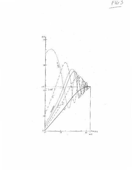
Figure 3: Scattering angle $\theta$ as a function of the impact parameter variable $\chi$. Here $k\pi=|\kappa|v_{0}/q$.

The differential cross section is therefore

$$\frac{\rmd\sigma}{\rmd\Omega}=\left|\frac{b\,\rmd b}{\rmd(\cos\theta)}\right|=\left(\frac{\kappa}{\mu v_{0}}\right)^{2}\underbrace{\sum_{\chi}\frac{1}{4\sin^{4}\frac{\chi}{2}}\left|\frac{\sin\chi\,\rmd\chi}{\sin\theta\,\rmd\theta}\right|}_{g(\theta)}.$$ (2.2dij)

Representative results are given in [19], and reproduced here in figure 4.

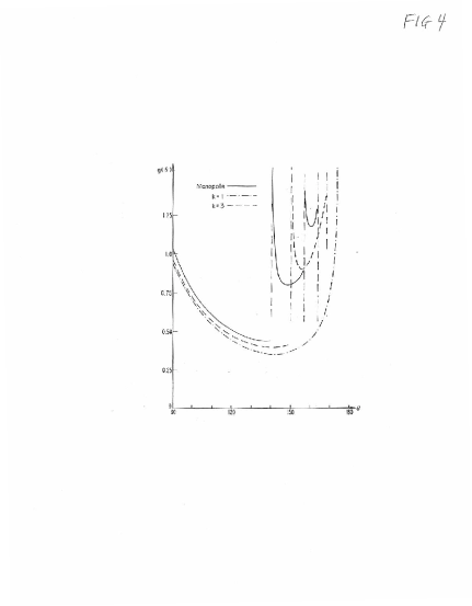
Figure 4: Classical cross section for monopole-electron and dyon-dyon scattering. Again, $k\pi=|\kappa|v_{0}/q$, while $g(\theta)=(\mu v_{0}/\kappa)^{2}(\rmd\sigma/\rmd\Omega)$.

The cross section becomes infinite in two circumstances; first, when

$$\sin\theta=0\quad(\sin\chi\neq 0),\qquad\theta=\pi,$$ (2.2dik)

we have what is called a glory. For monopole-electron scattering this occurs for

$${\chi_{g}\over 2}=1.047,\,1.318,\,1.403,\,\dots.$$ (2.2dil)

The other case in which the cross section diverges is when

$${\rmd\theta\over\rmd\chi}=0.$$ (2.2dim)

This is called a rainbow. For monopole-electron scattering this occurs at

$$\theta_{r}=140.1^{\circ},\,156.7^{\circ},\,163.5^{\circ},\,\dots.$$ (2.2din)

For small scattering angles we have the generalization of the Rutherford formula

$$\frac{\rmd\sigma}{\rmd\Omega}=\frac{1}{(2\mu v_{0})^{2}}\left\{\left(\frac{e_{1}g_{2}-e_{2}g_{1}}{c}\right)^{2}+\left(\frac{e_{1}e_{2}+g_{1}g_{2}}{v_{0}}\right)^{2}\right\}\frac{1}{(\theta/2)^{4}},\qquad\theta\ll 1.$$ (2.2dio)

Note that for electron-monopole scattering, $e_{1}=e$, $e_{2}=0$, $g_{1}=0$, $g_{2}=g$, this cross section differs from the Rutherford one for electron-electron scattering by the replacement

$$\frac{e_{2}}{v}\to\frac{g}{c}.$$ (2.2dip)

This is a universal feature which we (and others) used in our experimental analyses.

3 Quantum theory

Dirac showed in 1931 [9] that quantum mechanics was consistent with the existence of magnetic monopoles provided the quantization condition holds,

$$eg=m^{\prime}\hbar c,$$ (2.2dia)

where $m^{\prime}$ is an integer or an integer plus 1/2, which explains the quantization of electric charge. This was generalized by Schwinger to dyons:

$$e_{1}g_{2}-e_{2}g_{1}=-m^{\prime}\hbar c.$$ (2.2dib)

(Schwinger sometimes argued [33] that $m^{\prime}$ was an integer, or perhaps an even integer.) We will demonstrate these quantization conditions in the following. Henceforth in this section we shall set $\hbar=c=1$.

3.1 Vector potential

One can see where charge quantization comes from by considering quantum mechanical scattering. To define the Hamiltonian, one must introduce a vector potential, which must be singular because

$$\boldsymbol{\nabla}\cdot\mathbf{B}\neq 0\Rightarrow{\bf B}\neq\boldsymbol{\nabla}\times{\bf A}.$$ (2.2dic)

For example, a potential singular along the entire line $\bf\hat{n}$ is

$${\bf A(r)}=-\frac{g}{r}\frac{1}{2}\left(\frac{{\bf\hat{n}\times r}}{r-{\bf\hat{n}\cdot r}}-\frac{{\bf\hat{n}\times r}}{r+{\bf\hat{n}\cdot r}}\right)=-\frac{g}{r}\cot\theta\mbox{\boldmath{$\hat{\phi}$}}$$ (2.2did)

where the latter form applies if ${\bf\hat{n}=\hat{z}}$, which corresponds to the magnetic field produced by a magnetic monopole at the origin,

$${\bf B(r)}=g\frac{{\bf r}}{r^{3}}.$$ (2.2die)

In view of (2.2dic), we can write

$$\mathbf{B(r)}=\boldsymbol{\nabla}\times\mathbf{A(r)}+g\mathbf{f(r)},$$ (2.2difa)

where

$$\boldsymbol{\nabla}\cdot\mathbf{f(r)}=4\pi\delta(\mathbf{r}),$$ (2.2difb)

in which $\mathbf{f}$ has support only along the line $\mathbf{\hat{n}}$ passing through the origin. The line of singularities is called the string, and $\mathbf{f}$ is called the string function. Invariance of the theory (wavefunctions must be single-valued) under string rotations implies the charge quantization condition (2.2dia). This is a nonperturbative statement, which is proved in section 3.1.3.

3.1.1 Yang’s approach

Yang offered another approach, which is fundamentally equivalent [34, 35, 36, 37, 38, 39, 40, 41]. He insisted that there be no singularities, but rather different potentials in different but overlapping regions:

$$A^{a}_{\phi}={g\over r\sin\theta}(1-\cos\theta)={g\over r}\tan{\theta\over 2},\qquad\theta<\pi,$$ (2.2difga)

$$A^{b}_{\phi}=-{g\over r\sin\theta}(1+\cos\theta)=-{g\over r}\cot{\theta\over 2},\qquad\theta>0.$$ (2.2difgb)

These correspond to the same magnetic field, so must differ by a gradient:

$$A^{a}_{\mu}-A^{b}_{\mu}={2g\over r\sin\theta}\mbox{\boldmath{$\hat{\phi}$}}=\partial_{\mu}\lambda,$$ (2.2difgh)

where $\lambda=2g\phi.$ Requiring now that $\rme^{\rmi e\lambda}$ be single valued leads to the quantization condition, $eg=m^{\prime}$, $m^{\prime}$ a half integer.

3.1.2 Spin approach

There is also a intrinsic spin formulation, pioneered by Goldhaber [42, 43]. The energy (2.2dg),

$$E={1\over 2}\mu v^{2}+{q\over r},\qquad q=e_{1}e_{2}+g_{1}g_{2},$$ (2.2difgi)

differs by a gauge transformation from

$${\cal H}={1\over 2\mu}\left(p_{r}^{2}+{J^{2}-({\bf J\cdot\hat{r}})^{2}\over r^{2}}\right)+{q\over r},$$ (2.2difgj)

where

$${\bf J}={\bf r\times p+S},$$ (2.2difgka)

$$\mu{\bf v}={\bf p}+{{\bf S\times r}\over r^{2}}.$$ (2.2difgkb)

The quantization condition appears as

$${\bf S\cdot\hat{r}}=m^{\prime}.$$ (2.2difgkl)

The elaboration of this [44] is given in section 3.1.5.

3.1.3 Strings

Let us now discuss in detail the nonrelativistic, quantum scattering of two dyons, with electric and magnetic charges $e_{1},g_{1}$ and $e_{2},g_{2}$, respectively. The Hamiltonian for the system is

$$\mathcal{H}=\frac{1}{2}m_{1}v_{1}^{2}+\frac{1}{2}m_{2}v_{2}^{2}+\frac{q}{|\mathbf{r}_{1}-\mathbf{r}_{2}|},$$ (2.2difgkm)

where, in terms of the canonical momenta, the velocities are given by

$$m_{1}\mathbf{v}_{1}=\mathbf{p}_{1}-e_{1}\mathbf{A}_{e2}(\mathbf{r}_{1},t)-g_{1}\mathbf{A}_{m2}(\mathbf{r}_{1},t),$$ (2.2difgkna)

$$m_{2}\mathbf{v}_{2}=\mathbf{p}_{2}-e_{2}\mathbf{A}_{e1}(\mathbf{r}_{2},t)-g_{2}\mathbf{A}_{m1}(\mathbf{r}_{2},t).$$ (2.2difgknb)

The electric ($e$) and magnetic ($m$) vector potentials are

$$4\pi\mathbf{A}_{e}(\mathbf{r},t)=4\pi\boldsymbol{\nabla}\lambda_{e}(\mathbf{r},t)-\int(\rmd\mathbf{r}^{\prime})\mathbf{f(r-r^{\prime})}\times\mathbf{B}(\mathbf{r}^{\prime},t),$$ (2.2difgknoa)

$$4\pi\mathbf{A}_{m}(\mathbf{r},t)=4\pi\boldsymbol{\nabla}\lambda_{m}(\mathbf{r},t)+\int(\rmd\mathbf{r}^{\prime}){}^{*}\mathbf{f(r-r^{\prime})}\times\mathbf{E}(\mathbf{r}^{\prime},t),$$ (2.2difgknob)

with

$$\lambda_{e}(\mathbf{r},t)=\int(\rmd\mathbf{r}^{\prime})\mathbf{f(r-r^{\prime})}\cdot\mathbf{A}_{e}(\mathbf{r}^{\prime},t),$$ (2.2difgknopa)

$$\lambda_{m}(\mathbf{r},t)=\int(\rmd\mathbf{r}^{\prime}){}^{*}\mathbf{f(r-r^{\prime})}\cdot\mathbf{A}_{m}(\mathbf{r}^{\prime},t).$$ (2.2difgknopb)

Here, the functions $\mathbf{f}$ and ${}^{*}\mathbf{f}$ represent the strings and must satisfy

$$\boldsymbol{\nabla}\cdot{}^{(*)}\mathbf{f(r-r^{\prime})}=4\pi\delta(\mathbf{r-r^{\prime}}).$$ (2.2difgknopq)

A priori, $\mathbf{f}$ and ${}^{*}\mathbf{f}$ need not be related, and could be different for each source. So, for the case of dyon-dyon scattering, it would seem that four independent strings are possible.

The first condition we impose on the Schrödinger equation,

$$\mathcal{H}\Psi=E\Psi,$$ (2.2difgknopr)

is that it separates when center-of-mass and relative coordinates are employed, which implies

$$e_{1}\mathbf{A}_{e2}(\mathbf{r}_{1},t)=-g_{2}\mathbf{A}_{m1}(\mathbf{r}_{2},t)\equiv e_{1}g_{2}\boldsymbol{\mathcal{A}}(\mathbf{r}),$$ (2.2difgknopsa)

$$e_{2}\mathbf{A}_{e1}(\mathbf{r}_{2},t)=-g_{1}\mathbf{A}_{m2}(\mathbf{r}_{1},t)\equiv e_{2}g_{1}\boldsymbol{\mathcal{A}}^{\prime}(\mathbf{r}),$$ (2.2difgknopsb)

where $\mathbf{r}=\mathbf{r}_{1}-\mathbf{r}_{2}$. Correspondingly, there are relations between the various string functions,

$${}^{*}\mathbf{f}_{1}(\mathbf{x})=-\mathbf{f}_{2}(-\mathbf{x}),\qquad{}^{*}\mathbf{f}_{2}(\mathbf{x})=-\mathbf{f}_{1}(-\mathbf{x}),$$ (2.2difgknopst)

leaving only two independent ones. The Hamiltonian for the relative coordinates now reads

$$\mathcal{H}=\frac{1}{2\mu}[\mathbf{p}-e_{1}g_{2}\boldsymbol{\mathcal{A}}(\mathbf{r})+e_{2}g_{1}\boldsymbol{\mathcal{A}}^{\prime}(\mathbf{r})]^{2}+\frac{q}{r},$$ (2.2difgknopsu)

where $\mu$ is the reduced mass.

If we further require that only one vector potential be present, $\boldsymbol{\mathcal{A}}=\boldsymbol{\mathcal{A}}^{\prime}$, so that only the antisymmetric combination of electric and magnetic charges occurring in (2.2dib) appears, one more relation is obtained between the two $\mathbf{f}$ functions,

$$\mathbf{f}_{2}(\mathbf{x})=-\mathbf{f}_{1}(-\mathbf{x}).$$ (2.2difgknopsv)

Notice that (2.2difgknopsv) possesses two types of solutions.

• There is a single string, necessarily infinite, satisfying

  $$\mathbf{f}(\mathbf{x})=-\mathbf{f}(-\mathbf{x}).$$ (2.2difgknopsw)

  Then it is easily seen that the vector potential transforms the same way as charges and currents do under duality transformations (2.2b). This is the so-called symmetric case.

• There are two strings, necessarily semi-infinite, which are negative reflections of each other.

If identical semi-infinite strings are employed, so that $\boldsymbol{\mathcal{A}}\neq\boldsymbol{\mathcal{A}}^{\prime}$, the individual charge products $e_{1}g_{2}$ and $e_{2}g_{1}$ occur in the dynamics. The singularities of $\boldsymbol{\mathcal{A}}$ and $\boldsymbol{\mathcal{A}}^{\prime}$ lie on lines parallel and antiparallel to the strings, respectively. We will see the consequences for the charge quantization condition of these different choices in the following.

For now, we return to the general situation embodied in (2.2difgknopsu). For simplicity, we choose the string associated with $\boldsymbol{\mathcal{A}}$ to be a straight line lying along the direction $\bf\hat{n}$,

$$\boldsymbol{\mathcal{A}}=\cases{-\frac{1}{r}\frac{\mathbf{\hat{n}\times r}}{r-(\mathbf{\hat{n}\cdot r})},&\mbox{semi-infinite}\\ -\frac{1}{r}\frac{1}{2}\left(\frac{\mathbf{\hat{n}\times r}}{r-(\mathbf{\hat{n}\cdot r})}-\frac{\mathbf{\hat{n}\times r}}{r+(\mathbf{\hat{n}\cdot r})}\right),&\mbox{infinite}}.$$ (2.2difgknopsx)

This result is valid in the gauge in which $\lambda_{e(m)}$ [(2.2difgknopa), (2.2difgknopb)] is equal to zero. Without loss of generality, we will take $\boldsymbol{\mathcal{A}}^{\prime}$ to be given by (2.2difgknopsx) with $\mathbf{\hat{n}\to\hat{z}}$, which corresponds to taking the string associated with $\boldsymbol{\mathcal{A}}^{\prime}$ to point along the $-z$ axis, $\mathbf{f}_{1}\propto-\mathbf{\hat{z}}$.

We now wish to convert the resulting Hamiltonian, $\mathcal{H}$, into a form $\mathcal{H}^{\prime}$ in which all the singularities lie along the $z$ axis. It was in that case that the Schrödinger equation was solved in [19], as described in section 3.2, yielding the quantization condition (2.2dib). This conversion is effected by a unitary transformation [45] (essentially a gauge transformation),

$$\mathcal{H}^{\prime}=\rme^{\rmi\Lambda}\mathcal{H}\rme^{-\rmi\Lambda}.$$ (2.2difgknopsy)

The differential equation determining $\Lambda$ is

$$\boldsymbol{\nabla}\Lambda=e_{1}g_{2}[\boldsymbol{\mathcal{A}}^{\prime}(\mathbf{r})-\boldsymbol{\mathcal{A}}(\mathbf{r})].$$ (2.2difgknopsz)

We take $\mathbf{\hat{n}}$ to be given by

$$\mathbf{\hat{n}}=\sin\chi\cos\psi\mathbf{\hat{x}}+\sin\chi\sin\psi\mathbf{\hat{y}}+\cos\chi\mathbf{\hat{z}},$$ (2.2difgknopsaa)

and use spherical coordinates [$\mathbf{r}=(r,\theta,\phi)$], to find

$$\Lambda=-e_{1}g_{2}\beta(\mathbf{\hat{n},r}),$$ (2.2difgknopsab)

where, for the semi-infinite string (Dirac)

$$\beta_{D}=\phi-\psi+(\cos\theta-\cos\chi)F_{-}(\theta,\phi-\psi,\chi)-2\pi\eta(\chi-\eta),$$ (2.2difgknopsaca)

and for the infinite string (Schwinger)

$$\beta_{S}=\frac{1}{2}\left[(\cos\theta-\cos\chi)F_{-}(\theta,\phi-\psi,\chi)+(\cos\theta+\cos\chi)F_{+}(\theta,\phi-\psi,\chi)-2\pi\eta(\chi-\theta)\right].$$

(2.2difgknopsacb)

The functions occurring here are

$$F_{\pm}(\theta,\alpha,\chi)=\int_{0}^{\alpha}\frac{\rmd\phi^{\prime}}{1\pm\cos\chi\cos\theta\pm\sin\chi\sin\theta\cos\phi^{\prime}}$$

$$=\frac{2\epsilon(\alpha)}{|\cos\theta\pm\cos\chi|}\arctan\left[\left(\frac{1\pm\cos(\chi+\theta)}{1\pm\cos(\chi-\theta)}\right)^{1/2}\tan\frac{|\alpha|}{2}\right],$$ (2.2difgknopsacad)

where the arctangent is not defined on the principal branch, but is chosen such that $F_{\pm}(\theta,\alpha,\chi)$ is a monotone increasing function of $\alpha$. The step functions occurring here are defined by

$$\eta(\xi)=\cases{1,&$\xi>0$,\\ 0,&$\xi<0$,}$$ (2.2difgknopsacaea)

$$\epsilon(\xi)=\cases{1,&$\xi>0$,\\ -1,&$\xi<0$.}$$ (2.2difgknopsacaeb)

The phases, $\beta_{D}$ and $\beta_{S}$, satisfy the appropriate differential equation (2.2difgknopsz), for $\theta\neq\chi$ (as well as $\theta\neq\pi-\chi$ for $\beta_{S}$) and are determined up to constants. The step functions $\eta$ are introduced here in order to make $\rme^{\rmi\Lambda}$ continuous at $\theta=\chi$ and $\pi-\chi$, as will be explained below. We now observe that

$$F_{\pm}(\theta,2\pi+\alpha,\chi)-F_{\pm}(\theta,\alpha,\chi)=\frac{2\pi}{|\cos\theta\pm\cos\chi|},$$ (2.2difgknopsacaeaf)

so that the wavefunction

$$\Psi=\rme^{-\rmi\Lambda}\Psi^{\prime},$$ (2.2difgknopsacaeag)

where $\Psi^{\prime}$ is the solution to the Schrödinger equation with the singularity on the $z$ axis, is single-valued under the substitution $\phi\to\phi+2\pi$ when the quantization condition (2.2dia) is satisfied.

Notice that integer quantization follows when an infinite string is used while a semi-infinite string leads to half-integer quantization, since $\beta_{S}$ changes by a multiple of $2\pi$ when $\phi\to\phi+2\pi$, while $\beta_{D}$ changes by an integer multiple of $4\pi$. Notice that $\beta_{D}$ possesses a discontinuity, which is a multiple of $4\pi$, at $\theta=\chi$, while $\beta_{S}$ possesses discontinuities, which are multiples of $2\pi$, at $\theta=\chi$, $\pi-\chi$. In virtue of the above-derived quantization conditions, $\rme^{\rmi\Lambda}$ is continuous everywhere. Correspondingly, the unitary operator $\rme^{\rmi\Lambda}$, which relates solutions of Schrödinger equations with different vector potentials, is alternatively viewed as a gauge transformation relating physically equivalent descriptions of the same system, since it converts one string into another. [Identical arguments applied to the case when only one vector potential is present leads to the condition (2.2dib), where $m^{\prime}$ is an integer, or an integer plus one-half, for infinite and semi-infinite strings, respectively.]

It is now a simple application of the above results to transform a system characterized by a single vector potential with an infinite string along the direction $\bf\hat{n}$ into one in which the singularity line is semi-infinite and lies along the $+z$ axis. This can be done in a variety of ways; particularly easy is to break the string at the origin and transform the singularities to the $z$ axis. Making use of (2.2difgknopsab) with $e_{1}g_{2}\to-m^{\prime}/2$ and (2.2difgknopsaca) for $\bf\hat{n}$ and $-\mathbf{\hat{n}}$, we find

$$\Lambda=m^{\prime}\beta^{\prime}_{S}(\mathbf{\hat{n},r})\qquad\mbox{with}\qquad\beta_{S}^{\prime}=\phi-\psi+\beta_{S}.$$ (2.2difgknopsacaeah)

In particular, we can relate the wavefunctions for infinite and semi-infinite singularity lines on the $z$ axis by setting $\chi=0$ in (2.2difgknopsacaeah),

$$\beta^{\prime}_{S}=\phi-\psi,$$ (2.2difgknopsacaeai)

so

$$\Psi(\mbox{infinite})=\rme^{-\rmi m^{\prime}(\phi-\psi)}\Psi(\mbox{semi-infinite}).$$ (2.2difgknopsacaeaj)

Note that (2.2difgknopsacaeaj) or (2.2difgknopsacaeah) reiterates that an infinite string requires integer quantization.

3.1.4 Scattering

In the above subsection, we related the wavefunction when the string lies along the direction $\mathbf{\hat{n}}$ with that when the string lies along the $z$ axis. When there is only a single vector potential (which, for simplicity, we will assume throughout the following), this relation is

$$\Psi_{\bf\hat{n}}=\rme^{-\rmi m^{\prime}\beta(\mathbf{\hat{n},r})}\Psi^{\prime},$$ (2.2difgknopsacaeak)

where $\beta$ is given by (2.2difgknopsaca), (2.2difgknopsacb), or (2.2difgknopsacaeah) for the various cases. For concreteness, if we take $\Psi^{\prime}$ to be a state corresponding to a semi-infinite singularity line along the $+z$ axis, then $\beta$ is either $\beta_{D}$ (2.2difgknopsaca) or $\beta_{S}^{\prime}$ (2.2difgknopsacaeah) depending on whether the singularity characterized by $\bf\hat{n}$ is semi-infinite or infinite. By means of (2.2difgknopsacaeak), we can easily build up the relation between solutions corresponding to two arbitrarily oriented strings, with $\bf\hat{n}$ and $\bf\hat{n}^{\prime}$ say,

$$\Psi_{\bf\hat{n}^{\prime}}=\rme^{-\rmi m^{\prime}(\beta(\mathbf{\hat{n}^{\prime},r})-\beta(\mathbf{\hat{n},r}))}\Psi_{\bf\hat{n}},$$ (2.2difgknopsacaeal)

which expresses the gauge covariance properties of the wavefunctions.

For scattering, we require a solution that consists of an incoming plane wave and an outgoing spherical wave. We will consider an eigenstate of $\mathbf{J\cdot\hat{k}}$ where $\mathbf{J}$ is the total angular momentum

$$\mathbf{J}=\mathbf{r}\times(\mathbf{p}+m^{\prime}\boldsymbol{\mathcal{A}}_{\bf\hat{n}})+m^{\prime}\mathbf{\hat{r}},$$ (2.2difgknopsacaeam)

and $\mathbf{\hat{k}}$ is the unit vector in the direction of propagation of the incoming wave (not necessarily the $z$ axis). This state cannot be an eigenstate of $\mathbf{\hat{k}\cdot(r\times p)}$, since this operator does not commute with the Hamiltonian. However, since

$$\rme^{\rmi\Lambda}\mathbf{\hat{k}\cdot J}\rme^{-\rmi\Lambda}=\mathbf{\hat{k}\cdot(r\times p)}-m^{\prime},$$ (2.2difgknopsacaeana)

for a reorientation of the string from $$\bf\hat{n} \bf\hat{k}$$ to ,

$$\Lambda=m^{\prime}[\beta(\mathbf{\hat{n},r})-\beta_{D}(\mathbf{\hat{k},r})],$$ (2.2difgknopsacaeanb)

because

$$\frac{\mathbf{\hat{k}\cdot(\hat{r}\times(\hat{k}\times\hat{r}))}}{1-\mathbf{\hat{k}\cdot\hat{r}}}=1+\mathbf{\hat{k}\cdot\hat{r}},$$ (2.2difgknopsacaeanao)

the incoming state with eigenvalue [46]

$$(\mathbf{\hat{k}\cdot J})^{\prime}=-m^{\prime}$$ (2.2difgknopsacaeanap)

is simply related to an ordinary modified plane wave [$\eta$ is defined below in (2.2difgknopsacaeanau)]

$$\Psi_{\rm in}=\rme^{-\rmi\Lambda}\exp\left\{\rmi\left[\mathbf{k\cdot r}+\eta\ln(kr-\mathbf{k\cdot r})\right]\right\}.$$ (2.2difgknopsacaeanaq)

This state exhibits the proper gauge covariance under reorientation of the string.

The asymptotic form of the wavefunction is

$$\Psi\sim\rme^{-\rmi m^{\prime}\beta(\mathbf{\hat{n},r})}\sum_{j\bar{m}}A_{kj\bar{m}}\mathcal{Y}^{m^{\prime}}_{j\bar{m}}(\mathbf{\hat{r}})\rme^{\rmi m^{\prime}\phi}\frac{1}{kr}\sin\left(kr-\eta\ln 2kr-\frac{\pi}{2}L+\delta_{L}\right),\qquad r\to\infty.$$ (2.2difgknopsacaeanar)

The summation in (2.2difgknopsacaeanar) is the general from of the solution when the singularity line is semi-infinite, extending along the $+z$ axis. In particular, $\mathcal{Y}^{m^{\prime}}_{j\bar{m}}$ is a generalized spherical harmonic, which is another name for the rotation matrices in quantum mechanics [$\mathbf{\hat{r}}=(\theta,\phi)$],

$$\langle jm^{\prime}|\rme^{\rmi\psi J_{3}}\rme^{\rmi\theta J_{2}}\rme^{\rmi\phi J_{3}}|jm\rangle=\rme^{\rmi m^{\prime}\psi}\frac{1}{\sqrt{2j+1}}\mathcal{Y}^{m^{\prime}}_{jm}(\mathbf{\hat{r}})=\rme^{\rmi m^{\prime}\psi}U_{m^{\prime}m}^{(j)}(\theta)\rme^{\rmi m\phi},$$ (2.2difgknopsacaeanas)

$\delta_{L}$ is the Coulomb phase shift for noninteger $L$,

$$\delta_{L}=\mbox{arg}\,\Gamma(L+1+\rmi\eta),$$ (2.2difgknopsacaeanat)

and

$$L+\frac{1}{2}=\sqrt{\left(j+\frac{1}{2}\right)^{2}-m^{\prime 2}},\qquad\eta=\frac{\mu q}{k},\qquad q=e_{1}e_{2}+g_{1}g_{2}.$$ (2.2difgknopsacaeanau)

Upon defining the outgoing wave by

$$\Psi\sim\rme^{-\rmi\Lambda}\left(\rme^{\rmi[\mathbf{k\cdot r}+\eta\ln(kr-\mathbf{k\cdot r})]}+\Psi_{\rm out}\right),$$ (2.2difgknopsacaeanav)

where $\Lambda$ is given by (2.2difgknopsacaeanb), we find that

$$\Psi_{\rm out}=\frac{1}{r}\rme^{\rmi(kr-\eta\ln kr)}\rme^{\rmi m^{\prime}\gamma}f(\bar{\theta}).$$ (2.2difgknopsacaeanaw)

In terms of the scattering angle, $\bar{\theta}$, which is the angle between $\mathbf{k}$ and $\mathbf{r}$, the scattering amplitude is

$$2\rmi kf(\bar{\theta})=\sum_{j=|m^{\prime}|}^{\infty}\sqrt{2j+1}\mathcal{Y}^{m^{\prime}}_{jm^{\prime}}(\pi-\bar{\theta},0)\rme^{-\rmi(\pi L-2\delta_{L})}.$$ (2.2difgknopsacaeanax)

The extra phase in (2.2difgknopsacaeanaw) is given by (where $\mathbf{\hat{k}}$ characterized by $\theta^{\prime}$, $\phi^{\prime}$ and $-\mathbf{\hat{k}}$ by $\pi-\theta^{\prime}$, $\phi^{\prime}\pm\pi$)

$$\gamma=\beta_{D}(\mathbf{\hat{k},-\hat{k}})+\phi-\phi^{\prime}\mp\pi-\beta_{D}(\mathbf{\hat{k},r})+\bar{\phi},$$ (2.2difgknopsacaeanay)

where

$$\arctan\frac{1}{2}\bar{\phi}=\frac{\cos\left(\frac{\theta+\pi-\theta^{\prime}}{2}\right)\sin\left(\frac{\phi-\phi^{\prime}\mp\pi}{2}\right)}{\cos\left(\frac{\theta-\pi+\theta^{\prime}}{2}\right)\cos\left(\frac{\phi-\phi^{\prime}\mp\pi}{2}\right)}.$$ (2.2difgknopsacaeanaz)

Straightforward evaluation shows that

$$\frac{\gamma}{2}=0\,\,(\mbox{mod}\,2\pi),$$ (2.2difgknopsacaeanba)

so that there is no additional phase factor in the outgoing wave.

3.1.5 Spin

Classically, the electromagnetic field due to two dyons at rest carries angular momentum, as in section 2.2,

$$\mathbf{S}_{\rm classical}=m^{\prime}\mathbf{\hat{r}}.$$ (2.2difgknopsacaeanbb)

A quantum-mechanical transcription of this fact allows us to replace the nonrelativistic description explored above, in which the interaction is through the vector potentials (apart from the Coulomb term), by one in which the particles interact with an intrinsic spin. The derivation of the magnetic charge problem from this point of view seems first to have carried out by Goldhaber [42] in a simplified context, and was revived in the context of ’t Hooft-Polyakov monopoles [13, 14, 47, 48, 15, 46], where the spin is called “isospin.”

Before introducing the notion of spin, we first consider the angular momentum of the actual dyon problem. For simplicity we will describe the interaction between two dyons in terms of a single vector potential $\boldsymbol{\mathcal{A}}$, and an infinite string satisfying (2.2difgknopsw). (The other cases are simple variations on what we do here, and the consequences for charge quantization are the same as found in section 3.1.3.) Then the relative momentum of the system is

$$\mathbf{p}=\mu\mathbf{v}-m^{\prime}\boldsymbol{\mathcal{A}}.$$ (2.2difgknopsacaeanbc)

Since from (2.2difgknoa), (2.2difgknob), we have the result in (2.2difa), or

$$\boldsymbol{\nabla}\times\boldsymbol{\mathcal{A}}=\frac{\mathbf{r}}{r^{3}}-\mathbf{f(r)},$$ (2.2difgknopsacaeanbd)

we have the following commutation property valid everywhere,

$$\mu\mathbf{v}\times\mu\mathbf{v}=-\rmi m^{\prime}\left[\frac{\mathbf{r}}{r^{3}}-\mathbf{f(r)}\right].$$ (2.2difgknopsacaeanbe)

Motivated by the classical situation, we assert that the total angular momentum operator is (2.2difgknopsacaeam), or

$$\mathbf{J}=\mathbf{r}\times\mu\mathbf{v}+m^{\prime}\mathbf{\hat{r}}.$$ (2.2difgknopsacaeanbf)

This is confirmed [11] by noting that, almost everywhere, $\mathbf{J}$ is the generator of rotations:

$$\frac{1}{\rmi}[\mathbf{r,J}\cdot\delta\boldsymbol{\omega}]=\delta\boldsymbol{\omega}\times\mathbf{r},$$ (2.2difgknopsacaeanbga)

$$\frac{1}{\rmi}[\mu\mathbf{v},\mathbf{J}\cdot\delta\boldsymbol{\omega}]=\delta\boldsymbol{\omega}\times\mu\mathbf{v}-m^{\prime}\mathbf{f(r)}\times(\delta\boldsymbol{\omega}\times\mathbf{r}),$$ (2.2difgknopsacaeanbgb)

where $\delta\boldsymbol{\omega}$ stands for an infinitesimal rotation. The presence of the extra term in (2.2difgknopsacaeanbgb) is consistent only because of the quantization condition [33]. For example, consider the effect of a rotation on the time evolution operator,

$$\rme^{-\rmi\mathbf{J}\cdot\delta\boldsymbol{\omega}}\exp\left[-\rmi\int\rmd t\,\mathcal{H}\right]\rme^{\rmi\mathbf{J}\cdot\delta\boldsymbol{\omega}}=\exp\left[-\rmi\int\rmd t\left(\mathcal{H}+\delta\mathcal{H}\right)\right],$$ (2.2difgknopsacaeanbgbh)

where

$$\delta\mathcal{H}=\rmi[\mathcal{H},\mathbf{J}\cdot\delta\boldsymbol{\omega}]=m^{\prime}\mathbf{v}\cdot[\mathbf{f(r)\times\delta r}],\qquad\delta\mathbf{r}=\delta\boldsymbol{\omega}\times\mathbf{r}.$$ (2.2difgknopsacaeanbgbi)

Using the representation for the string function,

$$\mathbf{f(r)}=4\pi\int_{C}\rmd\mathbf{x}\frac{1}{2}\left[\delta(\mathbf{r-x})-\delta(\mathbf{r+x})\right],$$ (2.2difgknopsacaeanbgbj)

where $C$ is any contour starting at the origin and extending to infinity, and the notation $\rmd t\mathbf{v}=\rmd\mathbf{r}$, we have

$$-\rmi\int\rmd t\,\delta\mathcal{H}=-\rmi m^{\prime}4\pi\int\rmd\mathbf{r}\cdot(\rmd\mathbf{x}\times\delta\mathbf{r})\frac{1}{2}\left[\delta(\mathbf{r-x})-\delta(\mathbf{r+x})\right].$$ (2.2difgknopsacaeanbgbk)

Since the possible values of the integral are 0, $\pm\frac{1}{2}$, $\pm 1$, the unitary time development operator is unaltered by a rotation only if $m^{\prime}$ is an integer. (Evidently, half-integer quantization results from the use of a semi-infinite string.)

Effectively, then, $\mathbf{J}$ satisfies the canonical angular momentum commutation relations (see also section 3.1.6)

$$\frac{1}{\rmi}\mathbf{J\times J=J},$$ (2.2difgknopsacaeanbgbl)

and is a constant of the motion,

$$\frac{\rmd}{\rmd t}\mathbf{J}=\frac{1}{\rmi}[\mathcal{H},\mathbf{J}]=0.$$ (2.2difgknopsacaeanbgbm)

And, corresponding to the classical field angular momentum (2.2difgknopsacaeanbb), the component of $\mathbf{J}$ along the line connecting the two dyons, $m^{\prime}$, should be an integer.

The identification of $m^{\prime}$ as an angular momentum component invites us to introduce an independent spin operator $\mathbf{S}$. We do this by first writing [11], as anticipated in (2.2difgkl), (2.2difgkb),

$$m^{\prime}=\mathbf{S\cdot\hat{r}},$$ (2.2difgknopsacaeanbgbna)

and

$$\mu\mathbf{v}=\mathbf{p}+\frac{\mathbf{S\times r}}{r^{2}},$$ (2.2difgknopsacaeanbgbnb)

which, when substituted into (2.2difgknopsacaeanbf) yields (2.2difgka),

$$\mathbf{J=r\times p+S}.$$ (2.2difgknopsacaeanbgbnbo)

We now ascribe independent canonical commutation relations to $\mathbf{S}$, and regard (2.2difgknopsacaeanbgbna) as an eigenvalue statement. The consistency of this assignment is verified by noting that the commutation property

$$\mu\mathbf{v}\times\mu\mathbf{v}=-\rmi m^{\prime}\frac{\mathbf{r}}{r^{3}}$$ (2.2difgknopsacaeanbgbnbp)

holds true, and that $\mathbf{S\cdot\hat{r}}$ is a constant of the motion,

$$[\mathbf{S\cdot\hat{r}},\mu\mathbf{v}]=0.$$ (2.2difgknopsacaeanbgbnbq)

In this angular momentum description, the Hamiltonian, (2.2difgknopsu), can be written in the form

$$\mathcal{H}=\frac{1}{2\mu}\left[p^{2}+\frac{2\mathbf{S\cdot L}}{r^{2}}+\frac{\mathbf{S}^{2}-(\mathbf{S\cdot\hat{r}})^{2}}{r^{2}}\right]+\frac{q}{r},$$ (2.2difgknopsacaeanbgbnbr)

in terms of the orbital angular momentum,

$$\mathbf{L=r\times p}.$$ (2.2difgknopsacaeanbgbnbs)

The total angular momentum $\mathbf{J}$ appears when the operator

$$p_{r}^{2}=\frac{1}{r^{2}}\left[(\mathbf{r\cdot p})^{2}+\frac{1}{\rmi}\mathbf{r\cdot p}\right],$$ (2.2difgknopsacaeanbgbnbt)

is introduced into the Hamiltonian

$$\mathcal{H}=\frac{1}{2\mu}\left[p_{r}^{2}+\frac{\mathbf{J}^{2}-(\mathbf{J\cdot\hat{r}})^{2}}{r^{2}}\right]+\frac{q}{r}.$$ (2.2difgknopsacaeanbgbnbu)

In an eigenstate of $\mathbf{J}^{2}$ and $\mathbf{J\cdot\hat{r}}$.

$$(\mathbf{J}^{2})^{\prime}=j(j+1),\qquad(\mathbf{J\cdot\hat{r}})^{\prime}=m^{\prime},$$ (2.2difgknopsacaeanbgbnbv)

(2.2difgknopsacaeanbgbnbu) yields the radial Schrödinger equation (2.2difgknopsacaeanbgbncdcecodgdxa) solved in section 3.2. This modified formulation, only formally equivalent to our starting point, makes no reference to a vector potential or string.

We now proceed to diagonalize the $\mathbf{S}$ dependence of the Hamiltonian, (2.2difgknopsacaeanbgbnbr) or (2.2difgknopsacaeanbgbnbu), subject to the eigenvalue constraint

$$(\mathbf{S\cdot\hat{r}})^{\prime}=m^{\prime}.$$ (2.2difgknopsacaeanbgbnbw)

This is most easily done by diagonalizing [46] the angular momentum operator (2.2difgknopsacaeanbgbnbo). In order to operate in a framework sufficiently general to include our original symmetrical starting point, we first write $\mathbf{S}$ as the sum of two independent spins

$$\mathbf{S}=\mathbf{S}_{a}+\mathbf{S}_{b}.$$ (2.2difgknopsacaeanbgbnbx)

We then subject $\mathbf{J}$ to a suitable unitary transformation [42]

$$\mathbf{J}^{\prime}=U\mathbf{J}U^{-1},$$ (2.2difgknopsacaeanbgbnby)

where

$$U=\exp[\rmi(\mathbf{S}_{a}\cdot\hat{\boldsymbol{\phi}})\theta]\exp[\rmi(\mathbf{S}_{b}\cdot\hat{\boldsymbol{\phi}})(\theta-\pi)],$$ (2.2difgknopsacaeanbgbnbz)

which rotates $\mathbf{S}_{a,b}\cdot\mathbf{\hat{r}}$ into $\pm(\mathbf{S}_{a,b})_{3}$. This transformation is easily carried out by making use of the representation in terms of Euler angles,

$$\exp(\rmi\mathbf{S}\cdot\boldsymbol{\phi}\,\theta)=\exp(-\rmi\phi S_{3})\exp(\rmi\theta S_{2})\exp(\rmi\phi S_{3}).$$ (2.2difgknopsacaeanbgbnca)

The general form of the transformed angular momentum,

$$\mathbf{J}^{\prime}=\mathbf{r}\times\left[\mathbf{p}+\frac{\hat{\boldsymbol{\phi}}}{r}\sin\theta\left(\frac{S_{a3}}{1+\cos\theta}+\frac{S_{b3}}{1-\cos\theta}\right)\right]+\mathbf{\hat{r}}(\mathbf{S}_{a}-\mathbf{S}_{b})^{\prime}_{3},$$ (2.2difgknopsacaeanbgbncb)

is subject, a priori, only to the constraint (2.2difgknopsacaeanbgbnbw), or

$$(\mathbf{S}_{a}-\mathbf{S}_{b})^{\prime}_{3}=m^{\prime}.$$ (2.2difgknopsacaeanbgbncc)

We recover the unsymmetrical and symmetrical formulations by imposing the following supplementary eigenvalue conditions:

$$(1):\qquad S_{a3}^{\prime}=0,$$ (2.2difgknopsacaeanbgbncda)

$$(2):\qquad(\mathbf{S}_{a}+\mathbf{S}_{b})^{\prime}_{3}=0.$$ (2.2difgknopsacaeanbgbncdb)

These yield the angular momentum in the form (2.2difgknopsacaeanbf) or (2.2difgknopsacaeam), the vector potential appearing there being, respectively,

$$(1):\qquad\boldsymbol{\mathcal{A}}=-\frac{\hat{\boldsymbol{\phi}}}{r}\cot\frac{\theta}{2},$$ (2.2difgknopsacaeanbgbncdcea)

$$(2):\qquad\boldsymbol{\mathcal{A}}=-\frac{\hat{\boldsymbol{\phi}}}{r}\cot\theta,$$ (2.2difgknopsacaeanbgbncdceb)

which are (2.2difgknopsx) with $\mathbf{\hat{n}=\hat{z}}$. [See also (2.2difgb), (2.2did).]

The effect of this transformation on the Hamiltonian is most easily seen from the form (2.2difgknopsacaeanbgbnbu),

$$U\left[p_{r}^{2}+\frac{J^{2}-(\mathbf{J\cdot{\hat{r}}})^{2}}{r^{2}}\right]U^{-1}=p_{r}^{2}+\frac{1}{r^{2}}(\mathbf{r\times\mu v})^{2}=(\mu\mathbf{v})^{2},$$ (2.2difgknopsacaeanbgbncdcecf)

making use of (2.2difgknopsacaeanbgbnbt), or

$$\mathcal{H}^{\prime}=U\mathcal{H}U^{-1}=\frac{1}{2}\mu v^{2}+\frac{q}{r}.$$ (2.2difgknopsacaeanbgbncdcecg)

So by means of the transformation given in (2.2difgknopsacaeanbgbnbz) we have derived the explicit magnetic charge problem, expressed in terms of $\mathbf{J}^{\prime}$ and $\mathcal{H}^{\prime}$, from the implicit formulation in terms of spin. These transformations are not really gauge transformations, because the physical dyon theory is defined only after the eigenvalue conditions (2.2difgknopsacaeanbgbncc) and (2.2difgknopsacaeanbgbncda)–(2.2difgknopsacaeanbgbncdb) are imposed. The unsymmetrical condition (1), (2.2difgknopsacaeanbgbncda), gives rise to the Dirac formulation of magnetic charge, with a semi-infinite singularity line, and, from (2.2difgknopsacaeanbgbncc), $m^{\prime}$ either integer or half-integer. The symmetrical condition (2), (2.2difgknopsacaeanbgbncdb) gives the Schwinger formulation: An infinite singularity line [with (2.2difgknopsw) holding], and integer quantization of $m^{\prime}$. These correlations, which follow directly from the commutation properties of angular momentum (the group structure), are precisely the conditions required for the consistency of the magnetic charge theory, as we have seen in section 3.1.3.

Even though the individual unitary operators $U$ are not gauge transformations, a sequence of them, which serves to reorient the string direction, is equivalent to such a transformation. For example, if we formally set $\mathbf{S}_{a}=0$ in (2.2difgknopsacaeanbgbnbz),

$$U_{(1)}=\exp(\rmi\mathbf{S}\cdot\hat{\boldsymbol{\phi}}(\theta-\pi)],$$ (2.2difgknopsacaeanbgbncdcech)

we have the transformation which generates a vector potential with singularity along the positive $z$ axis, (2.2difgknopsacaeanbgbncdcea), while

$$U_{(2)}=\exp[\rmi\mathbf{S\cdot\hat{u}}_{2}(\Theta-\pi)]$$ (2.2difgknopsacaeanbgbncdceci)

generates a vector potential with singularity along $\mathbf{\hat{n}}$, the first form in (2.2difgknopsx), where $\Theta$ is the angle between $\mathbf{\hat{n}}$ and $\mathbf{r}$,

$$\cos\Theta=\cos\theta\cos\chi+\sin\theta\sin\chi\cos(\phi-\psi)$$ (2.2difgknopsacaeanbgbncdcecj)

[the coordinates of $\mathbf{\hat{n}}$ are given by (2.2difgknopsaa)], and

$$\mathbf{\hat{u}}_{2}=\frac{\mathbf{\hat{n}\times r}}{|\mathbf{\hat{n}\times r}|}.$$ (2.2difgknopsacaeanbgbncdceck)

The transformation which carries (2.2difgknopsacaeanbgbncdcea) into the first form in (2.2difgknopsx) is

$$U_{(12)}=U^{\vphantom{1}}_{(2)}U^{-1}_{(1)}.$$ (2.2difgknopsacaeanbgbncdcecl)

Since $U_{(12)}$ reorients the string from the direction $\mathbf{\hat{z}}$ to the direction $\mathbf{\hat{n}}$, it must have the form

$$U_{(12)}=\exp(\rmi\mathbf{S\cdot\hat{n}}\Phi)\exp(-\rmi\mathbf{S}\cdot\hat{\boldsymbol{\psi}}\chi).$$ (2.2difgknopsacaeanbgbncdcecm)

The angle of rotation about the $\mathbf{n}$ axis, $\Phi$, is most easily determined by considering the spin-1/2 case $\mathbf{S}=\frac{1}{2}\boldsymbol{\sigma}$, and introducing a right-handed basis,

$$\mathbf{\hat{u}}_{1}=\mathbf{\hat{n}},\qquad\mathbf{\hat{u}}_{2}=\frac{\mathbf{\hat{n}\times r}}{|\mathbf{\hat{n}\times r}|},\qquad\mathbf{\hat{u}}_{3}=\mathbf{\hat{n}\times\hat{u}}_{2}.$$ (2.2difgknopsacaeanbgbncdcecn)

Then straightforward algebra yields

$$\cos\frac{1}{2}\Phi=\frac{\sin\frac{1}{2}\theta\cos\frac{1}{2}\chi-\cos\frac{1}{2}\theta\sin\frac{1}{2}\chi\cos(\phi-\psi)}{\sin\frac{1}{2}\Theta},$$ (2.2difgknopsacaeanbgbncdcecoa)

$$\sin\frac{1}{2}\Phi=\frac{-\cos\frac{1}{2}\theta\sin\frac{1}{2}\chi\sin(\phi-\psi)}{\sin\frac{1}{2}\Theta}.$$ (2.2difgknopsacaeanbgbncdcecob)

The corresponding transformation carrying the vector potential with singularities along the negative $z$ axis [(2.2difgknopsacaeanbgbncdcea) with $\theta\to\theta-\pi$], into the vector potential with singularities along the direction of $-\mathbf{\hat{n}}$ [the first form in (2.2difgknopsx) with $\mathbf{\hat{n}\to-\hat{n}}$], are obtained from (2.2difgknopsacaeanbgbncdcecm) and (2.2difgknopsacaeanbgbncdcecoa)–(2.2difgknopsacaeanbgbncdcecob) [see also (2.2difgknopsacaeanbgbncdcech) and (2.2difgknopsacaeanbgbncdceci)] by the substitutions

$$\theta\to\theta+\pi,\qquad\Theta\to\Theta+\pi.$$ (2.2difgknopsacaeanbgbncdcecocp)

The combination of these two cases gives the transformation of the infinite string, of which (2.2difgknopsacaeanbgbnbz) is the prototype.

Since the effect of $\exp(-\rmi\mathbf{S}\cdot\hat{\boldsymbol{\psi}}\chi)$ is completely given by

$$\exp(-\rmi\mathbf{S}\cdot\hat{\boldsymbol{\psi}}\chi)S_{3}\exp(\rmi\mathbf{S}\cdot\hat{\boldsymbol{\psi}}\chi)=\mathbf{S\cdot\hat{n}},$$ (2.2difgknopsacaeanbgbncdcecocq)

that is, for the transformation (2.2difgknopsacaeanbgbncdcecm),

$$U^{\vphantom{1}}_{(12)}\left[\mathbf{r}\times\left(\mathbf{p}+\frac{\hat{\boldsymbol{\phi}}}{r}\cot\frac{\theta}{2}S_{3}\right)-\mathbf{\hat{r}}S_{3}\right]U^{-1}_{(12)}$$

$$=\exp(\rmi\mathbf{S\cdot\hat{n}}\Phi)\left[\mathbf{r}\times\left(\mathbf{p}+\frac{\hat{\boldsymbol{\phi}}}{r}\cot\frac{\theta}{2}\mathbf{S\cdot\hat{n}}\right)-\mathbf{\hat{r}S\cdot\hat{n}}\right]\exp(-\rmi\mathbf{S\cdot\hat{n}}\Phi),$$ (2.2difgknopsacaeanbgbncdcecocr)

in a state when $\mathbf{S\cdot\hat{n}}$ has a definite eigenvalue $-m^{\prime}$, $U_{(12)}$ is effectively just the gauge transformation which reorients the string from the $z$ axis to the direction $\mathbf{\hat{n}}$. And, indeed, in this case,

$$\frac{1}{2}\Phi=\frac{1}{2}\beta_{D}\,\,(\mbox{mod}\,2\pi),$$ (2.2difgknopsacaeanbgbncdcecocs)

where $\beta_{D}$ is given by (2.2difgknopsaca) as determined by the differential equation method.

3.1.6 Singular gauge transformations

We now make the observation that it is precisely the singular nature of the gauge transformations (2.2difgknopsy) and (2.2difgknopsacaeanbgbncdcecg) which is required for the consistency of the theory, that is, the nonobservability of the string. To illustrate this, we will consider a simpler context, that of an electron moving in the field of a static magnetic charge of strength $g$, which produces the magnetic field

$$\mathbf{B}=g\frac{\mathbf{\hat{r}}}{r^{2}}.$$ (2.2difgknopsacaeanbgbncdcecoct)

The string appears in the relation of $\mathbf{B}$ to the vector potential, (2.2difgknopsacaeanbd), (2.2difa), or

$$\mathbf{B}=\boldsymbol{\nabla}\times\mathbf{A}+g\mathbf{f(r)},$$ (2.2difgknopsacaeanbgbncdcecocu)

where the string function $\bf f$ satisfies (2.2difgknopq). Reorienting the string consequently changes $\mathbf{A}$,

$$\mathbf{A\to A^{\prime}},$$ (2.2difgknopsacaeanbgbncdcecocv)

which induces a phase change in the wavefunction,

$$\Psi\to\Psi^{\prime}=\rme^{\rmi\Lambda}\Psi.$$ (2.2difgknopsacaeanbgbncdcecocw)

The equation determining $\Lambda$ is (2.2difgknopsz), or

$$\boldsymbol{\nabla}\Lambda=e(\mathbf{A^{\prime}-A}),$$ (2.2difgknopsacaeanbgbncdcecocx)

which makes manifest that this is a gauge transformation of a singular type, since

$$\boldsymbol{\nabla}\times\boldsymbol{\nabla}\Lambda\neq 0.$$ (2.2difgknopsacaeanbgbncdcecocy)

Recognition of this fact is essential in understanding the commutation properties of the mechanical momentum (called $\mu\mathbf{v}$ above),

$$\boldsymbol{\pi}=\mathbf{p}-e\mathbf{A},$$ (2.2difgknopsacaeanbgbncdcecocz)

since

$$\boldsymbol{\pi}\times\boldsymbol{\pi}=-\boldsymbol{\nabla}\times\boldsymbol{\nabla}+\rmi e(\boldsymbol{\nabla}\times\mathbf{A}).$$ (2.2difgknopsacaeanbgbncdcecoda)

(Here, the parentheses indicate that $\boldsymbol{\nabla}$ acts only on $\mathbf{A}$, and not on anything else to the right.) Consider the action of the operator (2.2difgknopsacaeanbgbncdcecoda) on an energy eigenstate $\Psi$. Certainly $\boldsymbol{\nabla}\times\boldsymbol{\nabla}\Psi=0$ away from the string; on the string, we isolate the singular term by making a gauge transformation reorienting the string,

$$\Psi=\rme^{-\rmi\Lambda}\Psi^{\prime},$$ (2.2difgknopsacaeanbgbncdcecodb)

where $\Psi^{\prime}$ is regular on the string associated with $\mathbf{A}$. Hence

$$-\boldsymbol{\nabla}\times\boldsymbol{\nabla}\Psi=\cases{0&\mbox{off string},\\ \rmi(\boldsymbol{\nabla}\times\boldsymbol{\nabla}\Lambda)\Psi&\mbox{on string},}$$ (2.2difgknopsacaeanbgbncdcecodc)

so by (2.2difgknopsacaeanbgbncdcecocx) and (2.2difgknopsacaeanbgbncdcecocu),

$$-\boldsymbol{\nabla}\times\boldsymbol{\nabla}\Psi(\mathbf{r})=\rmi eg\mathbf{f(r)}\Psi(\mathbf{r}).$$ (2.2difgknopsacaeanbgbncdcecodd)

Thus, when acting on an energy eigenstate [which transforms like (2.2difgknopsacaeanbgbncdcecocw) under a string reorientation], (2.2difgknopsacaeanbgbncdcecoda) becomes

$$\boldsymbol{\pi}\times\boldsymbol{\pi}\to\rmi e[(\boldsymbol{\nabla}\times\mathbf{A})+g\mathbf{f(r)}]=\rmi e\mathbf{B}.$$ (2.2difgknopsacaeanbgbncdcecode)

This means that, under these conditions, the commutation properties of the angular momentum operator (2.2difgknopsacaeanbf),

$$\mathbf{J}=\mathbf{r\times\boldsymbol{\pi}}-eg\mathbf{\hat{r}},$$ (2.2difgknopsacaeanbgbncdcecodf)

are precisely the canonical ones

$$\frac{1}{\rmi}[\mathbf{r,J}\cdot\delta\boldsymbol{\omega}]\to\delta\boldsymbol{\omega}\times\mathbf{r},$$ (2.2difgknopsacaeanbgbncdcecodga)

$$\frac{1}{\rmi}[\mathbf{\boldsymbol{\pi},J}\cdot\delta\boldsymbol{\omega}]\to\delta\boldsymbol{\omega}\times\boldsymbol{\pi}.$$ (2.2difgknopsacaeanbgbncdcecodgb)

In section 3.1.5, we considered the operator properties of $\mathbf{J}$ on the class of states for which $\boldsymbol{\nabla}\times\boldsymbol{\nabla}=\mathbf{0}$, so an additional string term appears in the commutator (2.2difgknopsacaeanbgb). Nevertheless, in this space, $\mathbf{J}$ is consistently recognized as the angular momentum, because the time evolution operator is invariant under the rotation generated by $\mathbf{J}$. Here, we have considered the complementary space, which includes the energy eigenstates, in which case the angular momentum attribution of $\mathbf{J}$ is immediate, from (2.2difgknopsacaeanbgbncdcecodga)–(2.2difgknopsacaeanbgbncdcecodgb).

Incidentally, note that the replacement (2.2difgknopsacaeanbgbncdcecode) is necessary to correctly reduce the Dirac equation describing an electron moving in the presence of a static magnetic charge,

$$(\gamma\pi+m)\Psi=0,$$ (2.2difgknopsacaeanbgbncdcecodgdh)

to nonrelativistic form, since the second-order version of (2.2difgknopsacaeanbgbncdcecodgdh) is

$$(\pi^{2}+m^{2}-e\boldsymbol{\sigma}\cdot\mathbf{B})\Psi=0,$$ (2.2difgknopsacaeanbgbncdcecodgdi)

where $\mathbf{B}$ is the fully gauge invariant, string independent, field strength (2.2difgknopsacaeanbgbncdcecoct), rather than $(\boldsymbol{\nabla}\times\mathbf{A})$, as might be naively anticipated. This form validates the consideration of the magnetic dipole moment interaction, including the anomalous magnetic moment coupling, which we will consider numerically below, both in connection with scattering (section 3.2.1) and binding (section 9).

Similar remarks apply to the non-Abelian, spin, formulation of the theory, given by (2.2difgknopsacaeanbgbnbr). If we define the non-Abelian vector potential by

$$e\mathbf{A}=-\frac{\mathbf{S\times r}}{r^{2}},$$ (2.2difgknopsacaeanbgbncdcecodgdj)

the mechanical momentum (2.2difgknopsacaeanbgbnb) of a point charge moving in this field is again given by (2.2difgknopsacaeanbgbncdcecocz), or

$$\boldsymbol{\pi}=\mathbf{p}-e\mathbf{A},$$ (2.2difgknopsacaeanbgbncdcecodgdk)

and the magnetic field strength is determined, analogously to (2.2difgknopsacaeanbgbncdcecode), by

$$e\mathbf{B}=\frac{1}{\rmi}\boldsymbol{\pi}\times\boldsymbol{\pi}=(\boldsymbol{\nabla}\times e\mathbf{A})-\rmi e\mathbf{A}\times e\mathbf{A}=-\mathbf{S\cdot\hat{r}}\frac{\mathbf{\hat{r}}}{r^{2}}.$$ (2.2difgknopsacaeanbgbncdcecodgdl)

This reduces to the Abelian field strength (2.2difgknopsacaeanbgbncdcecoct) in an eigenstate of $\mathbf{S\cdot\hat{r}}$,

$$(\mathbf{S\cdot\hat{r}})^{\prime}=-eg,$$ (2.2difgknopsacaeanbgbncdcecodgdm)

which is a possible state, since $\mathbf{S\cdot\hat{r}}$ is a constant of the motion,

$$[\mathbf{S\cdot\hat{r}},\boldsymbol{\pi}]=0.$$ (2.2difgknopsacaeanbgbncdcecodgdn)

The Abelian description is recovered from this one by means of the unitary transformation (2.2difgknopsacaeanbgbnca)

$$U=\exp(-\rmi\phi S_{3})\exp(\rmi\theta S_{2})\exp(\rmi\phi S_{3}).$$ (2.2difgknopsacaeanbgbncdcecodgdo)

Under this transformation, the mechanical momentum, (2.2difgknopsacaeanbgbncdcecodgdk), takes on the Abelian form,

$$U\boldsymbol{\pi}U^{-1}=\mathbf{p}+\hat{\boldsymbol{\phi}}\frac{S_{3}}{r}\tan\frac{\theta}{2},$$ (2.2difgknopsacaeanbgbncdcecodgdp)

where we see the appearance of the Abelian potential

$$e\mathbf{A}=-S_{3}\frac{\hat{\boldsymbol{\phi}}}{r}\tan\frac{\theta}{2},$$ (2.2difgknopsacaeanbgbncdcecodgdq)

corresponding to a string along the $-z$ axis. In an eigenstate of $S_{3}$,

$$S_{3}^{\prime}=(U\mathbf{S\cdot\hat{r}}U^{-1})^{\prime}=-eg,$$ (2.2difgknopsacaeanbgbncdcecodgdr)

this is the Dirac vector potential (2.2difga). To find the relation between this vector potential and the field strength, we apply the unitary transformation (2.2difgknopsacaeanbgbncdcecodgdp) to the operator

$$e\mathbf{B}=\boldsymbol{\nabla}\times e\mathbf{A}+e\mathbf{A}\times\boldsymbol{\nabla}-\rmi e\mathbf{A}\times e\mathbf{A}$$ (2.2difgknopsacaeanbgbncdcecodgds)

to obtain, using Stokes’ theorem,

$$Ue\mathbf{B}U^{-1}=(\boldsymbol{\nabla}\times e\mathbf{A})-\rmi U\boldsymbol{\nabla}\times\boldsymbol{\nabla}U^{-1}=(\boldsymbol{\nabla}\times e\mathbf{A})-S_{3}\mathbf{f(r)},$$ (2.2difgknopsacaeanbgbncdcecodgdt)

where $\bf f$ is the particular string function

$$\mathbf{f(r)}=-4\pi\mathbf{\hat{k}}\eta(-z)\delta(x)\delta(y),$$ (2.2difgknopsacaeanbgbncdcecodgdu)

$\eta$ being the unit step function. In this way the result (2.2difgknopsacaeanbgbncdcecocu) is recovered.

3.1.7 Commentary

There is no classical Hamiltonian theory of magnetic charge, since, without introducing an arbitrary unit of action [49, 50], unphysical elements (strings) are observable. In the quantum theory, however, there is a unit of action, $\hbar$, and since it is not the action $W$ which is observable, but $\exp(\rmi W/\hbar)$, a well-defined theory exists provided charge quantization conditions of the form (2.2dib) or (2.2dia) are satisfied. The precise form of the quantization condition depends on the nature of the strings, which define the vector potentials. It may be worth noting that the situation which first comes to mind, namely, a single vector potential with a single string, implies Schwinger’s symmetrical formulation with integer quantization [33].

We have seen in the nonrelativistic treatment of the two-dyon system that the charge quantization condition is essential for all aspects of the self-consistency of the theory. Amongst these we list the nonobservability of the string, the single-valuedness and gauge-covariance of the wavefunctions, and the compatibility with the commutation relations of angular momentum. In fact, all these properties become evident when it is recognized that the theory may be derived from an angular momentum formulation [51, 52, 53].

3.2 Nonrelativistic Hamiltonian

We now must turn to explicit solutions of the Schrödinger equation to obtain numerical results for cross sections. For a system of two interacting dyons the Hamiltonian corresponding to symmetrical string along the entire $z$ axis is

$${\cal H}=-\frac{\hbar^{2}}{2\mu}\left(\nabla^{2}+\frac{2m^{\prime}}{r^{2}}\frac{\cos\theta}{\sin^{2}\theta}\frac{1}{\rmi}\frac{\partial}{\partial\phi}-\frac{m^{\prime 2}}{r^{2}}\cot^{2}\theta\right)+\frac{q}{r},$$ (2.2difgknopsacaeanbgbncdcecodgdv)

where the quantity $\kappa$ in (2.2de) is replaced by the magnetic quantum number $m^{\prime}$ defined in (2.2dib). [This is (2.2difgknopsu) with $\boldsymbol{\mathcal{A}}=\boldsymbol{\mathcal{A}}^{\prime}$ given by the second form in (2.2difgknopsx) with $\mathbf{\hat{n}=\hat{z}}$.] Even though this is much more complicated than the Coulomb Hamiltonian, the wavefunction still may be separated:

$$\Psi({\bf r})=R(r)\Theta(\theta)\rme^{\rmi m\phi},$$ (2.2difgknopsacaeanbgbncdcecodgdw)

where the radial and angular factors satisfy

$$\left(\frac{\rmd^{2}}{\rmd r^{2}}+\frac{2}{r}\frac{\rmd}{\rmd r}+k^{2}-\frac{2\mu}{\hbar^{2}}\frac{q}{r}-\frac{j(j+1)-m^{\prime 2}}{r^{2}}\right)R=0,$$ (2.2difgknopsacaeanbgbncdcecodgdxa)

$$-\left[\frac{1}{\sin\theta}\frac{\rmd}{\rmd\theta}\left(\sin\theta\frac{\rmd}{\rmd\theta}\right)-\frac{m^{2}-2mm^{\prime}\cos\theta+m^{\prime 2}}{\sin^{2}\theta}\right]\Theta=j(j+1)\Theta.$$ (2.2difgknopsacaeanbgbncdcecodgdxb)

The solution to the $\theta$ equation is the rotation matrix element: ($x=\cos\theta$)

$$U_{m^{\prime}m}^{(j)}(\theta)=\langle jm^{\prime}|\rme^{\rmi J_{2}\theta/\hbar}|jm\rangle\propto(1-x)^{\frac{m^{\prime}-m}{2}}(1+x)^{\frac{m^{\prime}+m}{2}}P_{j-m}^{(m^{\prime}-m,m^{\prime}+m)}(x),$$ (2.2difgknopsacaeanbgbncdcecodgdxdy)

where $P_{j}^{(m,n)}$ are the Jacobi polynomials, or “multipole harmonics” [40]. This forces $m^{\prime}$ to be an integer. The radial solutions are, as with the usual Coulomb problem, confluent hypergeometric functions,

$$R_{kj}(r)=\rme^{-\rmi kr}(kr)^{L}F(L+1-\rmi\eta,2L+2,2\rmi kr),$$ (2.2difgknopsacaeanbgbncdcecodgdxdza)

$$\eta=\frac{\mu q}{\hbar^{2}k},\qquad k=\frac{\sqrt{2\mu E}}{\hbar},\qquad L+\frac{1}{2}=\sqrt{\left(j+\frac{1}{2}\right)^{2}-m^{\prime 2}}.$$ (2.2difgknopsacaeanbgbncdcecodgdxdzb)

Note that in general $L$ is not an integer.

We solve the Schrödinger equation such that a distorted incoming plane wave is incident,

$$\Psi_{\rm in}=\exp\left\{\rmi\left[{\bf k\cdot r}+\eta\ln(kr-{\bf k\cdot r})\right]\right\}.$$ (2.2difgknopsacaeanbgbncdcecodgdxdzea)

Then the outgoing wave has the form (2.2difgknopsacaeanaw), (here $\theta$ is the scattering angle)

$$\Psi_{\rm out}\sim\frac{1}{r}\rme^{\rmi(kr-\eta\ln 2kr)}f(\theta),$$ (2.2difgknopsacaeanbgbncdcecodgdxdzeb)

where the scattering amplitude is given by (2.2difgknopsacaeanax), or

$$2\rmi kf(\theta)=\sum_{j=|m^{\prime}|}^{\infty}(2j+1)U^{(j)}_{m^{\prime}m^{\prime}}(\pi-\theta)\rme^{-\rmi(\pi L-2\delta_{L})}$$ (2.2difgknopsacaeanbgbncdcecodgdxdzec)

in terms of the Coulomb phase shift (2.2difgknopsacaeanat),

$$\delta_{L}=\arg\Gamma(L+1+\rmi\eta).$$ (2.2difgknopsacaeanbgbncdcecodgdxdzed)

Note that the integer quantization of $m^{\prime}$ results from the use of an infinite (“symmetric”) string; an unsymmetric string allows $m^{\prime}=\mbox{integer}+\frac{1}{2}$.

We reiterate that we have shown that reorienting the string direction gives rise to an unobservable phase. Note that this result is completely general: the incident wave makes an arbitrary angle with respect to the string direction. Rotation of the string direction is a gauge transformation.

By squaring the scattering amplitude, we can numerically extract the scattering cross section. Analytically, it is not hard to see that small angle scattering is still given by the Rutherford formula (2.2dio):

$$\frac{\rmd\sigma}{\rmd\Omega}\approx\left(\frac{m^{\prime}}{2k}\right)^{2}\frac{1}{\sin^{4}\theta/2},\qquad\theta\ll 1,$$ (2.2difgknopsacaeanbgbncdcecodgdxdzee)

for electron-monopole scattering. The classical result is good roughly up to the first classical rainbow. In general, one must proceed numerically. In terms of

$$g(\theta)=\frac{k^{2}}{m^{\prime 2}}|f(\theta)|^{2}$$ (2.2difgknopsacaeanbgbncdcecodgdxdzef)

we show various results in figures 5–7. Structures vaguely reminiscent of classical rainbows appear for large $m^{\prime}$, particularly for negative $\eta$, that is, with Coulomb attraction.

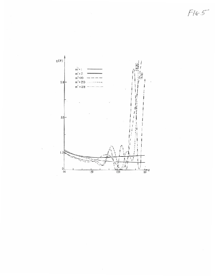
Figure 5: Quantum electron-monopole scattering.

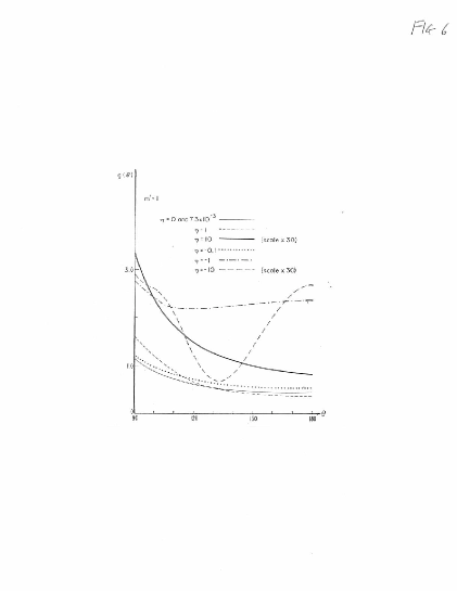
Figure 6: Quantum dyon-dyon scattering, $m^{\prime}=1$.

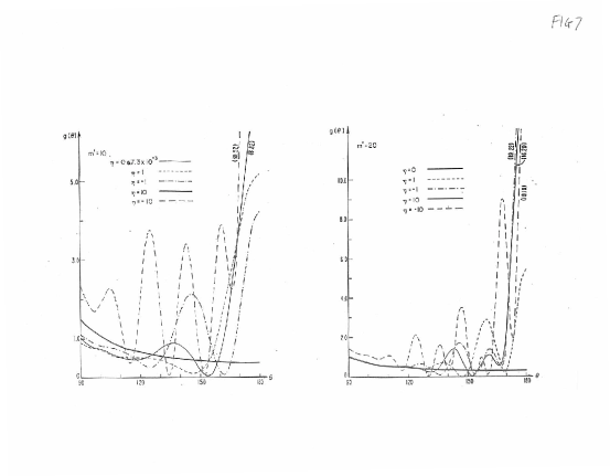
Figure 7: Quantum dyon-dyon scattering, $m^{\prime}=10,20$.

3.2.1 Magnetic dipole interaction

We can also include the effect of a magnetic dipole moment interaction, by adding a spin term to the Hamiltonian,

$$\mathcal{H}_{S}=-\frac{e\hbar}{2\mu c}\gamma\mbox{\boldmath{$\sigma$}}\cdot{\bf B},\qquad{\bf B}=g\frac{{\bf r}}{r^{3}}.$$ (2.2difgknopsacaeanbgbncdcecodgdxdzeg)

For small scattering angles, the spin-flip and spin-nonflip cross sections are for $\gamma=1$ ($\theta\ll 1$)

$$\left.\frac{\rmd\sigma}{\rmd\Omega}\right|_{\rm F}\approx\left(\frac{m^{\prime}}{2k}\right)^{2}\frac{\sin^{2}\theta/2}{\sin^{4}\theta/2},\qquad\left.\frac{\rmd\sigma}{\rmd\Omega}\right|_{\rm NF}\approx\left(\frac{m^{\prime}}{2k}\right)^{2}\frac{\cos^{2}\theta/2}{\sin^{4}\theta/2},$$ (2.2difgknopsacaeanbgbncdcecodgdxdzeh)

Numerical results are shown in figure 8 and figure 9. Note from the figures that the spin flip amplitude always vanishes in the backward direction; the spin nonflip amplitude also vanishes there for conditions almost pertaining to an electron: $m^{\prime}>0$, $\gamma=1$.

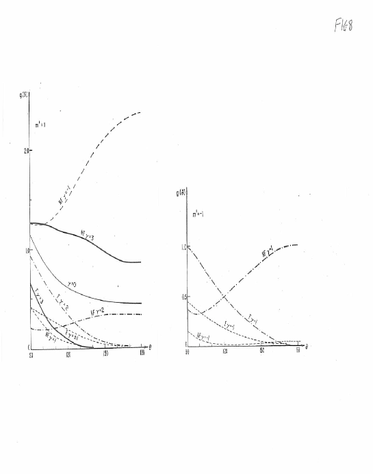
Figure 8: Spinflip (F) and nonflip (NF) cross sections for various gyromagnetic ratios. The first graph shows $m^{\prime}=+1$, the second $m^{\prime}=-1$.

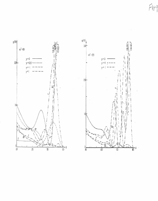
Figure 9: Spinflip and nonflip cross sections for $m^{\prime}=10,20$.

The calculations shown in figures 5–9 were done many years ago [19], which just goes to show that “good work ages more slowly than its creators.” The history of the subject goes much further back. Tamm [54] calculated the wavefunction for the electron-monopole system immediately following Dirac’s suggestion [9]; while Banderet [55], following Fierz [56], was the first to suggest a partial-wave expansion of the scattering amplitude for the system. The first numerical work was carried out by Ford and Wheeler [57], while the comparison with the classical theory can be found, for example, in [58, 59].

3.3 Relativistic calculation

A relativistic calculation of the scattering of a spin-1/2 Dirac particle by a heavy monopole was given by Kazama, Yang, and Goldhaber [39]. They used Yang’s formulation of the vector potential described above in section 3.1.1. In order to arrive a result, they had to add an extra infinitesimal magnetic moment term, in order to prevent the charged particle from passing through the monopole. The sign of this term would have measurable consequences in polarization experiments. It does not, however, appear in the differential cross sections. It also does not affect the helicity flip and helicity nonflip cross sections which are shown in figure 10. The vanishing of the helicity nonflip cross section in the backward direction precisely corresponds to the vanishing of the nonrelativistic spinflip cross section there. The correspondence with the nonrelativistic calculation with spin seems quite close.

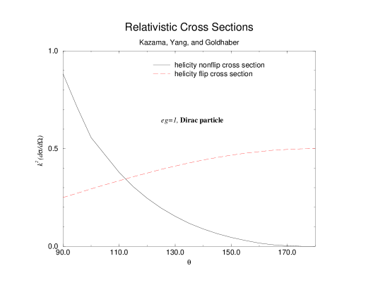
Figure 10: Relativistic helicity-flip and helicity-nonflip cross sections. Note for $\theta=\pi$, helicity nonflip corresponds to spin flip, while helicity flip means spin nonflip.

4 Non-Abelian monopoles

Although the rotationally symmetric, static solution of the Yang-Mills equations was found by Wu and Yang in 1969 [12], it was only in 1974 when ’t Hooft and Polyakov included the Higgs field in the theory that a stable monopole solution was found [13, 14]. Dyonic configurations, that is, ones with both magnetic and arbitrary electric charge, were found by Julia and Zee [16]. Here we discuss the unit monopole solution first obtained by Prasad and Sommerfield [60]. Referred to as BPS monopoles, which saturate the Bogomolny energy bound [61], they are static solutions of the SU(2) theory

$$\mathcal{L}=-\frac{1}{8\pi}\tr(F_{\mu\nu}F^{\mu\nu})+\tr(D_{\mu}HD^{\mu}H)-\frac{1}{4}\lambda\left(2\tr H^{2}-v^{2}\right)^{2}$$

$$=-\frac{1}{16\pi}F_{a}^{\mu\nu}F_{a\mu\nu}+\frac{1}{2}(D_{\mu}H)^{a}(D^{\mu}H)^{2}-\frac{\lambda}{4}(H^{a}H^{a}-v^{2})^{2},$$ (2.2difgknopsacaeanbgbncdcecodgdxdza)

where

$$D_{\mu}H=\partial_{\mu}H-eA_{\mu}\times H,$$ (2.2difgknopsacaeanbgbncdcecodgdxdzb)

for an isotopic triplet Higgs field $H$. (We denote the coupling strength by $e$ to avoid confusion with the magnetic charge $g$.) This is the Georgi-Glashow model [62], in which the massive vector boson has mass

$$m_{W}=\sqrt{4\pi}ev,$$ (2.2difgknopsacaeanbgbncdcecodgdxdzca)

while the Higgs boson mass is

$$m_{H}=\sqrt{\lambda}v.$$ (2.2difgknopsacaeanbgbncdcecodgdxdzcb)

This model possesses nontrivial topological sectors. The topological charge is

$$k=-\frac{e}{16\pi}\int(\rmd\mathbf{x})\epsilon_{ijk}\tr(F_{jk}D_{i}H).$$ (2.2difgknopsacaeanbgbncdcecodgdxdzcd)

In the limit of zero Higgs coupling, $\lambda=0$, where the Higgs boson mass vanishes, Bogomolny showed that the classical energy of the configuration was bounded by the charge,

$$E\geq\sqrt{4\pi}k\frac{v}{e}.$$ (2.2difgknopsacaeanbgbncdcecodgdxdzce)

The solution found by Prasad and Sommerfield achieves the lower bound on the energy, $E=\sqrt{4\pi}kv/e$, with unit charge, $k=1$, and has the form

$$H=\frac{\mathbf{x}}{r}\cdot\boldsymbol{\sigma}h(r),\qquad e\mathbf{A}=\boldsymbol{\sigma}\times\frac{\mathbf{x}}{r^{2}}f(r),$$ (2.2difgknopsacaeanbgbncdcecodgdxdzcfa)

where with $$\xi=\sqrt{4\pi}evr$$

$$h(r)=v\left(\coth\xi-\frac{1}{\xi}\right),\qquad f(r)=1-\frac{\xi}{\sinh\xi},$$ (2.2difgknopsacaeanbgbncdcecodgdxdzcfb)

If we regard $\sigma^{a}/2$ as the isotopic generator, the forms of the isotopic components of the Higgs field and vector potential are

$$H^{a}=2h(r)\frac{x^{a}}{r},\qquad eA^{a}_{i}=2f(r)\epsilon_{aib}\frac{x^{b}}{r^{2}}.$$ (2.2difgknopsacaeanbgbncdcecodgdxdzcfg)

These fields describe a monopole centered on the origin. Far away from that (arbitrary) point, the behavior of the fields is given by

$$r\to\infty:\qquad h(r)\to v,\qquad f(r)\to 1,$$ (2.2difgknopsacaeanbgbncdcecodgdxdzcfh)

so we see that the vector potential (2.2difgknopsacaeanbgbncdcecodgdxdzcfa) indeed describes a monopole of twice the Dirac charge, according to (2.2difgknopsacaeanbgbncdcecodgdj), because the spin is $\mathbf{S}=\frac{1}{2}\boldsymbol{\sigma}$. However, this monopole has structure, and is not singular at the origin, because both $f$ and $h$ vanish there. The energy of the configuration, the mass of the monopole, is finite, as already noted,

$$E=\int(\rmd\mathbf{r})\nabla^{2}\tr H^{2}=\frac{1}{2}\int_{S_{\infty}}\rmd\mathbf{S}\cdot\boldsymbol{\nabla}h^{2}(r)=\sqrt{4\pi}\frac{v^{2}}{ve},$$ (2.2difgknopsacaeanbgbncdcecodgdxdzcfi)

which takes into account the relation between $r$ and $\xi$, as claimed. In physical units this gives a mass of this monopole solution of

$$M=\frac{m_{W}}{\alpha},$$ (2.2difgknopsacaeanbgbncdcecodgdxdzcfj)

in terms of the “fine structure” constant of the gauge coupling, $\alpha=e^{2}$ in Gaussian units. If the electroweak phase transition produced monopoles, then, we would expect them to have a mass of about 10 TeV [63, 64]. There are serious doubts about this possibility [65, 66, 67, 68] so it is far more likely to expect such objects at the GUT scale. Magnetic monopole solutions for gauge theories with arbitrary compact simple gauge groups, as well as noninteracting multimonopole solutions for those theories have been found [69].

In general, the classical ’t Hooft-Polyakov monopole mass in the Georgi-Glashow model is with nonzero Higgs mass is

$$M_{\rm cl}=\frac{m_{W}}{\alpha}\mu(z),\qquad z=\frac{m_{H}}{M_{W}}.$$ (2.2difgknopsacaeanbgbncdcecodgdxdzcfk)

The function $\mu(0)=1$, and is less than 2 for large $z$. Quantum corrections to the classical mass have been considered on the lattice [70].

We will not further discuss non-Abelian monopoles in this review, because that is such a vast subject, and there are many excellent reviews such as [71, 72], as well as textbook discussions [73]. We merely note that asymptotically, an isolated non-Abelian monopole looks just like a Dirac one, so that most of the experimental limits apply equally well to either point-like or solitonic monopoles. Even the difficulties with the Dirac string, which have not been resolved in the second quantized version, to which we now turn our attention, persist with non-Abelian monopoles [74].

5 Quantum field theory

The quantum field theory of magnetic charge has been developed by many people, notably Schwinger [75, 76, 77, 78, 33] and Zwanziger [79, 80, 81, 82]. We should cite the review article by Blagojević and Senjanović [83], which cites earlier work by those authors. A recent formulation suitable for eikonal calculations is given in [84], and will be described in section 5.3 and following.

5.1 Lorentz invariance

Formal Lorentz invariance of the dual quantum electrodynamics system with sources consisting of electric charges $\{e_{a}\}$ and magnetic charges $\{g_{a}\}$ was demonstrated provided the quantization condition holds:

$$e_{a}g_{b}-e_{b}g_{a}=m^{\prime}=\Bigg{\{}\begin{array}[]{l}\frac{n}{2}\,,{\mbox{unsymmetric}}\\ n\,,\mbox{symmetric}\end{array}\Bigg{\}},\qquad n\in\,Z.$$ (2.2difgknopsacaeanbgbncdcecodgdxdzcfc)

“Symmetric” and “unsymmetric” refer to the presence or absence of dual symmetry in the solutions of Maxwell’s equations, reflecting the use of infinite or semi-infinite strings, respectively.

5.2 Quantum action

The electric and magnetic currents are the sources of the field strength and its dual (here, for consistency, we denote by $j^{\mu}$, $\hskip 1.42271pt{}^{\ast}\hskip-1.9919ptj^{\mu}$ what we earlier called $j^{\mu}_{e}$, $j^{\mu}_{m}$, respectively):

$$\partial^{\nu}F_{\mu\nu}=4\pi j_{\mu}\qquad{\mbox{\rm and}}\qquad\partial^{\nu}\hskip 2.84544pt{}^{\ast}F_{\mu\nu}=4\pi\hskip 1.42271pt^{\ast}\hskip-1.9919ptj_{\mu},$$ (2.2difgknopsacaeanbgbncdcecodgdxdzcfd)

where

$$\hskip 2.84544pt{}^{\ast}F_{\mu\nu}=\frac{1}{2}\epsilon_{\mu\nu\sigma\tau}F^{\sigma\tau},$$ (2.2difgknopsacaeanbgbncdcecodgdxdzcfe)

which imply the dual conservation of electric and magnetic currents, $j_{\mu}$ and $\hskip 1.42271pt{}^{\ast}\hskip-1.9919ptj_{\mu}$, respectively,

$$\partial_{\mu}j^{\mu}=0,\qquad\mbox{and}\qquad\partial_{\mu}\hskip 1.42271pt^{\ast}\hskip-1.9919ptj^{\mu}=0.$$ (2.2difgknopsacaeanbgbncdcecodgdxdzcff)

As we will detail below, the relativistic interaction between an electric and a magnetic current is

$$W(j,\hskip 1.42271pt^{\ast}\hskip-1.9919ptj)=\int(\rmd x)(\rmd x^{\prime})(\rmd x^{\prime\prime})\hskip 1.42271pt^{\ast}\hskip-1.9919ptj^{\mu}(x)\epsilon_{\mu\nu\sigma\tau}\partial^{\nu}f^{\sigma}\left(x-x^{\prime}\right)D_{+}\left(x^{\prime}-x^{\prime\prime}\right)j^{\tau}\left(x^{\prime\prime}\right).$$ (2.2difgknopsacaeanbgbncdcecodgdxdzcfg)

Here the electric and magnetic currents are

$$j_{\mu}=e\bar{\psi}\gamma_{\mu}\psi\qquad\mbox{and}\qquad\hskip 1.42271pt^{\ast}\hskip-1.9919ptj_{\mu}=g\bar{\chi}\gamma_{\mu}\chi,$$ (2.2difgknopsacaeanbgbncdcecodgdxdzcfh)

for example, for spin-1/2 particles. The photon propagator is denoted by $D_{+}(x-x^{\prime})$ and $f_{\mu}(x)$ is the Dirac string function which satisfies the differential equation

$$\partial_{\mu}f^{\mu}(x)=4\pi\delta(x),$$ (2.2difgknopsacaeanbgbncdcecodgdxdzcfi)

the four-dimensional generalization of (2.2difgknopq). A formal solution of this equation is given by

$$f^{\mu}(x)=4\pi n^{\mu}\left(n\cdot\partial\right)^{-1}\delta(x),$$ (2.2difgknopsacaeanbgbncdcecodgdxdzcfj)

where $n^{\mu}$ is an arbitrary constant vector. [Equation (2.2difgknopsacaeanbgbncdcecodgdu) results if $\mathbf{\hat{n}=-\hat{z}}$, in which case $\mathbf{f(r},t)=\mathbf{f(r)}\delta(t)$.]

5.3 Field theory of magnetic charge

In order to facilitate the construction of the dual-QED formalism we recognize that the well-known continuous global ${\rm U}(1)$ dual symmetry (2.2b) [75, 78, 33] implied by (2.2difgknopsacaeanbgbncdcecodgdxdzcfd), (2.2difgknopsacaeanbgbncdcecodgdxdzcff), given by

$$\left(\begin{array}[]{c}j^{\prime}\\ {\hskip 1.42271pt{}^{\ast}\hskip-1.9919ptj}^{\prime}\end{array}\right)=\left(\begin{array}[]{cc}\cos\theta&\sin\theta\\ -\sin\theta&\cos\theta\end{array}\right)\left(\begin{array}[]{c}j\\ {\hskip 1.42271pt{}^{\ast}\hskip-1.9919ptj}\end{array}\right),$$ (2.2difgknopsacaeanbgbncdcecodgdxdzcfkg)

$$\left(\begin{array}[]{c}F^{\prime}\\ {\hskip 2.84544pt{}^{\ast}F}^{\prime}\end{array}\right)=\left(\begin{array}[]{cc}\cos\theta&\sin\theta\\ -\sin\theta&\cos\theta\end{array}\right)\left(\begin{array}[]{c}F\\ {\hskip 2.84544pt{}^{\ast}F}\end{array}\right),$$ (2.2difgknopsacaeanbgbncdcecodgdxdzcfkn)

suggests the introduction of an auxiliary vector potential $B_{\mu}(x)$ dual to $A_{\mu}(x)$. In order to satisfy the Maxwell and charge conservation equations, Dirac [85] modified the field strength tensor according to

$$F_{\mu\nu}=\partial_{\mu}A_{\nu}-\partial_{\nu}A_{\mu}+\hskip 2.84544pt^{\ast}G_{\mu\nu},$$ (2.2difgknopsacaeanbgbncdcecodgdxdzcfkl)

where now (2.2difgknopsacaeanbgbncdcecodgdxdzcfd) gives rise to the consistency condition on $G_{\mu\nu}(x)=-G_{\nu\mu}(x)$

$$\partial^{\nu}\ {}^{\ast}F_{\mu\nu}=-\partial^{\nu}G_{\mu\nu}=4\pi{\hskip 1.42271pt{}^{\ast}\hskip-1.9919ptj}_{\mu}.$$ (2.2difgknopsacaeanbgbncdcecodgdxdzcfkm)

We then obtain the following inhomogeneous solution to the dual Maxwell’s equation (2.2difgknopsacaeanbgbncdcecodgdxdzcfkm) for the tensor $G_{\mu\nu}(x)$ in terms of the string function $f_{\mu}$ and the magnetic current $\hskip 1.42271pt{}^{\ast}\hskip-1.9919ptj_{\nu}$:

$$G_{\mu\nu}(x)=4\pi\left(n\cdot\partial\right)^{-1}\left[n_{\mu}\hskip 1.42271pt^{\ast}\hskip-1.9919ptj_{\nu}(x)-n_{\nu}\hskip 1.42271pt^{\ast}\hskip-1.9919ptj_{\mu}(x)\right]$$

$$=\int(\rmd y)\left[f_{\mu}(x-y)\hskip 1.42271pt^{\ast}\hskip-1.9919ptj_{\nu}(y)-f_{\nu}(x-y)\hskip 1.42271pt^{\ast}\hskip-1.9919ptj_{\mu}(y)\right],$$ (2.2difgknopsacaeanbgbncdcecodgdxdzcfkn)

where use is made of (2.2difgknopsacaeanbgbncdcecodgdxdzcff), (2.2difgknopsacaeanbgbncdcecodgdxdzcfi), and (2.2difgknopsacaeanbgbncdcecodgdxdzcfj). A minimal generalization of the QED Lagrangian including electron-monopole interactions reads

$$\mathcal{L}=-\frac{1}{16\pi}F_{\mu\nu}F^{\mu\nu}+\bar{\psi}\left(\rmi\gamma\partial+e\gamma A-m_{\psi}\right)\psi+\bar{\chi}\left(i\gamma\partial-m_{\chi}\right)\chi,$$ (2.2difgknopsacaeanbgbncdcecodgdxdzcfko)

where the coupling of the monopole field $\chi(x)$ to the electromagnetic field occurs through the quadratic field strength term according to (2.2difgknopsacaeanbgbncdcecodgdxdzcfkl). We now rewrite the Lagrangian (2.2difgknopsacaeanbgbncdcecodgdxdzcfko) to display more clearly that interaction by introducing the auxiliary potential $B_{\mu}(x)$.

Variation of (2.2difgknopsacaeanbgbncdcecodgdxdzcfko) with respect to the field variables, $\psi$, $\chi$ and $A_{\mu}$, yields in addition to the Maxwell equations for the field strength, $F_{\mu\nu}$, (2.2difgknopsacaeanbgbncdcecodgdxdzcfd) where $j^{\mu}(x)=e\bar{\psi}(x)\gamma^{\mu}\psi(x)$, the equation of motion for the electron field

$$\left(\rmi\gamma\partial+e\gamma A(x)-m_{\psi}\right)\psi(x)=0,$$ (2.2difgknopsacaeanbgbncdcecodgdxdzcfkp)

and the nonlocal equation of motion for the monopole field,

$$\left(\rmi\gamma\partial-m_{\chi}\right)\chi(x)-\frac{1}{8\pi}\int\left(\rmd y\right)\hskip 2.84544pt^{\ast}F^{\mu\nu}(y)\frac{\delta G_{\mu\nu}(y)}{\delta\bar{\chi}(x)}=0\,.$$ (2.2difgknopsacaeanbgbncdcecodgdxdzcfkq)

[We regard $G_{\mu\nu}(x)$ as dependent on $\bar{\chi}$, $\chi$ but not $A_{\mu}$. Thus, the dual Maxwell equation is given by the subsidiary condition (2.2difgknopsacaeanbgbncdcecodgdxdzcfkm).] It is straightforward to see from the Dirac equation for the monopole (2.2difgknopsacaeanbgbncdcecodgdxdzcfkq) and the construction (2.2difgknopsacaeanbgbncdcecodgdxdzcfkn) that introducing the auxiliary dual field (which is a functional of $F_{\mu\nu}$ and depends on the string function $f_{\mu}$)

$$B_{\mu}(x)=-\frac{1}{4\pi}\int(\rmd y)f^{\nu}\left(x-y\right)\hskip 2.84544pt^{\ast}F_{\mu\nu}(y)\,,$$ (2.2difgknopsacaeanbgbncdcecodgdxdzcfkr)

results in the following Dirac equation for the monopole field

$$\left(\rmi\gamma\partial+g\gamma B(x)-m_{\chi}\right)\chi(x)=0.$$ (2.2difgknopsacaeanbgbncdcecodgdxdzcfks)

Here we have chosen the string to satisfy the oddness condition [this is the “symmetric” solution, generalizing (2.2difgknopsw)]

$$f^{\mu}(x)=-f^{\mu}(-x),$$ (2.2difgknopsacaeanbgbncdcecodgdxdzcfkt)

which as we have seen is related to Schwinger’s integer quantization condition [44, 86]. Now (2.2difgknopsacaeanbgbncdcecodgdxdzcfkp) and (2.2difgknopsacaeanbgbncdcecodgdxdzcfks) display the dual symmetry expressed in Maxwell’s equations (2.2difgknopsacaeanbgbncdcecodgdxdzcfd) and (2.2difgknopsacaeanbgbncdcecodgdxdzcff). Noting that $B_{\mu}$ satisfies [like taking $\lambda_{m}=0$ in (2.2difgknopb)]

$$\int(\rmd x^{\prime})f^{\mu}(x-x^{\prime})B_{\mu}(x^{\prime})=0,$$ (2.2difgknopsacaeanbgbncdcecodgdxdzcfku)

we see that (2.2difgknopsacaeanbgbncdcecodgdxdzcfkr) is a gauge-fixed vector field [87, 88] defined in terms of the field strength through an inversion formula (see section 5.4.1). In terms of these fields the “dual-potential” action can be re-expressed in terms of the vector potential $A_{\mu}$ and field strength tensor $F_{\mu\nu}$ (where $B_{\mu}$ is the functional (2.2difgknopsacaeanbgbncdcecodgdxdzcfkr) of $F_{\mu\nu}$) in first-order formalism as

$$W=\int(\rmd x)\bigg{\{}-\frac{1}{8\pi}F^{\mu\nu}(x)\left(\partial_{\mu}A_{\nu}\left(x\right)-\partial_{\nu}A_{\mu}\left(x\right)\right)+\frac{1}{16\pi}F_{\mu\nu}(x)F^{\mu\nu}(x)$$

$$\mbox{}+\bar{\psi}(x)\left(\rmi\gamma\partial+e{\gamma A}(x)-m_{\psi}\right)\psi(x)+\bar{\chi}(x)\left(\rmi\gamma\partial+g{\gamma B}(x)-m_{\chi}\right)\chi(x)\bigg{\}},$$ (2.2difgknopsacaeanbgbncdcecodgdxdzcfkva)

or in terms of dual variables,

$$W=\int(\rmd x)\bigg{\{}-\frac{1}{8\pi}{\hskip 2.84544pt{}^{\ast}F}^{\mu\nu}(x)\left(\partial_{\mu}B_{\nu}\left(x\right)-\partial_{\nu}B_{\mu}\left(x\right)\right)+\frac{1}{16\pi}{\hskip 2.84544pt{}^{\ast}F}^{\mu\nu}(x){\hskip 2.84544pt{}^{\ast}F}_{\mu\nu}(x)$$

$$\mbox{}+\bar{\psi}(x)\left(\rmi\gamma\partial+e{\gamma A}(x)-m_{\psi}\right)\psi(x)+\bar{\chi}(x)\left(\rmi\gamma\partial+g{\gamma B}(x)-m_{\chi}\right)\chi(x)\bigg{\}}.$$ (2.2difgknopsacaeanbgbncdcecodgdxdzcfkvb)

In (2.2difgknopsacaeanbgbncdcecodgdxdzcfkva), $A_{\mu}(x)$ and $F_{\mu\nu}(x)$ are the independent field variables and $B_{\mu}(x)$ is given by (2.2difgknopsacaeanbgbncdcecodgdxdzcfkr), while in (2.2difgknopsacaeanbgbncdcecodgdxdzcfkvb) the dual fields are the independent variables, in which case,

$$A_{\mu}(x)=-\frac{1}{4\pi}\int(\rmd y)f^{\nu}\left(x-y\right)\ F_{\mu\nu}(y)={1\over 8\pi}\epsilon_{\mu\nu\lambda\sigma}\int(\rmd y)f^{\nu}(x-y)\hskip 2.84544pt^{\ast}F^{\lambda\sigma}(y).$$ (2.2difgknopsacaeanbgbncdcecodgdxdzcfkvw)

[Note that (2.2difgknopsacaeanbgbncdcecodgdxdzcfkvb) may be obtained from the form (2.2difgknopsacaeanbgbncdcecodgdxdzcfkva) by inserting (2.2difgknopsacaeanbgbncdcecodgdxdzcfkvw) into the former and then identifying $B_{\mu}$ according to the construction (2.2difgknopsacaeanbgbncdcecodgdxdzcfkr). In this way the sign of ${1\over 16\pi}F_{\mu\nu}F^{\mu\nu}=-{1\over 16\pi}{}^{*}F_{\mu\nu}{}^{*}F^{\mu\nu}$ is flipped.] Consequently, the field equation relating $\hskip 2.84544pt{}^{\ast}F^{\mu\nu}$ and $B^{\mu}$ is

$${\hskip 2.84544pt{}^{\ast}F}_{\mu\nu}=\partial_{\mu}{B}_{\nu}-\partial_{\nu}{B}_{\mu}-\int(\rmd y)\,{}^{\ast}\left(f_{\mu}(x-y)j_{\nu}(y)-f_{\nu}(x-y)j_{\mu}(y)\right),$$ (2.2difgknopsacaeanbgbncdcecodgdxdzcfkvx)

which is simply obtained (2.2difgknopsacaeanbgbncdcecodgdxdzcfkl) by making the duality transformation (2.2a).

5.4 Quantization of dual QED: Schwinger-Dyson equations

Although the various actions describing the interactions of point electric and magnetic poles can be described in terms of a set of Feynman rules which one conventionally uses in perturbative calculations, the large value of $\alpha_{g}$ or $eg$ renders them useless for this purpose. In addition, calculations of physical processes using the perturbative approach from string-dependent actions such as (2.2difgknopsacaeanbgbncdcecodgdxdzcfkva) and (2.2difgknopsacaeanbgbncdcecodgdxdzcfkvb) have led only to string dependent results [89]. In conjunction with a nonperturbative functional approach, however, the Feynman rules serve to elucidate the electron-monopole interactions. We express these interactions in terms of the “dual-potential” formalism as a quantum generalization of the relativistic classical theory of section 5.3. We use the Schwinger action principle [90, 91] to quantize the electron-monopole system by solving the corresponding Schwinger-Dyson equations for the generating functional. Using a functional Fourier transform of this generating functional in terms of a path integral for the electron-monopole system, we rearrange the generating functional into a form that is well-suited for the purpose of nonperturbative calculations.

5.4.1 Gauge symmetry

In order to construct the generating functional for Green’s functions in the electron-monopole system we must restrict the gauge freedom resulting from the local gauge invariance of the action (2.2difgknopsacaeanbgbncdcecodgdxdzcfkva). The inversion formulae for $A_{\mu}$ and $B_{\mu}$, (2.2difgknopsacaeanbgbncdcecodgdxdzcfkvw) and (2.2difgknopsacaeanbgbncdcecodgdxdzcfkr) respectively, might suggest using the technique of gauge-fixed fields [87, 92] as was adopted in [89]. However, we use the technique of gauge fixing according to methods outlined by Zumino [93, 94] and generalized by Zinn-Justin [95] in the language of stochastic quantization.

The gauge fields are obtained in terms of the string and the gauge invariant field strength, by contracting the field strength (2.2difgknopsacaeanbgbncdcecodgdxdzcfkl), (2.2difgknopsacaeanbgbncdcecodgdxdzcfkn) with the Dirac string, $f^{\mu}(x)$, in conjunction with (2.2difgknopsacaeanbgbncdcecodgdxdzcfi), yielding the following inversion formula for the equation of motion,

$$A_{\mu}(x)=-\frac{1}{4\pi}\int(\rmd x^{\prime})f^{\nu}(x-x^{\prime})F_{\mu\nu}(x^{\prime})+\partial_{\mu}\tilde{\Lambda}_{e}(x),$$ (2.2difgknopsacaeanbgbncdcecodgdxdzcfkvy)

where we use the suggestive notation, ${\tilde{\Lambda}}_{e}(x)$

$$\tilde{\Lambda}_{e}(x)=\frac{1}{4\pi}\int(\rmd x^{\prime})f^{\nu}(x-x^{\prime})A_{\nu}\left(x^{\prime}\right).$$ (2.2difgknopsacaeanbgbncdcecodgdxdzcfkvz)

In a similar manner, given the dual field strength (2.2difgknopsacaeanbgbncdcecodgdxdzcfkvx) the dual vector potential takes the following form [cf. (2.2difgknopsacaeanbgbncdcecodgdxdzcfkr), (2.2difgknopsacaeanbgbncdcecodgdxdzcfku)]

$$B_{\mu}(x)=-\frac{1}{4\pi}\int(\rmd x^{\prime})f^{\nu}(x-x^{\prime}){\hskip 2.84544pt{}^{\ast}F}_{\mu\nu}(x^{\prime})+\partial_{\mu}\tilde{\Lambda}_{g},$$ (2.2difgknopsacaeanbgbncdcecodgdxdzcfkvaaa)

where

$$\tilde{\Lambda}_{g}(x)=\frac{1}{4\pi}\int(\rmd x^{\prime})f^{\mu}(x-x^{\prime})B_{\mu}(x^{\prime}).$$ (2.2difgknopsacaeanbgbncdcecodgdxdzcfkvaab)

It is evident that (2.2difgknopsacaeanbgbncdcecodgdxdzcfkvy) transforms consistently under a gauge transformation

$$A_{\nu}(x)\longrightarrow A_{\nu}(x)+\partial_{\nu}\Lambda_{e}(x),$$ (2.2difgknopsacaeanbgbncdcecodgdxdzcfkvaaab)

while in addition we note that the Lagrangian (2.2difgknopsacaeanbgbncdcecodgdxdzcfkva) is invariant under the gauge transformation,

$$\psi\rightarrow{\exp}\left[\rmi e\Lambda_{e}\right]\psi,\qquad A_{\mu}\rightarrow A_{\mu}+\partial_{\mu}\Lambda_{e},$$ (2.2difgknopsacaeanbgbncdcecodgdxdzcfkvaaaca)

as is the dual action (2.2difgknopsacaeanbgbncdcecodgdxdzcfkvb) under

$$\chi\rightarrow{\rm exp}\left[\rmi g\Lambda_{g}\right]\chi,\qquad B_{\mu}\rightarrow B_{\mu}+\partial_{\mu}\Lambda_{g}.$$ (2.2difgknopsacaeanbgbncdcecodgdxdzcfkvaaacb)

Assuming the freedom to choose $\tilde{\Lambda}_{e}(x)=-\Lambda_{e}(x)$, we bring the vector potential into gauge-fixed form, coinciding with (2.2difgknopsacaeanbgbncdcecodgdxdzcfkvw),

$$A_{\mu}(x)=-\frac{1}{4\pi}\int(\rmd y)f^{\nu}\left(x-y\right)\ F_{\mu\nu}(y)$$ (2.2difgknopsacaeanbgbncdcecodgdxdzcfkvaaacad)

where the gauge choice is equivalent to a string-gauge condition

$$\int\ (\rmd x^{\prime})f^{\mu}(x-x^{\prime})A_{\mu}(x^{\prime})=0.$$ (2.2difgknopsacaeanbgbncdcecodgdxdzcfkvaaacae)

[This is the analog of (2.2difgknopsacaeanbgbncdcecodgdxdzcfku), and is equivalent to the gauge choice $\lambda_{e}=0$, see (2.2difgknopa), used in section 3.1.3. It is worth noting the similarity of this condition to the Schwinger-Fock gauge in ordinary QED, $x\cdot{\cal A}(x)=0$ which yields the gauge-fixed photon field, ${\cal A}_{\mu}(x)=-x^{\nu}\int_{0}^{1}ds\,sF_{\mu\nu}(xs)$.] Taking the divergence of (2.2difgknopsacaeanbgbncdcecodgdxdzcfkvaaacad) and using (2.2difgknopsacaeanbgbncdcecodgdxdzcfd), the gauge-fixed condition (2.2difgknopsacaeanbgbncdcecodgdxdzcfkvaaacad) can be written as

$$\partial_{\mu}A^{\mu}=\int(\rmd y)f^{\mu}\left(x-y\right)j_{\mu}(y),$$ (2.2difgknopsacaeanbgbncdcecodgdxdzcfkvaaacaf)

which is nothing other than the gauge-fixed condition of Zwanziger in the two-potential formalism [80].

More generally, the fact that a gauge function exists, such that ${\Lambda}_{e}(x)=-\tilde{\Lambda}_{e}(x)$ [cf. (2.2difgknopsacaeanbgbncdcecodgdxdzcfkvz)], implying that we have the freedom to consistently fix the gauge, is in fact not a trivial claim. If this were not true, it would certainly derail the consistency of incorporating monopoles into QED while utilizing the Dirac string formalism. On the contrary, the string-gauge condition (2.2difgknopsacaeanbgbncdcecodgdxdzcfkvaaacae) is in fact a class of possible consistent gauge conditions characterized by the symbolic operator function (2.2difgknopsacaeanbgbncdcecodgdxdzcfj) depending on a unit vector $n^{\mu}$ (which may be either spacelike or timelike).

In order to quantize this system we must divide out the equivalence class of field values defined by a gauge trajectory in field space; in this sense the gauge condition restricts the vector potential to a hypersurface of field space which is embodied in the generalization of (2.2difgknopsacaeanbgbncdcecodgdxdzcfkvaaacae)

$$\frac{1}{4\pi}\int(\rmd x^{\prime})f^{\mu}(x-x^{\prime})A_{\mu}(x^{\prime})=\Lambda^{f}_{e}(x),$$ (2.2difgknopsacaeanbgbncdcecodgdxdzcfkvaaacag)

where here $\Lambda^{f}_{e}$ is any function defining a unique gauge fixing hypersurface in field space.

In a path integral formalism, we enforce the condition (2.2difgknopsacaeanbgbncdcecodgdxdzcfkvaaacag) by introducing a $\delta$ function, symbolically written as

$$\delta\left(\frac{1}{4\pi}f^{\mu}A_{\mu}-\Lambda^{f}_{e}\right)=\int[\rmd\lambda_{e}]\exp\Bigg{[}\rmi\int(\rmd x)\lambda_{e}(x)$$

$$\times\left(\frac{1}{4\pi}\int(\rmd x^{\prime})f^{\mu}(x-x^{\prime})A_{\mu}(x^{\prime})-\Lambda^{f}_{e}(x)\right)\Bigg{]},$$ (2.2difgknopsacaeanbgbncdcecodgdxdzcfkvaaacah)

or by introducing a Gaussian functional integral

$$\Phi\left(\frac{1}{4\pi}f^{\mu}A_{\mu}-\Lambda^{f}_{e}\right)=\int[\rmd\lambda_{e}]\exp\Bigg{[}-\frac{\rmi}{2}\int(\rmd x)(\rmd x^{\prime})\lambda_{e}(x)M(x,x^{\prime})\lambda_{e}(x^{\prime})$$

$$\mbox{}+\rmi\int(\rmd x)\lambda_{e}(x)\left(\frac{1}{4\pi}\int(\rmd x^{\prime})f^{\mu}(x-x^{\prime})A_{\mu}(x^{\prime})-\Lambda^{f}_{e}(x)\right)\Bigg{]},$$ (2.2difgknopsacaeanbgbncdcecodgdxdzcfkvaaacai)

where the symmetric matrix $M(x,x^{\prime})=\kappa^{-1}\delta(x-x^{\prime})$ describes the spread of the integral $\int(\rmd x^{\prime})f^{\mu}(x-x^{\prime})A_{\mu}(x^{\prime})$ about the gauge function, $\Lambda^{f}_{e}(x)$. That is, we enforce the gauge fixing condition (2.2difgknopsacaeanbgbncdcecodgdxdzcfkvaaacag) by adding the quadratic form appearing here to the action (2.2difgknopsacaeanbgbncdcecodgdxdzcfkva) and in turn eliminating $\lambda_{e}$ by its “equation of motion”

$$\lambda_{e}(x)=\kappa\left(\frac{1}{4\pi}\int(\rmd y)\,f^{\mu}(x-y)A_{\mu}(y)-\Lambda^{f}_{e}(x)\right).$$ (2.2difgknopsacaeanbgbncdcecodgdxdzcfkvaaacaj)

Now the equations of motion (2.2difgknopsacaeanbgbncdcecodgdxdzcfd) take the form,

$$\partial^{\nu}F_{\mu\nu}(x)-\int(\rmd x^{\prime})\lambda_{e}(x^{\prime})f_{\mu}(x^{\prime}-x)=4\pi j_{\mu}(x),$$ (2.2difgknopsacaeanbgbncdcecodgdxdzcfkvaaacaka)

$$\partial^{\nu}\hskip 2.84544pt{}^{\ast}F_{\mu\nu}(x)-\int(\rmd x^{\prime})\lambda_{g}(x^{\prime})f_{\mu}(x^{\prime}-x)=4\pi\hskip 1.42271pt^{\ast}\hskip-1.9919ptj_{\mu}(x),$$ (2.2difgknopsacaeanbgbncdcecodgdxdzcfkvaaacakb)

where the second equation refers to a similar gauge fixing in the dual sector. Taking the divergence of (2.2difgknopsacaeanbgbncdcecodgdxdzcfkvaaacaka) implies $\lambda_{e}=0$ from (2.2difgknopsacaeanbgbncdcecodgdxdzcfi) and (2.2difgknopsacaeanbgbncdcecodgdxdzcff), which consistently yields the gauge condition (2.2difgknopsacaeanbgbncdcecodgdxdzcfkvaaacag). Using our freedom to make a transformation to the gauge-fixed condition (2.2difgknopsacaeanbgbncdcecodgdxdzcfkvaaacad), $\Lambda^{f}_{e}=0$, the equation of motion (2.2difgknopsacaeanbgbncdcecodgdxdzcfkvaaacaka) for the potential becomes

$$\Bigg{[}-g_{\mu\nu}\partial^{2}+\partial_{\mu}\partial_{\nu}+4\pi\kappa n_{\mu}(n\cdot\partial)^{-2}n_{\nu}\Bigg{]}A^{\nu}(x)=4\pi j_{\mu}(x)+\epsilon_{\mu\nu\sigma\tau}\frac{4\pi n^{\nu}}{\left(n\cdot\partial\right)}\partial^{\sigma}\hskip 1.42271pt{}^{\ast}\hskip-1.9919ptj^{\tau}(x),$$ (2.2difgknopsacaeanbgbncdcecodgdxdzcfkvaaacakal)

where we now have used the symbolic form of the string function (2.2difgknopsacaeanbgbncdcecodgdxdzcfj). Even though (2.2difgknopsacaeanbgbncdcecodgdxdzcfkvaaacaj) now implies $n^{\mu}A_{\mu}=0$, we have retained the term proportional to $n_{\mu}n_{\nu}$ in the kernel, scaled by the arbitrary parameter $\kappa$,

$$K_{\mu\nu}=\Bigg{[}-g_{\mu\nu}\partial^{2}+\partial_{\mu}\partial_{\nu}+4\pi\kappa\,n_{\mu}(n\cdot\partial)^{-2}n_{\nu}\Bigg{]},$$ (2.2difgknopsacaeanbgbncdcecodgdxdzcfkvaaacakam)

so that $K_{\mu\nu}$ possesses an inverse

$$D_{\mu\nu}(x)=\Bigg{[}g_{\mu\nu}-\frac{n_{\mu}\partial_{\nu}+n_{\nu}\partial_{\mu}}{(n\cdot\partial)}+n^{2}\left(1-\frac{1}{4\pi\kappa}\frac{(n\cdot\partial)^{2}\partial^{2}}{n^{2}}\right)\frac{\partial_{\mu}\partial_{\nu}}{(n\cdot\partial)^{2}}\Bigg{]}D_{+}(x),$$ (2.2difgknopsacaeanbgbncdcecodgdxdzcfkvaaacakan)

that is, $\int(\rmd x^{\prime})K_{\mu\alpha}(x-x^{\prime})D^{\alpha\nu}(x^{\prime}-x^{\prime\prime})=g_{\mu}^{\nu}\delta(x-x^{\prime\prime})$, where $D_{+}(x)$ is the massless scalar propagator,

$$D_{+}(x)=\frac{1}{-\partial^{2}-\rmi\epsilon}\delta(x).$$ (2.2difgknopsacaeanbgbncdcecodgdxdzcfkvaaacakao)

This in turn enables us to rewrite (2.2difgknopsacaeanbgbncdcecodgdxdzcfkvaaacakal) as an integral equation, expressing the vector potential in terms of the electron and monopole currents,

$$A_{\mu}(x)=4\pi\int(\rmd x^{\prime})D_{\mu\nu}(x-x^{\prime})j^{\nu}(x^{\prime})$$

$$\mbox{}+\epsilon^{\nu\lambda\sigma\tau}\int(\rmd x^{\prime})(\rmd x^{\prime\prime})D_{\mu\nu}(x-x^{\prime})f_{\lambda}(x^{\prime}-x^{\prime\prime})\partial^{\prime\prime}_{\sigma}\hskip 1.42271pt{}^{\ast}\hskip-1.9919ptj_{\tau}(x^{\prime\prime}).$$ (2.2difgknopsacaeanbgbncdcecodgdxdzcfkvaaacakap)

The steps for $B_{\mu}(x)$ are analogous.

5.4.2 Vacuum persistence amplitude and the path integral

Given the gauge-fixed but string-dependent action, we are prepared to quantize this theory of dual QED. Quantization using a path integral formulation of such a string-dependent action is by no means straightforward; therefore we will develop the generating functional making use of a functional approach. Using the quantum action principle (cf. [90, 91]) we write the generating functional for Green’s functions (or the vacuum persistence amplitude) in the presence of external sources ${\cal K}$,

$$Z({\cal K})=\langle 0_{+}\left|\right.0_{-}\rangle^{\cal K},$$ (2.2difgknopsacaeanbgbncdcecodgdxdzcfkvaaacakaq)

for the electron-monopole system. Schwinger’s action principle states that under an arbitrary variation

$$\delta\langle 0_{+}\left|\right.0_{-}\rangle^{{\cal K}}=\rmi\langle 0_{+}\left|\delta W({\cal K})\right|0_{-}\rangle^{{\cal K}}\,,$$ (2.2difgknopsacaeanbgbncdcecodgdxdzcfkvaaacakar)

where $W({\cal K})$ is the action given in (2.2difgknopsacaeanbgbncdcecodgdxdzcfkva) externally driven by the sources, ${\cal K}$, which for the present case are given by the set $\{J,\hskip 1.42271pt^{\ast}\hskip-1.9919ptJ,\bar{\eta},\eta,\bar{\xi},\xi\}$:

$$W({\cal K})=W+\int(\rmd x)\left\{J^{\mu}A_{\mu}+{}^{*}J^{\mu}B_{\mu}+\bar{\eta}\psi+\bar{\psi}\eta+\bar{\xi}\chi+\bar{\chi}\xi\right\},$$ (2.2difgknopsacaeanbgbncdcecodgdxdzcfkvaaacakas)

$\eta$ ($\bar{\eta}$), $\xi$ ($\bar{\xi}$) being the sources for electrons (positrons) and monopoles (antimonopoles), respectively. The one-point functions are then given by

$$\frac{\delta}{\rmi\delta J^{\mu}(x)}\log Z({\cal K})=\frac{\langle 0_{+}|A_{\mu}(x)|0_{-}\rangle^{\cal K}}{\langle 0_{+}\left|\right.0_{-}\rangle^{\cal K}},\qquad\frac{\delta}{\rmi\delta\hskip 1.42271pt^{\ast}\hskip-1.9919ptJ^{\mu}(x)}\log Z({\cal K})=\frac{\langle 0_{+}|B_{\mu}(x)|0_{-}\rangle^{\cal K}}{\langle 0_{+}\left|\right.0_{-}\rangle^{\cal K}},$$

$$\frac{\delta}{\rmi\delta\bar{\eta}(x)}\log Z({\cal K})=\frac{\langle 0_{+}|\psi(x)|0_{-}\rangle^{\cal K}}{\langle 0_{+}\left|\right.0_{-}\rangle^{\cal K}},\qquad\frac{\delta}{\rmi\delta\bar{\xi}(x)}\log Z({\cal K})=\frac{\langle 0_{+}|\chi(x)|0_{-}\rangle^{\cal K}}{\langle 0_{+}\left|\right.0_{-}\rangle^{\cal K}}.$$ (2.2difgknopsacaeanbgbncdcecodgdxdzcfkvaaacakat)

Using (2.2difgknopsacaeanbgbncdcecodgdxdzcfkvaaacakat) we can write down derivatives with respect to the charges (here we redefine the electric and magnetic currents $j\rightarrow ej$ and $\hskip 1.42271pt{}^{\ast}\hskip-1.9919ptj\rightarrow g\hskip 1.42271pt^{\ast}\hskip-1.9919ptj$) in terms of functional derivatives [96, 97, 98] with respect to the external sources;

$$\frac{\partial}{\partial e}\langle 0_{+}|0_{-}\rangle^{{\cal K}}=\rmi\langle 0_{+}\big{|}\int(\rmd x)j^{\mu}(x)A_{\mu}(x)\big{|}0_{-}\rangle^{{\cal K}}=-\rmi\int(\rmd x)\left(\frac{\delta}{\delta\tilde{A}_{\mu}(x)}\frac{\delta}{\delta J^{\mu}(x)}\right)\langle 0_{+}\big{|}0_{-}\rangle^{{\cal K}},$$

$$\frac{\partial}{\partial g}\langle 0_{+}|0_{-}\rangle^{{\cal K}}=\rmi\langle 0_{+}\big{|}\int(\rmd x)\hskip 1.42271pt^{\ast}\hskip-1.9919ptj^{\mu}(x)B_{\mu}(x)\big{|}0_{-}\rangle^{{\cal K}}=-\rmi\int(\rmd x)\left(\frac{\delta}{\delta\tilde{B}_{\mu}(x)}\frac{\delta}{\delta\hskip 1.42271pt^{\ast}\hskip-1.9919ptJ^{\mu}(x)}\right)\langle 0_{+}\big{|}0_{-}\rangle^{{\cal K}}.$$

Here we have introduced an effective source to bring down the electron and monopole currents,

$${\delta\over\delta\tilde{A}_{\mu}}\equiv{1\over\rmi}{\delta\over\delta\eta}\gamma^{\mu}{\delta\over\delta\bar{\eta}},\qquad{\delta\over\delta\tilde{B}_{\mu}}\equiv{1\over\rmi}{\delta\over\delta\xi}\gamma^{\mu}{\delta\over\delta\bar{\xi}}.$$ (2.2difgknopsacaeanbgbncdcecodgdxdzcfkvaaacakav)

These first order differential equations can be integrated with the result

$$\langle 0_{+}\left|\right.0_{-}\rangle^{{\cal K}}=\exp\Bigg{[}-\rmi g\int(\rmd x)\left(\frac{\delta}{\delta\tilde{B}_{\nu}(x)}\frac{\delta}{\delta\hskip 1.42271pt^{\ast}\hskip-1.9919ptJ^{\nu}(x)}\right)$$

$$-\rmi e\int(\rmd x)\left(\frac{\delta}{\delta\tilde{A}_{\mu}(x)}\frac{\delta}{\delta J^{\mu}(x)}\right)\Bigg{]}\langle 0_{+}\left|\right.0_{-}\rangle^{{\cal K}}_{0},$$ (2.2difgknopsacaeanbgbncdcecodgdxdzcfkvaaacakaw)

where $\langle 0_{+}\left|\right.0_{-}\rangle^{{\cal K}}_{0}$ is the vacuum amplitude in the absence of interactions. By construction, the vacuum amplitude and Green’s functions for the coupled problem are determined by functional derivatives with respect to the external sources ${\cal K}$ of the uncoupled vacuum amplitude, where $\langle 0_{+}\left|\right.0_{-}\rangle^{{\cal K}}_{0}$ is the product of the separate amplitudes for the quantized electromagnetic and Dirac fields since they constitute completely independent systems in the absence of coupling, that is,

$$\langle 0_{+}\left|\right.0_{-}\rangle^{{\cal K}}_{0}=\langle 0_{+}\left|\right.0_{-}\rangle^{(\bar{\eta},\eta,\bar{\xi},\xi)}_{0}\langle 0_{+}\left|\right.0_{-}\rangle^{(J,\hskip 1.42271pt^{\ast}\hskip-1.9919ptJ)}_{0}.$$ (2.2difgknopsacaeanbgbncdcecodgdxdzcfkvaaacakax)

First we consider $\langle 0_{+}\left|\right.0_{-}\rangle^{{\cal K}}_{0}$ as a function of $J$ and $\hskip 1.42271pt{}^{\ast}\hskip-1.9919ptJ$

$$\frac{\delta}{\rmi\delta J^{\mu}(x)}\langle 0_{+}\left|\right.0_{-}\rangle^{\cal K}_{0}=\langle 0_{+}|A_{\mu}(x)|0_{-}\rangle^{\cal K}_{0}.$$ (2.2difgknopsacaeanbgbncdcecodgdxdzcfkvaaacakay)

Taking the matrix element of the integral equation (2.2difgknopsacaeanbgbncdcecodgdxdzcfkvaaacakap) but now with external sources rather than dynamical currents we find

$$\langle 0_{+}|A_{\mu}(x)|0_{-}\rangle^{\cal K}_{0}=\int(\rmd x^{\prime})D_{\mu\nu}(x-x^{\prime})\left(4\pi J^{\nu}(x^{\prime})+\epsilon^{\nu\lambda\sigma\tau}\int(\rmd x^{\prime\prime})f_{\lambda}(x^{\prime}-x^{\prime\prime})\partial^{\prime\prime}_{\sigma}\hskip 1.42271pt{}^{\ast}\hskip-1.9919ptJ_{\tau}(x^{\prime\prime})\right)$$

$$\times\langle 0_{+}|0_{-}\rangle_{0}^{\cal K}.$$ (2.2difgknopsacaeanbgbncdcecodgdxdzcfkvaaacakaz)

Using (2.2difgknopsacaeanbgbncdcecodgdxdzcfkvaaacakal) we arrive at the equivalent gauge-fixed functional equation,

$$\Bigg{[}-g_{\mu\nu}\partial^{2}+\partial_{\mu}\partial_{\nu}+4\pi\kappa n_{\mu}(n\cdot\partial)^{-2}n_{\nu}\Bigg{]}\frac{\delta}{\rmi\delta J^{\nu}(x)}\langle 0_{+}\left|\right.0_{-}\rangle^{{\cal K}}_{0}$$

$$=\left(4\pi J_{\mu}(x)+\epsilon_{\mu\nu\sigma\tau}\int(\rmd x^{\prime})f^{\nu}(x-x^{\prime})\partial^{\prime\sigma}\hskip 1.42271pt{}^{\ast}\hskip-1.9919ptJ^{\tau}(x^{\prime})\right)\langle 0_{+}\left|\right.0_{-}\rangle^{{\cal K}}_{0},$$ (2.2difgknopsacaeanbgbncdcecodgdxdzcfkvaaacakba)

which is subject to the gauge condition

$$n^{\nu}{\delta\over\delta J^{\nu}}\langle 0_{+}|0_{-}\rangle_{0}^{\cal K}=0,$$ (2.2difgknopsacaeanbgbncdcecodgdxdzcfkvaaacakbba)

or

$$\int(\rmd x^{\prime})f^{\nu}(x-x^{\prime}){\delta\over\delta J^{\nu}(x^{\prime})}\langle 0_{+}|0_{-}\rangle_{0}^{\cal K}=0.$$ (2.2difgknopsacaeanbgbncdcecodgdxdzcfkvaaacakbbb)

In turn, from (2.2difgknopsacaeanbgbncdcecodgdxdzcfkvaaacakaw) we obtain the full functional equation for $\langle 0_{+}\left|\right.0_{-}\rangle^{{\cal K}}$:

$$\Bigg{[}-g_{\mu\nu}\partial^{2}+\partial_{\mu}\partial_{\nu}+4\pi\kappa n_{\mu}(n\cdot\partial)^{-2}n_{\nu}\Bigg{]}\frac{\delta}{\rmi\delta J^{\nu}(x)}\langle 0_{+}\left|\right.0_{-}\rangle^{{\cal K}}$$

$$=\exp\left[-\rmi g\int(\rmd y)\left(\frac{\delta}{\delta\tilde{B}_{\alpha}(y)}\frac{\delta}{\delta\hskip 1.42271pt^{\ast}\hskip-1.9919ptJ^{\alpha}(y)}\right)-\rmi e\int(\rmd y)\left(\frac{\delta}{\delta\tilde{A}_{\alpha}(y)}\frac{\delta}{\delta J^{\alpha}(y)}\right)\right]$$

$$\times\left(4\pi J_{\mu}(x)+\epsilon_{\mu\nu\sigma\tau}\int(\rmd x^{\prime})f^{\nu}(x-x^{\prime})\partial^{\prime\sigma}\hskip 1.42271pt{}^{\ast}\hskip-1.9919ptJ^{\tau}(x^{\prime})\right)\langle 0_{+}\left|\right.0_{-}\rangle^{{\cal K}}_{0}.$$ (2.2difgknopsacaeanbgbncdcecodgdxdzcfkvaaacakbbbc)

Commuting the external currents to the left of the exponential on the right side of (2.2difgknopsacaeanbgbncdcecodgdxdzcfkvaaacakbbbc) and using (2.2difgknopsacaeanbgbncdcecodgdxdzcfkvaaacakat), we are led to the Schwinger-Dyson equation for the vacuum amplitude, where we have restored the meaning of the functional derivatives with respect to $\tilde{A}$, $\tilde{B}$ given in (2.2difgknopsacaeanbgbncdcecodgdxdzcfkvaaacakav),

$$\Bigg{\{}\bigg{[}-g_{\mu\nu}\partial^{2}+\partial_{\mu}\partial_{\nu}+4\pi\kappa n_{\mu}(n\cdot\partial)^{-2}n_{\nu}\bigg{]}\frac{\delta}{\rmi\delta J_{\nu}(x)}$$

$$\mbox{}-4\pi e\frac{\delta}{\rmi\delta\eta(x)}\gamma_{\mu}\frac{\delta}{\rmi\delta\bar{\eta}(x)}-\epsilon_{\mu\nu\sigma\tau}\int(\rmd x^{\prime})f^{\nu}(x-x^{\prime})\partial^{\prime\sigma}g\frac{\delta}{\rmi\delta\xi(x^{\prime})}\gamma^{\tau}\frac{\delta}{\rmi\delta\bar{\xi}(x^{\prime})}\Bigg{\}}\langle 0_{+}\left|\right.0_{-}\rangle^{{\cal K}}$$

$$=\left(4\pi J_{\mu}(x)+\epsilon_{\mu\nu\sigma\tau}\int(\rmd x^{\prime})f^{\nu}(x-x^{\prime})\partial^{\prime\sigma}\hskip 1.42271pt{}^{\ast}\hskip-1.9919ptJ^{\tau}(x^{\prime})\right)\langle 0_{+}\left|\right.0_{-}\rangle^{{\cal K}}.$$ (2.2difgknopsacaeanbgbncdcecodgdxdzcfkvaaacakbbbd)

In an analogous manner, using

$$\frac{\delta}{\rmi\delta\hskip 1.42271pt^{\ast}\hskip-1.9919ptJ^{\mu}(x)}\langle 0_{+}\left|\right.0_{-}\rangle^{\cal K}_{0}=\langle 0_{+}|B_{\mu}(x)|0_{-}\rangle^{\cal K}_{0},$$ (2.2difgknopsacaeanbgbncdcecodgdxdzcfkvaaacakbbbe)

we obtain the functional equation (which is consistent with duality)

$$\Bigg{\{}\bigg{[}-g_{\mu\nu}\partial^{2}+\partial_{\mu}\partial_{\nu}+4\pi\kappa n_{\mu}(n\cdot\partial)^{-2}n_{\nu}\bigg{]}\frac{\delta}{\rmi\delta\hskip 1.42271pt^{\ast}\hskip-1.9919ptJ_{\nu}(x)}$$

$$\mbox{}-4\pi g\frac{\delta}{\rmi\delta\xi(x)}\gamma_{\mu}\frac{\delta}{\rmi\delta\bar{\xi}(x)}+\epsilon_{\mu\nu\sigma\tau}\int(\rmd x^{\prime})f^{\nu}(x-x^{\prime})\partial^{\prime\sigma}e\frac{\delta}{\rmi\delta\eta(x^{\prime})}\gamma^{\tau}\frac{\delta}{\rmi\delta\bar{\eta}(x^{\prime})}\Bigg{\}}\langle 0_{+}\left|\right.0_{-}\rangle^{{\cal K}}$$

$$=\left(4\pi\hskip 1.42271pt^{\ast}\hskip-1.9919ptJ_{\mu}(x)-\epsilon_{\mu\nu\sigma\tau}\int(\rmd x^{\prime})f^{\nu}(x-x^{\prime})\partial^{\prime\sigma}J^{\tau}(x^{\prime})\right)\langle 0_{+}\left|\right.0_{-}\rangle^{{\cal K}},$$ (2.2difgknopsacaeanbgbncdcecodgdxdzcfkvaaacakbbbf)

which is subject to the gauge condition

$$\int(\rmd x^{\prime})f^{\mu}(x-x^{\prime}){\delta\over\delta\hskip 1.42271pt^{\ast}\hskip-1.9919ptJ^{\mu}(x^{\prime})}\langle 0_{+}|0_{-}\rangle^{\cal K}=0.$$ (2.2difgknopsacaeanbgbncdcecodgdxdzcfkvaaacakbbbg)

In a straightforward manner we obtain the functional Dirac equations

$$\left\{\rmi\gamma\partial+e\gamma^{\mu}\frac{\delta}{\rmi\delta J^{\mu}(x)}-m_{\psi}\right\}\frac{\delta}{\rmi\delta\bar{\eta}(x)}\langle 0_{+}\left|\right.0_{-}\rangle^{{\cal K}}=-\eta(x)\langle 0_{+}\left|\right.0_{-}\rangle^{{\cal K}},$$ (2.2difgknopsacaeanbgbncdcecodgdxdzcfkvaaacakbbbha)

$$\left\{\rmi\gamma\partial+g\gamma^{\mu}\frac{\delta}{\rmi\delta\hskip 1.42271pt^{\ast}\hskip-1.9919ptJ^{\mu}(x)}-m_{\chi}\right\}\frac{\delta}{\rmi\delta\bar{\xi}(x)}\langle 0_{+}\left|\right.0_{-}\rangle^{{\cal K}}=-\xi(x)\langle 0_{+}\left|\right.0_{-}\rangle^{{\cal K}}.$$ (2.2difgknopsacaeanbgbncdcecodgdxdzcfkvaaacakbbbhb)

In order to obtain a generating functional for Green’s functions we must solve the set of equations (2.2difgknopsacaeanbgbncdcecodgdxdzcfkvaaacakbbbd), (2.2difgknopsacaeanbgbncdcecodgdxdzcfkvaaacakbbbf), (2.2difgknopsacaeanbgbncdcecodgdxdzcfkvaaacakbbbha), (2.2difgknopsacaeanbgbncdcecodgdxdzcfkvaaacakbbbhb) subject to (2.2difgknopsacaeanbgbncdcecodgdxdzcfkvaaacakbbb) and (2.2difgknopsacaeanbgbncdcecodgdxdzcfkvaaacakbbbg) for $\langle 0_{+}\left|\right.0_{-}\rangle^{{\cal J}}$. In the absence of interactions, we can immediately integrate the Schwinger-Dyson equations; in particular, (2.2difgknopsacaeanbgbncdcecodgdxdzcfkvaaacakbbbf) then integrates to

$$\langle 0_{+}\left|\right.0_{-}\rangle^{J,\hskip 1.42271pt^{\ast}\hskip-1.9919ptJ}_{0}={\cal N}(J)\exp\bigg{\{}2\pi\rmi\int(\rmd x)(\rmd x^{\prime})\hskip 1.42271pt^{\ast}\hskip-1.9919ptJ_{\mu}\left(x\right)D^{\mu\nu}(x-x^{\prime})\hskip 1.42271pt^{\ast}\hskip-1.9919ptJ_{\nu}(x^{\prime})$$

$$\mbox{}+\rmi\epsilon_{\mu\nu\sigma\tau}\int(\rmd x)(\rmd x^{\prime})(\rmd x^{\prime\prime})\hskip 1.42271pt^{\ast}\hskip-1.9919ptJ_{\beta}(x)D^{\beta\mu}(x-x^{\prime})\partial^{\prime\nu}f^{\sigma}(x^{\prime}-x^{\prime\prime})J^{\tau}(x^{\prime\prime})\bigg{\}}.$$ (2.2difgknopsacaeanbgbncdcecodgdxdzcfkvaaacakbbbhbi)

We determine ${\cal N}$, which depends only on $J$, by inserting (2.2difgknopsacaeanbgbncdcecodgdxdzcfkvaaacakbbbhbi) into (2.2difgknopsacaeanbgbncdcecodgdxdzcfkvaaacakbbbd) or (2.2difgknopsacaeanbgbncdcecodgdxdzcfkvaaacakba):

$$\ln{\cal N}(J)=2\pi\rmi\int(\rmd x)(\rmd x^{\prime})J_{\mu}(x)D^{\mu\nu}(x-x^{\prime})J_{\nu}(x^{\prime}),$$ (2.2difgknopsacaeanbgbncdcecodgdxdzcfkvaaacakbbbhbj)

resulting in the generating functional for the photonic sector

$$\langle 0_{+}\left|\right.0_{-}\rangle^{(J,\hskip 1.42271pt^{\ast}\hskip-1.9919ptJ)}_{0}=\exp\bigg{\{}2\pi\rmi\int(\rmd x)(\rmd x^{\prime})J_{\mu}(x)D^{\mu\nu}(x-x^{\prime})J_{\nu}(x^{\prime})$$

$$\mbox{}+2\pi\rmi\int(\rmd x)(\rmd x^{\prime}){\hskip 1.42271pt{}^{\ast}\hskip-1.9919ptJ}_{\mu}(x)D^{\mu\nu}(x-x^{\prime}){\hskip 1.42271pt{}^{\ast}\hskip-1.9919ptJ}_{\nu}(x^{\prime})$$

$$\mbox{}-4\pi\rmi\int(\rmd x)(\rmd x^{\prime})J_{\mu}(x){\tilde{D}}^{\mu\nu}(x-x^{\prime}){\hskip 1.42271pt{}^{\ast}\hskip-1.9919ptJ}_{\nu}(x^{\prime\prime})\bigg{\}},$$ (2.2difgknopsacaeanbgbncdcecodgdxdzcfkvaaacakbbbhbk)

where we use the shorthand notation for the “dual propagator” that couples magnetic to electric charge

$${\tilde{D}}_{\mu\nu}\left(x-x^{\prime}\right)=\frac{1}{4\pi}\epsilon_{\mu\nu\sigma\tau}\int(dx^{\prime\prime})D_{+}\left(x-x^{\prime\prime}\right)\partial^{\prime\prime\sigma}f^{\tau}\left(x^{\prime\prime}-x^{\prime}\right).$$ (2.2difgknopsacaeanbgbncdcecodgdxdzcfkvaaacakbbbhbl)

The term coupling electric and magnetic sources has the same form as in (2.2difgknopsacaeanbgbncdcecodgdxdzcfg); here, we have replaced $D^{\kappa\mu}\to g^{\kappa\mu}D_{+}$, because of the appearance of the Levi-Cività symbol in (2.2difgknopsacaeanbgbncdcecodgdxdzcfkvaaacakbbbhbl). [Of course, we may replace $D^{\mu\nu}\to g^{\mu\nu}D_{+}$ throughout (2.2difgknopsacaeanbgbncdcecodgdxdzcfkvaaacakbbbhbk), because the external sources are conserved, $\partial_{\mu}J^{\mu}=\partial_{\mu}\hskip 1.42271pt^{\ast}\hskip-1.9919ptJ^{\mu}=0$.] In an even more straightforward manner (2.2difgknopsacaeanbgbncdcecodgdxdzcfkvaaacakbbbha), (2.2difgknopsacaeanbgbncdcecodgdxdzcfkvaaacakbbbhb) integrate to

$$\langle 0_{+}\left|\right.0_{-}\rangle^{(\bar{\eta},\eta,\bar{\xi},\xi)}_{0}=\exp\left\{\rmi\int(\rmd x)(\rmd x^{\prime})\left[\bar{\eta}(x)G_{\psi}(x-x^{\prime})\eta(x^{\prime})+\bar{\xi}(x)G_{\chi}(x-x^{\prime})\xi(x^{\prime})\right]\right\},$$

(2.2difgknopsacaeanbgbncdcecodgdxdzcfkvaaacakbbbhbm)

where $G_{\psi}$ and $G_{\chi}$ are the free propagators for the electrically and magnetically charged fermions, respectively,

$$G_{\psi}(x)=\frac{1}{-\rmi\gamma\partial+m_{\psi}}\delta(x),\qquad G_{\chi}(x)=\frac{1}{-\rmi\gamma\partial+m_{\chi}}\delta(x).$$ (2.2difgknopsacaeanbgbncdcecodgdxdzcfkvaaacakbbbhbn)

In the presence of interactions the coupled equations (2.2difgknopsacaeanbgbncdcecodgdxdzcfkvaaacakbbbd), (2.2difgknopsacaeanbgbncdcecodgdxdzcfkvaaacakbbbf), (2.2difgknopsacaeanbgbncdcecodgdxdzcfkvaaacakbbbha), (2.2difgknopsacaeanbgbncdcecodgdxdzcfkvaaacakbbbhb) are solved by substituting (2.2difgknopsacaeanbgbncdcecodgdxdzcfkvaaacakbbbhbk) and (2.2difgknopsacaeanbgbncdcecodgdxdzcfkvaaacakbbbhbm) into (2.2difgknopsacaeanbgbncdcecodgdxdzcfkvaaacakaw). The resulting generating function is

$$Z({\cal K})=\exp\left(-\rmi e\int(\rmd x)\frac{\delta}{\delta\eta(x)}\gamma^{\mu}\frac{\delta}{\rmi\delta J^{\mu}(x)}\frac{\delta}{\delta\bar{\eta}(x)}\right)$$

$$\times\exp\left(-\rmi g\int(\rmd y)\frac{\delta}{\delta\xi(y)}\gamma^{\nu}\frac{\delta}{\rmi\delta\hskip 1.42271pt^{\ast}\hskip-1.9919ptJ^{\nu}(y)}\frac{\delta}{\delta\bar{\xi}(y)}\right)Z_{0}({\cal K}).$$ (2.2difgknopsacaeanbgbncdcecodgdxdzcfkvaaacakbbbhbo)

5.4.3 Nonperturbative generating functional

Due to the fact that any expansion in $\alpha_{g}$ or $eg$ is not practically useful we recast the generating functional (2.2difgknopsacaeanbgbncdcecodgdxdzcfkvaaacakbbbhbo) into a functional form better suited for a nonperturbative calculation of the four-point Green’s function.

First we utilize the well-known Gaussian combinatoric relation [99, 100]; moving the exponentials containing the interaction vertices in terms of functional derivatives with respect to fermion sources past the free fermion propagators, we obtain (coordinate labels are now suppressed)

$$Z({\cal K})=\exp\left\{\rmi\int\bar{\eta}\left(G_{\psi}\left[1-e\gamma\cdot\frac{\delta}{\rmi\delta J}G_{\psi}\right]^{-1}\right)\eta+\Tr\ln\left(1-e\gamma\cdot\frac{\delta}{\rmi\delta J}G_{\psi}\right)\right\}$$

$$\times\exp\left\{\rmi\int\bar{\xi}\left(G_{\chi}\left[1-g\gamma\cdot\frac{\delta}{\rmi\delta\hskip 1.42271pt^{\ast}\hskip-1.9919ptJ}G_{\chi}\right]^{-1}\right)\xi+\Tr\ln\left(1-g\gamma\cdot\frac{\delta}{\rmi\delta\hskip 1.42271pt^{\ast}\hskip-1.9919ptJ}G_{\chi}\right)\right\}Z_{0}(J,\hskip 1.42271pt^{\ast}\hskip-1.9919ptJ).$$ (2.2difgknopsacaeanbgbncdcecodgdxdzcfkvaaacakbbbhbp)

Now, we re-express (2.2difgknopsacaeanbgbncdcecodgdxdzcfkvaaacakbbbhbk), the noninteracting part of the generating functional of the photonic action, $Z_{0}(J,\hskip 1.42271pt^{\ast}\hskip-1.9919ptJ)$, using a functional Fourier transform,

$$Z_{0}(J,\hskip 1.42271pt^{\ast}\hskip-1.9919ptJ)=\int\left[\rmd A\right]\left[\rmd B\right]\tilde{Z_{0}}\left(A,B\right)\exp\left[\rmi\int\left(J\cdot A+\hskip 1.42271pt^{\ast}\hskip-1.9919ptJ\cdot B\right)\right],$$ (2.2difgknopsacaeanbgbncdcecodgdxdzcfkvaaacakbbbhbqa)

or

$$Z_{0}(J,\hskip 1.42271pt^{\ast}\hskip-1.9919ptJ)=\int\,\left[\rmd A\right]\left[\rmd B\right]\exp\left(\rmi\Gamma_{0}[A,B,J,\hskip 1.42271pt^{\ast}\hskip-1.9919ptJ]\right),$$ (2.2difgknopsacaeanbgbncdcecodgdxdzcfkvaaacakbbbhbqb)

where (using a matrix notation for integration over coordinates)

$$\Gamma_{0}[A,B,J,\hskip 1.42271pt^{\ast}\hskip-1.9919ptJ]=\int\left(J\cdot A+\hskip 1.42271pt^{\ast}\hskip-1.9919ptJ\cdot B\right)-\frac{1}{8\pi}\int A^{\mu}K_{\mu\nu}A^{\nu}+\frac{1}{8\pi}\int B^{\prime\mu}\tilde{\Delta}^{-1}_{\mu\nu}B^{\prime\nu},$$ (2.2difgknopsacaeanbgbncdcecodgdxdzcfkvaaacakbbbhbqbr)

with the abbreviation

$$B^{\prime}_{\mu}(x)=B_{\mu}(x)-\frac{1}{4\pi}\epsilon_{\mu\nu\sigma\tau}\int(\rmd x^{\prime})\partial^{\nu}f^{\sigma}(x-x^{\prime})A^{\tau}(x^{\prime})$$ (2.2difgknopsacaeanbgbncdcecodgdxdzcfkvaaacakbbbhbqbs)

and the string-dependent “correlator”

$$\tilde{\Delta}_{\mu\nu}(x-x^{\prime})=\frac{1}{(4\pi)^{2}}\int(\rmd x^{\prime\prime})\left\{f^{\sigma}(x-x^{\prime\prime})f_{\sigma}\left(x^{\prime\prime}-x^{\prime}\right)g_{\mu\nu}-f_{\mu}\left(x-x^{\prime\prime}\right)f_{\nu}\left(x^{\prime\prime}-x^{\prime}\right)\right\}.$$ (2.2difgknopsacaeanbgbncdcecodgdxdzcfkvaaacakbbbhbqbt)

Using (2.2difgknopsacaeanbgbncdcecodgdxdzcfkvaaacakbbbhbqbr) we recast (2.2difgknopsacaeanbgbncdcecodgdxdzcfkvaaacakbbbhbp) as

$$Z({\cal K})=\int\,\left[\rmd A\right]\left[\rmd B\right]F_{1}(A)F_{2}(B)\exp\left(\rmi\Gamma_{0}[A,B,J,\hskip 1.42271pt^{\ast}\hskip-1.9919ptJ]\right).$$ (2.2difgknopsacaeanbgbncdcecodgdxdzcfkvaaacakbbbhbqbu)

Here the fermion functionals $F_{1}$ and $F_{2}$ are obtained by the replacements ${\delta\over\rmi\delta J}\to A$, ${\delta\over\rmi\delta\hskip 1.42271pt^{\ast}\hskip-1.9919ptJ}\to B$:

$$F_{1}(A)=\exp\left\{\Tr\ln\left(1-e\gamma\cdot AG_{\psi}\right)+\rmi\int\bar{\eta}\left(G_{\psi}\left[1-e\gamma\cdot AG_{\psi}\right]^{-1}\right)\eta\right\},$$ (2.2difgknopsacaeanbgbncdcecodgdxdzcfkvaaacakbbbhbqbva)

$$F_{2}(B)=\exp\left\{\Tr\ln\left(1-g\gamma\cdot BG_{\chi}\right)+\rmi\int\bar{\xi}\left(G_{\chi}\left[1-g\gamma\cdot BG_{\chi}\right]^{-1}\right)\xi\right\}.$$ (2.2difgknopsacaeanbgbncdcecodgdxdzcfkvaaacakbbbhbqbvb)

We perform a change of variables by shifting about the stationary configuration of the effective action, $\Gamma_{0}[A,B,J,\hskip 1.42271pt^{\ast}\hskip-1.9919ptJ]$:

$$A_{\mu}(x)=\bar{A}_{\mu}(x)+\phi_{\mu}(x),\qquad B^{\prime}_{\mu}(x)=\bar{B}^{\prime}_{\mu}(x)+\phi^{\prime}_{\mu}(x)$$ (2.2difgknopsacaeanbgbncdcecodgdxdzcfkvaaacakbbbhbqbvbw)

where $\bar{A}$ and $\bar{B}$ are given by the solutions to

$$\frac{\delta\Gamma_{0}\left(A,B,J,\hskip 1.42271pt^{\ast}\hskip-1.9919ptJ\right)}{\delta A^{\tau}}=0,\qquad\frac{\delta\Gamma_{0}\left(A,B,J,\hskip 1.42271pt^{\ast}\hskip-1.9919ptJ\right)}{\delta B^{\tau}}=0,$$ (2.2difgknopsacaeanbgbncdcecodgdxdzcfkvaaacakbbbhbqbvbx)

namely (most easily seen by regarding $A$ and $B^{\prime}$ as independent variables),

$$\bar{A}_{\mu}(x)=\int(\rmd x^{\prime})D_{\mu\kappa}(x-x^{\prime})\bigg{(}4\pi J^{\kappa}(x^{\prime})-\epsilon^{\kappa\nu\sigma\tau}\int(\rmd x^{\prime\prime})\partial^{\prime}_{\nu}f_{\sigma}(x^{\prime}-x^{\prime\prime})\hskip 1.42271pt^{\ast}\hskip-1.9919ptJ_{\tau}(x^{\prime\prime})\bigg{)},$$ (2.2difgknopsacaeanbgbncdcecodgdxdzcfkvaaacakbbbhbqbvbya)

$$\bar{B}_{\mu}(x)=\int(\rmd x^{\prime})D_{\mu\kappa}(x-x^{\prime})\bigg{(}4\pi\hskip 1.42271pt^{\ast}\hskip-1.9919ptJ^{\kappa}(x^{\prime})+\epsilon^{\kappa\nu\sigma\tau}\int(\rmd x^{\prime\prime})\partial^{\prime}_{\nu}f_{\sigma}(x^{\prime}-x^{\prime\prime})J_{\tau}(x^{\prime\prime})\bigg{)},$$ (2.2difgknopsacaeanbgbncdcecodgdxdzcfkvaaacakbbbhbqbvbyb)

reflecting the form of (2.2difgknopsacaeanbgbncdcecodgdxdzcfkvaaacakap) and its dual. Note that the solutions (2.2difgknopsacaeanbgbncdcecodgdxdzcfkvaaacakbbbhbqbvbya), (2.2difgknopsacaeanbgbncdcecodgdxdzcfkvaaacakbbbhbqbvbyb) respect the dual symmetry, which is not however manifest in the form of the effective action (2.2difgknopsacaeanbgbncdcecodgdxdzcfkvaaacakbbbhbqbr). Using the properties of Volterra expansions for functionals and performing the resulting quadratic integration over $\phi(x)$ and $\phi^{\prime}(x)$ we obtain a rearrangement of the generating functional for the monopole-electron system that is well suited for nonperturbative calculations:

$$\frac{Z({\cal K})}{Z_{0}(J,\hskip 1.42271pt^{\ast}\hskip-1.9919ptJ)}=\exp\Bigg{\{}2\pi\rmi\int(\rmd x)(\rmd x^{\prime})\Bigg{(}\frac{\delta}{\delta\bar{A}_{\mu}(x)}D_{\mu\nu}(x-x^{\prime})\frac{\delta}{\delta\bar{A}_{\nu}(x^{\prime})}$$

$$\mbox{}+\frac{\delta}{\delta\bar{B}_{\mu}(x)}D_{\mu\nu}(x-x^{\prime})\frac{\delta}{\delta\bar{B}_{\nu}(x^{\prime})}\Bigg{)}-4\pi\rmi\int(\rmd x)(\rmd x^{\prime})\frac{\delta}{\delta\bar{A}_{\mu}(x)}{\tilde{D}}_{\mu\nu}\left(x-x^{\prime}\right)\frac{\delta}{\delta\bar{B}_{\nu}(x^{\prime})}\Bigg{\}}$$

$$\times\exp\bigg{\{}\rmi\int(\rmd x)(\rmd x^{\prime})\bar{\eta}\left(x\right)G(x,x^{\prime}|\bar{A})\eta\left(x^{\prime}\right)+\rmi\int(\rmd x)(\rmd x^{\prime})\bar{\xi}\left(x\right)G(x,x^{\prime}|\bar{B})\xi\left(x^{\prime}\right)\bigg{\}}$$

$$\times\exp\bigg{\{}-\int_{0}^{e}\rmd e^{\prime}\,\Tr\gamma\bar{A}G(x,x|\bar{A})-\int_{0}^{g}\rmd g^{\prime}\,\Tr\gamma\bar{B}G(x,x|\bar{B})\bigg{\}}.$$ (2.2difgknopsacaeanbgbncdcecodgdxdzcfkvaaacakbbbhbqbvbybz)

Here the two-point fermion Green’s functions $G(x_{1},y_{1}|\bar{A})$, and $G(x_{2},y_{2}|\bar{B})$ in the background of the stationary photon field $\bar{A},\bar{B}$ are given by

$$G(x,x^{\prime}|\bar{A})=\langle x|(\gamma p+m_{\psi}-e\,\gamma\bar{A})^{-1}|x^{\prime}\rangle\,,$$ (2.2difgknopsacaeanbgbncdcecodgdxdzcfkvaaacakbbbhbqbvbycaa)

$$G(x,x^{\prime}|\bar{B})=\langle x|(\gamma p+m_{\chi}-g\,\gamma\bar{B})^{-1}|x^{\prime}\rangle\,,$$ (2.2difgknopsacaeanbgbncdcecodgdxdzcfkvaaacakbbbhbqbvbycab)

where the trace includes integration over spacetime. This result is equivalent to the functional Fourier transform given in (2.2difgknopsacaeanbgbncdcecodgdxdzcfkvaaacakbbbhbqa) including the fermionic monopole-electron system:

$$Z({\cal K})=\int\left[\rmd A\right]\left[\rmd B\right]\det\left(-\rmi\gamma D_{A}+m_{\psi}\right)\det\left(-\rmi\gamma D_{B}+m_{\chi}\right)$$

$$\times\exp\Bigg{\{}\rmi\int(\rmd x)(\rmd x^{\prime})\bigg{(}\bar{\eta}\left(x\right)G(x,x^{\prime}|A)\eta\left(x^{\prime}\right)+\bar{\xi}\left(x\right)G(x,x^{\prime}|B)\xi\left(x^{\prime}\right)\bigg{)}\Bigg{\}}$$

$$\times\exp\left\{-\frac{\rmi}{8\pi}\int\left(A^{\mu}K_{\mu\nu}A^{\nu}-B^{\prime\mu}\tilde{\Delta}^{-1}_{\mu\nu}B^{\prime\nu}\right)+\rmi\int\left(J\cdot A+\hskip 1.42271pt^{\ast}\hskip-1.9919ptJ\cdot B\right)\right\},$$ (2.2difgknopsacaeanbgbncdcecodgdxdzcfkvaaacakbbbhbqbvbycacb)

where we have integrated over the fermion degrees of freedom.

Finally, from our knowledge of the manner in which electric and magnetic charge couple to photons through Maxwell’s equations we can immediately write the generalization of (2.2difgknopsacaeanbgbncdcecodgdxdzcfkvaaacakbbbhbqbvbybz) for dyons, the different species of which are labeled by the index $a$:

$$Z({\cal K})=\exp\Bigg{\{}2\pi\rmi\int(\rmd x)(\rmd x^{\prime}){\cal J}^{\mu}(x){\cal D}_{\mu\nu}\left(x-x^{\prime}\right){\cal J}^{\nu}\left(x^{\prime}\right)\Bigg{\}}$$

$$\times\exp\Bigg{\{}2\pi\rmi\int(\rmd x)(\rmd x^{\prime})\frac{\delta}{\delta\bar{{\cal A}}_{\mu}(x)}{\cal D}_{\mu\nu}(x-x^{\prime})\frac{\delta}{\delta\bar{{\cal A}}_{\nu}(x^{\prime})}\Bigg{\}}$$

$$\times\exp\bigg{\{}\rmi\sum_{a}\int(\rmd x)(\rmd x^{\prime})\bar{\zeta}_{a}\left(x\right)G_{a}(x,x^{\prime}|\bar{{\cal A}_{a}})\zeta_{a}\left(x^{\prime}\right)\bigg{\}}$$

$$\times\exp\bigg{\{}-\sum_{a}\int_{0}^{1}\rmd q\,\Tr\gamma\bar{{\cal A}_{a}}G_{a}(x,x|q\bar{{\cal A}_{a}})\bigg{\}}.$$ (2.2difgknopsacaeanbgbncdcecodgdxdzcfkvaaacakbbbhbqbvbycacc)

where ${\cal A}_{a}=e_{a}A+g_{a}B$, $\zeta_{a}$ is the source for the dyon of species $a$, and a matrix notation is adopted,

$${\cal J}^{\mu}(x)=\left(\begin{array}[]{c}J(x)\\ \hskip 1.42271pt{}^{\ast}\hskip-1.9919ptJ(x)\end{array}\right),\qquad\frac{\delta}{\delta\bar{{\cal A}}_{\mu}(x)}=\left(\begin{array}[]{c}\delta/\delta\bar{A}_{\mu}(x)\\ \delta/\delta\bar{B}_{\mu}(x)\end{array}\right),$$ (2.2difgknopsacaeanbgbncdcecodgdxdzcfkvaaacakbbbhbqbvbycacda)

and

$${\cal D}_{\mu\nu}\left(x-x^{\prime}\right)=\left(\begin{array}[]{cc}D_{\mu\nu}\left(x-x^{\prime}\right)&-{\tilde{D}}_{\mu\nu}\left(x-x^{\prime}\right)\\ {\tilde{D}}_{\mu\nu}\left(x-x^{\prime}\right)&D_{\mu\nu}\left(x-x^{\prime}\right)\end{array}\right).$$ (2.2difgknopsacaeanbgbncdcecodgdxdzcfkvaaacakbbbhbqbvbycacdcec)

5.4.4 High energy scattering cross section

In this subsection we provide evidence for the string independence of the dyon-dyon and charge-monopole (the latter being a special case of the former) scattering cross section. We will use the generating functional (2.2difgknopsacaeanbgbncdcecodgdxdzcfkvaaacakbbbhbqbvbycacc) developed in the last subsection to calculate the scattering cross section nonperturbatively. We are not able in general to demonstrate the phenomenological string invariance of the scattering cross section. However, it appears that in much the same manner as the Coulomb phase arises as a soft effect in high energy charge scattering, the string dependence arises from the exchange of soft photons, and so in an appropriate eikonal approximation, the string-dependence appears only as an unobservable phase.

To calculate the dyon-dyon scattering cross section we obtain the four-point Green’s function for this process from (2.2difgknopsacaeanbgbncdcecodgdxdzcfkvaaacakbbbhbqbvbycacc)

$$G(x_{1},y_{1};x_{2},y_{2})=\frac{\delta}{\rmi\delta\bar{\zeta}_{1}(x_{1})}\frac{\delta}{\rmi\delta{\zeta}_{1}(y_{1})}\frac{\delta}{\rmi\delta\bar{\zeta}_{2}(x_{2})}\frac{\delta}{\rmi\delta{\zeta}_{2}(y_{2})}Z({\cal K})\bigg{|}_{{\cal K}=0}.$$ (2.2difgknopsacaeanbgbncdcecodgdxdzcfkvaaacakbbbhbqbvbycacdcecf)

The subscripts on the sources refer to the two different dyons.

Here we confront our calculational limits; these are not too dissimilar from those encountered in diffractive scattering or in the strong-coupling regime of QCD [101, 102, 103, 104, 105]. As a first step in analyzing the string dependence of the scattering amplitudes, we study high-energy forward scattering processes where soft photon contributions dominate. In diagrammatic language, in this kinematic regime it is customary to restrict attention to that subclass in which there are no closed fermion loops and the photons are exchanged between fermions [101]. In the context of Schwinger-Dyson equations this amounts to quenched or ladder approximation (see figure 11).

Figure 11: Dyon-dyon scattering amplitudes in the quenched approximation.

In this approximation the linkage operators, $\L$, connect two fermion propagators via photon exchange, as we read off from (2.2difgknopsacaeanbgbncdcecodgdxdzcfkvaaacakbbbhbqbvbycacc):

$$\rme^{\L_{12}}=\exp\Bigg{\{}4\pi\rmi\int(\rmd x)(\rmd x^{\prime})\frac{\delta}{\delta\bar{{\cal A}}^{\mu}_{1}(x)}{\cal D}^{\mu\nu}\left(x-x^{\prime}\right)\frac{\delta}{\delta\bar{{\cal A}}^{\nu}_{2}(x^{\prime})}\Bigg{\}}.$$ (2.2difgknopsacaeanbgbncdcecodgdxdzcfkvaaacakbbbhbqbvbycacdcecg)

In this approximation (2.2difgknopsacaeanbgbncdcecodgdxdzcfkvaaacakbbbhbqbvbycacdcecf) takes the form

$$G\left(x_{1},y_{1};x_{2},y_{2}\right)=-\rme^{\L_{12}}G_{1}(x_{1},y_{1}|\bar{\cal A}_{1})G_{2}(x_{2},y_{2}|\bar{\cal A}_{2})\Big{|}_{\bar{A}=\bar{B}=0},$$ (2.2difgknopsacaeanbgbncdcecodgdxdzcfkvaaacakbbbhbqbvbycacdcech)

where we express the two-point function using the proper-time parameter representation of an ordered exponential

$$G_{a}(x,y|\bar{{\cal A}}_{a})=\rmi\int_{0}^{\infty}\rmd\xi\,\rme^{-\rmi\xi\left(m_{a}-\rmi\gamma\partial\right)}\exp\left\{{\rmi\int_{0}^{\xi}\rmd\xi^{\prime}{\rme}^{\xi^{\prime}\gamma\partial}\gamma\bar{\cal A}_{a}{\rme}^{-\xi^{\prime}\gamma\partial}}\right\}_{+}\delta(x-y),$$ (2.2difgknopsacaeanbgbncdcecodgdxdzcfkvaaacakbbbhbqbvbycacdceci)

where “$+$” denotes path ordering in $\xi^{\prime}$. The 12 subscripts in $\L_{12}$ emphasize that only photon lines that link the two fermion lines are being considered.

Adapting techniques outlined in [106, 107] we consider the connected form of (2.2difgknopsacaeanbgbncdcecodgdxdzcfkvaaacakbbbhbqbvbycacdcech). We use the connected two-point function and the identities

$$\rme^{\L}=1+\int_{0}^{1}\rmd a\,\rme^{a\L}\L$$ (2.2difgknopsacaeanbgbncdcecodgdxdzcfkvaaacakbbbhbqbvbycacdcecj)

and

$$\frac{\delta}{\delta{\bar{A}}_{\mu}(x)}G(y,z|\bar{{\cal A}})=eG(y,x|\bar{{\cal A}})\gamma^{\mu}G(x,z|\bar{{\cal A}}).$$ (2.2difgknopsacaeanbgbncdcecodgdxdzcfkvaaacakbbbhbqbvbycacdceck)

Using (2.2difgknopsacaeanbgbncdcecodgdxdzcfkvaaacakbbbhbqbvbycacdcech) and (2.2difgknopsacaeanbgbncdcecodgdxdzcfkvaaacakbbbhbqbvbycacdceci) one straightforwardly is led to the following representation of the four-point Green function,

$$G(x_{1},y_{1};x_{2},y_{2})=-4\pi\rmi\int_{0}^{1}\rmd a\int(\rmd z_{1})(\rmd z_{2})\left({{\mathsf{q}}_{1}\cdot{\mathsf{q}}_{2}}\,D_{\mu\nu}(z_{1}-z_{2})-{{\mathsf{q}}_{1}{\times}{\mathsf{q}}_{2}}{\tilde{D}}_{\mu\nu}(z_{1}-z_{2})\right)$$

$$\times\rme^{a\L_{12}}G_{1}(x_{1},z_{1}|\bar{{\cal A}}_{1})\gamma^{\mu}G_{1}(z_{1},y_{1}|\bar{{\cal A}}_{1})G_{2}(x_{2},z_{2}|\bar{{\cal A}}_{2})\gamma^{\nu}G_{2}(z_{2},y_{2}|\bar{{\cal A}}_{2})\Bigg{|}_{\bar{A}=\bar{B}=0},$$ (2.2difgknopsacaeanbgbncdcecodgdxdzcfkvaaacakbbbhbqbvbycacdcecl)

where the charge combinations invariant under duality transformations are

$${{\mathsf{q}}_{1}\cdot{\mathsf{q}}_{2}}=e_{1}e_{2}+g_{1}g_{2}=q,\qquad{{\mathsf{q}}_{1}{\times}{\mathsf{q}}_{2}}=e_{1}g_{2}-g_{1}e_{2}=-m^{\prime}\hbar c=-\kappa c.$$ (2.2difgknopsacaeanbgbncdcecodgdxdzcfkvaaacakbbbhbqbvbycacdcecm)

In order to account for the soft nonperturbative effects of the interaction between electric and magnetic charges we consider the limit in which the momentum exchanged by the photons is small compared to the mass of the fermions. This affords a substantial simplification in evaluating the path-ordered exponential in (2.2difgknopsacaeanbgbncdcecodgdxdzcfkvaaacakbbbhbqbvbycacdceci); in conjunction with the assumption of small momentum transfer compared to the incident and outgoing momenta, $q/p_{(1,2)}\ll\,1$, this amounts to the Bloch-Nordsieck [108] or eikonal approximation (see [109, 110, 111, 112, 113, 114, 115]; for more modern applications in diffractive and strong coupling QCD processes see [101, 102, 103, 104, 105]). In this approximation (2.2difgknopsacaeanbgbncdcecodgdxdzcfkvaaacakbbbhbqbvbycacdceci) becomes

$$G_{a}(x,y|\bar{{\cal A}})\approx\rmi\int_{0}^{\infty}\rmd\xi\,\rme^{-\rmi\xi m}\delta\left(x-y-\xi\frac{p}{m}\right)\exp\left\{\rmi\int_{0}^{\xi}\rmd\xi^{\prime}\frac{p}{m}\cdot\bar{{\cal A}}\left(x-\xi^{\prime}\frac{p}{m}\right)\right\}.$$ (2.2difgknopsacaeanbgbncdcecodgdxdzcfkvaaacakbbbhbqbvbycacdcecn)

With this simplification each propagator in (2.2difgknopsacaeanbgbncdcecodgdxdzcfkvaaacakbbbhbqbvbycacdcech) can be written as an exponential of a linear function of the gauge field. Performing mass shell amputation on each external coordinate and taking the Fourier transform of (2.2difgknopsacaeanbgbncdcecodgdxdzcfkvaaacakbbbhbqbvbycacdcecl) we obtain the scattering amplitude, $T(p_{1},p^{\prime}_{1};p_{2},p^{\prime}_{2})$:

$$\frac{T(p_{1},p^{\prime}_{1};p_{2},p^{\prime}_{2})}{-4\pi\rmi}=\int_{0}^{1}\!\rmd a\,\rme^{a\L_{12}}\!\!\int(\rmd z_{1})(\rmd z_{2})\left({{\mathsf{q}}_{1}\cdot{\mathsf{q}}_{2}}\,D_{\mu\nu}(z_{1}-z_{2})-{{\mathsf{q}}_{1}{\times}{\mathsf{q}}_{2}}{\tilde{D}}_{\mu\nu}(z_{1}-z_{2})\right)$$

$$\times\int(\rmd x_{1})\rme^{-\rmi p_{1}x_{1}}\bar{u}(p_{1})\left(m_{1}+v_{1}\cdot p_{1}\right)G_{1}(x_{1},z_{1}|\bar{{\cal A}}_{1})\gamma^{\mu}$$

$$\times\int(\rmd y_{1})\rme^{\rmi p^{\prime}_{1}y_{1}}G_{1}(z_{1},y_{1}|\bar{{\cal A}}_{1})\left(m_{1}+v_{1}^{\prime}\cdot p^{\prime}_{1}\right)u(p^{\prime}_{1})$$

$$\times\int(\rmd x_{2})\rme^{-\rmi x_{2}p_{2}}\bar{u}(p_{2})\left(m_{2}+v_{2}\cdot p_{2}\right)G_{2}(x_{2},z_{2}|\bar{{\cal A}}_{2})\gamma^{\nu}$$

$$\times\int(\rmd y_{2})\rme^{\rmi p^{\prime}_{2}y_{2}}G_{2}(z_{2},y_{2}|\bar{{\cal A}}_{2})\left(m_{2}+v_{2}^{\prime}\cdot p^{\prime}_{2}\right)u(p^{\prime}_{2}).$$ (2.2difgknopsacaeanbgbncdcecodgdxdzcfkvaaacakbbbhbqbvbycacdceco)

Substituting (2.2difgknopsacaeanbgbncdcecodgdxdzcfkvaaacakbbbhbqbvbycacdcecn) into (2.2difgknopsacaeanbgbncdcecodgdxdzcfkvaaacakbbbhbqbvbycacdceco), we simplify this to

$$\frac{T(p_{1},p^{\prime}_{1};p_{2},p^{\prime}_{2})}{-4\pi\rmi}\approx\int_{0}^{1}\rmd a\,\int(\rmd z_{1})(\rmd z_{2})\rme^{-\rmi z_{1}\left(p_{1}-p^{\prime}_{1}\right)}\rme^{-\rmi z_{2}\left(p_{2}-p^{\prime}_{2}\right)}\bar{u}(p^{\prime}_{1})\gamma^{\mu}u(p_{1})\bar{u}(p^{\prime}_{2})\gamma^{\nu}u(p_{2})$$

$$\times\left({{\mathsf{q}}_{1}\cdot{\mathsf{q}}_{2}}\,D_{\mu\nu}(z_{1}-z_{2})-{{\mathsf{q}}_{1}{\times}{\mathsf{q}}_{2}}{\tilde{D}}_{\mu\nu}(z_{1}-z_{2})\right)\rme^{a\L_{12}}$$

$$\times\exp\left[\rmi\int_{0}^{\infty}\rmd\alpha_{1}\left\{p_{1}\cdot\bar{{\cal A}}_{1}\left(z_{1}+\alpha_{1}p_{1}\right)+p^{\prime}_{1}\cdot\bar{{\cal A}}_{1}\left(z_{1}-\alpha_{1}p^{\prime}_{1}\right)\right\}\right]$$

$$\times\exp\left[\rmi\int_{0}^{\infty}\rmd\alpha_{2}\left\{p_{2}\cdot\bar{{\cal A}}_{2}\left(z_{2}+\alpha_{2}p_{2}\right)+p^{\prime}_{2}\cdot\bar{{\cal A}}_{2}\left(z_{2}-\alpha_{2}p^{\prime}_{2}\right)\right\}\right].$$ (2.2difgknopsacaeanbgbncdcecodgdxdzcfkvaaacakbbbhbqbvbycacdcecp)

Choosing the incoming momenta to be in the $z$ direction, in the center of momentum frame, $p_{1}^{\mu}=(E_{1},0,0,p)$, $p_{2}^{\mu}=(E_{2},0,0,-p)$, invoking the approximation of small recoil and passing the linkage operator through the exponentials containing the photon field, we find from (2.2difgknopsacaeanbgbncdcecodgdxdzcfkvaaacakbbbhbqbvbycacdcecp)

$$\frac{T(p_{1},p^{\prime}_{1};p_{2},p^{\prime}_{2})}{-4\pi\rmi}\approx\int_{0}^{1}\rmd a\int(\rmd z_{1})(\rmd z_{2})\rme^{-\rmi z_{1}\left(p_{1}-p^{\prime}_{1}\right)}\rme^{-\rmi z_{2}\left(p_{2}-p^{\prime}_{2}\right)}\bar{u}(p^{\prime}_{1})\gamma_{\mu}u(p_{1})\bar{\upsilon}(p^{\prime}_{2})\gamma_{\nu}\upsilon(p_{2})$$

$$\times\left({{\mathsf{q}}_{1}\cdot{\mathsf{q}}_{2}}\,D^{\mu\nu}\left(z_{1}-z_{2}\right)-{{\mathsf{q}}_{1}{\times}{\mathsf{q}}_{2}}{\tilde{D}}^{\mu\nu}\left(z_{1}-z_{2}\right)\right)\rme^{\rmi a\Phi\left(p_{1},p_{2};z_{1}-z_{2}\right)},$$ (2.2difgknopsacaeanbgbncdcecodgdxdzcfkvaaacakbbbhbqbvbycacdcecq)

where the “eikonal phase” integral is

$$\Phi(p_{1},p_{2};z_{1}-z_{2})$$

$$=4\pi p_{1}^{\kappa}p_{2}^{\lambda}\int_{-\infty}^{\infty}\rmd\alpha_{1}\,\rmd\alpha_{2}\left({{\mathsf{q}}_{1}\cdot{\mathsf{q}}_{2}}\,D_{\kappa\lambda}-{{\mathsf{q}}_{1}{\times}{\mathsf{q}}_{2}}\tilde{D}_{\kappa\lambda}\right)\left(z_{1}-z_{2}+\alpha_{1}p_{1}-\alpha_{2}p_{2}\right).$$ (2.2difgknopsacaeanbgbncdcecodgdxdzcfkvaaacakbbbhbqbvbycacdcecr)

We transform to the center of momentum coordinates, by decomposing the relative coordinate accordingly,

$$\left(z_{1}-z_{2}\right)^{\mu}=x_{\bot}^{\mu}-\tau_{1}p_{1}^{\mu}+\tau_{2}p_{2}^{\mu},$$ (2.2difgknopsacaeanbgbncdcecodgdxdzcfkvaaacakbbbhbqbvbycacdcecs)

where the Jacobian of the transformation is

$$J=p\sqrt{s}$$ (2.2difgknopsacaeanbgbncdcecodgdxdzcfkvaaacakbbbhbqbvbycacdcect)

and $s=-(p_{1}+p_{2})^{2}$ is the square of the center of mass energy. Here we use the symmetric infinite string function, as discussed in section 3, which has the momentum-space form,

$$f^{\mu}(k)=4\pi\frac{n^{\mu}}{2\rmi}\left(\frac{1}{n\cdot k-\rmi\epsilon}+\frac{1}{n\cdot k+\rmi\epsilon}\right).$$ (2.2difgknopsacaeanbgbncdcecodgdxdzcfkvaaacakbbbhbqbvbycacdcecu)

Inserting the momentum-space representation of the propagator, and recalling (2.2difgknopsacaeanbgbncdcecodgdxdzcfkvaaacakbbbhbl), we cast (2.2difgknopsacaeanbgbncdcecodgdxdzcfkvaaacakbbbhbqbvbycacdcecr) into the form

$$\Phi(p_{1},p_{2};x)\approx 4\pi p_{1}^{\kappa}p_{2}^{\lambda}\int_{-\infty}^{\infty}\rmd\alpha_{1}\,\rmd\alpha_{2}\int\frac{(\rmd k)}{\left(2\pi\right)^{4}}\frac{\rme^{\rmi\,k\cdot\left(x+\alpha_{1}p_{1}-\alpha_{2}p_{2}\right)}}{k^{2}+\mu^{2}}$$

$$\times\left[{{\mathsf{q}}_{1}\cdot{\mathsf{q}}_{2}}\,g_{\kappa\lambda}-{{\mathsf{q}}_{1}{\times}{\mathsf{q}}_{2}}\epsilon_{\kappa\lambda\sigma\tau}k^{\sigma}\frac{n^{\tau}}{2}\left(\frac{1}{n\cdot k-\rmi\epsilon}+\frac{1}{n\cdot k+\rmi\epsilon}\right)\right],$$ (2.2difgknopsacaeanbgbncdcecodgdxdzcfkvaaacakbbbhbqbvbycacdcecv)

where we have introduced the standard infrared photon-mass regulator, $\mu^{2}$. The delta functions that result from performing the integrations over the parameters $\alpha_{1}$ and $\alpha_{2}$ in (2.2difgknopsacaeanbgbncdcecodgdxdzcfkvaaacakbbbhbqbvbycacdcecv) in the eikonal phase suggests the momentum decomposition

$$k^{\mu}=k_{\perp}^{\mu}+\lambda_{1}e_{1}^{\mu}+\lambda_{2}e_{2}^{\mu},\qquad\mbox{where}\qquad\lambda_{1}=p_{2}\cdot k,\qquad\mbox{and}\qquad\lambda_{2}=p_{1}\cdot k,$$ (2.2difgknopsacaeanbgbncdcecodgdxdzcfkvaaacakbbbhbqbvbycacdcecw)

and the four-vector basis is given by

$$e_{1}^{\mu}=\frac{-1}{\sqrt{s}}\left(1,0,0,\frac{p_{1}^{0}}{p}\right)\qquad\mbox{and}\qquad e_{2}^{\mu}=\frac{-1}{\sqrt{s}}\left(1,0,0,-\frac{p_{2}^{0}}{p}\right),$$ (2.2difgknopsacaeanbgbncdcecodgdxdzcfkvaaacakbbbhbqbvbycacdcecx)

which have the following properties, in terms of the masses $m_{1}$ and $m_{2}$ of the two dyons,

$$e_{1}\cdot e_{1}=\frac{1}{s}\frac{m_{1}^{2}}{p^{2}},\qquad e_{2}\cdot e_{2}=\frac{1}{s}\frac{m_{2}^{2}}{p^{2}},\quad\mbox{and}\qquad e_{1}\cdot e_{2}=\frac{1}{s}\frac{p_{1}\cdot p_{2}}{p^{2}}.$$ (2.2difgknopsacaeanbgbncdcecodgdxdzcfkvaaacakbbbhbqbvbycacdcecy)

The corresponding measure is

$$\left(\rmd k\right)=J^{-1}\rmd^{2}\mathbf{k}_{\perp}\rmd\lambda_{1}\rmd\lambda_{2},$$ (2.2difgknopsacaeanbgbncdcecodgdxdzcfkvaaacakbbbhbqbvbycacdcecz)

in terms of the Jacobian in (2.2difgknopsacaeanbgbncdcecodgdxdzcfkvaaacakbbbhbqbvbycacdcect). Using the definition of the Møller amplitude, $M(s,t)$, given by removing the momentum-conserving delta function,

$$T(p_{1},p^{\prime}_{1};p_{2},p^{\prime}_{2})=(2\pi)^{4}\delta^{(4)}(P-P^{\prime})M(s,t),$$ (2.2difgknopsacaeanbgbncdcecodgdxdzcfkvaaacakbbbhbqbvbycacdceda)

we put (2.2difgknopsacaeanbgbncdcecodgdxdzcfkvaaacakbbbhbqbvbycacdcecq) into the form

$$M(s,t)\approx-\rmi\int_{0}^{1}\rmd a\int\rmd^{2}\mathbf{x}_{\bot}\rme^{-\rmi\mathbf{q}_{\bot}\cdot\mathbf{x}_{\bot}}\bar{u}(p^{\prime}_{1})\gamma^{\mu}u(p_{1})\bar{u}(p^{\prime}_{2})\gamma^{\nu}u(p_{2})I_{\mu\nu}\rme^{\rmi a\Phi(p_{1},p_{2};x)},$$ (2.2difgknopsacaeanbgbncdcecodgdxdzcfkvaaacakbbbhbqbvbycacdcedb)

where

$$I_{\mu\nu}=4\pi\int\frac{\rmd^{2}\mathbf{k}_{\bot}}{(2\pi)^{2}}\frac{\rmd\lambda_{1}}{2\pi}\frac{\rmd\lambda_{2}}{2\pi}\frac{\rme^{\rmi\mathbf{k}_{\bot}\cdot\mathbf{x}_{\bot}}2\pi\delta(\lambda_{1})2\pi\delta(\lambda_{2})}{\left(\mathbf{k}_{\bot}^{2}+\mu^{2}+\frac{1}{s\,p^{2}}\left(\lambda_{1}^{2}M_{1}^{2}+\lambda_{2}^{2}M_{2}^{2}+2\lambda_{1}\lambda_{2}p_{1}\cdot p_{2}\right)\right)}$$

$$\times\left[{{\mathsf{q}}_{1}\cdot{\mathsf{q}}_{2}}\,g_{\mu\nu}-{{\mathsf{q}}_{1}{\times}{\mathsf{q}}_{2}}\epsilon_{\mu\nu\sigma\tau}k^{\sigma}\frac{n^{\tau}}{2}{\left(\frac{1}{n\cdot k-\rmi\epsilon}+\frac{1}{n\cdot k+\rmi\epsilon}\right)}\right].$$ (2.2difgknopsacaeanbgbncdcecodgdxdzcfkvaaacakbbbhbqbvbycacdcedc)

Here $P=p_{1}+p_{2}$ and $P^{\prime}=p_{1}^{\prime}+p_{2}^{\prime}$, and $q=p_{1}-p_{1}^{\prime}$ is the momentum transfer. The factor

$$\exp(\rmi\tau_{1}p_{1}\cdot q-\rmi\tau_{2}p_{2}\cdot q)=\exp\left[\rmi{1\over 2}q^{2}(\tau_{1}+\tau_{2})\right]$$ (2.2difgknopsacaeanbgbncdcecodgdxdzcfkvaaacakbbbhbqbvbycacdcedd)

has been omitted because it is unity in the eikonal limit, and correspondingly, we have carried out the integrals on $\tau_{1}$ and $\tau_{2}$. The eikonal phase (2.2difgknopsacaeanbgbncdcecodgdxdzcfkvaaacakbbbhbqbvbycacdcecv) now takes the very similar form

$$\Phi(p_{1},p_{2};x)=\frac{p_{1}^{\kappa}p_{2}^{\lambda}}{p\sqrt{s}}I_{\kappa\lambda}.$$ (2.2difgknopsacaeanbgbncdcecodgdxdzcfkvaaacakbbbhbqbvbycacdcede)

Choosing a spacelike string in order to have a local interaction in momentum space, $n^{\mu}=(0,\mathbf{\hat{n}})$, integrating over the coordinates $\lambda_{1},\lambda_{2}$, and introducing “proper-time” parameter representations of the propagators, we reduce (2.2difgknopsacaeanbgbncdcecodgdxdzcfkvaaacakbbbhbqbvbycacdcede) to

$$\Phi(p_{1},p_{2};x)={4\pi\over p\sqrt{s}}\int\frac{\rmd^{2}\mathbf{k}}{(2\pi)^{2}}\rme^{\rmi\mathbf{k}\cdot\mathbf{x}}\int_{0}^{\infty}\rmd\mbox{\fib{s}}\,\rme^{-\mbox{\fib{s}}\left(\mathbf{k}^{2}+\mu^{2}\right)}$$

$$\times\Bigg{\{}{{\mathsf{q}}_{1}\cdot{\mathsf{q}}_{2}}\,p_{1}\cdot p_{2}-{{\mathsf{q}}_{1}{\times}{\mathsf{q}}_{2}}p_{1}^{\mu}p_{2}^{\nu}\epsilon_{\mu\nu\sigma\tau}\frac{n^{\sigma}}{2\rmi}\frac{\partial}{\partial n_{\tau}}\left(\int_{0}^{\infty}\,\frac{d\mbox{\fib{t}}}{\rmi\mbox{\fib{t}}}\,\rme^{i\mbox{\fib{t}}\left(\mathbf{n}\cdot\mathbf{k}+i\epsilon\right)}-\int_{-\infty}^{0}\,\frac{d\mbox{\fib{t}}}{i\mbox{\fib{t}}}\,\rme^{i\mbox{\fib{t}}\left(\mathbf{n}\cdot\mathbf{k}-i\epsilon\right)}\right)\Bigg{\}}$$

$$=2{{\mathsf{q}}_{1}\cdot{\mathsf{q}}_{2}}\,\frac{p_{1}\cdot p_{2}}{p\sqrt{s}}K_{0}\left(\mu\left|\mathbf{x}\right|\right)-{{\mathsf{q}}_{1}{\times}{\mathsf{q}}_{2}}\epsilon_{3jk}n^{j}\frac{\partial}{\partial n^{k}}\int\frac{d\mbox{\fib{t}}}{\mbox{\fib{t}}}\,K_{0}\left(\mu\left|\left(\mathbf{x}+\mbox{\fib{t}}\mathbf{n}\right)\right|\right),$$ (2.2difgknopsacaeanbgbncdcecodgdxdzcfkvaaacakbbbhbqbvbycacdcedf)

in terms of modified Bessel functions, where we have dropped the subscript $\boldsymbol{\perp}$.

We perform the parameter integral over t in the limit of small photon mass $\mu^{2}$:

$$-{1\over 2}\mathbf{\hat{z}\cdot(\hat{n}\times x)}\left[\int_{0}^{\infty}-\int_{-\infty}^{0}\right]{\rmd\mbox{\fib{t}}\,\rme^{-\epsilon|t|}\over(\mbox{\fib{t}}+\mathbf{\hat{n}\cdot x})^{2}+x^{2}-(\mathbf{\hat{n}\cdot x})^{2}}=\arctan\left[{\mathbf{\hat{n}\cdot x}\over\mathbf{\hat{z}\cdot(\hat{n}\times x)}}\right],$$ (2.2difgknopsacaeanbgbncdcecodgdxdzcfkvaaacakbbbhbqbvbycacdcedg)

so the phase is

$$\Phi(p_{1},p_{2};x)\approx 2\left\{{{\mathsf{q}}_{1}\cdot{\mathsf{q}}_{2}}\ln\left(\tilde{\mu}\left|\mathbf{x}\right|\right)-{{\mathsf{q}}_{1}{\times}{\mathsf{q}}_{2}}\arctan\left[\frac{\mathbf{\hat{n}}\cdot\mathbf{x}}{\mathbf{\hat{z}}\cdot\left(\mathbf{\hat{n}}\times\mathbf{x}\right)}\right]\right\}.$$ (2.2difgknopsacaeanbgbncdcecodgdxdzcfkvaaacakbbbhbqbvbycacdcedh)

In this limit we have used the asymptotic behavior of the modified Bessel function

$$K_{0}(x)\sim-\ln\left(\frac{\rme^{\gamma}x}{2}\right),\qquad x\to 0,$$ (2.2difgknopsacaeanbgbncdcecodgdxdzcfkvaaacakbbbhbqbvbycacdcedi)

where $\gamma=0.577\dots$ is Euler’s constant and we have defined $\tilde{\mu}=\rme^{\gamma}\mu/\,2$. Similarly, (2.2difgknopsacaeanbgbncdcecodgdxdzcfkvaaacakbbbhbqbvbycacdcedb) becomes

$$M(s,t)\approx-2\rmi\int_{0}^{1}\rmd a\int\rmd^{2}\mathbf{x}\,\rme^{-\rmi\mathbf{q}\cdot\mathbf{x}}\bar{u}(p^{\prime}_{1})\gamma^{\mu}u(p_{1})\bar{u}(p^{\prime}_{2})\gamma^{\nu}u(p_{2})$$

$$\times\Bigg{\{}g_{\mu\nu}{{\mathsf{q}}_{1}\cdot{\mathsf{q}}_{2}}K_{0}\left(\mu\left|\mathbf{x}\right|\right)-\epsilon_{\mu\nu\sigma\tau}{{\mathsf{q}}_{1}{\times}{\mathsf{q}}_{2}}n^{\tau}\frac{\partial}{\partial n_{\sigma}}{1\over 2}\int\,\frac{d\mbox{\fib{t}}}{\mbox{\fib{t}}}\,K_{0}\left(\mu\left|\left(\mathbf{x}+\mbox{\fib{t}}\mathbf{\hat{n}}\right)\right|\right)\Bigg{\}}\rme^{\rmi a\Phi(p_{1},p_{2};x)}.$$ (2.2difgknopsacaeanbgbncdcecodgdxdzcfkvaaacakbbbhbqbvbycacdcedj)

Although in the eikonal limit, no spin-flip processes occur, it is, as always, easier to calculate the helicity amplitudes, of which there is only one in this case. In the high-energy limit, $p^{0}\gg m$, the Dirac spinor in the helicity basis is

$$u^{\sigma}(p)=\sqrt{p^{0}\over 2m}(1+\rmi\gamma_{5}\sigma)v_{\sigma},$$ (2.2difgknopsacaeanbgbncdcecodgdxdzcfkvaaacakbbbhbqbvbycacdcedk)

where the $v_{\sigma}$ may be thought of as two-component spinors satisfying $\gamma^{0}v_{\sigma}=v_{\sigma}$. They are further eigenstates of the helicity operator $\mathbf{\boldsymbol{\sigma}\cdot\hat{p}}$ with eigenvalue $\sigma$:

$$v_{+}^{\dagger}(\boldsymbol{\hat{p}}^{\prime})=\left(\cos\frac{\theta}{2},\sin\frac{\theta}{2}\right),\qquad v_{-}^{\dagger}(\boldsymbol{\hat{p}}^{\prime})=\left(-\sin\frac{\theta}{2},\cos\frac{\theta}{2}\right),$$ (2.2difgknopsacaeanbgbncdcecodgdxdzcfkvaaacakbbbhbqbvbycacdcedla)

$$v_{+}(\boldsymbol{\hat{p}})=\left(\begin{array}[]{c}1\\ 0\end{array}\right),\qquad v_{-}(\boldsymbol{\hat{p}})=\left(\begin{array}[]{c}0\\ 1\end{array}\right).$$ (2.2difgknopsacaeanbgbncdcecodgdxdzcfkvaaacakbbbhbqbvbycacdcedlf)

We employ the definition

$$\gamma_{5}=\gamma^{0}\gamma^{1}\gamma^{2}\gamma^{3}$$ (2.2difgknopsacaeanbgbncdcecodgdxdzcfkvaaacakbbbhbqbvbycacdcedldm)

and consequently $\gamma^{0}\boldsymbol{\gamma}=\rmi\gamma^{5}\boldsymbol{\sigma}$, where $\sigma_{ij}=\epsilon_{ijk}\sigma^{k}$. We then easily find upon integrating over the parameter $a$ that the spin nonflip part of (2.2difgknopsacaeanbgbncdcecodgdxdzcfkvaaacakbbbhbqbvbycacdcedj) becomes ($\theta\to 0$)

$$M(s,t)=\frac{s}{2m_{1}m_{2}}\Bigg{\{}\int\rmd^{2}\mathbf{x}\,\rme^{-\rmi\mathbf{q}\cdot\mathbf{x}}\rme^{\rmi\Phi(p_{1},p_{2};x)}-\left(2\pi\right)^{2}\delta^{2}(\mathbf{q})\Bigg{\}}.$$ (2.2difgknopsacaeanbgbncdcecodgdxdzcfkvaaacakbbbhbqbvbycacdcedldn)

Now notice that the arctangent function in (2.2difgknopsacaeanbgbncdcecodgdxdzcfkvaaacakbbbhbqbvbycacdcedh) is discontinuous when the $xy$ component of $\mathbf{\hat{n}}$ and $\mathbf{x}$ lie in the same direction. We require that the eikonal phase factor $e^{i\Phi}$ be continuous, which leads to the Schwinger quantization condition (2.2dib):

$${{\mathsf{q}}_{1}{\times}{\mathsf{q}}_{2}}=-m^{\prime},$$ (2.2difgknopsacaeanbgbncdcecodgdxdzcfkvaaacakbbbhbqbvbycacdcedldo)

where $m^{\prime}$ is an integer. Now using the integral form for the Bessel function of order $\nu$

$$\rmi^{\nu}\/J_{\nu}(t)=\int_{0}^{2\pi}\frac{\rmd\phi}{2\pi}\rme^{\rmi\left(t\cos\phi-\nu\phi\right)}\,,$$ (2.2difgknopsacaeanbgbncdcecodgdxdzcfkvaaacakbbbhbqbvbycacdcedldp)

we find the dyon-dyon scattering amplitude (2.2difgknopsacaeanbgbncdcecodgdxdzcfkvaaacakbbbhbqbvbycacdcedldn) to be [see also (2.2difgknopsacaeanbgbncdcecodgdxdzcfkvaaacakbbbhbqbvbycacdcedlefijm) below]

$$M(s,t)=\frac{\pi s}{m_{1}m_{2}}\rme^{-\rmi 2m^{\prime}\psi}\int_{0}^{\infty}\rmd x\,x\,J_{2m^{\prime}}(qx)\rme^{\rmi 2\tilde{\alpha}\ln\left(\tilde{\mu}x\right)}\,,$$ (2.2difgknopsacaeanbgbncdcecodgdxdzcfkvaaacakbbbhbqbvbycacdcedldq)

where $\tilde{\alpha}={{\mathsf{q}}_{1}\cdot{\mathsf{q}}_{2}}$, and $\psi$ is the angle between $\mathbf{q}_{\perp}$ and $\mathbf{\hat{n}}_{\perp}$. The integral over $x$ is just a ratio of gamma functions,

$$\frac{1}{\tilde{\mu}}\int_{0}^{\infty}\rmd x\,\left(\tilde{\mu}x\right)^{1+2\rmi\tilde{\alpha}}J_{2m^{\prime}}(qx)=\frac{1}{2\tilde{\mu}^{2}}\left(\frac{4\tilde{\mu}^{2}}{q^{2}}\right)^{\rmi\tilde{\alpha}+1}\frac{\Gamma\left(1+m^{\prime}+\rmi\tilde{\alpha}\right)}{\Gamma\left(m^{\prime}-\rmi\tilde{\alpha}\right)}.$$ (2.2difgknopsacaeanbgbncdcecodgdxdzcfkvaaacakbbbhbqbvbycacdcedldr)

Then (2.2difgknopsacaeanbgbncdcecodgdxdzcfkvaaacakbbbhbqbvbycacdcedldq) becomes

$$M(s,t)\approx\frac{s}{m_{1}m_{2}}{2\pi\over q^{2}}(m^{\prime}-\rmi\tilde{\alpha})\rme^{-\rmi 2m^{\prime}\psi}\left(\frac{4\tilde{\mu}^{2}}{q^{2}}\right)^{\rmi\tilde{\alpha}}\frac{\Gamma\left(1+m^{\prime}+\rmi\tilde{\alpha}\right)}{\Gamma\left(1+m^{\prime}-\rmi\tilde{\alpha}\right)}.$$ (2.2difgknopsacaeanbgbncdcecodgdxdzcfkvaaacakbbbhbqbvbycacdcedlds)

This result is almost identical in structure to the nonrelativistic form of the scattering amplitude for the Coulomb potential, which result is recovered by setting $m^{\prime}=0$. (See, for example, [116].) Following the standard convention [117] we calculate the spin-averaged cross section for dyon-dyon scattering in the high energy limit,

$$\frac{\rmd\sigma}{\rmd t}=4\pi\frac{\left({{\mathsf{q}}_{1}\cdot{\mathsf{q}}_{2}}\right)^{2}+\left({{\mathsf{q}}_{1}{\times}{\mathsf{q}}_{2}}\right)^{2}}{t^{2}}.$$ (2.2difgknopsacaeanbgbncdcecodgdxdzcfkvaaacakbbbhbqbvbycacdcedldt)

While the Lagrangian is string-dependent, because of the charge quantization condition, the cross section, (2.2difgknopsacaeanbgbncdcecodgdxdzcfkvaaacakbbbhbqbvbycacdcedldt), is string independent. Not surprisingly, this coincides with the Rutherford formula (2.2dio), (2.2difgknopsacaeanbgbncdcecodgdxdzee).

For the case of charge-monopole scattering $e_{1}=g_{2}=0$, this result, of course, coincides with that found by Urrutia [118], which is also string independent as a consequence of (2.2dia). We should also mention the slightly earlier work of Ore, demonstrating the Lorentz invariance of charge-monopole scattering [119]. This is to be contrasted with ad hoc prescriptions that average over string directions or eliminate its dependence by simply dropping string-dependent terms because they cannot contribute to any gauge invariant quantities (cf. [89]).

5.5 Conclusion

In this section we have responded to the challenge of Schwinger [33], to construct a realistic theory of relativistic magnetic charges. He sketched such a development in source theory language, but restricted his consideration to classical point particles, explicitly leaving the details to the reader. Urrutia applied this skeletal formulation in the eikonal limit [118], as already suggested by Schwinger.

We believe that we have given a complete formulation, in modern quantum field theoretic language, of an interacting electron-monopole or dyon-dyon system. The resulting Schwinger-Dyson equations, although to some extent implicit in the work of Schwinger and others, were given in [84] for the first time.

The challenge remaining is to apply these equations to the calculation of monopole and dyon processes. Perturbation theory is useless, not only because of the strength of the coupling, but more essentially because the graphs are fatally string- or gauge-dependent. The most obvious nonperturbative technique for transcending these limitations in scattering processes lies in the high energy regime where the eikonal approximation is applicable; in that limit, our formalism generalizes the lowest-order result of Urrutia and charts the way to include systematic corrections. More problematic is the treatment of monopole production processes—we must defer that discussion to subsequent publications. In addition we have also detailed how the Dirac string dependence disappears from physical quantities. It is by no means a result of string averaging or a result of dropping string-dependent terms as in [89]. In fact, it is a result of summing the soft contributions to the dyon-dyon or charge-monopole process. There are good reasons to believe that inclusion of hard scattering contributions will not spoil this consistency. At the level of the eikonal approximation and its corrections one might suspect the occurrence of a factorization of hard string-independent and soft string-dependent contributions in a manner similar to that argued in strong-coupling QCD.

It is also of interest to investigate other nonperturbative methods of calculation in order to demonstrate gauge covariance of Green’s functions and scattering amplitudes in both electron-monopole and dyon-dyon scattering and in Drell-Yan production processes. In addition there is a formalism employed in [120, 121, 122] based on Fradkin’s [123] Green’s function representation, which includes approximate vertex and self-energy polarization corrections using nonperturbative techniques, which we are adapting to the magnetic charge domain. (For a first pedagogical example of this formalism see [124].) We hope in the future to apply the techniques and results found here to the Drell-Yan production mechanism, for example, and obtain phenomenologically relevant estimates for the laboratory production of monopole-antimonopole pairs.

6 Renormalization

As discussed in section 5, Lorentz invariance (rotational invariance for the nonrelativistic theory) is satisfied by the dual electrodynamics of electric and magnetic charges interacting provided the quantization condition is obeyed. But is the theory renormalizable? This question was addressed by Schwinger in 1966 [76, 77]. His view at the time was that renormalization described the connection between the particle and field level description of reality. At both of these levels consistency demanded that the quantization condition must hold, so that if integer quantization is appropriate,

$$\frac{e_{0}g_{0}}{\hbar c}=n_{0},\qquad\frac{eg}{\hbar c}=n,$$ (2.2difgknopsacaeanbgbncdcecodgdxdzcfkvaaacakbbbhbqbvbycacdcedla)

but that the integers $n$ and $n_{0}$ need not be the same. The question is whether electric and magnetic charges are renormalized by the same, or different factors. He argued that the former was the case, because charge renormalization refers to the electromagnetic field, not its sources. That is

$$\frac{e}{e_{0}}=\frac{g}{g_{0}}=C<1,$$ (2.2difgknopsacaeanbgbncdcecodgdxdzcfkvaaacakbbbhbqbvbycacdcedlb)

so in view of the charge quantization condition (2.2difgknopsacaeanbgbncdcecodgdxdzcfkvaaacakbbbhbqbvbycacdcedla) the quantum numbers $n_{0}$ and $n$ are not the same:

$$C^{2}=\frac{n}{n_{0}}.$$ (2.2difgknopsacaeanbgbncdcecodgdxdzcfkvaaacakbbbhbqbvbycacdcedlc)

The discreteness of renormalization of the dual theory is thus manifest from this point of view.

This is at odds with the modern understanding of renormalization as a continuous evolution of parameters, such as the charge, with change of energy scale. It would seem that this view of the renormalization group may be difficult to maintain without a perturbative framework: That is, at any energy scale $Q$, we might expect

$$e(Q)g(Q)=n.$$ (2.2difgknopsacaeanbgbncdcecodgdxdzcfkvaaacakbbbhbqbvbycacdcedld)

For this reason Laperashvili and Nielsen [125, 126, 127, 128, 129], following Zwanziger [80, 82] argue that (2.2difgknopsacaeanbgbncdcecodgdxdzcfkvaaacakbbbhbqbvbycacdcedld) holds at all scales, or in terms of the bare and renormalized quantization numbers, $n=n_{0}$. That is, the electric and magnetic charges are renormalized by exactly inverse factors. In terms of the fine structure constants, for the minimal Dirac pole strength, $m^{\prime}=1/2$, this says

$${}^{*}\alpha(Q)\alpha(Q)=\frac{1}{4}.$$ (2.2difgknopsacaeanbgbncdcecodgdxdzcfkvaaacakbbbhbqbvbycacdcedle)

Laperashvili, Nielsen, and collaborators have exploited the small window which this seems to permit for perturbative calculations, where neither $\alpha$ nor ${}^{*}\alpha$ are bigger than unity.

However, at best there is room for serious doubt about the essential validity of this procedure. In ordinary quantum electrodynamics charge renormalization can be regarded as arising entirely from vacuum polarization. Presumably, this is still the case in dual QED. Using lowest order perturbative graphs to describe vacuum polarization does violence to the charge quantization condition; moreover, higher order graphs involving both electrically and magnetically charged particles necessarily bring in the Dirac string, which as we have repeatedly emphasized can only disappear in a nonperturbative treatment. Such is as yet lacking in our analysis of renormalization in dual QED.

7 Eikonal approximation

It is envisaged that if monopoles are sufficiently light, they would be produced by a Drell-Yan type of process occurring in $p\overline{p}$ collisions at the Tevatron. Two photon production channels may also be important. The difficulty is to make a believable estimate of the elementary process $q\overline{q}\to\gamma^{*}\to M\overline{M}$, where $q$ stands for quark and $M$ for magnetic monopole. It is not known how to calculate such a process using perturbation theory; indeed, perturbation theory is inapplicable to monopole processes because of the quantization condition (2.2dia). It is only because of that consistency condition that the Dirac string, for example, disappears from the result.

Only formally has it been shown that the quantum field theory of electric and magnetic charges is independent of the string orientation, or, more generally, is gauge and Lorentz invariant [75, 76, 77, 78, 33, 79, 80, 81, 82]. It has not yet proved possible to develop generally consistent schemes for calculating processes involving real or virtual magnetically charged particles. Partly this is because a sufficiently general field theoretic formulation has not yet been given; a small step in remedying this defect was given in [84], reviewed in section 5. However, the nonrelativistic scattering of magnetically charged particles is well understood, as described in section 3. Thus it should not be surprising that an eikonal approximation gives a string-independent result for electron-monopole scattering provided the condition (2.2dia) is satisfied. In section 5 we described the eikonal approximation in terms of the full field-theoretic formulation. Since that formalism is rather elaborate, we give here a simplified pedagogical treatment, as described in [130], and first worked out by Urrutia [118].

The interaction between electric ($J^{\mu}$) and magnetic (${}^{*}J^{\mu}$) currents is given by (2.2difgknopsacaeanbgbncdcecodgdxdzcfg), or

$$W^{(eg)}=-\epsilon_{\mu\nu\sigma\tau}\int(\rmd x)(\rmd x^{\prime})(\rmd x^{\prime\prime})J^{\mu}(x)\partial^{\sigma}D_{+}(x-x^{\prime})f^{\tau}(x^{\prime}-x^{\prime\prime})\hskip 1.42271pt^{\ast}\hskip-1.9919ptJ^{\nu}(x^{\prime\prime}).$$ (2.2difgknopsacaeanbgbncdcecodgdxdzcfkvaaacakbbbhbqbvbycacdcedla)

Here $D_{+}$ is the usual photon propagator, and the arbitrary “string” function $f_{\mu}(x-x^{\prime})$ satisfies (2.2difgknopsacaeanbgbncdcecodgdxdzcfi), or

$$\partial_{\mu}f^{\mu}(x-x^{\prime})=4\pi\delta(x-x^{\prime}).$$ (2.2difgknopsacaeanbgbncdcecodgdxdzcfkvaaacakbbbhbqbvbycacdcedlb)

It turns out to be convenient for this calculation to choose a symmetrical string, which satisfies (2.2difgknopsacaeanbgbncdcecodgdxdzcfkt), or

$$f^{\mu}(x)=-f^{\mu}(-x).$$ (2.2difgknopsacaeanbgbncdcecodgdxdzcfkvaaacakbbbhbqbvbycacdcedlc)

In the following we choose a string lying along the straight line $n^{\mu}$, in which case the function may be written as a Fourier transform (2.2difgknopsacaeanbgbncdcecodgdxdzcfkvaaacakbbbhbqbvbycacdcecu), or

$$f_{\mu}(x)=4\pi{n_{\mu}\over 2\rmi}\int{(\rmd k)\over(2\pi)^{4}}\rme^{\rmi kx}\left({1\over n\cdot k-\rmi\epsilon}+{1\over n\cdot k+\rmi\epsilon}\right).$$ (2.2difgknopsacaeanbgbncdcecodgdxdzcfkvaaacakbbbhbqbvbycacdcedld)

In the high-energy, low-momentum-transfer regime, the scattering amplitude between electron and monopole is obtained from (2.2difgknopsacaeanbgbncdcecodgdxdzcfkvaaacakbbbhbqbvbycacdcedla) by inserting the classical currents,

$$J^{\mu}(x)=e\int_{-\infty}^{\infty}\rmd\lambda\,{p_{2}^{\mu}\over m}\,\delta\left(x-{p_{2}\over m}\lambda\right),$$ (2.2difgknopsacaeanbgbncdcecodgdxdzcfkvaaacakbbbhbqbvbycacdcedlea)

$$\hskip 1.42271pt{}^{\ast}\hskip-1.9919ptJ^{\mu}(x)=g\int_{-\infty}^{\infty}\rmd\lambda^{\prime}\,{p_{1}^{\mu}\over M}\,\delta\left(x+b-{p^{\prime}_{2}\over M}\lambda^{\prime}\right),$$ (2.2difgknopsacaeanbgbncdcecodgdxdzcfkvaaacakbbbhbqbvbycacdcedleb)

where $m$ and $M$ are the masses of the electron and monopole, respectively. Let us choose a coordinate system such that the incident ultrarelativistic momenta of the two particles have spatial components along the $z$-axis:

$$p_{1}=(p,0,0,p),\quad p_{2}=(p,0,0,-p),$$ (2.2difgknopsacaeanbgbncdcecodgdxdzcfkvaaacakbbbhbqbvbycacdcedlefa)

and the impact parameter lies in the $$xy$$ plane:

$$b=(0,{\bf b},0).$$ (2.2difgknopsacaeanbgbncdcecodgdxdzcfkvaaacakbbbhbqbvbycacdcedlefb)

Apart from kinematical factors, the scattering amplitude is simply the transverse Fourier transform of the eikonal phase, which is the content of (2.2difgknopsacaeanbgbncdcecodgdxdzcfkvaaacakbbbhbqbvbycacdcedldn),

$$I({\bf q})=\int\rmd^{2}\mathbf{b}\,\rme^{-\rmi{\bf b\cdot q}}\left(\rme^{\rmi\chi}-1\right),$$ (2.2difgknopsacaeanbgbncdcecodgdxdzcfkvaaacakbbbhbqbvbycacdcedlefg)

where $\chi$ is simply $W^{(eg)}$ with the classical currents substituted, and $\bf q$ is the momentum transfer.

First we calculate $\chi$; it is immediately seen to be, if $n^{\mu}$ has no time component,

$$\chi=2\pi eg\int{\rmd^{2}\mathbf{k}_{\perp}\over(2\pi)^{2}}{{\bf\hat{z}\cdot(\hat{n}\times k_{\perp}})\over k_{\perp}^{2}-\rmi\epsilon}\rme^{\rmi{\bf k_{\perp}\cdot b}}\left({1\over{\bf\hat{n}\cdot k_{\perp}}-\rmi\epsilon}+{1\over{\bf\hat{n}\cdot k_{\perp}}+i\epsilon}\right),$$ (2.2difgknopsacaeanbgbncdcecodgdxdzcfkvaaacakbbbhbqbvbycacdcedlefh)

where $\bf k_{\perp}$ is the component of the photon momentum perpendicular to the $z$ axis. From this expression we see that the result is independent of the angle $\bf\hat{n}$ makes with the $z$ axis. We next use proper-time representations for the denominators in (2.2difgknopsacaeanbgbncdcecodgdxdzcfkvaaacakbbbhbqbvbycacdcedlefh),

$${1\over k_{\perp}^{2}}=\int_{0}^{\infty}\rmd s\,\rme^{-sk_{\perp}^{2}},$$ (2.2difgknopsacaeanbgbncdcecodgdxdzcfkvaaacakbbbhbqbvbycacdcedlefia)

$${1\over{\bf\hat{n}\cdot k_{\perp}}-\rmi\epsilon}+{1\over{\bf\hat{n}\cdot k_{\perp}}+\rmi\epsilon}={1\over\rmi}\left[\int_{0}^{\infty}\rmd\lambda-\int_{-\infty}^{0}\rmd\lambda\right]\rme^{\rmi\lambda{\bf\hat{n}\cdot k_{\perp}}}\rme^{-|\lambda|\epsilon}.$$ (2.2difgknopsacaeanbgbncdcecodgdxdzcfkvaaacakbbbhbqbvbycacdcedlefib)

We then complete the square in the exponential and perform the Gaussian integration to obtain

$$\chi=eg{\bf\hat{z}\cdot(\hat{n}\times b)}\int^{\infty}_{-\infty}\rmd\lambda{1\over(\lambda+{\bf b\cdot\hat{n}})^{2}+b^{2}-({\bf b\cdot\hat{n}})^{2}},$$ (2.2difgknopsacaeanbgbncdcecodgdxdzcfkvaaacakbbbhbqbvbycacdcedlefija)

or

$$\chi=2eg\arctan\left({\bf\hat{n}\cdot b}\over{\bf\hat{z}\cdot(b\times\hat{n}})\right),$$ (2.2difgknopsacaeanbgbncdcecodgdxdzcfkvaaacakbbbhbqbvbycacdcedlefijb)

which is contained in (2.2difgknopsacaeanbgbncdcecodgdxdzcfkvaaacakbbbhbqbvbycacdcedh). Because $\rme^{\rmi\chi}$ must be continuous when $\bf\hat{n}_{\perp}$ and $\bf b$ lie in the same direction, we must have the Schwinger quantization condition for an infinite string,

$$eg=m^{\prime},$$ (2.2difgknopsacaeanbgbncdcecodgdxdzcfkvaaacakbbbhbqbvbycacdcedlefijk)

where $m^{\prime}$ is an integer.

To carry out the integration in (2.2difgknopsacaeanbgbncdcecodgdxdzcfkvaaacakbbbhbqbvbycacdcedlefg), choose $\bf b$ to make an angle $\phi$ with $\bf q_{\perp}$, and the projection of $\bf\hat{n}$ in the $xy$ plane to make an angle $\psi$ with $\bf q_{\perp}$; then

$$\chi=2eg(\phi-\psi-\pi/2).$$ (2.2difgknopsacaeanbgbncdcecodgdxdzcfkvaaacakbbbhbqbvbycacdcedlefijl)

To avoid the appearance of a Bessel function, as occurs in (2.2difgknopsacaeanbgbncdcecodgdxdzcfkvaaacakbbbhbqbvbycacdcedldq), we first integrate over $b=|{\bf b}|$, and then over $\phi$:

$$I({\bf q})=\int_{0}^{2\pi}\rmd\phi\int_{0}^{\infty}b\,\rmd b\,\rme^{-\rmi bq(\cos\phi-\rmi\epsilon)}\rme^{2\rmi m^{\prime}(\phi-\psi-\pi/2)}$$

$$={4\over\rmi}{\rme^{-2\rmi m^{\prime}(\psi+\pi/2)}\over q^{2}}\oint_{C}{\rmd z\,z^{2m^{\prime}-1}\over(z+1/z-\rmi\epsilon)^{2}}=-{4\pi m^{\prime}\over q^{2}}\rme^{-2\rmi m^{\prime}\psi},$$ (2.2difgknopsacaeanbgbncdcecodgdxdzcfkvaaacakbbbhbqbvbycacdcedlefijm)

where $C$ is a unit circle about the origin, and where again the quantization condition (2.2difgknopsacaeanbgbncdcecodgdxdzcfkvaaacakbbbhbqbvbycacdcedlefijk) has been used. Squaring this and putting in the kinematical factors we obtain Urrutia’s result [118] [cf. (2.2difgknopsacaeanbgbncdcecodgdxdzcfkvaaacakbbbhbqbvbycacdcedldt)],

$${\rmd\sigma\over\rmd t}=4\pi(eg)^{2}{1\over t^{2}},\qquad t=q^{2},$$ (2.2difgknopsacaeanbgbncdcecodgdxdzcfkvaaacakbbbhbqbvbycacdcedlefijn)

which is exactly the same as the nonrelativistic, small angle result found, for example, in (2.2dio).

8 Energy loss by magnetic monopoles traversing matter

The essence of the energy loss mechanism of charged particles traveling through matter can be described by classical electrodynamics. By a simple duality analysis, therefore, one should be able to describe the rate at which a particle carrying magnetic charge loses energy when it passes through matter. The details of this argument can be found in the last two chapters of [27]. It is based on the fundamental analyticity requirements of the electrical permittivity, demanded by causality, the Kramers-Kronig relations. In terms of positive spectral functions $p(\omega)$ and $q(\omega)$, which satisfy

$$\int_{0}^{\infty}\rmd\omega^{\prime}p(\omega^{\prime})=1,\qquad\int_{0}^{\infty}\rmd\omega^{\prime}q(\omega^{\prime})=1,$$ (2.2difgknopsacaeanbgbncdcecodgdxdzcfkvaaacakbbbhbqbvbycacdcedlefija)

the dielectric function obeys

$$\varepsilon(\omega)=1+\omega_{p}^{2}\int_{0}^{\infty}\rmd\omega^{\prime}\frac{p(\omega^{\prime})}{\omega^{\prime 2}-(\omega+\rmi\epsilon)^{2}},$$ (2.2difgknopsacaeanbgbncdcecodgdxdzcfkvaaacakbbbhbqbvbycacdcedlefijba)

$$\frac{1}{\varepsilon(\omega)}=1-\omega_{p}^{2}\int_{0}^{\infty}\rmd\omega^{\prime}\frac{q(\omega^{\prime})}{\omega^{\prime 2}-(\omega+\rmi\epsilon)^{2}}.$$ (2.2difgknopsacaeanbgbncdcecodgdxdzcfkvaaacakbbbhbqbvbycacdcedlefijbb)

Here $\omega_{p}$ is the plasma frequency,

$$\omega_{p}=\frac{4\pi ne^{2}}{m},$$ (2.2difgknopsacaeanbgbncdcecodgdxdzcfkvaaacakbbbhbqbvbycacdcedlefijbc)

in terms of the electron mass $m$, and density of free electrons $n$.

Using (2.2difgknopsacaeanbgbncdcecodgdxdzcfkvaaacakbbbhbqbvbycacdcedlefijbb), in Chapter 52 of [27] we derive the following formula for the energy loss $-\rmd E$ when a charged particle (charge $Ze$) having velocity $v$ travels a distance $\rmd z$:

$$-{\rmd E\over\rmd z}={1\over 2}{\omega_{p}^{2}(Ze)^{2}\over v^{2}}\left[\ln{K^{2}v^{2}\over\omega_{e}^{2}\left(1-{v^{2}\over c^{2}}\right)}-{v^{2}\over c^{2}}-\int_{1/\epsilon(0)}^{v^{2}/c^{2}}\rmd\left({v^{\prime 2}\over c^{2}}\right){\nu_{v^{\prime}}^{2}\over\omega_{p}^{2}}\right],$$ (2.2difgknopsacaeanbgbncdcecodgdxdzcfkvaaacakbbbhbqbvbycacdcedlefijbd)

where the last integral should be omitted if $v/c<1/\sqrt{\varepsilon(0)}$. Here

$$\int_{0}^{\infty}\rmd\omega\,q(\omega)\ln\omega^{2}=\ln\omega_{e}^{2},$$ (2.2difgknopsacaeanbgbncdcecodgdxdzcfkvaaacakbbbhbqbvbycacdcedlefijbe)

and $\nu_{v}$ is given by the root of $1-v^{2}\varepsilon(\rmi\nu)/c^{2}$, that is,

$$\omega_{p}^{2}\int_{0}^{\infty}\rmd\omega^{\prime}\frac{q(\omega^{\prime})}{\omega^{\prime 2}+\nu_{v}^{2}}=1-\frac{v^{2}}{c^{2}}.$$ (2.2difgknopsacaeanbgbncdcecodgdxdzcfkvaaacakbbbhbqbvbycacdcedlefijbf)

Further, $K$ is boundary between low momentum transfer events and high momentum ones, such as $\delta$-rays. For a more complete theory, and extensive comparison with experiment, the reader is referred to [131], Passage of particles through matter.

In parallel with the above derivation, we can use (2.2difgknopsacaeanbgbncdcecodgdxdzcfkvaaacakbbbhbqbvbycacdcedlefijba) to derive the corresponding formula for the energy loss rate by a magnetically charged particle:

$$-{\rmd E\over\rmd z}={1\over 2}{\omega_{p}^{2}g^{2}\over c^{2}}\left[\ln{K^{2}v^{2}\over\omega_{m}^{2}\left(1-{v^{2}\over c^{2}}\right)}-1-\int_{c^{2}/v^{2}}^{\epsilon(0)}\rmd\left({c^{2}\over v^{\prime 2}}\right){\nu_{v^{\prime}}^{2}\over\omega_{p}^{2}}\right],$$ (2.2difgknopsacaeanbgbncdcecodgdxdzcfkvaaacakbbbhbqbvbycacdcedlefijbg)

where the latter integral only appears if ${v\over c}>{1\over\sqrt{\epsilon(0)}}$. Here

$$\int_{0}^{\infty}\rmd\omega\,p(\omega)\ln\omega^{2}\equiv\ln\omega_{m}^{2}.$$ (2.2difgknopsacaeanbgbncdcecodgdxdzcfkvaaacakbbbhbqbvbycacdcedlefijbh)

We note that the predominant change from the energy loss for electrically charged particles lies in the replacement

$$\frac{Ze}{v}\to\frac{g}{c},$$ (2.2difgknopsacaeanbgbncdcecodgdxdzcfkvaaacakbbbhbqbvbycacdcedlefijbi)

as earlier claimed in (2.2dip), provided $\omega_{e}^{2}\approx\omega_{m}^{2}$.

This result should only be regarded as qualitative. For our experimental analysis, we will use the extensive results of Ahlen [132, 133]. As we discussed in section 3.3 Kazama, Yang, and Goldhaber [39] have obtained the relativistic differential scattering cross section for an electron moving in the magnetic field of a fixed magnetic pole. Ahlen then used this cross section to obtain the following expression for monopole stopping power:

$$-\frac{\rm dE}{\rmd x}=\frac{4\pi}{c^{2}}\frac{g^{2}e^{2}}{m_{e}}N_{e}\bigg{(}\ln\frac{2m_{e}c^{2}\beta^{2}\gamma^{2}}{I}+\frac{1}{2}K(|n|)-\frac{1}{2}\delta-\frac{1}{2}-B(|n|)\bigg{)},$$ (2.2difgknopsacaeanbgbncdcecodgdxdzcfkvaaacakbbbhbqbvbycacdcedlefijbj)

where $N_{e}$ is the number density of electrons, $I$ is the mean ionization energy, $K(|n|)=0.406$ (0.346) is the Kazama, Yang and Goldhaber correction for magnetic charge $2|m^{\prime}|=n=1$ ($n\geq 2$) respectively, $\delta$ is the usual density correction and $B(|n|)=0.248$ (0.672, 1.022, 1.685) is the Bloch correction for $n=1$ ($n=2,3,6$), respectively [131]. (Of course, one must divide by the density to get $\rmd x$ in g/cm².) This formula is good only for velocities $\beta=v/c>0.1$. For velocities $\beta<0.01$, we use (60) of [132] as an approximation for all materials:

$$-\frac{\rmd E}{dx}=(45\mbox{ Gev/cm})n^{2}\beta,$$ (2.2difgknopsacaeanbgbncdcecodgdxdzcfkvaaacakbbbhbqbvbycacdcedlefijbk)

which is linear in $\beta$ in this region. The two $\rmd E/\rmd x$ velocity regions are joined by an empirically fitted polynomial in the region of $\beta=0.01$–0.1 in order to have a smooth function of $\beta$. For the elemental and composite materials found in the D0 and CDF detectors, we show the resulting $\rmd E/\rmd x$ curves we used in figure 12. (See [134].)

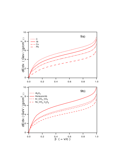
Figure 12: Energy loss of a magnetic monopole in various materials. These $\rmd E/\rmd x$ curves are for a magnetic charge value of $2|m^{\prime}|=n=1$; apart from the correction terms $K(|n|)$ and $B(|n|)$, we multiply by $n^{2}$ for larger magnetic charge values.

9 Binding

To this point in this review, we have concentrated on the scattering of monopoles with charged particles, or on dyon-dyon scattering. Now we turn to the question of the binding of these particles. Our discussion will be largely, although not exclusively, based on the nonrelativistic description.

If $q=e_{1}e_{2}+g_{1}g_{2}<0$, and $m^{\prime}=-(e_{1}g_{2}-e_{2}g_{1})/\hbar c$, ${\cal H}_{\rm NR}$ (2.2difgknopsacaeanbgbncdcecodgdv) gives binding:

$$E_{Nj}=-\frac{\mu}{2}q^{2}\left[N+\frac{1}{2}+\left((j+1/2)^{2}-m^{\prime 2}\right)^{1/2}\right]^{-2},$$ (2.2difgknopsacaeanbgbncdcecodgdxdzcfkvaaacakbbbhbqbvbycacdcedlefijba)

where $N$ is a principal quantum number. We will not further address the issue of dyons [135, 136, 137, 138, 139, 140], which for the correct sign of the electric charge will always bind electrically to nuclei. Monopoles will not bind this way; rather, a magnetic moment coupling as in (2.2difgknopsacaeanbgbncdcecodgdxdzeg) is required; for example, for spin-1/2,

$${\cal H}_{S}=-\frac{e\hbar}{2\mu c}\gamma\mbox{\boldmath{$\sigma$}}\cdot{\bf B},\qquad\gamma=1+\kappa=\frac{g}{2}.$$ (2.2difgknopsacaeanbgbncdcecodgdxdzcfkvaaacakbbbhbqbvbycacdcedlefijbb)

($\gamma=1$ or $g=2$ is the “normal” value.)

Suppose monopoles are produced in a collision at the Tevatron, for example; they travel through the detector, losing energy in a well-known manner (see, e.g., [27], which results are summarized in section 8), presumably ranging out, and eventually binding to matter in the detector (Be, Al, Pb, for example). The purpose of this section is to review the theory of the binding of magnetic charges to matter.

We consider the binding of a monopole of magnetic charge $g$ to a nucleus of charge $Ze$, mass ${\cal M}=Am_{p}$, and magnetic moment

$$\mbox{\boldmath{$\mu$}}={e\over m_{p}c}\gamma{\bf S},$$ (2.2difgknopsacaeanbgbncdcecodgdxdzcfkvaaacakbbbhbqbvbycacdcedlefijbc)

$\bf S$ being the spin of the nucleus. (We will assume here that the monopole mass $\gg{\cal M}$, which restriction could be easily removed.) The charge quantization condition is given by (2.2dia). Because the nuclear charge is $Ze$, the relevant angular momentum quantum number is ($m^{\prime}$ being an integer or an integer plus 1/2)

$$l=|m^{\prime}|Z.$$ (2.2difgknopsacaeanbgbncdcecodgdxdzcfkvaaacakbbbhbqbvbycacdcedlefijbd)

9.1 Nonrelativistic binding for $S=1/2$

In this subsection we follow the early work of Malkus [141] and the more recent papers of Bracci and Fiorentini [142, 143, 144, 145]. (There are also the results given in [146], but this reference seems to contain errors.)

The neutron ($Z=0$) is a special case. Binding will occur in the lowest angular momentum state, $J=1/2$, if

$$|\gamma|>{3\over 4|m^{\prime}|}$$ (2.2difgknopsacaeanbgbncdcecodgdxdzcfkvaaacakbbbhbqbvbycacdcedlefijbe)

Since $\gamma_{n}=-1.91$, this condition is satisfied for all $m^{\prime}$.

In general, it is convenient to define a reduced gyromagnetic ratio,

$$\hat{\gamma}={A\over Z}\gamma,\quad\hat{\kappa}=\hat{\gamma}-1.$$ (2.2difgknopsacaeanbgbncdcecodgdxdzcfkvaaacakbbbhbqbvbycacdcedlefijbf)

This expresses the magnetic moment in terms of the mass and charge of the nucleus. Binding will occur in the special lowest angular momentum state $J=l-{1\over 2}$ if

$$\hat{\gamma}>1+{1\over 4l}.$$ (2.2difgknopsacaeanbgbncdcecodgdxdzcfkvaaacakbbbhbqbvbycacdcedlefijbg)

Thus binding can occur here only if the anomalous magnetic moment $\hat{\kappa}>1/4l$. The proton, with $\kappa=1.79$, will bind.

Binding can occur in higher angular momentum states $J$ if and only if

$$|\hat{\kappa}|>\kappa_{c}={1\over l}\left|J^{2}+J-l^{2}\right|.$$ (2.2difgknopsacaeanbgbncdcecodgdxdzcfkvaaacakbbbhbqbvbycacdcedlefijbh)

For example, for $J=l+{1\over 2}$, $\kappa_{c}=2+3/4l$, and for $J=l+{3\over 2}$, $\kappa_{c}=4+15/4l$. Thus ${}^{3}_{2}$He, which is spin 1/2, will bind in the first excited angular momentum state because $\hat{\kappa}=-4.2$.

Unfortunately, to calculate the binding energy, one must regulate the potential at $r=0$. The results shown in table 1 assume a hard core.

9.2 Nonrelativistic binding for general $S$

The reference here is [147]. The assumption made here is that $l\geq S$. (There are only 3 exceptions, apparently: ²H, ⁸Li, and ¹⁰B.)

Binding in the lowest angular momentum state $J=l-S$ is given by the same criterion (2.2difgknopsacaeanbgbncdcecodgdxdzcfkvaaacakbbbhbqbvbycacdcedlefijbg) as in spin 1/2. Binding in the next state, with $J=l-S+1$, occurs if $\lambda_{\pm}>{1\over 4}$ where

$$\lambda_{\pm}=\left(S-{1\over 2}\right){\hat{\gamma}\over S}l-2l-1\pm\sqrt{(1+l)^{2}+(2S-1-l){\hat{\gamma}\over S}l+{1\over 4}l^{2}\left({\hat{\gamma}\over S}\right)^{2}}.$$ (2.2difgknopsacaeanbgbncdcecodgdxdzcfkvaaacakbbbhbqbvbycacdcedlefijbi)

The previous result for $S=1/2$ is recovered, of course. $S=1$ is a special case: Then $\lambda_{-}$ is always negative, while $\lambda_{+}>{1\over 4}$ if $\hat{\gamma}>\gamma_{c}$, where

$$\gamma_{c}={3\over 4l}{(3+16l+16l^{2})\over 9+4l}.$$ (2.2difgknopsacaeanbgbncdcecodgdxdzcfkvaaacakbbbhbqbvbycacdcedlefijbj)

For higher spins, both $\lambda_{\pm}$ can exceed $1/4$:

$$\lambda_{+}>{1\over 4} \hat{\gamma}>\gamma_{c-}$$ for (2.2difgknopsacaeanbgbncdcecodgdxdzcfkvaaacakbbbhbqbvbycacdcedlefijbka)

$$\lambda_{-}>{1\over 4} \hat{\gamma}>\gamma_{c+}$$ for (2.2difgknopsacaeanbgbncdcecodgdxdzcfkvaaacakbbbhbqbvbycacdcedlefijbkb)

where for $S={3\over 2}$

$$(\gamma_{c})_{\mp}={3\over 4l}(6+4l\mp\sqrt{33+32l}).$$ (2.2difgknopsacaeanbgbncdcecodgdxdzcfkvaaacakbbbhbqbvbycacdcedlefijbkl)

For ${}_{4}^{9}$Be, for which $\hat{\gamma}=-2.66$, we cannot have binding because $3>\gamma_{c-}>1.557$, $3<\gamma_{c+}<8.943$, where the ranges come from considering different values of $2|m^{\prime}|$ from 1 to $\infty$. For $S={5\over 2}$,

$$(\gamma_{c})_{\mp}={36+28l\mp\sqrt{1161+1296l+64l^{2}}\over 12l}.$$ (2.2difgknopsacaeanbgbncdcecodgdxdzcfkvaaacakbbbhbqbvbycacdcedlefijbkm)

So ${}^{27}_{13}$Al will bind in either of these states, or the lowest angular momentum state, because $\hat{\gamma}=7.56$, and $1.67>\gamma_{c-}>1.374$, $1.67<\gamma_{c+}<4.216$.

9.3 Relativistic spin-1/2

Kazama and Yang treated the Dirac equation [36]. See also [148, 149] and [135, 136, 137, 138, 139, 140].

In addition to the bound states found nonrelativistically, deeply bound states, with $E_{\rm binding}=\mathcal{M}$ are found. These states always exist for $J\geq l+1/2$. For $J=l-1/2$, these (relativistic) $E=0$ bound states exist only if $\kappa>0$. Thus (modulo the question of form factors) Kazama and Yang [36] expect that electrons can bind to monopoles. (We suspect that one must take the existence of these deeply bound states with a fair degree of skepticism. See also [150].)

As expected, for $J=l-1/2$ we have weakly bound states only for $\kappa>1/4l$, which is the same as the nonrelativistic condition (2.2difgknopsacaeanbgbncdcecodgdxdzcfkvaaacakbbbhbqbvbycacdcedlefijbg), and for $J\geq l+1/2$, only if $|\hat{\kappa}|>\kappa_{c}$, where $\kappa_{c}$ is given in (2.2difgknopsacaeanbgbncdcecodgdxdzcfkvaaacakbbbhbqbvbycacdcedlefijbh).

9.4 Relativistic spin-1

Olsen, Osland, and Wu considered this situation [151, 152].

In this case, no bound states exist, unless an additional interaction is introduced (this is similar to what happens nonrelativistically, because of the bad behavior of the Hamiltonian at the origin). Bound states are found if an “induced magnetization” interaction (quadratic in the magnetic field) is introduced. Binding is then found for the lowest angular momentum state $J=l-1$ again if $\hat{\kappa}>1/4l$. For the higher angular momentum states, the situation is more complicated:

• for $J=l$: bound states require $l\geq 16$, and

• for $J\geq l+1$: bound states require $J(J+1)-l^{2}\geq 25$.

But these results are probably highly dependent on the form of the additional interaction. The binding energies found are inversely proportional to the strength $\lambda$ of this extra interaction.

Table 1: Weakly bound states of nuclei to a magnetic monopole. The angular momentum quantum number $J$ of the lowest bound state is indicated. In Notes, NR means nonrelativistic and R relativistic calculations; hc indicates an additional hard core interaction is assumed, while FF signifies use of a form factor. IM represents induced magnetization, the additional interaction employed for the relativistic spin-1 calculation. We use $|m^{\prime}|=1/2$ except for the deuteron, where $|m^{\prime}|=1$ is required for binding.

Nucleus	Spin	$\gamma$	$\hat{\gamma}$	$J$	$E_{b}$	Notes	Ref
$n$	${1\over 2}$	$-1.91$		${1\over 2}$	350 keV	NR,hc	[146]
${}_{1}^{1}$H	${1\over 2}$	2.79	2.79	$l-{1\over 2}=0$	15.1 keV	NR,hc	[142]
					320 keV	NR,hc	[146]
					50–1000 keV	NR,FF	[147]
					263 keV	R	[148, 149]
${}_{1}^{2}$H	$1$	$0.857$	1.71	$l-1=0$ ($|m^{\prime}|=1$)	${130\over\lambda}$ keV	R,IM	[151, 152]
${}_{2}^{3}$He	${1\over 2}$	$-2.13$	$-3.20$	$l+{1\over 2}={3\over 2}$	13.4 keV	NR,hc	[142]
${}_{13}^{27}$Al	${5\over 2}$	3.63	7.56	$l-{5\over 2}=4$	2.6 MeV	NR,FF	[148, 149]
${}_{13}^{27}$Al	${5\over 2}$	3.63	7.56	$l-{5\over 2}=4$	560 keV	NR,hc	[153]
${}_{48}^{113}$Cd	${1\over 2}$	$-0.62$	$-1.46$	$l+{1\over 2}={49\over 2}$	6.3 keV	NR,hc	[142]

9.5 Remarks on binding

Clearly, this summary indicates that the theory of monopole binding to nuclear magnetic dipole moments is rather primitive. The angular momentum criteria for binding is straightforward; but in general (except for relativistic spin 1/2) additional interactions have to be inserted by hand to regulate the potential at $r=0$. The results for binding energies clearly are very sensitive to the nature of that additional interaction. It cannot even be certain that binding occurs in the allowed states. In fact, however, it seems nearly certain that monopoles will bind to all nuclei, even, for example, Be, because the magnetic field in the vicinity of the monopole is so strong that the monopole will disrupt the nucleus and will bind to the nuclear, or even the subnuclear, constituents.

9.6 Binding of monopole-nucleus complex to material lattice

Now the question arises: Can the magnetic field in the detector extract the monopole from the nucleus that binds it? And if not, is the bound complex of nucleus and monopole rigidly attached to the crystalline lattice of the material? To answer the former question we regard it as a simple tunneling situation. The decay rate is estimated by the WKB formula

$$\Gamma\sim{1\over a}\exp\left[-\frac{2}{\hbar}\int_{a}^{b}\rmd r\sqrt{2{\cal M}(V-E)}\right],$$ (2.2difgknopsacaeanbgbncdcecodgdxdzcfkvaaacakbbbhbqbvbycacdcedlefijbkna)

where the potential is crudely that due to the dipole interaction and the external magnetic field,

$$V=-{\mu g\over r^{2}}-gBr,$$ (2.2difgknopsacaeanbgbncdcecodgdxdzcfkvaaacakbbbhbqbvbycacdcedlefijbknb)

$\cal M$ is the nuclear mass $\ll$ monopole mass, and the inner and outer turning points, $a$ and $b$ are the zeroes of $E-V$. Provided the following equality holds,

$$(-E)^{3}\gg g^{3}\mu B^{2},$$ (2.2difgknopsacaeanbgbncdcecodgdxdzcfkvaaacakbbbhbqbvbycacdcedlefijbkno)

which should be very well satisfied, since the right hand side is about $10^{-19}|m^{\prime}|^{3}$ MeV³, for the CDF field of $B=1.5$ T, we can write the decay rate as

$$\Gamma\sim|m^{\prime}|^{-1/2}10^{23}\mbox{s}^{-1}\exp\left[-{4\sqrt{2}\over 3\cdot 137}\left({-E\over m_{e}}\right)^{3/2}{B_{0}\over|m^{\prime}|B}A^{1/2}\left({m_{p}\over m_{e}}\right)^{1/2}\right],$$ (2.2difgknopsacaeanbgbncdcecodgdxdzcfkvaaacakbbbhbqbvbycacdcedlefijbknp)

where the characteristic field, defined by $eB_{0}=m^{2}_{e}$, is $4\times 10^{9}$ T. If we put in $B=1.5$ T, and $A=27$, $-E=2.6$MeV, appropriate for ${}_{13}^{27}$Al, we have for the exponent, for $m^{\prime}=1/2$, $-2\times 10^{11}$, corresponding to a rather long time! To get a 10 yr lifetime, the binding energy would have to be only of the order of 1 eV. Monopoles bound with kilovolt or more energies will stay around forever.

Then the issue is whether the entire Al atom-monopole complex can be extracted with the 1.5 T magnetic field present in CDF. The answer seems to be unequivocally no. The point is that the atoms are rigidly bound in a lattice, with no nearby site into which they can jump. A major disruption of the lattice would be required to dislodge the atoms, which would probably require kilovolts of energy. Some such disruption was made by the monopole when it came to rest and was bound in the material, but that disruption would be very unlikely to be in the direction of the accelerating magnetic field. Again, a simple Boltzmann argument shows that any effective binding slightly bigger than 1 eV will result in monopole trapping “forever.” This argument applies equally well to binding of monopoles in ferromagnets. If monopoles bind strongly to nuclei there, they will not be extracted by 5 T fields, contrary to the arguments of Goto et al[154]. The corresponding limits on monopoles from ferromagnetic samples of Carrigan et al[155] are suspect.

10 Searches for magnetic monopoles

With the advent of “more unified” non-Abelian theories, classical composite monopole solutions were discovered, as briefly discussed in section 4. The mass of these monopoles would be of the order of the relevant gauge-symmetry breaking scale, which for grand unified theories is of order $10^{16}$ GeV or higher. But there are models where the electroweak symmetry breaking can give rise to monopoles of mass $\sim 10$ TeV [63, 64, 65, 66]. Even the latter are not yet accessible to accelerator experiments, so limits on heavy monopoles depend either on cosmological considerations (see for example [156]) or detection of cosmologically produced (relic) monopoles impinging upon the earth or moon [24, 25, 157, 158, 159, 160, 161, 162]. Since the revival of interest in monopoles in the 1970s, there have been two well-known announcements of their discovery: that of Price et al[163], who found an cosmic ray track etched in a plastic detector, and that of Cabrera [158], who reported a single event in a induction loop. The former interpretation was immediately refuted by Alvarez [164], while the latter has never been duplicated, so is presumed spurious.

However, a priori, there is no reason that Dirac/Schwinger monopoles or dyons of arbitrary mass might not exist: In this respect, it is important to set limits below the 1 TeV scale.

10.1 Direct searches

In this review we will concentrate on recently obtained limits, since periodic reviews of the status of magnetic monopole searches have been published [165, 166]. Before 2000, the best previous direct limit on magnetic monopoles was that obtained at Fermilab by Bertani et al[167] who obtained cross section limits of $2\times 10^{-34}$ cm² for monopole masses below 850 GeV. As we shall see below, the Oklahoma experiment [21], while not extending to as high masses, gives cross section limits some two orders of magnitude smaller. The recent CDF experiment [168] sets a three order of magnitude improvement over [167]. (In contrast to [165, 166], we call all of these experiments “direct,” whether they are searching for previously produced monopoles trapped in material or the ionization and radiation produced by monopoles passing through a detector.) As noted in section 9.6 there have been experiments to search for monopoles by extracting them from matter with strong magnetic fields [155, 169]; as remarked there, it is doubtful such an experiment would succeed, since the binding energy of a monopole to the lattice is probably at least in the keV range, while the energy acquired by a Dirac monopole in a 100 kG field over an atomic distance is only 20 eV.

Cosmologically produced monopoles are commonly assumed to arise from a GUT (Grand Unified Theory) where a grand unified group such as SU(5) breaks down into the standard model group SU(3)$\times$SU(2)$\times$U(1). Barring premature unification due to, say, large extra dimensions, the mass of such a monopole is expected to be of the order $10^{16}$ GeV, so they are incapable of being produced in accelerators. However, since in the early universe at least one monopole should be produced per causal domain, too many monopoles would have been produced [170, 171], and would come into conflict with the Parker bound, which states that cosmic fields would be quenched if the density of magnetic monopoles is too high [172]. This is one of the problems solved by inflation.

Various experiments have been conducted to look for cosmic monopoles. An interesting limit comes from the Rubakov-Callan mechanism for monopole catalysis of proton decay [173, 174],

$$M+p\to M+e^{+}+\pi^{0},$$ (2.2difgknopsacaeanbgbncdcecodgdxdzcfkvaaacakbbbhbqbvbycacdcedlefijbkna)

where MACRO [175] found a limit on the flux of 3–8$\times 10^{-16}$ cm^-2 s^-1 sr^-1. However, MACRO’s best limit [176], based on scintillation counters, limited streamer tubes, and nuclear track detectors, give a much better limit of $1.4\times 10^{-16}$ cm^-2 s^-1 sr^-1 for monopole velocities in the range $4\times 10^{-5}<\beta<1$, roughly a factor of two improvement over previous limits, and well below the Parker bound of $\sim 10^{-15}$ cm^-2 s^-1 sr^-1. Even smaller limits depend on the mechanism by which a monopole would produce a track in ancient mica [177, 178]. One should note that lower mass monopoles, with masses of order $10^{10}$ GeV, arising from intermediate stages of symmetry breaking below the GUT scale, would not catalyze proton decay [179, 180], but the more stringent MACRO limits still apply.

We will discuss the three recent direct search limits in sections 11–13.

10.2 Indirect searches

In the above, and in the following sections, we discussed direct searches, where the monopoles are searched for as free particles. The indirect searches that have been proposed and carried out rely on effects attributable to the virtual existence of monopoles. De Rújula in 1995 [181] proposed looking at the three-photon decay of the $Z$ boson, where the process proceeds through a virtual monopole loop, as shown in figure 13. If we use his formula for the branching ratio for the $Z\to 3\gamma$ process, compared to the current experimental upper limit [182] for the branching ratio of $10^{-5}$, we can rule out monopole masses lower than about 400 GeV, rather than the 600 GeV quoted by De Rújula. Similarly, Ginzburg and Panfil in 1982 [183] and more recently Ginzburg and Schiller in 1999 [184, 185] considered the production of two photons with high transverse momenta by the collision of two photons produced either from $e^{+}e^{-}$ or $q\overline{q}$ collisions. Again the final photons are produced through a virtual monopole loop. Based on this theoretical scheme, an experimental limit was given by the D0 collaboration [186], which sets the following bounds on the monopole mass $M$:

$$\frac{M}{2|m^{\prime}|}>\left\{\begin{array}[]{cc}610\mbox{ GeV}&\mbox{ for }S=0\\ 870\mbox{ GeV}&\mbox{ for }S=1/2\\ 1580\mbox{ GeV}&\mbox{ for }S=1\end{array}\right.,$$ (2.2difgknopsacaeanbgbncdcecodgdxdzcfkvaaacakbbbhbqbvbycacdcedlefijbknb)

where $S$ is the spin of the monopole, and $m^{\prime}=eg$ is the magnetic charge quantization number.

It is worth noting that a lower mass limit of 120 GeV for a Dirac monopole has been set by Graf, Schäfer, and Greiner [187], based on the monopole contribution to the vacuum polarization correction to the muon anomalous magnetic moment. (Actually, we believe that the correct limit, obtained from the well-known textbook formula for the $g$-factor correction due to a massive Dirac particle is 60 GeV.)

10.2.1 Difficulty with indirect limits

The indirect limits mentioned above rely up the Feynman graph shown in figure 13.

Figure 13: The light-by-light scattering graph for either an electron or a monopole loop.

If the particle in the loop is an ordinary electrically charged electron, this process is well-known. If, further, the photons involved are of very low momentum compared the the mass of the electron, then the result may be simply derived from the well-known Euler-Heisenberg Lagrangian [188, 189, 190] which for a spin-1/2 charged-particle loop in the presence of weak homogeneous electric and magnetic fields is

$${\cal L} = -\frac{1}{16\pi}F^{2}+\frac{\alpha^{2}}{360}\frac{1}{m^{4}}\frac{1}{(4\pi)^{2}}[4(F^{2})^{2}+7(F{}^{*}F)^{2}],$$ (2.2difgknopsacaeanbgbncdcecodgdxdzcfkvaaacakbbbhbqbvbycacdcedlefijbknc)

where $m$ is the mass of the particle in the loop. The Lagrangian for a spin-0 and spin-1 charged particle in the loop is given by similar formulas, which are derived in [190, 191] and (implicitly) in Ref. [192, 193, 194], respectively.

Given this homogeneous-field effective Lagrangian, it is a simple matter to derive the cross section for the $\gamma\gamma\to\gamma\gamma$ process in the low energy limit. (These results can, of course, be directly calculated from the corresponding one-loop Feynman graph with on-mass-shell photons. See [191, 195].) Explicit results for the differential cross section are given in textbooks:

$$\frac{\rmd\sigma}{\rmd\Omega}=\frac{139}{32400\pi^{2}}\alpha^{4}\frac{\omega^{6}}{m^{8}}(3+\cos^{2}\theta)^{2},$$ (2.2difgknopsacaeanbgbncdcecodgdxdzcfkvaaacakbbbhbqbvbycacdcedlefijbknd)

and the total cross section for a spin-1/2 charged particle in the loop is

$$\sigma=\frac{973}{10125\pi}\alpha^{4}\frac{\omega^{6}}{m^{8}},\qquad\omega/m\ll 1,\qquad s=4\omega^{2}.$$ (2.2difgknopsacaeanbgbncdcecodgdxdzcfkvaaacakbbbhbqbvbycacdcedlefijbkne)

The numerical coefficient in the total cross section are $0.00187$, $0.0306$, and $3.50$ for spin 0, spin 1/2, and spin 1 particles in the loop, respectively.

How is this applicable to photon scattering through a monopole loop? This would seem impossible because of the existence of the string, which renders perturbation theory meaningless. Of course, no one has attempted a calculation of the “box” diagram with the monopole interaction. Rather, De Rújula and Ginzburg (explicitly or implicitly) appeal to duality, that is, the dual symmetry (2.2a) that the introduction of magnetic charge brings to Maxwell’s equations:

$${\bf E}\to{\bf B},\qquad{\bf B}\to-{\bf E},$$ (2.2difgknopsacaeanbgbncdcecodgdxdzcfkvaaacakbbbhbqbvbycacdcedlefijbknf)

and similarly for charges and currents. Thus the argument is that for low energy photon processes it suffices to compute the fermion loop graph in the presence of zero-energy photons, that is, in the presence of static, constant fields. Since the Euler-Heisenberg Lagrangian is invariant under the duality substitution on the fields alone, this means we obtain the low energy cross section $\sigma_{\gamma\gamma\to\gamma\gamma}$ through the monopole loop from the equation for the QED cross section by the substitution $e\to g$, or

$$\alpha\to\alpha_{g}=137m^{\prime 2},\qquad 2|m^{\prime}|=1,2,3,\dots.$$ (2.2difgknopsacaeanbgbncdcecodgdxdzcfkvaaacakbbbhbqbvbycacdcedlefijbkng)

It is critical to emphasize that the Euler-Heisenberg Lagrangian is an effective Lagrangian for calculations at the one fermion loop level for low energy, i.e., $\omega/m\ll 1$. However, it becomes unreliable if radiative corrections are large. (The same has been noted in another context by Bordag, Robaschik, Wieczorek, and Lindig [196, 197].) For example, the internal radiative correction to the box diagram have been computed by Ritus [198] and by Reuter, Schmidt, and Schubert [199, 200] in QED. In the $O(\alpha^{2})$ term in the expansion of the EH Lagrangian (2.2difgknopsacaeanbgbncdcecodgdxdzcfkvaaacakbbbhbqbvbycacdcedlefijbknc), the coefficients of the $(F^{2})^{2}$ and the $(F\tilde{F})^{2}$ terms are multiplied by

$$\left(1+\frac{40}{9}\frac{\alpha}{\pi}+O(\alpha^{2})\right)\quad\mbox{and}\quad\left(1+\frac{1315}{252}\frac{\alpha}{\pi}+O(\alpha^{2})\right),$$ (2.2difgknopsacaeanbgbncdcecodgdxdzcfkvaaacakbbbhbqbvbycacdcedlefijbknh)

respectively. The corrections become meaningless when we replace $\alpha\to\alpha_{g}$.

10.2.2 Unitarity bound

This would seem to be a devastating objection to the results given by Ginzburg et al[184, 185] and used in the D0 analysis [186]. But even if one closes one’s eyes to higher order effects, it seems clear that the mass limits quoted are inconsistent.

If we take the cross section given by (2.2difgknopsacaeanbgbncdcecodgdxdzcfkvaaacakbbbhbqbvbycacdcedlefijbkne) and make the duality substitution, we obtain for the low energy light-by-light scattering cross section in the presence of a monopole loop ($M$ is the monopole mass)

$$\sigma_{\gamma\gamma\to\gamma\gamma}\approx\frac{973}{10125\pi}\frac{m^{\prime 8}}{\alpha^{4}}\frac{\omega^{6}}{M^{8}}=1.08\times 10^{7}\,m^{\prime 8}\frac{1}{M^{2}}\left(\frac{\omega}{M}\right)^{6}.$$ (2.2difgknopsacaeanbgbncdcecodgdxdzcfkvaaacakbbbhbqbvbycacdcedlefijbkni)

If the cross section were dominated by a single partial wave of angular momentum $J$, the cross section would be bounded by

$$\sigma\leq\frac{\pi(2J+1)}{s}\sim\frac{3\pi}{s},\qquad J\sim 1.$$ (2.2difgknopsacaeanbgbncdcecodgdxdzcfkvaaacakbbbhbqbvbycacdcedlefijbknj)

Comparing this with the cross section given above, we obtain the following inequality for the cross section to be consistent with unitarity,

$$\frac{M}{\omega}\geq 6|m^{\prime}|.$$ (2.2difgknopsacaeanbgbncdcecodgdxdzcfkvaaacakbbbhbqbvbycacdcedlefijbknk)

But the limits quoted by D0 for the monopole mass are less than this:

$$\frac{M}{2|m^{\prime}|}>870\mbox{ GeV},\quad\mbox{spin }1/2,$$ (2.2difgknopsacaeanbgbncdcecodgdxdzcfkvaaacakbbbhbqbvbycacdcedlefijbknl)

because, at best, a minimum estimate is $\langle\omega\rangle\sim 300$ GeV, so the theory cannot sensibly be applied below a monopole mass of about 1 TeV. (Note that changing the value of $J$ in the unitarity limits has very little effect on the bound since an 8th root is taken: Replacing $J$ by 50 reduces the limit only by 50%.)

Similar remarks can be directed toward the De Rújula limits [181]. That author, however, notes the “perilous use of a perturbative expansion in $g$.” However, although he writes down the correct vertex, he does not, in fact, use it, instead appealing to duality, and even so he admittedly omits enormous radiative corrections of $O(\alpha_{g})$ without any justification other than what we believe is a specious reference to the use of effective Lagrangian techniques for these processes.

As we will see, some of the same objections apply to the direct search limits. The advantage, however, of the latter, is that the signal of a positive event is more unambiguous, and in the Oklahoma and H1 experiments, a monopole, if found, would be available for further study.

11 Oklahoma experiment: Fermilab E882

The best prior experimental limit on the direct accelerator production of magnetic monopoles is that of Bertani et alin 1990 [167] (see also Price et al[201, 202]):

$$\sigma\leq 2\times 10^{-34}\mbox{cm}^{2}\quad\mbox{for a monopole mass}\quad M\leq 850\,\mbox{GeV}.$$ (2.2difgknopsacaeanbgbncdcecodgdxdzcfkvaaacakbbbhbqbvbycacdcedlefijbkna)

The fundamental mechanism is supposed to be a Drell-Yan process,

$$p+\bar{p}\to M+\bar{M}+X,$$ (2.2difgknopsacaeanbgbncdcecodgdxdzcfkvaaacakbbbhbqbvbycacdcedlefijbknb)

where the cross section is given by

$$\frac{\rmd\sigma}{\rmd\mathcal{M}}=(68.5n^{2})^{2}\beta^{3}\frac{8\pi\alpha^{2}}{9s}\int\frac{\rmd x_{1}}{x_{1}}\sum_{i}Q_{i}^{2}q_{i}(x_{1})\bar{q}_{i}\left(\frac{\mathcal{M}^{2}}{sx_{1}}\right).$$ (2.2difgknopsacaeanbgbncdcecodgdxdzcfkvaaacakbbbhbqbvbycacdcedlefijbknc)

Here $\mathcal{M}$ is the invariant mass of the monopole-antimonopole pair, and we have included a factor of $\beta^{3}$ to reflect (1) phase space and (2) the velocity suppression of the magnetic coupling, as roughly implied by (2.2difgknopsacaeanbgbncdcecodgdxdzcfg)–See also (2.2dip). Note that we are unable to calculate the elementary process

$$q\bar{q}\to\gamma^{*}\to M\bar{M}$$

perturbatively, so we must use nonperturbative estimates.

Any monopole produced at Fermilab is trapped in the detector elements with 100% probability due to interaction with the magnetic moments of the nuclei, based on the theory described in section 9. The experiment consists of running samples obtained from the old D0 and CDF detectors through a superconducting induction detector. Figure 14 is a sketch of the D0 detector.

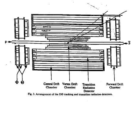
Figure 14: Arrangement of the D0 tracking and transition radiation detectors.

We are able to set much better limits than Bertani et al[167] because the integrated luminosity is $10^{4}$ times that of the previous 1990 experiment:

$$\int{\cal L}=172\pm 8\,\mbox{pb}^{-1}\quad(\mbox{D0}).$$ (2.2difgknopsacaeanbgbncdcecodgdxdzcfkvaaacakbbbhbqbvbycacdcedlefijbknd)

We use energy loss formula of Ahlen [133, 132, 203], as described in section 8. The graph in figure 12 shows the energy loss $\rmd E/\rmd x$ for various materials.

Figure 15 is a diagram of the OU magnetic monopole induction detector. It is a cylindrical detector, with a warm bore of diameter 10 cm, surrounded by a cylindrical liquid N₂ dewer, which insulated a liquid He dewer. The superconducting loop detectors were within the latter, concentric with the warm bore. Any current established in the loops was detected by a SQUID. The entire system was mechanically isolated from the building, and magnetically isolated by $\mu$ metal and superconducting lead shields. The magnetic field within the bore was reduced with the help of Helmholtz coils to about 1% of the earth’s field. Samples were pulled vertically through the warm bore with a computer controlled stepper motor. Each traversal took about 50 s; every sample run consisted of some 20 up and down traversals. Most samples were run more than once, and more than 660 samples of Be, Pb, and Al from both the old CDF and D0 detectors were analyzed over a period of 7 years.

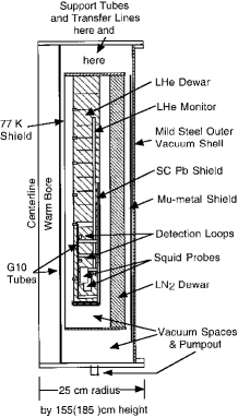
Figure 15: Sketch of the OU induction detector. Shown is a vertical cross section; it should be imagined as rotated about the vertical axis labelled “centerline.”

11.1 Monopole induced signal

Note that if the shield were not present, the supercurrent induced by a monopole of strength $g$ passing through a loop of radius $r$ and inductance $L$ would be given by

$$I(t)=\frac{2\pi g}{Lc}\left(1-\frac{z(t)}{\sqrt{r^{2}+z(t)^{2}}}\right),$$ (2.2difgknopsacaeanbgbncdcecodgdxdzcfkvaaacakbbbhbqbvbycacdcedlefijbkne)

where $z(t)$ is the vertical position of the monopole relative to the position of the center of the loop. A more detailed theory is described in the following. The theory can be verified with a pseudopole, which is a long, $\sim 1$ m, electromagnetic solenoid, which produces a field near one end very similar to that produced by a pure magnetic pole. The excellent agreement between theory and experiment is indicated in figure 16.

Figure 16: Typical step plots: D0 aluminum, CDF lead, and CDF aluminum. The experimental data was collected from pseudopole simulations; the steps shown are for the difference between the results with reversed polarizations of the pseudopole. Data agrees well with the theory which incorporates the effect of the shielded superconducting loops. The theory without the shield, given by Barger and Ollson [204], is also shown.

11.1.1 Simplified theory of monopole detector

This subsection describes the basis of the functioning of our magnetic monopole detector. It works by detecting the magnetic flux intercepted by a superconducting loop contained within a superconducting cylinder. The detector is sketched in figure 17.

Figure 17: Diagram of monopole detector. The monopole $g$ is assumed to be on the central axis at a height $z^{\prime}$ above the bottom of the detector, which we model as a cylindrical perfectly conducting can of radius $a$, closed at the bottom. The superconducting loop of radius $r$ is a height $Z$ above the base.

In order to incorporate finite-size effects, we consider first a perfectly conducting right circular cylinder of radius $a$ of semi-infinite length, with axis along the $z$-axis, and with a perfectly conducting circular bottom cap at $z=0$. We use cylindrical coordinates $\rho$, $\theta$, and $z$.

Because the boundaries are superconductors, the normal component of $\bf B$ must vanish on the surfaces, that is,

$$B_{\rho}\bigg{|}_{{\rho=a}\atop{z>0}}=0,\quad B_{z}\bigg{|}_{z=0}=0.$$ (2.2difgknopsacaeanbgbncdcecodgdxdzcfkvaaacakbbbhbqbvbycacdcedlefijbknf)

Now suppose a magnetic pole of strength $g$ is placed on the $z$ axis at $z=z^{\prime}>0$. This could either be a magnetic monopole (magnetic charge) or one pole of a very long electromagnet (“pseudopole”). Imagine a circular conducting loop of radius $r<a$ centered on the axis of the cylinder and perpendicular to that axis, with center at $z=Z$. Inside the cylinder and outside of the loop, $\bf B$ is derivable from a magnetic scalar potential,

$${\bf B}=-\mbox{\boldmath{$\nabla$}}\phi_{M},$$ (2.2difgknopsacaeanbgbncdcecodgdxdzcfkvaaacakbbbhbqbvbycacdcedlefijbkng)

since we may ignore the displacement current, because the time variation is negligible. $\phi_{M}$ satisfies Poisson’s equation, in cylindrical coordinates:

$$\mbox{\boldmath{$\nabla$}}\cdot\mathbf{B}=-\left(\frac{1}{\rho}\frac{\partial}{\partial\rho}\rho\frac{\partial}{\partial\rho}+\frac{1}{\rho^{2}}\frac{\partial^{2}}{\partial\theta^{2}}+\frac{\partial^{2}}{\partial z^{2}}\right)\phi_{M}=4\pi g\delta({\bf r-r^{\prime}}),$$ (2.2difgknopsacaeanbgbncdcecodgdxdzcfkvaaacakbbbhbqbvbycacdcedlefijbknh)

where $\mathbf{r}^{\prime}$ is the position of the monopole, $\mathbf{r^{\prime}}=(\rho^{\prime},\theta^{\prime},z^{\prime})$. This is the equation for a Green’s function, which we can express in separated variables form. That is, we write

$$\phi_{M}=\frac{2}{\pi}\int_{0}^{\infty}\rmd k\cos kz\cos kz^{\prime}\sum_{m=-\infty}^{\infty}\frac{1}{2\pi}\rme^{\rmi m(\theta-\theta^{\prime})}g_{m}(\rho,\rho^{\prime};k),$$ (2.2difgknopsacaeanbgbncdcecodgdxdzcfkvaaacakbbbhbqbvbycacdcedlefijbkni)

where, in view of the first boundary condition in (2.2difgknopsacaeanbgbncdcecodgdxdzcfkvaaacakbbbhbqbvbycacdcedlefijbknf), we may express the reduced Green’s function in terms of modified Bessel functions:

$$g_{m}(\rho,\rho^{\prime};k)=-4\pi gI_{m}(k\rho_{<})\left[K_{m}(k\rho_{>})-I_{m}(k\rho_{>})\frac{K^{\prime}_{m}(ka)}{I^{\prime}_{m}(ka)}\right],$$ (2.2difgknopsacaeanbgbncdcecodgdxdzcfkvaaacakbbbhbqbvbycacdcedlefijbknj)

where $\rho_{<}$ ($\rho_{>}$) is the lesser (greater) of $\rho$, $\rho^{\prime}$. If the monopole is confined to the $z$ axis, only the $m=0$ term survives:

$$\phi_{M}=-\frac{4g}{\pi}\int_{0}^{\infty}\rmd k\cos kz\cos kz^{\prime}\left[K_{0}(k\rho)+I_{0}(k\rho)\frac{K_{1}(ka)}{I_{1}(ka)}\right],$$ (2.2difgknopsacaeanbgbncdcecodgdxdzcfkvaaacakbbbhbqbvbycacdcedlefijbknk)

which uses

$$I_{0}^{\prime}(x)=I_{1}(x),\qquad K_{0}^{\prime}(x)=-K_{1}(x).$$ (2.2difgknopsacaeanbgbncdcecodgdxdzcfkvaaacakbbbhbqbvbycacdcedlefijbknl)

By integrating over the cross section of the loop using

$$\int_{0}^{x}\rmd t\,t\,K_{0}(t)=-x\,K_{1}(x)+1,\qquad\int_{0}^{x}\rmd t\,t\,I_{0}(t)=x\,I_{1}(x),$$ (2.2difgknopsacaeanbgbncdcecodgdxdzcfkvaaacakbbbhbqbvbycacdcedlefijbknm)

we obtain the following formula for the magnetic flux subtended by the loop,

$$\Phi=\int\rmd{\bf S\cdot B}=4\pi g\left[\eta(Z-z^{\prime})-F(Z,z^{\prime})\right],$$ (2.2difgknopsacaeanbgbncdcecodgdxdzcfkvaaacakbbbhbqbvbycacdcedlefijbknn)

where the step function is (2.2difgknopsacaea), and the response function is

$$F(z,z^{\prime})=\frac{2}{\pi}\frac{r}{a}\int_{0}^{\infty}\rmd x\,\sin x\frac{z}{a}\cos x\frac{z^{\prime}}{a}\left\{K_{1}(xr/a)-I_{1}(xr/a)\frac{K_{1}(x)}{I_{1}(x)}\right\}.$$ (2.2difgknopsacaeanbgbncdcecodgdxdzcfkvaaacakbbbhbqbvbycacdcedlefijbkno)

Now suppose that the pole is slowly moved from a point far above the loop, $z^{\prime}=+\infty$, to a point below the loop, $z^{\prime}=z_{0}$, $Z>z_{0}$. Then from Maxwell’s equation

$$\mbox{\boldmath{$\nabla$}}\times{\bf E}=-\frac{1}{c}\frac{\partial}{\partial t}{\bf B}-\frac{4\pi}{c}{\bf J}_{m},$$ (2.2difgknopsacaeanbgbncdcecodgdxdzcfkvaaacakbbbhbqbvbycacdcedlefijbknp)

where $\mathbf{J}_{m}$ is the magnetic current density, the emf induced in the loop is

$${\cal E}=\oint{\bf E}\cdot\rmd{\bf l},=-\frac{\rmd\Phi}{c\rmd t}+\frac{4\pi}{c}g\delta(t),$$ (2.2difgknopsacaeanbgbncdcecodgdxdzcfkvaaacakbbbhbqbvbycacdcedlefijbknq)

if $t=0$ is the time at which the pole passes through the plane of the loop. The net change in emf gives rise to a persistent current $I$ in the superconducting loop,

$$LI=\int_{-\infty}^{\infty}{\cal E}\rmd t=-\frac{1}{c}\Delta\Phi+\frac{4\pi}{c}g=\frac{4\pi}{c}gF(Z,z_{0}),$$ (2.2difgknopsacaeanbgbncdcecodgdxdzcfkvaaacakbbbhbqbvbycacdcedlefijbknr)

where $L$ is the inductance of the loop, and the response function $F$ is given in (2.2difgknopsacaeanbgbncdcecodgdxdzcfkvaaacakbbbhbqbvbycacdcedlefijbkno). This is just a statement of the Meissner effect, that the flux change caused by the moving monopole is cancelled by that due to the current set up in the loop.

When the loop is very far from the bottom cap, $Z\gg a$, only small $x$ contributes to the integral in Eq. (2.2difgknopsacaeanbgbncdcecodgdxdzcfkvaaacakbbbhbqbvbycacdcedlefijbkno), and it is easy to see that

$$\int_{-\infty}^{\infty}{\cal E}\rmd t=\frac{4\pi g}{c}\left(1-\frac{r^{2}}{a^{2}}\right),$$ (2.2difgknopsacaeanbgbncdcecodgdxdzcfkvaaacakbbbhbqbvbycacdcedlefijbkns)

so the signal is maximized by making the loop as small as possible, relative to the radius of the cylinder. We get the full flux of the monopole only for a loop in empty space, $a/r\to\infty$. This perhaps counterintuitive effect is due to the fact that the superconducting walls confine the magnetic flux to the interior of the cylinder. Thus for the superconducting can, the induced current in the detection loop caused by the passage of a monopole from $z^{\prime}=\infty$ to $z^{\prime}=0$ is

$$LI=\frac{4\pi g}{c}-\frac{\Delta\Phi}{c}=\frac{4\pi g}{c}-\frac{\Phi(z^{\prime}=0)}{c},$$ (2.2difgknopsacaeanbgbncdcecodgdxdzcfkvaaacakbbbhbqbvbycacdcedlefijbknt)

which yields the result (2.2difgknopsacaeanbgbncdcecodgdxdzcfkvaaacakbbbhbqbvbycacdcedlefijbkns) if one assumes that the magnetic field is uniform across the can’s cross section at the position of the loop when the pole is at the bottom, because all the flux must pass up through the can. If we consider, instead, an infinite, open-ended, superconducting cylinder, with the monopole passing from $z=+\infty$ to $z=-\infty$, at either extreme half the flux must cross the plane of the loop, so with the uniformity assumption we get the same result:

$$LI=\frac{4\pi g}{c}-\frac{\Delta\Phi}{c}=\frac{4\pi g}{c}\left(1-\frac{r^{2}}{a^{2}}\right).$$ (2.2difgknopsacaeanbgbncdcecodgdxdzcfkvaaacakbbbhbqbvbycacdcedlefijbknu)

The simple assumption of a uniform magnetic field is apparently justified by the exact result (2.2difgknopsacaeanbgbncdcecodgdxdzcfkvaaacakbbbhbqbvbycacdcedlefijbkns).

We conclude this discussion by noting how the exact calculation is modified for an infinite superconducting cylinder. In the magnetic scalar potential, the integral over $k$ mode functions in (2.2difgknopsacaeanbgbncdcecodgdxdzcfkvaaacakbbbhbqbvbycacdcedlefijbkni) is replaced by

$$\int_{-\infty}^{\infty}\frac{\rmd k}{2\pi}\rme^{\rmi k(z-z^{\prime})},$$ (2.2difgknopsacaeanbgbncdcecodgdxdzcfkvaaacakbbbhbqbvbycacdcedlefijbknv)

which has the effect of replacing the flux expression (2.2difgknopsacaeanbgbncdcecodgdxdzcfkvaaacakbbbhbqbvbycacdcedlefijbknn) by

$$\Phi=2\pi g[\epsilon(z-z^{\prime})-F(Z-z^{\prime},0)],$$ (2.2difgknopsacaeanbgbncdcecodgdxdzcfkvaaacakbbbhbqbvbycacdcedlefijbknw)

where $\epsilon(\xi)$ is given by (2.2difgknopsacaeb). Then the induced current in the detection loop when the monopole passes from a point above the loop $z^{\prime}=Z+\xi$ to a point, equidistant, below the loop, $z^{\prime}=Z-\xi$, is

$$LI=\frac{4\pi g}{c}F(\xi,0)\to\frac{4\pi g}{c}\left(1-\frac{r^{2}}{a^{2}}\right),$$ (2.2difgknopsacaeanbgbncdcecodgdxdzcfkvaaacakbbbhbqbvbycacdcedlefijbknx)

where the last limit applies if $\xi/a\gg 1$. This result coincides with that in (2.2difgknopsacaeanbgbncdcecodgdxdzcfkvaaacakbbbhbqbvbycacdcedlefijbkns). The function $R(\xi)=\frac{1}{2}F(\xi,0)/(1-r^{2}/a^{2})+\frac{1}{2}$, corresponding to a monopole starting from a point $z_{1}$ far above the loop, $z_{1}-Z\gg a$, and ending at a point $z_{0}=Z-\xi$, is plotted as a function of $\xi$ for our parameter values in figure 16c, where it is shown to agree well with experimental data. This response function coincides with the result obtained from (2.2difgknopsacaeanbgbncdcecodgdxdzcfkvaaacakbbbhbqbvbycacdcedlefijbknr), because

$$F(Z,Z-\xi)=\frac{1}{2}F(2Z-\xi,0)+\frac{1}{2}F(\xi,0)\approx\frac{1}{2}\left(1-\frac{r^{2}}{a^{2}}\right)+\frac{1}{2}F(\xi,0),$$ (2.2difgknopsacaeanbgbncdcecodgdxdzcfkvaaacakbbbhbqbvbycacdcedlefijbkny)

if $Z/a\gg 1$. This shows that the effect of the endcap (which of course is not present in actual detector) is negligible, demonstrating that the fact that the superconducting shield is of finite length is of no significance.

11.2 Background effects

All nonmagnetic but conducting samples possess:

• Permanent magnetic dipole moments $\mu$, which give rise to signals in free space of the form

  $$I(t)=-\frac{2\pi\mu_{z}}{Lc}\frac{r^{2}}{[r^{2}+z(t)^{2}]^{3/2}}$$ (2.2difgknopsacaeanbgbncdcecodgdxdzcfkvaaacakbbbhbqbvbycacdcedlefijbknz)

• Induced magnetization: Conducting samples passing though magnetic gradients with speed $v$ produce time-varying magnetic fields which induce signals in our detector,

  $$I(t)=\frac{v}{c^{3}}\frac{1}{L}\int(\rmd{\bf r})r^{2}\sigma(r^{2})\frac{\partial B_{z}}{\partial z^{\prime}}(z^{\prime})\frac{1}{r}H\left(\frac{z^{\prime}}{r},\frac{a}{r}\right),$$ (2.2difgknopsacaeanbgbncdcecodgdxdzcfkvaaacakbbbhbqbvbycacdcedlefijbknaa)

  where $H$ is the response function, essentially that appearing in (2.2difgknopsacaeanbgbncdcecodgdxdzcfkvaaacakbbbhbqbvbycacdcedlefijbkno),

  $$H\left({z^{\prime}\over r},{a\over r}\right) = \int_{0}^{\infty}\rmd y\,y\cos y{z^{\prime}\over r}\left[K_{1}(y)-I_{1}(y){K_{1}(ya/r)\over I_{1}(ya/r)}\right]$$ (2.2difgknopsacaeanbgbncdcecodgdxdzcfkvaaacakbbbhbqbvbycacdcedlefijbknaba)

  $$\to {\pi\over 2}{r^{3}\over(r^{2}+z^{\prime 2})^{3/2}},\quad a/r\to\infty.$$ (2.2difgknopsacaeanbgbncdcecodgdxdzcfkvaaacakbbbhbqbvbycacdcedlefijbknabb)

11.3 Calibration, real data, and limits

The pseudopole data shown in figure 16 clearly shows that we could detect a Dirac pole. We demonstrated that the detector (SQUID response) was remarkably linear over a range of 0.7–70 Dirac poles.

As one sees from figure 18, real samples have large dipole signals; what we are looking for is an asymptotic step indicating the presence of a magnetic charge. Steps seen are typically much smaller than that expected of a magnetic pole of Dirac strength. The histograms of steps are shown in figures 19–21.

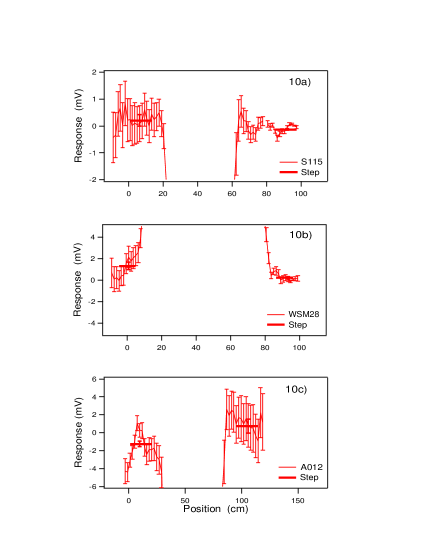
Figure 18: Steps: D0 Al, CDF Pb, and CDF Al.

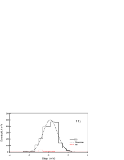
Figure 19: Steps from D0 samples. A Dirac pole would appear as a step at 2.46 mV.

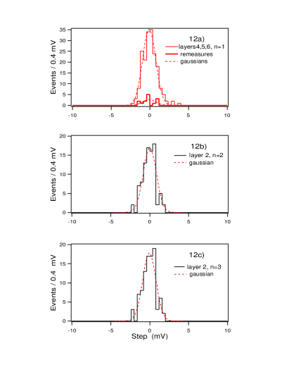
Figure 20: Steps from CDF Pb samples. A Dirac pole would appear as a step at 2.46 mV.

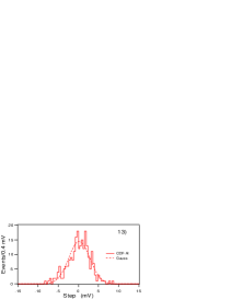
Figure 21: Steps from CDF Al samples. A Schwinger pole ($2g_{D}$) would appear as a step at 10.64 mV.

For $m^{\prime}=1/2$ the 90% confidence upper limit is 4.2 signal events for 8 events observed when 10 were expected [205]. These 8 samples were remeasured and all fell within $\pm 1.47$ mV of $m^{\prime}=0$. (More than 1.28$\sigma$ from $|m^{\prime}|=1/2$.) For $m^{\prime}=1$ the 90% confidence upper limit is 2.4 signal events for zero events observed and zero expected.

By putting in angular and mass acceptances we can get cross section limits as shown in table 2.

Table 2: Alternative interpretations for different production angular distributions of the monopoles, comparing $1$ and $1\pm\cos^{2}\theta$. Here the cross section $\sigma_{a}$ corresponds to the distribution $1+a\cos^{2}\theta$, and similarly for the mass limits (all at 90% confidence level).

• Set	$2m^{\prime}$	$\sigma^{\rm ul}_{+1}$	$m^{\rm LL}_{+1}$	$\sigma^{\rm ul}_{0}$	$m^{\rm LL}_{0}$	$\sigma^{\rm ul}_{-1}$	$m^{\rm LL}_{-1}$
  		(pb)	(GeV/$c^{2}$)	(pb)	(GeV/$c^{2}$)	(pb)	(GeV/$c^{2}$)
  1 Al	1	1.2	250	1.2	240	1.4	220
  1 Al RM	1	0.6	275	0.6	265	0.7	245
  2 Pb	1	9.9	180	12	165	23	135
  2 Pb RM	1	2.4	225	2.9	210	5.9	175
  1 Al	2	2.1	280	2.2	270	2.5	250
  2 Pb	2	1.0	305	0.9	295	1.1	280
  3 Al	2	0.2	365	0.2	355	0.2	340
  1 Be	3	3.9	285	5.6	265	47	180
  2 Pb	3	0.5	350	0.5	345	0.5	330
  3 Al	3	0.07	420	0.07	410	0.06	405
  1 Be	6	1.1	330	1.7	305	18	210
  3 Al	6	0.2	380	0.2	375	0.2	370

These numbers reflect the new analysis, published in 2004 [21], and so differ somewhat from our earlier published results [20]. To obtain the mass limits, we use the model cross sections given in figure 22.

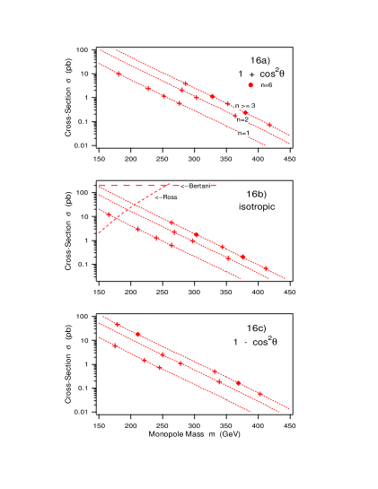
Figure 22: Cross section vs. mass limits. The three graphs show three different assumptions about the angular distribution, since even if we knew the spin of the monopole, we cannot at present predict the differential cross section. Shown in the second figure are the Bertani [167] and lunar [25] limits.

Finally, we show in figure 23 what might be achievable at the LHC, using the same techniques applied here.

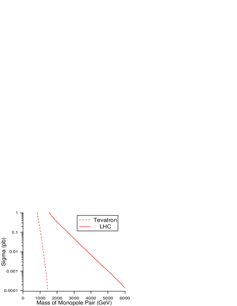
Figure 23: Monopole pair masses as a function of the cross section at the Tevatron ($p\bar{p}$ at 2 TeV) and at the LHC ($pp$ at 14 TeV). Both include the $\beta^{3}$ correction, and are for a Dirac monopole, $m^{\prime}=1/2$.

12 H1 limits

We now turn to the limits on monopole production obtained from $e^{+}p$ collisions at HERA recently published by the H1 collaboration [206]. This production mechanism is intermediate between that of $p\bar{p}$ experiments such as that given in [21], and that of the possible production through $e^{+}e^{-}$ collisions [182], and conceivably might yield a cleaner interpretation if monopole condensates are responsible for the confinement of quarks [15, 207, 208, 209]. Although the mass limits determined are not as strong as in our experiment described in the previous section, it is crucial that different physical domains be explored carefully.

In their experiment, the aluminum beam pipe used at the H1 interaction point at HERA during 1995–1997 was cut into 75 long and short strips. This beam pipe had been exposed to an integrated luminosity of $62\pm 1$ pb^-1. These strips were then placed on a conveyor belt and passed through a warm-bore magnetometer at Southhampton Oceanographic Centre, UK. If a monopole passed through the superconducting coil, as in our experiment, it would establish a persistent current there, which would be detected by a SQUID. Again they calibrated their detector by a long, thin solenoid, which at each end produced a pseudopole. Calibration was within some 10% for pole strengths above $g_{D}=\hbar c/2e$. Large dipole signals were seen, but the signals always returned to the baseline unless a pseudopole was present. A few persistent current events were seen, but they always disappeared upon remeasurement. Some of the runs exhibited large fluctuations of unknown orgin, but none was consistent with a monopole event.

No monopole was detected in their experiment of strength greater than $0.1g_{D}$ for a sample consisting of $93\pm 3\%$ of the beam pipe. To interpret this as a limit on the production cross section, models had to be adopted, since perturbation theory was unreliable. Two models were tried:

$$e^{+}p\to e^{+}M\bar{M}p,\qquad\mbox{spin 0 monopole},$$ (2.2difgknopsacaeanbgbncdcecodgdxdzcfkvaaacakbbbhbqbvbycacdcedlefijbknaa)

$$e^{+}p\to e^{+}M\bar{M}X,\qquad\mbox{spin 1/2 monopole},$$ (2.2difgknopsacaeanbgbncdcecodgdxdzcfkvaaacakbbbhbqbvbycacdcedlefijbknab)

where in both models the monopole pairs were produced by two-photon processes. The effects on the produced monopoles by the H1 magnetic fields were included. The stopping power was computed by using the classical results of Ahlen [210, 203, 132].

The results of their analysis are expressed in plots of the upper limits on the cross sections for a given monopole mass, up to a mass of 140 GeV, for different models and magnetic charges. That is, cross sections above those limits are excluded based on their experimental analysis. These limits are weakest for the Dirac charge, $g_{D}$, and strongest for Schwinger quantization based on quark charges, $6g_{D}$, of course. For model (2.2difgknopsacaeanbgbncdcecodgdxdzcfkvaaacakbbbhbqbvbycacdcedlefijbknaa) the cross section limits range from about 1 pb for several GeV to more that 100 pb for 140 GeV for $g_{D}$. For higher charges the limits are relatively constant around 0.1 pb or less. For (2.2difgknopsacaeanbgbncdcecodgdxdzcfkvaaacakbbbhbqbvbycacdcedlefijbknab) the limits are similar, except for $g_{D}$, where the limit drops below 0.1 pb for 10 GeV masses or less. Thus their results our complementary to ours: Our mass limits are stronger, but in some cases they reach smaller cross sections for lower masses.

13 CDF limits

Quite recently, a new CDF experiment [168] has been announced, which claims, on the basis of an integrated luminosity of 35.7 pb^-1, a production cross section limit for spin-1/2 monopoles below 0.2 pb for masses between 200 and 700 GeV, and hence, in a Drell-Yan model, a lower mass limit of 360 GeV. (These limits are quoted at the 95% confidence level.) This is based on quite different technology than the Oklahoma or H1 experiments. Rather, they looked at a sample of $p\bar{p}$ events collected during 2003 by the CDF detector by a special trigger. The signal for a monopole is the large ionization and heavy production of delta rays by such a particle. They use our crude model of replacing $e$ by $g\beta$ in the Drell-Yan production mechanism [20, 21], apart from this simply replacing the lepton mass by the monopole mass. Acceptance is affected by production kinematics, which effect they estimate at 10%. Light monopoles will be swept out of the detector by the magnetic field, while heavy monopoles may reach the time-of-flight detector too late to cause a trigger. Other particles (“spoilers”) may cause a charge integration to start in the detector before a monopole signal arrives; they estimate a few percent fraction for a monopole of mass 400 GeV.

Out of 130,000 candidate events, no monopole trigger events were found, from which the limit quoted above was extracted. They believe they can push the limit on masses up another 100 GeV with additional Run II data.

13.1 Comments on CDF experiment

One might ask how can CDF claim stronger limits than we do based on less than 1/4 of the integrated luminosity of our experiment. The answer, I believe, is that our experimental limit is extremely conservative. They may have underestimated the systematic effect of huge uncertainties in the production mechanism, while at the same time they claim our limit is dependent on the trapping model, which it is not. Undoubtedly, the $\rmd E/\rmd x$ signature of monopoles is much less well understood than the clear-cut electromagnetic signature of an induction detector. This is not to denigrate the utility of this measurement, but to emphasize that the limits so obtained are subject to large, relatively uncontrolled, uncertainties.

14 Conclusions

One magnetic monopole, carrying magnetic charge $g$, will result in the quantization of electric charge throughout the universe,

$$e=\frac{m^{\prime}\hbar c}{g},$$ (2.2difgknopsacaeanbgbncdcecodgdxdzcfkvaaacakbbbhbqbvbycacdcedlefijbknaa)

where $m^{\prime}$ is a half-integer,

$$m^{\prime}=0,\pm\frac{1}{2},\pm 1,\pm\frac{3}{2},\pm 2,\pm\frac{5}{2},\dots.$$ (2.2difgknopsacaeanbgbncdcecodgdxdzcfkvaaacakbbbhbqbvbycacdcedlefijbknab)

That electric charge is quantized in integer multiples of the electron charge (or integer multiples of the quark charge) is an overwhelming fact, which does not possess a simple explanation. This, perhaps, is the most compelling argument in favor of the existence of magnetic charge. A second argument is the greater symmetry (duality) imparted to Maxwell’s equations, and to classical and quantum electrodynamics, if both electric and magnetic charges are present. Thus from phenomenological and theoretical bases, the arguments in favor of the existence of magnetic charge and for dual QED are at least as strong as those for supersymmetry. Unfortunately, like for the latter, there is not a real shred of observational evidence in favor of magnetic charge, although here it is far less embarrassing to be in that situation, since the most likely mass range for magnetically charged particles is not far from the Planck scale.

In this review we have concentrated on the theory of point Dirac monopoles or Schwinger dyons, starting from the classical scattering, through the nonrelativistic quantum mechanical description, to the quantum field theory of such objects. For lack of space we have only briefly referred to the classical monopoles that arise from the solution of non-Abelian gauge theories. From the point of view of phenomenology and the setting of experimental limits, the point description should be adequate, since the structure of composite monopoles only emerges at the energy scale that sets the mass of the particles. (An exception, of course, occurs with limits based on that structure, such as the catalysis of proton decay.) In addition, our concern has been chiefly with the quantum description, which has been only roughly sketched for composite monopoles.

We close, as did Schwinger in his provocative article [11], by quoting from Faraday: “Nothing is too wonderful to be true, if it be consistent with the laws of nature, and in such things as these, experiment is the best test of such consistency.”

References

References

- [1] May 28, 2005. http://www.languagehat.com/archives/001914.php.
- [2] Pierre de Maricourt. On the Magnet, letter to Siger de Foucaucourt, (1269). In The Letter of Petrus Peregrinus on the Magnet, New York, 1904. McGraw-Hill. Translated by Brother Arnold.
- [3] H. Poincaré. Remarques sur une expérience de M. Birkeland. Compt. Rendus, 123:530, 1896.
- [4] J. J. Thomson. Electricity and Matter. Scribners, New York, 1904. Lectures given at Yale University.
- [5] J. J. Thomson. On momentum in the electric field. Philos. Mag., 8:331–356, 1904.
- [6] M. Faraday. Experimental Researches in Electricity. Taylor, London, 1844.
- [7] O. Heaviside. Electromagnetic Theory, volume 1. Benn, London, 1893.
- [8] P. Curie. On the possible existence of magnetic conductivity and free magnetism. Sèances Soc. Phys. (Paris), pages 76–77, 1894.
- [9] P. A. M. Dirac. Quantised singularities in the electromagnetic field. Proc. Roy. Soc. Lond., A133:60–72, 1931.
- [10] R. Kane. Erkenntnis, 24:115, 1986.
- [11] J. Schwinger. A magnetic model of matter. Science, 165:757–761, 1969.
- [12] T. T. Wu and C. N. Yang. Some solutions of the classical isotopic gauge field equations. In H. Mark and S. Fernbach, editors, Properties of Matter Under Unusual Conditions, page 349, New York, 1969. Wiley.
- [13] G. ’t Hooft. Magnetic monopoles in unified gauge theories. Nucl. Phys., B79:276–284, 1974.
- [14] A. M. Polyakov. Particle spectrum in quantum field theory. JETP Lett., 20:194–195, 1974. [Pisma Zh. Eksp. Teor. Fiz. 20:430-433,1974].
- [15] Y. Nambu. Strings, monopoles, and gauge fields. Phys. Rev. D, 10:4262, 1974.
- [16] B. Julia and A. Zee. Poles with both magnetic and electric charges in nonabelian gauge theory. Phys. Rev., D11:2227–2232, 1975.
- [17] T. T. Wu and C. N. Yang. Some remarks about unquantized nonabelian gauge fields. Phys. Rev., D12:3843–3844, 1975.
- [18] A. S. Goldhaber and W. P. Trower. Resource letter MM1: Magnetic monopoles. Am. J. Phys., 58:429, 1990.
- [19] J. Schwinger, K. A. Milton, W.-y. Tsai, L. L. DeRaad, Jr., and D. C. Clark. Nonrelativistic dyon dyon scattering. Ann. Phys. (N.Y.), 101:451, 1976.
- [20] G. R. Kalbfleisch et al. Improved experimental limits on the production of magnetic monopoles. Phys. Rev. Lett., 85:5292–5295, 2000.
- [21] G. R. Kalbfleisch, W. Luo, K. A. Milton, E. H. Smith, and M. G. Strauss. Limits on production of magnetic monopoles utilizing samples from the D0 and CDF detectors at the Tevatron. Phys. Rev., D69:052002, 2004.
- [22] L. W. Alvarez. Design of an electromagnetic detector for Dirac monopoles. 1963. UCRL-AGM-470.
- [23] L. W. Alvarez, P. H. Eberhard, R. R. Ross, and R. D. Watt. Search for magnetic monopoles in the lunar sample. Science, 167:701–703, 1970.
- [24] P. H. Eberhard, R. R. Ross, L. W. Alvarez, and R. D. Watt. Search for magnetic monopoles in lunar material. Phys. Rev., D4:3260, 1971.
- [25] R. R. Ross, P. H. Eberhard, L. W. Alvarez, and R. D. Watt. Search for magnetic monopoles in lunar material using an electromagnetic detector. Phys. Rev., D8:698, 1973.
- [26] P. H. Eberhard, R. R Ross, J. D. Taylor, L. W. Alvarez, and H. Oberlack. Evidence at the probability level against the production of magnetic monopoles in proton interactions at 300 GeV/c. Phys. Rev., D11:3099–3104, 1975.
- [27] J. Schwinger, L. L. DeRaad, Jr., K. A. Milton, and W.-y. Tsai. Classical Electrodynamics. Perseus Books/Westview Press, New York, 1998.
- [28] H. A. Bethe. Theory of diffraction by small holes. Phys. Rev., 66:163, 1944.
- [29] K. A. Milton and J. Schwinger. Electromagnetic Radiation: Variational Methods, Waveguides, and Acclerators. Springer-Verlag, Berlin, 2006.
- [30] J. J. Thomson. Elements of the Mathematical Theory of Electricity and Magnetism. Cambridge University Press, Cambridge, 4th edition, 1909.
- [31] J. J. Thomson. Recollections and Reflections. Macmillan, New York, 1937.
- [32] M. Birkeland. Sur un spectre des rayons cathodiques. Compt. Rendus, 123:492, 1896.
- [33] J. Schwinger. Magnetic charge and the charge quantization condition. Phys. Rev., D12:3105, 1975.
- [34] T. T. Wu and C. N. Yang. Dirac’s monopole without strings: Classical Lagrangian theory. Phys. Rev., D14:437–445, 1976.
- [35] T. T. Wu and C. N. Yang. Dirac monopole without strings: Monopole harmonics. Nucl. Phys., B107:365, 1976.
- [36] Y. Kazama and C. N. Yang. Existence of bound states for a charged spin-1/2 particle with an extra magnetic moment in the field of a fixed magnetic monopole. Phys. Rev., D15:2300, 1977.
- [37] T. T. Wu and C. N. Yang. Some properties of monopole harmonics. Phys. Rev., D16:1018–1021, 1977.
- [38] C. N. Yang. Generalization of Dirac’s monopole to SU(2) gauge fields. J. Math. Phys., 19:320, 1978.
- [39] Y. Kazama, C. N. Yang, and A. S. Goldhaber. Scattering of a Dirac particle with charge by a fixed magnetic monopole. Phys. Rev., D15:2287, 1977.
- [40] C. N. Yang. SU(2) monopole harmonics. J. Math. Phys., 19:2622, 1978.
- [41] C. N. Yang. Fiber bundles and the physics of the magnetic monopole. Presented at Chern Symposium, Berkeley, Calif., Jun 1979.
- [42] A. S. Goldhaber. Role of spin in the monopole problem. Phys. Rev., 140:B1407, 1965.
- [43] A. S. Goldhaber. Dirac particle in a magnetic field: Symmetries and their breaking by monopole singularities. Phys. Rev., D16:1815, 1977.
- [44] K. A. Milton and L. L. DeRaad, Jr. Strings and gauge invariance. J. Math. Phys., 19:375, 1978.
- [45] B. Zumino. In A. Zichichi, editor, Strong and Weak Interactions–Present Problems, page 771, New York. Academic.
- [46] D. G. Boulware, L. S. Brown, R. N. Cahn, S. D. Ellis, and C.-k. Lee. Scattering on magnetic charge. Phys. Rev., D14:2708, 1976.
- [47] T. T. Wu and C. N. Yang. Concept of nonintegrable phase factors and global formulation of gauge fields. Phys. Rev. D, 12:3845, 1975.
- [48] C. N. Yang. In Proceedings of the Sixth Hawaii Topical Conference on Particle Physics, Honolulu, 1976. University of Hawaii.
- [49] T. M. Yan. Classical theory of magnetic charge. Phys. Rev., 160:1182, 1967.
- [50] R. A. Brandt and J. R. Primack. Avoiding ‘Dirac’s veto’ in monopole theory. Phys. Rev., D15:1798–1802, 1977.
- [51] R. A. Brandt and J. R. Primack. Moving and removing Dirac’s string. Phys. Rev., D15:1175, 1977.
- [52] C. A. Hurst. Charge quantization and nonintegrable Lie algebra. Ann. Phys. (N.Y.), 50:51, 1968.
- [53] H. J. Lipkin, W. I. Weisberger, and M. Peshkin. Magnetic charge quantization and angular momentum. Ann. Phys. (N.Y.), 53:203, 1969.
- [54] J. Tamm. Die verallgemeinerten kugelfunktionen und die wellenfunktionen eines electrons un feld eines magnetpoles. Z. Phys., 71:141–150, 1931.
- [55] P. Banderet. On the theory of a point magnetic pole. Helv. Phys. Acta, 19:503, 1946.
- [56] M. Fierz. On the theory of particles with magnetic charge. Helv. Phys. Acta, 17:27–34, 1944.
- [57] K. Ford and J. A. Wheeler. Application of semiclassical scattering analysis. Ann. Phys. (N.Y.), 7:287, 1959.
- [58] I. R. Lapidus and J. L. Pietenpol. Classical interaction of an electric charge with a magnetic monopole. Am. J. Phys., 28:17–18, 1960.
- [59] G. Nadeau. Concerning the classical interaction of an electric charge with a magnetic monopole. Am. J. Phys., 28:566, 1960.
- [60] M. K. Prasad and C. M. Sommerfield. An exact classical solution for the ’t Hooft monopole and the Julia-Zee dyon. Phys. Rev. Lett., 35:760–762, 1975.
- [61] E. B. Bogomolny. Stability of classical solutions. Sov. J. Nucl. Phys., 24:449, 1976.
- [62] H. Georgi and S. L. Glashow. Unified weak and electromagnetic interactions without neutral currents. Phys. Rev. Lett., 28:1494, 1972.
- [63] J. Preskill. Magnetic monopoles. Ann. Rev. Nucl. Part. Sci., 34:461–530, 1984.
- [64] T. W. Kirkman and C. K. Zachos. Asymptotic analysis of the monopole structure. Phys. Rev., D24:999, 1981.
- [65] S. Coleman. In A. Zichichi, editor, The Unity of Fundamental Interactions, New York. Plenum.
- [66] Y. M. Cho and D. Maison. Monopole configuration in Weinberg-Salam model. Phys. Lett., B391:360–365, 1997. hep-th/9601028.
- [67] Y. M. Cho and K. Kimm. Finite energy electroweak monopoles. 1997. hep-th/9707038.
- [68] Y. M. Cho and K. Kimm. Electroweak monopoles. 1997. hep-th/9705213.
- [69] E. J. Weinberg. Fundamental monopoles in theories with arbitrary symmetry breaking. Nucl. Phys., B203:445, 1982.
- [70] A. Rajantie. Mass of a quantum ’t Hooft-Polyakov monopole. 2005. hep-lat/0512006.
- [71] P. M. Sutcliffe. BPS monopoles. Int. J. Mod. Phys., A12:4663–4706, 1997.
- [72] N. S. Manton and P. Sutcliffe. Topological Solitons. Cambridge University Press, 2004.
- [73] M. P. Nair. Quantum Field Theory: A Modern Perspective. Springer, New York, 2005.
- [74] A. Khvedelidze, A. Kovner, and D. McMullan. Magnetic monopoles in : A perturbative calculation. 2005. hep-th/0512142.
- [75] J. Schwinger. Magnetic charge and quantum field theory. Phys. Rev., 144:1087–1093, 1966.
- [76] J. Schwinger. Electric and magnetic-charge renormalization. I. Phys. Rev., 151:1048, 1966.
- [77] J. Schwinger. Electric and magnetic-charge renormalization. II. Phys. Rev., 151:1055, 1966.
- [78] J. Schwinger. Sources and magnetic charge. Phys. Rev., 173:1536–1544, 1968.
- [79] D. Zwanziger. Quantum field theory of particles with both electric and magnetic charges. Phys. Rev., 176:1489–1495, 1968.
- [80] D. Zwanziger. Local Lagrangian quantum field theory of electric and magnetic charges. Phys. Rev., D3:880, 1971.
- [81] R. A. Brandt, F. Neri, and D. Zwanziger. Lorentz invariance of the quantum field theory of electric and magnetic charge. Phys. Rev. Lett., 40:147, 1978.
- [82] R. Brandt, F. Neri, and D. Zwanziger. Phys. Rev. D, 19:1153, 1979.
- [83] Blagojević, M. and Senjanović, P. The quantum field theory of electric and magnetic charge. Phys. Rept., 157:233, 1988.
- [84] L. P. Gamberg and K. A. Milton. Dual quantum electrodynamics: Dyon-dyon and charge-monopole scattering in a high-energy approximation. Phys. Rev., D61:075013, 2000.
- [85] P. A. M. Dirac. The theory of magnetic poles. Phys. Rev., 74:817–830, 1948.
- [86] J. Schwinger. Particles, Sources, and Fields, volume 1. Addison-Wesley, New York, 1970. republished by Perseus Books, 1998.
- [87] P. A. M. Dirac. Can. J. Phys., 33:650, 1955.
- [88] A. N. Sisakyan, N. B. Skachkov, I. L. Solovtsov, and O. Yu. Shevchenko. Gauge invariant approach and infrared behavior of spinor propagator. Theor. Math. Phys., 78:185, 1989. [Teor. Mat. Fiz. 78:258-266, 1989].
- [89] W. Deans. Quantum field theory of Dirac monopoles and the charge quantization condition. Nucl. Phys., B197:307, 1982.
- [90] J. Schwinger. On the Green’s functions of quantized fields. 1. Proc. Nat. Acad. Sci., 37:452–455, 1951.
- [91] J. Schwinger. On the Green’s functions of quantized fields. 2. Proc. Nat. Acad. Sci., 37:455–459, 1951.
- [92] S. Mandelstam. Quantum electrodynamics without potentials. Ann. Phys., 19:1–24, 1962.
- [93] B. Zumino. Gauge properties of propagators in quantum electrodynamics. J. Math. Phys., 1:1–7, 1960.
- [94] I. Bialynicki-Birula. On the gauge covariance of quantum electrodynamics. J. Math. Phys., 3:1094, 1962.
- [95] J. Zinn-Justin. Quantum Field Theory and Critical Phenomena. Oxford University Press, Oxford, 3rd edition, 1996.
- [96] J. Schwinger. Brownian motion of a quantum oscillator. J. Math. Phys., 2:407–432, 1961.
- [97] C. Sommerfield. On the definition of currents and the action principle in field theories of one spatial dimension. Ann. Phys. (NY), 26:1, 1963.
- [98] K. Johnson. In S. Deser and K. Ford, editors, Lectures on Particles and Field Theory, page 1, Englewood Cliffs, 1965. Prentice-Hall.
- [99] K. Symanzik. Z. Naturforsch., 9A:809, 1954.
- [100] H. M. Fried. Functional Methods and Eikonal Models. Editions Frontières, Gif-sur-Yvette Cedex, 1990.
- [101] O. Nachtmann. Considerations concerning diffraction scattering in quantum chromodynamics. Ann. Phys. (N.Y.), 209:436–478, 1991.
- [102] G. P. Korchemsky. On near forward high-energy scattering in QCD. Phys. Lett., B325:459–466, 1994.
- [103] I. A. Korchemskaya and G. P. Korchemsky. High-energy scattering in QCD and cross singularities of wilson loops. Nucl. Phys., B437:127–162, 1995.
- [104] G. C. Gellas, A. I. Karanikas, and C. N. Ktorides. Worldline approach to eikonals for QED and linearized quantum gravity and their off mass shell extensions. Phys. Rev., D57:3763–3776, 1998.
- [105] A. I. Karanikas and C. N. Ktorides. Worldline approach to forward and fixed angle fermion fermion scattering in Yang-Mills theories at high energies. Phys. Rev., D59:016003, 1999.
- [106] M. Quiros. An eikonal expansion in quantum electrodynamics. Helv. Phys. Acta, 49:849–862, 1976.
- [107] H. M. Fried and Y. Gabellini. Non-Abelian eikonals. Phys. Rev., D55:2430–2440, 1997.
- [108] F. Bloch and A. Nordsieck. Note on the radiation field of the electron. Phys. Rev., 52:54–59, 1937.
- [109] G. W. Erickson and H. M. Fried. Lepton scattering amplitudes in two model field theories. J. Math. Phys., 6:414, 1965.
- [110] H. M. Fried. Construction of a complete eikonal representation. Phys. Rev., D3:2010–2013, 1971.
- [111] M. Levy and J. Sucher. Eikonal approximation in quantum field theory. Phys. Rev., 186:1656–1670, 1969.
- [112] M. Levy and J. Sucher. Asymptotic behavior of scattering amplitudes in the relativistic eikonal approximation. Phys. Rev., D2:1716–1723, 1970.
- [113] H. D. I. Abarbanel and C. Itzykson. Relativistic eikonal expansion. Phys. Rev. Lett., 23:53, 1969.
- [114] W. Dittrich. Equivalence of the Dirac equation to a subclass of Feynman diagrams. Phys. Rev., D1:3345–3348, 1970.
- [115] W. Dittrich. Relativistic eikonal propagators and high-energy scattering in QED. Nucl. Phys., B45:290–302, 1972.
- [116] K. Gottfried. Quantum Mechanics. Addison-Wesley, Reading, Massachusetts, 1966.
- [117] C. Itzykson and J. B. Zuber. Quantum Field Theory. McGraw-Hill, New York, 1980.
- [118] L. F. Urrutia. Zeroth order eikonal approximation in relativistic charged particle-monopole scattering. Phys. Rev., D18:3031, 1978.
- [119] Ore, F. R., Jr. Lorentz invariance of charge-monopole scattering. Phys. Rev., D13:2295, 1976.
- [120] H. M. Fried and Y. M. Gabellini. Phase averaging and generalized eikonal representations. Phys. Rev., D51:890–905, 1995.
- [121] H. M. Fried and Y. M. Gabellini. Special variant of the Fradkin representation. Phys. Rev., D51:906–918, 1995.
- [122] H. M. Fried, Y. Gabellini, and B. H. J. McKellar. Exact and approximate fermion Green’s functions in QED and QCD. Phys. Rev., D51:7083–7096, 1995.
- [123] E. S. Fradkin. Application of functional methods in quantum field theory and quantum statistics (ii). Nucl. Phys., 76:588, 1966.
- [124] K. V. Shajesh and K. A. Milton. Quantum mechanics using Fradkin’s representation. 2005. hep-th/0510103.
- [125] L. V. Laperashvili and H. B. Nielsen. Dirac relation and renormalization group equations for electric and magnetic fine structure constants. Mod. Phys. Lett., A14:2797, 1999.
- [126] L. V. Laperashvili and H. B. Nielsen. Phase transition in the Higgs model of scalar fields with electric and magnetic charges. Int. J. Mod. Phys., A16:2365–2390, 2001.
- [127] L. V. Laperashvili, D. A. Ryzhikh, and H. B. Nielsen. Monopoles near the Planck scale and unification. Int. J. Mod. Phys., A18:4403–4442, 2003.
- [128] L. V. Laperashvili, H. B. Nielsen, and D. A. Ryzhikh. Monopoles and family replicated unification. Phys. Atom. Nucl., 66:2070–2077, 2003.
- [129] C. R. Das, L. V. Laperashvili, and H. B. Nielsen. Generalized dual symmetry of nonabelian theories, monopoles and dyons. 2005.
- [130] L. Gamberg, G. R. Kalbfleisch, and K. A. Milton. Direct and indirect searches for low mass magnetic monopoles. Found. Phys., 30:543, 2000.
- [131] S. Eidelman et al. Review of Particle Physics. Physics Letters B, 592:1+, 2004. http://pdg.lbl.gov.
- [132] S. P. Ahlen and K. Kinoshita. Calculation of the stopping power of very low velocity magnetic monopoles. Phys. Rev., D26:2347–2363, 1982.
- [133] S. P. Ahlen. Monopole energy loss and detector excitation mechanisms. In R. A. Carrigan and W. P. Trower, editors, Magnetic Monopoles, pages 259–290, New York, 1982. Plenum Press. Wingspread 1982.
- [134] W. Luo. Search for magnetic monopoles possibly produced by proton- antiproton collisions at the Tevatron collider. PhD thesis, University of Oklahoma, 2002. UMI-30-56946 (AAT 3056946).
- [135] P. Osland and T. T. Wu. Monopole-fermion and dyon-fermion bound states. 1. General properties and numerical results. Nucl. Phys., B247:421, 1984.
- [136] P. Osland and T. T. Wu. Monopole-fermion and dyon-fermion bound states. 2. Weakly bound states for the lowest angular momentum. Nucl. Phys., B247:450, 1984.
- [137] P. Osland and T. T. Wu. Monopole-fermion and dyon-fermion bound states. 3. Monopole-fermion system with and large . Nucl. Phys., B256:13, 1985.
- [138] P. Osland and T. T. Wu. Monopole-fermion and dyon-fermion bound states. 4. Dyon-fermion system with and large . Nucl. Phys., B256:32, 1985.
- [139] P. Osland, C. L. Schultz, and T. T. Wu. Monopole-fermion and dyon-fermion bound states. 5. Weakly bound states for the monopole-fermion system. Nucl. Phys., B256:449, 1985.
- [140] P. Osland and T. T. Wu. Monopole-fermion and dyon-fermion bound states. 6. Weakly bound states for the dyon-fermion system. Nucl. Phys., B261:687, 1985.
- [141] W. van R. Malkus. The interaction of the Dirac magnetic monopole with matter. Phys. Rev., 83:899–905, 1951.
- [142] L. Bracci and G. Fiorentini. Interactions of magnetic monopoles with nuclei and atoms: Formation of bound states and phenomenological consequences. Nucl. Phys., B232:236, 1984.
- [143] L. Bracci, G. Fiorentini, and R. Tripiccione. On the energy loss of very slowly moving magnetic monopoles. Nucl. Phys., B238:167, 1984.
- [144] L. Bracci, G. Fiorentini, G. Mezzorani, and P. Quarati. Formation of monopole-proton bound states in the hot universe. Phys. Lett., B143:357, 1984. Erratum B155, 468 (1985).
- [145] L. Bracci and G. Fiorentini. On the capture of protons by magnetic monopoles. Nucl. Phys., B249:519, 1985.
- [146] D. W. Sivers. Possible binding of a magnetic monopole to a particle with electric charge and a magnetic dipole moment. Phys. Rev., D2:2048–2054, 1970.
- [147] K. Olaussen and R. Sollie. Form-factor effects on nucleus-magnetic monopole binding. Nucl. Phys., B255:465, 1985.
- [148] K. Olaussen, H. A. Olsen, P. Osland, and I. Overbo. Kazama-Yang monopole-fermion bound states. 1. Analytic results. Nucl. Phys., B228:567, 1983.
- [149] K. Olaussen, H. A. Olsen, I. Overbo, and P. Osland. Proton capture by magnetic monopoles. Phys. Rev. Lett., 52:325, 1984.
- [150] T. F. Walsh, P. Weisz, and T. T. Wu. Monopole catalysis of proton decay. Nucl. Phys., B232:349, 1984.
- [151] H. A. Olsen, P. Osland, and T. T. Wu. On the existence of bound states for a massive spin 1 particle and a magnetic monopole. Phys. Rev., D42:665–689, 1990.
- [152] H. A. Olsen and P. Osland. Bound states for a massive spin 1 particle and a magnetic monopole. Phys. Rev., D42:690–700, 1990.
- [153] C. J. Goebel. Binding of nuclei to monopoles. In J. L. Stone, editor, Monopole ’83, page 333, New York, 1984. Plenum. MAD/TH/146.
- [154] E. Goto, H. Kolm, and K. Ford. Search for ferromagnetically trapped magnetic monopoles of cosmic-ray origin. Phys. Rev., 132:387, 1963.
- [155] R. A. Carrigan, Jr., B. P. Strauss, and G. Giacomelli. Search for magnetic monopoles at the CERN ISR. Phys. Rev., D17:1754, 1978.
- [156] M. Turner. Thermal production of superheavy magnetic monopoles in the early universe. Phys. Lett., B115:95, 1982.
- [157] P. B. Price, S. l. Guo, S. P. Ahlen, and R. L. Fleischer. Search for grand unified theory magnetic monopoles at a flux level below the Parker limit. Phys. Rev. Lett., 52:1265, 1984.
- [158] B. Cabrera. First results from a superconductive detector for moving magnetic monopoles. Phys. Rev. Lett., 48:1378, 1982.
- [159] B. Cabrera. Upper limit on flux of cosmic ray monopoles obtained with a three loop superconductive detector. Phys. Rev. Lett., 51:1933, 1983.
- [160] H. Jeon and M. J. Longo. Search for magnetic monopoles trapped in matter. Phys. Rev. Lett., 75:1443–1446, 1995.
- [161] H. Jeon and M. J. Longo. Search for magnetic monopoles trapped in matter. Phys. Rev. Lett., 76:159, 1996. Erratum.
- [162] M. Ambrosio et al. Magnetic monopole search with the MACRO detector at Gran Sasso. Phys. Lett., B406:249, 1997.
- [163] P. B. Price, E. K. Shirk, W. Z. Osborne, and L. S. Pinsky. Evidence for detection of a moving magnetic monopole. Phys. Rev. Lett., 35:487–490, 1975.
- [164] L. W. Alvarez. Analysis of a reported magnetic monopole. In Int. Conf. on Lepton and Photon Interactions, Stanford, 1975.
- [165] G. Giacomelli and L. Patrizii. Magnetic monopole searches. 2003. hep-ex/0302011.
- [166] G. Giacomelli and L. Patrizii. Magnetic monopole searches. 2005. hep-ex/0506014.
- [167] M. Bertani et al. Search for magnetic monopoles at the Tevatron collider. Europhys. Lett., 12:613–616, 1990.
- [168] A. Abulencia et al. Direct search for Dirac magnetic monopoles in collisions at TeV. 2005.
- [169] G. Giacomelli. Magnetic monopoles. Riv. Nuovo Cim., 7N12:1–111, 1984.
- [170] J. Preskill. Cosmological production of superheavy magnetic monopoles. Phys. Rev. Lett., 43:1365, 1979.
- [171] M. S. Turner, E. N. Parker, and T. J. Bogdan. Magnetic monopoles and the survival of galactic magnetic fields. Phys. Rev., D26:1296, 1982.
- [172] E. N. Parker. The origin of magnetic fields. Astrophys. J., 160:383, 1970.
- [173] V. A. Rubakov. Superheavy magnetic monopoles and proton decay. JETP Lett., 33:644–646, 1981.
- [174] C. G. Callan, Jr. Dyon-fermion dynamics. Phys. Rev., D26:2058–2068, 1982.
- [175] M. Ambrosio et al. Search for nucleon decays induced by GUT magnetic monopoles with the MACRO experiment. Eur. Phys. J., C26:163–172, 2002.
- [176] M. Ambrosio et al. Final results of magnetic monopole searches with the MACRO experiment. Eur. Phys. J., C25:511–522, 2002.
- [177] P. B. Price. Limits on contribution of cosmic nuclearites to galactic dark matter. Phys. Rev., D38:3813–3814, 1988.
- [178] D. Ghosh and S. Chatterjea. Supermassive magnetic monopoles flux from the oldest mica samples. Europhys. Lett., 12:25–28, 1990.
- [179] G. Lazarides, C. Panagiotakopoulos, and Q. Shafi. Magnetic monopoles from superstring models. Phys. Rev. Lett., 58:1707, 1987.
- [180] T. W. Kephart and Q. Shafi. Family unification, exotic states and magnetic monopoles. Phys. Lett., B520:313–316, 2001.
- [181] A. De Rujúla. Effects of virtual monopoles. Nucl. Phys., B435:257–276, 1995.
- [182] M. Acciarri et al. Search for anomalous events at LEP. Phys. Lett., B345:609, 1995.
- [183] I. F. Ginzburg and S. L. Panfil. The possibility of observation of heavy Dirac-Schwinger magnetic pole. Sov. J. Nucl. Phys., 36:850, 1982.
- [184] I. F. Ginzburg and A. Schiller. Search for a heavy magnetic monopole at the Tevatron and LHC. Phys. Rev., D57:6599–6603, 1998.
- [185] I. F. Ginzburg and A. Schiller. The visible effect of a very heavy magnetic monopole at colliders. Phys. Rev., D60:075016, 1999.
- [186] B. Abbott et al. A search for heavy pointlike Dirac monopoles. Phys. Rev. Lett., 81:524–529, 1998.
- [187] S. Graf, A. Schaefer, and W. Greiner. Mass limit for Dirac-type magnetic monopoles. Phys. Lett., B262:463–466, 1991.
- [188] W. Heisenberg and H. Euler. Consequences of Dirac’s theory of positrons. Z. Phys., 98:714–732, 1936.
- [189] V. Weisskopf. Kgl. Danske Videnskab. Selskabs. Mat.-fys. Medd., 14(6), 1936.
- [190] J. Schwinger. On gauge invariance and vacuum polarization. Phys. Rev., 82:664–679, 1951.
- [191] J. Schwinger. Particles, Sources, and Fields, volume 2. Addison-Wesley, New York, 1973. republished by Perseus Books, 1998.
- [192] F.-X. Dong, X.-d. Jiang, and X.-j. Zhou. Total cross-section for the scattering of photon by photon via the loops. Phys. Rev., D47:5169–5172, 1993.
- [193] F.-x. Dong, X.-d. Jiang, and X.-j. Zhou. The coefficients of the amplitudes of and . J. Phys., G19:969–978, 1993.
- [194] G. Jikia and A. Tkabladze. Photon-photon scattering at the photon linear collider. Phys. Lett., B323:453–458, 1994.
- [195] E. Lifshitz and L. Pitayevski. Relativistic Quantum Theory, volume 2. Pergamon, Oxford, 1974.
- [196] M Bordag and J Lindig. Radiative correction to the Casimir force on a sphere. Phys. Rev., D58:045003, 1998.
- [197] M. Bordag and D. Robaschik. Quantum field theoretic treatment of the Casimir effect. Finiteness of the Casimir force up to second order of perturbation theory. Ann. Phys. (N.Y.), 165:192, 1985.
- [198] V. I. Ritus. Zh. Eksp. Teor. Fiz., 69:151, 1975. [Sov. Phys.-JETP 42, 774 (1976)].
- [199] M. Reuter, M. G. Schmidt, and C. Schubert. Constant external fields in gauge theory and the spin 0, 1/2, 1 path integrals. Ann. Phys. (N.Y.), 259:313–365, 1997.
- [200] D. Fliegner, M. Reuter, M. G. Schmidt, and C. Schubert. Two-loop Euler-Heisenberg Lagrangian in dimensional regularization. Theor. Math. Phys., 113:289–300, 1442–1451, 1997.
- [201] P. B. Price, Guo-Xiao Ren, and K. Kinoshita. Search for highly ionizing particles at the Fermilab proton anti-proton collider. Phys. Rev. Lett., 59:2523–2526, 1987.
- [202] P. B. Price, Gui-Rui Jing, and K. Kinoshita. High luminosity search for highly ionizing particles at the Fermilab collider. Phys. Rev. Lett., 65:149–152, 1990.
- [203] S. P. Ahlen. Stopping power formula for magnetic monopoles. Phys. Rev., D17:229–233, 1978.
- [204] V. Barger and M. G. Ollson. Classical Electricity and Magnetism. Allyn and Bacon, Boston, 1967.
- [205] G. J. Feldman and R. D. Cousins. Unified approach to the classical statistical analysis of small signals. Phys. Rev. D, 57:3873, 1998.
- [206] A. Aktas et al. A direct search for stable magnetic monopoles produced in positron proton collisions at HERA. Eur. Phys. J., C41:133–141, 2005.
- [207] S. Mandelstam. Vortices and quark confinement in non-Abelian gauge theories. Phys. Rep., 23:245, 1976.
- [208] A. M. Polyakov. Quark confinement and topology of gauge groups. Nucl. Phys., B120:429–458, 1977.
- [209] G. ’t Hooft. Topology of the gauge condition and new confinement phases in nonabelian gauge theories. Nucl. Phys., B190:455, 1981.
- [210] S. P. Ahlen. Monopole track characteristics in plastic detectors. Phys. Rev., D14:2935–2940, 1976.