Measurements of the $B\mbox{$\rightarrow$}\mbox{ $D^{*}$}$ Form Factors Using the Decay ${\bar{B}}^{0}\rightarrow D^{*+}e^{-}\overline{\nu}_{e}$

Abstract

We measure the dependence of $\bar{B}^{0}\mbox{$\rightarrow$}D^{*+}e^{-}\overline{\nu}_{e}$ on the decay angles and momentum transfer. The data sample consists of $\sim 86\times 10^{6}$ $B\bar{B}$-pairs accumulated on the $\mathchar 28935\relax(4{\rm S})$ resonance by the BABAR detector at the asymmetric $e^{+}e^{-}$ collider PEP-II. We specify the three form factors by two ratios $R_{1}$ and $R_{2}$, and by a single parameter $\rho^{2}$ characterizing the polynomial representing $h_{A_{1}}$, the function which describes the momentum-transfer dependence of the form factor $A_{1}$. We determine $R_{1}$, $R_{2}$, and $\rho^{2}$ using an unbinned maximum likelihood fit to the full decay distribution. The results are $R_{1}=1.396\pm 0.060\pm 0.035\pm 0.027$, $R_{2}=0.885\pm 0.040\pm 0.022\pm 0.013$, and $\rho^{2}=1.145\pm 0.059\pm 0.030\pm 0.035$. The stated uncertainties are the statistical from the data, statistical from the size of the Monte Carlo sample and the systematic uncertainty, respectively. In addition, based on this measurement, we give an updated value for the CKM matrix element $|V_{cb}|$.

Submitted to Phys. Rev. D

I Introduction

The hadronic weak current of the exclusive semileptonic decay $B\mbox{$\rightarrow$}D^{*}\ell\nu$ with a light lepton $\ell$ = $e$ or $\mu$ can be described by two axial form factors ${A_{1}}$  and $A_{2}$, and one vector form factor $V$, which are functions of the $B$-to-$D^{*}$ momentum transfer squared, $q^{2}$ (and though here we present results only for the $\bar{B}^{0}\mbox{$\rightarrow$}D^{*+}e^{-}\overline{\nu}_{e}$ decay, the results are expected to be the same with the electron replaced by a muon, and thus apply to all ${\bar{B}}^{0}\rightarrow D^{*+}\ell^{-}\overline{\nu}$ decays where $\ell$ is a light charged lepton). These form factors are usually characterized in terms of their ratio parameters $R_{1}$ and $R_{2}$, and a slope parameter $\rho^{2}$. These terms will be defined precisely in Sec. II. First measurements of these three parameters were made by the CLEO collaboration CLEO . Improved measurements are important for a significant reduction of the experimental error in the determination of the Cabibbo-Kobayashi-Maskawa (CKM) matrix element $|V_{cb}|$. They also provide for improved determinations of $|V_{ub}|$ from inclusive and exclusive semileptonic $b\rightarrow u\ell\nu$ decays by improving the accuracy with which the dominant $b\rightarrow c\ell\nu$ background to these decays is known.

In heavy-quark effective field theory (HQET) NeubertPhysReport ; richmanburchat , the three form factors are related to each other through heavy quark symmetry (HQS). HQET allows for three free parameters, which must be determined by experiment. Deviations from the HQS relationships can be computed as corrections to the theory. They can also be measured, and the parameterization we adopt is inspired by HQET, but allows for such deviations to be extracted and compared against HQET predictions, as we will see in Sec. X.

The data used in this analysis were recorded by the BABAR detector at the PEP-II storage ring, and correspond to $79\mbox{ $\rm fb^{-1}$}$ integrated on the $\mathchar 28935\relax(4{\rm S})$ resonance, yielding $86\times 10^{6}$ $B\bar{B}$-pairs. There are $\sim 5\times 10^{6}$ ${B^{0}\rightarrow D^{*}e\nu}$ decays in this sample, of which we have reconstructed 16,386 candidates for the decay $\bar{B}^{0}\mbox{$\rightarrow$}D^{*+}e^{-}\bar{\nu}_{e}$ using only the $D^{*}\mbox{$\rightarrow$}D^{0}\pi^{+}$ decay of the $D^{*}$ and the $\mbox{$D^{0}$}\mbox{$\rightarrow$}K^{-}\pi^{+}$ decay of the $D^{0}$ (the above also includes reconstruction of the corresponding charge conjugate decay chain, and generally charge conjugation is implied everywhere throughout this document).

We introduce here a novel method of extracting form-factor parameters from the data. We use an unbinned maximum likelihood method, and introduce approximations that allow us to correct for the efficiency and resolution with the limited Monte Carlo (MC) data sample available. The impact of these approximations on our results is studied in detail.

An important difference from the earlier analysis CLEO is that in place of a linear parameterization of the $q^{2}$-dependence of the form factors $h_{A_{1}}$, used for their main results, we use a higher-order polynomial motivated by theory. The linear form was assumed in similar analyses (in which only $|\mbox{$V_{\rm cb}$}|$ and the slope form factor were extracted, but not all three form factors) by ARGUS ARGUS , operating at the $\mathchar 28935\relax$(4S), and by ALEPH ALEPH1 ; ALEPH2 , DELPHI DELPHI , and OPAL OPAL at LEP. The need for higher-order terms has been indicated by recent data babarVcb . Further, this extension is also required by theoretical constraints CLN , GrinsteinLebed , oliver . The inclusion or exclusion of higher-order terms leads to very different values for the parameter $\rho^{2}$ (which is defined explicitly in Eq. (II.3) ), as will be discussed further in Sec. X. In order to compare with previous results, we also report the result of a fit obtained with a linear parameterization.

An outline of the paper is as follows: In Sec. II, we define the observables, form factors, decay amplitudes, and parameters. Sec. III describes the relevant aspects of the detector that are most significant for this analysis. Event reconstruction and selection is described in Sec. IV, the Monte Carlo simulation in Sec. V, and the analysis method in Sec. VI. Sec. VII describes fit results, Sec. VIII the goodness-of-fit method and tests, and Sec. IX the estimation of systematic errors. In Sec. X, we summarize the results and compare them to the previous measurements. Appendix A covers technical details of the pseudo-likelihood systematic error estimation method, and Appendix B gives more detail on the determination of the levels of combinatoric and peaking backgrounds.

II Formalism

This section outlines the formalism and describes the parameterization used for the form factors. More details can be found in Refs. NeubertPhysReport ; richmanburchat .

The lowest order quark-level diagram for the decay ${\bar{B}}^{0}\rightarrow D^{*+}\ell^{-}\overline{\nu}$ is shown in Fig. 1.

Figure 1: Quark-level diagram showing the weak interaction vertices in the decay ${\bar{B}}^{0}\rightarrow D^{*+}\ell^{-}\overline{\nu}$.

II.1 Kinematic Variables

A $B\mbox{$\rightarrow$}D^{*}\ell\nu$  decay is completely characterized by four variables, three angles and $q^{2}$, the square of the momentum transfer from the $B$ to the $D^{*}$ meson.

The momentum transfer is linearly related to another Lorentz invariant variable, called $w$, by

$$\mbox{${w}$}\equiv v_{B}\cdot v_{D^{*}}={p_{B}\cdot p_{D^{*}}\over M_{B}M_{D^{*}}}={M_{B}^{2}+M_{D^{*}}^{2}-q^{2}\over 2M_{B}M_{D^{*}}},$$ (1)

where $M_{B}$ and $M_{D^{*}}$ are the masses of the $B$ and the $D^{*}$ mesons, $p_{B}$ and $p_{D^{*}}$ are their four-momenta, and $v_{B}$ and $v_{D^{*}}$ are their four-velocities. In the $B$ rest frame the expression for $w$ reduces to the Lorentz boost to the $D^{*}$ , $\gamma_{D^{*}}=E_{D^{*}}/M_{D^{*}}$.

The ranges of $w$ and $q^{2}$ are restricted by the kinematics of the decay, with $q^{2}\approx 0$ corresponding to

$$w_{max}=\frac{M_{B}^{2}+M_{D^{*}}^{2}}{2M_{B}M_{D^{*}}}\approx 1.504$$ (2)

and $w_{min}=1$ corresponding to

$$q_{max}^{2}=(M_{B}-M_{D^{*}})^{2}\approx 10.69({\mathrm{\,Ge\kern-1.00006ptV\!/}c^{2}})^{2}.$$ (3)

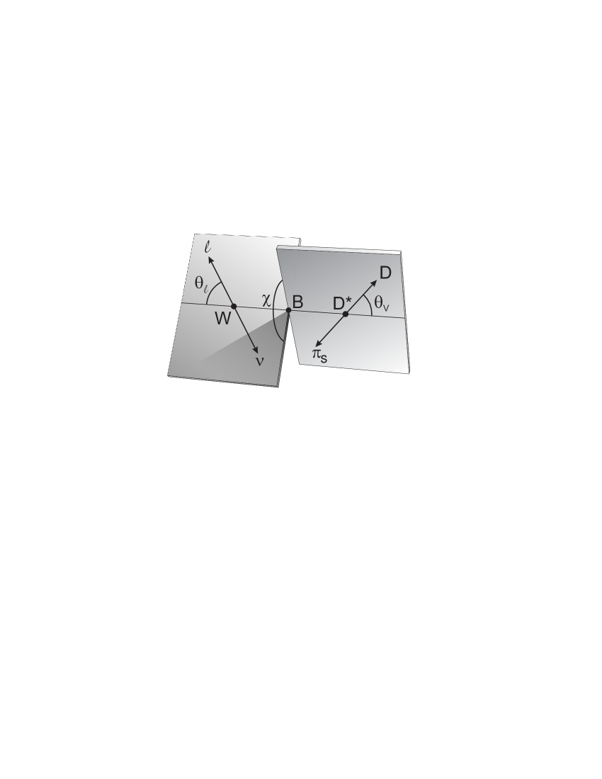
In this analysis we only reconstruct the decay $D^{*+}\mbox{$\rightarrow$}D^{0}\pi^{+}$, where $D^{0}\mbox{$\rightarrow$}K^{-}\pi^{+}$ . The angular variables, shown in Fig. 2, are

Figure 2: Kinematics of a $B\mbox{$\rightarrow$}D^{*}\ell\nu$  decay, mediated by a weak virtual intermediate vector boson $W$. This diagram defines the three kinematic variable angles ${\theta_{\ell}}$, ${\theta_{V}}$ and ${\chi}$.

• ${\theta_{\ell}}$, the angle between the direction of the lepton (i.e., for this analysis, the electron) in the virtual $W$ rest frame, and the direction of the virtual $W$ in the $B$ rest frame

• ${\theta_{V}}$, the angle between the direction of the $D$ in the $D^{*}$ rest frame, and the direction of the $D^{*}$ in the $B$ rest frame

• ${\chi}$, the dihedral angle between the plane formed by the $\mbox{$D^{*}$}-D$ and the plane formed by the $W-\ell$ system.

II.2 Four-Dimensional Decay Distribution

The Lorentz structure of the $B\mbox{$\rightarrow$}D^{*}\ell\nu$ decay amplitude can be expressed in terms of three helicity amplitudes ($\mbox{$H$}_{+}$, $\mbox{$H$}_{-}$, and $\mbox{$H$}_{0}$), which correspond to the three polarization states of the $D^{*}$ (two transverse and one longitudinal). For light leptons these amplitudes are expressed NeubertPhysReport ; richmanburchat in terms of the three form factors:

$$\mbox{$H$}_{+}(w) \equiv -(M_{B}+M_{D^{*}}){A_{1}(w)}+2{\mbox{$\wp_{D^{*}}$}M_{B}\over M_{B}+M_{D^{*}}}{V(w)},$$

$$\mbox{$H$}_{-}(w) \equiv -(M_{B}+M_{D^{*}}){A_{1}(w)}-2{\mbox{$\wp_{D^{*}}$}M_{B}\over M_{B}+M_{D^{*}}}{V(w)},$$

$$\mbox{$H$}_{0}(w) \equiv -{M_{B}+M_{D^{*}}\over M_{D^{*}}\sqrt{q^{2}}}\left[{A_{1}(w)}(M_{D^{*}}(wM_{B}-M_{D^{*}}))\right.$$

$$\hskip 113.81102pt\left.-{4M_{B}^{2}\wp_{D^{*}}^{2}\over(M_{B}+M_{D^{*}})^{2}}{A_{2}(w)})\right],$$

where $\wp_{D^{*}}\equiv M_{D^{*}}\sqrt{w^{2}-1}$ is the magnitude of the momentum of the $D^{*}$ in the $B$ rest frame (for the $\tau$ lepton, which has non-negligible mass compared to the other particles in this process, a fourth helicity amplitude, $H_{t}$, would contribute NeubertPhysReport ).

The full differential decay rate in terms of the three helicity amplitudes is NeubertPhysReport ; richmanburchat

$${d\Gamma\over dq^{2}\;d{\cos\theta_{\ell}}\;d{\cos\theta_{V}}\;d\chi} = {3G^{2}_{F}|V_{cb}|^{2}\mbox{$\wp_{D^{*}}$}q^{2}\over 8(4\pi)^{4}M_{B}^{2}}{\cal B_{\rm D^{*}D}}\times$$

$$\left[{H_{+}^{2}}(1-{\cos\theta_{\ell}})^{2}\sin^{2}\theta_{V}+\right.$$

$${H_{-}^{2}}(1+{\cos\theta_{\ell}})^{2}\sin^{2}\theta_{V}+$$

$$4{H_{0}^{2}}\sin^{2}\theta_{\ell}\cos^{2}\theta_{V}$$

$$-2{H_{+}H_{-}}\sin^{2}\theta_{\ell}\sin^{2}\theta_{V}\cos 2\chi$$

$$-4{H_{+}H_{0}}{\sin\theta_{\ell}}(1-{\cos\theta_{\ell}}){\sin\theta_{V}}{\cos\theta_{V}}\cos\chi$$

$$\left.+4{H_{-}H_{0}}{\sin\theta_{\ell}}(1+{\cos\theta_{\ell}}){\sin\theta_{V}}{\cos\theta_{V}}\cos\chi\right],$$

where ${\cal B_{\rm D^{*}D}}\equiv BF(\mbox{$D^{*+}$}\mbox{$\rightarrow$}\mbox{$D^{0}$}\mbox{$\pi^{+}$})\times BF(\mbox{$D^{0}$}\mbox{$\rightarrow$}K^{-}\mbox{$\pi^{+}$})$ and where all three of the $H_{i}$ are functions of $w$. The four-dimensional distribution of $w$, ${\cos\theta_{\ell}}$, ${\cos\theta_{V}}$, and $\chi$ described by Eq.(II.2) is the physical observable from which we extract the form factors.

In this analysis we only deal with the shape and relative normalization of the form factors, and consequently the overall normalization of the rate is irrelevant.

II.3 Heavy Quark Symmetry Relations

The functions $R_{1}(w)$ and $R_{2}(w)$ are defined in terms of the axial and vector form factors by

$$A_{2}(w)\equiv\frac{R_{2}(w)}{R^{*2}}\frac{2}{w+1}A_{1}(w),$$ (6)

and

$$V(w)\equiv\frac{R_{1}(w)}{R^{*2}}\frac{2}{w+1}A_{1}(w),$$ (7)

where the constant $R^{*}$ is defined by

$$R^{*}\equiv{{2\sqrt{M_{B}M_{D^{*}}}}\over{(M_{B}+M_{D^{*}})}}.$$ (8)

Perfect HQS implies that $R_{1}(w)=R_{2}(w)=1$, i.e., the form factors $A_{2}$ and $V$ are identical for all values of $w$ and differ from $A_{1}$ only by a simple kinematic factor. Since HQS is not exact, in general $R_{1}$ and $R_{2}$ will differ from unity and exhibit some $w$-dependence as discussed in Sec. II.4.

It is conventional to introduce

$$h_{A_{1}}(w)\equiv\frac{1}{R^{*}}\frac{2}{w+1}{A_{1}}(w),$$ (9)

such that in the HQS limit, $h_{A_{1}}$ is the Isgur-Wise function $\xi(w)$ isgurwise and $h_{A_{1}}(1)=\xi(1)=1$.

The function $h_{A_{1}}$ can be parameterized in a number of ways. One simple empirical expansion in $w-1$ is

$$h_{A_{1}}(w) = h_{A_{1}}(1)\times$$

$$\left(1-\rho^{2}(w-1)+\lambda(w-1)^{2}+\kappa(w-1)^{3}+...\right),$$

We will not fit with this general expansion as there are good theoretical constraints (see Eq. (II.3)), which relate all the higher-order parameters to the linear $\rho^{2}$ parameter. Further, convergence issues arise with attempts to fit a free functional form with so many parameters (see Sec. VII.2).

Corrections to HQS modify $h_{A_{1}}(1)$ and thus lead to deviations from the relation of $h_{A_{1}}(1)=1$. In the baseline analysis we use a parameterization of $h_{A_{1}}$ which conforms to requirements of analyticity. This was first developed and presented by Boyd, Grinstein, and Lebed  GrinsteinLebed , though the form used here employs a version of this parameterization proposed by Caprini, Lellouch, and Neubert (CLN) CLN

$$h_{A_{1}}(z) = h_{A_{1}}(1)\times$$

$$\left[1-8{\mbox{$\rho^{2}$}}z+(53{\mbox{$\rho^{2}$}}-15)z^{2}-(231{\mbox{$\rho^{2}$}}-91)z^{3}\right],$$

where

$$z\equiv{{\sqrt{w+1}-\sqrt{2}}\over{\sqrt{w+1}+\sqrt{2}}}.$$ (12)

The maximum value of $z$ over the entire allowed range of $w$ is $z_{max}=0.04$. In an expansion in $z(w)$ to ${\cal O}(w-1)$, $\rho^{2}$ is the coefficient of the linear term. In this case, $\rho^{2}$ can be referred to simply as the slope $\frac{dh_{A_{1}}}{dw}$ at $w=1$. However, in higher-order expansions of $z(w)$, the coefficient of $(w-1)^{2}$, called the “curvature,” will take on non-zero values, as will coefficients of $(w-1)^{3}$ and other higher-order terms. Thus, even though only the single parameter $\rho^{2}$ is used, the functional form of Eq.(II.3) implies a non-linear function for $\mbox{$h_{A_{1}}$}(w)$.

An alternative parameterization motivated by HQS is

$$h_{A_{1}}(w)=\left(\frac{2}{w+1}\right)^{2\rho^{2}}.$$ (13)

Le Yaouanc, Oliver and Raynal have demonstrated that this form obeys the bounds on the derivatives they obtain in the HQS limit using a rigorous, general approach based on Bjorken-like sum rules oliver .

We do not use this form in our analysis, but note that in the $\rho^{2}$ range of interest ($\sim 1-1.5$) it agrees with CLN to a few percent. Thus, $\rho^{2}$ obtained using this parameterization would be virtually identical to that we obtain using Eq.(II.3).

II.4 Form-Factor Ratios

As discussed in Sec. II.3, for infinitely massive $b$ and $c$ quarks, HQS predicts ${\mbox{$R_{1}$}}={\mbox{$R_{2}$}}=1$ exactly. However, these simple relations are broken for finite $b$ and $c$ quark masses, because these ratios are modified by both perturbative ($\alpha_{s}$-dependent) and non-perturbative ${\left({\mathchar 28931\relax_{\rm QCD}\over m_{x}}\right)}$ corrections, where $m_{x}$ represents either the $b$ or $c$ quark mass.

Calculating higher-order loop corrections to the form factors yields expansions of the form LigetiGrinstein :

$${{\mbox{$R_{1}$}}}(w) = 1+\left[\phi_{11}\mbox{$\alpha_{s}$}+\phi_{12}\mbox{$\alpha_{s}^{2}\ $}\right]+\omega_{1}{\left({\mathchar 28931\relax_{\rm QCD}\over m_{x}}\right)},$$ (14)

$${{\mbox{$R_{2}$}}}(w) = 1+\left[\phi_{21}\mbox{$\alpha_{s}$}+\phi_{22}\mbox{$\alpha_{s}^{2}\ $}\right]+\omega_{2}{\left({\mathchar 28931\relax_{\rm QCD}\over m_{x}}\right)}.$$ (15)

The coefficients $\phi_{ij}$ of the $\alpha_{s}$ terms are complicated expressions of the $D^{*}$ boost $w$ which have been calculated perturbatively up to second order, to an estimated accuracy of about one percent (see LigetiGrinstein ). Though they are not explicitly suppressed by a $1\over m_{Q}$  heavy quark mass corrections, they are all functions that approach zero in the $w\mbox{$\rightarrow$}1$ HQS limit.

The coefficients $\omega_{i}$ of the ${\left({\mathchar 28931\relax_{\rm QCD}\over m_{x}}\right)}$ factors are called “subleading Isgur-Wise functions.” Subleading Isgur-Wise function correction terms are evaluated somewhat differently in various models in the HQET framework, resulting in a variety of predictions for ${\mbox{$R_{1}$}}(w)$ and ${\mbox{$R_{2}$}}(w)$.

Perturbative quantum chromodynamics (QCD) and a variety of other theoretical tools have been employed to determine the behavior both at and away from the $w=1$ endpoint. Close and Wambach used a simple quark model CloseWambach to find

$${{\mbox{$R_{1}$}}}(w) = 1.15-0.07(w-1),$$ (16)

$${{\mbox{$R_{2}$}}}(w) = 0.91+0.04(w-1).$$ (17)

Calculations with HQET have produced a variety of results. An early prediction by Neubert was NeubertPhysReport

$${\mbox{$R_{1}$}}(\mbox{${w}$}) = 1.35-0.22(w-1)+0.09(w-1)^{2},$$ (18)

$${\mbox{$R_{2}$}}(\mbox{${w}$}) = 0.79+0.15(w-1)-0.04(w-1)^{2}.$$ (19)

More recently, CLN CLN used spectral functions, dispersion relations, and HQS to predict

$${{\mbox{$R_{1}$}}}(w) = 1.27-0.12(w-1)+0.05(w-1)^{2},$$ (20)

$${{\mbox{$R_{2}$}}}(w) = 0.80+0.11(w-1)-0.06(w-1)^{2}.$$ (21)

Ligeti and Grinstein LigetiGrinstein using similar HQET calculational tools find

$${{\mbox{$R_{1}$}}}(w) = 1.25-0.10(w-1),$$ (22)

$${{\mbox{$R_{2}$}}}(w) = 0.81+0.09(w-1).$$ (23)

It can be seen that in all the predictions the coefficients of the $(w-1)$ and $(w-1)^{2}$ terms are small; this is because $R_{1}$ and $R_{2}$ are, by construction, ratios that are expected to vary only slightly with $w$, whereas $h_{A_{1}}$ is not subject to such a restriction. For the predictions above, $R_{1}$ and $R_{2}$ vary by $0.07$ or less over the full $w$ range. For this reason, for our baseline fit, we follow precedent in treating $R_{1}$ and $R_{2}$ as constants, independent of $w$. We will however examine deviations from this baseline fit in Sec. VII.

III The BABAR Detector

The BABAR detector is described elsewhere in detail ref:babar . This analysis uses four of the five subdetectors of BABAR: the silicon vertex tracker, the drift chamber, a Cerenkov-light-based particle identification detector, and the electromagnetic calorimeter. The analysis depends critically on the silicon vertex tracker to reconstruct the low-momentum pions produced by the decay $D^{*+}\rightarrow D^{0}\pi^{+}$, about two-thirds of which do not traverse more than the first quarter of the drift chamber (as is commonly done, we refer to these as “slow” pions, henceforth denoted “$\pi_{s}$”).

IV Reconstruction and Event Selection

We reconstruct the electron track in the drift chamber and silicon tracker and identify it using particle identification (PID) information from $dE/dx$ measured in the drift chamber, photons captured by the Cherenkov-light detector, and energy deposited in the electromagnetic calorimeter. The $D^{*}$ is reconstructed through its decay to a low momentum pion ($\pi_{s}$) and a $D^{0}$, and the $D^{0}$ through its decay to $K\pi$. The hadrons are selected by similar PID information to that used for the electron identification.

We then choose final cuts that select $B\mbox{$\rightarrow$}D^{*}e\nu$ decay candidates, and from the four-momenta of the observed particles we determine the kinematic variables $w$, ${\cos\theta_{\ell}}$, ${\cos\theta_{V}}$, and $\chi$.

IV.1 Backgrounds and Event Selection

IV.1.1 Background Categories

We address each distinct source of background with appropriate cuts (which are further described below in Sec. IV.1.2):

1. Combinatorial background: events in which the reconstructed $D^{*}$ candidates that were not originally actual ${D^{*}}$ mesons. These events do not contribute to the peak in the $\Delta m=m_{K\pi^{+}\pi^{-}}-m_{K\pi}$ distribution. Cutting on $\Delta m$ provides discrimination against this background.

2. Peaking background, for which the $D^{*}$ decay has been correctly reconstructed and which contributes to the peak in the $\Delta m$ distribution. This category is further broken into two main sub-categories:

   1. $D^{**}$ background: Events where a true $D^{*}$ is combined with a electron from the same $B^{0}$ or $B^{-}$ parent, but an extra pion in the decay has been missed. This is primarily feed-down from P-wave $D$ meson decays, but also includes non-resonant $B\mbox{$\rightarrow$}D^{*}e\nu X$ decays, where $X$ is $n\pi$ ($n\geq 1$). As shorthand we call this “$D^{**}$ background” after its dominant component. Note though that the four P-wave $D$ meson states are usually referred to by the shorthand term “$D^{**}$ modes” in the literature, and thus our redefinition for the purposes of this paper of “$D^{**}$ background” differs slightly from the standard terminology.

   2. Other events with a true $D^{*}$:

      • Fake electron: Events in which a real $D^{*}$ is combined with a hadron instead of an electron. This background is minimized by requiring electrons to pass the most stringent electron-identification criteria.

      • Cascades: Events with a decay chain of the form $\overline{B}^{0}$ or $B^{-}\rightarrow\mbox{ $D^{*}$}X$, $X\rightarrow eY$ (X is e.g., another $D^{*}$ or $D^{0}$, Y is anything), so that the observed electron is not primary (i.e., not directly from a $B$ decay). Secondary electrons have a softer momentum spectrum than primary electrons so that a minimum electron momentum cut is effective against this background source.

      • Uncorrelated electron: Events where a $D^{*}$ is combined with a electron from the other $B$. Thus, one side has a $\overline{B}^{0}$ or $B^{-}\rightarrow D^{*}X$, and the other has $B^{0}$ or $B^{+}\rightarrow Ye$. A cut on $\cos\theta_{BY}$, the cosine of the angle between the $B$ and the $D^{*}-e$ combination, is effective against this background.

      • Continuum: $e^{+}e^{-}\mbox{$\rightarrow$}\ c\overline{c}$ events for which one $c$ quark forms a $D^{*}$ while the other hadronizes into a state which decays semileptonically to create an electron ($c\overline{c}\rightarrow D^{*}eX$). The other continuum backgrounds ($e^{+}e^{-}\mbox{$\rightarrow$}u\overline{u},d\overline{d},s\overline{s}$) are negligible and almost none of them pass the final cuts. Cuts on the $D^{*}$ momentum and event topology are effective at suppressing this background.

IV.1.2 Event Selection Cuts

For event selection we use the procedure developed for the BABAR $V_{cb}$ analysis babarVcb . The most salient cuts are as follows:

• The momentum of the electron in the center-of-mass (C.M.) frame, which is denoted throughout this paper as “$p^{*}_{\ell}$”, is required to be larger than $1.2{\mathrm{\,Ge\kern-1.00006ptV\!/}c}$. This criterion selects $B$ semileptonic decays and suppresses continuum ($\mbox{$e^{+}$}\mbox{$e^{-}$}\mbox{$\rightarrow$}c\bar{c}$) and cascade ($B\mbox{$\rightarrow$}D\mbox{$\rightarrow$}e$) backgrounds.

• The slow pion from the $D^{*}$ decay must have a transverse momentum $p_{t}$ greater than $50{\mathrm{\,Me\kern-1.00006ptV\!/}c}$. This rejects the mostly fake tracks found below this cut. The efficiency for finding true pion tracks below $50{\mathrm{\,Me\kern-1.00006ptV\!/}c}$ is small as the majority of the pions stop before leaving enough hits in the vertex detector to be reconstructed.

• The $\chi^{2}$ probability of the fit of the $D^{*}e$ vertex, including the beam-spot contraint, must be greater than $1\%$. This suppresses inclusion of particles from the other $B$, e.g., those tracks in uncorrelated electron background events.

• To further suppress continuum background, we select only candidates with $|\cos\theta_{\rm thrust}|<0.85$, where $\theta_{\rm thrust}$ is the angle between the thrust axis of the $D^{*}e$ candidate and the thrust axis of the rest of the event.

• The cosine of the angle $\theta_{BY}$ between the direction of the $B$ and the direction of the $D^{*}-\ell$ system can be computed from the kinematics of the ${B^{0}\rightarrow D^{*}\ell\nu}$  decay (see Sec. IV.2). Candidates with $\cos\theta_{BY}$ between $-10$ and $+5$ have been used to estimate background. We include only events that have $|\mbox{$\cos\theta_{BY}$}|\leq 1.2$ in the final sample. The cut is set beyond the physical limits at $\pm 1$ to allow for spillover due to resolution.

• The final selection is based on $\Delta m\equiv m_{K\pi\pi_{s}}-m_{K\pi}$ (the difference between the reconstructed $D^{*}$ and $D^{0}$ masses). We require $0.143\leq\Delta m\leq 0.148$ ${\mathrm{\,Ge\kern-1.00006ptV\!/}c^{2}}$.

Figure 3: Reconstructed particle directions and $\cos\theta_{BY}$ in the CM frame. The momentum vectors $\vec{\bf P}_{D^{*}}$ and $\vec{\bf P}_{\ell}$ are measured. Their sum is $\vec{\bf P}_{Y}$. The magnitude of the $B$ momentum, $\wp_{B}\equiv|\vec{\bf P}_{B}|$, and the angle $\theta_{BY}$ the $B$ makes with $\vec{\bf P}_{Y}$ are known, but the azimuthal orientation $\phi_{BY}$ of $\vec{\bf P}_{B}$ around $\vec{\bf P}_{Y}$ is not known. The points at $\phi_{BY}=0,\pi$ are in the $D^{*}-\ell$ plane.

IV.2 Determination of Kinematic Variable $w$

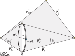
Lacking a measurement of the neutrino momentum, we do not have sufficient information to fully reconstruct the kinematic variables $w$, ${\cos\theta_{\ell}}$, $\cos\theta_{V}$, and $\chi$. However, using energy-momentum conservation and assuming that the missing particle is a massless neutrino, we have

$$0=m^{2}_{\nu}=M_{B}^{2}+M_{Y}^{2}-2E_{B}E_{Y}+2\wp_{B}\wp_{Y}\cos\theta_{BY},$$ (24)

where $p_{Y}\equiv p_{D^{*}}+p_{\ell}$ is the four momentum of the combined $D^{*}$ and electron, $M_{Y}^{2}=p_{Y}^{2}$ is the mass squared and $\wp_{Y}$ is the magnitude of the $Y$ three-momentum. The $B$ meson energy $E_{B}$ and three-momentum magnitude $\wp_{B}$ are known from the energies of the colliding beam particles, so we can solve for $\cos\theta_{BY}$:

$$\cos\theta_{BY}=-\frac{M_{B}^{2}+M_{Y}^{2}-2E_{B}E_{Y}}{2\wp_{B}\wp_{Y}}.$$ (25)

Thus we can determine the angle between the $B$ and the direction ($\hat{Y}=\vec{p}_{Y}/\wp_{Y}$, where $\vec{p}_{Y}$ is the three-vector momentum of the $Y$) of the $D^{*}-\ell$ system, but we do not know the azimuthal angle $\phi_{BY}$. This is illustrated in Fig. 3 where it can be seen that the direction of the $B$ must lie on the cone centered on $\hat{Y}$ with the opening angle $\theta_{BY}$.

For each possible $\phi_{BY}$ we can compute the kinematic variables $w$, ${\cos\theta_{\ell}}$, ${\cos\theta_{V}}$, and $\chi$. Since the angle $\phi_{BY}$ is not measured, we average over four points: two in the $D^{*}$-electron plane corresponding to the azimuthal angles $\phi_{BY}=0$ and $\pi$ and two points out of the plane corresponding to the angles $\pm\pi/2$. Further, since $B\bar{B}$ production follows a $\sin^{2}\theta_{B}$ distribution in the angle between the $B$ direction and the beam collision axis in the CM ($\mathchar 28935\relax(4{\rm S})$) frame, we weight the kinematic variables evaluated at each point by $\sin^{2}\theta_{B}$.

Figure 4: Monte Carlo assessment of the experimental resolution for the variables $w$, ${\cos\theta_{\ell}}$, ${\cos\theta_{V}}$, and $\chi$. For each variable the difference between reconstructed and generated values is shown. The resolutions are small compared to the kinematic ranges of the variables as shown in Fig. 5.

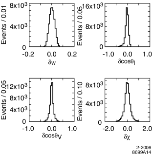
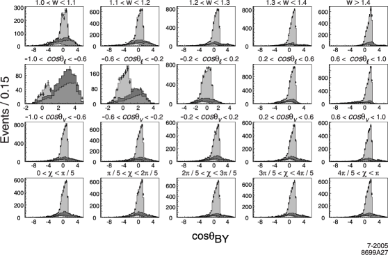
Fig. 4 illustrates the resolution achieved by this technique. The core widths for each resolution distribution are small compared to the full range of each kinematic variable. The resolution is dominated by the average over the $B$ direction; detector resolution makes a relatively minor contribution. The low-side tail on ${\cos\theta_{\ell}}$ can be attributed to final state radiation.

The resolutions of the four kinematic variables are highly correlated. Thus, we rely on Monte Carlo simulation to account for resolution effects.

Figure 5: One-dimensional projections from Monte Carlo simulation of kinematic variables $w$, ${\cos\theta_{\ell}}$, ${\cos\theta_{V}}$, and $\chi$ for selected events. The blank region represents signal, and the shaded regions are estimated backgrounds; the histograms are a sum of both the signal and the estimated background beneath them.

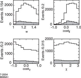
The distributions of the reconstructed kinematic variables $w$, ${\cos\theta_{\ell}}$, ${\cos\theta_{V}}$, and $\chi$ from Monte Carlo simulation are displayed in Fig. 5. The shaded region is the distribution of the background as estimated from the Monte Carlo simulation using the method described in Sec. VI below. The background contributions to the distributions are much smaller than the signal contribution (on the order of 10-15%).

V Simulation

This analysis is dependent on Monte Carlo (MC) simulation to model the efficiency and the background distributions. The degree to which the simulation reproduces both the detector response and the underlying physics processes largely determines the systematic errors.

The response of the BABAR detector is modeled using a GEANT4-based simulation.  babarsim . The simulation has been extensively validated by comparison with large data control samples (such as slow pions from generic $D^{*}\mbox{$\rightarrow$}\mbox{$D^{0}$}\pi$ decays for the slow pion helicity studies). Event generation and particle decay are modeled using the package EvtGen evtgen .

Figure 6: Events vs. the cosine of the slow pion angle relative to the line-of-flight of the $D^{*}$, shown for bins of CM momentum of the $D^{*}$. The momentum ranges for each plot, in GeV/c, are indicated in the upper left-hand corners. Data (points) and MC simulation (histogram) are shown for slow pions from the decay of inclusively produced $D^{*}$ mesons. The vertical scale is arbitrary, but corresponds to the number of background-subtracted reconstructed $D^{*}$ candidates in a given bin. Only the differences between data and MC points are relevant for our purposes. The errors are comparable to the dots representing the data. The simulation has been weighted by restricted functions to fit to the data as described in the text.

V.1 Signal

To simulate the signal we use Eq. (II.2) for the distribution of the decay products. The MC samples are generated with the default parameters $R_{1}=1.180$, $R_{2}=0.720$ and ${\mbox{$\rho^{2}$}}=0.920$ Ryd . The MC generator uses a simple linear expansion (Eq. (II.3) taken to order $(w-1)$), so we must reweight the MC events to model a more complex behavior such as that given by Eq. (II.3).

V.2 Detection of Slow Pions

Of particular importance to this analysis is the modeling of the efficiency for detecting low-momentum pions. This task requires detailed simulation work since low momentum pions are lost through the interplay of acceptance, decay-in-flight, and stopping and scattering in the beam pipe and vertex detector.

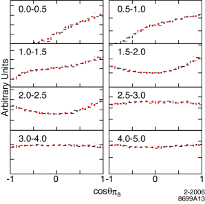
To test this modeling we examine a large control sample of inclusively produced $D^{*+}$ mesons. Fig. 6 shows the distribution of cosine of the helicity angle for the decay $D^{*+}\rightarrow D^{0}\pi^{+}$ reconstructed in both the data and the MC sample in bins of $D^{*+}$ center-of-mass momentum. The helicity is defined so that slower pions correspond to backward helicity angle (and is $\cong-{\cos\theta_{V}}$).

The MC distributions have been fit to the data using a simple weighting factor of the form

$$f_{\rm corr}=N\left(1+\xi_{j}\cos\theta_{\pi_{s}}+\zeta_{j}\cos^{2}\theta_{\pi_{s}}\right),$$ (26)

where the normalization $N$ and the parameters $\xi_{j}$ and $\zeta_{j}$ have been obtained for each momentum bin ${j}$. The three lowest momentum bins are most relevant to $B\mbox{$\rightarrow$}D^{*}\ell\nu$ decays. The agreement between the weighted simulation and the data is excellent. Note the weighting factor Eq.(26) is not applied to correct the signal. Rather the weight coefficients obtained by fitting this control sample measure the MC-data differences in each momentum bin.

The linear terms, $\xi_{j}$, arise from inadequacies in the simulation of the detector response. The linear terms for the first three bins are small: $0.037\pm 0.160$, $-0.023\pm 0.024$ and $-0.016\pm 0.009$, indicating good agreement between the data and Monte Carlo simulation efficiencies in the complicated arena of slow pion modeling. Note that critical details of the distributions that are unaffected by the weighting scheme (such as the evident thresholds in the low momentum bins) are reproduced correctly by the MC.

The quadratic terms arise mostly from incorrect simulation of the polarization of the $D^{*}$-mesons. The values of $\zeta$ are large ($\sim 0.5$ and $0.7$) in the momentum bins for $0.5-1.0$ GeV/$c$ and $1.0-1.5$ GeV/$c$, where we expect $D^{*}$-mesons to be highly polarized products of few-body $B$-meson decays. These terms do not indicate any problem with detector simulation, and only affect a tiny fraction of the events in our final sample (the fake electron background).

Further, as the MC and data agree well for the linear terms, there is no need to make corrections to account for differences between simulation and data. This is further indicated by the lower right plot of $p_{t,\mbox{$\pi_{s}$}}$ shown in Fig. 12, which indicates excellent agreement between the slow pion transverse momentum distribution after the final fit, but with no linear weighting terms applied to the slow pion momentum.

As the extraction of form factors (especially $\rho^{2}$) is highly sensitive to the slow pion simulation we do add a contribution to the systematic error to account for the possible residual differences between the data and the MC simulation. We describe our method for doing this in Sec. IX.1.3.

V.3 Final State Radiation

The program PHOTOS Was is used to model the effects of final state radiation (FSR). PHOTOS uses quantum electrodynamics (QED) to second order in $\alpha_{em}$ (up to two FSR photons can be produced) and is known to provide a quite accurate simulation of the FSR effects WasII .

V.4 Other Semileptonic Decays

A major source of background is other semileptonic $B$ decays. Only the branching fractions for the decay modes $D\ell\nu$, the signal mode $D^{*}\ell\nu$, and that for the mode $B\mbox{$\rightarrow$}D_{1}\ell\nu$ have been measured pdg2004 (i.e., only one of the four P-wave $D$ meson states). The other branching fractions (including the three other P-wave $D$ states and all non-resonant decays) used in the MC simulation are based on models with large theoretical uncertainties. We use fits to the data to constrain these branching fractions as shown in Sec. IX, to minimize their contribution to the systematic background error.

VI Analysis Method

VI.1 Fitting

Our approach to extracting the form factors is to perform an unbinned maximum likelihood fit to the full four-dimensional distribution function (PDF) specified by Eq. (II.2). We parameterize the form factors in terms of the parameters $R_{1}$, $R_{2}$ and $\rho^{2}$ as described in Sec. II. The $\rho^{2}$ dependence is specified by Eq. (II.3). Since theoretical predictions show only a mild dependence of $R_{1}$ and $R_{2}$ on $w$ (see Eqs. (16-18), we first perform the fit treating them as constants over the entire range of $w$. We later show (in Sec. VII) how the results vary when the $w$-dependencies suggested by the Eqs. (16-18 are imposed.

In addition to assuming its form, we must account for the effects of resolution and efficiency on the measured distribution. We adopt approximations that enable us to carry out the maximum likelihood fit to the form factor parameters efficiently with minimal loss in precision.

VI.1.1 Resolution-Efficiency Correction Method

To account for the efficiency and resolution effects we adapt the approach first employed in the angular analysis of the decay $B\rightarrow J/\psi K^{*}$psikstar (for more details of the technique see also Gill ). The full PDF (${\cal F}$) including resolution and efficiency is given in terms of the theoretical PDF ($F$) of Eq. (II.2) by

$${\cal F}(\tilde{x};\mu)=\int{dx\,\varepsilon(x)\,G(\tilde{x};x)\,F(x;\mu)},$$ (27)

where $x$ represents the true variables ($w$, ${\cos\theta_{\ell}}$, ${\cos\theta_{V}}$, and $\chi$), $\tilde{x}$ are the observed values of the variables and $\mu$ represents the parameters ($R_{1}$, $R_{2}$ and $\rho^{2}$) that determine the form factors. The efficiency $\varepsilon(x)$ is the fraction of events with parameters $x$ that are detected and $G(\tilde{x};x)$ is the probability density that an event with true parameters $x$ is reconstructed with parameters $\tilde{x}$.

The logarithm of the likelihood $L$ that we need to maximize is given by

$$\ln L=\sum_{i}{\ln\left(\frac{{\cal F}(\tilde{x}_{i};\mu)}{{\cal{I}}(\mu)}\right)}$$ (28)

$$=\sum_{i}{\ln{\cal F}(\tilde{x}_{i};\mu)}-N_{\rm{data}}\times\ln{\cal{I}}(\mu),$$

where the integral

$${\cal{I}}(\mu)\equiv\int{d\tilde{x}{\cal F}(\tilde{x};\mu)}$$ (29)

is required to normalize the likelihood in the presence of imperfect acceptance. The sum is over our data sample of $N_{\rm{data}}$ events.

While the distribution ${\cal F}(\tilde{x},\mu)$ can be simulated by Monte Carlo, it is not practical to use it directly as the function to be varied in the maximum likelihood analysis. Instead, we will introduce a method in which we can use Monte Carlo simulation data without any need to extract a detailed model of the efficiency and resolution function.

We now try the approximation

$${\cal F}(\tilde{x};\mu)\cong f(\tilde{x};\mu)\equiv{\cal F}(\tilde{x};\mu_{\rm mc})\frac{F(\tilde{x};\mu)}{F(\tilde{x};\mu_{\rm mc})}.$$ (30)

where $\mu_{\rm mc}$ is the parameter set used for generation of the Monte Carlo sample. If we had used the true values of the parameters $\mu_{\rm t}$ in place of $\mu_{\rm mc}$, then the maximum likelihood method would converge to the true values since by inspection the trial function $f(\tilde{x};\mu)$ would become the true distribution ${\cal F}(\tilde{x};\mu)$. Of course the true values are not known. The use of $\mu_{\rm mc}$ introduces a bias proportional to the difference between the Monte Carlo parameter values and the true parameter values, which can be calculated explicitly in the limit of high statistics.

When the approximation $f(\tilde{x};\mu)$ of Eq. (30) is substituted into the expression for the log-likelihood Eq. (28), it yields

$$\ln L = \sum_{i}\ln F(\tilde{x}_{i};\mu)-\sum_{i}\ln F(\tilde{x}_{i};\mu_{\rm mc})$$

$$+\sum_{i}\ln{\cal F}(\tilde{x}_{i};\mu_{\rm mc})-N_{\rm{data}}\ln\hat{\cal{I}}(\mu,\mu_{\rm mc}),$$

where $\hat{\cal{I}}(\mu,\mu_{\rm mc})$ is the integral of the approximation of Eq.(30).

Since terms that are independent of the fit parameters (constant terms) do not affect the point at which the maximum will be found, all the sums that depend only on $\mu_{\rm mc}$ can be dropped (i.e., the central two terms of the total sum). The $\mu$-dependent piece has been factored from these constant terms. We are left with a likelihood function that depends only on the theoretical PDF $F$ and on the integral over the resolution and efficiency functions.

The resolution and efficiency occur only through the normalization integral $\hat{\cal{I}}(\mu,\mu_{\rm mc})$.

Using the technique of Monte Carlo integration to evaluate the integral $\hat{\cal{I}}(\mu,\mu_{mc})$ gives

$$\hat{\cal{I}}(\mu,\mu_{\rm mc})=\int{d\tilde{x}{\cal F}(\tilde{x};\mu_{\rm mc})\times\frac{F(\tilde{x};\mu)}{F(\tilde{x};\mu_{\rm mc})}}$$ (32)

$$\approx\frac{1}{N_{\rm gen}}\sum_{i}{\frac{F(\tilde{x}_{i};\mu)}{F(\tilde{x}_{i};\mu_{\rm mc})}}.$$

The MC simulation generates events in proportion to ${\cal F}(\tilde{x};\mu_{\rm mc})$ so the sum over Monte Carlo events approximates the desired integral. The small error introduced by the Monte Carlo evaluation of the normalization integral is determined in Appendix A.

In Appendix A, we demonstrate that the bias introduced by the use of the approximate form Eq.(30) is given by

$$(\mu-\mu_{\rm t})_{a}=\sum_{b}(\mu_{\rm mc}-\mu_{\rm t})_{b}M_{ba}$$ (33)

where

$$M_{ba}=J_{bc}E_{ca},$$ (34)

and

$$J_{bc} \equiv {\left<{\frac{\partial\ln\frac{\cal F}{F}}{\partial\mu_{b}}\frac{\partial\ln F}{\partial\mu_{c}}}\right>-\left<{\frac{\partial\ln\frac{\cal F}{F}}{\partial\mu_{b}}}\right>\left<{\frac{\partial\ln F}{\partial\mu_{c}}}\right>}$$

$$E^{-1}_{ac} \equiv {\left<{\frac{\partial\ln F}{\partial\mu_{a}}{\frac{\partial\ln F}{\partial\mu_{c}}}}\right>-\left<{\frac{\partial\ln F}{\partial\mu_{a}}}\right>\left<{\frac{\partial\ln F}{\partial\mu_{c}}}\right>}$$ (35)

and where averages are defined by

$${\langle A\rangle}\equiv\frac{\int dx{\cal F}(x,\mu_{\rm t})A(x)}{\int dx{\cal F}(x,\mu_{\rm t})}.$$ (36)

The bias vanishes if the parameters used in the Monte Carlo coincide with the true values. Moreover, the bias vanishes insofar as the ratio ${\cal F}/F$ of the smeared distribution to the unsmeared distribution is independent of the parameters $\mu$. Since ${\cal F}$ and $F$ probe nearby regions, the derivative of their ratio will be small, so the coefficient $\alpha$ in Eq. (34) should be much less than one. Numerical evaluation yields values of $\sim 0.15$ for $R_{1}$ and $R_{2}$ and $\sim 0.03$ for $\rho^{2}$. If $\mu_{\rm mc}-\mu_{\rm t}$ is comparable to the error, the residual “bias” should be small, and in practice is found to be so.

To achieve $\mu_{\rm mc}\sim\mu_{\rm t}$ we reweight the MC used in the efficiency integral computation to the fitted values of the parameters and iterate until the fit values converge. At this point $\mu_{\rm mc}=\mu_{fitted}$ and should deviate from the truth by an amount comparable to the error. In effect the residual deviation acts like a small increase ($\sim 2\%$) in the statistical uncertainty. The iteration method works well and converges quickly, as discussed further in Sec. VII.3.

VI.1.2 Speeding Computation of Normalization Integral Through Moments Factorization

Because the normalization integral $\hat{\cal{I}}(\mu,\mu_{\rm mc})$ depends explicitly on $\mu$ it must be recomputed for every iteration of the procedure that maximizes the log-likelihood. To do this by Monte Carlo integration over the full decay phase space would be prohibitively slow.

For the signal distribution, this integration can be avoided. Since the signal PDF can be written in the following form,

$$F(\tilde{x};\mu)=\sum_{\alpha}{A_{\alpha}(\mu)\times\mathchar 28932\relax_{\alpha}(x)},$$ (37)

i.e., as sum over a product of terms depending only on the fit parameters and terms depending only on the kinematic variables, we can define moments $M_{\alpha}$ by

$$M_{\alpha}=\frac{1}{N_{gen}}\sum_{i}{\frac{\mathchar 28932\relax_{\alpha}(\tilde{x}_{i})}{F(\tilde{x}_{;}\mu_{\rm mc})}},$$ (38)

where the sum is over reconstructed MC events, i.e., the same sum that defines $\hat{\cal{I}}(\mu,\mu_{\rm mc})$ in Eq. (32). This allows us to write $\hat{\cal{I}}(\mu,\mu_{\rm mc})$ as a sum over moments:

$${\hat{\cal{I}}(\mu,\mu_{\rm mc})}=\sum_{\alpha}{A_{\alpha}(\mu)\times M_{\alpha}}.$$ (39)

The moments can be computed once before fitting and then taken as input to the fit. Thus, in the fit, the time-consuming sum over weighted events is replaced with the sum over moments. Taking the expansion of $h_{A_{1}}$ to order $(w-1)^{3}$ or $z^{3}$, we have 42 moments to compute and sum.

VI.1.3 Background Subtraction Through Pseudo-Likelihood

To handle the background, we would ordinarily add a PDF $B(\tilde{x})$ that models the background. The PDF ${\cal F}$ would be replaced with

$$f{\cal F}(\tilde{x};\mu)+(1-f)B(\tilde{x}),$$ (40)

where $f$ is the signal fraction. However, since we do not have a form for the background distribution before acceptance, we cannot achieve the factorization of the parameter dependence from the efficiency and resolution functions that leads to Eq. (39). To avoid this problem we use the technique of subtracting Monte Carlo events representing the background directly in our likelihood sum rather than adding it to our PDF. We replace our log-likelihood function with the following ‘pseudo-likelihood’ BbrPseudoL

$$\ln\mathchar 28931\relax = \sum_{i\in{\rm data}}\ln F(x^{(i)}_{\rm data};\mu)-$$

$$\sum_{j\in{\rm MC}}W^{(j)}_{\rm bkgd}\ln F(x^{(j)}_{\rm bkgd};\mu)-N_{{\rm signal}}\ln{\cal{I}}(\mu),$$

where the first sum is over the data and the second is over a Monte Carlo sample representative of the background. The weights $W^{(i)}_{\rm bkgd}$ account for any difference between the background in the data and in the Monte Carlo. They are computed in the manner indicated by Eqs. (42) and (44) in Sec. VI.3 below. The coefficient of the normalization integral is $N_{\rm signal}=N_{\rm data}-N_{\rm bkgd}$, where $N_{\rm bkgd}$ is equal to the number of events subtracted, accounting for the weights. It is easy to show that if the Monte Carlo simulation of the background is accurate, the procedure is unbiased. The statistical errors can be computed by a modification of the procedure used for an ordinary log-likelihood analysis.

VI.2 Methodological Error Contributions

The approximations outlined above provide a fast and easily-implemented fitting procedure that uses the MC sample without any need to extract a detailed model of the efficiency and resolution functions. However, these advantages do not come without a cost: we must account for the uncertainty introduced by the resolution-efficiency and pseudo-log-likelihood procedures.

There are three other contributions to the error that are not accounted for in the fit. Two of these are Monte Carlo statistical in nature: the error from the pseudo-log-likelihood subtraction and the error from the Monte Carlo integration used to evaluate $\hat{\cal{I}}(\mu,\mu_{\rm mc})$ in the resolution-efficiency correction procedure. There is also a contribution to the statistical error from the fluctuations in the background that are not accounted for in the fit. The first two can be reduced by increasing the size of the Monte Carlo sample, but the latter error is irreducible and must be included regardless of the size of the Monte Carlo sample.

We have developed procedures for evaluating these three errors. The formulas used are collected in Appendix A.

VI.3 Background Level Estimation

The categorization of backgrounds has been detailed in Sec. IV.1. The combinatorial and peaking backgrounds are estimated by fitting the measured $\Delta m=m_{K\pi^{+}\pi^{-}}-m_{K\pi}$ and $\cos\theta_{BY}$ distributions in data. The $\Delta m$ fit determines the combinatorial background. The $\cos\theta_{BY}$ distribution is then fit to a combination of signal, combinatorial background, “$D^{**}$” peaking and other peaking background using the binned likelihood fitting method of Barlow and Beeston bandb . The shape of the $\cos\theta_{BY}$-distributions are taken from the Monte Carlo simulation. In the fit, only the signal fraction and the portion of the peaking background due to ${D^{**}}$ and $D^{*}Xe\nu$ decays are free parameters. The combinatorial fraction is set to the value obtained from the $\Delta m$ fit and the other components of the peaking background are scaled from the Monte Carlo. See Sec. IV.1.1 for more details.

We apply the above procedure first to obtain the overall fractions for the combinatorial ($f_{\rm comb}$) and the ${D^{**}}$ ($f_{D^{**}}$) backgrounds. These are obtained by fitting to the full data sample. The fraction of the consolidated remaining peaking backgrounds ($f_{\rm otherPk}$), detailed in Sec. IV.1.1, is obtained by direct scaling from the MC simulation.

The weight needed to subtract the correct amount of each background type is given by

$$W_{\rm type}=\frac{f_{\rm type}\times{N_{\rm data}}}{N_{\rm type}},$$ (42)

where type=$comb$, ${D^{**}}$ or $other$ depending on the particular background type being subtracted and $N_{\rm type}$ is the number of Monte Carlo events of that type available.

The determination of $f_{\rm comb}$ and $f_{{D^{**}}}$ is discussed in more detail in the next two subsections.

VI.3.1 Determination of Level of Combinatorial Background

The combinatorial background is due to ${D^{*}}$ candidates that were not originally actual ${D^{*}}$ mesons. It includes candidates where the $D$ is properly reconstructed, but is paired with a random $\pi$; events in which the $\pi_{s}$ is in fact from the decay ${D^{*}}\rightarrow D\mbox{$\pi_{s}$}$, but the $D$ is not properly reconstructed; and candidates which are purely combinatoric (neither the $D$ nor the $\pi_{s}$ are correctly reconstructed) – i.e., where any one or more of the three detected particles does not originate from the decay chain $\mbox{ $D^{*}$}\mbox{$\rightarrow$}D\mbox{$\pi_{s}$}\mbox{$\rightarrow$}(K\pi)\mbox{$\pi_{s}$}$.

To model this background we use the following functional form

$${f(\Delta m)=N\left(1-\exp{\left(\frac{\Delta m-\Delta m_{\rm thr}}{s}\right)^{\kappa}}\right)\left(\frac{\Delta m}{\Delta m_{\rm thr}}\right)^{\gamma}},$$ (43)

where below the $D^{*}$ threshold $\Delta m_{\rm thr}$ we take $f(\Delta m)$=0. This is an extension of the commonly used threshold function babarVcb . To the single scale parameter $s$ the power $\kappa$ and the factor $\left({\Delta m}\over{\Delta m_{\rm thr}}\right)^{\gamma}$ have been added as extra degrees of freedom. This extension allows us to obtain a better fit to the background and allows the fit enough freedom to account for the uncertainty in the background shape. Fixing $\kappa=1$ and $\gamma=0$ corresponds to the usual unextended threshold function (further details of the necessity of this extension are given in Appendix B).

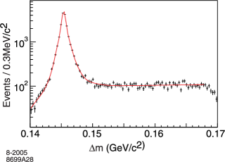
The signal distribution is fit by three free Gaussian functions plus a fixed tail of two wide Gaussians. The tail is fixed by fitting pure signal Monte Carlo as described in Appendix B.

The final fit to data is shown in Fig. 7.

Figure 7: The fit (solid line) to the $\Delta m$ distribution for ${D^{*}}e\nu$ candidates as described in the text. The distribution is shown logarithmically to emphasize details of the functional fit, but the actual level of background is more clearly seen in the linear data plot shown in Fig. 16.

VI.3.2 Determination of Level of $D^{**}$ Background

To estimate the peaking background we use a mixture of Monte Carlo predictions and a fit to the ${\cos\theta_{BY}}$ distribution within the $D^{*}$ signal window $\mbox{$\Delta m$}=0.143--0.148{\mathrm{\,Ge\kern-1.00006ptV\!/}c^{2}}$. We fit the ${\cos\theta_{BY}}$  distribution for the signal and the background due to decays of the type $B\rightarrow D^{*+}Xe\nu$ (called the “$D^{**}$” background, as defined in Sec. IV.1.1). The shapes of the ${\cos\theta_{BY}}$ distributions for the signal and the backgrounds are obtained from the Monte Carlo simulation. The backgrounds other than the $D^{**}$ are fixed at values obtained by scaling from the Monte Carlo by the appropriate luminosity ratios. In the case of fake electrons (which are mostly misidentified pions), we also scale using the misidentification probabilities obtained from the data control sample of pions (specifically from the BABAR $\tau^{\pm}\rightarrow\pi^{\pm}\mbox{$\pi^{+}$}\mbox{$\pi^{-}$}\nu_{\tau}$ dataset).

Figure 8 shows the results of this fit to the full data sample. The shading indicates the background source or signal. Only two paramaters, the signal and the $D^{**}$ background fractions, are free in the fit. The combinatorial background is input from the $\Delta m$ fit. The other peaking backgrounds are scaled from the Monte Carlo simulation as described above.

Figure 8: The ${\cos\theta_{BY}}$ data distribution and the result of the fit with the estimated signal and background contributions, as described in the text. Shading indicates the various components in the fit.

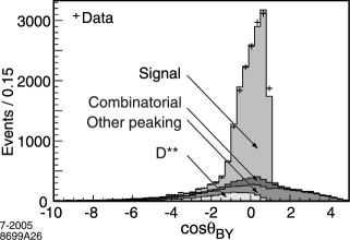
For input to the form-factor fit we need the background fractions within the ${\cos\theta_{BY}}$ signal window ($|{\cos\theta_{BY}}|\leq 1.2$). These are $f_{\rm comb}=5.33\pm 0.26\%$ for the combinatorial, $f_{D^{**}}=4.85\pm 0.35\%$ for the $D^{**}$ and $f_{\rm otherPk}=7.03\pm 0.45\%$ for peaking backgrounds other than the $D^{**}$.

VI.3.3 Dependence of Background Levels on Kinematic Variables

In addition to obtaining overall background fractions, we perform our $\Delta m$-$\cos\theta_{BY}$ fitting procedure in five bins for each of the kinematic variables in the data. This allows extraction of the dependence of combinatorial and ${D^{**}}$ backgrounds for each kinematic variable. We compare the ratio of fitted background yields in data and MC, and parameterize the difference as a linear function of the kinematic variables. This allows application of a correction term to the weight for each Monte Carlo event of the form:

$$W_{\rm type}^{corr}=(1+\alpha_{w}(w-\left<{w}\right>_{\rm type}))$$ (44)

$$\times(1+\alpha_{\cos\theta_{\ell}}({\cos\theta_{\ell}}-\left<{{\cos\theta_{\ell}}}\right>_{\rm type}))$$

$$\times(1+\alpha_{\cos\theta_{V}}({\cos\theta_{V}}-\left<{{\cos\theta_{V}}}\right>_{\rm type}))$$

$$\times(1+\alpha_{\chi}(\chi-\left<{\chi}\right>_{\rm type})),$$

where the means for each type (which are calculated from the Monte Carlo simulation distributions) are subtracted to keep the normalization independent of the slope.

To extract the dependence of combinatorial background on the kinematic variables, the procedure of fitting four Gaussians for the signal (discussed in Appendix B) and the extended threshold function for the combinatorial background portion is repeated for five bins in each of the four kinematic variables.

To obtain the slopes needed in Eq. (44) we form the ratio of the background estimate in each bin to the number found in that bin in the Monte Carlo simulation and fit it to a straight line. All of the fits are displayed in in Fig. 19 Appendix B.

This information is summarized and shown in Fig. 9, and the numerical results for the slopes are given in Table 1 along with the means, which are needed to do normalization independent weighting, as discussed above after Eq. (44).

Figure 9: Ratio of data to Monte Carlo events for combinatorial background for the four kinematic variables $w$, ${\cos\theta_{\ell}}$, ${\cos\theta_{V}}$, and $\chi$, obtained from 5-bin fits to data and Monte Carlo in each kinematic variable. The lines are result of linear fits (see text).

Table 1: The fitted slopes to the distributions shown in Fig. 9 of the ratio of data to Monte Carlo for the combinatorial background in the four kinematic variables $w$, ${\cos\theta_{\ell}}$, ${\cos\theta_{V}}$ and $\chi$, and the mean values of the Monte Carlo distributions for these variables.

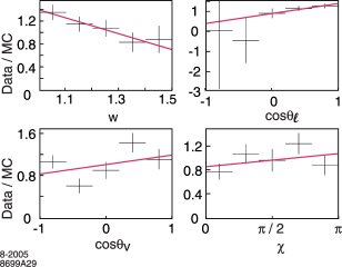
Variable	Slope	Mean
$w$	$\hphantom{+}0.51\pm 0.50$	1.23
${\cos\theta_{\ell}}$	$\hphantom{+}0.05\pm 0.11$	0.31
${\cos\theta_{V}}$	$-0.20\pm 0.09$	0.00
$\chi$	$-0.13\pm 0.06$	1.48

As in the combinatorial case, we repeat the extraction of the ${D^{**}}$ component of the peaking backgrounds in five bins in each of the four kinematic variables. The results of all these ${\cos\theta_{BY}}$ fits are shown in Fig. 20 in Appendix B. This is summarized in the linear fit for data to Monte Carlo events ratio for the $D^{**}$ background (the component free in the fit), which is shown in Fig. 10, with the numerical results in Table 2.

The linear fits in Fig. 10 give the slopes used in weighting the backgrounds using Eq. (44).

We use the central slope values to reweight our background subtraction and propagate the errors into the systematic uncertainty by varying the slopes within their errors.

Figure 10: Ratio of data to Monte Carlo events for $D^{**}$ background for the four kinematic variables $w$, ${\cos\theta_{\ell}}$, ${\cos\theta_{V}}$, and $\chi$, obtained from 5-bin fits to data and Monte Carlo in each kinematic variable. The lines are result of linear fits (see text)

Table 2: The fitted slopes to the $D^{**}$ distributions shown in Fig. 10 of the ratio of data to Monte Carlo for the combinatorial background in the four kinematic variables $w$, ${\cos\theta_{\ell}}$, ${\cos\theta_{V}}$ and $\chi$, and the mean values of the Monte Carlo distributions for these variables.

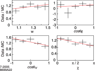
Variable	Slope	Mean
$w$	$-1.35\pm 0.52$	$\hphantom{+}1.28$
${\cos\theta_{\ell}}$	$\hphantom{+}0.14\pm 0.29$	$\hphantom{+}0.35$
${\cos\theta_{V}}$	$\hphantom{+}0.18\pm 0.12$	$-0.11$
$\chi$	+$0.07\pm 0.08$	$\hphantom{+}1.53$

Further details of the fits and estimates for the background fractions and weights are given in Appendix B.

VI.4 $\chi$ Averaging

Few data events arising from true signal will be found at values of the kinematic variables for which the PDF goes to zero. However, there is no such limitation on the number of data events arising from backgrounds that may fall at these points. Because of this, when the logarithm of the PDF is evaluated for these points as part of the background-subtracted computation of the log-likelihood  it develops spuriously large (negative) values, driving the fit far astray from the actual minima.

To deal with these spurious zeros we deliberately introduce a small amount of artificial resolution that prevents the PDF from going to zero. This resolution is chosen to be small compared to the natural resolution of our kinematic variable reconstruction (see Fig. 4) and so has little effect on the sensitivity of our measurement. Any small bias introduced is removed by the resolution-efficiency correction method in the same manner as that due to naturally occurring resolution.

We implement this artificial resolution by evaluating the PDF for all data points (including the data, Monte Carlo-selected background, and integration samples, for consistency) at values of the phase space not exactly at the given point, but offset from it on both sides in $\chi$ by $\pm 0.1$. The kinematic variable $\chi$ is chosen because it is at particular discrete, parameter-dependent values of $\chi$ that the theoretical PDF is zero. We then take the values of the PDF for these two offset points and average them. This average is used as the value for the given point in evaluating its contribution to the likelihood.

Testing on Monte Carlo simulation shows $\chi$-averaging does not bias the fit values, nor increase the errors. Varying the value by which we move $\chi$ we find that $\pm 0.1$ is small enough to not bias the fit values, and large enough to eliminate the spurious zero problems fully, so we evaluate all fit results with this offset.

VII Results

VII.1 Free Parameter and Baseline Fits

We perform the baseline fit (see Sec. II.3) taking $R_{1}$ and $R_{2}$ to be independent of $w$ and use the single parameter form factor description of Ref. CLN given in Eq. (II.3).

We find

$${\mbox{$R_{1}$}}=1.396\pm 0.060\pm 0.035,$$

$${\mbox{$R_{2}$}}=0.885\pm 0.040\pm 0.022,$$ (45)

$${\mbox{$\rho^{2}$}}=1.145\pm 0.059\pm 0.030,$$

where the first uncertainties given are due to the limitations of the data statistics and the second to limitations of statistics of the Monte Carlo simulations. Systematic uncertainties are discussed in Sec. IX below. The errors are highly correlated. The error matrix for the full statistical error for $R_{1}$, $R_{2}$, and $\rho^{2}$ (including Monte Carlo statistical) is:

       0.00479  -0.00243   0.00277
      -0.00243   0.00207  -0.00231
       0.00277  -0.00231   0.00447
       

The correlations are

$$\eta_{R_{1}-R_{2}}=-0.77,$$

$$\eta_{R_{1}-\rho^{2}}=+0.60,$$ (46)

$$\eta_{R_{2}-\rho^{2}}=-0.76.$$

As we do not yet have enough statistical sensitivity to fit for the $w$-dependence of $R_{1}(w)$ and $R_{2}(w)$, we consider instead the effect of the theoretically predicted dependence on the result. Parameterizing this dependence as follows

$$R_{1}(w)=R_{1}+\alpha_{1}(w-1)+\beta_{1}(w-1)^{2},$$ (47)

$$R_{2}(w)=R_{2}+\alpha_{2}(w-1)+\beta_{2}(w-1)^{2},$$ (48)

and inserting these $w$-dependent forms into the PDF (with fixed $\alpha_{i},\beta_{i}$ from the theoretical predictions) and fitting for the constant terms $R_{1}$ and $R_{2}$  we find the results given in Table 3.

Reference	$\alpha_{1}$	$\beta_{1}$	$\alpha_{2}$	$\beta_{2}$	$R_{1}$	$R_{2}$	$\rho^{2}$
Baseline	$\hphantom{+}0.0$	0.0	0.0	$\hphantom{+}0.0$	1.40	0.89	1.15
Caprini-Lellouch-NeubertCLN	$-0.12$	0.05	0.11	$-0.06$	1.42	0.87	1.12
Ligeti-GrinsteinLigetiGrinstein	$-0.10$	0.0	0.09	$\hphantom{+}0.0$	1.42	0.87	1.11
NeubertNeubertPhysReport	$-0.22$	0.09	0.15	$-0.04$	$1.45$	0.86	1.09

Table 3: Dependence of form-factor parameters on theoretical assumptions about slope ($\alpha$) and curvature ($\beta$) of $R_{1}$ and $R_{2}$ $w$-dependence. See Eqs. (47) and (48).

These theoretical variations in $R_{1}(w)$ and $R_{2}(w)$ yield slightly larger values for $R_{1}$ and slightly smaller values for $R_{2}$. However, this is presumably only because they all decrease the mean of $R_{1}(w)$ and increase the mean of $R_{2}(w)$ when averaged over the $w$ spectrum.

VII.2 Higher-Order Free Parameter Fits

We performed a study using a large MC sample in order to ascertain whether it was also useful for us to do free fits to $h_{A_{1}}$ with up to five parameters (see Eq. (II.3)) for a sample generated with a particular form (the CLN form). To this end, we created a MC sample of a million events generated with the ansatz of Eq. (II.3) with no acceptance cuts or resolution smearing applied. We then attempted to fit this using four parameters ( $R_{1}$,$R_{2}$, and coefficients to $\cal O$ $(w-1)^{2}$ in $h_{A_{1}}$) and five parameters ( $R_{1}$,$R_{2}$, and coefficients to $\cal O$ $(w-1)^{3}$ in $h_{A_{1}}$). The fit results for the slope and curvature (for the four parameter fit) and slope, curvature, and cubic term coefficient (for the five parameter fit) were far from the generated values corresponding to the $(w-1)^{n}$ expansion of the input (Eq. II.3).

This problem arises because the fit is attempting to compensate for the missing higher-order terms. As a result the coefficients of $(w-1)$ or $(w-1)^{2}$ returned by the fit cannot be cleanly interpreted in terms of the theoretical expectations or interpreted in terms of limits such as those given in oliver ; oliver2 .

Thus, while either the CLN or free polynomial expansion are a priori valid, the former is preferred from theoretical constraints, and we see from the above that it is not useful to attempt to fit a sample with a free expansion to a reasonably low expansion order and then interpret the result in terms of CLN coefficients.

VII.3 Iterative Convergence Studies

We have studied the convergence of the likelihood maximization procedure described in Sec. VI.A. Varying the initial seed values by as much as 50% of the final values still leads to convergence to the same final values within 0.0005 for each parameter within five iterations.

VIII Goodness-of-Fit

To assess whether the results of the fit reproduce the distribution of the kinematic variables in the data, we use a binned $\chi^{2}$ method of estimating goodness-of-fit. Chernoff and Lehmann chernoff have shown that while a binned $\chi^{2}$ will in general have a wider than expected distribution when the free parameters are optimized using a likelihood fit, the effect is small for a large number of bins. Therefore we adopt the binned $\chi^{2}$ as our primary goodness-of-fit test.

Since we do not have an explicit form for the acceptance-corrected PDF (${\cal F}$) of the four reconstructed variables $w$, ${\cos\theta_{\ell}}$, ${\cos\theta_{V}}$ and $\chi$, we reweight the MC sample to construct the distributions expected from our measured parameters. That is, the contribution of the signal to a bin is given by the MC event sum

$$n_{\rm signal}=\sum_{i\in{\rm MC}}{W^{(i)}_{\rm signal}},$$ (49)

where

$$W^{(i)}_{\rm signal}=f_{signal}\times N_{\rm data}\times\frac{W_{i}}{\sum W_{i}}$$ (50)

and in this case $W_{i}=\frac{F(x_{i};\mu)}{F(x_{i};\mu_{mc})}$ is the weight needed to modify the distributions from those generated with $\mu_{mc}$ ($R_{1}=1.18$, $R_{2}=0.72$, and $\rho^{2}=0.92$), to those obtained from this analysis and $f_{\rm signal}=1-f_{D^{**}}-f_{\rm otherPk}-f_{\rm comb}$ is the signal fraction.

For the background we use the same weighting procedure (see Eqs. (42) and (44)) used in the fit. Using these weighting procedures the normalizations of the data and reweighted distributions match by construction.

We consider two types of goodness-of-fit:

• A four-dimensional binned $\chi^{2}$ based on a total of 1296 bins, that is, $6\times 6\times 6\times 6$ bins, six each for the four kinematic variables

• One-dimensional projected distributions of $w$, ${\cos\theta_{\ell}}$, ${\cos\theta_{V}}$, and $\chi$, as well as the distributions of the CM electron momentum ($p^{*}_{\ell}$) and the transverse momentum ($p_{t}$) of the slow pion from the $D^{*}$ decay.

VIII.1 Four-dimensional Binned $\chi^{2}$

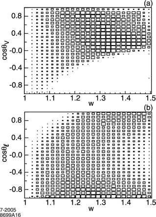
Six bins were chosen for the $\chi^{2}$ to make sure we have adequate statistics in each bin while still having sensitivity to the shape predicted by Eq. (II.2) combined with detector and event selection acceptance. The kinematically empty regions shown for Monte Carlo events in Fig. 11a for $w\geq 1.08$ and backward ${\cos\theta_{\ell}}$ (due to the electron momentum cut) and in Fig. 11b for small $w$ and forward ${\cos\theta_{V}}$ (due to slow pion acceptance) are excluded by simple cuts on minimum ${\cos\theta_{\ell}}$ and maximum ${\cos\theta_{V}}$ as functions of $w$, respectively.

Figure 11: Plots showing empty regions (due primarily to cuts) in the phase space of the kinematic variables $w$, ${\cos\theta_{\ell}}$, and ${\cos\theta_{V}}$ using the Monte Carlo sample: (a) shows ${\cos\theta_{\ell}}$ vs. $w$, where the high $w$, low ${\cos\theta_{\ell}}$ region is removed in the goodness-of-fit calculation; (b) shows ${\cos\theta_{V}}$ vs. $w$, the high ${\cos\theta_{V}}$, low $w$ region is removed in the goodness-of-fit calculation.

The $\chi^{2}$ is given by

$$\chi^{2}=\sum_{i}\left(\frac{n_{i}-m_{i}}{\sigma_{\rm dif}}\right)^{2},$$ (51)

where the sum is over the 1296 bins, $n_{i}$ is the number of data events in bin $i$, $m_{i}$ is the weighted number of Monte Carlo events and $\sigma_{\rm dif}$ is the error on the difference $n_{i}-m_{i}$. There is, of course, an error on our estimate of the error $\sigma_{\rm dif}$ too, that makes the $\chi^{2}$ contributions from low statictics bins vary widely. Thus, estimating $\sigma_{\rm dif}$ is critical to obtaining a reasonably behaved $\chi^{2}$ distribution.

Using a simple Monte Carlo simulation divided into 1296 bins that roughly mimics the number of low statistics bins in our dataset, we can achieve a flat $\chi^{2}$ probability distribution if we base the error on the best estimate of the number of events in each bin computed using the overall data-to-Monte-Carlo events ratio $r_{\rm mc}$. That is $m_{i}$ is given by muliplying the number of MC events $n^{\rm mc}_{i}$ by $r_{\rm mc}$.

Specifically, we use $n^{\rm best}_{i}=fn_{i}+(1-f)m_{i}$ where $f\equiv{r_{\rm mc}}/{(1+r_{\rm mc})}$. The difference error $\sigma_{\rm dif}$ is obtained by using $\sqrt{n^{\rm best}_{i}}$ for the contribution from the data and by scaling the error on $m_{i}$ by $\sqrt{n^{\rm best}_{i}/m_{i}}$. Thus, we use the hypothesis we are testing (that the weighted Monte Carlo follows the same distribution as the data) to obtain the best possible estimate of $\sigma_{\rm dif}$ by using the best estimators we can obtain for the number of data events ($n^{\rm best}_{i}$) and for the number of MC events ($n^{\rm best}_{i}/r_{\rm mc}$) to estimate their respective contributions to the error. This procedure reduces the number of bins where the error estimate fluctuates low leading to artificially high $\chi^{2}$ contributions.

For the baseline fit we find

$$\chi^{2}=1336.66$$ (52)

for 1292 degrees-of-freedom (1296 bins minus three free parameters and one for normalization), which yields a $\chi^{2}$ probability of $19\%$ indicating the fitted parameters yield a good description of the full four-dimensional distribution of the data (note that we keep two decimal significant digits in $\chi^{2}$ since every one unit change in correponds to a full one sigma shift in the fit parameter).

VIII.2 One-dimensional Binned Projection Plots

For a more detailed examination of how well we fit the data, we turn to one-dimensional projection plots. Fig. 12 shows the weighted Monte Carlo (histogram) overlaid on the background-subtracted data. The backgrounds are subtracted in the one-dimensional analog to the method used in the fit, as detailed in Sec. VI.3.

The difference divided by its error (“pull”) is shown below each plot. The agreement is very good. The $\chi^{2}$ and the corresponding probability for each variable is summarized in Table 4. We take the number of degrees-of-freedom ($n_{\rm dof}$) to be the number of bins minus one for purposes of estimating the probabilities.

To test our sensitivity to the interference terms in Eq. (II.2) we make the same kind of comparisons in six bins of the angle $\chi$ for the variables ${\cos\theta_{\ell}}$ and ${\cos\theta_{V}}$. Since the normalization is not fixed in these plots the number of degrees-of-freedom is 20. The ${\cos\theta_{\ell}}$ plots are shown in Fig. 13. The ${\cos\theta_{V}}$ plots are in Fig. 14. In Table 5 we collect the $\chi^{2}$ and its probability for each plot. Again the agreement is excellent indicating that the fit succeeds well in reproducing the details of the distribution.

In these plots we can also see the effect of isolating specific portions of the PDF – e.g., in the very low $\chi$ region, $\cos\chi\mbox{$\rightarrow$}1$ and we obtain the modulation effect of the ${\sin\theta_{V}}{\cos\theta_{V}}$ in the fifth term of the PDF, seen in the top left plot in Fig. 14. On the other hand, in the high $\chi$ region, $\cos\chi\mbox{$\rightarrow$}-1$ and this effect flips sign due to the sixth term, as can be clearly seen in the bottom right plot. (These types of effects also occur in Fig. 13 but they are masked by the effect of the $p^{*}_{\ell}$ cut, which suppresses the low ${\cos\theta_{\ell}}$ region strongly in that case, so the modulations are more difficult to observe). Much of the information content of our data is encoded in the interference terms, so it is important to ensure that we reproduce their effect accurately.

Table 4: $\chi^{2}$ and $\chi^{2}$-probability for kinematic variable projections and electron momentum. The number of bins in these histograms is either 20 or 16.

.

variable	$\chi^{2}$/$n_{\rm dof}$	$\chi^{2}$ probability
$w$	22.0/19	28%
${\cos\theta_{\ell}}$	23.0/19	24%
${\cos\theta_{V}}$	31.8/19	3.3%
$\chi$	13.0/19	84%
$p^{*}_{\ell}$	17.3/19	57%
$p_{t}$	9.0/15	88%

Table 5: $\chi^{2}$ and $\chi^{2}$-probability for ${\cos\theta_{\ell}}$ and ${\cos\theta_{V}}$ overlay plots in six bins of the kinematic variable $\chi$. These values correspond to the numerical evaluation of one-dimensional $\chi^{2}$ of Figs. 13 and 14.

variable	$\chi$ cut	$\chi^{2}$/$n_{\rm dof}$	$\chi^{2}$ probability
${\cos\theta_{\ell}}$	$0\leq\chi\leq\frac{\pi}{6}$	18.4/20	56%
${\cos\theta_{\ell}}$	$\frac{\pi}{6}\leq\chi\leq\frac{2\pi}{6}$	19.3/20	50%
${\cos\theta_{\ell}}$	$\frac{2\pi}{6}\leq\chi\leq\frac{3\pi}{6}$	29.6/20	7.7%
${\cos\theta_{\ell}}$	$\frac{3\pi}{6}\leq\chi\leq\frac{4\pi}{6}$	17.9/20	59%
${\cos\theta_{\ell}}$	$\frac{4\pi}{6}\leq\chi\leq\frac{5\pi}{6}$	23.9/20	25%
${\cos\theta_{\ell}}$	$\frac{5\pi}{6}\leq\chi\leq\pi$	12.4/20	90%
${\cos\theta_{V}}$	$0\leq\chi\leq\frac{\pi}{6}$	19.5/20	49%
${\cos\theta_{V}}$	$\frac{\pi}{6}\leq\chi\leq\frac{2\pi}{6}$	26.7/20	14%
${\cos\theta_{V}}$	$\frac{2\pi}{6}\leq\chi\leq\frac{3\pi}{6}$	10.8/20	95%
${\cos\theta_{V}}$	$\frac{3\pi}{6}\leq\chi\leq\frac{4\pi}{6}$	20.1/20	45%
${\cos\theta_{V}}$	$\frac{4\pi}{6}\leq\chi\leq\frac{5\pi}{6}$	27.4/20	12%
${\cos\theta_{V}}$	$\frac{5\pi}{6}\leq\chi\leq\pi$	25.3/20	19%

Figure 12: Background-subtracted data (points) overlaid on Monte Carlo (histograms) for all four kinematic variable distributions and for the electron momentum ($p^{*}_{\ell}$) and transverse momentum ($p_{t}$) of the slow pion for our best fit. In the bottom panel of each figure is shown the pull (difference over error) plot. The red line in the pull plot is not a fit, but is the line at zero shown for comparison (similarly for all following pull plots).

Figure 13: Background-subtracted data (points) overlaid on Monte Carlo (histograms) and pull plots for ${\cos\theta_{\ell}}$ for six $\chi$ cuts.

Figure 14: Background-subtracted data (points) overlaid on Monte Carlo (histograms) and pull plots for ${\cos\theta_{V}}$ for six $\chi$ bins. These plots illustrate our sensitivity to interference effects.

IX Systematic Studies

The systematic uncertainties on the three parameters $R_{1}$, $R_{2}$ and $\rho^{2}$ of the baseline fit (see Sec. II.3) are summarized in Table 7. The systematic errors are comparable for fits which include variation in $w$ of $R_{1}$ and $R_{2}$, such as those shown in Sec. X.

A major source of systematic error arises from the MC simulation, specifically, from the modeling of the detector resolution and efficiency. We are particularly concerned with the efficiency for reconstructing the low-momentum charged pion from $D^{*+}$ decays.

Further, how well the background event generation is modeled, e.g. how close the branching fractions in the event generator are to measured ones, affects the distribution of background we subtract. The kinematic-variable dependence of the backgrounds, however, is not taken from the Monte Carlo but is measured in the data under the assumption that the difference between the Monte Carlo and the data can be represented by a linear kinematic-variable dependence. The uncertainty in this measurement also contributes to the systematic errors. We are also able to check our background estimates using the goodness-of-fit as shown in Section VIII.

Our systematic errors fall broadly into two categories:

• A: Detector simulation, i.e., the accuracy with which the Monte Carlo reproduces the resolution and efficiency of the detector. We are most sensitive to how well it models the complex process of detecting and measuring low-momentum pions.

• B: Simulation of $B$ decays and background, i.e., the accuracy with which our event generation models the signal and background distributions and how well we correct for differences between data and Monte Carlo.

IX.1 Detector Simulation

Extensive studies of the simulation of the detector response, including careful examination of track reconstruction and particle identification efficiencies, have been performed using selected data control samples. Adjustments for known simulation deficiencies are used in investigating and evaluating the systematic errors. Form-factor measurements are insensitive to overall normalization errors. Thus differences in the efficiencies that are independent of the fit variables do not affect the results, but MC/data differences that vary as a function of these variables are of concern.

To assess the uncertainties due to differences in shape rather than normalization (Sec. IX.1.2–Sec.IX.2.1), we vary the efficiency corrections, reweight the Monte Carlo samples with these modified corrections, and rerun the fit to the kinematic variable data. Finally, we take the difference between the results of these fits and those obtained with the nominal Monte Carlo simulation as an estimate of the systematic error on the parameters. This procedure is repeated for each source of detector-based systematic uncertainty. The individual uncertainties are added in quadrature to obtain the total systematic error.

IX.1.1 Charged Particle Identification (PID)

Using data and Monte Carlo simulated control samples we have studied the difference in particle identification efficiency $\varepsilon_{pid}$ between data and Monte Carlo. We calculate a correction factor, $\varepsilon^{(data)}_{pid}/\varepsilon^{(mc)}_{pid}$ , as a function of momentum. For electrons the correction factors vary from 0.991 to 1.008 over the momentum range from $1.2{\mathrm{\,Ge\kern-1.00006ptV\!/}c}$ to $2.5{\mathrm{\,Ge\kern-1.00006ptV\!/}c}$. We assess the impact of the uncertainty in these corrections by approximating their momentum dependence by linear functions and varying the size of the small slope of these functions by its one-sigma uncertainty. The observed deviations from the default fit are $\Delta R_{1}=0.0064$, $\Delta R_{2}=0.0052$ and $\Delta{\mbox{$\rho^{2}$}}=-0.0016$ for the increased slope and $-0.0032$, $-0.0031$, $+0.0009$ for the decreased slope. We take half of the difference as the systematic error from this source. Since the momentum dependence is not a monotonic function, this procedure slightly overestimates the uncertainty.

For kaon identification we employ the same procedure. The observed variations are significantly smaller.

The probability of misidentifying the charged hadrons $\pi^{\pm}$, $K^{\pm}$, $p^{\pm}$, as electrons is small, less than $0.2\%$ in the momentum range $1.2-2.5{\mathrm{\,Ge\kern-1.00006ptV\!/}c}$. Since a variation of the peaking background by 9% results in a very modest change in the fit results, and since the fraction of this background originating from hadrons misidentified as electrons is small, we conclude that the uncertainty in the hadron misidentification rate is negligible.

The misidentification rate of pions as kaons as a function of pion momentum ranges from a few tenths of a percent to almost $5\%$. However, pion misidentification is well simulated by the Monte Carlo and thus should have little impact on the fit results. Furthermore, the main consequence of pion misidentification is to increase the combinatorial background. Since we estimate the combinatorial background from a fit to the measured $\Delta m$ distribution, we are not dependent on the Monte Carlo to assess the size of this background. We conclude that the uncertainty in the pion misidentification rate has little impact on the fit results.

IX.1.2 Charged Particle Tracking

The difference between data and Monte Carlo for the tracking efficiency for electrons, charged kaons and pions decreases roughly linearly as a function of momentum. Analogously to the method described for the PID error of Sec. IX.1.1, we vary this linear dependence on the particle momentum in the Monte Carlo simulation and take the small deviation as the error from this source. It is a small contribution to the total systematic error.

IX.1.3 Slow Pion Reconstruction

The efficiency for reconstructing the low-momentum charged pion ($\pi_{s}$) from the decay $D^{*+}\mbox{$\rightarrow$}\mbox{$D^{0}$}\mbox{$\pi_{s}$}$ is a major source of systematic error. Because of the small energy release in $D^{*}$ decays, this pion is emitted in approximately the same direction as the parent $D^{*}$ and its momentum in reconstructed events varies from approximately 50 to 400 ${\mathrm{\,Me\kern-1.00006ptV\!/}c}$ in the laboratory frame, peaking at $\sim 100{\mathrm{\,Me\kern-1.00006ptV\!/}c}$, and with a long tail extending out to 400 ${\mathrm{\,Me\kern-1.00006ptV\!/}c}$. Since $w=E_{D^{*}}/m_{D^{*}}$ in the $B$ rest frame, the $\pi_{s}$ momentum is correlated with $w$ and thus its momentum-dependent efficiency impacts especially the measurement of $\rho^{2}$.

The uncertainty due to the low-momentum tracking efficiency is evaluated differently from other tracking errors because such low-momentum tracks do not traverse the whole drift chamber. Their detection and measurement depends primarily on the silicon vertex tracker. To study this efficiency as a function of $p_{\pi_{s}}$ we use a large sample of $D^{*+}\rightarrow D^{0}\pi_{s}^{+}$ decays selected from all events and measure the distributions of the helicity angle of $\pi_{s}^{+}$ ($\theta_{\pi_{s}})$ in the $D^{*+}$ rest frame as a function of the $D^{*+}$ momentum.

We parameterize the $\pi_{s}$ efficiency as function of its momentum using the form

$$\varepsilon(p_{\pi_{s}})=\varepsilon_{\rm max}\left(1-\frac{1}{1+\beta(p_{\pi_{s}}-p_{0})}\right)$$ (53)

with $p_{0}$ being the threshold momentum and $\beta$ controlling the rapidity with which the efficiency rises above threshold. For $p_{\pi_{s}}<p_{0}$ we set $\varepsilon$ to zero. We fit the data and Monte Carlo helicity angle distributions for $\beta$, $p_{0}$ and the coefficient of the $\cos^{2}\theta_{\pi_{s}}$ term (allowed because the $D^{*}$ is in general polarized to varying degrees in each momentum bin, see Sec. V.2) to obtain efficiency functions for the data and the Monte Carlo. The helicity method only determines the relative momentum dependence of the efficiency. The absolute dependency is not relevant for this analysis.

To assess the systematic uncertainty due to the $\pi_{s}$ efficiency ($\varepsilon(p_{\mbox{$\pi_{s}$}})$) we weight the Monte Carlo simulation by the ratio of the data function to the Monte Carlo function and assign the observed shifts in the fitted values for $R_{1}$, $R_{2}$ and $\rho^{2}$ as systematic errors. As expected, $\rho^{2}$ is the most sensitive ($\Delta{\mbox{$\rho^{2}$}}=0.018$) to $\varepsilon(p_{\mbox{$\pi_{s}$}})$ since, of all the kinematic variables, $\varepsilon(p_{\mbox{$\pi_{s}$}})$ most strongly affects the shape of the $w$-distribution, which is the kinematic variable that has the strongest impact on the extracted $\rho^{2}$ value.

IX.2 Event Simulation

IX.2.1 Final State Radiation

Final state radiation, primarily from electrons in the decay chain, lowers the momenta and to a lesser degree changes the angles of detected particles. Though a physics effect, final-state radiation acts much like a resolution – it smears the kinematic variables. We simulate the emission spectrum of radiative photons using PHOTOS Was , so the resolution-efficiency correction procedure properly corrects for final-state radiation to the extent that PHOTOS models it correctly.

To test the sensitivity to uncertainty in the simulation of final-state radiation we evaluate the shifts in the fitted values of $R_{1}$, $R_{2}$ and $\rho^{2}$ between fits done with and without final-state radiation corrections. We assume an uncertainty of 30% in the simulated photon emission and thus take $\sim 1/3$ of the observed shifts (final-state radiation on vs. final-state radiation off) of $0.0129$, $0.0067$ and $0.0039$ as an estimate of the systematic uncertainty.

IX.2.2 Peaking Background Mixture Uncertainty

The modeling of the peaking background depends on the knowledge of the branching fractions for the mixture of semileptonic $B$ decay modes that make up this background. These branching ratios and the form factors for these modes are not very well measured. To estimate the uncertainty associated with these branching fractions, we use a one-sigma variation of the procedure discussed in Section VI.3, viz.: we first fit the $\cos\theta_{BY}$ distributions with a sum of functions where the signal fraction and the contribution due to the ${D^{**}}$ background are allowed to float. This fit is done in five equal-sized bins for each kinematic variable, over the full kinematically allowed range of the variable, in both data and Monte Carlo. We then take data-to-Monte Carlo ratios of the fit results per bin (shown in Fig.(10)), which we then fit to a linear function of the kinematic variables. While for the central value we use this function to weight the $D^{**}$ background itself before it is subtracted from the data, for the error we vary the weighting function up and down by its one-sigma slope uncertainty as shown in Table 2. The difference of the original fit minus the result of this fit gives us an estimate of the error due to the uncertainty in the shape of the ${D^{**}}$ background for each kinematic variable. We add the uncertainties for each kinematic variable in quadrature to give us the total error due to this source.

Another technique of estimating the $D^{**}$ background error is to vary the branching fractions of the P-wave $D$ meson and non-resonant mode components while keeping the overall peaking background fixed. The results of using this technique come out to be of a similar scale to using the above method, which relies on fits to data. Using both techniques would double-count the error, so we rely on the data-fit technique alone to estimate the error from this source.

IX.2.3 Combinatorial Background Shape Uncertainty

A procedure similar to that employed for the peaking background shape is used to estimate the impact of the uncertainty on the shape of the combinatorial background, except in this case we work with the $\Delta m$ fits rather than the $\cos\theta_{BY}$ fits. As before, we do this fit in five equal-sized bins for each kinematic variable over the full kinematically allowed range of the variable, in both data and Monte Carlo. We then take data-to-Monte Carlo ratios of the fit results per bin, and find the results shown in Fig.(9), which we then can approximate with linear fits. We use these fit results with their associated one-sigma slope uncertainties shown in Table 1 to weight the combinatorial background fraction up and down and fit to the data minus this reweighted distribution. The difference from the original fits gives us an estimate of the error due to the shape of combinatorial background uncertainty for each kinematic variable. Adding the uncertainties for each kinematic variable in quadrature gives us the total error from this source.

IX.2.4 Background Check with Goodness-of-Fit

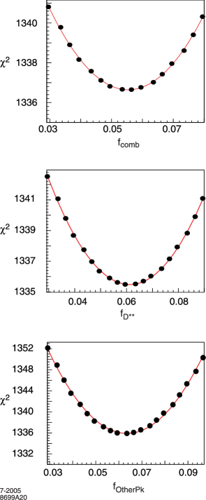
The quality of the fit as measured by the binned $\chi^{2}$ (see Sec. VIII) is sensitive to the background fraction assumed. Thus, we can use $\chi^{2}$ to check our estimate of the backgrounds. Figure 15 shows plots of $\chi^{2}$ versus the fractions of the combinatorial, ${D^{**}}$, and other peaking backgrounds. These scans yield estimates of the background fractions (in percent) of

$$f_{\rm comb}=5.4\pm 1.3,$$

$$f_{D^{**}}=6.1\pm 1.2,$$ (54)

$$f_{\rm otherPk}=6.4\pm 0.9,$$

which are in good agreement with the values of $5.33\%$, $4.85\%$ and $7.03\%$ obtained from the $\Delta m$ and $\cos\theta_{BY}$ fits in section VI.3.

The good agreement indicates not only that the sizes of these backgrounds are well-estimated, but that the shape in the four-dimensional kinematic-variable phase-space given by the Monte Carlo agrees well with their shape in the data.

Figure 15: $\chi^{2}$ of fit vs. fractions of combinatorial ($f_{\rm comb}$), ${D^{**}}$($f_{D^{**}}$) and other peaking backgrounds ($f_{\rm otherPk}$). From this we see that our method of ascertaining the goodness-of-fit is independently indicating that the values we obtained for these fractions from the $\cos\theta_{BY}$ and $\Delta m$ fits were correct.

IX.2.5 Total Peaking and Combinatorial Background Fractions

Another source of error is the uncertainty in the normalization of the peaking and combinatorial background fractions. To estimate this error we vary the fractions $f_{\rm comb}$, $f_{D^{**}}$ and $f_{\rm otherPk}$ by their uncertainties and assess the impact on the fit parameters. The uncertainties for the combinatorial and ${D^{**}}$ fractions are taken from the $\Delta m$ and $\cos\theta_{BY}$ fits. However, since $f_{\rm otherPk}$ is input to these fits by scaling the Monte Carlo distribution, we take its uncertainty instead from the goodness-of-fit scan of the previous section. In varying $f_{\rm otherPk}$ we keep the total peaking $f_{\rm peaking}=f_{D^{**}}+f_{\rm otherPk}$ fixed, since this behavior is observed when $f_{\rm otherPk}$ is varied in the $\cos\theta_{BY}$ fit.

IX.2.6 MC/Data Sideband Comparison

The distributions of the kinematic variables for Monte Carlo and data agree well in the $\Delta m$ sideband region used to estimate the combinatorial background. But since the combinatorial background comprises about a third of the total background under the peak, the small differences in the shapes of the distributions could introduce an error in the background subtraction process. To estimate the impact of this effect, we first take the data-to-Monte Carlo ratios in the sideband region and then fit these ratios with polynomials.

We next use these functions one at a time to multiply the combinatorial background from Monte Carlo before it is subtracted from the data to prepare the sample for fitting. We then carry through the fits and take the differences in the form factors we obtain from these with the form factors we obtained from the fits with the unaltered background. This procedure yields the results shown in Table 6.

The differences are small. The largest is from using the function for ${w}$, from which we find $\Delta\rho^{2}$ $\sim 0.006$. Since in the end we take the $w$-dependence of the combinatorial background from the data and the deviations due to weighting the angular distributions are small, we add nothing to the systematic uncertainty from this check.

Table 6: Changes in the fitted parameters for reweighting of the Monte Carlo combinatorial background distributions in the four kinematic variables.

Reweighted distributions	$R_{1}$	$R_{2}$	$\rho^{2}$
$w$ distribution	$-0.002$	$\hphantom{+}0.0\hphantom{00}$	$\hphantom{+}0.006$
${\cos\theta_{\ell}}$ distribution	$\hphantom{+}0.001$	$-0.002$	$-0.001$
${\cos\theta_{V}}$ distribution	$\hphantom{+}0.002$	$-0.003$	$\hphantom{+}0.001$
${\chi}$ distribution	$\hphantom{+}0.004$	$-0.002$	$\hphantom{+}0.001$

IX.3 Summary of Systematic Errors

The systematic errors are summarized in Table 7. The largest contributions to the systematic errors of $R_{1}$ and $R_{2}$ arise from the uncertainties in background composition, and in the normalization of non-${D^{**}}$ peaking backgrounds. On the other hand, the largest contributions to the systematic error of $\rho^{2}$ arise from the uncertainties in the kinematic variable-dependence of the backgrounds, in the slow pion tracking efficiency and also in the normalization of non-${D^{**}}$ peaking backgrounds.

While the total error remains statistics-dominated, this result is only about a factor of two above the systematic limit. An improved understanding of the systematics would be needed if we were to extend this analysis to other $D$ decay modes and a larger data set.

Table 7: Summary of the estimated systematic errors for the baseline fit.

Error source	$\sigma_{{\mbox{$R_{1}$}}}$	$\sigma_{{\mbox{$R_{2}$}}}$	$\sigma_{{\mbox{$\rho^{2}$}}}$
Charged particle track efficiency	0.005	0.004	0.003
Slow pion track efficiency	0.003	0.000	0.018
PID misID (electron, kaon)	0.006	0.004	0.003
${D^{**}}$ background normalization	0.003	0.002	0.005
Other peaking backgrounds normalization	0.021	0.006	0.015
Combinatorial background normalization	0.002	0.001	0.003
Bkgd composition (branching fractions)	0.016	0.008	0.005
Kinematic Variable-dependence of bkgd	0.001	0.001	0.028
Final state radiation	0.005	0.002	0.002
Total Systematic	0.027	0.013	0.035

X Summary and Discussion

Based on a sample of 16,386 $B^{0}\rightarrow D^{*-}e^{+}\nu_{e}$ events, we have measured the form factors $A_{1}$, $V$ and $A_{2}$ in terms of the HQET-inspired parameters $R_{1}$, $R_{2}$ and $\rho^{2}$. The baseline result, using the CLN parameterization of $h_{A_{1}}(w)$  (see Sec. II.3) is obtained neglecting any possible $w$-dependence of $R_{1}(w)$ and $R_{2}(w)$, and including all errors is

$$R_{1}=1.396\pm 0.060\pm 0.035\pm 0.027,$$

$$R_{2}=0.885\pm 0.040\pm 0.022\pm 0.013,$$ (55)

$$\rho^{2}=1.145\pm 0.059\pm 0.030\pm 0.035,$$

where the first error is statistical, the second Monte Carlo statistical, and the third systematic.

Note that the CLEO result discussed in Sec. I was obtained using the expansion in $(w-1)$ (see Eq. (II.3)) to linear order. When analyzed in this manner, the current dataset yields ${\mbox{$R_{1}$}}=1.40\pm 0.06$, ${\mbox{$R_{2}$}}=0.87\pm 0.04$, and ${\mbox{$\rho^{2}$}}=0.79\pm 0.06$. CLEO also obtained $\rho^{2}$ using the form (see Eq.(13)) suggested by reference oliver that is very close numerically to the CLN parameterization we use. In this case they obtained $\rho^{2}=1.42\pm 0.32$ which is consistent with our result.

The values of $\rho^{2}$ obtained are very different using the linear parameterization, as mentioned in Sec. I. This is because the linear fit significantly underestimates the slope as it attempts to accommodate the higher-order terms (i.e., at $w=1$, the absolute value of the slope is larger assuming a curve for the fit vs. a line).

The $\chi^{2}$ of this linear fit is $1337.98$ which is $1.32$ units of $\chi^{2}$ worse than the baseline fit using the expansion of Eq. (II.3) (see Eq.( 52)). Thus while the baseline fit is slightly better than the linear, both are acceptable.

The sensitivity needed to independently establish the $w$-dependence of $R_{1}(w)$ and $R_{2}(w)$ is not yet available, but theoretical predictions may be used to make comparisons. If we compare the predictions of CLN CLN for $R_{1}(w)$ and $R_{2}(w)$ (see Table 3) to the baseline result, the shifts are found to be $\Delta R_{1}=1.42-1.27=0.15$ ($\approx 2.0\sigma$ apart) and $\Delta R_{2}=0.87-0.80=0.07$ ($\approx 1.5\sigma$ apart). For Ligeti and Grinstein LigetiGrinstein the numbers are $\Delta{\mbox{$R_{1}$}}=1.42-1.25=0.17$ ($2.3\sigma$) and $\Delta{\mbox{$R_{2}$}}=0.87-0.81=0.06$ ($\approx 1.3\sigma$). The older prediction of Neubert NeubertPhysReport is closer with $\Delta R_{1}$ giving $\approx 0.6\sigma$. If the theoretical error on $R_{1}$ is $\sim 0.03$ as estimated by Ligeti ligetipc then there is a mild indication of disagreement. Higher statistics will be needed to resolve or confirm the possible discrepancy.

These results allow a five-fold reduction in the largest source of systematic error in $V_{\rm cb}$ measurements based on $B\rightarrow\mbox{ $D^{*}$}\ell\nu$ decays to be made. Using the measurements of $R_{1}$ and $R_{2}$ presented in this paper, we update the result from the 2004 BABAR paperbabarVcb to find

$$|V_{\rm cb}|=37.6\pm 0.3(stat)\pm 1.3(syst)\hphantom{x}^{+1.5}_{-1.3}(theory)\\ \times 10^{-3}.$$

where small correlations between the present analysis and that of Ref. babarVcb have been ignored. The error due to the uncertainties in $R_{1}$ and $R_{2}$ is reduced from $\hphantom{x}{}^{+2.9\%}_{-2.6\%}$ to $\pm 0.5\%$. The overall systematic error drops from $\pm 1.7$ to $\pm 1.3$. The other systematic errors remain the same as published in Ref. babarVcb .

A considerable improvement was also obtained in measurements of the lepton endpoint spectrum in $b\mbox{$\rightarrow$}u\ell\nu$ decays. Compared to usage of the old CLEO $B\mbox{$\rightarrow$}\mbox{ $D^{*}$}$ form-factor measurements, usage of these newer form factors allowed the systematic error on the inclusive $B\mbox{$\rightarrow$}X_{u}\ell\nu$ branching fraction for decays with a lepton in the momentum range $2.0-2.6{\mathrm{\,Ge\kern-1.00006ptV\!/}c}$ to be reduced from $6.7\%$ to $2.4\%$. In the higher momentum range $2.3-2.6{\mathrm{\,Ge\kern-1.00006ptV\!/}c}$ the improvement was from $2.8\%$ to $1.3\%$. This enabled a significant improvement in the measurement of $|V_{\rm ub}|$ from the endpoint spectrumref:endpt .

In addition we have demonstrated useful approximations to the maximum likelihood method that allow us to cope with the limited size of the Monte Carlo samples available to modern high-luminosity experiments. We have also developed the procedures needed to evaluate the corrections and additional uncertainties due to these approximations. These methods are not unique to $B\mbox{$\rightarrow$}D^{*}\ell\nu$ or $B\mbox{$\rightarrow$}J/\psi K^{*}$ decays, but could be applied to any analysis with a complex multi-dimensional acceptance and resolution functions.

An approach to multi-dimensional goodness-of-fit criteria that allows assessment of the quality of a likelihood fit has also been developed. A binned $\chi^{2}$ measure, with the method developed to estimate the errors, yields a measure of goodness-of-fit that has a straightforward statistical interpretation which is easily and intuitively understandable.

XI Acknowledgments

The authors wish to thank B. Grinstein, Z. Ligeti, M. Neubert, L. Lellouch and L. Oliver for very useful discussions of the theoretical issues involved in this work.

We are grateful for the extraordinary contributions of our PEP-II colleagues in achieving the excellent luminosity and machine conditions that have made this work possible. The success of this project also relies critically on the expertise and dedication of the computing organizations that support BABAR. The collaborating institutions wish to thank SLAC for its support and the kind hospitality extended to them. This work is supported by the US Department of Energy and National Science Foundation, the Natural Sciences and Engineering Research Council (Canada), Institute of High Energy Physics (China), the Commissariat à l’Energie Atomique and Institut National de Physique Nucléaire et de Physique des Particules (France), the Bundesministerium für Bildung und Forschung and Deutsche Forschungsgemeinschaft (Germany), the Istituto Nazionale di Fisica Nucleare (Italy), the Foundation for Fundamental Research on Matter (The Netherlands), the Research Council of Norway, the Ministry of Science and Technology of the Russian Federation, and the Particle Physics and Astronomy Research Council (United Kingdom). Individuals have received support from CONACyT (Mexico), the A. P. Sloan Foundation, the Research Corporation, and the Alexander von Humboldt Foundation.

Appendix A: Evaluation of additional errors

We supply here some of the mathematical details associated with biases and uncertainties introduced in our application of the maximum likelihood method. See Ref. Gill for further details.

Except as noted, in the below, we use the notation of Sec. VI.

.1 Bias From Approximate PDF

Suppose events are distributed as

$$\frac{{\cal F}(x;\mu_{\rm t})}{\int dx{\cal F}(x;\mu_{\rm{}_{t}})},$$ (56)

but the unnormalized PDF used in the maximum likelihood fit is $f(x;\mu)$ (defined by Eq.(30) and used as an approximation for the unknown ${\cal F}(\tilde{x};\mu)$ in Eq. (VI.1.1)). As the number of events $N$ tends to infinity, the sum defining the likelihood can be replaced by the integral

$$\ln L=N\int dx{\cal F}(x;\mu_{\rm t})\ln f(x;\mu)-N\ln\int dxf(x;\mu).$$ (57)

The second term comes from normalizing the PDF. If we expand about $\mu_{\rm t}$ and keep only the leading terms, treating

$$\frac{{\cal F}(x;\mu_{\rm t})}{\int dx{\cal F}(x;\mu_{\rm t})}-\frac{f(x;\mu_{\rm t})}{\int dxf(x;\mu_{\rm t})}$$ (58)

as being itself of order $\mu-\mu_{\rm t}$, we find that the maximum occurs at the point where the derivatives given by

$$\footnotesize\frac{\partial}{\partial\mu}\ln L=\int dx{\cal F}(x;\mu_{t})\frac{\partial}{\partial\mu}\ln f\left(\frac{{\cal F}(x;\mu_{\rm t})}{\int dx{\cal F}(x;\mu_{\rm t})}-\frac{f(x;\mu_{\rm t})}{\int dxf(x;\mu_{\rm t})}\right)+\left(\left<{\frac{\partial\ln f}{\partial\mu}}\right>\left<{\frac{\partial\ln f}{\partial\mu}}\right>^{T}-\left<{\left<\frac{\partial\ln f}{\partial\mu}\right>\left(\frac{\partial\ln f}{\partial\mu}\right)^{T}}\right>\right)(\mu-\mu_{\rm t})$$ (59)

are zero. All derivatives are evaluated at $\mu=\mu_{\rm t}$.

When we take the approximation

$$f(x;\mu)={\cal F}(x;\mu_{\rm mc})\frac{F(x;\mu)}{F(x;\mu_{\rm mc})}$$ (60)

and expand about $\mu=\mu_{\rm t}$, we find to leading order

$$\frac{{\cal F}(x;\mu_{\rm t})}{\int dx{\cal F}(x;\mu_{\rm t})}-\frac{f(x;\mu_{\rm t})}{\int dxf(x;\mu_{\rm t})}=\frac{{\cal F}(x;\mu_{\rm t})}{\int dx{\cal F}(x;\mu_{\rm t})}\left[\langle\frac{\partial\ln\frac{\cal F}{F}}{\partial\mu}\rangle-{\frac{\partial\ln\frac{\cal F}{F}}{\partial\mu}}\right]^{T}(\mu_{\rm mc}-\mu_{\rm t}).$$ (61)

Setting the derivative of the log-likelihood to zero, we have

$$(\mu_{\rm mc}-\mu_{\rm t})\left[\left<{\frac{\partial\ln\frac{{\cal F}}{F}}{\partial\mu}}\right>\left<{\frac{\partial\ln F}{\partial\mu}}\right>^{T}-\left<{\left(\frac{\partial\ln\frac{{\cal F}}{F}}{\partial\mu}\right)\left(\frac{\partial\ln F}{\partial\mu}\right)^{T}}\right>\right]^{T}=$$

$$-(\mu-\mu_{\rm t})\left[\left<{\frac{\partial\ln F}{\partial\mu}}\right>\left<{\frac{\partial\ln F}{\partial\mu}}\right>^{T}-\left<{\left(\frac{\partial\ln F}{\partial\mu}\right)\left(\frac{\partial\ln F}{\partial\mu}\right)^{T}}\right>\right]^{T}.$$ (62)

Solving for the bias $\mu-\mu_{\rm t}$ yields the result Eq.(34).

.2 Error from Monte Carlo evaluation of normalization

The error induced by the use of Monte Carlo integration to normalize a PDF can be calculated considering the asymptotic form

$$\ln L=N\int dxf(x;\mu_{\rm t})\ln f(x;\mu)-N\ln[\int f(x;\mu)dx+\epsilon(\mu)]$$ (63)

where now we are no longer concerned with the distinction between ${\cal F}$ and $f$. The function $\epsilon(\mu)$ is the deviation of the Monte Carlo integral from the true integral. The maximization equation now reads

$$\frac{\partial}{\partial\mu}\ln L=\left(\left<{\frac{\partial\ln f}{\partial\mu}}\right>\left<{\frac{\partial\ln f}{\partial\mu}}\right>^{T}\left<{\left(\frac{\partial\ln f}{\partial\mu}\right)\left(\frac{\partial\ln f}{\partial\mu}\right)}\right>^{T}\right)(\mu-\mu_{\rm t})-\frac{\partial}{\partial\mu}\frac{\epsilon(\mu)}{\int dxf(x;\mu)},$$ (64)

so, again setting the log of the likelihood to zero, the bias is

$$(\mu-\mu_{\rm t})=-\frac{\partial}{\partial\mu}\frac{\epsilon(\mu)}{\int dxf(x;\mu)}E,$$ (65)

where we recognize that the term multiplying $(\mu-\mu_{t}$) in Eq.(64) is the inverse of the error matrix $E$.

Now we suppose the Monte Carlo simulation to be accurate so there is no bias, but an uncertainty is introduced by the fluctuations in $\epsilon$. We therefore need an estimate of the matrix

$$\left<{\left(\frac{\partial}{\partial\mu_{\alpha}}\frac{\epsilon(\mu)}{\int dyf(y;\mu)}\right)\left(\frac{\partial}{\partial\mu}\frac{\epsilon(\mu)}{\int dy^{\prime}f(y^{\prime};\mu)}\right)^{T}}\right>.$$ (66)

A straightforward calculation gives

$$\frac{1}{(\int dxf)^{2}}\int dx\left(\frac{\partial f}{\partial\mu}\right)\left(\frac{\partial f}{\partial\mu}\right)^{T}\hfill$$

$$-\frac{1}{(\int dxf)^{3}}\left[\left(\int dx\frac{\partial f}{\partial\mu}\right)\left(\int dxf\frac{\partial f}{\partial\mu}\right)^{T}+\left(\int dxf\frac{\partial f}{\partial\mu}\right)\left(\int dx\frac{\partial f}{\partial\mu}\right)^{T}\right]$$

$$\qquad\qquad\qquad\qquad+\frac{1}{(\int dxf)^{4}}\left(\int dx\frac{\partial f}{\partial\mu}\right)\left(\int dx\frac{\partial f}{\partial\mu}\right)^{T}\int dxf^{2}.$$ (67)

To apply this to our circumstance where we perform a Monte Carlo integration with points having the density ${\cal F}(x;\mu_{\rm mc})$, we need to make the identifications

$$\frac{1}{N_{MC}}\sum_{i}\ldots\rightarrow\frac{1}{\int dx{\cal F}}\int dx{\cal F}(x;\mu_{\rm mc})\ldots;\quad f\rightarrow\frac{F(x;\mu)}{F(x;\mu_{\rm mc})}.$$ (68)

In the final expressions, we do not need to make the distinctions between $\mu$, $\mu_{\rm mc}$, and $\mu_{\rm t}$ which is only necessary when taking the derivatives with respect to $\mu$. These differences are of higher order. This results in the correspondences

$$\int dxf \rightarrow \int dx{\cal F}(x;\mu_{\rm t})$$ (69)

$$\int dx\frac{\partial f}{\partial\mu} \rightarrow \int dx{\cal F}(x;\mu_{\rm t})\frac{\partial\ln F(x;\mu)}{\partial\mu}=\left<{\frac{\partial\ln F}{\partial\mu}}\right>\int dx{\cal F},{\rm etc.}$$ (70)

where the derivatives are evaluated at $\mu_{\rm t}$

In this way we find

$$\left<{\left(\frac{\partial}{\partial\mu}\frac{\epsilon(\mu)}{\int dyf(y;\mu)}\right)\left(\frac{\partial}{\partial\mu_{\beta}}\frac{\epsilon(\mu)}{\int dy^{\prime}f(y^{\prime};\mu)}\right)^{T}}\right> = \frac{1}{M_{MC}}\left<{\left(\frac{\partial\ln F}{\partial\mu}\right)\left(\frac{\partial\ln F}{\partial\mu}\right)}\right>^{T}-\left<{\frac{\partial\ln F}{\partial\mu}}\right>\left<{\frac{\partial\ln F}{\partial\mu}}\right>^{T}$$ (72)

$$= \frac{1}{M_{MC}}E^{-1}$$

and

$$\left<{\left(\mu-\mu_{\rm t}\right)\left(\mu-\mu_{\rm t}\right)^{T}}\right>=E\frac{1}{M_{MC}}E^{-1}E=\frac{1}{M_{MC}}E,$$ (73)

where $M_{MC}=N_{MC}/N_{data}$ is the ratio between the number of MC events and the number of signal events in the data (the inverse of the $r_{\rm mc}$ used in Sec. VIII). That is to say, the error matrix due to Monte Carlo integration has the same form as that for the statistical error from data, except that it is $1/N_{MC}$ instead of $1/N_{\rm data}$ that enters.

.3 Pseudo-log-likelihood Error

The pseudo-log-likelihood error can be computed from sums over the Monte Carlo sample used in the background subtraction. In this case the weights ($w_{i}$) are those used to weight each type of background to obtain the correct normalization as described in Sec. VI.3 (see Eq. (42)).

We consider a pseudo-log-likelihood

$$\ln\mathchar 28931\relax = \sum_{i(S)}\ln F_{S}(x_{i};\mu)+\sum_{j(B)}\ln F_{S}(x_{j};\mu)$$

$$-\sum_{j^{\prime}(B,MC)}\ln F_{S}(x_{j^{\prime}};\mu)-N_{S}\int dxF_{S}(x;\mu)$$

where the $S$, $B$, and $(B,MC)$ indicate that the sums are over signal events, background events, and background MC events, respectively. Of course we cannot know event-by-event which are signal and which are background events, but for the sum this doesn’t matter. The signal distribution is indicated by $F_{S}(x;\mu)$; the background is $F_{B}(x)$. We expand about $\mu=\mu_{\rm t}$ and set $(\partial/\partial\mu_{\alpha})\ln\mathchar 28931\relax$ to zero to find the background subtraction error $E_{S}$ is given by

$$N_{S}E_{S}^{-1}(\mu-\mu_{\rm t}) = \sum_{i(S)}\frac{\partial}{\partial\mu}\delta\ln F_{S}(x_{i};\mu)$$

$$+\sum_{j(B)}\frac{\partial}{\partial\mu}\delta\ln F_{S}(x_{j};\mu)$$

$$\qquad-\sum_{j^{\prime}(B,MC)}\frac{N_{B}}{N_{MC}}\frac{\partial}{\partial\mu}\delta\ln F_{S}(x_{j^{\prime}};\mu)$$

where

$$\delta\ln F_{S}(x_{i};\mu)=\ln F_{S}(x_{i};\mu)-\frac{\int dxF_{S}(x;\mu_{\rm t})\ln F_{S}(x;\mu)}{\int dxF_{S}(x;\mu_{\rm t})},$$ (76)

and

$$E_{S}^{-1}=\left<{\left(\frac{\partial\ln F_{S}}{\partial\mu}\right)\left(\frac{\partial\ln F_{S}}{\partial\mu}\right)^{T}}\right>_{S}$$

$$-\left<{\frac{\partial\ln F_{S}}{\partial\mu}}\right>_{S}\left<{\frac{\partial\ln F_{S}}{\partial\mu}}\right>_{S}^{T}$$ (77)

where

$$\left<{A}\right>_{S}=\int dxF_{S}(x;\mu_{t})A(x)/\int dxF_{S}(x;\mu_{\rm t})$$ (78)

The fluctuations average to zero, but their squares do not. For example,

$$\sum_{i(S)}\sum_{i^{\prime}(S)}\left(\frac{\partial}{\partial\mu}\delta\ln F_{S}(x_{i};\mu_{\rm t})\right)\left(\frac{\partial}{\partial\mu}\delta\ln F_{S}(x_{i^{\prime}};\mu_{\rm t})\right)^{T}=$$ (79)

$$N_{S}\left[\left<{\left(\frac{\partial\delta\ln F_{S}}{\partial\mu}\right)\left(\frac{\partial\delta\ln\ F_{S}}{\partial\mu}\right)}\right>_{S}^{T}-\left<{\frac{\partial\delta\ln F_{S}}{\partial\mu}}\right>_{S}\left<{\frac{\partial\delta\ln F_{S}}{\partial\mu}}\right>_{S}^{T}\right];$$

$$\sum_{j(B)}\sum_{j^{\prime}(B)}\left(\frac{\partial}{\partial\mu}\delta\ln F_{S}(x_{j};\mu_{\rm t})\right)\left(\frac{\partial}{\partial\mu}\delta\ln F_{S}(x_{j^{\prime}};\mu_{\rm t})\right)^{T}=$$

$$N_{B}\left[\left<{\left(\frac{\partial\delta\ln F_{S}}{\partial\mu}\right)\left(\frac{\partial\delta\ln F_{S}}{\partial\mu}\right)}\right>_{B}^{T}-\left<{\frac{\partial\delta\ln F_{S}}{\partial\mu}}\right>_{B}\left<{\frac{\partial\delta\ln F_{S}}{\partial\mu}}\right>_{B}^{T}\right]$$ (80)

where now

$$\langle A\rangle_{B}=\int dxF_{B}(x;\mu_{t})A(x)/\int dxF_{B}(x;\mu_{\rm t}).$$ (81)

Altogether we find

$$\left<{\left(\mu-\mu_{\rm t}\right)\left(\mu-\mu_{\rm t}\right)^{T}}\right>=\frac{1}{N_{S}}{E_{S}}$$

$$\qquad+\frac{1}{N_{S}}\frac{N_{B}}{N_{S}}\left(1+\frac{N_{B}}{N_{MC}}\right){E_{S}}{E_{B}}^{-1}{E_{S}}.$$

Appendix B: Background estimation

This appendix gives more detail on the background estimation procedures.

.4 Combinatorial background

Figure 16 shows the distribution of ${\Delta m}$ for the data sample on a linear scale. The linear scale is used so the level of combinatorial background can be judged by eye from the tail extending outwards towards the right (the peaking backgrounds are underneath the signal peak here and their levels cannot be distinguished from the data). The combinatorial background appears to be of order $5\%$, but it is hidden under a signal that has substantial tails. It is difficult to distinguish tail from background. To extract the background fraction and estimate the signal this distribution is fit to a set of Gaussians representing the signal and to a threshold function to model the background. To investigate the background shape and the tails of the signal Monte Carlo simulated events are used.

Figure 16: The ${\Delta m}$ data distribution for ${D^{*}}e\nu$ candidates on a linear scale.

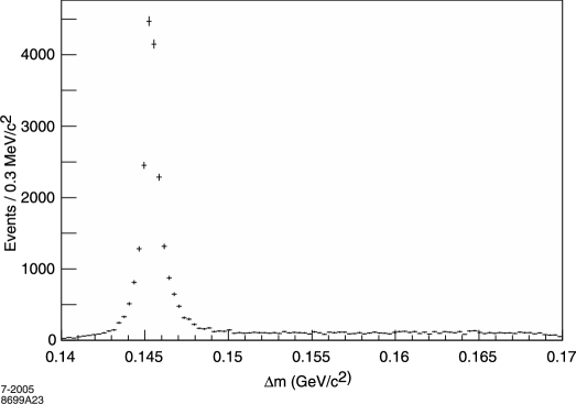
First, to investigate the shape needed to describe the background, a pure combinatorial background sample selected from the Monte Carlo simulation is used.

Figure 17 shows the distribution of Monte Carlo combinatorial background events fit to the (a) unextended (b) and extended threshold function, as discussed in Sec. VI.3.1. Though not immediately obvious by eye, the unextended function systematically underestimates the data in the signal region near ${\Delta m}=0.1454{\mathrm{\,Ge\kern-1.00006ptV\!/}c^{2}}$. The true number in the signal box ($0.143\leq{\Delta m}\leq 0.148{\mathrm{\,Ge\kern-1.00006ptV\!/}c^{2}}$) is 3540. The unextended fit yields $3400\pm 39$ whereas the extended fit yields the much closer result $3528\pm 52$. Fits to subsets of the Monte Carlo data (e.g., those binned in the kinematic variables) show the same pattern with the fit to the extended function having much better success at estimating the number of background events than the unextended.

Next, Figure 18a shows the ${\Delta m}$ distribution of a Monte Carlo simulated pure $D^{*}$ signal sample. There are substantial tails and even the core is not consistent with a single Gaussian. It takes five Gaussians to achieve the good fit shown in Figure 18a.

The fit to the full MC ${\Delta m}$ distribution is finally shown in Figure 18b. In this fit the three core Gaussians of the signal are allowed to float, but the tail is fixed. For the threshold function, the threshold and the scale factor are fixed while the other two parameters are fitted. This procedure reproduces the Monte Carlo input signal and background fractions.

The ${\Delta m}$ distribution of the data with the fit as described is shown in Figure 7. We find $N^{fit}_{cb}=1325\pm 65$ which corresponds to a combinatorial background fraction of $6.4\pm 0.3\%$ before cutting on ${\cos\theta_{BY}}$.

To check the stability of this fit, the fitting conditions are varied. Letting the fourth Gaussian float yields $1374\pm 92$. The error on the difference is $\pm 65$, so this is consistent with the fixed fourth Gaussian used for the central value. Moving the long tail represented by the fifth Gaussian up and down by $50\%$ results in a variation of $\approx\pm 26$ in the background estimate. This variation is added in quadrature with the error reported by the fit to yield a total error of $\pm 70$. The combinatorial background fraction with error becomes $6.39\pm 0.32\%$.

Figure 17: The ${\Delta m}$ distribution for combinatorial background selected from the Monte Carlo with fit to the unextended threshold function (a) and to the extended function.

Figure 18: The ${\Delta m}$ distribution for (a) pure $D^{*}$ signal selected from the Monte Carlo with fit to five Gaussians and (b) the ${\Delta m}$  distributions on the full Monte Carlo sample, fit to the five Gaussian signal shape plus extended threshold function.

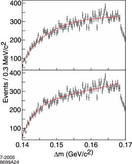
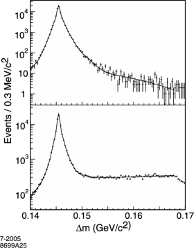
.5 Fits in kinematic variable bins

To estimate the difference in kinematic-variable dependence between data and MC, bin-by-bin fits in five bins for each of the four kinematic variables are done. In the five-bin fits for the combinatorial-background kinematic-variable dependence (as discussed in Sec. VI.3.1) it is found that only four Gaussians are needed to represent the signal shape and that the $\pm 50\%$ variation of the tail Gaussian produces negligible changes in the estimated background level. The ${\Delta m}$ plots with fits are shown in Figure 19. The data-to-Monte Carlo ratio plots which result from these fits is shown Fig. 9 in Section VI.

Figure 19: The ${\Delta m}$ distribution for data in kinematic variable bins. The rows are fits for $w$, ${\cos\theta_{\ell}}$, ${\cos\theta_{V}}$ and $\chi$ in each of the five bins spanning the full range of the variable.

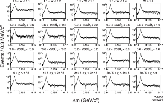
.6 Peaking background including ${D^{**}}$ background fits.

Similarly, $\cos\theta_{BY}$ fits in five bins for each of the four kinematic variables are done to extract the shape of the ${D^{**}}$ background. The results of each fit are shown in Figure 20. The data-to-Monte Carlo ratio used to weight the background obtained from these fits are shown in Figure 10 in Section VI.

Figure 20: The ${\cos\theta_{BY}}$ distributions fit to background plus signal in five bins in each of the kinematic variables. Each row shows the plots for the five bins corresponding to the variables $w$, ${\cos\theta_{\ell}}$, ${\cos\theta_{V}}$ and $\chi$. The shading is the same as that in Figure 10.

References

- (1) J.E. Duboscq et.al. (CLEO Collaboration), Phys. Rev. Lett. 76, 3898 (1996).
- (2) For a theoretical review, see, for example, M. Neubert, “Heavy quark symmetry,” Phys. Rep. 245, 259 (1994) [arXiv:hep-ph/9306320].
- (3) For a review of semileptonic decays, see for example, J. D. Richman and P. R. Burchat, “Leptonic and semileptonic decays of charm and bottom hadrons,” Rev. Mod. Phys. 67, 893 (1995) [arXiv:hep-ph/9508250].
- (4) H. Albrecht et. al. (ARGUS Collaboration), Z. Phys. C 57, 533 (1993).
- (5) D. Buskulic et. al. (ALEPH Collaboration), Phys. Lett. B 359, 236 (1995).
- (6) D. Buskulic et. al. (ALEPH Collaboration), Phys. Lett. B 395, 373 (1997).
- (7) P. Abreu et. al. (DELPHI Collaboration), Phys. Lett. B 510, 55 (2001).
- (8) K. Ackerstaff et. al. (OPAL Collaboration), Phys. Lett. B 395, 128 (1997).
- (9) The BABAR Collaboration, B. Aubert et al., Phys. Rev. D-RC 71, 051502 (2005) [arXiv: hep-ex/0408027].
- (10) I. Caprini, L. Lellouch and M. Neubert, “Dispersive bounds on the shape of form factors,” Nucl. Phys. B 530, 153 (1998) [arXiv:hep-ph/9712417].
- (11) C. G. Boyd, B. Grinstein and R. F. Lebed, “Model independent determinations of form-factors,” Nucl. Phys. B 461, 493 (1996) [arXiv:hep-ph/9508211].
- (12) A. Le Yaouanc, L. Oliver and J. C. Raynal, “Bounds on the derivatives of the Isgur-Wise function from sum rules in the heavy quark limit of QCD,” Phys. Lett. B557, 207 (2003) [arXiv:hep-ph/0210231]; A. Le Yaouanc, L. Oliver and J. C. Raynal, “Sum rules in the heavy quark limit of QCD,” Phys. Rev. D 67, 114009 (2003) [arXiv:hep-ph/0210233].
- (13) N. Isgur and M. B. Wise, “Weak transition form-factors between heavy mesons,” Phys. Lett. B 237, 527 (1990).
- (14) B. Grinstein and Z. Ligeti, “Heavy quark symmetry in spectra,” Phys. Lett. B 526, 345 (2002) [Erratum-ibid. B 601, 236 (2004)] [arXiv:hep-ph/0111392].
- (15) F. E. Close and A. Wambach, “Quark model form-factors for heavy quark effective theory,” Nucl. Phys. B 412, 169 (1994) [arXiv:hep-ph/9307260].
- (16) The BABAR Collaboration, B. Aubert et al., Nucl. Instrum. Methods A 479, 1-116 (2002).
- (17) S. Agostinelli et. al., Geant4 Collaboration, Nucl. Instrum. Methods A 506, 250-302 (2003).
- (18) D. Lange, Nucl. Instrum. Methods A 462, 152-155 (2001).
- (19) A. Ryd, Ph.D. Thesis, University of California, Santa Barbara (UCSB), UMI-97-04221-mc (microfiche), (1996).
- (20) S. Jadach, B. F. L. Ward and Z. Was, “The precision Monte Carlo event generator KK for two-fermion final states in e+ e- collisions,” Comput. Phys. Commun. 130, 260-325 (2000) [arXiv:hep-ph/9912214].
- (21) E. Richter-Was, “QED bremsstrahlung in semileptonic B and leptonic tau decays,” Phys. Lett. B 303, 163 (1993).
- (22) Review of Particle Physics, S. Eidelman et. al., Phys. Lett. B 592, 1 (2004) [http://pdg.lbl.gov].
- (23) “Measurement of the Decay Amplitudes,” by the BABAR Collaboration, Phys. Rev. Lett. 87, 241801 (2001) [arXiv:hep-ex/0107049].
- (24) M. S. Gill, Ph.D. Thesis, University of California, Berkeley (UCB), (2004) [SLAC Report 794: http://www.slac.stanford.edu/cgi-wrap/pubpage?SLAC-R-794].
- (25) The BABAR Collaboration, B. Aubert et al., “Ambiguity-free measurement of : Time-integrated and time-dependent angular analyses of ,” Phys. Rev. D 71, 032005 (2005).
- (26) R. J. Barlow and C. Beeston, “Fitting using finite Monte Carlo samples,” Comput. Phys. Commun. 77, 219 (1993).
- (27) A. Le Yaouanc, L. Oliver and J. C. Raynal, “Lower bounds on the curvature of the Isgur-Wise function,” Phys. Rev. D 69, 094022 (2004) [arXiv:hep-ph/0307197].
- (28) H. Chernoff and E. L. Lehman, Ann. Math. Stat. 25, 579-586 (1954).
- (29) Z. Ligeti, private communication, May 2005.
- (30) The BABAR Collaboration, B. Aubert et al., “Measurement of the inclusive electron spectrum in charmless semileptonic B decays near the kinematic endpoint and determination of V(ub),” to be published in Phys. Rev. D 73, 012066 (2006) [arXiv:hep-ex/0509040].
- (31) “Measurement of Form Factors in the Semileptonic Decay ”, by the BABAR Collaboration, submitted to ICHEP 2004 [arXiv:hep-ex/0409047].