Measurement of the Direct Photon Momentum Spectrum in $\Upsilon({\rm 1S})$, $\Upsilon({\rm 2S})$, and $\Upsilon({\rm 3S})$ Decays

Abstract

Using data taken with the CLEO III detector at the Cornell Electron Storage Ring, we have investigated the direct photon spectrum in the decays ${\Upsilon}({\rm 1S})\to\gamma gg$, ${\Upsilon}({\rm 2S})\to\gamma gg$, ${\Upsilon}({\rm 3S})\to\gamma gg$. The latter two of these are first measurements. Our analysis procedures differ from previous ones in the following ways: a) background estimates (primarily from $\pi^{0}$ decays) are based on isospin symmetry rather than a determination of the $\pi^{0}$ spectrum, which permits measurement of the $\Upsilon$(2S) and $\Upsilon$(3S) direct photon spectra without explicit corrections for $\pi^{0}$ backgrounds from, e.g., $\chi_{bJ}$ states, b) we estimate the branching fractions with a parametrized functional form (exponential) used for the background, c) we use the high-statistics sample of $\Upsilon$(2S)$\to\pi\pi\Upsilon$(1S) to obtain a tagged-sample of $\Upsilon$(1S)$\to\gamma+X$ events, for which there are no QED backgrounds. We determine values for the ratio of the inclusive direct photon decay rate to that of the dominant three-gluon decay $\Upsilon\to ggg$ ($R_{\gamma}=B(gg\gamma)/B(ggg)$) to be: $R_{\gamma}$(1S)=(2.70$\pm$0.01$\pm$0.13$\pm$0.24)%, $R_{\gamma}$(2S)=(3.18$\pm$0.04$\pm$0.22$\pm$0.41)%, and $R_{\gamma}$(3S)=(2.72$\pm$0.06$\pm$0.32$\pm$0.37)%, where the errors shown are statistical, systematic, and theoretical model-dependent, respectively. Given a value of $Q^{2}$, one can estimate a value for the strong coupling constant $\alpha_{s}(Q^{2})$ from $R_{\gamma}$.

Introduction

Production of a $B{\overline{B}}$ meson pair, the Zweig-favored decay mode of $\Upsilon$ mesons, is not energetically possible for resonances below the $\Upsilon$(4S), thus the decay of the $\Upsilon$(1S) meson must proceed through Zweig-suppressed channels. Since the charge conjugation quantum number of the $\Upsilon$ resonances is C=–1, the three lowest-order hadronic decay modes of the $\Upsilon$(1S) meson are those into three gluons ($ggg$), the vacuum polarization QED decay $\Upsilon\to q{\overline{q}}$, and two gluons plus single photon ($gg\gamma$). For the $\Upsilon$(2S) and $\Upsilon$(3S) resonances, direct radiative transitions, both electromagnetic and hadronic, compete with these annihilation modes. Since $\Gamma_{ggg}\propto\alpha_{s}^{3}$ and $\Gamma_{gg\gamma}\propto\alpha_{s}^{2}\alpha_{em},$ the ratio of the decay rates from these two processes can be expressed in terms of the strong coupling constantr:Brod-Lep-Mack :

$$R_{\gamma}\equiv\frac{\Gamma_{gg\gamma}}{\Gamma_{ggg}}=\frac{N_{gg\gamma}}{N_{ggg}}=\frac{38}{5}q_{b}^{2}\frac{\alpha_{em}}{\alpha_{s}}[1+(2.2\pm 0.8)\alpha_{s}/\pi].$$ (1)

In this expression, the bottom quark charge $q_{b}=-1/3$. Alternately, one can normalize to the well-measured dimuon channelr:danko and cancel the electromagnetic vertex: $(\Gamma_{gg\gamma}/\Gamma_{\mu\mu})\propto\alpha_{s}^{2}$.

In either case, one must define the value of $Q^{2}$ appropriate for this process. Although the value $Q^{2}\sim M_{\Upsilon}^{2}$ seems ‘natural’, the original prescription of Brodsky et al.r:Brod-Lep-Mack gave $Q^{2}=(0.157M_{\Upsilon({\rm 1S})})^{2}$ for $\Upsilon$(1S)$\to gg\gamma$.

Theory prescribes the differential spectrum $d^{2}N/dx_{\gamma}d\cos\theta_{z}$ ($x_{\gamma}=p_{\gamma}/E_{\mathrm{beam}}$, and $\cos\theta_{z}$ is defined as the polar angle relative to the $e^{+}e^{-}$ beam axis). The limited angular coverage of the high-resolution CLEO III photon detection, as well as the large backgrounds at low momentum due to decays of neutral hadrons (primarily $\pi^{0}$, $\eta$, $\eta^{\prime}$ and $\omega$) to photons, plus the large number of radiated final state ‘fragmentation’ photons in this regime limit our sensitivity to the region defined by $|\cos\theta_{z}|<$0.7 and $x_{\gamma}>$0.4. We must therefore rely on models for comparison with the observed direct photon spectrum and extrapolation of the direct photon spectrum (excluding the fragmentation component) into lower-momentum and larger polar angle regions.

Originally, the decay of the ground-state vector $b{\overline{b}}$ bottomonium into three vectors (both $\Upsilon\to ggg$ as well as $\Upsilon\to gg\gamma$) was modeled in lowest-order QCD after similar QED decays of orthopositronium into three photons, leading to the expectation that the direct photon spectrum should rise linearly with $x_{\gamma}$ to the kinematic limit ($x_{\gamma}\to 1$); phase space considerations lead to a slight enhancement exactly at the kinematic limitr:lowest-qcd ; r:kol-walsh . Koller and Walsh considered the angular spectrum in detailr:kol-walsh , demonstrating that as the momentum of the most energetic primary parton (photon or gluon) in $\Upsilon\to\gamma gg$ or $\Upsilon\to ggg$ approaches the beam energy, the event axis tends to align with the beam axis: $x_{\gamma}\to 1\Rightarrow dN/d(\cos\theta_{z})\to 1+\cos^{2}\theta_{z}$. Fieldr:Field argued that $x_{\gamma}=1$ is non-physical, since it corresponds to a recoil $gg$ system with zero invariant mass, while the recoil system must have enough mass to produce on-shell final state hadrons. Using a phenomenological parton shower Monte Carlo technique which took into account the correlation of photon momentum with recoil hadronization phase space, Field predicted a significant softening of the lowest-order QCD predicted spectrum, with a photon momentum distribution peaking at $x_{\gamma}\sim 0.65$ rather than $x_{\gamma}\to 1$. (In the limit of completely independent fragmentation, the same argument, in principle, would apply to 3-gluon decays.) This result seemed in conflict with the extant CUSBr:CUSB84 data, which indicated a spectrum more similar to the lowest-order QCD prediction. A subsequent measurement by CLEO-Ir:Csorna , however, favored Field’s softened spectrum over lowest-order QCD. Given the poor resolution of the CLEO-I electromagnetic calorimeter, that measurement was also consistent with a subsequent modification to lowest-order QCD which calculated corrections at the endpointr:Photiadis by summing leading logs of the form ln(1-$x_{\gamma}$). Higher statistics measurements by Crystal Ballr:Bizeti as well as ARGUSr:Albrecht-87 corroborated this softened photon spectrum. A subsequent CLEO analysis (CLEO-II)r:nedpaper , based on $\sim$1 M $\Upsilon$(1S) events, provided a high-statistics confirmation of a photon spectrum peaking at $x_{\gamma}\sim 0.65$, and was able to trace the direct photon momentum spectrum down to $x_{\gamma}\approx$0.4; at that momentum, the direct photon signal becomes less than 10% relative to the background, whereas the systematic errors on the background estimate in that momentum region exceed 10%. Contemporary with the CLEO-II analysis, Catani and Hautmann first pointed out complications due to the presence of fragmentation photons emitted from final–state light quarks downstream of the initial heavy quarkonia decayr:Catani (essentially final state radiation). These can dominate the background-subtracted spectra for $x_{\gamma}<$0.4 and therefore (if not corrected for) lead to an over-estimate of the $\Upsilon$(1S)$\to gg\gamma$ branching fraction, and an underestimate of the extracted value of $\alpha_{s}$.

Hoodbhoy and Yusufr:YusufHoodbhoy96 also performed a rigorous calculation of the expected $\Upsilon$(1S)$\to gg\gamma$ decay rate, by summing all the diagrams contributing to the direct photon final state and treating hard and soft contributions separately. Rather than assuming that the decay occurs via annihilation of two at-rest quarks, the authors smear the annihilation over a size of order $1/m$, with a corresponding non-zero velocity. Although their calculation results in some softening of the photon spectrum relative to the lowest-order QCD prediction, it is unable to entirely account for the softening observed in data, leading to the conclusion that final-state gluon interactions are important, particularly near the photon endpoint.

Fleming and Leibovichr:Fleming03a considered the photon spectrum in three distinct momentum regions. At low momentum ($x_{\gamma}<0.3$), final-state radiation effects dominate. In the intermediate momentum regime (0.3$<x_{\gamma}<$0.7), they applied the operator product expansion (OPE) to the direct photon spectrum of $\Upsilon$ decay, with power-counting rules prescribed by non-relativistic QCD (NRQCD), and retained only the lowest-order color singlet terms in $v/c$. In the highest-momentum regime ($x_{\gamma}>0.7$), a soft-collinear effective theory (SCET) for the light degrees of freedom combined with non-relativistic QCD for the heavy degrees of freedom was used to obtain a prediction for the photon spectrum which qualitatively described the essential features of the CLEO-II data, despite peaking at a higher value of $x_{\gamma}$ than data. The same approach was later applied by Fleming to decays of the type $e^{+}e^{-}\to J/\psi$+X, given the similarity to $e^{+}e^{-}\to\Upsilon$(1S)$\to\gamma$+X, and including the color-octet contributions to $J/\psi$ productionFLM03 .

Very recently, Garcia and Soto (GSr:SotoGarcia04 ) have also produced a parameterization of the expected photon momentum spectrum in the $\Upsilon$ system. Following Fleming and Leibovich, they also remedy the inability of non-relativistic QCD (NRQCD) to model the endpoint region by combining NRQCD with Soft-Collinear Effective Theory, which allows calculation of the spectrum of the collinear gluons resulting as $x_{\gamma}\to 1$. They make their own calculation of the octet contributions (in both S- and P- partial waves) to the overall rate, obtaining a spectral shape prediction similar to Fleming and Leibovich (claimed to be reliable in the interval 0.65$\leq x_{\gamma}\leq$0.92r:GarciaPrivateComm ) after adding color-octet, color-singlet, and fragmentation contributions. For $x_{\gamma}\leq$0.65, Garcia-Soto consider the fragmentation contribution “significant” compared to the direct photon spectrum. For $x_{\gamma}\geq$0.92, the calculation becomes less reliable; in this high-momentum regime, the possibility of two-body decays: $\Upsilon\to gg\gamma\to{\cal X}\gamma$, with ${\cal X}$ some resonant hadronic state, will also lead to distortions of the expected spectrum. Contributions from such possible two-body decays may also result in a slight underestimate of the extracted value of $\alpha_{s}$. Garcia and Soto have also pointed out the possibility of different calculational regimes for $\Upsilon$(1S)$\to\gamma+X$, compared to $\Upsilon$(2S)$\to\gamma+X$ and $\Upsilon$(3S)$\to\gamma+X$, given the difference in the principal quantum numbers, and therefore the average radial interquark separation. Since the Field model is based on simple gluon-gluon fragmentation phase space arguments, it does not distinguish between direct photons from any of the three $\Upsilon$ resonances.

Overview of Analysis

The analysis, in general terms, proceeds as follows. After selecting a high-quality sample of $e^{+}e^{-}$ annihilations into hadrons, we plot the inclusive isolated photon spectrum in data taken at both on-resonance and off-resonance energies. A direct subtraction of the off-resonance contribution isolates the photon spectrum due to $\Upsilon$ decays. The background from decays of neutral hadrons into photons ($\pi^{0}\to\gamma\gamma$, $\eta\to\gamma\gamma$, $\eta^{\prime}\to\rho\gamma$, and $\omega\to\pi^{0}\gamma$) produced in $\Upsilon$ decays to $ggg$, $gg\gamma$, or $q{\overline{q}}$ is removed statistically using a Monte Carlo generator developed specifically for this purpose, and based on the assumption that the kinematics of charged and neutral hadron production can be related through isospin conservation. For each charged pion identified in the data, we simulate a two-body decay of one of the neutral hadrons enumerated above. The measured four-momentum of that charged pion is then used to boost the daughter photons into the lab frame. After correcting for efficiency, and scaling by the expected rate of neutral hadron production relative to charged pion production (for $\pi^{0}$’s, the simple isospin assumption would be $N(\pi^{0})/N(\pi^{\pm})\sim$1/2; for the other neutral hadrons, we use ratios relative to charged pions as derived in our previous analysisr:nedpaper ) and the appropriate branching fractions, a background “pseudo-photon” spectrum is created. After subtracting all backgrounds, the remaining photon spectrum is interpreted as the direct photon spectrum, which must then be extrapolated into low-photon momentum and high $\cos\theta_{z}$ regions (for which the backgrounds are prohibitively large) in order to determine an estimate of the full production rate. In this analysis, we employ the models by Field and Garcia-Soto for integration purposes, given their acceptable match in spectral shape to previous data. Although no predictions exist for direct photon decays of the $\Upsilon$(2S) and $\Upsilon$(3S) resonances, we nevertheless use these same models to determine total direct photon decay rates in the case of these higher resonances. A comparison of the shapes of these models is shown in Figure 1.

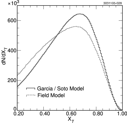
Figure 1: Comparison of the direct photon spectral shapes for the two theoretical models used in this analysis.

Data Sets and Event Criteria

The CLEO III detector is a general purpose solenoidal magnet spectrometer and calorimeter. Elements of the detector, as well as performance characteristics, are described in detail elsewhere r:CLEO-II ; r:CLEOIIIa ; r:CLEOIIIb . For photons in the central “barrel” region of the cesium iodide (CsI) electromagnetic calorimeter, at energies greater than 2 GeV, the energy resolution is given by

$$\frac{\sigma_{\rm E}}{E}(\%)=\frac{0.6}{E^{0.7309}}+1.14-0.01E,$$ (2)

where $E$ is the shower energy in GeV. At 100 MeV, the calorimetric performance is about 20% poorer than indicated by this expression due to the material in front of the calorimeter itself. The tracking system, Ring Imaging Cerenkov Detector (RICH) particle identification system, and electromagnetic calorimeter are all contained within a 1 Tesla superconducting coil.

Event Selection

The data used in this analysis were collected on the $\Upsilon$(1S) resonance, center-of-mass energy $E_{\mathrm{C}M}=9.46$ GeV, the $\Upsilon$(2S) resonance, center-of-mass energy $E_{\mathrm{C}M}=10.02$ GeV, and the $\Upsilon$(3S) resonance, center-of-mass energy $E_{\mathrm{C}M}=10.36$ GeV. In order to check our background estimates, we used continuum data collected just below the $\Upsilon$(1S) resonance, center-of-mass energy $9.431$ GeV $<E_{\mathrm{C}M}<9.434$ GeV, below the $\Upsilon$(2S) resonance, center-of-mass energy $9.996$ GeV $<E_{\mathrm{C}M}<10.004$ GeV, below the $\Upsilon$(3S) resonance, center-of-mass energy $10.329$ GeV $<E_{\mathrm{C}M}<10.331$ GeV and below the $\Upsilon$(4S) resonance, center-of-mass energy $10.41$ GeV $<E_{\mathrm{C}M}<10.57$.

To obtain a clean sample of hadronic events, we selected those events that had a minimum of four high-quality charged tracks (to suppress contamination from QED events), a total visible energy greater than 15% of the total center-of-mass energy (to reduce contamination from two-photon events and beam-gas interactions), and an event vertex position consistent with the nominal $e^{+}e^{-}$ collision point to within $\pm 5$ cm along the $e^{+}e^{-}$ axis (${\hat{z}}$) and $\pm$2 cm in the transverse ($r-\phi$) plane. We additionally veto events with a well-defined electron or muon, or consistent with a $\tau\tau$ “1-prong vs. 3-prong” charged-track topology. Our full data sample is summarized in Table I.

DataSet	Resonance	${\cal L}$ (${\rm pb}^{-1}$)	HadEvts	$\sigma^{had}_{obs}$ (nb)	EvtSel (raw)
1S-A	$\Upsilon$(1S)	6.351	128019	20.16	226746
1S-B	$\Upsilon$(1S)	633.399	12803279	20.21	15720815
1S-C	$\Upsilon$(1S)	424.668	8742850	20.59	10553140
2S-A	$\Upsilon$(2S)	450.907	4165745	9.24	6561803
2S-B	$\Upsilon$(2S)	6.133	55834	9.10	76208
2S-C	$\Upsilon$(2S)	199.665	1839390	9.21	2748240
2S-D	$\Upsilon$(2S)	248.473	2299910	9.26	2914640
2S-E	$\Upsilon$(2S)	283.890	2629250	9.26	3473320
3S-A	$\Upsilon$(3S)	382.902	2482170	6.52	3887570
3S-B	$\Upsilon$(3S)	607.122	3948690	6.50	5736980
3S-C	$\Upsilon$(3S)	180.758	1168980	6.47	2108220
1S-CO-A	$<\Upsilon$(1S)	141.808	485790	3.43	619060
1S-CO-B	$<\Upsilon$(1S)	46.600	159959	3.43	260599
2S-CO-A	$<\Upsilon$(2S)	153.367	472071	3.08	624505
2S-CO-B	$<\Upsilon$(2S)	106.409	326371	3.07	465939
2S-CO-C	$<\Upsilon$(2S)	32.153	99377	3.09	138898
2S-CO-D	$<\Upsilon$(2S)	59.783	183897	3.08	256185
2S-CO-E	$<\Upsilon$(2S)	44.635	137083	3.07	191205
3S-CO-A	$<\Upsilon$(3S)	46.906	135069	2.88	193749
3S-CO-B	$<\Upsilon$(3S)	78.947	226700	2.87	321169
3S-CO-C	$<\Upsilon$(3S)	32.064	91997	2.87	130021
4S-CO-A	$<\Upsilon$(4S)	215.604	594662	2.76	847875
4S-CO-B	$<\Upsilon$(4S)	558.442	1536020	2.75	2189720
4S-CO-C	$<\Upsilon$(4S)	270.896	753418	2.78	1073410
4S-CO-D	$<\Upsilon$(4S)	656.261	1815920	2.77	2587650
4S-CO-E	$<\Upsilon$(4S)	238.903	660883	2.77	941162
4S-CO-F	$<\Upsilon$(4S)	338.620	938454	2.77	1337990

Table 1: Summary of data used in analysis. Different running periods are designated by capital roman letters. For each data set, we track the number of photons per unit luminosity, as well as the total number of observed hadronic events per unit luminosity; consistency of our results across datasets is later used as part of our systematic error assessment. EvtSel denotes events analyzed, HadEvts denotes the total number of events in each sample identified as hadronic by our event selection requirements, and $\sigma$ is the corresponding observed hadronic cross-section for each data sample.

Determination of $N_{gg\gamma}$

To obtain $N_{gg\gamma}$, we had to determine the number of direct photon events. Then, with the number of three-gluon events, we can extract the ratio $R_{\gamma}$. For $N_{gg\gamma}$, only photons from the barrel region ($|\cos\theta_{z}|<0.7$) were considered. Photon candidates were required to be well-separated from charged tracks and other photon candidates, with a lateral shower shape consistent with that expected from a true photon. Photons produced in the decay of a highly energetic $\pi^{0}$ would sometimes produce overlapping showers in the calorimeter, creating a so-called ‘merged’ $\pi^{0}$. Two selection requirements were imposed to remove this background. First, any two photons which both have energies greater than 50 MeV and also have an opening angle $\theta_{\gamma_{1}\gamma_{2}}$ such that $\cos\theta_{\gamma_{1}\gamma_{2}}>$0.975 are removed from candidacy as direct photons. Second, an effective invariant mass was determined from the energy distribution within a single electromagnetic shower. Showers with effective invariant masses consistent with those from merged $\pi^{0}$’s were also rejected. After all photon and event selection requirements, the momentum-dependent direct-photon finding efficiency is shown in Figure 2, as calculated from a large-statistics sample of photon showers simulated with the standard, GEANT-based CLEO III detector simulation. We note that, since the minimum charged multiplicity requirement dominates the efficiency near the upper endpoint, the $\Upsilon$(2S)$\to gg\gamma$ and $\Upsilon$(3S)$\to gg\gamma$ direct-photon finding efficiencies $\epsilon(x_{\gamma})$ are higher than those shown for the $\Upsilon$(1S), given their higher initial center-of-mass energies. Our final branching fraction calculations explicitly correct for this photon momentum dependence.

Figure 2: Efficiency for an event containing a fiducially contained direct photon to pass both event selection and shower selection requirements for $\Upsilon$(1S)$\to\gamma gg$ using our default photon selection requirements and our default charged multiplicity requirement ($\geq$4 charged tracks observed in a candidate event; solid); $\Upsilon$(1S)$\to\gamma gg$ showing the efficiency if the multiplicity requirement was relaxed to $\geq$2 charged tracks (dashed); $\Upsilon$(1S) direct-photon daughters, for $\Upsilon$(1S) produced in $\Upsilon$(2S) dipion decays (dotted, and discussed later in this document). Efficiencies are derived from full GEANT-based CLEO III detector simulations.

Using GEANT-based CLEO III detector simulations, we have compared the shower-reconstruction efficiency (not imposing event selection requirements) for direct photons with the shower-reconstruction efficiency for well-separated photons produced in the decay $\pi^{0}\to\gamma\gamma$; these efficiencies are observed to agree to within 3% over the momentum region of interest (Fig. 3). The photon spectrum inferred from the observed charged pion spectrum is “multiplied” by the dashed line in this figure to estimate the background photons expected from the decay of neutral pions produced in gluon and quark fragmentation.

Figure 3: Comparison of shower-reconstruction efficiency for direct photons, compared to well-separated photons resulting from $\pi^{0}$ decays, based on full GEANT-based CLEO III simulations. The former efficiency is used to determine final direct photon signal branching fractions in the data itself; the latter is used to determine the fraction of generated pseudo-photons which are expected to contribute to the background showers observed in data. The difference between the two is attributed to the typically greater isolation of direct photons.

The dominant backgrounds to the direct photon measurement are of two types: initial state radiation ($x_{\gamma}>0.65$) and the overwhelming number of background photons primarily from asymmetric $\pi^{0}$ decays ($x_{\gamma}<$0.65), that result in two, spatially well-separated daughter photons which elude the $\pi^{0}$ suppression described above. If our Monte Carlo generator were sufficiently accurate, of course, we could use the GEANT-based CLEO III Monte Carlo simulation itself to directly generate the expected background to the direct photon signal, including all background sources. We have compared this GEANT-derived photon spectrum (based on the JETSET 7.4 event generator) with data for continuum events at $E_{\mathrm{CM}}=10.55$ GeV. We observe fair, but not excellent agreement between the two, motivating a data-driven estimate of the background to the direct photon signal. We use GEANT to model the response of the calorimeter to photon showers (Fig. 2), but use the data itself as an event generator of three-gluon decays, in place of JETSET. To model the production of $\pi^{0}$ daughter photons, we took advantage of the similar kinematic distributions expected between charged and neutral pions, as dictated by isospin invariance. Although isospin conservation will break down at low center-of-mass energies (where, e.g., the neutral vs. charged pion mass differences and contributions from weak decays may become important), at the high-energy end of the spectrum (provided there is sufficient phase space), we expect isospin conservation to be reliable, so that there should be half as many neutral pions as charged pions. We stress here that this is true for three-gluon decays, $\chi_{bJ}$ decays, ${\it I}=0$ continuum $q{\overline{q}}$ events, ${\it I}=0$ $e^{+}e^{-}\to\Upsilon\to\gamma^{\star}\to q{\overline{q}}$ events, etc.

There are, nevertheless, both ‘physics’ as well as detector biases which comprise corrections to our isospin assumption, as follows. For continuum production of hadrons via $\gamma^{\star}\to(u{\overline{u}}+d{\overline{d}})$, the ratio of ${\it I}=1/{\it I}=0$ production is expected to be 9:1. Particles with ${\it I}$=0 ($\omega$, $f_{0}$, etc.) should decay in accordance with our naive assumption that $\pi^{0}/\pi^{\pm}$=1/2. For sufficiently high-multiplicity decays, such that all $\rho$ states are populated evenly, we again expect $\pi^{0}/\pi^{\pm}$=1/2; very close to the threshold turn-on, phase space effects will favor $\rho^{0}$ production, in which case $\pi^{0}/\pi^{\pm}<$1/2. Our explicit subtraction of the photon spectrum obtained on the continuum will remove any such biases from $e^{+}e^{-}\to\gamma^{\star}\to q{\overline{q}}$, leaving three-gluon decays as the primary background source, which are presumed to obey isospin conservation.

Acceptance-related biases, which will affect both continuum as well as resonance decays, include: a) slight inefficiencies in our charged $\pi^{\pm}$ identification and tracking, b) charged kaons and protons which fake charged pions, and c) for low multiplicity events, an enhanced likelihood that an event with charged pions will pass our minimum charged-multiplicity requirement compared to an event with neutral pions. The $\pi^{0}/\pi^{\pm}$ ratio therefore deviates slightly from 0.5, as a function of momentum. Figure 4 shows the (JETSET+GEANT)-based neutral to charged pion production ratio for continuum $e^{+}e^{-}\to q{\overline{q}}(\gamma)$ events taking into account such selection biases; we observe agreement with the 0.5 expectation to within 3%. For this study, we rely on JETSET 7.4 to produce the proper ratio of $\pi^{0}:\pi^{\pm}$ at the generator level in hadronic $\Upsilon$ fragmentation, if not the individual spectra themselves. In our analysis, we use this ratio, rather than the simple isospin expectation, to generate pseudo-$\pi^{0}$’s using data charged pions as input. The deviation between this value and the simple isospin expectation is later incorporated into the overall systematic error.

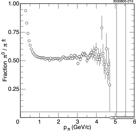
Figure 4: $\pi^{0}/({\pi^{+}}+{\pi^{-}})$ ratio, as a function of charged pion momentum, including tracking efficiency, particle identification efficiency and event selection requirements (from GEANT-based CLEO III Monte Carlo simulations). The loss of efficiency at large $p_{\pi}$ is largely due to the bias introduced by the minimum charged-particle multiplicity requirement.

These pseudo-$\pi^{0}$’s are subsequently decayed according to a phase space model, and the resulting simulated photon spectrum is then plotted. It includes our GEANT-derived photon efficiency, and the correlation between daughter photon momenta and the photon emission direction relative to the $\pi^{0}$ flight direction in the lab. In addition to $\pi^{0}$’s, we also simulate $\eta\rightarrow\gamma\gamma$, $\omega\rightarrow\pi^{0}\gamma$, and $\eta^{\prime}\rightarrow\gamma(\rho,\omega,\gamma)$ contributions, using previous measurements of these backgrounds in $\Upsilon$(1S) decaysr:nedpaper . An estimate of the relative contribution of these various backgrounds to the observed continuum spectrum is shown in Figure 5.

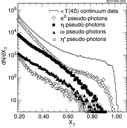
Figure 5: Estimate of the momentum-dependent contribution from various background sources to the observed below-$\Upsilon$(4S) inclusive photon spectrum, based on the JETSET 7.4 event generator plus a full CLEO III GEANT-based detector simulation. Initial state radiation contributions are not included.

We have also studied the relative contribution to the inclusive spectrum from neutrons, anti-neutrons, and $K^{0}_{L}$’s. According to Monte Carlo simulations, the expected numbers of such particles per hadronic event with $|\cos(\theta_{z})|<0.7$, and scaled momentum $x>$ 0.25 (i.e., particles which could populate our signal region) are quite small. Figure 6 gives the yield per event, as a function of momentum, for $K^{0}_{L}$ and anti-neutrons to contaminate our signal region.

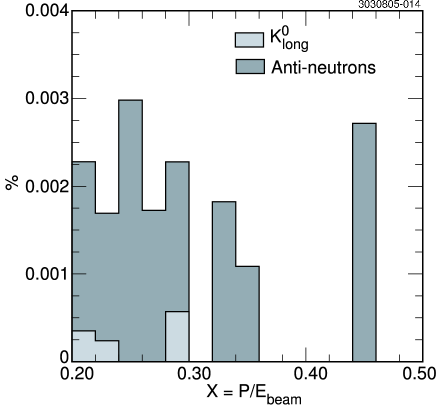
Figure 6: Estimate of the momentum dependent percentage of showers produced by $\bar{n}^{0}$’s and $K^{0}_{L}$’s that passed our shower selection, based on a sample of 1 million MC continuum events. There are no entries for $x>0.5$.

Such contributions are therefore neglected in the remainder of the analysis.

The performance of our photon-background estimator can be calibrated from data itself. Three cross-checks are presented below: a) comparison between the absolutely normalized angular distribution of our simulated pseudo-photons (“PP”) using continuum charged tracks as input to our pseudo-photon generator versus the photon spectrum measured on the continuum (including a Monte Carlo-estimated initial state radiation (“ISR”) contribution (Figure 7)), b) comparison of the absolute magnitude of the pseudo-photon momentum spectrum with continuum data (Figure 8), and c) comparison of the reconstructed $\pi^{0}$ and $\eta$ mass peaks (Figure 9) between our simulated photons and real data photons. All these checks show acceptable agreement between simulation and data. The numerical accuracy of our background estimate can be assessed by comparing, for the second of these checks, the fractional excess remaining after the estimated pseudo-photon background (+ISR) is subtracted from the raw continuum data spectrum, in the momentum interval of interest: $(N_{\mathrm{data}}-N_{\mathrm{pseudo-photons}}-N_{\rm ISR})/N_{\mathrm{data}}$. Integrated from $x_{\gamma}$=0.4 to $x_{\gamma}$=0.95, we find the fractional excesses to be -1.86%, -0.68%, 2.55% and 1.76%, using data below the $\Upsilon$(1S), $\Upsilon$(2S), $\Upsilon$(3S) and $\Upsilon$(4S) resonances, respectively; we consider these excesses to be acceptably consistent with zero.

Other systematic checks of our data (photon yield per data set, comparison between the below-$\Upsilon$(1S), below-$\Upsilon$(2S), below-$\Upsilon$(3S) and below-$\Upsilon$(4S) continuum photon momentum spectra) indicate good internal consistency of all data sets considered.

Figure 7: Angular distribution of the inclusive photons from continuum data compared with our pseudo-photon estimate, based on isospin invariance, for showers with $x_{\gamma}>0.45$, and including a Monte Carlo-based estimate of the ISR background. The normalization is absolute.

Figure 8: Comparison of $x_{\gamma}$ spectra, obtained using below-$\Upsilon$(4S) data, with the sum of ISR Monte Carlo simulations plus a pseudo-photon spectrum obtained using identified data charged pions as input.

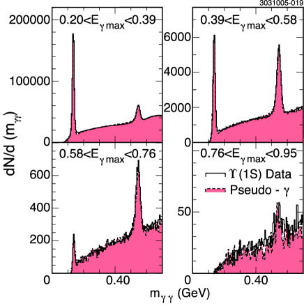
Figure 9: The $\pi^{0}$ and $\eta$ yields for data (dashed) and simulated photons (solid). The yields agree at the 2%-3% level.

Signal Extraction

Two different methods were used to subtract background photons and obtain the $\Upsilon$(1S)$\to gg\gamma$, $\Upsilon$(2S)$\to gg\gamma$ and $\Upsilon$(3S)$\to gg\gamma$ spectra. In the first, after explicitly subtracting the continuum photon spectrum from data taken on-resonance, we use the pseudo-photon spectrum to model the background due to $\pi^{0}$, $\eta$, $\eta^{\prime}$ and $\omega$ decay which must be separated from direct photons from $\Upsilon$ decay. In the second method, we used an exponential parametrization of the background to estimate the non-direct photon contribution.

Figure 10 shows the inclusive $\Upsilon$(1S) photon distribution with the different estimated background contributions (continuum photons from all sources and $\Upsilon$ decays of neutral hadrons into photons) overlaid. After subtracting these sources, what remained of the inclusive $\Upsilon$(1S) spectrum was identified as the direct photon spectrum, $\Upsilon$(1S)$\rightarrow gg\gamma$. Figures 11 and 12 show the corresponding plots for the $\Upsilon$(2S) and $\Upsilon$(3S) data, and also indicate the magnitude of the cascade subtraction due to transitions of the type $\Upsilon$(2S)$\to\Upsilon$(1S)+X, $\Upsilon$(1S)$\to\gamma gg$. We use currently tabulated values for $\Upsilon$(2S)$\to\Upsilon$(1S)+X to determine the magnitude of this correction. Monte Carlo simulations of the primary cascade processes, including $\Upsilon$(2S)$\to\pi\pi\Upsilon$(1S) (using a Yanr:Yan distribution for the dipion mass distribution) and $\Upsilon$(2S)$\to\chi_{b}\gamma$, $\chi_{b}\to\gamma\Upsilon$(1S) are used to adjust the shape of our measured $\Upsilon$(1S)$\to\gamma gg$ direct photon spectrum to that expected for the cascade subtraction in order to account for the shifted kinematic endpoint and Doppler smearing of the daughter $\Upsilon$(1S) direct photon spectrum. We assume that the daughter $\Upsilon$(1S) retains the polarization of the parent $\Upsilon$(2S); the direct photon angular distribution is then the same as for direct production and decay of the $\Upsilon$(1S) resonance.

Figure 10: Photon energy spectrum (minimal cuts) for data taken at the $\Upsilon$(1S) resonance energy, with continuum contribution (using CLEO data taken off the resonance, including ISR) and $\Upsilon$ non-direct simulated pseudo-photons (“pp”) resulting from decays of neutral hadrons overlaid.

Figure 11: $\Upsilon$(2S) photon energy spectrum (minimal cuts), with non-direct pseudo-photons, continuum background photons, and the cascade contribution from $\Upsilon$(1S) decays overlaid.

Figure 12: $\Upsilon$(3S) photon energy spectrum (minimal cuts), with non-direct pseudo-photons, continuum background photons, and the cascade contributions from $\Upsilon$(2S) and $\Upsilon$(1S) decays overlaid.

Parametric estimate of background

Observing that the photon spectrum seems to describe an exponential outside the signal region, we attempted to check our pseudo-photon and continuum-subtracted yields against the signal photon yields obtained when we simply fit the background to an exponential in the momentum region below the signal region (comparing the results obtained from fitting $0.2<x_{\gamma}<0.3$ to those obtained using $0.3<x_{\gamma}<0.4$) and then extrapolated to the region $0.4<x_{\gamma}$. Figure 13 shows that this procedure satisfactorily reproduces continuum data below the $\Upsilon$(4S) resonance, verifying that it may be used to generate a rough estimate of the backgrounds.

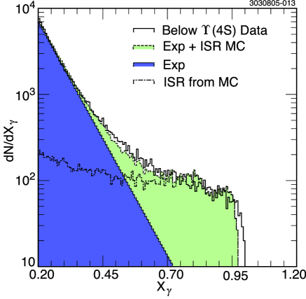
Figure 13: Subtraction of backgrounds using an exponential (below-4S continuum data), with floating normalization to estimate the non-direct photon spectrum. The exponential, plus initial state radiation, gives a fair match to the observed spectrum, although the background is clearly underestimated in the intermediate region of the momentum spectrum.

Model Fits

We estimate $R_{\gamma}$ by extrapolating the background-subtracted photon spectrum down to $x_{\gamma}$=0, using a model to prescribe the spectral shape at low photon momentum. Since the CLEO calorimeter has finite resolution, and since the photon-finding efficiency is momentum-dependent, two procedures may be used to compare with models. Either a migration-matrix can be determined from Monte Carlo simulations to estimate the bin-to-bin smearing, with a matrix-unfolding technique used to compare with prediction, or the model can first be efficiency-attenuated (as a function of momentum) and then smeared by the experimental resolution to compare with data. We have followed the latter procedure, floating only the normalization of the efficiency-attenuated, resolution-smeared model, in this analysis. To determine the percentage of direct photons within our fiducial acceptance, we used the QCD predictions of Koller and Walsh for the direct-photon energy and angular distributionsr:kol-walsh . Our large statistics sample allows (for the first time) a check of the Koller-Walsh prediction. Figure 14

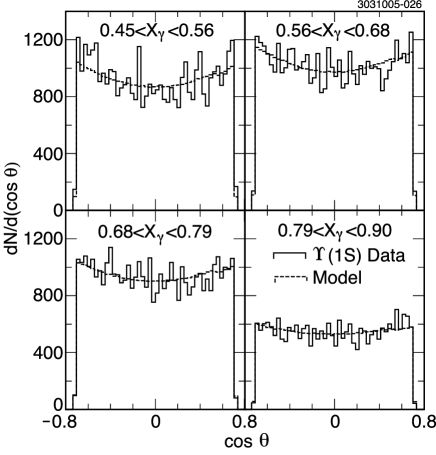
Figure 14: Photon angular distribution for background-subtracted direct photon data (histogram) vs. Koller-Walsh prediction, modified for the experimental efficiency as a function of $x_{\gamma}$ and $\cos\theta_{z}$.

shows that the angular distribution of our data, after taking into account acceptance effects, agrees adequately with the Koller-Walsh prediction.

Figures 15, 16, and 17 show the fits of the direct photon energy spectrum to the Garcia-Soto direct photon model. The fits are performed over the interval claimed to be relatively free of either endpoint effects or fragmentation backgrounds (0.65$\leq x_{\gamma}\leq$0.92), then extrapolated under these backgrounds into the unfit region using only the direct photon component of their spectral model. Field prescribes no such cut-offs, so we have fit that model over the larger kinematic range 0.4$<x_{\gamma}<$0.95. To probe fitting systematics, we have performed two fits. In the first, we perform a simple $\chi^{2}$ minimization of the background-subtracted data to the Garcia-Soto spectrum. In the second, we have normalized the area of the theoretical spectrum to the area of the background-subtracted data in the interval of interest. The two methods yield nearly identical results.

We note, in some cases, an excess of photons in data as $x_{\gamma}\to 1$. Further examination of these events indicate that they are dominated by $e^{+}e^{-}\to\gamma\pi^{+}\pi^{-}\pi^{+}\pi^{-}$.

Figure 15: Fit to background-subtracted $\Upsilon$(1S) data, using explicit continuum data subtraction. Garcia-Soto model is used for spectral shape (modified for efficiency and experimental resolution), either using a $\chi^{2}$ fit in the region where the direct photon contribution dominates, or normalizing the model to the experimental data in the same interval, as shown. The two fits very nearly overlay with each other.

Figure 16: Fit to background-subtracted $\Upsilon$(2S) data, using explicit continuum data subtraction and explicit subtraction of $\Upsilon$(1S) cascade contributions. Direct spectrum fit using Garcia-Soto model.

Figure 17: Fit to background-subtracted $\Upsilon$(3S) data, using explicit continuum data subtraction and explicit subtraction of $\Upsilon$(1S) and $\Upsilon$(2S) cascade contributions.

Figures 18, 19, and 20 show fits obtained using a simple exponential parametrization of the background, with no pseudo-photon generation.

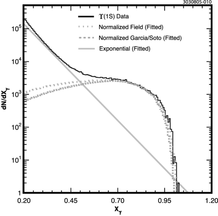
Figure 18: Subtraction of backgrounds using an exponential ($\Upsilon$(1S) data), with floating normalization to estimate the non-direct photon spectrum. Direct spectrum fit using Field model.

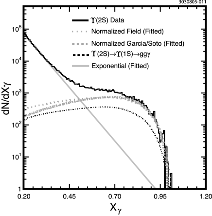
Figure 19: Subtraction of backgrounds using an exponential ($\Upsilon$(2S) data), with floating normalization to estimate the non-direct photon spectrum. Direct spectrum fit using Field.

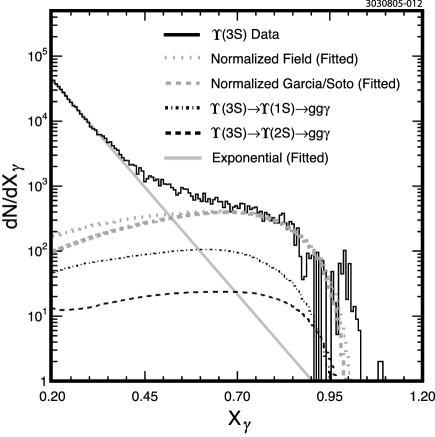
Figure 20: Subtraction of backgrounds using an exponential ($\Upsilon$(3S) data), with floating normalization to estimate the non-direct photon spectrum. Direct spectrum fit using Field.

$\Upsilon$(2S)$\to\pi^{+}\pi^{-}\Upsilon$(1S); $\Upsilon$(1S)$\to\gamma gg$

Our large sample of $\Upsilon$(2S) decays and the substantial $\Upsilon$(2S)$\to\pi^{+}\pi^{-}\Upsilon$(1S) branching fraction ($\sim$0.19) afford an opportunity to measure a ‘tagged’ $\Upsilon$(1S) direct photon spectrum which circumvents all continuum backgrounds. In a given event taken at the $\Upsilon$(2S) center-of-mass energy, we calculate the mass recoiling against all oppositely-signed charged pion pairs (Figure 21).

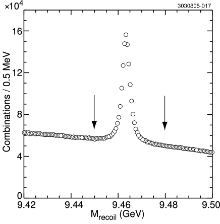
Figure 21: Mass recoiling against oppositely signed charged pion pairs, $\Upsilon$(2S) data.

In each bin of recoil mass, we plot the spectrum of all high-energy photons in that event. A sideband subtraction around the $\Upsilon$(2S)$\to\pi^{+}\pi^{-}\Upsilon$(1S) recoil mass signal, at $m_{\rm recoil}\sim\Upsilon$(1S) results in a tagged $\Upsilon$(1S) direct photon spectrum. Spectral shape and $R_{\gamma}$ values obtained this way are consistent with our other estimates.

Determination of $N_{ggg}$

To determine the number of three-gluon events $N_{ggg}$ from the number of observed $\Upsilon$(1S) hadronic events $N^{\Upsilon({\rm 1S})}_{had}$, we first subtracted the number of continuum events at the $\Upsilon$(1S) energy $N^{\Upsilon({\rm 1S})}_{cont}$ based on the observed number of below-$\Upsilon$(1S) continuum events $N^{E_{\mathrm{C}M}=9.43~{}GeV}_{cont}$:

$$N^{\Upsilon({\rm 1S})}_{cont}=N^{E_{\mathrm{C}M}=9.43~{}GeV}_{cont}\cdot\frac{{\cal L}_{\Upsilon({\rm 1S})}s_{\rm cont}}{{\cal L}_{\rm cont}s_{\rm 1S}}\cdot$$ (3)

where the factor $\frac{{\cal L}_{\Upsilon({\rm 1S})}}{{\cal L}_{\rm cont}}$ arises from the number of events $N={\cal L}\cdot\sigma$, and $s\equiv E_{\mathrm{C}M}^{2}$. From the observed number of hadronic events collected at the resonance $N^{\Upsilon({\rm 1S})}_{had}$, and knowing the branching fractions and efficiencies for $\Upsilon({\rm 1S})\to q{\overline{q}}$, $\Upsilon({\rm 1S})\to gg\gamma$, and $\Upsilon({\rm 1S})\to ggg$, the number of $\Upsilon$(1S)$\to ggg$ events can be inferred. For $\Upsilon({\rm 1S})\to q{\overline{q}}$, e.g., we use the averaged $\Upsilon$(1S)$\rightarrow\mu^{+}\mu^{-}$ branching fraction $B_{\mu\mu}=0.0248$ r:pdg ; r:istvan , and $R_{\Upsilon({\rm 1S})}=\sigma(e^{+}e^{-}\rightarrow\Upsilon$(1S)$\rightarrow q{\bar{q}})/\sigma(e^{+}e^{-}\rightarrow\Upsilon$(1S)$\rightarrow\mu^{+}\mu^{-})=3.51$ r:Albrecht-92 ; r:CLEO-R :

$$N_{q{\overline{q}}}=R_{\Upsilon({\rm 1S})}\cdot B_{\mu\mu}\epsilon_{q{\overline{q}}}\cdot\frac{N^{\Upsilon({\rm 1S})}_{had}}{(1-3B_{\mu\mu}){\overline{\epsilon}}_{had}}$$ (4)

with ${\overline{\epsilon}}_{had}$ the hadronic event reconstruction efficiency, averaged over all hadronic modes, and $\epsilon_{q{\overline{q}}}$ specifically the efficiency for reconstructing an $\Upsilon{\rm(1S)}\to(q{\overline{q}})$ event.

Using ${\cal B}(\Upsilon$(2S)$\to\Upsilon{\rm(1S)}+X$)=(32$\pm$1)%, ${\cal B}(\Upsilon$(3S)$\to\Upsilon{\rm(2S)}+X$)=(10.6$\pm$0.8)%, and ${\cal B}(\Upsilon$(3S)$\to\Upsilon{\rm(3S)}+X$)=(12.1$\pm$0.5)%, three-gluon decay fractions for the three resonances $f_{ggg}$=$81.3\pm 0.5$%, $39\pm 1$%, and $38\pm 1$%, respectively, we obtained a value for $N_{ggg}$ for each of the resonances, based on our measured values for $N_{gg\gamma}$. More details on this subtraction are presented in Table II.

Event Type	Efficiency ($\epsilon$)
$\Upsilon$(1S)$\rightarrow{ggg}$	0.953 $\pm$ 0.003
$\Upsilon$(1S)$\rightarrow{gg\gamma}$	0.751 $\pm$ 0.007
$\Upsilon$(1S)$\rightarrow{q\bar{q}}$	0.871 $\pm$ 0.005
$\Upsilon$(2S)$\rightarrow{ggg}$	0.956 $\pm$ 0.003
$\Upsilon$(2S)$\rightarrow{gg\gamma}$	0.776 $\pm$ 0.007
$\Upsilon$(2S)$\rightarrow{q\bar{q}}$	0.882 $\pm$ 0.005
$\Upsilon$(2S)$\rightarrow\Upsilon$(1S)$+X\rightarrow{ggg}$	0.956 $\pm$ 0.003
$\Upsilon$(2S)$\rightarrow\Upsilon$(1S)$+X\rightarrow{gg\gamma}$	0.778 $\pm$ 0.007
$\Upsilon$(2S)$\rightarrow\Upsilon$(1S)$+X\rightarrow{q\bar{q}}$	0.891 $\pm$ 0.005
$\Upsilon$(2S)$\rightarrow\chi_{bJ}$(1P)$\rightarrow{gg}$ $(J=0,1,2)$	0.933 $\pm$ 0.004
$\Upsilon$(3S)$\rightarrow{ggg}$	0.955 $\pm$ 0.003
$\Upsilon$(3S)$\rightarrow{gg\gamma}$	0.765 $\pm$ 0.007
$\Upsilon$(3S)$\rightarrow{q\bar{q}}$	0.881 $\pm$ 0.005
$\Upsilon$(3S)$\rightarrow\Upsilon$(2S)$+X\rightarrow{ggg}$	0.958 $\pm$ 0.003
$\Upsilon$(3S)$\rightarrow\Upsilon$(2S)$+X\rightarrow{gg\gamma}$	0.765 $\pm$ 0.007
$\Upsilon$(3S)$\rightarrow\Upsilon$(2S)$+X\rightarrow{q\bar{q}}$	0.877 $\pm$ 0.005
$\Upsilon$(3S)$\rightarrow\Upsilon$(1S)$+X\rightarrow{ggg}$	0.961 $\pm$ 0.003
$\Upsilon$(3S)$\rightarrow\Upsilon$(1S)$+X\rightarrow{gg\gamma}$	0.789 $\pm$ 0.006
$\Upsilon$(3S)$\rightarrow\Upsilon$(1S)$+X\rightarrow{q\bar{q}}$	0.90 $\pm$ 0.07
$\Upsilon$(3S)$\rightarrow\chi_{bJ}$(1P)$\rightarrow{gg}$ $(J=0,1,2)$	0.819 $\pm$ 0.006
$\Upsilon$(3S)$\rightarrow\chi_{bJ}$(2P)$\rightarrow{gg}$ $(J=0,1,2)$	0.929 $\pm$ 0.004
$\Upsilon$ Resonance	$N_{\rm total}(\Upsilon$(nS)) $(10^{6})$
$\Upsilon$(1S)	21.0 $\pm$ 0.06
$\Upsilon$(2S)	8.4 $\pm$ 0.04
$\Upsilon$(3S)	5.2 $\pm$ 0.06
Fraction	$f$
$f(\Upsilon$(1S)$\rightarrow{ggg})$	0.813 $\pm$ 0.005
$f(\Upsilon$(2S)$\rightarrow{ggg})$	0.39 $\pm$ 0.01
$f(\Upsilon$(3S)$\rightarrow{ggg})$	0.38 $\pm$ 0.01
$f(\Upsilon$(2S)$\rightarrow\Upsilon$(1S)$+X)$	0.32 $\pm$ 0.01
$f(\Upsilon$(3S)$\rightarrow\Upsilon$(2S)$+X)$	0.106 $\pm$ 0.008
$f(\Upsilon$(3S)$\rightarrow\Upsilon$(1S)$+X)$	0.121 $\pm$ 0.005

Table 2: Efficiencies for the reconstruction of the various types of events considered in this analysis, the total number of calculated $\Upsilon$(1S), $\Upsilon$(2S) and $\Upsilon$(3S) events, and the fractions of these totals which were used to obtain the $\Upsilon\rightarrow{ggg}$ denominator in our measurements of $R_{\gamma}$ (and to scale the direct photon cascade spectra in our $\Upsilon$(2S) and $\Upsilon$(3S) subtractions). These fractions were obtained from the Particle Data Groupr:pdg and include recent CLEO $\chi_{bJ}$ measurementsr:chib . The presented errors on the efficiencies are statistical only. Note that, although there are more possible decay paths from the $\Upsilon$(3S) than the $\Upsilon$(2S), the $ggg$ fractions are comparable owing to the significantly larger $\Upsilon$(2S)$\to\Upsilon$(1S)$\pi\pi$ branching fraction.

Results

With values of $N_{gg\gamma}$ and $N_{ggg}$, the ratio $R_{\gamma}$ can be determined. Table III presents our numerical results for the extracted branching fractions.

$X\to gg\gamma$; $X$=	Background	Field $R_{\gamma}$ / $\chi^{2}$/d.o.f.	GS $R_{\gamma}$ / $\chi^{2}$/d.o.f.
$\Upsilon$(1S)	Exponential	$(2.94\pm 0.02)$% / 115.1/67-1	$(2.39\pm 0.03)$% / 132.4/67-1
$\Upsilon$(1S)	PP (MC ISR)	$(2.81\pm 0.01)$% / 293/74-1	$(2.48\pm 0.01)$% / 694/74-1
$\Upsilon$(1S)	PP (CO ISR)	$(2.93\pm 0.01)$% / 125/67-1	$(2.45\pm 0.01)$% / 116/37-1
$\Upsilon({\rm 2S})\to\pi\pi\Upsilon({\rm 1S})$-tagged	PP (no ISR)	$(2.9\pm 0.3)$% / 118/58-1	$(2.5\pm 0.3)$% / 132/58-1
$\Upsilon$(2S)	Exponential	$(3.7\pm 0.7)$% / 542/105-1	$(3.4\pm 0.4)$% / 773/105-1
$\Upsilon$(2S)	PP (MC ISR)	$(3.42\pm 0.05)$% / 316/67-1	$(3.01\pm 0.04)$% 426/67-1
$\Upsilon$(2S)	PP (CO ISR)	$(3.58\pm 0.05)$% 145/67-1	$(2.77\pm 0.05)$% 87/37-1
$\Upsilon$(3S)	Exponential	$(3.4\pm 0.4)$% 210/105-1	$(3.1\pm 0.1)$% 251/105-1
$\Upsilon$(3S)	PP (MC ISR)	$(2.91\pm 0.07)$% / 263/67-1	$(2.55\pm 0.06)$% 331/67-1
$\Upsilon$(3S)	PP (CO ISR)	$(2.8\pm 0.1)$% / 72/67-1	$(2.1\pm 0.1)$% / 36/37-1

Table 3: Summary of Measurements. “PP” denotes Pseudo-Photon background, “MC ISR” implies that Monte Carlo simulations of initial state radiation were used to subtract the ISR background. These numbers are provided for comparison only and are not used in final averaging, etc. “CO ISR” implies that data ISR was subtracted directly using below-resonance data. Values obtained using an exponential parametrization have had systematic errors (reflecting sensitivity to region chosen for scale normalization of the exponential outside the peak region; for this estimate, branching fractions were compared using the regions $0.2<x_{\gamma}<0.3$ or $0.3<x_{\gamma}<0.4$ to set the scale of the exponential and extrapolate under the signal in the higher-$x_{\gamma}$ region) added in quadrature with the statistical error. All other errors are statistical only. Note that $\Upsilon$(2S) $R_{\gamma}$ values have been corrected for $\Upsilon$(1S)$\to gg\gamma$ contamination; $\Upsilon$(3S) $R_{\gamma}$ values have been corrected for both $\Upsilon$(2S)$\to gg\gamma$, and also $\Upsilon$(1S)$\to gg\gamma$ contamination.

We note that, in general, the reduced $\chi^{2}$ values for the fits tend to be rather high. Structure in the spectrum due to, e.g., two-body radiative decays, may result in such a poor fit and is currently being investigated. The normalization-by-area fits probe the extent to which the model fits may be disproportionately weighted by a small number of points.

Systematic errors

We identify and estimate systematic errors as follows:

1. For the $\Upsilon$(1S), the uncertainty in $N_{ggg}$ is based on the CLEO estimated three-gluon event-finding efficiency uncertainty. For the $\Upsilon$(2S) and $\Upsilon$(3S) decays, the uncertainty in $N_{ggg}$ also folds in uncertainties in the tabulated radiative and hadronic transition decay rates from the parent $\Upsilon$’s, which are necessary for determining $N_{ggg}$ as well as the magnitude of the cascade subtractions. The cascade subtraction errors include statistical ($1\sigma$) uncertainties in the various decay modes of the $\Upsilon$ resonances.

2. Background normalization and background shape uncertainty are evaluated redundantly as follows:

   1. We determine the branching fractions with and without an explicit $\pi^{0}$ veto on the background.

   2. We measure the internal consistency of our results using different sub-samples of our $\Upsilon$(1S), $\Upsilon$(2S) and $\Upsilon$(3S) samples.

   3. Bias in background subtraction can also be estimated using Monte Carlo simulations. We treat the simulation as we do data, and generate pseudo-photons based on the Monte Carlo identified charged pion tracks. After subtracting the pseudo-photon spectrum from the full Monte Carlo photon spectrum, we can compare our pseudo-photon and ISR-subtracted spectrum with the known spectrum that was generated as input to the Monte Carlo detector simulation. For the $\Upsilon$(1S), $\Upsilon$(2S), and $\Upsilon$(3S), we observe fractional deviations of +5.7%, –3.4%, and –2.1% between the input spectrum and the pseudo-photon background-subtracted spectrum. To the extent that the initial state radiation estimate and the photon-finding efficiency are obtained from the same Monte Carlo simulations, this procedure is largely a check of our generation of the pseudo-photon background and the correlation of $\pi^{0}$ decay angle with efficiency.

   4. We extract the direct photon branching fractions using a flat $\pi^{0}:\pi^{\pm}$ isospin ratio of 0.5, compared to the $\pi^{0}:\pi^{\pm}$ ratio based on Monte Carlo simulations, including all our event selection and charged tracking and charged particle identification systematics ($\sim$0.53, Figure 4).

   5. Our uncertainty in the on-resonance vs. off-resonance luminosity scaling, which determines the magnitude of the continuum subtraction is assessed as $<$1%, absolute.

3. Model dependence of the extracted total decay rate is estimated by: i) determining the variation between fits (for a given model) performed using a $\chi^{2}$ minimization prescription, or a simple normalization of area of theoretical spectrum to data, and also by ii) comparing the results obtained from fits to the Field model with results obtained from the fits to the Garcia-Soto model. (We currently assume the Koller-Walsh prescription for the angular distribution is correct, and assign no systematic error for a possible corresponding uncertainty.) The irreducible model-dependence error (the difference between branching fractions obtained with the Field model vs. Garcia-Soto) is presented as the last error in our quoted branching fraction.

There is currently no theoretical consensus on either the shape or magnitude of the fragmentation photon background to the direct photon spectrum. We assign no explicit systematic error to the uncertainty in this component and presume this to be already probed by the variation observed between models, the consistency we observe with results obtained from an exponential fit to the background, and the consistency observed in fitting over different intervals of the background-subtracted spectrum. Given the currently tabulated upper limit on $\Upsilon$(1S)$\to\gamma$+pseudoscalar, pseudoscalar$\to h^{+}h^{-}$ (${\cal B}<3\times 10^{-5}$) and the small branching fractions measured for other two-body exclusive radiative decays (like the $\eta(1440)$, whose dominant modes do not have two charged tracks in the final state), we neglect distortions to the direct photon yield from exclusive two-body decays $\Upsilon\to\gamma+{\cal X}$.

Table IV summarizes the systematic errors studied in this analysis and their estimated effect on $R_{\gamma}$.

Source	$\delta R_{\gamma}(1S/2S/3S)$
Difference (MC Glevel, MC analyzed)	0.08/0.05/0.03
Background Shape/Norm, including:
With/Without a $\pi^{0}$ veto	0.07/0.07/0.07
Isospin Assumption	0.01/0.01/0.01
$\epsilon_{ggg}$	0.08/0.19/0.28
Cascade subtraction	0/0.07/0.14
Luminosity and $\sqrt{s}$ scaling	0.01/0.01/0.01
Fit systematics (norm vs. $\chi^{2}$ fit)	0.01/0.05/0.01
Total Systematic Error	0.13/0.22/0.32
Model Dependence (GS vs. Field)	0.24/0.41/0.37

Table 4: Systematic Errors.

Comparison with previous analyses

Table V compares the results of this analysis with those obtained by previous experiments, in which the number of $\Upsilon$(1S)$\rightarrow gg\gamma$ events were determined using Field’s theoretical model only.

Experiment	$R_{\gamma}(\%)$
CLEO 1.5 ($\Upsilon$(1S))r:Csorna	$2.54\pm 0.18\pm 0.14$
ARGUS ($\Upsilon$(1S))r:Albrecht-87	$3.00\pm 0.13\pm 0.18$
Crystal Ball ($\Upsilon$(1S))r:Bizeti	$2.7\pm 0.2\pm 0.4$
CLEO II ($\Upsilon$(1S))r:nedpaper	$2.77\pm 0.04\pm 0.15$
CLEO III ($\Upsilon$(1S))	$2.70\pm 0.01\pm 0.13\pm 0.24$
CLEO III ($\Upsilon$(2S))	$3.18\pm 0.04\pm 0.22\pm 0.41$
CLEO III ($\Upsilon$(3S))	$2.72\pm 0.06\pm 0.32\pm 0.37$

Table 5: Comparison with other experiments. Errors are statistical, systematic, and model-dependent (Field vs. Garcia/Soto), respectively. Central values are obtained by a direct weighted average (taking into account both statistical and systematic errors, and assuming errors to be uncorrelated, therefore yielding the most conservative estimate of the experimental precision) of the measurements presented in Table III.

Summary

We have re-measured the $\Upsilon$(1S)$\to\gamma gg/\Upsilon$(1S)$\to ggg$ branching fraction ratio ($R_{\gamma}$), obtaining agreement with previous results. We also have made first measurements of $R_{\gamma}$(2S) and $R_{\gamma}$(3S). Our results are, within errors, consistent with the naive expectation that $R_{\gamma}$(1S)$\sim R_{\gamma}$(2S)$\sim R_{\gamma}$(3S), although this equality does not hold for the recent CLEO measurements of $B_{\mu\mu}$ for the three $\Upsilon$ resonancesr:danko . Assuming an energy scale equal to the parent $\Upsilon$ mass, our values of $R_{\gamma}$ for $\Upsilon$(1S)$\to gg\gamma$ (2.70$\pm$0.01$\pm$0.13$\pm$0.24)%, $\Upsilon$(2S)$\to gg\gamma$ (3.18$\pm$0.04$\pm$0.22$\pm$0.41)%, and $\Upsilon$(3S)$\to gg\gamma$ (2.72$\pm$0.06$\pm$0.32$\pm$0.37)% imply values of the strong coupling constant $\alpha_{s}(M_{Z})$ = ($0.1114\pm 0.0002\pm 0.0029\pm 0.0053$), ($0.1026\pm 0.0007\pm 0.0041\pm 0.0077$) and ($0.113\pm 0.001\pm 0.007\pm 0.008$), respectively, which are within errors, albeit consistently lower, compared to the current world average (Appendix I).

*Appendix I) Calculation of strong coupling constant

The decay width $\Upsilon\rightarrow gg\gamma$ has been calculated by Lepage and Mackenzie r:Mack-Lep in terms of the energy involved in the decay process (i.e., $\alpha_{s}(E_{\mathrm{C}M})$, or $\alpha_{s}(M_{\Upsilon}$)):

$$\frac{\Gamma(\Upsilon\rightarrow gg\gamma)}{\Gamma(\Upsilon\rightarrow\mu^{+}\mu^{-})}=\frac{8(\pi^{2}-9)}{9\pi\alpha_{QED}}\alpha_{s}^{2}(M_{\Upsilon})\Biggl{[}1+(3.7\pm 0.4)\frac{\alpha_{s}(M_{\Upsilon})}{\pi}\Biggr{]}.$$ (5)

Sanghera r:Sanghera rewrites this expression in terms of an arbitrary energy (renormalization) scale $\mu$:

$$\frac{\Gamma(\Upsilon\rightarrow gg\gamma)}{\Gamma(\Upsilon\rightarrow\mu^{+}\mu^{-})}=A_{\gamma}\biggl{(}{\alpha_{s}(\mu)\over\pi}\biggr{)}^{2}+A_{\gamma}\biggl{(}{\alpha_{s}(\mu)\over\pi}\biggr{)}^{3}\biggl{[}2\pi b_{0}\ln\biggl{(}{\mu^{2}\over M_{\Upsilon}^{2}}\biggr{)}+(3.7\pm 0.4)\biggr{]},$$ (6)

where $A_{\gamma}={8\pi(\pi^{2}-9)\over 9\alpha_{QED}}$, $b_{0}=(33-2n_{f})/12\pi$, and $n_{f}$ is the number of light quark flavors which participate in the process ($n_{f}=4$ for $\Upsilon$(1S) decays).

Similarly, the decay width $\Upsilon\rightarrow ggg$ has been calculated by Bardeen et al. r:Bardeen and expressed by Lepage et al. r:Brod-Lep-Mack ; r:Mack-Lep-PRL as:

$$\frac{\Gamma(\Upsilon\rightarrow ggg)}{\Gamma(\Upsilon\rightarrow\mu^{+}\mu^{-})}=\frac{10(\pi^{2}-9)}{81\pi e_{b}^{2}}\frac{\alpha_{s}^{3}(M_{\Upsilon})}{\alpha^{2}_{QED}}\Biggl{[}1+\frac{\alpha_{s}(M_{\Upsilon})}{\pi}[(2.770\pm 0.007)\beta_{0}-(14.0\pm 0.5)]+\cdot\cdot\cdot\Biggr{]}$$ (7)

with $\beta_{0}=11-({2\over 3})n_{f}$, and $e_{b}=-{1\over 3}$, the charge of the $b$ quark. Here again Sanghera r:Sanghera uses the same algebraic technique to rewrite this in terms of the renormalization scale:

$$\frac{\Gamma(\Upsilon\rightarrow ggg)}{\Gamma(\Upsilon\rightarrow\mu^{+}\mu^{-})}=A_{g}\biggl{(}{\alpha_{s}(\mu)\over\pi}\biggr{)}^{3}+A_{g}\biggl{(}{\alpha_{s}(\mu)\over\pi}\biggr{)}^{4}\biggl{[}3\pi b_{0}\ln\biggl{(}{\mu^{2}\over M_{\Upsilon}^{2}}\biggr{)}-\biggl{(}{2\over 3}\biggr{)}B_{f}n_{f}+B_{i}\biggr{]}$$ (8)

with $A_{g}={10\pi^{2}(\pi^{2}-9)\over 81e_{b}^{2}}{1\over\alpha_{QED}^{2}}$, $B_{f}=2.770\pm 0.007$, and $B_{i}=16.47\pm 0.58$.

Note that the scale dependent QCD equations (6) and (8) are finite order in $\alpha_{s}$. If these equations were solved to all orders, then they could in principle be used to determine $R_{\gamma}$ independent of the renormalization scale. But since we are dealing with calculations that are finite order, the question of an appropriate scale value must be addressed.

The renormalization scale may be defined in terms of the center of mass energy of the process, $\mu^{2}=f_{\mu}E_{\mathrm{C}M}^{2}$, where $f_{\mu}$ is some positive fraction. Since QCD does not tell us a priori what $f_{\mu}$ should be, we must define the appropriate scale. One possibility would be to define $\mu=E_{\mathrm{C}M}$; that is $f_{\mu}$=1. A number of prescriptions r:Brod-Lep-Mack ; r:Grunberg ; r:Stevenson ; r:Sanghera have been proposed in an attempt to “optimize” the scale. However, each of these prescriptions yields scale values which, in general, vary greatly with the experimental quantity being measured r:Sanghera . We have chosen $f_{\mu}=1$ to facilitate a calculation of $\alpha_{s}$ at each of the $\Upsilon$ resonance energies.

For the $\Upsilon$(1S) analysis, using $\mu=M_{\Upsilon(1S)}$ we find

$$\alpha_{s}(M_{\Upsilon(1S)})=0.1735\pm 0.0005\pm 0.0072\pm 0.0133;$$ (9)

for the $\Upsilon$(2S) analysis, using $\mu=M_{\Upsilon(2S)}$ we find

$$\alpha_{s}(M_{\Upsilon(2S)})=0.151\pm 0.002\pm 0.009\pm 0.017;$$ (10)

for the $\Upsilon$(3S) analysis, using $\mu=M_{\Upsilon(3S)}$ we find

$$\alpha_{s}(M_{\Upsilon(3S)})=0.172\pm 0.003\pm 0.018\pm 0.021.$$ (11)

The errors are statistical, systematic and model-dependent, respectively. These calculations were obtained by finding the zeroes of the ratio of Eqs. 6 and 8 given our measurement of $R_{\gamma}$ for each $\Upsilon$ resonance. The errors were obtained by shifting our measurement of $R_{\gamma}$ by $\pm\sigma$, for each of our three errors, and extracting $\alpha_{s}$ for each relevant error-shifted central value.

These results can then be extrapolated to $\mu=M_{Z}$ using equation 12 r:pdg with $\mu_{0}=M_{\Upsilon}$ for each resonance. For this calculation, only the first three terms of the $\beta$-function were consideredr:ritt .

$$\log{\frac{\mu^{2}}{\mu_{0}^{2}}}=\int^{\alpha_{s}(\mu)}_{\alpha_{s}(\mu_{0})}{\frac{d\alpha}{\beta(\alpha)}}$$ (12)

This calculation for the $\Upsilon$(1S), $\Upsilon$(2S) and $\Upsilon$(3S) results in the following measurements of $\alpha_{s}(M_{Z},\Upsilon({\rm nS}))$:

$$\alpha_{s}^{M_{Z},\Upsilon({\rm 1S})}=0.1114\pm 0.0002\pm 0.0029\pm 0.0053,$$ (13)

$$\alpha_{s}^{M_{Z},\Upsilon({\rm 2S})}=0.1026\pm 0.0007\pm 0.0041\pm 0.0077,$$ (14)

$$\alpha_{s}^{M_{Z},\Upsilon({\rm 3S})}=0.113\pm 0.001\pm 0.007\pm 0.008.$$ (15)

Our results are systematically low compared with the average value of $\alpha_{s}({M_{Z}})=0.119\pm 0.006$ obtained from many variables studied at all the LEP experiments r:pdg , but in better agreement with $\alpha_{s}({M_{Z}})=0.112\pm 0.003$ obtained from an analysis of structure functions in deep inelastic scattering r:Benvenuti and with the previous CLEO measurement of $\alpha_{s}(M_{Z},\Upsilon({\rm 1S}))$ r:nedpaper . For the $\Upsilon$(2S) and $\Upsilon$(3S) measurements, we stress caution in interpreting these results, as it is (again) unclear what procedure should be used to define the renormalization scale.

As an alternative to the extraction method outlined above, the strong coupling constant $\alpha_{s}$ can be written as a function of the QCD scale parameter $\Lambda_{\overline{MS}}$, defined in the modified minimal subtraction scheme (MMSS)r:pdg . Figure 22 presents the contour plot of $\alpha_{s}(\Lambda_{\overline{MS}},~{}f_{\mu}$).

Similarly, the ratio of eqns. (2) and (4) above can be used to eliminate $\alpha_{s}$ and provide a relationship between $R_{\gamma}$, $\Lambda_{\overline{MS}}$, and $f_{\mu}$ (Figure 23).

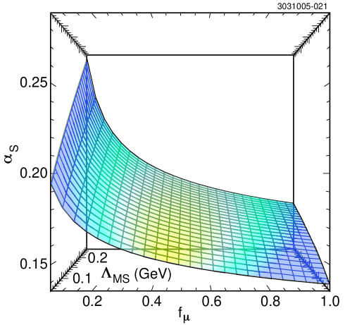
Figure 22: Contour plot illustrating dependence of $\alpha_{s}$ on the QCD scale parameter $\Lambda_{\overline{MS}}$ and the momentum scale $f_{\mu}$.

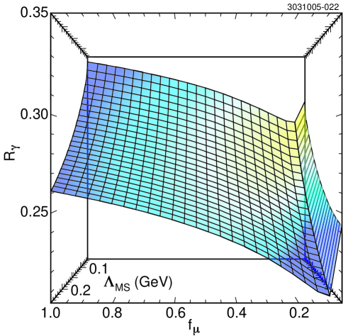
Figure 23: Contour plot illustrating relationship between $R_{\gamma}$, the QCD scale parameter $\Lambda_{\overline{MS}}$ and the momentum scale $f_{\mu}$.

References

- (1) S. J. Brodsky, G. P. Lepage and P. B. Mackenzie, Phys. Rev. D 28, 228 (1983).
- (2) G.S. Adams et al., (CLEO Collaboration), Phys. Rev. Lett. 94, 012001 (2005).
- (3) S.J. Brodsky, T.A.DeGrand, R.R. Horgan and D.G. Coyne, Phys. Lett. B 73, 203 (1978).
- (4) K. Koller and T. Walsh, Nucl. Phys. B140, 449 (1978).
- (5) R.D. Field, Phys. Lett. B133, 248 (1983).
- (6) R.D. Schamberger et al. (CUSB Collaboration), Phys. Lett. B138, 225 (1984).
- (7) S.E. Csorna et al. (CLEO Collaboration), Phys. Rev. Lett. 56, 1222 (1986).
- (8) D.M. Photiadis, Phys. Lett. B164, 160 (1985).
- (9) A. Bizzeti et al. (Crystal Ball Collaboration), Phys. Lett. B267, 286 (1991).
- (10) H. Albrecht et al. (ARGUS Collaboration), Phys. Lett. B199, 291 (1987).
- (11) B. Nemati et al. (CLEO Collaboration), Phys. Rev. D55, 5273 (1997).
- (12) S. Catani and F. Hautmann, Nucl. Phys. B, Proc. Suppl. 39, 359 (1995).
- (13) M. Yusuf and P. Hoodbhoy, Phys. Rev. D54, 3345 (1996).
- (14) S. Fleming and A. Leibovich, Phys. Rev. D67, 074035 (2003); Phys. Rev. Lett. 90, 032001 (2003).
- (15) S. Fleming and A. Leibovich, Phys. Rev. D68 094011, (2003).
- (16) X. Garcia i Tormo and J. Soto, Phys. Rev. D69, 114006 (2004); 72, 054014 (2005); Phys. Rev. Lett. 96, 111801 (2006).
- (17) X. Garcia i Tormo, private communication.
- (18) Y. Kubota et al. (CLEO Collaboration), Nucl. Inst. Meth. A 320, 66 (1992).
- (19) D. Peterson et al., Nucl. Inst. Meth. A 478, 142 (2002).
- (20) M. Artuso et al., Nucl. Inst. Meth. A 502, 91 (2003).
- (21) T. M. Yan, Phys. Rev. D 22, 1652 (1980).
- (22) S. Eidelman it al. (Particle Data Group), Phys. Lett. B 592, 1 (2004) [and 2005 partial update].
- (23) S. B. Athar et al. (CLEO Collaboration), Phys. Rev. Lett. 94, 012001 (2005).
- (24) H. Albrecht et al. (ARGUS Collaboration), Z. Phys. C54, 13 (1992).
- (25) R. Ammar et al., Phys. Rev. D57, 1350 (1998).
- (26) M. Artuso et al., Phys. Rev. Lett. 94, 032001 (2005).
- (27) P. B. Mackenzie and G. Peter Lepage, in Perturbative Quantum Chromodynamics, AIP Conf. Proc., Tallahassee, AIP, New York, (1981).
- (28) S. Sanghera, Int. J. of Mod. Phys. A 9, 5743 (1994).
- (29) W. A. Bardeen et al., Phys. Rev. D 18, 3998 (1978).
- (30) P. B. Mackenzie and G. Peter Lepage, Phys. Rev. Lett. 47, 1244 (1981).
- (31) G. Grunberg, Phys. Lett. B 95, 70 (1980).
- (32) P.M. Stevenson, Phys. Rev. D 23, 2916 (1981).
- (33) S.A. Larin, T. van Ritbergen, and J.A.M. Vermaseren, Phys. Lett. B400, 379 (1997).
- (34) A. C. Benvenuti (BCDMS Collaboration), Phys. Lett B 223, 490 (1989).