Preprint HEN-458
Tests of the Electroweak Sector of the Standard Model

Abstract

The Electroweak sector of the Standard Model is reviewed and best fits are presented for its free parameters based on currently available experimental tests. The Standard Model remains an excellent descriptions of the available experimental data. The preferred mass range of the still elusive Higgs boson in the Standard Model is $114<m_{\mathrm{H}}<219$ GeV at the 95% Confidence Level. A Standard Model Higgs in this mass range is likely to be observed in the years 2007–2010, either at the Tevatron or at the LHC.

Tests of the EW SM  

1 Introduction

The Standard Model (SM) of electroweak [1] and strong interactions [2] is an extremely successful theory that describes the relevant experimental data in detail. In this review we will focus on the electroweak sector of the SM. The strong interaction sector will be discussed in contributions by Greenshaw [3] and Davies [4]. Flavour physics in the quark sector is treated by Branco [5] and Shune [6], while neutrino physics and lepton flavour mixing is covered by Klein [7] and Sanchez [8] in these proceedings.

Despite its elegant principles as a gauge theory the SM is not a trivial structure. Try to write down the Lagrangian after Symmetry breaking [9] ! And this is only part of the story, especially higher orders in perturbation theory make everything connected to everything else.

The hyper charge and weak isospin part of the EW symmetry come with separate couplings strengths, $g^{\prime}$ and $g$. Instead of the coupling strengths $g^{\prime}$ and $g$ other pairs of parameters can also be used, such as the four fermion coupling $G_{F}=g^{2}/4\sqrt{2}M_{\mathrm{W}}^{2}$ and the weak mixing angle $\theta_{w}=\tan^{-1}(g^{\prime}/g)$, or other independent pairs.

There are three ElectroWeak (EW) gauge bosons coupling to fermions: photon to fermions which is purely vector and has strength $g\sin\theta_{w}$, W boson to fermions which is purely vector minus axial-vector with strength $g/2\sqrt{2}$, and Z boson to fermions which is a well defined mix of vector and axial vector couplings with strength $g/2\sin\theta_{w}$. When ignoring the coupling strength, the structure in terms of vector and axial-vector components of the vertices can be written as $\left(v_{Vf}-a_{Vf}\gamma^{5}\right)\gamma^{\mu}$, where I use the symbols $v_{Vf}$ and $a_{Vf}$ for vector and axial-vector coupling coefficients of the vector boson $V$ to fermion species $f$.

In the SM the vector and axial-vector couplings for vector-boson fermion interactions can all be expressed in the charges of the fermions:

$$\begin{array}[]{lll}v_{\gamma f}=Q_{f}&v_{\mathrm{W}f}=T_{3f}&v_{\mathrm{Z}f}=T_{3f}-2Q_{f}\sin^{2}\theta_{w}\\ a_{\gamma f}=0&a_{\mathrm{W}f}=-T_{3f}&a_{\mathrm{Z}f}=-T_{3f}\\ \end{array}\vspace*{-1.5mm}$$

These are the couplings in the Lagrangian and would be the measured couplings if only lowest order effects in the couplings are taken into account. The effective couplings, i.e. those that are measured, include effects of higher orders and become dependent on each other and on all other parameters in the theory, such as masses and charges. Since the relative strength of higher order contributions depend on the distance or energy scale, all these parameters as they are measured will depend on the energy scale at which they are measured.

Where at first sight this may seem nothing but trouble, this notion can also be turned around. Measurements of the SM couplings can be used to predict, e.g. masses of particles, as was successfully done in case of the top quark. Presently such attention goes to the SM Higgs boson mass.

2 Electromagnetic Interactions

The coupling between the photon and fermions is the realm of Quantum ElectroDynamics (QED), which is part of the SM and which is known as the most precise theory around. The QED couplings constant is defined as $\alpha_{\mathrm{QED}}=e^{2}/4\pi=g^{2}\sin^{2}\theta_{w}/4\pi$. Currently one of the major players in the field of SM precision measurements is LEP, with the ALEPH, DELPHI, L3 and OPAL experiments, that collected each about 800 pb^-1 of e⁺e^- data at energies between $m_{\mathrm{Z}}$ and 209 GeV. Also important is the SLD experiment at the SLC with a sample of 350000 Z bosons with polarized beams. Data collection of these experiments has been stopped, the analyses are still ongoing and nearly finished. As we will see, significant inputs to SM tests in the QED sector are also provided by other experiments.

Figure 1: Compton Scattering cross section as measured by the L3 collaboration [11].

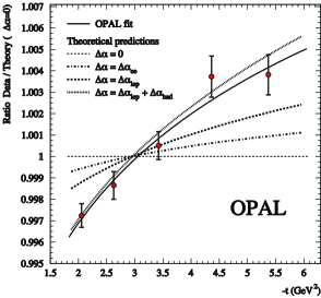
Figure 2: Running of $\alpha_{QED}$ demonstrated by the OPAL collaboration [12]. Plotted is the ratio of the measured interaction strength divided by the expectation without running of the coupling constant.

As a demonstration of the vector character of QED, the Compton scattering (e${}^{\pm}+\gamma$$\rightarrow$e${}^{\pm}+\gamma$) cross section at high energy as measured by L3 and perfectly fitted by the SM is displayed in Fig. 2 [11].

In Fig. 2 the running of $\alpha_{QED}$ is demonstrated at Q² values between 2 and 6 GeV² in the regime of space-like momentum transfer in small angle Bhabha scattering (e${}^{+}+$e^-$\rightarrow$e${}^{+}+$e^-) by the OPAL collaboration [12]. This measurement confirms an earlier L3 measurement [13] with more precision and detail. Although tricky (it is easy to have this measurement make a reference to itself), the running of $\alpha_{QED}$ can be demonstrated over a larger Q² range in the $s$-channel too. In Fig. 4 various measurements from OPAL [12] and L3 [13, 23] are displayed that are reinterpreted using the relation $\alpha_{\mathrm{QED}}(Q^{2})=\alpha_{\mathrm{QED}}(0)/(1-C\,\Delta\alpha_{\mathrm{QED}}(Q^{2}))$ as was done in a contribution to this conference by S. Mele [14].

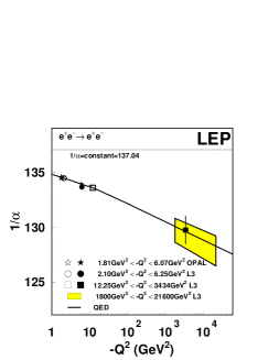
Figure 3: The value of the reciprocal QED coupling constant over a large range of $-Q^{2}$ values. See [14] for further details on this figure.

$(a_{\mu}^{\mathrm{exp}}-a_{\mu}^{\mathrm{SM}})\times 10^{11}$	$\sigma$	Model Ref.
235 (91)	2.6	[15] (e+e-)
221 (108)	2.1	[16] (e+e-)
235 (113)	2.1	[17] (e+e-)
245 (91)	2.7	[18] (e+e-)
225 (81)	2.8	[19] (e+e-)
62 (87)	0.7	[20] ($\tau$)
142 (81)	1.8	[19] (e+e-, $\tau$)

Figure 4: Difference of the muon anomalous magnetic moment predicted the theoretical models indicated in the third column and the measurement [21]. The second column gives the number of standard deviations [22].

The spectacular accuracy of $\alpha_{\mathrm{QED}}(0)=1/137.03599911(46)$ measurement at low $Q^{2}$ values [24] is spoiled when using it to predict the value at higher mass scales, e.g. at the muon or Z mass. In the correction that has to be made for the energy scale dependence: $\alpha_{\mathrm{QED}}^{-1}(Q^{2})=\alpha_{\mathrm{QED}}^{-1}(0)\left(1-\Delta\alpha_{\mathrm{lep}}(Q^{2})-\Delta\alpha_{\mathrm{had}}(Q^{2})\right)$ the hadronic corrections, $\Delta\alpha_{\mathrm{had}}(Q^{2})$, are dominating the uncertainty. At the energy scale corresponding to the Z mass this correction can be expressed as [25]:

$$\Delta\alpha_{\mathrm{had}}(M_{\mathrm{Z}}^{2})=-\frac{\alpha_{\mathrm{QED}}(0)\,s}{3\pi}\int\limits_{s^{\prime}=4m_{\pi}^{2}}^{\infty}\frac{R_{\mathrm{had}}(s^{\prime})}{s^{\prime}(s^{\prime}-M_{\mathrm{Z}}^{2})}\mathrm{d}s^{\prime}+\Delta\alpha_{\mathrm{top}}(M_{\mathrm{Z}}^{2}),\vspace*{-1.5mm}$$

where $R_{\mathrm{had}}(s)$ is the ratio of the e⁺e^- hadronic cross section over $\sigma($e⁺e^-$\rightarrow\mu^{+}\mu^{-})$. In calculating $\Delta\alpha_{\mathrm{had}}$, the measured $R_{\mathrm{had}}(s)$ is used in the five flavour limit for high energy. This is the reason an additional correction for the top contribution has to be made, but this correction is small and theoretically well under control. The most recent result using this technique to estimate the hadronic corrections, and the one preferred by the LEP EW working group, by Burkhardt and Pietrzyk [26], is shown in Fig. 6 and yields $\Delta\alpha_{\mathrm{had}}^{(5)}=0.02758(35)$.

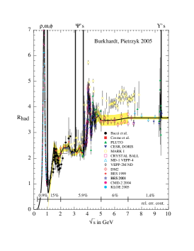
Figure 5: Ratio of hadronic to mu-pair cross section in e⁺e^- annihilation as used in [26] to derive the hadronic correction to the running of $\alpha_{QED}$.

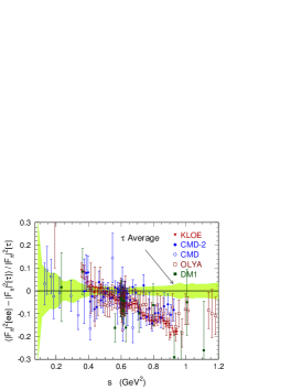
Figure 6: e⁺e^- spectral functions compared to the $\tau$ spectral function as measured by ALEPH, CLEO and OPAL normalised to this $\tau$ spectral function. Figure taken from [27].

It is improved with respect to earlier estimates by using new KLOE [28] data taken at DA$\Phi$NE and CMD-2 [29], SND [30] data taken at VEPP below 1.1 GeV. The uncertainty for the QED coupling constant at the mass of the Z is now dominated by the knowledge of the e⁺e^- annihilation process into hadrons in the $\sqrt{s}$ range from 1.1 to 5 GeV.

The ALEPH collaboration has supplied a paper summarising all its $\tau$ results, including a complete list of exclusive decays and spectral functions [27]. The Belle collaboration also showed $\tau$ results in the parallel session, including a spectral function and a new m_τ measurement [31]. The $\tau$ spectral functions provide another approach to estimate the hadronic corrections to the running of $\alpha_{QED}$. A comparison of e⁺e^- and $\tau$ spectral functions is given in Fig. 6 [27]. This figure shows that there is a discrepancy between the e⁺e^- and $\tau$ spectral functions, which may or may not be due to systematic effects in the theory needed to translate the experimental data into spectral functions. Note however that also the e⁺e^- data from the different experiments are not fully consistent. The uncertainty that is normally assigned to $\alpha_{\mathrm{QED}}$ and the anomalous magnetic moment of the muon, mentioned below, is probably underestimated.

The hadronic correction to the electromagnetic coupling constant is also an important ingredient to the uncertainty on the prediction of the muon anomalous magnetic moment. Translating the knowledge on $\alpha_{\mathrm{QED}}$ into a prediction for $a_{\mu}=(g-2)_{\mu}/2$ we see that the predicted value differs by 0.7 to 2.8 standard deviations from $a_{\mu}=11659214(9)\times 10^{-10}$, the value measured by the Muon $(g-2)$ Collaboration [21] (see Fig. 4.) Clearly more work and data is needed to clear up this situation further.
For the moment there is no reason to think that the SM description is not in correspondence with the data in the QED sector.

3 Weak Interactions

To study the weak interaction the H1 and ZEUS experiments, at the HERA collider have collected some 200 pb^-1 of polarized e⁺ and e^- collision data on protons at $\sqrt{s}=318$ GeV. The total Charged Current (CC) cross section ($\mathrm{ep}\rightarrow\nu\mathrm{X}$) versus $\mathrm{e}^{\pm}$ polarisation plotted in Fig. 7 shows that the exchange of a charged W boson results in a purely vector minus axial-vector coupling.

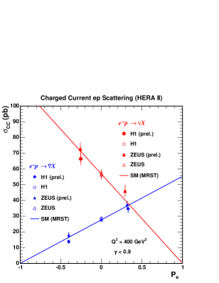
Figure 7: The total charged current cross section for electron-proton and positron-proton scattering at $\sqrt{s}=318$ GeV as a function of polarisation of the lepton beam as measured by the H1 and ZEUS collaborations [32].

For right handed electrons (left handed positrons) the CC cross section becomes zero while it increases linearly with polarisation as expected for a pure $V-A$ coupling.

The H1 collaboration also made a fit to the vector and axial-vector coefficients of the coupling, which is shown in Fig. 8. Although the measurements from LEP [33] and CDF [34] are more precise, only the H1 result [35] is able to distinguish clearly between the two sign ambiguities for both the u and d quark case.

In the first phase of LEP (LEP-1) and at SLD, where data were collected at CM energies near the Z mass, the couplings of the Z boson to fermions were investigated in detail.

The analysis of these data is in its final stages (The final LEP-1 results have been published after this conference in [33]) and most results were not updated for this conference, except for the heavy flavour results that are now all final.

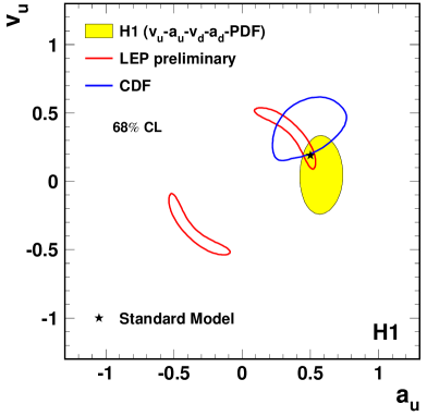
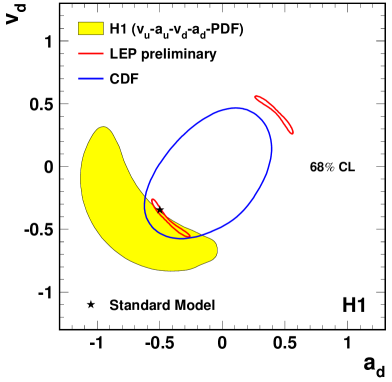
Figure 8: Vector and axial-vector coupling coefficients for u quarks (left) and d quarks (right) as measured by H1 [35], CDF [34] and the LEP experiments [33].

The heavy flavour measurements from the LEP experiments and SLD used in this heavy flavour fit are:

• $R_{q}=\frac{\sigma(\mathrm{e}^{+}\mathrm{e}^{-}\rightarrow\;q\overline{q})}{\sigma(\mathrm{e}^{+}\mathrm{e}^{-}\rightarrow\;\mathrm{hadrons})},\;q=\mathrm{c},\mathrm{b}$, the partial hadronic widths into b and c quarks. The experimental issue is the clean identification of c and b quarks, while the theoretical challenge is to correct for higher order production of heavy quark pairs.

• $A_{\mathrm{FB}}^{0,q}=\frac{\sigma_{\mathrm{F}}-\sigma_{\mathrm{B}}}{\sigma_{\mathrm{F}}+\sigma_{\mathrm{B}}}=A_{\mathrm{e}}A_{q},\;q=\mathrm{c},\mathrm{b}$, the heavy quark forward-backward asymmetries, where the first part of the formula indicates the experimental method, to distinguish the direction of the heavy quark and anti-quark. The direction is called forward (F) if the quark moves in the direction of the incoming electron and backward (B) in the other situation. Theoretically this quantity can be expressed in the product of an asymmetry generated at the Zee, $A_{\mathrm{e}}$ vertex and at the Z$q\overline{q}$ ($q=$c,b) vertex, $A_{q}$.

At SLD also polarised beams are used, which make the measurement of the asymmetries using left- and right-handed polarised beams possible:

• $A_{\mathrm{LR}}^{0}=\frac{\sigma_{\mathrm{L}}-\sigma_{\mathrm{R}}}{\sigma_{\mathrm{L}}-\sigma_{\mathrm{R}}}A_{\mathrm{e}}=\frac{2\,v_{\mathrm{e}}\,a_{\mathrm{e}}}{v_{\mathrm{e}}^{2}+a_{\mathrm{e}}^{2}}$, the left-right asymmetry for the total cross section, where also the relation of this quantity and the coupling coefficients is given. In addition to the considerations given above for heavy flavour measurements, experimentally knowledge of the degree of polarisation of the beams is crucial here. Theoretically the measurement is very clean and many systematic effects, both experimental and theoretical, cancel in asymmetry measurement.

• $A_{\mathrm{LRFB}}^{0,q}=A_{q}=\frac{2\,v_{q}\,a_{q}}{v_{q}^{2}+a_{q}^{2}},\;(q=\mathrm{c},\mathrm{b})$, the combined forward-backward–left-right asymmetry for the total cross section, where also the relation of this quantity and the coupling coefficients is given. The same considerations as in the previous item apply.

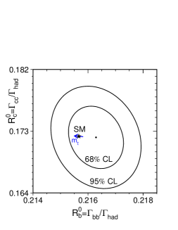
Figure 9: $R_{\mathrm{b}}$ versus $R_{\mathrm{c}}$ from the final LEP EW working group fit to the LEP and SLD heavy flavour data.

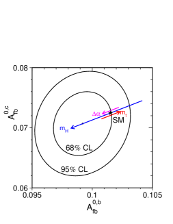
Figure 10: $A_{\mathrm{FB}}^{0,\mathrm{c}}$ versus $A_{\mathrm{FB}}^{0,\mathrm{b}}$ from the LEP EW working group fit to the LEP and SLD heavy flavour data.

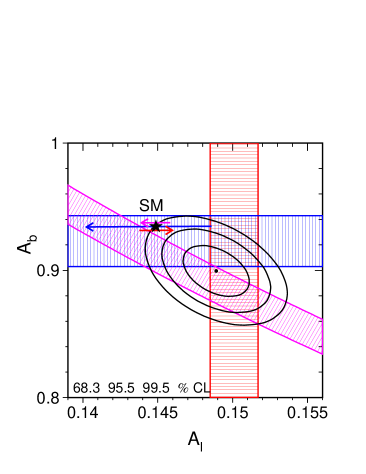
Figure 11: The lepton asymmetry versus b-quark asymmetry. The horizontal and vertical bands are from SLD measurements for $A_{\mathrm{e}}$ and $A_{\mathrm{b}}$. The anti-diagonal is the LEP $A_{\mathrm{FB}}^{(0,b)}$ measurement. The SM prediction is the star, with the influence of $1\sigma$ varying $\Delta\alpha_{\mathrm{had}}$, $m_{\mathrm{H}}$ and $m_{\mathrm{t}}$ indicated by the arrows in top to bottom order.

Figure 12: Electroweak parameter measurements as derived by the LEP EW working group on the basis of ALEPH, DELPHI, L3, OPAL, SLD, CDF and DØ measurements.

Another way to determine the lepton asymmetry is by measuring the $\tau$ polarisation asymmetry $A_{\tau}$, which is done in $\tau$ decays at LEP. In the following the SM relation $A_{\mathrm{e}}=A_{\tau}$ is used.

Combining the heavy flavour measurements from the LEP experiments and SLD and fitting the relevant SM parameters to these measurements a goodness of fit of $\chi^{2}$/d.o.f.$=53/91$ is obtained, indicating excellent overall agreement. This is illustrated in Fig. 10 and 10, which show the measured probability contours for $R_{\mathrm{c}}$ versus $R_{\mathrm{b}}$ and $A_{\mathrm{FB}}^{0,\mathrm{c}}$ versus $A_{\mathrm{FB}}^{0,\mathrm{b}}$ respectively with the SM predictions. The arrows in these figures show the sensitivity to other SM parameters, such as the mass of the top quark, the Higgs boson mass and the size of the hadronic correction to the electromagnetic coupling strength.

Digging a little deeper into all possible comparisons between the measurements and the SM predictions one comes across the situation as depicted in Fig. 12. Although the $A_{\ell}=A_{\mathrm{e}}$ and $A_{\mathrm{b}}$ measurements each agree fairly well with the SM prediction and despite the fact that the measurements agree on a unique $(A_{\mathrm{e}},A_{\mathrm{b}})$ point, there is a discrepancy at the $>3\sigma$ level with the SM prediction for this combination. It should be noted that this is the biggest discrepancy and a single one out of many possible comparisons of the SM to the data.

Apart from the heavy flavour results, the LEP experiments and SLD, produced a number of other parameters at or around a center of mass energy corresponding to the Z boson mass: the mass and width of the Z boson, $m_{\mathrm{Z}}$ and $\Gamma_{\mathrm{Z}}$, the cross section of e⁺e^-$\rightarrow$hadrons, $\sigma_{\mathrm{had}}^{0}$, the ratio of the hadronic to muon-pair final state at the Z peak, $R_{\ell}$, the forward-backward asymmetry for the lepton-pair final state, $A_{\mathrm{FB}}^{0,\ell}$, and the effective lepton weak mixing angle as derived from the forward-backward asymmetry for a Z decaying into quark-pairs using jet-charge techniques, $\sin^{2}\theta_{\mathrm{eff}}^{\mathrm{lept}}(Q_{\mathrm{FB}})$. From running LEP at CM energies above the W-pair threshold also the mass and width of the W boson have been determined, $m_{\mathrm{W}}$ and $\Gamma_{\mathrm{W}}$. The present results as derived by the LEP electroweak working group are listed in Fig. 12. The largest discrepancy in this table is the b quark forward backward asymmetry, which was discussed before.

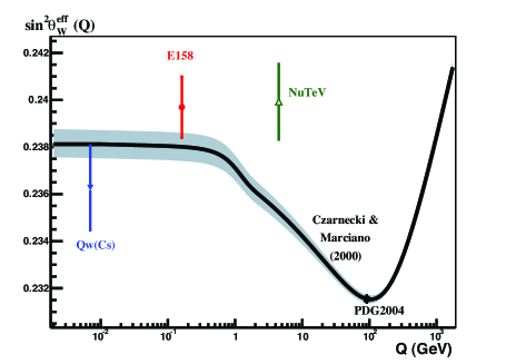
Figure 13: The curve is $\sin^{2}\theta_{w}^{\mathrm{eff}}$ predicted by the SM [36], as a function of $Q=\sqrt{|Q^{2}|}$ when fixed to the value at $Q^{2}=M_{\mathrm{Z}}^{2}$ from [37] based on LEP and SLD measurements. The measurements at $Q\approx 0$ are from atomic parity violation, $Q_{w}$(Cs) [38] and from Møller scattering [39]. At $Q$ values in the range of a few GeV is the neutrino-nucleon scattering result from NuTeV [40].

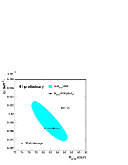
Figure 14: The Fermi coupling strength, $G_{F}$ versus the mass of the W boson as measured by the H1 collaboration [35].

Confronting the results from LEP, SLD and Tevatron, cast in the form of sin${}^{2}\theta_{w}$ in a $Q^{2}$ dependent extrapolation by Czarnecki and Marciano [36], with lower energy measurements we see in Fig. 14 good agreement with the atomic parity violation experiment on Cesium [38] and low energy Møller scattering from the E158 experiment [39]. For the NuTeV measurement [40] the situation has not changed since last year. It does not fit well with the expectation in the $Q^{2}$ range where the measurement has been made, being nearly three standard deviations off. It must be noted that in neutrino-nucleon scattering the $Q^{2}<0$, while in this figure it is compared to a determination at LEP at $Q^{2}>0$. The exact $Q^{2}$ in the NuTeV experiment varies event by event and this is accounted for by effectively fitting a running $\sin^{2}\theta$ to the data. The effect of the uncertainty on the average $Q^{2}$ scale is determined to be very small in [41].

4 The electroweak vector boson properties

The H1 collaboration delivered a first EW fit of their data, being able to extract the Fermi coupling strength and the mass of the W boson simultaneously [35], as shown in Fig. 14.

The W boson mass has been measured precisely at the second phase of LEP. The results for the W boson mass measurement are shown in Fig. 17. The OPAL experiment produced final results for this conference, while the ALEPH, DELPHI and L3 results are still preliminary.

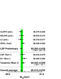
Figure 15: Summary and averages of measurements of $m_{\mathrm{W}}$.

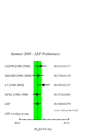
Figure 16: Measurements of $m_{\mathrm{W}}$ in the 4-jet final state.

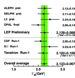
Figure 17: Measurements and average of $\Gamma_{\mathrm{W}}$.

The final OPAL measurement introduces a number of refinements, notably for the determination of possible systematic errors due to colour reconnection between the quarks from different W boson decays in WW$\rightarrow$4 jet events. The particle flow is studied between jets from the same and from different W’s in the event. A comparison for these intra- and inter-W particle flows is made to different models for and strengths of colour reconnection in Fig. 18. The comparison reveals no significant sign of colour reconnection and an upper limit of 37% of the strength predicted by the

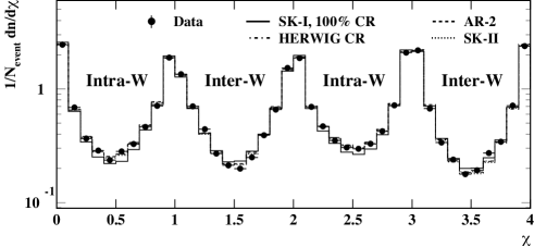
Figure 18: Measurement of the intra- and inter-W particle densities by the OPAL experiment [42]. The measurement is compared to several Monte Carlo models with and without colour reconnection.

Sjöstrand-Khoze-I model [43] is estimated at 95% CL. Soft particles are more susceptible to colour reconnection and Bose-Einstein correlation effects. OPAL reduced the colour reconnection uncertainty by cutting on particle momentum. The remaining uncertainty can be better estimated using the method of the intra- and inter-W particle flow measurement to be 49 MeV for colour reconnection and 22 MeV for Bose-Einstein correlations.

These two effects still remain the leading contributions to the overall systematic uncertainty on the $m_{\mathrm{W}}$ measurement. The current state for the $m_{\mathrm{W}}$ measurements from the WW$\rightarrow$4 jet channel is shown in Fig. 17. Similar reductions in error as for OPAL can be expected for the final results for $m_{\mathrm{W}}$ in this channel from the other LEP experiments.

The Tevatron experiments CDF and DØ had collected nearly 1 fb^-1 when this conference took place. Of that data volume typically about 300 pb^-1 has been analysed for final and preliminary results. Potentially, the CDF and DØ experiments will be able to measure the W boson mass with a precision similar to the LEP results. Crucial ingredient in this measurement is the Jet Energy Scale, which at present is not yet sufficiently under control to produce a competitive measurement.

The final OPAL results also lead to a new average $\Gamma_{\mathrm{W}}=2.123\pm 0.067$ GeV. Figure 17 shows the current state of the $\Gamma_{\mathrm{W}}$ measurements and average value.

At LEP-2 Z and W bosons can also be singly produced in a Zee and We$\nu$ final state respectively, which is well described by the SM as is shown in Fig. 19.

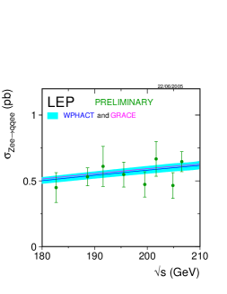
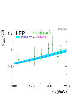
Figure 19: Cross section measurements for single Z (left) and W (right) boson production at LEP for energies between 180 and 210 GeV. Predictions based on WPHACT and Grace are also plotted.

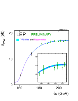
Figure 20: Cross section measurements for W-pair production at LEP and the predictions by the SM (YFSWW/RacoonWW).

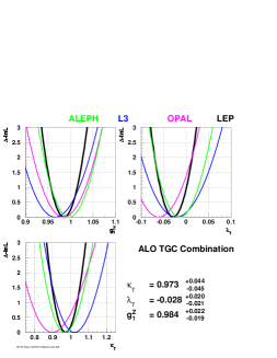
Figure 21: Fits for the W boson anomalous triple gauge boson couplings [44], based on W-pair production cross section and angular distributions as measured by ALEPH [45], L3 [46] and OPAL [47].

W-pair production in e⁺e^- scattering is sensitive to ZWW and $\gamma$WW triple gauge couplings. Another diagram contributing to W-pair production is neutrino exchange. Because of the structure of the SM, the couplings are in such a balance, that large cancellations occur in the cross section for e⁺e^-$\rightarrow$W⁺W^-, which prevents run-away of this cross section leading to violation of unitarity. This is nicely demonstrated in Fig. 21, where the measurement of all LEP experiments combined is compared to the SM, showing excellent agreement. In a slightly more sophisticated analysis the W-pair cross section and the angular distribution of the W’s can be used to derive the anomalous gauge couplings $\kappa_{\gamma}$, $\lambda_{\gamma}$ and $g_{1}^{\mathrm{Z}}$, which in the SM take the values 1, 0 and 1, respectively. Results of fits for these anomalous couplings are shown in Fig. 21. They are clearly in good agreement with the SM expectations. Triple gauge boson couplings also play an important role in the production of multiple gauge bosons in the same event at the Tevatron. Figure 23 shows the measurements of the cross sections for single and multi boson production for various combinations of bosons at the Tevatron. The SM predictions are superimposed and show good agreement with the measurements.

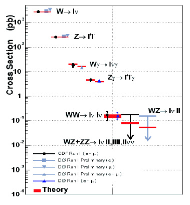
Figure 22: Cross sections for the production of multi boson final states at the Tevatron. The lines with an arrow downwards give measured upper limits for the cross section.

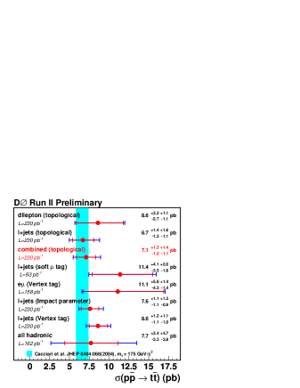
Figure 23: Summary of cross sections for the production of top pairs as measured at the Tevatron in different final state topologies.

5 Top quark properties

At the moment the Tevatron is the only accelerator that produces top quarks. Top quarks can be produced in pairs through the strong interaction and singly in weak processes. Top decays dominantly to a b-quark and a W boson, where the W decays again into hadrons or leptons. For $\mathrm{t}\overline{\mathrm{t}}$ events this leads to six experimental topologies: di-lepton events with a final state of $2\ell+2\mathrm{b}$+lots of missing transverse energy; lepton+jets events with a final state of $1\ell+4$ jets of which 2 jets are from b quarks and some missing transverse energy and; all-jets events which consist of six jets in the final state of which 2 are from b quarks.

The $\mathrm{t}\overline{\mathrm{t}}$ production cross section at the Tevatron is shown in Fig. 23. More details are given in the QCD contribution to these proceedings [3]. Single top production, important to measure the $V_{\mathrm{tb}}$ element of the Cabbibo-Kobayashi-Maskawa matrix (see [5, 6]), has not yet been observed by CDF and DØ at the Tevatron. Upper limits are given of 13.6 pb (CDF [48]) and 6.4 pb (DØ [49]) for $s$-channel production (W decay) and 10.1 pb (CDF [48]) and 5.0 pb (DØ [49]) for $t$-channel production (W exchange) all at 95% CL. This is in agreement with the SM model expectations of 0.88$\pm$0.07 pb and 1.98$\pm$0.21 pb for $s$- and $t$-channel respectively. The Tevatron limits are typically based on data corresponding to 200–250 pb^-1 of luminosity and a measurement may be expected in the next year or so.

An important property to measure is the top quark mass. The most important channel to do this is lepton+jets. The di-lepton channel has very small statistics, while the all jets channel suffers severe background. Event selection for the lepton+jets channel is done by identifying an electron or muon and four jets, followed by a topological selection and b-tagging. The signal to background ratio that can be observed is good, especially after b-tagging. The top mass is extracted by comparing observables to matrix elements and MC predictions, either via templates or another a priori probability density. The signal probability can be determined from theory by convoluting the cross section with a transfer function that models how the observables that the cross section depends on get smeared by fragmentation, detector resolution and analysis (such as jet finding method): CDF uses $m_{\mathrm{top}}$ directly as an observable, while DØ uses more elementary observables, such as lepton and jet energy and angles. These methods allow to simultaneously fit an overall Jet Energy Scale (JES) using the W-mass in the top-events to constrain it. This greatly reduces the uncertainty of the JES at the cost of a larger statistical error. The results of the analyses are listed in Fig. 25. Note the small systematic on the new results. The current preliminary top mass is $m_{\mathrm{top}}=172.7\pm 2.9$ GeV. Both experiments expect to go under an error of 2 GeV eventually in the Tevatron Run 2.

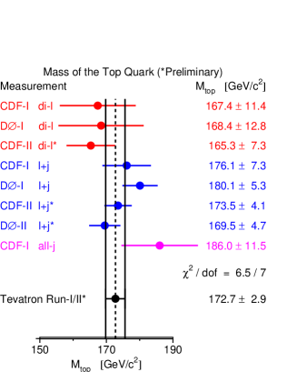
Figure 24: Measurements and average of the top quark mass.

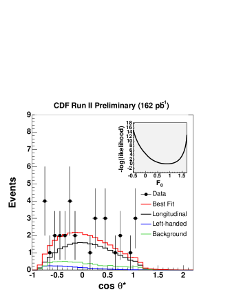
Figure 25: CDF measurement of the angle between the W and b quark in a top quark decay $\cos\theta^{*}\approx 2m_{\ell\mathrm{b}}^{2}/\!\!\!\left(m_{\mathrm{top}}^{2}-m_{\mathrm{W}}^{2}\right)-1$.

As pointed out by Grünewald [50] there might be a systematic trend in the top quark mass determinations depending on the decay topology, which may become important as the determination becomes more accurate.

Because the top quark decays before it hadronises, its helicity can be measured through the angular distribution of its decay products. The angle between the W and the b quark from the top decay in the top rest frame can be approximated as $\cos\theta^{*}\approx 2m_{\ell\mathrm{b}}^{2}/\!\!\!\left(m_{\mathrm{top}}^{2}-m_{\mathrm{W}}^{2}\right)-1$. In Fig. 25 the distribution of this angle $\cos\theta^{*}$ is plotted as measured by the CDF collaboration. The $\cos\theta^{*}$ distribution is fitted to three helicity components: $f_{0}$ with W direction along the top spin, W spin transverse to the top spin and b quark spin along the top spin; $f_{-}$ with W direction opposite the top spin, W spin along the top spin and b quark spin opposite to the top spin; and $f_{+}$ with W direction along the top spin, W spin along the top spin and b quark spin opposite to the top spin. The SM expectations for these quantities are $f_{0}\approx 0.7$, $f_{-}\approx 0.3$ and (due to the purely $V-A$ coupling) W $f_{+}=0$. Also other angular information can be used in a similar way, such as the transverse moment of the lepton from the W decay and the invariant mass of the lepton from the W decay and the b quark from the top decay. From the fit to the $\cos\theta^{*}$ distribution CDF determined $f_{0}=0.89_{-0.34}^{+0.30}\pm 0.17$ [51]. Another CDF measurement uses a combination of di-lepton channel and the lepton+jets channel of t$\overline{\mathrm{t}}$ events to obtain $f_{0}=0.27_{-0.21}^{+0.35}$ [52]. lepton+jets channel of t$\overline{\mathrm{t}}$ events. and $f_{+}<0.18$ at 95% CL [53], whereas DØ determined that $f_{+}=0.04\pm 0.11\pm 0.06$ in the combination of the di-lepton and lepton plus jets channels [54]. These results are all fully compatible to the SM prediction.

Using the fact that in $\mathrm{t}\overline{\mathrm{t}}$ events there is a b quarks from both tops in the final state and by counting the number of zero, one or two b-tagged jets, the ratio of top quarks decaying into a b quark over any top decay, $R=\mathrm{B}(\mathrm{t}\rightarrow\mathrm{Wb})/\mathrm{B}(\mathrm{t}\rightarrow\mathrm{Wq})\approx|V_{\mathrm{tb}}|^{2}$, can be measured and thus $|V_{\mathrm{tb}}|$. The results give rise to the limits $|V_{\mathrm{tb}}|>0.78$ by CDF [55] and $|V_{\mathrm{tb}}|>0.80$ by DØ [56] both at the 95% CL, well compatible with $|V_{\mathrm{tb}}|\approx 1$.

6 The EW fit and prediction of the SM Higgs mass

$\Delta\alpha_{\mathrm{had}}$ =	0.02767	$\pm$ 0.00034
$\alpha_{\mathrm{s}}$ =	0.1186	$\pm$ 0.0026
$m_{\mathrm{Z}}$ =	91.1874	$\pm$ 0.0021	GeV
$m_{\mathrm{top}}$ =	173.3	$\pm$ 2.7	GeV
$m_{\mathrm{H}}$ =	91	${}_{-32}^{+45}$	GeV

Correlation
coefficients	$\Delta\alpha_{\mathrm{had}}$	$\alpha_{\mathrm{s}}$	$m_{\mathrm{Z}}$	$m_{\mathrm{top}}$
$\alpha_{\mathrm{s}}$	0.01
$m_{\mathrm{Z}}$	-0.01	-0.02
$m_{\mathrm{top}}$	-0.02	0.05	-0.03
$\log(m_{\mathrm{H}}/(1~{}\mathrm{GeV})$	-0.51	0.11	0.07	0.52

Table 1: Results of the electroweak fit as performed by the LEP EW Working Group [50].

Fitting all relevant LEP, SLD and Tevatron electroweak measurements simultaneously as is done by the LEP ElectroWeak Working Group yields, when using also the $\Delta\alpha_{had}$ from Burkhardt and Pietrzyk, the outputs shown in Fig. 12. and Table 1 The only SM parameter without direct experimental determination is the SM Higgs boson mass, $m_{\mathrm{H}}$. The fit gives an indirect determination of log$(m_{\mathrm{H}})=1.96\pm 0.18$. The fit has a $\chi^{2}/$d.o.f.$=17.8/13$ corresponding to a fit probability of 16.5%. Looking at the correlation matrix between the fit parameters also given in Table 1, it becomes clear why above relatively much attention was given to $\Delta\alpha_{had}$ and $m_{t}$ in view of the importance to determine $m_{\mathrm{H}}$.

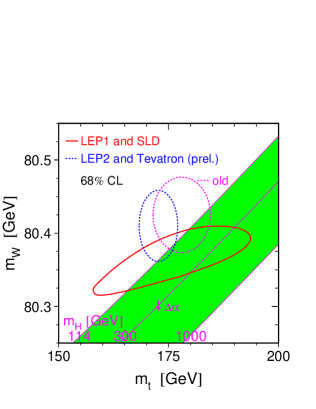
Figure 26: Probability contours (ellipses) at 68% CL of the EW fit in the $m_{\mathrm{top}}$–$m_{\mathrm{W}}$ plane. The ellipse indicated as “old” is the one that was presented at the Lepton-Photon conference in summer 2005. The grey area is the SM prediction for various Higgs boson masses, that label de diagonals.

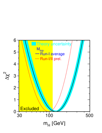
Figure 27: Difference in $\chi^{2}$ with respect to the best fit, as a function of the Higgs boson mass. The dotted curve is the current preliminary fit for which the theoretical error has not yet been established. The band is an older fit and can be used as an indicator for the theoretical uncertainty. In light grey the Higgs boson mass range that has been excluded by direct searches at LEP.

Comparing $m_{\mathrm{}W}$ and $m_{\mathrm{top}}$ from direct and indirect measurements to the SM expectation in Fig. 27, a consistent picture arises with a preference for a low Higgs mass. Compared to last year, notably the $m_{t}$ measurement improved considerably, but the qualitative conclusion has hardly changed. In Fig. 27 the situation for the prediction of the Higgs boson mass is summarised. When the probability from the $\chi^{2}$ values is normalised to only include the Higgs mass range above the direct search limit (see next section) as possibilities, an upper limit for the SM Higgs boson mass can be derived of $m_{\mathrm{H}}<219$ GeV at 95% CL.

7 Direct search for the SM Higgs

At LEP-2 the Higgs boson has been primarily searched for in the production channel in which it is radiated off a virtual Z boson. The fact that no clear signal for Higgs boson production has been observed at LEP-2 has lead to a lower limit of the possible mass of the Higgs boson of $m_{\mathrm{H}}>114.4$ GeV at 95% CL by combining the searches in all possible final state channels by all LEP experiments [57]. Although this limit is still preliminary, it is quite stable for a while now.

The current best place to look for a Higgs boson in the mass range from 114 to 219 GeV is at the Tevatron. In Fig. 29 and 29 the cross section for SM Higgs production in the main channels and the branching ratios for the decay of the SM Higgs boson are plotted.

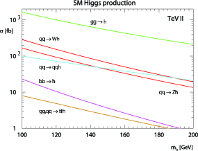
Figure 28: Cross section for SM Higgs production at the Tevatron at $\sqrt{(}s)=1.96$ TeV as a function of the Higgs mass in the various production channels.

Figure 29: Branching ratio of the SM Higgs boson as a function of their mass in the various decay channels.

H decay is up to $m_{\mathrm{H}}=135$ GeV dominantly into b$\overline{\mathrm{b}}$ and above that into WW^(∗) (where one of the W’s is often off-shell). Most of the region of interest is in the overlap region where both decays have a non-negligible branching fraction. H$\rightarrow$b$\overline{\mathrm{b}}$ has large backgrounds and is easiest searched for when the Higgs is produced in association with a W or Z that decays leptonically, giving a charged lepton and/or missing $E_{\mathrm{T}}$ trigger. Lifetime or

soft lepton b quark tagging is used to identify the jets from H decay. The background mostly consists of W or Z plus jets and is getting progressively better understood from the data and Monte Carlo. The expected signal to background ratio is not very large. H$\rightarrow$WW^(∗) can be selected in the channel where one or both W’s decay leptonically to electron or muon. A promising channel is WH production followed by H$\rightarrow$WW^(∗), where of the 3W’s produced the like-sign pair is selected through leptonic decay, allowing a very clean selection.

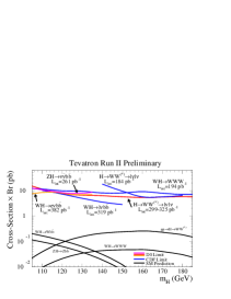
Figure 30: Cross section times branching ratio upper limits at 95% CL for Higgs production at the Tevatron at $\sqrt{(}s)=1.96$ TeV as a function of the Higgs mass in the various search channels as indicated for the curves in the upper part of the figure [58]. In the lower part of the figure the SM cross section times branching ratio are given for the relevant production and decay topologies.

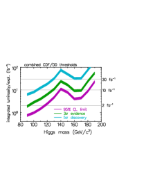
Figure 31: Summary of exclusion or discovery range as a function of the Higgs mass for the Tevatron Run 2, as reported by the Tevatron Higgs Working Group in 2000 [59]. The lower band indicates the average luminosity for which a 95% CL limit on the existence of the Higgs can be obtained as a function of the Higgs mass. The middle and upper curve show the average luminosity at which a three or five standard deviation discovery can be made as a function of the Higgs mass.

Combining all current, mostly preliminary results, the picture arises as shown in Fig. 31. It is clear from this figure that the present sensitivity is at least an order of magnitude away from being able to exclude the existence of the Higgs boson at mass ranges above the values excluded by the direct searches at LEP. In 1999 and 2000 a study was made of the Tevatron Run 2 sensitivity to exclude or discover the Higgs. The predicted result is shown in Fig. 31. Comparing the current cross section limit results in Fig. 31 to the Working Group expectations, the H$\rightarrow$b$\overline{\mathrm{b}}$ part is currently nearly a factor of 10 under the expected sensitivity. However improvements by a factor 4 in b-tagging and another factor of $\sqrt{2}$ by using both the electron and muon decay channels of the W can be attained. Another factor of up to $\sqrt{2}$ can be reached by considering a larger range in geometric acceptance than only the central region presently considered. These are the first generation of results for these searches and additional gain in sensitivity by refining the search strategy can be expected. All in all the projected sensitivity from the Working Group back in 2000 seems attainable.

In the H$\rightarrow$WW^(∗) regime we are still a factor of 2 under the expected sensitivity. But also here improvements are worked on, although a single improvement that gives a large part of this factor cannot easily be identified and the gain is likely to come from a number of small improvements.

There was an update of the sensitivity prediction in 2003, showing a larger sensitivity [60]. Attaining this sensitivity seems only possible in an optimistic scenario.

8 Prospects for Higgs discovery in the next few years

A striking feature in Fig. 31 is the middle of this plot which is shared by all three curves. This bump is in the overlap regime between the Higgs dominantly decaying to b$\overline{b}$ or WW^(∗). However, in the figure describing the actual measurement, Fig. 31, the cross section limit has a smooth behaviour, even after the improvements mentioned before. Also the SM cross section times branching ratio limits shown in this same figure are approximately flat over the whole relevant Higgs mass range. It is therefore reasonable to assume that the bump in the prediction of Fig. 31 will in reality not occur. Assuming that in the pure H$\rightarrow$b$\overline{\mathrm{b}}$ and H$\rightarrow$WW^(∗) the sensitivity indicated in Fig. 31 will be attained and the results are carefully combined in the intermediate overlap region, the prediction for the sensitivity becomes that of Fig. 33.

Figure 32: Prospects for the baseline and design integrated luminosity per experiment for the Tevatron [61]. The insert shows in more detail the integrated luminosity prospects and achievements up to the date of the conference.

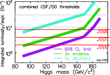
Figure 33: Version revised by the author of the exclusion or discovery range as a function of the Higgs mass for the Tevatron Run 2. The coding of the bands is as in Fig. 31. On the right hand side the year is indicated when a certain integrated luminosity is taken as predicted in Fig. 33.

In this figure the luminosity levels are indicated that should be attained according to the Tevatron design luminosity projections at the end of 2006 (2 pb${}^{-}1$), the end of 2007 (5 pb${}^{-}1$) and by the summer of 2009 (8 pb${}^{-}1$), according to the predictions in Fig. 33. It should be noted that thus far the Tevatron has delivered a luminosity equal to or exceeding the design values and several upgrades to the Tevatron are planned to maintain this trend.

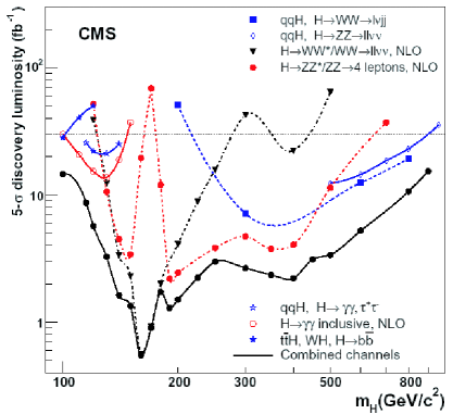
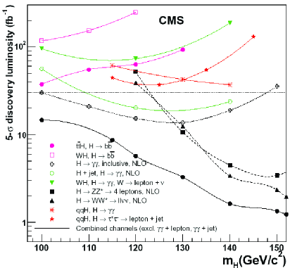
Figure 34: Prediction for the luminosity needed to discover the SM Higgs boson with the CMS detector at the LHC as a function of the Higgs mass [62].

Clearly the next stop after the Tevatron to discover the Higgs boson and measure its properties is the LHC. In Fig. 34 the discovery potential for the SM Higgs boson is given for the CMS experiment. The ATLAS experiment has very similar sensitivity. In this figure the approximate integrated luminosities that correspond with one and two years of running are also indicated. If the LHC turns on as scheduled in 2007 and serious luminosity acquisition is taken starting early 2008, discovering the SM Higgs will be a photo-finish between the LHC and the Tevatron. Taking the end of 2007 as a benchmark, the Tevatron may have excluded the SM Higgs up to 160 GeV. This is excellent news for the LHC: the SM Higgs is right where the LHC experiments are most sensitive, where the Higgs branching ratio to W- and Z-pairs is large. Alternatively, a hint of a Higgs with mass below 120 GeV may be present: Again good news for the LHC: the SM will break down in the TeV range, and the LHC will probably find signals of physics beyond the SM.

9 Summary and conclusion

The electroweak sector of the SM is in excellent overall agreement with the available body of measurements. The parts that are least in accordance with the SM predictions are the lepton asymmetry from SLD measurements and the effective $\sin^{2}\theta_{w}$ measurement from NuTeV. Improvement in the determination of the hadronic correction to $\alpha_{\mathrm{QED}}$ is needed to resolve possible discrepancies to describe the muon anomalous magnetic moment. Improvements in $\alpha_{\mathrm{QED}}(M_{\mathrm{Z}})$, $m_{\mathrm{W}}$ and $m_{\mathrm{top}}$ will lead to a better estimate of the Higgs boson mass, the only particle from the SM that has not yet been observed. The precision of the measurements and SM predictions allow a mass range $114<m_{\mathrm{H}}<219$ GeV at better than 95% Confidence Level. A Standard Model Higgs in this mass range will likely be observed in the years 2007–2010, either at the Tevatron or at the LHC.

References

- [1] S. Weinberg, Phys. Rev. Lett. 19 (1967) 1264; A. Salam, p. 367 of Elementary Particle Theory , ed. N. Svartholm (Almquist and Wiksells, Stockholm, 1969); S.L. Glashow, J. Iliopoulos, and L. Maiani, Phys. Rev. D2 (1970) 1285; G. ’t Hooft, Nucl. Phys. B35 (1971) 167.
- [2] M. Gell-Mann, Phys. Letters 8, 214 (1964); G. Zweig, CERN Reports No. 8182/TH. 401 and No. 8419/TH. 412, 1964 (unpublished); Bjorken and Feynman 1968-1969. R.P. Feynman, Proceedings of the Third high Energy Conference at Stony Brook (Gordon and Breach, 1970); J.D. Bjorken, Proceedings of the 1967 International School of Physics at Varenna (Academic Press, 1968).
- [3] T. Greenshaw, these proceedings.
- [4] C. Davies, these proceedings.
- [5] G.C. Branco, these proceedings.
- [6] M.H. Shune, these proceedings.
- [7] J. Klein, these proceedings.
- [8] F. Sanchez, these proceedings.
- [9] For a written out version of the SM Lagrangian see e.g. Martinus Veltman, Diagrammatica, the Path to Feynman Diagrams, Cambridge University Press, 1994, Appendix E.
- [10] J. Erler and P. Langacker in: S. Eidelman et al., Phys. Lett. B592 (2004) 1, http://pdg.lbl.gov.
- [11] L3 Collaboration, P. Achard et al., Phys. Lett. B616 (2005) 145.
- [12] OPAL collaboration, G. Abbiendi et al., [hep-ex/0505072]
- [13] L3 Collaboration, M. Acciarri et al., Phys. Lett. B476 (2000) 40.
- [14] S. Mele, these proceedings.
- [15] A. Höcker, in proceedings of ICHEP04, Vol. 2 pp. 710-715, [hep-ph/0410081].
- [16] F. Jegerlehner, Nucl. Phys. Proc. Suppl. 126 (2004) 325.
- [17] V.V. Ezhela, S.B. Lugovsky, O.V Zenin, [hep-ph/0312114].
- [18] K. Hagiwara, A.D. Martin, D. Nomura, T. Teubner, Phys. Rev. D69 (2004) 093003.
- [19] J.F. de Troconiz, F.J. Yndurain Phys. Rev. D71 (2005) 073008.
- [20] M. Davier, S. Eidelman, A. Hocker, Z. Zhang, Eur. Phys. J. C31 (2003) 503.
- [21] Muon Collaboration, G.W. Bennett et al., Phys. Rev. Lett. 92 (2004) 161802.
- [22] M. Passera, these proceedings and J. Phys. G31 (2005) R75.
- [23] L3 Collaboration, M. Acciarri et al., Phys. Lett. B623 (2005) 26.
- [24] P.J. Mohr and B.N. Taylor, Rev. Mod. Phys. 72 (2000) 351.
- [25] N. Cabbibo, R. Gatto, Phys. Rev. 124 (1961) 1577.
- [26] H. Burkhardt, B. Pietrzyk, Phys. Rev. D72 (2005) 057501.
- [27] ALEPH Collaboration, S. Schael et al., Phys. Rep. 421 (2005) 191.
- [28] D. Leone for the KLOE Collaboration, these proceedings.
- [29] I. Logashenko on behalf of the CMD-2 Collaboration, these proceedings.
- [30] S. Serednyakov for the SND Collaboration, these proceedings and [hep-ex/050676].
- [31] H. Hayashii for the Belle Collaboration, these proceedings.
- [32] H. Kaji on behalf of the H1 and ZEUS Collaborations, these proceedings.
- [33] The LEP Collaborations, the ALEPH Collaboration, the DELPHI Collaboration, the L3 Collaboration, the OPAL Collaboration, the LEP Electroweak Working Group, the SLD electroweak, heavy flavour groups, Precision Electroweak Measurements on the Z Resonance, [hep-ex/0509008], Submitted to Phys. Rep.
- [34] CDF Collaboration, Phys. Rev. D71(2005) 052002.
- [35] H1 Collaboration, Determination of Electroweak Parameters at HERA, [hep-ex/0507080], Submitted to Phys. Lett. B.
- [36] A. Czarnecki and W.J. Marciano, Int. J. Mod. Phys. A15 (2000) 2365.
- [37] Particle Data Group, S. Eidelman et al., Phys. Lett. B592 (2004) 1, http://pdg.lbl.gov.
-
[38]
C.S. Wood et al.,
Science 275 (1997) 1759;
S.C. Bennett and C.E. Wieman, Phys. Rev. Lett. 82 (1999) 2484. - [39] SLAC E158 Collaboration, P.L. Anthony et al., Phys. Rev. Lett. 95 (2005) 081601
- [40] NuTeV Collaboration, G.P. Zeller et al., Phys. Rev. Lett. 88 (2002) 091802, Erratum-ibid.90 (2003) 239902; NuTeV Collaboration, G.P. Zeller et al., Phys. Rev. D65 (2002) 111103, Erratum-ibid. D67 (2003) 119902; NuTeV Collaboration, G.P. Zeller et al., Reply to the Comment on “A Precise Determination of Electroweak Parameters in Neutrino-Nucleon Scattering”, [hep-ex/0207052].
- [41] G.P. Zeller, A Precise Measurement of the Weak Mixing Angle in Neutrino-Nucleon Scattering, PhD thesis at Northwestern University, June 2002, FERMILAB-THESIS-2002-34.
- [42] The OPAL Collaboration, G. Abbiendi et al., Colour reconnection in e+e-W+W- at GeV, [hep-ex/0508062], Submitted to Eur. Phys. J. C.
- [43] T. Sjöstrand and V.A. Khoze Z. Phys. C62 (1994) 281.
- [44] The LEP Collaborations ALEPH, DELPHI, L3 and OPAL and the LEP TGC Working Group, A Combination of Results on Charged Triple Gauge Boson Couplings Measured by the LEP Experiments, LEPEWWG/TGC/2005-01, June 8, 2005.
- [45] ALEPH Collaboration, Phys. Lett. B614 (2005) 7.
- [46] L3 Collaboration, Phys. Lett. B586 (2004) 151.
- [47] OPAL Collaboration, Eur. Phys. J. C33 (2004) 463.
- [48] CDF Collaboration, D. Acosta et al., Phys. Rev. D71 (2005) 012005.
- [49] Search for single top quark production in p anti-p collisions at TeV, DØ Collaboration, V.M. Abazov et al., Phys. Lett. B622 (2005) 265.
- [50] M. Grünewald, these proceedings.
- [51] CDF Collaboration, Measurement of W boson Polarization in Top Quark Decays using at CDF II, CDF/ANAL/TOP/PUB/7173, August 12, 2004.
- [52] CDF Collaboration, Measurement of the Fraction of Longitudinally-Polarized W bosons Produced in Top-Quark Decays in 200 pb-1 of Collisions at TeV, CDF note 7058, July 6, 2004.
- [53] CDF Collaboration, D. Acoste et al., Measurement of the W boson Polarization in Top Decay at CDF at TeV, APS/123-TOP, 19th November 2004. July 6, 2004.
- [54] DØ Collaboration, Combination of b-tagged and Topological Measurement of the W Helicity in Top Quark Decays, DØnote 4839-CONF, July 6, 2005.
- [55] CDF Collaboration, D. Acoste et al., Phys. Rev. Lett. 95 (2005) 102002.
- [56] DØ Collaboration, Simultaneous measurement of B(tWb)/B(tWq) and at DØ, DØnote 4833-CONF, June 15, 2005.
- [57] LEP Working Group for Higgs boson searches and ALEPH Collaboration and DELPHI Collaboration and L3 Collaboration and OPAL Collaboration, R. Barate et al., Phys. Lett .B565 (2003) 61.
-
[58]
The CDF Collaboration,
Search for New Particles
Production in Association with Bosons in
Collisions at TeV,
CDF/PUB/EXOTIC/PUBLIC/7740, July 5, 2005;
The CDF Collaboration,
Search for a Standard-Model Higgs Boson
in WW Dilepton Decay
Channels with 200/pb Run II Data at CDF,
http://www-cdf.fnal.gov/physics/exotic/run2/higgs-ww-2004/index.htm;
The CDF Collaboration,
Search for the WH Production Using High- Isolated Like-Sign
Dilepton Events in Run II,
CDF/PUB/EXOTIC/PUBLIC/7307, October 24, 2004;
The DØ Collaboration, Search for the Higgs boson in HWW(∗) () decays in collisions at TeV, DØnote 4760-CONF, March 14, 2005; DØ Collaboration, V.M. Abazov et al., A Search for Wb and WH Production in p Collisions at TeV, Fermilab-Pub-04/288-E, February 1, 2005; The DØ Collaboration, A Search for SM Higgs boson using the channel in Collisions at TeV, DØnote 4774-CONF, April 14, 2005. - [59] M. Carena et al., Report of the Tevatron Higgs Working Group, [hep-ph/0010338].
- [60] CDF and DØ Collaborations, Results of the Tevatron Higgs Sensitivity Study, Preprint FERMILAB-PUB-03/320-E, October 17, 2003.
- [61] The defintions of the baseline and design luminosity for the Tevatron are given in: The Run II Luminosity Upgrade at the Fermilab Tevatron, Project Plan and Resource-Loaded Schedule, plan submitted by FNAL to DoE, June 15, 2003, http://www-bd.fnal.gov/doereview03/docs/Overview7.1.pdf.
- [62] Jorgen D′Hondt on behalf of the CMS Collaboration, these proceedings.